capacity of vehicular ad hoc networks based on multibeam

Research ArticleCapacity of Vehicular Ad Hoc Networks Based on MultibeamDirectional Transmission

Yuhua Wang , Laixian Peng , and Renhui Xu

Army Engineering University of PLA, Nanjing 210000, China

Correspondence should be addressed to Laixian Peng; [email protected]

Received 9 August 2021; Revised 30 September 2021; Accepted 9 October 2021; Published 26 October 2021

Academic Editor: Renchao Xie

Copyright © 2021 Yuhua Wang et al. This is an open access article distributed under the Creative Commons Attribution License,which permits unrestricted use, distribution, and reproduction in any medium, provided the original work is properly cited.

The development of multibeam directional transmission technology used in vehicular ad hoc networks is drawing much moreattention in recent years due to its wider coverage ability than omnidirectional transmission. In this paper, we analyse thetransport capacity of the vehicular network using different antenna modes in the transmitter and receiver end, respectively. Wefirst construct the cross-layer model comprising the characteristic of the directional antenna model, arbitrary network model,and interference model. Then, based on scaling laws, we calculate the upper and lower bound of the network capacity with andwithout the directional multibeam transmission technology. In order to reduce the capacity lower bound computationcomplexity, several topology frameworks are constructed while taking various interferences into account included in the actualproject. Finally, we analyse the capacity under changes of different parameters and also evaluate the law of capacity changes todiscover how much improvement multibeam transmission technology can bring to the network performance. Analysis showsthat compared with DTOR and OTDR mode, DTDR mode can continue to increase network capacity by 2 to 3 times on thebasis of the above two modes.

1. Introduction

Network capacity is one of the most important indicators toevaluate vehicular ad hoc network (VANET) communica-tion performance. It can provide theoretical support for thetechnical development of wireless network communicationand transmission. Given any set of successful transmissionstaking place over time and space, let us say that the networktransports one bit-meter when one bit has been transporteda distance of one meter toward its destination. Summing allproducts of bits and the distances over which they are car-ried is a valuable indicator of a network’s transport capacity.Nodes in the VANET are often mobile, and their communi-cation links have time-varying characteristics; therefore, itsnetwork topology is unstable. Due to the nature of wirelesstransmission, the capacity of a wireless network is strictlylimited by the number of nodes per unit area and the chan-nel transmission bandwidth. Since Gupta and Kumar [1]proposed the investigating method of network capacity inwireless ad hoc networks based on omnidirectional trans-mission, many researches have focused on this field. They

proposed that the network capacity is ΘðW ffiffiffin

p Þ under thearbitrary network model, where n nodes are arbitrarilyplaced in a disk of unit area and the channel bandwidth isW. Knuth notation is used to express this result, where f ðnÞ =Θ½gðnÞ� means f ðnÞ and gðnÞ have the same growthlevel.

According to these researches, many calculations for theupper and lower bounds of wireless ad hoc network capacityand methods to improve network transmission capacity andthroughput capacity have been proposed. However, theomnidirectional transmission mode has several disadvan-tages such as it owns a large attenuation level, inefficientuse of transmit power, and all nodes near a pair of commu-nication nodes need to remain silent in order to transmitsuccessfully and so on. In order to significantly improvethe spatial multiplexing of wireless channels, thereby thecapacity and throughput, directional antenna transmissiontechnology was proposed. When using directional antennas,multiple pairs of nodes located near each other can transmitat the same time without mutual interference, which onlydepends on the directional characteristic of the directional

HindawiWireless Communications and Mobile ComputingVolume 2021, Article ID 1036689, 18 pageshttps://doi.org/10.1155/2021/1036689

https://orcid.org/0000-0002-8691-6233

https://orcid.org/0000-0002-6580-1349

https://creativecommons.org/licenses/by/4.0/

https://doi.org/10.1155/2021/1036689

antenna. The emergence of the adaptive multibeam arrayantenna transmission technology makes each node commu-nicate with other nodes in multiple directions at the sametime, which further improves the network communicationcapability.

A method of network capacity calculation when usingdirectional transmission technology in wireless ad hoc net-works was proposed in [2]; it came out that the antenna modelwas simplified to a sector-shaped antennamodel that only con-sidered the main lobe effect and ignored the side lobe effect. Inthis model, the directional working beam sector area was com-pared with the entire circular radiation range. The research in[3] was continued on the basis of [2]; it deduced the upperand lower bounds of network capacity in the case of single-hop and multihop communication. It indicated that the capac-ity increases as the number of hops increases when in a certainrange and becomes smaller when the number of hops exceedsthis range. In [4], a hybrid antenna model used in single-beam mode was proposed. This model considers the influenceof the side lobe effect on the network capacity when actual sit-uations are taken into account and simplifies the effect as a cal-culation factor that could be inserted into the derivationprocess. Similarly, in [5], they put forward that the influenceon capacity caused by multibeam could be converted into again factor which could be easily used in the derivation processas well. A more convergent lower bound of the capacity calcu-lating method under arbitrary network model was put forwardin [6]. In [7], the influence of self-interference caused by beam-forming on network capacity is studied, which lead us to thinkabout the difference between the side lobe effect and self-interference. Different from the multibeam technology, Rah-man et.al in [8] discussed from the perspective of multipacketreception to explore what kind of improvement their protocolwill bring to network performance. In [9, 10], theymainly stud-ied the improvement of network performance by cross-layerprotocols and explored optimization strategies.

What is more, besides the discussion of the networkcapacity according to the node deployment method (thatis, the protocol model in [1]), the analyses at the physicallayer are also diverse. The research in [11] started with thepower allocation in the physical layer, considered differentpower allocation modes for different transmission links,and analysed the optimal value of the network capacityunder this condition. In [12], Zhao et al. considered thecapacity of cellular network. From the perspective of anothernetwork model, the results could be mutually confirmedwith the conclusion in [1]. The latest research achievementsare focused on a more comprehensive theoretical model. In[13], a way was proposed to expand network capacitythrough MIMO technology when smart antennas are used;this is much like the multibeam technology to be analysedin our research. In [14], the use of millimeter wave multi-beam transmission mode in the satellite layer network wasconsidered to increase the overall network capacity, whichcan be mutually confirmed with the VANET capacity calcu-lated by us. In [15–18], their researches are aimed at improv-ing the performance of the network through the algorithm ofresource scheduling and obtaining the maximum networkcapacity by assigning different bandwidths to different

nodes. Research on the control of output power mode inorder to pursue a more optimal network capacity is reflectedin [19–22]; different nodes choose different transmit powersaccording to different task requirements, which can effec-tively improve the throughput of the topology.

When it comes to the analysis of the capacity in vehicu-lar ad hoc networks, several researches have focused theirefforts on this zone. In [19, 23–25], they investigate architec-ture and applications of the VANET in order to look for arelatively comprehensive vehicle connectivity agreement toensure users’ security.

However, when calculating the arbitrary network capac-ity, few predecessors have done the overall derivation of themultibeam technology; they just analyse single-beam modecomprehensively. In their researches, the analyses on theimprovement of network capacity brought by directionaltransmission technology and multibeam technology are stillin a very ideal state, and there are still many details that havenot been considered in actual engineering applications.

Therefore, this paper mainly studies the network capacityof the VANET and analyses how much improvement the net-work capacity can be brought to by the use of multibeamdirectional transmission technology compared with the tradi-tional antenna working mode. When computing the capacity,we fully take the influence of the directional antenna side lobeeffect on the network capacity into account and derive theupper and lower bound of the arbitrary network capacitywhen the transceiver node pairs use the following four work-ing modes. These working modes are omnidirectional trans-mission and omnidirectional reception, omnidirectionaltransmission and directional reception, directional transmis-sion and omnidirectional reception, and directional transmis-sion and directional reception. They will be abbreviated asOTOR, OTDR, DTOR, and DTDR in the rest of this paper.Finally, under normalized conditions, we compared theimprovement of network capacity in several modes and foundout the conditions that need to be satisfied in this case.

Our main contribution can be summarized as follows:

(1) We conduct a more in-depth study on the networkcapacity using directional multibeam technologyand take the side lobe effect into account on the anal-ysis of the wireless network capacity at the sametime, which would make the results to have morerealistic significance. Capacity analyses on differenttransmission model have been carried out as well

(2) We horizontally compare the convergence of the net-work capacity under different interference models andexplore how to select the interference model if theupper and lower bounds of the wireless networkcapacity are sensitive to the various model parameters

(3) We longitudinally compare the changes in networkcapacity performance under different antenna modesand find the conditions which make the networkcapacity be maximized

The rest of the paper is organized as follows. In Section2, we will describe the models we built and parameters we

2 Wireless Communications and Mobile Computing

should use, and then, we will explain their meanings. In Sec-tions 3 and 4, we will discuss the upper and lower bounds ofthe arbitrary network model under two interference models(the protocol model and the physical model). In Section 5,we analyse the results obtained in the previous two sections.In Section 6, we will summarize and analyse our results andthen describe future research directions.

2. Parameters and Models

In this section, meanings of all symbols and parameters usedin the following derivation process will be explained andlisted in Table 1. At the same time, in order to make the sub-sequent derivation concise, we make some reasonableassumptions to obtain a more convenient calculation pro-cess and they are as follows:

(1) There are n vehicular nodes arbitrarily located in adisk of unit area on the plane. (The results carry overto any domain of unit area in R2 which is the closureof its interior.) Each node can transmit W bits persecond over a common wireless channel

(2) All nodes transmit with the same transmitting powerP, which would make the calculation process lesscomplex

(3) The transmitting or receiving beam width in themultibeam transmission model is identical, that is,all nodes share the same kind of adaptive multibeamarray antenna and the same antenna state

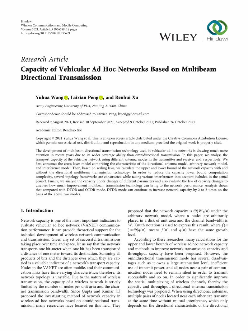
2.1. Antenna Model. Most of the existing studies on thecapacity of directional transmission networks use the simpli-fied sector-based directional antenna model. This model cansimplify the calculation process, but it ignores the influenceof the side lobe effect on the calculation results, which makesresults somewhat idealized. The hybrid antenna model is ref-erenced in [4]. This model takes the side lobe effect and theantenna directional characteristic into account and handlesthe complexity of the calculation process well. In ourresearch, the multibeam directional transmission modeneeds to change the directional sector range (the numberof beams) in it. The model is shown in Figure 1.

The model in the figure is a hybrid model of omnidirec-tional and directional modes. The sector area with a largerradius than the circular area represents the main lobe direc-tion, whose beam angle is θ, and the remaining circular areais surrounded by side lobes and back lobes, where the radiusof the circle and the sector represents the length of the omni-directional and directional radiation, respectively. We definethe parameter s as the ratio of the radius of Gside and Gmain inthe hybrid antenna mode, which is generally less than 1. Thegain of the omnidirectional antenna is Gside as well. It can beseen that nodes can simultaneously receive signals fromtransmitters in the circular area and the sector area.

2.2. Network Model. We use the arbitrary network model inthe following derivation process. In the setting of arbitrarynetwork model, there are n nodes arbitrarily located in a

region of unit area (e.g., 1m2). Each node arbitrarily selectsa target node for to communicate, and it sends data to thetarget node at an arbitrary transmission rate. Therefore,the data transmission flow is random, and these nodes canarbitrarily choose the transmission distance and power level.

2.3. Interference Model. In a wireless ad hoc network, ifnodes are densely distributed to a certain extent, concurrenttransmission will occur, which will cause mutual interfer-ence. Therefore, nodes need to be deployed separately toavoid conflicts in the cross area. For this reason, we assumethat there are interference areas that can guarantee success-ful transmission. Relying on the protocol model and physicalmodel proposed by Gupta et al. in [1] and the interferencearea theory of directional transmission proposed by Yiet al. [2], we made a certain degree of improvement on thisbasis to establish an interference area model based on thereceived signal.

2.3.1. Protocol Model. Suppose node Xi transmits to a nodeXj. Then, in order for this transmission to be successfulwhen node Xk simultaneously transmits over the same chan-nel, this condition needs to be satisfied.

Xk − Xj

�� ≥ 1 + Δð Þ Xi − Xj

�� , ð1Þ

where Xi, Xj, Xk, and Xl refer to the nodes themselves andtheir current positions. The constant Δ > 0 models situationswhere a guard zone is specified by the protocol to prevent aneighboring node from transmitting at the same time. It alsoallows for imprecision in the achieved range of transmissions.

2.3.2. Physical Model. On the premise that the receiver SINRthreshold β (minimum SINR) is specified, the condition forthe node Xj to successfully receive the data transmitted fromthe node Xi is

SINR =PC GtGr/ Xi − Xj

�� α� �N +∑ k∈Γ

k≠iPC ·GtGr/ Xk − Xj

�� α� � ≥ β, ð2Þ

where Gt means the gain of transmitting antennas and Grmeans the gain of receiving antennas. In most cases, β ≥ 1.

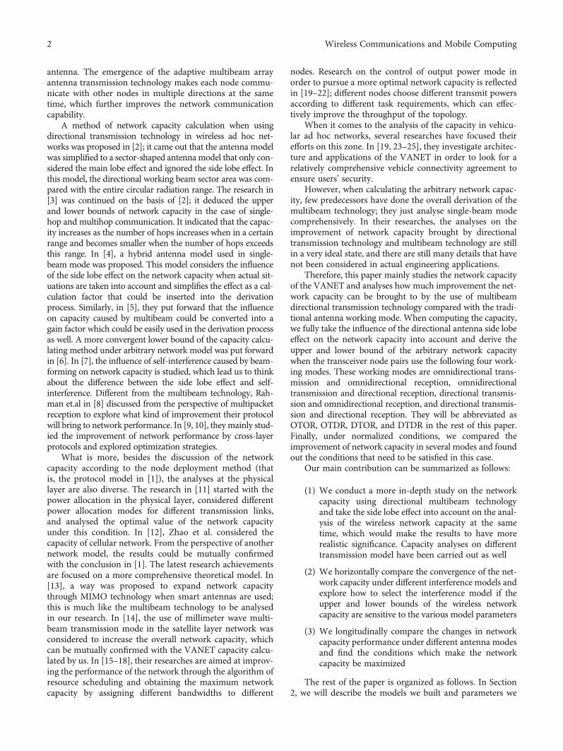
2.3.3. Interference Area Description. Now, let us calculate thearea of the interference region, which is an important part ofthe subsequent calculation work. As mentioned above, wederive the network capacity under four working modes:OTOR, OTDR, DTOR, and DTDR.

In Figure 2, compared to the OTOR working mode, theother three modes cover a longer distance in the beam direc-tion and a larger interference area.

First, we define two parameters; the parameter r men-tioned before refers to the antenna radiation radius in thedirectional transmission mode; what is more, the parameterξaða = 1, 2, 3, 4Þ indicates the ratio between the area of AOOand other three modes.

3Wireless Communications and Mobile Computing

For OTOR, the area of the interference region is

AOO = πr12 = πr1

2ξ1, ð3Þ

where r1 means the radius of the omnidirectional antennaradiation pattern.

For OTDR, the model is shown in Figure 2(a); taking thesingle-beam transmission mode, the area is

AOD1 = π srð Þ2 + θ

2ππr2 − π srð Þ2� �

= πr2 s2 + 1 − s2� � θ

2π

� = πr2ξ2:

ð4Þ

When the multibeam mode is adopted, since the numberof beams directed by the receiving node to the transmittingnode has not changed, the area has not changed.

For DTOR, the model is shown in Figure 2(b), and tak-ing the single-beam transmission mode, the area is

ADO1 = πr2P Xi − Xj

�� ≤ sr �

+ πr2P Xi − Xj

�� > sr �

· P Xi ⟶ Xj

�= πr2 s2 + 1 − s2

� � θ

2π

� = AOD1:

ð5Þ

Different from OTDR, the area has changed whenadopting multibeam mode in that the number of the receiv-ing beam has become m, and it changes to

ADOm = πr2P Xi − Xj

�� ≤ sr �

+ πr2P Xi − Xj

�� > sr �

· P Xi ⟶ Xj

�= πr2 s2 + 1 − s2

� �mθ

2π

� = πr2ξ3:

ð6Þ

Table 1: Symbols and parameters’ description.

Symbols and parameters Explanation

m Number of beams

λ Node transmission rate (bit/s)

η The gain of multibeam

T Total communication time

Γ The set of all nodes transmitting in the same channel simultaneously

C A constant determined by antenna heights, wavelength, and so on

d Euclidean distance between transmitting node and receiving node

α α ≥ 2 means path loss exponent

Gmain Main lobe gain

Gside Side lobe gain

s The ratio of the radius of Gside and Gmain in the hybrid antenna mode

N The ambient noise power level at the receiver

r nð Þ Node communication radius

�L Average distance from source to destination

β The minimum signal-to-interference plus noise ratio (SINR) for successful receptions at the receiver

h bð Þ Total number of hops required for the data-bit b to move from source to destination

Side lobe gain

Main lobe gain

Side lobe gain

Main lobe gain

θ

θ

θ

θ

Single beamtransmission

Multi-beamtransmission

Figure 1: Hybrid antenna model in directional transmission mode.


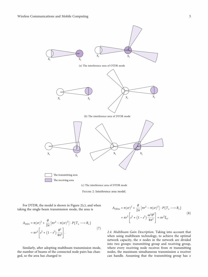
For DTDR, the model is shown in Figure 2(c), and whentaking the single-beam transmission mode, the area is

ADD1 = π srð Þ2 + θ


· P Tx ⟶ Rvf g

= πr2 s2 + 1 − s2� � θ2

4π2

" #:

ð7Þ

Similarly, after adopting multibeam transmission mode,the number of beams of the connected node pairs has chan-ged, so the area has changed to

ADDm = π srð Þ2 + θ


· P Tx ⟶ Rvf g

= πr2 s2 + 1 − s2� �m2θ2

4π2

" #= πr2ξ4:

ð8Þ

2.4. Multibeam Gain Description. Taking into account thatwhen using multibeam technology, to achieve the optimalnetwork capacity, the n nodes in the network are dividedinto two groups: transmitting group and receiving group,where every receiving node receives from m transmittingnodes, the maximum simultaneous transmission a receivercan handle. Assuming that the transmitting group has x

Xi

XiXj

Xj

(a) The interference area of OTDR mode

Xi XjXi

Xj

(b) The interference area of DTOR mode

Xi XjXi Xj

The transmitting area

The receiving area

(c) The interference area of DTDR mode

Figure 2: Interference area model.


nodes, then the receiving group has ðn − xÞ nodes. In OTORand DTDR modes, all nodes can be divided into two parts,half for transmission and half for reception. At this time,the OTOR gain equals to 1, and the DTDR gain is η =m.In the OTDR mode, the transmit flow is equal to the receiveflow, that is, xW = ðn − xÞmW; therefore, it can be con-cluded that the gain of network capacity at this time is η =ððnm/ðm + 1ÞÞW + ðn − ðnm/ðm + 1ÞÞÞmWÞ/nW = 2m/ðm+ 1Þ. Similarly, in the DTOR mode, it can be derived thatthe gain is equal to that in the OTDR mode.

3. The Upper Bound of ArbitraryNetwork Capacity

If the communication time is T seconds and the node trans-mission rate is λ bits per second, λnT bits of total data canbe transmitted. If the average distance from source to desti-nation is L, the whole topology can transmit λnL bit-metersper second.

In the following of this section, we may derive the upperbound of the network capacity based on the two interferencemodels proposed in the above section.

3.1. Using the Protocol Model of the Interference. Supposingbit b, where 1 ≤ b ≤ λnT , is moving from its source to thedestination with hðbÞ hops in T seconds, where the hthhop traverses the distance of rhb . Since the transmission dis-tance is at least equal to the total length of the path connect-ing the source with the destination, so we have

〠λnT

b=1〠h bð Þ

h=1rhb ≥ λnTL: ð9Þ

Before the subsequent derivation process is carried out,we introduce a new parameter H, which means the total

number of hops that all bits transmit in time T , i.e., H =∑λnT

b=1 hðbÞ. Therefore, the number of bits transmitted by allnodes in T seconds is equal to H. As mentioned in Section2.4, the gain in the multibeam mode is η, so

H = 〠λnT

b=1h bð Þ ≤ WTηn

2: ð10Þ

According to [1, 4], we can get that all nodes communi-cate in the same subchannel and time will not interfere witheach other if each hop consumes a disk of radius Δ/2 timesthe length of the hop around each receiver, i.e., rhb .

Considering the edge effect, if a neighbor node is close tothe edge of the area and noting that a range greater than thediameter of the domain is unnecessary, at least a quarter ofits interference circular area caused by the neighbor nodeis within the communication range. Within the same com-munication time period, at most WT bits of data flow can

be generated. Therefore, we can obtain that ∑λnTb=1∑

hðbÞh=1 ð1/4Þ

ðΔ/2Þ2 ·AI ≤ ηWT , and it can be rewritten as

〠λnT

b=1〠h bð Þ

h=1

rhb� �2H

≤16ηWT

π ξaΔ2H

: ð11Þ

Note that the quadratic function on the left side ofinequality (9) is convex, so we can get

〠λnT

b=1〠h bð Þ

h=1

rhbH

!2

≤ 〠λnT

b=1〠h bð Þ

h=1

rhb� �H

2

: ð12Þ

Combining expressions (9), (10), (11), and (12), theupper bound of the network capacity can be obtained as

Note that the result in OTOR mode is consistent withthe result obtained in [1].

3.2. Using the Physical Model of the Interference. The differ-ence from the protocol model is that in order to perform

subsequent calculations in the physical model, inequality(9) needs to be replaced with different expressions. Accord-ing to inequality (2), if the power of transmitting nodes isalso put into the entire set of the same time slot and onthe same subchannel, i.e., add the numerator on the left side

λnTL ≤2ηWT

Δ

ffiffiffiffiffiffiffi2nπξa

s=

2mWTΔ

ffiffiffiffiffiffiffiffiffiffiffiffiffiffiffiffiffiffiffiffiffiffiffiffiffiffiffiffiffiffiffiffiffiffiffiffiffiffiffiffiffiffiffiffiffiffiffiffiffiffiffiffi2n

π s2 + 1 − s2ð Þ m2θ2/4π2� ��

sthe capacity inDTDRmodeð Þ,

4mWTm + 1ð ÞΔ

ffiffiffiffiffiffiffiffiffiffiffiffiffiffiffiffiffiffiffiffiffiffiffiffiffiffiffiffiffiffiffiffiffiffiffiffiffiffiffiffiffiffiffiffiffi2n

π s2 + 1 − s2ð Þ mθ/2πð Þ½ �

sthe capacity inDTORmodeð Þ,

4mWTm + 1ð ÞΔ

ffiffiffiffiffiffiffiffiffiffiffiffiffiffiffiffiffiffiffiffiffiffiffiffiffiffiffiffiffiffiffiffiffiffiffiffiffiffiffiffiffi2n

π s2 + 1 − s2ð Þ θ/2πð Þ½ �

sthe capacity inOTDRmodeð Þ,

WTΔ

ffiffiffiffiffi8nπ

rthe capacity inOTORmodeð Þ:

8>>>>>>>>>>>>>>>>><>>>>>>>>>>>>>>>>>:

ð13Þ


of the inequality to the denominator, then (2) can be rewrit-ten as

PC GtGr/ Xi − Xj

�� α� �N +∑k∈Γ PC ·GtGr/ Xk − Xj

�� α� � ≥ β

β + 1: ð14Þ

Hence, we can get

Xi − Xj

�� α ≤ β + 1β

·PC ·GtGr

N +∑k∈Γ PC ·GtGr/ Xk − Xj

�� α� � : ð15Þ

Since the communication area is a disk of unit area, inother words, the area is 1; therefore, we can easily get π

ðjXi − Xjj/2Þ2 ≤ 1, jXi − Xjj ≤ 2/ffiffiffiπ

p. In addition, expression

(15) can be rewritten as jXi − Xjjα ≤ ððβ + 1Þ/βÞ · ððPC ·Gt

GrÞ/ðN + ðπ/4Þα/2 ·∑k∈ΓPC ·GtGrÞÞ.While summing all the transmitting and receiving nodes

in the same channel at this communicating time, we can get

〠i∈Γ

Xi − Xj

�� α ≤ β + 1β

· ∑i∈ΓPC · GtGr

N + π/4ð Þα/2 ·∑k∈ΓPC ·GtGr

=β + 1β

·1

N/ ∑i∈ΓPC · GtGrð Þð Þ + π/4ð Þα/2 ∑k∈ΓGtGr/∑i∈ΓGtGrð Þ

≤β + 1β

·4π

� α/2 ∑i∈ΓGtGr

∑k∈ΓGtGr:

ð16Þ

Due to different working modes, the antenna gains of thetransmitting and receiving pairs are also different. Therefore,

we use the parameter γa to characterize the ratio ∑i∈ΓGtGr/∑k∈ΓGtGr and it is

γa =∑i∈ΓGtGr

∑k∈ΓGtGr=

∑i∈ΓGsideGside∑k∈ΓGsideGside

= 1 inOTORmodeð Þ,

∑i∈ΓGsideGmain∑k∈ΓGsideGside

=1sinOTDRmodeð Þ,

∑i∈ΓGmainGside∑k∈ΓGsideGside

=1sinDTORmodeð Þ,

∑i∈ΓGmainGmain∑k∈ΓGsideGside

=1s2

inDTDRmodeð Þ:

8>>>>>>>>>>>>><>>>>>>>>>>>>>:

ð17Þ

Therefore, (13) can be rewritten as

〠i∈Γ

Xi − Xj

�� α ≤ β + 1β

·4π

� α/2γa: ð18Þ

It can be seen from the previous analysis that rhb = jXi

− Xjj. Therefore, by adding up the communication datastream in all subchannels of all time slots, an expression sim-ilar to inequality (9) can be obtained that

〠λnT

b=1〠h bð Þ

h=1

rhb� �H

α

≤β + 1ð Þ/βð Þ · 4/πð Þα/2γaηWT

Hξa: ð19Þ

And after the similar derivation process, we can get thecapacity that

4. The Lower Bound of the ArbitraryNetwork Capacity

We mainly focus on the lower bound of network capacity bygiving that the node throughput can be achieved in a specificscenario. Therefore, we fix the all pairs of transmitter-receiver combination, i.e., the direction of transmitting beamand receiving beam is determined and fixed, and differentnode deployment models are determined according to dif-

ferent working modes. From the previous section, we knowthat the area of the whole communication region is 1, whichmeans the radius is 1/

ffiffiffiπ

p. Then, we establish a rectangular

coordinate system on this circle, and the origin is the centerof the circle.

4.1. Network Capacity in OTOR Mode. Just like Figure 3, wewill place receivers at these locations: ðjð1 + 2ΔÞr ± Δr, kð1+ 2ΔÞrÞ and ðjð1 + 2ΔÞr, kð1 + 2ΔÞr ± ΔrÞ, if jj + kj is odd.

λnT�L ≤ηWTffiffiffi

πp 2β + 2ð Þnα−1γa

βξa

� 1/α=

mWTffiffiffiπ

p 2β + 2ð Þnα−1β s2 + 1 − s2ð Þ m2θ2/4π2� ��

s2

" #the capacity inDTDRmodeð Þ,

2mWT

m + 1ð Þ ffiffiffiπ

p 2β + 2ð Þnα−1β s2 + 1 − s2ð Þ mθ/2πð Þ½ �s�

the capacity inDTORmodeð Þ,

2mWT

m + 1ð Þ ffiffiffiπ

p 2β + 2ð Þnα−1β s2 + 1 − s2ð Þ θ/2πð Þ½ �s�

the capacity inOTDRmodeð Þ,

WTffiffiffiπ

p 2β + 2ð Þnα−1β

� the capacity inOTORmodeð Þ:

8>>>>>>>>>>>>>>><>>>>>>>>>>>>>>>:

ð20Þ


Then, we place transmitters at these locations ðjð1 + 2ΔÞr ± Δr, kð1 + 2ΔÞrÞ and ðjð1 + 2ΔÞr, kð1 + 2ΔÞr ± ΔrÞ if jj+ kj is even.

In the protocol model, all transmitters transmit to theirnearest receiver, and the transmission distance is r. On thiscondition, there is no interfering node in themiddle, and therewill be n/2 pairs of receivers and transmitters in the communi-cation area. Now, we define a new parameter L, and L = ð1+ 2ΔÞr, which means the side length of the square that nodesdeployed on. So according to [3], all such squares that intersectwith a disk of radius ðð1/ ffiffiffi

πp Þ − ffiffiffi

2p

LÞ are entirely contained inthe communication area; therefore, we can get that the num-

ber of these squares is at least ðπðð1/ ffiffiffiπ

p Þ − ffiffiffi2

pLÞ2Þ/L2. It

can be observed from Figure 3 that each square contains twopairs of transmitting and receiving nodes; hence,

π 1/ffiffiffiπ

p� �−

ffiffiffi2

pL

� �2L2

:2 =n2: ð21Þ

Then, we can derive that the communication radius is r= L/ð1 + 2ΔÞ = 2/ðð1 + 2ΔÞð ffiffiffiffiffiffi

8πp

+ffiffiffin

p ÞÞ, and it is equal tothe average distance between nodes according to our node’sdeployment strategy. Therefore, the capacity is

λnTL =Wn2Tr =

nWT

1 + 2Δð Þ ffiffiffin

p+

ffiffiffiffiffiffi8π

p� � : ð22Þ

Now, we turn to the physical model, according to expres-sion (2) and description of the link interference in the physicalmodel in [6], we give the relevant interference factor in pathtransmission, denoted by as, to be

as = β ·N +∑k∈Γ PC ·GtGr/ Xk − Xj

�� α� �PC GtGr/ Xi − Xj

�� α� � = β 1 +1

SINR

� = β

S + I +NS

,

ð23Þ

where S = PCðGtGr/jXi − XjjαÞ means the transmitted signalpower. Let c = ð1 + 2ΔÞ. It can be seen from Figure 3 that thedistance between any two transmitters ðSi, SjÞ is not less thanðc − 1Þ times the distance between the nearest transceiver pairðSi, RiÞ, that is, dðSi ,SjÞ ≥ ðc − 1ÞdðSi ,RiÞ = ðc − 1Þr.

Therefore, the circles of radius ððc − 1ÞrÞ/2 around thetransmitter do not intersect each other. We call the concentriccircles formed by nodes placed at the same distance from thecenter of the transmitter as Ringk, where k = 0, 1, 2⋯ . If k= 0, it means that there is no transmitter. The circle withradius ððc − 1ÞrÞ/2 around the transmitter also belongs to thislevel of concentric circle. The area of the kth concentric ring is

A Ringkð Þ = π k + 1ð Þcr + c − 1ð Þr2

� 2− kcr −

c − 1ð Þr2

� 2( )

= πc 2c − 1ð Þ 2k + 1ð Þr2:ð24Þ

Transmitters

Receivers

Figure 3: Node deployment model in OTOR mode.


Therefore, the interference caused by concentric rings ateach level is

Ik ≤ 〠Sw∈Ringk

ISw ≤A Ringkð Þ

π c − 1ð Þrð Þ/2½ �2 ·P

kcrð Þα

≤4Pc 2k + 1ð Þ 2c − 1ð Þ

cαrαkα c − 1ð Þ2 ≤253P

cαrαkα−1,

ð25Þ

where Sw indicates one node belongs to Ringk.Summing all interferences in the concentric rings, we get

Isum ≤ 〠∞

k=1Ik ≤ 〠

∞

k=1

253Pcαrαkα−1

<α − 1α − 2

253Pcαrα

: ð26Þ

Bring inequality (18) into equation (23), we can get

as = β 1 +1

SINR

� = β

S + Isum +NS

< βIsumS

≤α − 1α − 2

253βcα

:

ð27Þ

Therefore, we can obtain SINR ≥ 1/ðððα − 1Þ/ðα − 2ÞÞð96/cαÞ − 1Þ = 1/ðððα − 1Þ/ðα − 2ÞÞð96/ð1 + 2ΔÞαÞ − 1Þ, andsince SINRmin = β, additionally we can get

1 + 2Δð Þmax =96ββ + 1

α − 1α − 2

� 1/α: ð28Þ

Combining equation (28) with the expression of capac-ity, we can derive that the lower bound of the capacity inphysical model is

λnTL =Wn2Tr =

nWT

96β/ β + 1ð Þð Þ α − 1ð Þ/ α − 2ð Þð Þð Þ1/α ffiffiffin

p+


p� � :ð29Þ

4.2. Network Capacity in OTDR Mode. First of all, we willstill derive the lower bound of the capacity in the protocolmodel. Some parameters and their definitions ought to beclarified in that they will be reused. Let r1 = Δr/2, r2 = r +r1, and L = 4r2. Just like Section 4.1, we place transmittingnodes at these locations: ½pL + ðr + r1Þ cos ððπ/2Þ + ðð2i − 1Þ/mÞπÞ, qL + ðr + r1Þ sin ððπ/2Þ + ðð2i − 1Þ/mÞπÞ�, and placereceiving nodes at these locations: ½pL + r1 cos ððπ/2Þ + ðð2i− 1Þ/mÞπÞ, qL + r1 sin ððπ/2Þ + ðð2i − 1Þ/mÞπÞ�, where p, q,

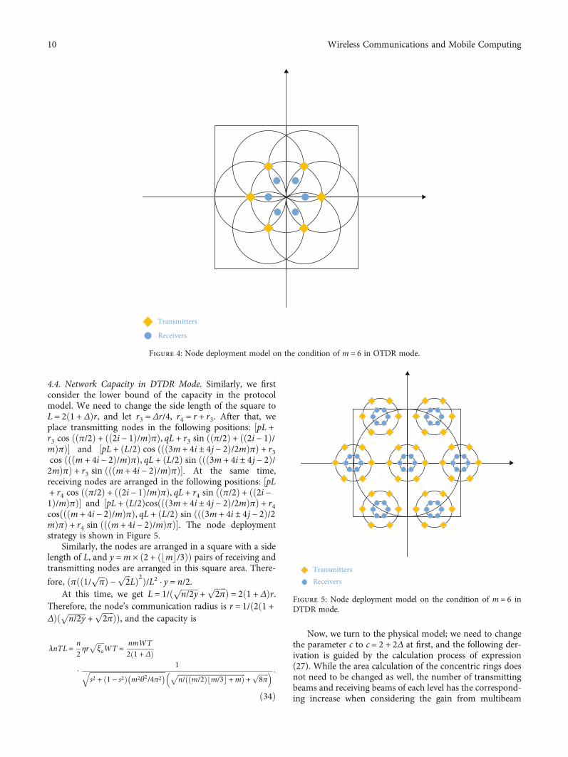
i, and j are integers and i ∈ ½0,m − 1�, j ∈ ½0,m/6�. The nodedeployment strategy is shown in Figure 4.

Similar to the derivation process in the above section, thenumber of transceiver pairs arranged in the square is chan-ged to m on this condition; therefore, its communicationradius should also change to r = 1/ðð4 + 2ΔÞð ffiffiffiffiffiffi

2πp

+ffiffiffiffiffiffiffiffiffiffiffin/2m

pÞÞ, and the capacity in this mode is

λnTL =n2ηffiffiffiffiffiξa

prWT

=nmWT

m + 1ð Þ 2 + Δð Þ·

1ffiffiffiffiffiffiffiffiffiffiffiffiffiffiffiffiffiffiffiffiffiffiffiffiffiffiffiffiffiffiffiffiffiffiffiffis2 + 1 − s2ð Þ θ/2πð Þp ffiffiffiffiffiffi

8πp

+ffiffiffiffiffiffiffiffiffiffiffi2n/m

p� � :ð30Þ

Now, we turn to the physical model; the derivation pro-cess is carried on according to expression (23) as well. Letparameter c change into c = ð4 + 2ΔÞ. While we do not needto change the area calculation method of each concentricring level, the interference in each level that needs to con-sider further is the directional gain, i.e.,


ISw ≤A Ringkð Þ

π c − 1ð Þrð Þ/2½ �2 ·PGmainkcrð Þα

≤4Pc 2k + 1ð Þ 2c − 1ð ÞGmain

cαrαkα c − 1ð Þ2 ≤253PGmain

cαrαkα−1:

ð31Þ

Therefore, the corresponding changes need to be takeninto consideration, and finally, we can obtain the lowerbound of the capacity in this mode that


prWT

=nmWT

m + 1ð Þ 96Gmainβ/ β + 1ð Þð Þ α − 1ð Þ/ α − 2ð Þð Þð Þ1/α

·1ffiffiffiffiffiffiffiffiffiffiffiffiffiffiffiffiffiffiffiffiffiffiffiffiffiffiffiffiffiffiffiffiffiffiffiffi

s2 + 1 − s2ð Þ θ/2πð Þp ffiffiffiffiffiffi8π

p+

ffiffiffiffiffiffiffiffiffiffiffi2n/m

p� � :ð32Þ

4.3. Network Capacity in DTOR Mode. We can obtain thesame conclusion by swapping the transmitter and receiverpositions in Section 4.2, and the result is similar to expres-sions (30) and (32); they are


prWT =

nmWTm + 1ð Þ 2 + Δð Þ ·

1ffiffiffiffiffiffiffiffiffiffiffiffiffiffiffiffiffiffiffiffiffiffiffiffiffiffiffiffiffiffiffiffiffiffiffiffiffiffiffis2 + 1 − s2ð Þ mθ/2πð Þp ffiffiffiffiffiffi

8πp


p� � if in the protocolmodelð Þ,

nmWT

m + 1ð Þ 96Gmainβ/ β + 1ð Þð Þ α − 1ð Þ/ α − 2ð Þð Þð Þ1/α·

1ffiffiffiffiffiffiffiffiffiffiffiffiffiffiffiffiffiffiffiffiffiffiffiffiffiffiffiffiffiffiffiffiffiffiffiffiffiffiffis2 + 1 − s2ð Þ mθ/2πð Þp ffiffiffiffiffiffi

8πp


p� � if in the physicalmodelð Þ:

8>>>>><>>>>>:

ð33Þ


4.4. Network Capacity in DTDR Mode. Similarly, we firstconsider the lower bound of the capacity in the protocolmodel. We need to change the side length of the square toL = 2ð1 + ΔÞr, and let r3 = Δr/4, r4 = r + r3. After that, weplace transmitting nodes in the following positions: ½pL +r3 cos ððπ/2Þ + ðð2i − 1Þ/mÞπÞ, qL + r3 sin ððπ/2Þ + ðð2i − 1Þ/mÞπÞ� and ½pL + ðL/2Þ cos ððð3m + 4i ± 4j − 2Þ/2mÞπÞ + r3cos ðððm + 4i − 2Þ/mÞπÞ, qL + ðL/2Þ sin ððð3m + 4i ± 4j − 2Þ/2mÞπÞ + r3 sin ðððm + 4i − 2Þ/mÞπÞ�. At the same time,receiving nodes are arranged in the following positions: ½pL+ r4 cos ððπ/2Þ + ðð2i − 1Þ/mÞπÞ, qL + r4 sin ððπ/2Þ + ðð2i −1Þ/mÞπÞ� and ½pL + ðL/2Þcosððð3m + 4i ± 4j − 2Þ/2mÞπÞ + r4cosðððm + 4i − 2Þ/mÞπÞ, qL + ðL/2Þ sin ððð3m + 4i ± 4j − 2Þ/2mÞπÞ + r4 sin ðððm + 4i − 2Þ/mÞπÞ�. The node deploymentstrategy is shown in Figure 5.

Similarly, the nodes are arranged in a square with a sidelength of L, and y =m × ð2 + ðbmc/3ÞÞ pairs of receiving andtransmitting nodes are arranged in this square area. There-

fore, ðπðð1/ ffiffiffiπ

p Þ − ffiffiffi2

pLÞ2Þ/L2 · y = n/2.

At this time, we get L = 1/ð ffiffiffiffiffiffiffiffiffin/2y

p+


p Þ = 2ð1 + ΔÞr.Therefore, the node’s communication radius is r = 1/ð2ð1 +ΔÞð ffiffiffiffiffiffiffiffiffi

n/2yp

+ffiffiffiffiffiffi2π

p ÞÞ, and the capacity is

λnTL =n2ηr

ffiffiffiffiffiξa

pWT =

nmWT2 1 + Δð Þ

· 1ffiffiffiffiffiffiffiffiffiffiffiffiffiffiffiffiffiffiffiffiffiffiffiffiffiffiffiffiffiffiffiffiffiffiffiffiffiffiffiffiffiffiffiffiffis2 + 1 − s2ð Þ m2θ2/4π2

� �q ffiffiffiffiffiffiffiffiffiffiffiffiffiffiffiffiffiffiffiffiffiffiffiffiffiffiffiffiffiffiffiffiffiffiffiffiffiffiffiffin/ m/2ð Þ m/3b c +mð Þp

+ffiffiffiffiffiffi8π

p� � :ð34Þ

Now, we turn to the physical model; we need to changethe parameter c to c = 2 + 2Δ at first, and the following der-ivation is guided by the calculation process of expression(27). While the area calculation of the concentric rings doesnot need to be changed as well, the number of transmittingbeams and receiving beams of each level has the correspond-ing increase when considering the gain from multibeam

Transmitters

Receivers

Figure 4: Node deployment model on the condition of m = 6 in OTDR mode.

TransmittersReceivers

Figure 5: Node deployment model on the condition of m = 6 inDTDR mode.


technology. Therefore, the number of transmitted signals ineach level of the ring also needs to be changed. What ismore, on the condition that the number of transmit beamsand the directional gain of the transmitting and receivinghave changed, the interference of each level also needs tobe changed to


ISw ≤A Ringkð Þ

π c − 1ð Þrð Þ/2½ �2 ·mPG2

mainkcrð Þα

≤4Pmc 2k + 1ð Þ 2c − 1ð ÞG2

main

cαrαkα c − 1ð Þ2

≤253mPG2

main

cαrαkα−1:

ð35Þ

The subsequent derivation is similar to the process inSection 4.1, so the capacity is

λnTL =n2ηr

ffiffiffiffiffiξa

pWT

=nmWT

96βmG2main/ β + 1ð Þ� �

α − 1ð Þ/ α − 2ð Þð Þ� �1/α· 1ffiffiffiffiffiffiffiffiffiffiffiffiffiffiffiffiffiffiffiffiffiffiffiffiffiffiffiffiffiffiffiffiffiffiffiffiffiffiffiffiffiffiffiffiffi

s2 + 1 − s2ð Þ m2θ2/4π2� �q ffiffiffiffiffiffiffiffiffiffiffiffiffiffiffiffiffiffiffiffiffiffiffiffiffiffiffiffiffiffiffiffiffiffiffiffiffiffiffiffi

n/ m/2ð Þ m/3b c +mð Þp+


p� � :ð36Þ

5. Mathematical Analysis

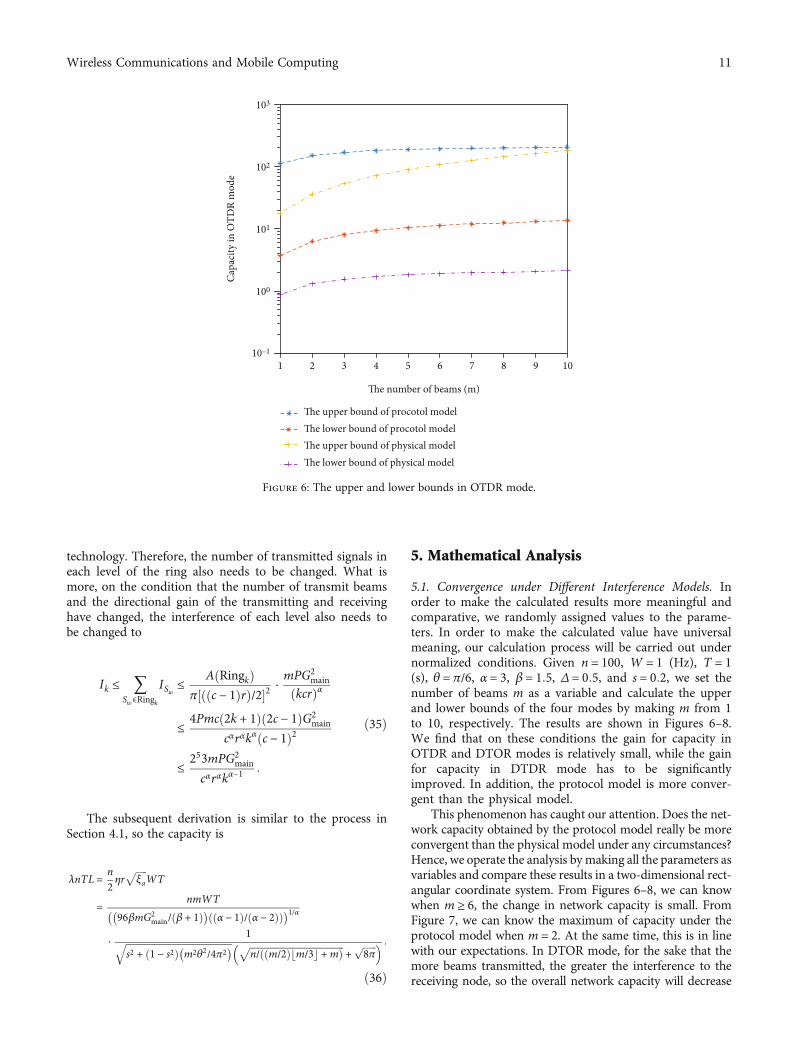
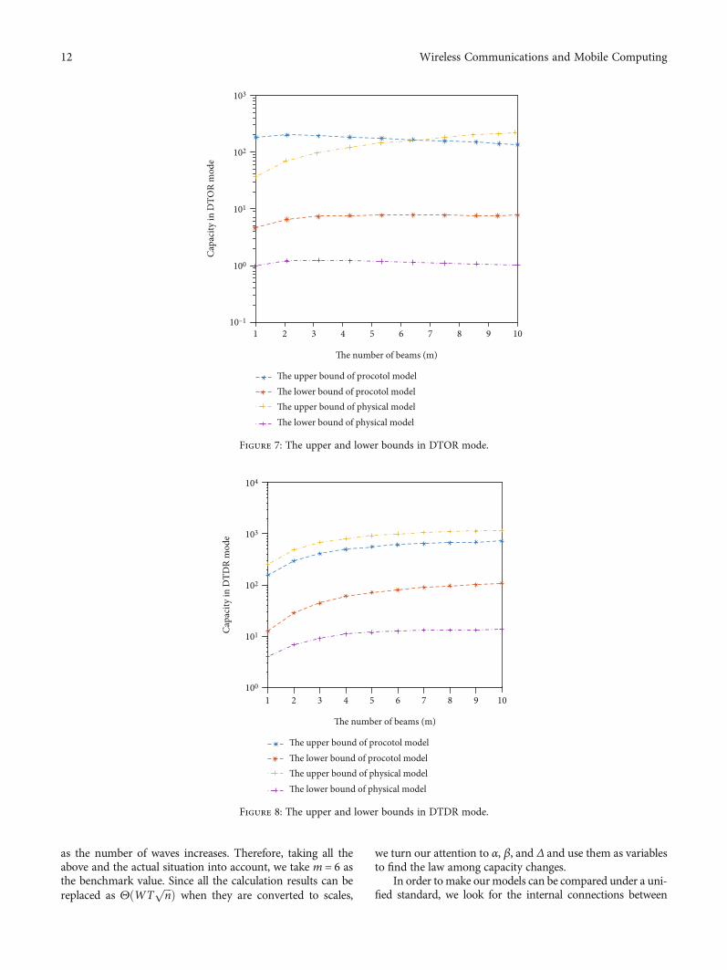
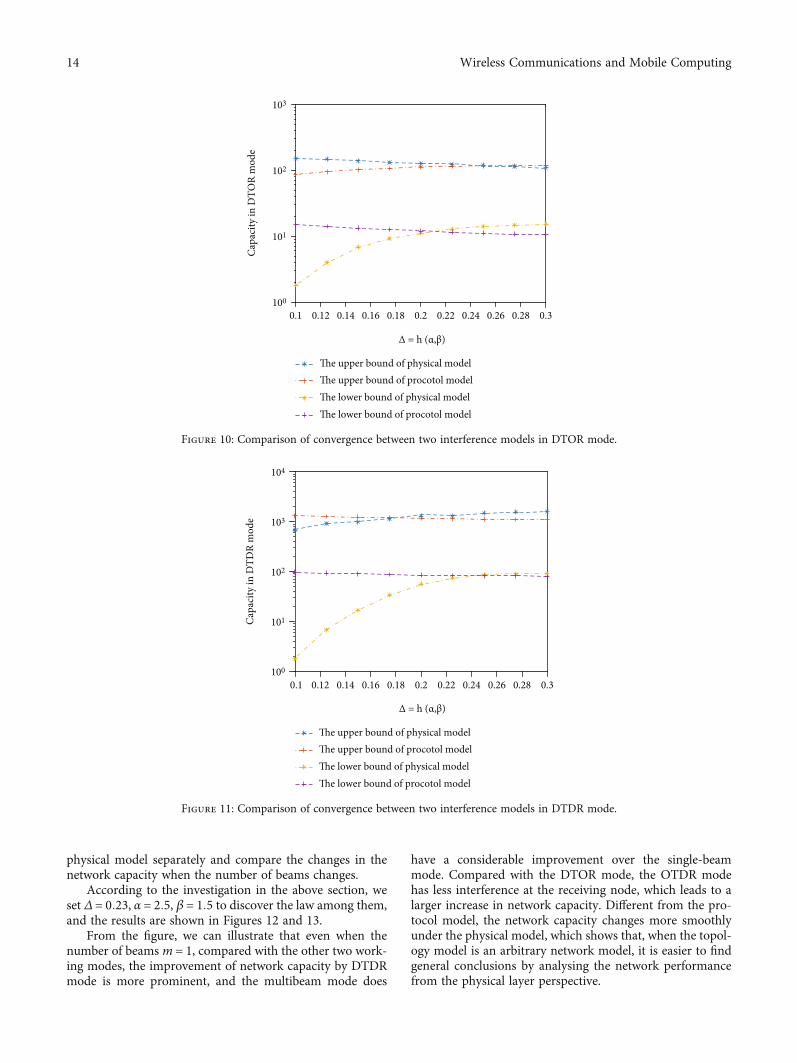
5.1. Convergence under Different Interference Models. Inorder to make the calculated results more meaningful andcomparative, we randomly assigned values to the parame-ters. In order to make the calculated value have universalmeaning, our calculation process will be carried out undernormalized conditions. Given n = 100, W = 1 (Hz), T = 1(s), θ = π/6, α = 3, β = 1:5, Δ = 0:5, and s = 0:2, we set thenumber of beams m as a variable and calculate the upperand lower bounds of the four modes by making m from 1to 10, respectively. The results are shown in Figures 6–8.We find that on these conditions the gain for capacity inOTDR and DTOR modes is relatively small, while the gainfor capacity in DTDR mode has to be significantlyimproved. In addition, the protocol model is more conver-gent than the physical model.

This phenomenon has caught our attention. Does the net-work capacity obtained by the protocol model really be moreconvergent than the physical model under any circumstances?Hence, we operate the analysis by making all the parameters asvariables and compare these results in a two-dimensional rect-angular coordinate system. From Figures 6–8, we can knowwhen m ≥ 6, the change in network capacity is small. FromFigure 7, we can know the maximum of capacity under theprotocol model when m = 2. At the same time, this is in linewith our expectations. In DTOR mode, for the sake that themore beams transmitted, the greater the interference to thereceiving node, so the overall network capacity will decrease

1 2 3 4 5 6 7 8 9 10

The number of beams (m)

Capa

city

in O

TDR

mod

e

The upper bound of procotol modelThe lower bound of procotol modelThe upper bound of physical modelThe lower bound of physical model

10–1

100

101

102

103

Figure 6: The upper and lower bounds in OTDR mode.


as the number of waves increases. Therefore, taking all theabove and the actual situation into account, we take m = 6 asthe benchmark value. Since all the calculation results can bereplaced as ΘðWT

ffiffiffin

p Þ when they are converted to scales,

we turn our attention to α, β, and Δ and use them as variablesto find the law among capacity changes.

In order to make ourmodels can be compared under a uni-fied standard, we look for the internal connections between

1 2 3 4 5 6 7 8 9 10


Capa

city

in D

TDR

mod

e

100

101

102

103

104


Figure 8: The upper and lower bounds in DTDR mode.

Capa

city

in D

TOR

mod

e

1 2 3 4 5 6 7 8 9 10


10–1

100

101

102

103


Figure 7: The upper and lower bounds in DTOR mode.


variables. In the derivation process, we found that there is amutual transformation relationship betweenΔ and α, β. There-fore, we use the parameter Δ in the protocol model as a refer-ence variable to look for changes of capacity in differentinterference models.

The analysis of the upper bound is first carried out. Wecompare the capacity of the physical model when 2 < α ≤ 5and 1 < β ≤ 3 with the capacity of the protocol model when0:1 ≤ Δ ≤ 0:3, and the results are shown in Figures 9–11.We use

to represent the transformation relationship between α, βand Δ, and the proof of correlation between parameterscan be referenced in [1, 3, 6, 9]. It is found that in the OTDRand DTDR mode when Δ ≤ 0:22, using the physical modelcan make the calculated value more convergent and whenΔ ≤ 0:26 in the DTOR mode the physical model can makethe calculated value more convergent. In other cases, it isthe protocol model that makes the derived theoretical valueof capacity more convergent.

The next is the analysis of the lower bound. It can be seenthat in the OTDR and DTDR mode when Δ ≥ 0:24 using thephysical model can make the calculated value more conver-gent and in the DTOR mode when Δ ≥ 0:22 the physicalmodel can make the calculated value more convergent.

In actual application, due to the influence of the transmis-sion medium and the electromagnetic environment, the pathtransmission loss α is generally a certain constant, and theradius of the protected area will not exceed 0:3 times the com-munication radius, i.e., Δ ≤ 0:3, d ≤ ð1 + 0:3Þr. And becausewe usually find the maximum network capacity in actual engi-neering, based on the above analysis, we conclude that whenΔ ≤ 0:23, we try to choose the protocol model as the measure-ment method; otherwise, we choose the physical model.

5.2. Capacity Improvement Based on Directional MultibeamTransmission. For the evaluation of network performanceimprovement, we only analyse the upper bound of the net-work capacity. We investigate the protocol model and the

0.1 0.12 0.14 0.16 0.18 0.2 0.22 0.24 0.26 0.28 0.3

Δ = h (α,β)

Capa

city

in O

TDR

mod

e

100

101

102

103

The upper bound of procotol model

The lower bound of procotol model

The upper bound of physical model

The lower bound of physical model

Figure 9: Comparison of convergence between two interference models in OTDR mode.

Δ = h α, βð Þ =

βPminβ + 1ð ÞPmax

� 1/α− 1 in all upper bound calculationsð Þ,

96βGmain α − 1ð Þβ + 1ð Þ α − 2ð Þ

� 1/α− 2 in the lower bound of OTDR andDTORmodeð Þ,

96βG2main α − 1ð Þ

β + 1ð Þ α − 2ð Þ� 1/α

− 1 in the lower bound of DTDRmodeð Þ,

8>>>>>>>>><>>>>>>>>>:

ð37Þ


physical model separately and compare the changes in thenetwork capacity when the number of beams changes.

According to the investigation in the above section, weset Δ = 0:23, α = 2:5, β = 1:5 to discover the law among them,and the results are shown in Figures 12 and 13.

From the figure, we can illustrate that even when thenumber of beams m = 1, compared with the other two work-ing modes, the improvement of network capacity by DTDRmode is more prominent, and the multibeam mode does

have a considerable improvement over the single-beammode. Compared with the DTOR mode, the OTDR modehas less interference at the receiving node, which leads to alarger increase in network capacity. Different from the pro-tocol model, the network capacity changes more smoothlyunder the physical model, which shows that, when the topol-ogy model is an arbitrary network model, it is easier to findgeneral conclusions by analysing the network performancefrom the physical layer perspective.

0.1 0.12 0.14 0.16 0.18 0.2 0.22 0.24 0.26 0.28 0.3

Capa

city

in D

TDR

mod

e

Δ = h (α,β)

100

102

101

103

104





Figure 11: Comparison of convergence between two interference models in DTDR mode.

0.1 0.12 0.14 0.16 0.18 0.2 0.22 0.24 0.26 0.28 0.3

Capa

city

in D

TOR

mod

e

Δ = h (α,β)





100

102

101

103

Figure 10: Comparison of convergence between two interference models in DTOR mode.


5.3. Capacity Optimization Strategy. The purpose of ouranalysis for the network capacity improvement degree is toachieve the goal that capacity optimized to the maximumby adjusting the equipment from the VANET node in mostscenarios. Since the path loss index α is fixed, the number ofbeams m is determined by the beam angle θ, the only twoparameters that can be adjusted are the beam angle θ andthe receiver SINR threshold β. Therefore, we study the rela-

tionship between capacity and these two parameters, and theresults are shown in Figures 14 and 15.

Since the receiver SINR threshold β is only reflected inthe capacity expression of the physical model, we only ana-lyse the relationship between the network capacity and βunder the physical model. Therefore, when studying therelationship between beam angle and capacity, we only ana-lyse the situation in the protocol model. As we can get from

1 2 3 4 5 6 7 8


0

2

4

6

8

10

12

The i

mpr

ovem

ent o

f cap

acity

in p

hysic

al m

odel

The improvement of OTDR modeThe improvement of DTOR modeThe improvement of DTDR mode

Figure 13: The improvement of network capacity by different working modes under the physical model.

1 2 3 4 5 6 7 8


2

3

4

5

6

7

8

The i

mpr

ovem

ent o

f cap

acity

in p

roto

col m

odel

The improvement of OTDR modeThe improvement of DTOR modeThe improvement of DTDR mode

Figure 12: The improvement of network capacity by different working modes under the protocol model.


1.1 1.2 1.3 1.4 1.5 1.6 1.7 1.8 1.9 2

The receiver SINR threshold β

200

300

400

500

600

700

800

The t

rans

miss

ion

capa

city

in th

e phy

sical

mod

el

The capacity in DTDR modeThe capacity in DTOR mode

The capacity in OTDR modeThe capacity in OTOR mode

Figure 14: The relationship between the receiver SINR threshold β and the VANET capacity.

10 15 20 25 30 35 40 45 50 55

The beam angle θ (°)

101

102

103

The t

rans

miss

ion

capa

city

in th

e pro

toco

l mod

el

The capacity in DTDR modeThe capacity in DTOR mode

The capacity in OTDR modeThe capacity in OTOR mode

Figure 15: The relationship between the beam angle and the VANET capacity.


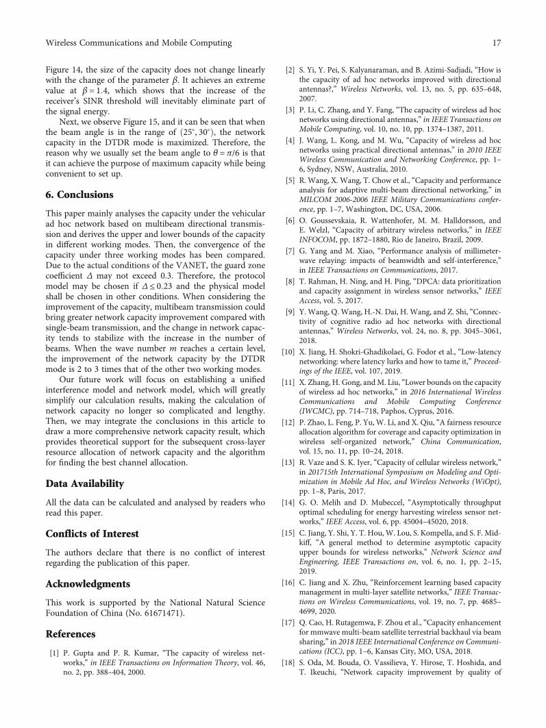
Figure 14, the size of the capacity does not change linearlywith the change of the parameter β. It achieves an extremevalue at β = 1:4, which shows that the increase of thereceiver’s SINR threshold will inevitably eliminate part ofthe signal energy.

Next, we observe Figure 15, and it can be seen that whenthe beam angle is in the range of ð25°, 30°Þ, the networkcapacity in the DTDR mode is maximized. Therefore, thereason why we usually set the beam angle to θ = π/6 is thatit can achieve the purpose of maximum capacity while beingconvenient to set up.

6. Conclusions

This paper mainly analyses the capacity under the vehicularad hoc network based on multibeam directional transmis-sion and derives the upper and lower bounds of the capacityin different working modes. Then, the convergence of thecapacity under three working modes has been compared.Due to the actual conditions of the VANET, the guard zonecoefficient Δ may not exceed 0.3. Therefore, the protocolmodel may be chosen if Δ ≤ 0:23 and the physical modelshall be chosen in other conditions. When considering theimprovement of the capacity, multibeam transmission couldbring greater network capacity improvement compared withsingle-beam transmission, and the change in network capac-ity tends to stabilize with the increase in the number ofbeams. When the wave number m reaches a certain level,the improvement of the network capacity by the DTDRmode is 2 to 3 times that of the other two working modes.

Our future work will focus on establishing a unifiedinterference model and network model, which will greatlysimplify our calculation results, making the calculation ofnetwork capacity no longer so complicated and lengthy.Then, we may integrate the conclusions in this article todraw a more comprehensive network capacity result, whichprovides theoretical support for the subsequent cross-layerresource allocation of network capacity and the algorithmfor finding the best channel allocation.

Data Availability

All the data can be calculated and analysed by readers whoread this paper.

Conflicts of Interest

The authors declare that there is no conflict of interestregarding the publication of this paper.

Acknowledgments

This work is supported by the National Natural ScienceFoundation of China (No. 61671471).

References

[1] P. Gupta and P. R. Kumar, “The capacity of wireless net-works,” in IEEE Transactions on Information Theory, vol. 46,no. 2, pp. 388–404, 2000.

[2] S. Yi, Y. Pei, S. Kalyanaraman, and B. Azimi-Sadjadi, “How isthe capacity of ad hoc networks improved with directionalantennas?,” Wireless Networks, vol. 13, no. 5, pp. 635–648,2007.

[3] P. Li, C. Zhang, and Y. Fang, “The capacity of wireless ad hocnetworks using directional antennas,” in IEEE Transactions onMobile Computing, vol. 10, no. 10, pp. 1374–1387, 2011.

[4] J. Wang, L. Kong, and M. Wu, “Capacity of wireless ad hocnetworks using practical directional antennas,” in 2010 IEEEWireless Communication and Networking Conference, pp. 1–6, Sydney, NSW, Australia, 2010.

[5] R. Wang, X. Wang, T. Chow et al., “Capacity and performanceanalysis for adaptive multi-beam directional networking,” inMILCOM 2006-2006 IEEE Military Communications confer-ence, pp. 1–7, Washington, DC, USA, 2006.

[6] O. Goussevskaia, R. Wattenhofer, M. M. Halldorsson, andE. Welzl, “Capacity of arbitrary wireless networks,” in IEEEINFOCOM, pp. 1872–1880, Rio de Janeiro, Brazil, 2009.

[7] G. Yang and M. Xiao, “Performance analysis of millimeter-wave relaying: impacts of beamwidth and self-interference,”in IEEE Transactions on Communications, 2017.

[8] T. Rahman, H. Ning, and H. Ping, “DPCA: data prioritizationand capacity assignment in wireless sensor networks,” IEEEAccess, vol. 5, 2017.

[9] Y. Wang, Q. Wang, H.-N. Dai, H. Wang, and Z. Shi, “Connec-tivity of cognitive radio ad hoc networks with directionalantennas,” Wireless Networks, vol. 24, no. 8, pp. 3045–3061,2018.

[10] X. Jiang, H. Shokri-Ghadikolaei, G. Fodor et al., “Low-latencynetworking: where latency lurks and how to tame it,” Proceed-ings of the IEEE, vol. 107, 2019.

[11] X. Zhang, H. Gong, andM. Liu, “Lower bounds on the capacityof wireless ad hoc networks,” in 2016 International WirelessCommunications and Mobile Computing Conference(IWCMC), pp. 714–718, Paphos, Cyprus, 2016.

[12] P. Zhao, L. Feng, P. Yu, W. Li, and X. Qiu, “A fairness resourceallocation algorithm for coverage and capacity optimization inwireless self-organized network,” China Communication,vol. 15, no. 11, pp. 10–24, 2018.

[13] R. Vaze and S. K. Iyer, “Capacity of cellular wireless network,”in 201715th International Symposium on Modeling and Opti-mization in Mobile Ad Hoc, and Wireless Networks (WiOpt),pp. 1–8, Paris, 2017.

[14] G. O. Melih and D. Mubeccel, “Asymptotically throughputoptimal scheduling for energy harvesting wireless sensor net-works,” IEEE Access, vol. 6, pp. 45004–45020, 2018.

[15] C. Jiang, Y. Shi, Y. T. Hou,W. Lou, S. Kompella, and S. F. Mid-kiff, “A general method to determine asymptotic capacityupper bounds for wireless networks,” Network Science andEngineering, IEEE Transactions on, vol. 6, no. 1, pp. 2–15,2019.

[16] C. Jiang and X. Zhu, “Reinforcement learning based capacitymanagement in multi-layer satellite networks,” IEEE Transac-tions on Wireless Communications, vol. 19, no. 7, pp. 4685–4699, 2020.

[17] Q. Cao, H. Rutagemwa, F. Zhou et al., “Capacity enhancementfor mmwave multi-beam satellite terrestrial backhaul via beamsharing,” in 2018 IEEE International Conference on Communi-cations (ICC), pp. 1–6, Kansas City, MO, USA, 2018.

[18] S. Oda, M. Bouda, O. Vassilieva, Y. Hirose, T. Hoshida, andT. Ikeuchi, “Network capacity improvement by quality of


transmission estimator with learning process,” in 2017 Euro-pean Conference on Optical Communication (ECOC), Gothen-burg, Sweden, 2017.

[19] X. Ma, H. Lu, J. Zhao, Y. Wang, J. Li, and M. Ni, “Commentson interference-based capacity analysis of vehicular ad hocnetworks,” IEEE Communications Letters, vol. 21, no. 10,pp. 2322–2325, 2017.

[20] Z. Wei, Z. Wang, X. Yuan, H. Wu, and Z. Feng, “Informationdensity–based energy-limited capacity of ad hoc networks,”International Journal of Distributed Sensor Networks, vol. 14,no. 4, 2018.

[21] B. Yang, Z. Wu, Y. Fan, X. Jiang, and S. Shen, “Non-asymptoticcapacity study in multicast mobile ad hoc networks,” IEEEAccess, vol. 7, pp. 115109–115121, 2019.

[22] S. Haddad and O. Leveque,On the Broadcast Capacity of LargeWireless Networks at Low SNR, IEEE, 2015.

[23] K. Raissi and B. B. Gouissem, “Hybrid communication archi-tecture in VANETs via named data network,” InternationalJournal of Communication Systems, vol. 34, no. 11, 2021.

[24] T. Yeferny and S. Hamad, “Vehicular ad-hoc networks: archi-tecture, applications and challenges,” International Journal ofComputer Science and Network Security, vol. 20, no. 2, 2020.

[25] S. More, R. Sonkamble, U. Naik, S. Phansalkar, P. More, andB. S. Saini, “Secured communication in vehicular adhoc net-works (VANETs) using blockchain,” IOP Conference Series:Materials Science and Engineering, vol. 1022, no. 1, article012067, 2021.


capacity of vehicular ad hoc networks based on multibeam

Documents