doi.org/10.26434/chemrxiv.7187540.v1

CANDOCK: Chemical Atomic Network Based Hierarchical FlexibleDocking Algorithm Using Generalized Statistical PotentialsJonathan Fine, Janez Konc, Ram Samudralal, Gaurav Chopra

Submitted date: 14/10/2018 • Posted date: 15/10/2018Licence: CC BY 4.0Citation information: Fine, Jonathan; Konc, Janez; Samudralal, Ram; Chopra, Gaurav (2018): CANDOCK:Chemical Atomic Network Based Hierarchical Flexible Docking Algorithm Using Generalized StatisticalPotentials. ChemRxiv. Preprint.

Small molecule docking has proven to be invaluable for drug design and discovery. However, existing dockingmethods have several limitations, such as, ignoring interactions with essential components in the chemicalenvironment of the binding pocket (e.g. cofactors, metal-ions, etc.), incomplete sampling of chemicallyrelevant ligand conformational space, and they are unable to consistently correlate docking scores of the bestbinding pose with experimental binding affinities. We present CANDOCK, a novel docking algorithm thatutilizes a hierarchical approach to reconstruct ligands from an atomic grid using graph theory and generalizedstatistical potential functions to sample chemical relevant ligand conformations. Our algorithm accounts forprotein flexibility, solvent, metal ions and cofactors interactions in the binding pocket that are traditionallyignored by current methods. We evaluate the algorithm on the PDBbind and Astex proteins to show its abilityto reproduce the binding mode of the ligands that is independent of the initial ligand conformation in thesebenchmarks. Finally, we identify the best selector and ranker potential functions, such that, the statisticalscore of best selected docked pose correlates with the experimental binding affinities of the ligands for anygiven protein target. Our results indicate that CANDOCK is a generalized flexible docking method thataddresses several limitations of current docking methods by considering all interactions in the chemicalenvironment of a binding pocket for correlating the best docked pose with biological activity.

File list (2)

download fileview on ChemRxiv2018_Fine-Konc_candock.pdf (3.83 MiB)

download fileview on ChemRxiv2018_Fine-Konc_candock_SI.pdf (3.89 MiB)

CANDOCK: Chemical atomic network based hierarchical flexible docking algorithm using generalized statistical potentials

Jonathan Fine1, ‡, Janez Konc2, ‡, Ram Samudrala3, Gaurav Chopra1,4,5,6,7 *

1Department of Chemistry, Purdue University, 720 Clinic Drive, West Lafayette, IN 47906

2National Institute of Chemistry, Hajdrihova 19, SI−1000, Ljubljana, Slovenia

3Department of Biomedical Informatics, SUNY, Buffalo, NY, USA

4Purdue Institute for Drug Discovery

5Purdue Center for Cancer Research

6Purdue Institute for Inflammation, Immunology and Infectious Disease

7Purdue Institute for Integrative Neuroscience

‡These authors share equal contribution to this work.

*Corresponding Author

E-mail: gchopra@purdue.edu

Abstract

Small molecule docking has proven to be invaluable for drug design and discovery. However, existing

docking methods have several limitations, such as, ignoring interactions with essential components in

the chemical environment of the binding pocket (e.g. cofactors, metal-ions, etc.), incomplete sampling

of chemically relevant ligand conformational space, and they are unable to consistently correlate

docking scores of the best binding pose with experimental binding affinities. We present CANDOCK, a

novel docking algorithm that utilizes a hierarchical approach to reconstruct ligands from an atomic grid

using graph theory and generalized statistical potential functions to sample chemical relevant ligand

conformations. Our algorithm accounts for protein flexibility, solvent, metal ions and cofactors

interactions in the binding pocket that are traditionally ignored by current methods. We evaluate the

algorithm on the PDBbind and Astex proteins to show its ability to reproduce the binding mode of the

ligands that is independent of the initial ligand conformation in these benchmarks. Finally, we identify

the best selector and ranker potential functions, such that, the statistical score of best selected docked

pose correlates with the experimental binding affinities of the ligands for any given protein target. Our

results indicate that CANDOCK is a generalized flexible docking method that addresses several

limitations of current docking methods by considering all interactions in the chemical environment of a

binding pocket for correlating the best docked pose with biological activity.

1. Introduction

Computational docking provides a means to predict and assess interactions between ligands and

proteins with relatively little investment. Application to proteins involved in disease holds the promise

of discovering new drug therapeutics. After decades of method development and application, this

promise has not been fully realized. The CANDOCK algorithm confronts several outstanding technical

and practical problems in computational docking. One significant problem is assessing goodness-of-fit,

or the likelihood that the given pose is the most physically realistic (native-like) pose among many

unrealistic binding poses. Another significant limitation is the lack of full protein flexibility in the

docking methods used today. The induced fit is a widely recognized challenge in computational drug

screening, where the protein and the ligand undergo conformational changes upon ligand binding.

Therefore, the traditional treatment of proteins as rigid structures is insufficient and often misleading

for structure-guided drug screening and design. Docking ligands to their protein targets is particularly

challenging when attempting to reproduce the binding mode of small molecules to ligand-free or

alternative ligand-bound protein structures, which invariably occurs in the practical application of any

docking method. Specifically, docking with ligand-bound (holo) protein structures typically leads to an

accuracy of 60-80%, whereas ligand-free (apo) structures yields a docking accuracy of merely 20-

40%1–5.

Several methods have been implemented to account for protein and ligand flexibility, including

multiple experimentally derived structures from X-ray crystallography6, nuclear magnetic resonance6

rotamer libraries7,8, Monte Carlo9,10, and molecular mechanics11,12. The same principle limits use of

multiple experimentally derived protein structures or side-chain rotamer libraries: binding a ligand to a

protein can cause conformational changes in either molecule that are not captured by these methods13.

The sampling problem is compounded by the fact that the protein main chain torsion angles are

also frequently altered from their ligand-free conformations, which these methods fail to capture.

Molecular mechanics is well suited for capturing fine detail side-chain and main chain motions and

rearrangements through energy minimization. However, molecular mechanics is limited in that

adequate sampling of all degrees of freedom between protein and ligand: rotation, translation, and

torsion angle are frequently computationally intractable. Further, the use of molecular dynamics has

been shown to disrupt the ligand from its native pose14.

Modern docking methods address these issues by employing algorithms such as the Genetic

Algorithm15–18 to sample the conformational space flexibly. However, it has been shown that these

methods do not adequately produce poses that rank the activity of the ligand well17,19 and that the

ability of these methods to produce a correct pose is dependent on the starting conformation of the

ligand in question20,21. Some methodologies use a fragment-based approach to docking22 to sample the

conformational space for a given ligand efficiently. These fragment-based methods have reported a

greater ability to rank activity between given ligands23,24. Therefore, we believe that further expansion

of fragment-based approaches is an appropriate way to improve upon previous works.

We have developed the CANDOCK algorithm around a new protocol for hierarchical docking

with iterative dynamics during fragment reconstruction. The docking protocol is based on two guiding

principles: (i) binding sites possess regions of both very high and very low structural stability25 and (ii)

small protein motions are generally sufficient to predict the correct binding mode of protein-ligand

interactions13. The hierarchical nature of this method is derived from an ‘atoms to fragments,’

‘fragments to ligands’ approach that generates all chemically relevant poses given the ligand and

surrounding protein binding site. The expectation is that, regardless of whether we begin with a holo or

apo protein structure, at least one or a few fragments derived from a flexible ligand will bind to a

structurally stable region of the protein. Following identification of such a binding mode, subtle

conformational changes necessary for reconstructing the ligand using these fragments as seeds will be

captured by molecular mechanics energy minimization. We show that CANDOCK can reproduce the

binding mode of ligands in holo proteins and rank the activity of these ligands using a knowledge-

based forcefield.

2. Materials and methods

2.1. Generalized statistical scoring function

A generalized statistical scoring potential is used to account for varying chemical environments, such

as metal ions, cofactors, water molecules, etc. The scoring function employed by the CANDOCK

algorithm is a pairwise atomic scoring function that is based on the work carried out by Bernard and

Samudrala26. Here we reproduce the fundamental equations developed in Ref. 26 to clarify the

terminology used in the present work. The scoring function calculates the potential between two atoms

based on the distance between atoms i and j with atom types a and b and takes four input terms that

determine the method by which score is calculated. The possible terms are ‘functional’, ‘reference’,

‘composition’, and ‘cutoff’. They define the function P given in the basic Eq. (1):

𝑆#𝑟!"#$ % = −(𝑙𝑛

𝑃#𝑟!"#$ ∨ 𝐶%

𝑃(𝑟#$) #$(1)

The ‘functional’ term controls the numerator of Eq. (1) and can be defined as a ‘normalized frequency’

function f(r) in Eq. (2)

𝑃#𝑟!"#$ ∨ 𝐶% = 𝑓(𝑟!") =

𝑁%(𝑟!")∑ 𝑁%(𝑟!")&

(2)

where Ns is the number of observed atoms found at a given distance. Alternatively, it can be defined as

a ‘radial’ distribution function g(r) in Eq. (3)

𝑃#𝑟!"#$ ∨ 𝐶% = 𝑔(𝑟!") =

!"#$%&'("($)

∑ !"#$%&'("($)$

(3)

where Ns is divided by the volume of the sphere Vs(r). To distinguish between these two functions,

‘radial’ scoring functions start with ‘R’ while ‘normalized frequency’ functions start with ‘F.’

The ‘reference’ term determines the denominator of the scoring function. It can be defined either as

‘mean’, in which case it is calculated as a sum of all atom type pairs divided by the number of atom

types. This term can be used with either ‘normalized frequency’ (Eq. (4)) or ‘radial’ (Eq. (5))

𝑃(𝑟) = 𝑓(𝑟) =∑ 𝑓(𝑟!")!"

𝑛(4)

𝑃(𝑟) = 𝑔(𝑟) =∑ 𝑔(𝑟!")!"

𝑛(5)

The second option is the ‘cumulative’ which denotes cumulative distribution. Used together with

‘normalized frequency’ this yields Eq. (6) and ‘radial’ yields Eq. (7).

𝑃(𝑟) = 𝑓(𝑟) =∑ 𝑁%(𝑟!")!"

∑ ∑ 𝑁%(𝑟!")!"&(6)

𝑃(𝑟) = 𝑔(𝑟) =∑ 𝑁%(𝑟!")

𝑉%(𝑟)!"

∑ ∑ 𝑁%(𝑟!")𝑉%(𝑟)!"&

(7)

Scoring functions compiled with the ‘mean’ option are denoted as ‘M’ while those compiled with the

‘cumulative’ are denoted as ‘C.’ The third term defines the composition of the scoring function. This

term controls the number of unique atom pairs used for compiling the scoring function. The ‘complete’

option will result in the scoring function compiled from all possible atom type pairs while the ‘reduced’

option will result in only atom pairs possible in the given complex to be used. The letter ‘C’ is used to

denote complete scoring function while ‘R’ is used to denoted scoring function that is compiled with

the ‘reduced’ option. In total of 8 scoring function families can be created with these three options.

The fourth and final term used to compile the scoring function is the ‘cutoff’. This controls the

maximum distance at which the interactions will be calculated, the possible values ranging from 4 Å to

15 Å. With all four options there are a total of 96 possible scoring functions (8*12). Example scoring

functions are ‘radial-mean-reduced-6’ (RMR6) and ‘normalized frequency-cumulative-complete-8’

(FCC8).

2.2. Phase I: Structure Preparation

The CANDOCK algorithm takes as input a set of compounds to be docked, a query protein structure,

and a set of binding sites on the query protein structure. In a three-phase protocol (Figure 1), it

performs semi or fully flexible docking of compounds to the protein and outputs docked and minimized

protein-compound complex structures together with their predicted scores.

2.2.1. Parse receptor and compounds. The input to the algorithm are the 3D coordinates and topology

of a query protein structure consisting of single or multiple chains which may also contain cofactors

and post-translation modifications in the PDB format, and compounds in MOL2 format. Compounds

are processed in batches of size 10 to enable reading of large molecular files that do not fit in computer

memory. An example of a ligand is given in Figure 2a.

2.2.2. Compute atom types. To compute atom types for protein, cofactors, and compounds, we

implemented the IDATM algorithm27 (results given in Figure 2b). We also implemented an

algorithm28,29 to assign AMBER General Force Field (GAFF) atom types to cofactors, ligands, and

post-translational modifications, while GAFF types for proteins are obtained from the AMBER10

topology file available as part of the OpenMM package30

2.2.3. Assignment of bond orders. Using the hybridization information provided by the newly

assigned IDATM atom types, several potential bond order states can be generated as to fit with the

expected number of bonds (valence) for each ligand atom. These potential bond order assignments are

evaluated in a trial and error fashion to determine whether they form a valid molecule using valence

state rules derived for all atom types. The bond order set that satisfies all the requirements (see Figure

2c) for is used to assign GAFF bond orders to the ligand.

2.2.4. Fragment compounds. Rotatable bonds are first identified in each compound using the

extended list of rotatable bonds adapted from the UCSF DOCK 6 software31 . Next, structurally rigid

fragments consisting of atoms between the rotatable bonds are identified. Bond vectors for rotatable

bonds are retained for each rigid fragment to be used during reconstruction of docked fragments.

Fragments consisting of more than 4 atoms, in which at least two atoms are rigid, that is, are connected

by a non-rotatable bond, are considered as seed fragments. These are subsequently rigidly docked into

the protein binding site. All other non-seed fragments are considered as linking fragments during the

compound reconstruction process. This result is shown in Figure 2d.

2.2.5. Assignment of force field atom types. Using the computed GAFF atom types, the bonded forces

of the AMBER force field are generated for the protein and the docked compounds. Protein-compound

interactions are scored using the knowledge-based Radial Mean Reduced (RMR) discriminatory

function of Bernard and Samudrala26 with a 6 Å cutoff (see section Knowledge-based scoring function).

This function calculates a fitness score for each compound's or fragment's atom in a protein by

considering all protein atoms within 6 Å radius of that atom. It is an atomic level radial distribution

function with mean reference state that averages over all pairwise atom types from a reduced atom type

composition (protein's and compound's atom types), using experimentally determined intermolecular

complexes in the Cambridge Structural Database (CSD)32 and in the Protein Data Bank (PDB)33 as the

information sources.

The objective function that is used for the minimization of the protein-compound interactions is

computed using the RMC scoring function with a 15 Å cutoff as follows: for each possible pair of atom

types present in the protein-ligand complex, the RMC function is sampled at discrete 0.1 Å intervals

and is smoothed using B-spline interpolation. Potential energy values and their first derivatives are

calculated at 0.01 Å intervals over the [0, 15] Å interval for the smoothed function. The objective

function is implemented as a custom knowledge-based force object in OpenMM30 which is used as a

library from the CANDOCK source code.

2.2.6. Prepare protein for molecular mechanics. The N- and C- terminal residues are renamed

according to the AMBER topology specification, e.g., ALA to NALA or CALA, disulfide bonds are

added to the protein by connection of SG atoms that are closer than 2.5 Å, inter-residue bonds are also

added by connection of main chain C and N atoms that are closer than 1.4 Å.

2.3. Phase II: Rigid Fragment Docking

2.3.1. Compute rotations of seeds. For each seed fragment, we compute its rotational transformations

about the geometric center which is fixed at the coordinate origin. Accordingly, we first compute 256

uniformly distributed unit vectors around the coordinate origin. Then, the seed fragment is rotated by

10° increments around the axis formed by each unit vector. To speed up the subsequent step of rigid

fragment docking, the rotated fragment atoms’ coordinates are mapped on a hexagonal close-packed

(HCP) grid of 0.375 Å resolution. This mapping enables efficient docking of fragments to a protein

binding site since their rotational transformations need to be computed only once. The fragment's

clashes with the protein and the fragment's RMR6 scores are determined by translations of the

rotational fragment grid over the compatible HCP binding site grid using fast integer arithmetic.

2.3.2. Generate binding site grid. A binding site location for docking is specified using one or more

centroids, each consisting of the Cartesian coordinate of its center and its radius. We generate a binding

site grid that covers the space of all centroids that represent the binding site (Figure 3a). We use an

HCP grid that provides maximal packing efficiency, covering the same volumetric space of a simple

cubic grid with approximately 40 % fewer grid points to achieve the same maximal interstitial spacing.

The grid points are in a distance range of 0.8 Å < d < 8 Å from any protein atom. We use a grid spacing

of 0.375 Å with a maximal interstitial spacing of 0.22 Å to densely represent the protein binding sites

(Figure 3b).

2.3.3. Dock and cluster rigid fragments. Intermolecular geometric and chemical complementarity

between a protein and a ligand is essential for binding. Energetically preferred positions of ligand atom

types can be captured using a discriminatory function (Figure 3c). Docking of seed fragments to the

binding site grid is performed by moving seed’s rotational grid over the binding site grid points.

Docked fragment poses that are in a steric clash with the protein are rejected (Figure 3d). A steric

clash is considered if any interatomic distance between the fragment and the protein falls within nine-

tenths of the atoms' respective van der Waals sum. Each fragment translation and rotation that passes

this initial filter is then evaluated with the RMR6 discriminatory function26. Finally, greedy clustering

of docked and scored fragment poses in the Root Mean Square Deviation (RMSD) space computed

based on their heavy atoms at 2 Å cluster cutoff is performed, resulting in a uniform distribution of

locally best-scoring docked seed fragments covering the entire protein binding site (Figure 3e).

2.4. Phase III: Flexible docking with iterative minimization

2.4.1. Generate partial compound conformations. For each compound to be docked, a user-specified

percentage of each of its best-scoring rigidly docked seed fragment poses are considered. Among these,

we search for such compatible pairs of docked seeds that are at the appropriate distances, that is, the

distance between them is less than the maximum of their known bond distance. The maximum possible

distance between a pair of seeds is calculated by traversing the path between the fragments in the

original compound and summing up the distances between the endpoints of each rigid fragment on the

path.

We construct an undirected graph in which vertices represent seed fragments, and edges

indicate that the corresponding pair of seed fragments is linkable. Using the MaxCliqueDyn algorithm

of Konc and Janezic 34, we then find all fully connected subgraphs consisting of k vertices (k-cliques)

in this graph, where the default value of k is set to three or to the number of seed fragments, whichever

value is less. Each k-clique corresponds to a possible partial conformation of the docked seed

fragments, in which these fragments are appropriately distanced so that they may be linked into the

original compound. The possible partial conformations are then clustered using a greedy clustering

algorithm at RMSD cutoff of 2 Å, where the best-scored cluster representatives are retained. The

partial conformations sorted by their RMR6 scores from the best- to the worst-scored are used as an

input to the next step of compound reconstruction.

2.4.2. Reconstruct compound with protein flexibility. Each identified partial conformation of the

docked seed fragments is gradually grown into the original ligand by addition of non-seed fragments

using the A* search algorithm. This can be done at different levels of protein flexibility. Protein

minimization may be performed at each step of the linking process or only at the end when the

compound has been reconstructed. Each seed fragment is linked to adjoining fragments according to

the connectivity of the original compound. Each added non-seed fragment is rotated 360° about the

bond vector at 60° increments. If the user has specified full protein flexibility, the resulting

conformation of the partial compound and the protein is subjected to knowledge-based energy

minimization using the RMC15 scoring function as for intermolecular forces. Simultaneously, bonds,

angles and torsions of the partial compound and the protein are minimized using the standard AMBER

molecular mechanics energy minimization. This procedure uses the popular OpenMM software

package, specifically its implementation of the L-BFGS minimization algorithm35. With each round of

minimization, the RMR6 score is calculated for the protein-compound interactions, and the scored

conformation is added to the priority queue which consists of the growing compound conformations in

the order from the best-scored to the worst-scored.

At each subsequent step of reconstruction, the A* search algorithm chooses the best-scored

conformation from this priority queue and attempts to extend it. This conformation must meet an

additional condition, which is that its attachment atoms that are to be connected by rotatable bonds to

fragments not-yet added, need to be at appropriate distances from the attachment atoms on the

remaining seed fragments. The algorithm iterates until the priority queue is empty in which case the

compound has been completely reconstructed and is in a local minimum energy state. Alternatively, if

the specified maximum number of steps was exceeded (1000 by default), then the reconstruction failed.

The A* search is repeated for each partial conformation of docked seed fragments until all have been

considered for reconstruction into a different docked conformation of the original compound. A final

energy minimization procedure is performed on the protein-ligand complex treating the protein as fully

flexible (side-chain and backbone) to remove steric clashes in the process of growing the ligand into

the binding site. In addition to knowledge-based and molecular mechanics energy minimization, the

fragment reconstruction process intrinsically accounts for ligand flexibility in the docking process. The

described protocol results in a ranked list of docked and minimized protein-compound complexes.

2.5. Benchmarking the CANDOCK algorithm

2.5.1. Benchmarking set of choice. We benchmarked the CANDOCK hierarchical docking algorithm

using a benchmarking set (1) to determine whether the algorithm can reproduce the crystal binding

pose of the ligand in the binding site of the protein and (2) to correlate the scores of the three-

dimensional (3D) docked poses of the ligand to the measured Kd/Ki values of the ligand binding with

the protein. PDBbind benchmark36 is very well suited for this analysis because, for each protein in this

set, it provides 3D coordinates and corresponding activity values for five protein-ligand complexes. In

the PDBbind v2016 core set, there are a total of 285 such complexes for 57 proteins of interest to the

medicinal chemistry community. The number of fragments present in a given ligand range from a

single fragment to ligands consisting of thirteen fragments, enabling an evaluation of our method on

both rigid and flexible ligands.

In addition to PDBbind, we have also benchmarked our method against the Astex Diverse

set37as several protein-ligand complexes in this set include metal ions and other cofactors, allowing us

to showcase these examples and how our algorithm handles these particular cases. We obtained each

structure from the Astex set from the Protein Data Bank directly and only considered the biological

assembly used to create the original benchmark.

2.5.2. Input preparation. The binding site for both benchmarking sets is defined by spheres with a

radius 4.5 Å centered around each atom of crystal ligand. We did not remove any cofactors, solvent

molecules, ions, or glycans when preparing our docking runs. The provided reference ligand was used

to generate fragments and seeds for docking.

2.5.3. Parameters chosen for benchmarking. The most important parameter present in CANDOCK

for linking seeds into ligands is the ‘Top Percent’ parameter which is crucial to selecting the number of

seeds used to generate potential conformations via the maximum clique algorithm. If this number is

too small, then there will not be enough potential conformations generated to sample the

conformational space of the ligand properly. In fact, there is a possibility that no conformations are

generated during the linking step, causing CANDOCK to fail to produce any conformations. If the

‘Top Percent’ is too large, then the conformational search space is too large, and CANDOCK will

become computationally inefficient (especially in the case of fully-flexible protein docking).

Therefore, we wanted to sample potential ‘Top Percent’ values to determine how well our method does

at various levels of conformational space sampling. The values chosen for this parameter are 0.5%,

1.0%, 2.0%, 5.0%, 10%, 20%, 50%, and 100%.

Similar to the conformational space sampled, we also investigated the effect of protein

flexibility on the ability of the CANDOCK algorithm to reproduce the binding pose of a ligand.

Accordingly, we used the algorithm in three modes: no protein flexibility (no energy minimization

performed), with semi-flexible protein (final energy minimization only), and with a fully flexible

protein (iterative energy minimization performed). The RMSDs for all poses generated from all ‘Top

Percent’ values and all flexibility modes are calculated with respect to the experimental crystal pose

using a symmetry independent method.

Finally, we wished to determine the best scoring function to select the crystal pose from all

generated poses (the ‘selector’ scoring function’) and potentially differentiate it from the scoring

function used to rank the activity of a given ligand to the protein target of interest (the ‘ranker’ scoring

function). To do this, we calculated the score of all poses generated for the PDBbind core set using all

scoring functions mentioned in section 2.1. We then evaluated the ability of each scoring function to

select the crystal pose of a ligand from all poses as well as the correlation between the score assigned to

the selected pose and the experimental binding affinity. As there are 96 scoring functions, there are

9216 (96 ways to select*96 ways to rank) different methods to rank the affinity of the ligands in the

PDBbind core set. An overview of this benchmarking process for activity prediction is given in Figure

S9.

3. Results and discussion

Herein we discuss the performance of the CANDOCK algorithm in reproducing the crystal pose of a

ligand via sampling the conformational space of the ligand in the binding pocket modeled with

different levels of protein flexibility for two benchmarking sets. In addition, we evaluate the ability of

the algorithm to discriminate the crystal pose from the all poses generated by the algorithm, and the

ability to rank the activity of the ligands against the protein targets of interest.

3.1. CANDOCK provides stellar conformational sampling of a ligand in the protein

binding site with large values of the ‘Top Percent’ parameter

The most important feature of a flexible ligand docking methodology is its ability to produce a ligand

pose within 2.0 Å of the crystallized pose of the ligand. Since our methodology has inherent ligand

flexibility due to its hierarchal nature, we evaluate its ability to produce ligand poses both near and far

from the native crystal pose of the ligand regardless of the score of the ligand pose. At this stage we

wish to investigate if a single “good” pose is present among the docked poses. The plots of RMSD

values generated indicate that our algorithm adequately samples the conformational space of the

ligands in the PDBbind Core set (Figure S1). Their Boltzmann-like distribution indicates that

conformations both far from, and close to the ligand pose are sampled.

To validate our docking procedure, we have plotted the best RMSD for all protein-ligand

complexes as well as the RMSD for the best-scored pose as the cumulative frequency for all ‘Top

Percent’ values and varying degrees of protein flexibility in the left-hand panels of Figure 5. These

plots indicate that the use of larger ‘Top Percent’ values such as 20%, 50%, and 100% produce more

poses within 2.0 Å than lower ‘Top Percent’ values (0.5% - 10%). For the semi-flexible (Figure

5c)method, the ‘Top Percent’ value of 20% yielded the greatest number of poses within 2.0 Å of the

crystal pose. The success rate, ability to produce at least one “good” pose, at this value is 91%. If one

considers all ‘Top Percent’ values investigated, the overall success rate of the semi-flexible method is

94%. Excluding the three peptides present in PDBbind (which are generally ignored in docking

studies), there are only 12 co-crystals where CANDOCK fails to find a single “good” pose.

Although full protein flexibility (Figure 5e) is not required to achieve the best number of

correct poses for these large ‘Top Percent’ values, the fully flexible protein method outperforms the

semi-flexible (Figure 5c) and rigid protein (Figure 5a) methods for smaller ‘Top Percent’ values such

as 10% and 5%.

These results indicate that hierarchical generation of poses is a successful strategy for sampling

the conformational space of ligands in protein-ligand complexes when protein flexibility is only

considered after pose generation.

3.2. The Radial Mean Reduced scoring function is best for selecting the ligand pose

The right-hand panels of Figure 5 give the selection rate, which is defined as the ability to select a pose

within 2.0 Å from all poses generated by the algorithm. The RMR6 scoring function performs best for

the semi-flexible method and the best selection scoring function for the rigid protein case (RMR8) and

the fully-flexible protein case (RMR5) are both of the same type (RMR) and have similar cutoffs of 8

Å and 5 Å, respectively. Conversely, the RCC family of scoring functions performs the worst in

selecting the crystal pose from the generated poses. The RCC11 scoring function is the worst in this

family and can be used as an example of a bad selector.

To elucidate the rationale behind the performance of RMR6 in selecting a good pose we plotted

the RMR6 of the pose with the smallest RMSD against the score of the crystal pose in Figure S3-5. For

‘Top Percent’ values greater than 10%, there is a clear separation between the poses within 2.0 Å and

the poses far from the crystal pose (failures). These failures cluster above the identity line, indicating

RMR under-scores these complexes during sampling. Since these cases are rare, it is best to evaluate

them on a per ligand basis, which we do in the following section.

3.3. CANDOCK does not perform well with compounds containing long chains of

aliphatic carbons

Examining the failures of a method to produce the desired outcome can illuminate potential issues with

the algorithm and can be used to address these problematic areas in the future. In the case of

CANDOCK, only 12 out of the 285 protein complexes in PDBbind proved to be complete failures, that

is, no combination of method and ‘Top Percent’ could yield a predicted pose within 2.0 Å of the crystal

pose. Of these 12, six complexes (1H22, 1H23, 3AG9, 3KWA, 3UEU, and 4EA2) contain an aliphatic

carbon chain greater than 4 atoms. This is significant as the fragmentation of ligands does not consider

aliphatic chains to be fragmented and uses a separate strategy for determining the location of linkers in

these molecules and therefore have a high ratio of rotatable bonds to ligand fragments. Also, aliphatic

chains consist of the same atom type (sp3 hybridized carbon; C3) repeated in 3D space. We plan on

addressing this issue in later versions of CANDOCK by using a different sampling method and ligand-

class specific scoring function, similar to what was done for the support of carbohydrates in Autodock

Vina38.

3.4. Full protein flexibility is vital for protein-ligand complexes with a large number of

rotatable bonds

A critical feature of a scoring function is its ability to identify the binding pose of a ligand successfully.

It has been previously shown that the number of rotatable bonds in a ligand significantly influence the

ability of a scoring function to select the best RMSD value for a given complex5. Since the number of

ligand fragments is more indicative of CANDOCK’s performance due to its fragment-based nature, we

present the selection rate of the RMR6 scoring function as a function of the number of fragments in a

ligand (Figure 6). Recall that the selection rate is defined as the percentage of the docked poses within

2.0 Å of the native ligand among the n top-ranked poses. Comparison of Figure 6c (fully-flexible) to

Figure 6a (semi-flexible) and Figure 6b (semi-flexible) reveals that the selection rate for ligands with

more than 6 fragments increases as the flexibility increases.

For ligands with 6 or fewer fragments, the semi-flexible (Figure 6b) and fully-flexible (Figure

6c) methods perform similarly well. Thus, there is no need for full-protein flexibility for smaller

ligands. This is most likely caused by the plateauing of generated poses for ligand with >5 fragments

for ‘Top Percent’ values greater than 10% (Figure S2). This plateau means there is an upper limit to

the sampling space possible for a given binding site and once this threshold is reached, the algorithm is

no longer able to produce enough poses. The increased flexibly allows this methodology to maneuver

the ligand into its binding pose, leading to a greater selection rate.

3.5. CANDOCK is able to generate native-like poses for complexes in the Astex Diverse

set

The Astex Diverse Set 37 is another popular benchmarking set for measuring a docking program’s

ability to predict the native pose of ligand. One important feature of this benchmarking set, as

compared to the PDBBind Core set, is the inclusion of several cofactors such as zinc ions, and heme

groups in the binding sites. Thus, to perform well on this benchmarking set, one must properly sample

ligand conformations interacting with metal ions and doing so requires adequate representation of

metal-ligand interaction potentials at the atomic scale. To highlight the ability of our scoring function

to characterize such interactions in a pair-wise fashion, we have produced plots for various atom pair

interactions of interest to the medicinal chemistry in Figure S13.

Table 1 gives the number of complexes in this set where CANDOCK produces a ligand pose

within 2.0 Å of the crystal pose. The success seen with CANDOCK on the Astex set can be attributed

to the ability of our knowledge-based scoring functions to sample site of the given protein-ligand

complexes.

For cases where cofactors interact with the ligand in a given complex, examples of CANDOCK

successfully reproducing the crystal pose are given in Figure 7 to showcase the versatility of the

CANDOCK algorithm. In Figure 7a-b the energy minization procedure moved the location of the

Zn2+ ion in the binding pocket. This movement does not prevent the algorithm from producing a pose

within 2.0 Å of the native pose and can be explained by the repulsive part of the minization potential

being too extreme (Figure S13). The docked pose of compounds that interact with a zinc ion through a

sulfonyl amide group are shown in Figure 7c-d. For the compound in Figure 7c, the orientation of the

sulfonyl amide aligns perfectly with the reference pose. For the compound in Figure 7d, the docked

pose of the same group does not align with its reference; however, the overall pose still is within 2.0 Å

of this reference. Therefore, the ability for CANDOCK to produce a pose within 2.0 Å of the reference

is not dependent on correctly predicting the orientation of all functional groups in a given molecule.

The docking results where a larger organic cofactor is present in the binding site of the protein-

ligand complex are given in Figure 7e-h. The heme group is present in several liver enzymes39–41,

therefore predicting the location of a ligand relative to this group is crucial to medicinal chemistry.

Figure 7e demonstrates CANDOCK’s ability to predict the pose of a compound relative to the heme

group when the nitrogen of the compound is interacting with the iron atom of this group. A similar

result is given Figure 7f where the interaction is between an aromatic carbon and the iron atom,

indicating that CANDOCK can reproduce the binding pose of a compound that interacts with a heme

iron when the interacting atom is either of these atom types.

Producing a correct binding pose when a large cofactor is present is independent of the cofactor

itself. This is shown for the flavin-adenine dinucleotide cofactor in Figure 7g where the dominate

interaction between the ligand and the cofactor is π-π stacking. The ability to produce a good pose is

still present when the type of interaction changes dramatically, as shown for the binuclear metal center

formed by zinc and-magnesium in Figure 7h. This interaction is important for developing

phosphodiesterase inhibitors42, therefore it is encouraging to observe CANDOCK’s ability to produce a

crystal pose in these cases. From these four case studies, we can conclude that CANDOCK is able to

produce a reasonable docking pose in the presence of diverse cofactors.

CANDOCK also performs well with respect to other docking methodologies when

benchmarked against using the Astex set. According to Gaudreault et al 16, there are four complexes in

this set where Autdock Vina10, rDock15, FlexX43, and FlexAID16 all have difficulty reproducing the

crystal of the ligand. For these cases, CANDOCK is able to produce a crystal pose. This cases, along

with their corresponding interactions are given in Figure S9.

3.6. Long distance cutoffs and a complete atom type set are needed to correlate RMSD

and the knowledge-based score

A second, but also necessary, feature of a scoring function is its ability to correlate numerically with

the RMSD of all generated poses for a ligand. This property is paramount when the scoring function is

used to perform energy minimization calculations as a decrease in score should correspond to a

decrease in RMSD. Therefore, we must justify the use of the objective function based on the RMC15

scoring function as the default objective function to use during energy minization.

To do so, we calculated the correlation between score and RMSD for all protein-ligand

complexes in the PDBbind Core set. Table S1 gives the average and median Pearson correlation values

between score and ligand RMSD taken over the entire PDBbind Core set for all scoring functions. For

all scoring function families, increasing the cutoff distance from 4 Å to 15 Å corresponds to an increase

in the correlation between RMSD and score. Additionally, ‘complete’ scoring functions have a

superior correlation to RMSD than ‘reduced’ scoring functions and ‘mean’ scoring functions

outperform their ‘cumulative’ counterparts. There is little difference between ‘radial’ and ‘normalized

frequency’ scoring functions.

These averages indicate a relatively good correlation between score and RMSD for our chosen

scoring function (RMC15) for use in the energy minimization procedure. Further, it is interesting to

note that the median and average of these correlation values are relatively similar, indicating the

distribution of correlation values are not biased towards high or low correlations for any given protein.

In addition to this, the RMC15 score of the crystal pose have a strong correlation with the RMC15

score of the lowest RMSD pose (Figure S6) Additionally, the RMC15 score correlates well with the

RMSD of the crystal pose(Figure S7-8). Therefore, we can conclude that RMC15 is the best choice for

use in calculating the intermolecular forces during the energy minimization procedure.

3.7. Flexibility and knowledge of the crystal pose play minor roles in ranking the

relative activity of a ligand

Another critical aspect of the scoring function we investigated is the ability to accurately rank the

relative binding affinities of known binders to the same protein target. The PDBbind Core set provides

experimental binding affinities and 3D coordinates of 5 protein- ligand complexes for each protein

target. This allowed us to determine if a correlation exists between the measured binding affinities for

each native ligand pose and our calculated docking score for that pose.

In this process we discovered that our best scoring function for selecting the crystal pose,

RMR6, was not adequate at correlating its numeric score with the pKi/pKd values supplied by

PDBbind. Upon further investigating, we discovered that using one scoring function to select the

representative pose of a complex and a second scoring function to rank the different cocrystals in order

of binding affinity was the best way to obtain good correlation between score and pKi/pKd. This

scheme is given in Figure 8.

The data presented in Figure 9 shows the relationship between selecting the pose with various

scoring functions and ranking the selected pose with a second scoring function (see Figure S9 for

details). There is little difference between the worst crystal pose selector (RCC11, Figure 8c) and the

best selector (RMR6, Figure 9d). Therefore the ability of a selector to find the crystals pose of the

ligand is not as important as the ranker.,. Further, the correlation between the RMC15 score and the

pKi of a compound for all possible selectors (given in Figure 9e) does not deviate greatly, revealing

that the selection of the pose for a co-crystal has a minor impact on ranking the activity of the ligand.

This conclusion is further supported by Figures S10-14 which show that difference between selecting a

pose using RMR6 vs selecting the best RMSD pose does not improve ability to rank the pKi of

compounds binding to the same protein when using RMC15 to rank the co-crystals. While these

findings are encouraging as their remove the burden of finding the crystal pose of the ligand, a more in

depth study using an additional benchmarking set such as the Directory of Useful Decoys (DUD-E)44 is

required to determine the proper choice of scoring function and protein target for complexes where the

3D coordinates are not provided.

An interesting observation is that the RMC15 score of weak binders (pKi < 2.5) does not

correlate with the remainder of the poses (Figure 9c-d). Therefore, RMC15 may incorrectly score a

low binding compound as a high binding one. This issue requires further investigation into our scoring

function and its ability to rank the activity of protein-ligand complexes and discriminate decoys from

actives.

Similar to the selector used, the flexibility mode used to generate ligand poses does not have a

significant impact on the correlation between score and binding affinity (see Figure 9f). While the

fully-flexible methodology has a significant advantage for the kinases ABL1, JAK2, and CHK1,

(Figure S12) there are few other examples where the fully-flexible method provides a clear advantage

over the semi-flexible and rigid methodologies (Figures S10 and S11). Again, this is significant

because these methods are less computationally demanding than the fully-flexible method and can be

used quickly in a virtual screen pipeline.

The correlation between score and pKi are different for the protein targets in question. For

example, nuclear hormone receptors ER and AR have positive correlation values instead of the

expected negative ones. In addition, the best selector/ranker pair for HIV proteases in the PDBbind

core set is RMC15/RMR6 which is the opposite pair for all proteins in general. Therefore, the use of

different scoring function may be advantageous in ranking the relative binding affinity of given ligands

to the protein targets in a particular class of proteins.

4. Summary and Conclusions

In this work, we have presented CANDOCK, our hierarchal docking algorithm for quickly generating

thousands of chemically relevant ligand poses utilizing our knowledge-based scoring functions. We

have demonstrated these scoring functions are good for selecting a representative docked pose and

ligands according to their measured pKd. Our methodology generates a docked ligand hierarchically

by generating ligand fragments in a protein’s binding pocket using an atomic grid and a pair-wise

knowledge-based scoring to select the best-docked poses of the ligand fragments. These ligand

fragments are linked together using fast graph theory algorithms to create a large number of chemically

relevant potential ligand conformations in the target protein leading to a thorough sampling of the

ligand’s conformational space. Energy minimization procedures are used to give the protein flexibility

during this linking procedure.

We conclude that only the final energy minimization is required to yield adequate sampling of

this conformational space as defined by the method’s ability to produce a pose within 2.0Å of the

crystal binding pose for ligands consisting of more than six fragments. Our methodology performs

well even when cofactors are present in the binding site.

Further, we have shown that our knowledge-based scoring function using a short distance

cutoff and reduced atom type set is adequate for selecting the crystal pose of the ligand, but a longer

distance cutoff and complete atom type set are required to achieve reasonable correlation between

RMSD and docking score. Similarly, a long cutoff and complete composition is required to obtain

reasonable correlation between score and activity.

Finally, the use of the lowest RMSD pose vs. the best score pose does not make a substantial

difference in ranking the relative strength of binding for a ligand to a single protein of interest, allowing

one to use the relatively inexpensive semi-flexible method for the generation of ligand poses. We

believe that the release of this code under the GPL license will give the community a valuable tool for

generating chemically relevant ligand poses for use in drug discovery efforts as the codebase is

developed in a modular manner so that it can be embedded in drug-design pipelines.

Figures and captions

Abstract Figure

Figure 1: Overview of the CANDOCK docking algorithm. Phase I consists of processing the input

protein (a) and the ligand (b). During this Phase, an atomic grid is created in the protein binding site

where the scores of all possible atom types at each point in the binding site grid. Simultaneously, the

input ligand(s) are fragmented along the rotatable bonds present in the ligand. The grid is used to

recreate the rigid fragments in the binding pocket. (c) Phase II constructs the rigid ligand fragments in

the binding site grid producing ‘seeds’ that can be grown into the full ligand. Phase III identifies

potential ligand poses using maximum clique (d), clusters and links these poses using A*(e) and

minimizes the poses into the binding site (f).

Figure 2: (a)Atom type assignment and fragmentation procedure present in CANDOCK. The

procedure begins with the topology and 3D coordinates of the ligand . (b)Using these data, the

IDATM type is assigned to each atom in the ligand using a previously described algorithm27. (c)This

yields the hybridization state of all atoms, allowing for the assignment of bond orders for all atoms. (d)

The bond orders and topologies are used to assign a rotatable flag for each bond in the ligand using

rules derived from the DOCK 6 program31. The rigid fragments identified using this method are

boxed..

Figure 3: Detailed overview of the hierarchal relationship between the atomic grid and ligand

fragments. The protein binding site is supplied as a series of centroids that are combined to form a

volume of space that defines the binding pocket (a). Regions of this volume that do not clash with the

protein, waters, or cofactors are filled with a hexagonal close-packed grid (b). The score of all atom

types present in the ligand are calculated at each grid point using the RMR6 scoring function (c).

Ligand fragments from the previous step are translated and rotated within this grid to produce a

collection of the same ligand fragment throughout the binding site (d). This collection of ligand

fragments is clustered using a greedy clustering algorithm using RMSD to determine if two fragments

are similar. If two fragments are within a 2.0A of each other, the fragment with a higher RMR6 is

deleted. Remaining docked fragments are referred to as seeds (e). The score distribution of a typical

seed is given in (f) to show the exponential score shape of the distribution.

Figure 4: Workflow of the fragment linking procedure.

Figure 5: Cumulative frequency plots for rigid (no energy minimization), semi-flexible (energy

minimization at the end), and fully-flexible (iterative energy minimization during linking procedure)

CANDOCK docking results are given in (a), (c), and (e) respectively. The selection rate, i.e., portion

of the best-scored docked poses within 2.0 Å of the native, is given for different scoring functions

employed in (b), (d), and (f).

Figure 6: Selection rates for the RMR6 scoring function with rigid (a), semi-flexible (b), and fully-

flexible (c) CANDOCK docking arranged by the numbers of ligand fragments in the PDBbind core set

(see Figure 2 for the definition of a fragment).

Figure 8: Example docked ligand poses from the Astex Diverse set that show versatility of the

CANDOCK algorithm in handling cofactors. In all panels, the reference pose is given in white and the

lowest RMSD pose predicted by CANDOCK with a ‘Top Percent’ value of 20% using the semi-

flexible method is given in green. Panels (a) and (b) were selected due to presence of oxygen-zinc

interactions between native ligand and protein. The zinc ion before and after energy minization is

given in gray and cyan respectively showing that the energy minization moved the zinc ion

considerably. The complexes in (c) and (d) show the interactions between sulfonyl amide groups and a

zinc ion. The interactions of a compound with a heme group via a nitrogen lone pair is shown in (e) and

the interaction of an aromatic carbon with a heme group is given in (f). Finally, panels (g) and (h)

show the interactions of compounds with other cofactors, such as a π-π interaction of a compound with

flavin-adenine dinucleotide and interaction of a compound with zinc and magnesium in a binding

pocket.

Figure 8: CANDOCK activity evaluation pipeline. Sampling is performed using the RMR6 scoring

function to generate thousands of ligand poses. The best pose is selected with a ‘selector’ scoring

function to represent the protein-ligand complex. Only this selected pose is rescored using the ‘ranker’

scoring function, which is used to assign a new score to the complex. This score is compared to other

scores obtained from other complexes to rank the complex in terms of pKd.

Figure 9: The Pearson (a) and Spearman (b) correlation coefficients between all pairs of selector and

ranker scoring functions (arranged by family) and the experimental pKi of any complexes in the

PDBbind Core set. The RMC and FMC (highlighted in yellow) families perform best and there is a

general trend where an increase in cutoff (from left to right) results in improved performance in ranking

complexes in order of their measured pKi. Plots of pKi vs RMC15 score are given in (c) and (d) for

the worst crystal pose selector (RCC11) and the best crystal pose selector (RMR6), respectively. The

lack of major differences between these two selectors with the same ranker indicates the lack of

importance in selecting the correct binding pose for ranking the pKi of a protein-ligand complex. (e)

The distribution of all correlations, regardless of selector, for the RMC15 scoring function. (f) The

correlations for other docking methods with RMR6 as the selector and RMC15 as the ranker.

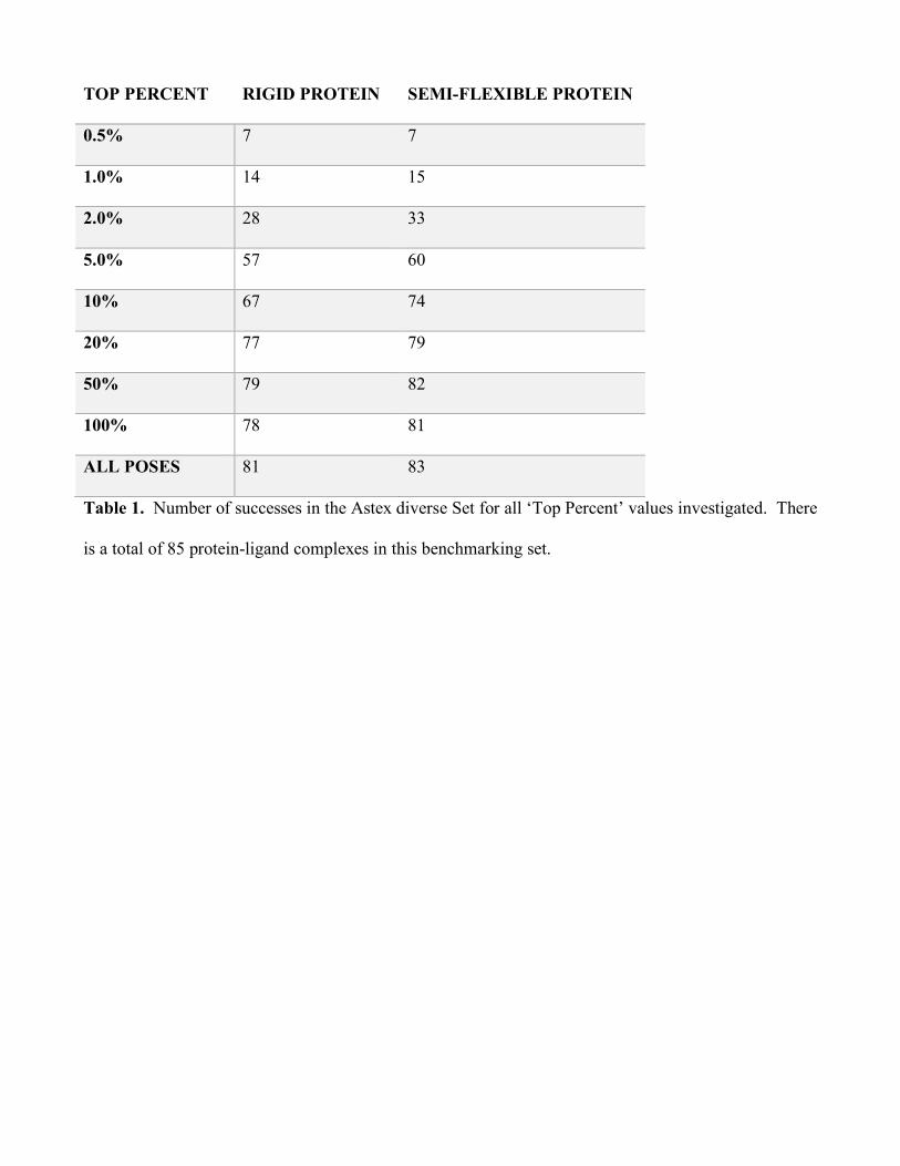
TOP PERCENT RIGID PROTEIN SEMI-FLEXIBLE PROTEIN

0.5% 7 7

1.0% 14 15

2.0% 28 33

5.0% 57 60

10% 67 74

20% 77 79

50% 79 82

100% 78 81

ALL POSES 81 83

Table 1. Number of successes in the Astex diverse Set for all ‘Top Percent’ values investigated. There

is a total of 85 protein-ligand complexes in this benchmarking set.

References

(1) Warren, G. L.; Andrews, C. W.; Capelli, A. M.; Clarke, B.; LaLonde, J.; Lambert, M. H.; Lindvall, M.; Nevins, N.; Semus, S. F.; Senger, S.; et al. A Critical Assessment of Docking Programs and Scoring Functions. J. Med. Chem. 2006, 49 (20), 5912–5931.

(2) Kellenberger, E.; Rodrigo, J.; Muller, P.; Rognan, D. Comparative Evaluation of Eight Docking Tools for Docking and Virtual Screening Accuracy. Proteins Struct. Funct. Bioinforma. 2004, 57 (2), 225–242.

(3) Bissantz, C.; Bernard, P.; Hibert, M.; Rognan, D. Protein-Based Virtual Screening of Chemical Databases. II. Are Homology Models of g-Protein Coupled Receptors Suitable Targets? Proteins Struct. Funct. Bioinforma. 2002, 50 (1), 5–25.

(4) Niu Huang; Brian K. Shoichet, * and; Irwin*, J. J. Benchmarking Sets for Molecular Docking. 2006.

(5) Wang, Z.; Sun, H.; Yao, X.; Li, D.; Xu, L.; Li, Y.; Tian, S.; Hou, T. Comprehensive Evaluation of Ten Docking Programs on a Diverse Set of Protein-Ligand Complexes: The Prediction Accuracy of Sampling Power and Scoring Power. Phys. Chem. Chem. Phys. 2016, 18, 12964–12975.

(6) Claußen, H.; Buning, C.; Rarey, M.; Lengauer, T. FLEXE: Efficient Molecular Docking Considering Protein Structure Variations. J. Mol. Biol. 2001, 308 (2), 377–395.

(7) Leach, A. R. Ligand Docking to Proteins with Discrete Side-Chain Flexibility. J. Mol. Biol. 1994, 235 (1), 345–356.

(8) Ding, F.; Yin, S.; Dokholyan, N. V. Rapid Flexible Docking Using a Stochastic Rotamer Library of Ligands. J. Chem. Inf. Model. 2010, 50 (9), 1623–1632.

(9) Apostolakis, J.; Plückthun, A.; Caflisch, A. Docking Small Ligands in Flexible Binding Sites. J. Comput. Chem. 1998, 19 (1), 21–37.

(10) Trott, O.; Olson, A. J. AutoDock Vina: Improving the Speed and Accuracy of Docking with a New Scoring Function, Efficient Optimization, and Multithreading. J. Comput. Chem. 2010, 31 (2), 455–461.

(11) Meng, E. C.; Gschwend, D. A.; Blaney, J. M.; Kuntz, I. D. Orientational Sampling and Rigid-Body Minimization in Molecular Docking. Proteins Struct. Funct. Genet. 1993, 17 (3), 266–278.

(12) Zhao, H.; Caflisch, A. Discovery of ZAP70 Inhibitors by High-Throughput Docking into a Conformation of Its Kinase Domain Generated by Molecular Dynamics. Bioorg. Med. Chem. Lett. 2013, 23 (20), 5721–5726.

(13) Zavodszky, M. I.; Kuhn, L. A. Side-Chain Flexibility in Protein-Ligand Binding: The Minimal Rotation Hypothesis. Protein Sci. 2005, 14 (4), 1104–1114.

(14) Chen, Y. C. Beware of Docking! Trends Pharmacol. Sci. 2015, 36 (2), 78–95. (15) Ruiz-Carmona, S.; Alvarez-Garcia, D.; Foloppe, N.; Garmendia-Doval, A. B.; Juhos, S.;

Schmidtke, P.; Barril, X.; Hubbard, R. E.; Morley, S. D. RDock: A Fast, Versatile and Open Source Program for Docking Ligands to Proteins and Nucleic Acids. PLoS Comput. Biol. 2014, 10 (4).

(16) Gaudreault, F.; Najmanovich, R. J. FlexAID: Revisiting Docking on Non-Native-Complex Structures. J. Chem. Inf. Model. 2015, 55 (7), 1323–1336.

(17) Nedumpully-Govindan, P.; Jemec, D. B.; Ding, F. CSAR Benchmark of Flexible MedusaDock in Affinity Prediction and Nativelike Binding Pose Selection. J. Chem. Inf. Model. 2016, 56 (6), 1042–1052.

(18) Verdonk, M. L.; Cole, J. C.; Hartshorn, M. J.; Murray, C. W.; Taylor, R. D. Improved Protein-Ligand Docking Using GOLD. Proteins Struct. Funct. Bioinforma. 2003, 52 (4), 609–623.

(19) Carlson, H. A.; Smith, R. D.; Damm-Ganamet, K. L.; Stuckey, J. A.; Ahmed, A.; Convery, M.

A.; Somers, D. O.; Kranz, M.; Elkins, P. A.; Cui, G.; et al. CSAR 2014: A Benchmark Exercise Using Unpublished Data from Pharma. J. Chem. Inf. Model. 2016, 56 (6), 1063–1077.

(20) Onodera, K.; Satou, K.; Hirota, H. Evaluations of Molecular Docking Programs for Virtual Screening. J. Chem. Inf. Model. 2007, 47 (4), 1609–1618.

(21) Feher, M.; Williams, C. I. Effect of Input Differences on the Results of Docking Calculations. J. Chem. Inf. Model. 2009, 49 (7), 1704–1714.

(22) Pevzner, Y.; Frugier, E.; Schalk, V.; Caflisch, A.; Woodcock, H. L. Fragment-Based Docking: Development of the CHARMMing Web User Interface as a Platform for Computer-Aided Drug Design. J. Chem. Inf. Model. 2014, 54 (9), 2612–2620.

(23) Belew, R. K.; Forli, S.; Goodsell, D. S.; O’Donnell, T. J.; Olson, A. J. Fragment-Based Analysis of Ligand Dockings Improves Classification of Actives. J. Chem. Inf. Model. 2016, 56 (8), 1597–1607.

(24) Vilar, S.; Cozza, G.; Moro, S. Medicinal Chemistry and the Molecular Operating Environment (MOE): Application of QSAR and Molecular Docking to Drug Discovery. Curr. Top. Med. Chem. 2008, 8 (18), 1555–1572.

(25) Freire, I. L. and E. Structural Stability of Binding Sites: Consequences for Binding Affinity and Allosteric Effects. Proteins Struct. Funct. Genet. 2000, 4, 63–71.

(26) Bernard, B.; Samudrala, R. A Generalized Knowledge-Based Discriminatory Function for Biomolecular Interactions. Proteins Struct. Funct. Bioinforma. 2009.

(27) Meng, E. C.; Lewis, R. A. Determination of Molecular Topology and Atomic Hybridization States from Heavy Atom Coordinates. J. Comput. Chem. 1991, 12 (7), 891–898.

(28) Wang, J.; Wolf, R. M.; Caldwell, J. W.; Kollman, P. A.; Case, D. A. Development and Testing of a General Amber Force Field. J. Comput. Chem. 2004, 25 (9), 1157–1174.

(29) Wang, J.; Wang, W.; Kollman, P. A.; Case, D. A. Automatic Atom Type and Bond Type Perception in Molecular Mechanical Calculations. J. Mol. Graph. Model. 2006, 25 (2), 247–260.

(30) Eastman, P.; Swails, J.; Chodera, J. D.; McGibbon, R. T.; Zhao, Y.; Beauchamp, K. A.; Wang, L.-P.; Simmonett, A. C.; Harrigan, M. P.; Stern, C. D.; et al. OpenMM 7: Rapid Development of High Performance Algorithms for Molecular Dynamics. PLOS Comput. Biol. 2017, 13 (7), e1005659.

(31) Allen, W. J.; Balius, T. E.; Mukherjee, S.; Brozell, S. R.; Moustakas, D. T.; Lang, P. T.; Case, D. A.; Kuntz, I. D.; Rizzo, R. C. DOCK 6: Impact of New Features and Current Docking Performance. J. Comput. Chem. 2015, 36 (15), 1132–1156.

(32) Groom, C. R.; Bruno, I. J.; Lightfoot, M. P.; Ward, S. C.; IUCr. The Cambridge Structural Database. Acta Crystallogr. Sect. B Struct. Sci. Cryst. Eng. Mater. 2016, 72 (2), 171–179.

(33) Rose, P. W.; Prlić, A.; Bi, C.; Bluhm, W. F.; Christie, C. H.; Dutta, S.; Green, R. K.; Goodsell, D. S.; Westbrook, J. D.; Woo, J.; et al. The RCSB Protein Data Bank: Views of Structural Biology for Basic and Applied Research and Education. Nucleic Acids Res. 2015, 43 (D1), D345–D356.

(34) Konc, J.; Janežič, D. An Improved Branch and Bound Algorithm for the Maximum Clique Problem. MATCH Commun. Math. Comput. Chem. MATCH Commun. Math. Comput. Chem 2007, 58, 569–590.

(35) Liu, D. C.; Nocedal, J. On the Limited Memory BFGS Method for Large Scale Optimization. Math. Program. 1989, 45 (1–3), 503–528.

(36) Liu, Z.; Su, M.; Han, L.; Liu, J.; Yang, Q.; Li, Y.; Wang, R. Forging the Basis for Developing Protein-Ligand Interaction Scoring Functions. Acc. Chem. Res. 2017, 50 (2), 302–309.

(37) Hartshorn, M. J.; Verdonk, M. L.; Chessari, G.; Brewerton, S. C.; Mooij, W. T. M.; Mortenson, P. N.; Murray, C. W. Diverse, High-Quality Test Set for the Validation of Protein-Ligand Docking Performance. J. Med. Chem. 2007.

(38) Nivedha, A. K.; Thieker, D. F.; Makeneni, S.; Hu, H.; Woods, R. J. Vina-Carb: Improving

Glycosidic Angles during Carbohydrate Docking. J. Chem. Theory Comput. 2016, 12 (2), 892–901.

(39) Bezhentsev, V. M.; Tarasova, O. A.; Dmitriev, A. V; Rudik, A. V; Lagunin, A. A.; Filimonov, D. A.; Poroikov, V. V. Computer-Aided Prediction of Xenobiotic Metabolism in the Human Body. Russ. Chem. Rev. 2016, 85 (8), 854–879.

(40) Kirchmair, J.; Göller, A. H.; Lang, D.; Kunze, J.; Testa, B.; Wilson, I. D.; Glen, R. C.; Schneider, G. Predicting Drug Metabolism: Experiment and/or Computation? Nature Reviews Drug Discovery. 2015.

(41) Kirchmair, J.; Williamson, M. J.; Tyzack, J. D.; Tan, L.; Bond, P. J.; Bender, A.; Glen, R. C. Computational Prediction of Metabolism: Sites, Products, SAR, P450 Enzyme Dynamics, and Mechanisms. Journal of Chemical Information and Modeling. 2012.

(42) Card, G. L.; England, B. P.; Suzuki, Y.; Fong, D.; Powell, B.; Lee, B.; Luu, C.; Tabrizizad, M.; Gillette, S.; Ibrahim, P. N.; et al. Structural Basis for the Activity of Drugs That Inhibit Phosphodiesterases. Structure 2004, 12 (12), 2233–2247.

(43) Cross, S. S. J. Improved FlexX Docking Using FlexS-Determined Base Fragment Placement. J. Chem. Inf. Model. 2005, 45 (4), 993–1001.

(44) Mysinger, M. M.; Carchia, M.; Irwin, J. J.; Shoichet, B. K. Directory of Useful Decoys, Enhanced (DUD-E): Better Ligands and Decoys for Better Benchmarking. J. Med. Chem. 2012, 55 (14), 6582–6594.

download fileview on ChemRxiv2018_Fine-Konc_candock.pdf (3.83 MiB)

Supporting information

CANDOCK: Chemical atomic network based hierarchical flexible docking algorithm using generalized statistical potentials

Jonathan Fine1, ‡, Janez Konc2, ‡, Ram Samudrala3, Gaurav Chopra1,4,5,6,7 *

1Department of Chemistry, Purdue University, 720 Clinic Drive, West Lafayette, IN 47906 2National Institute of Chemistry, Hajdrihova 19, SI−1000, Ljubljana, Slovenia 3Department of Biomedical Informatics, SUNY, Buffalo, NY, USA 4Purdue Institute for Drug Discovery 5Purdue Center for Cancer Research 6Purdue Institute for Inflammation, Immunology and Infectious Disease 7Purdue Institute for Integrative Neuroscience

‡These authors share equal contribution to this work.

*Corresponding Author E-mail: gchopra@purdue.edu

Figure S1: Distribution of RMSD values for all ligand poses generated by CANDOCK for the PDBbind Core set for (a) rigid-protein docking, (b) semi-flexible protein, and (c) fully-flexible protein docking.

Figure S2: Median number of poses generated for ligands containing 1-13 fragments divided by the top percent parameter.

Figure S3: Correlations between the RMR6 scores of the crystal poses and the pose with the lowest RMSD are shown for all eight top percent values for complexes in the PDBbind Core set. Poses within 2.0 Å of the crystal pose are shown in blue (successful runs) while poses greater than 2.0 Å (failures) are shown in red. For top percent values greater than 20%, the complexes that failed cluster above the y=x line. Therefore, in these cases, the CANDOCK algorithm did not sample the conformation space close to the binding pocket.

Figure S4: The lowest RMR6 score obtained for each cocrystal is plotted against the RMC15 score of the crystal pose. Poses within 2.0 Å of the crystal pose are shown in blue (successful runs) while poses greater than 2.0 Å are shown in red. The majority of points on this graph cluster below the y=x line, indicating that the RMR6 scoring function incorrectly scores several poses more favorably than the crystal pose, regardless of if the pose is close to the crystal pose. Therefore, there are potential improvements to be made for this scoring function.

Figure S5: Plots of the RMR6 score of all poses produced by CANDOCK for selected proteins in the PDBbind Core Set versus the RMSD of the pose. In all plots, the RMSD ranges from 1Å to 15Å. The poses were obtained using the semi flexible method at a ‘Top Percent’ value equal to 20%. These of these plots show a tunnel like affect around as one approaches an RMSD of zero, showing the scoring functions ability to select the crystal pose in these cases.

-100

-80

-60

-40

0 2 5 10 15

-40

-35

-30

-25

0 2 5 10 15

-60

-50

-40

-30

0 2 5 10 15

-50

-40

-30

0 2 5 10 15

-40

-36

-32

-28

0 2 5 10 15

-20

-15

-10

0 2 5 10 15

-60

-55

-50

-45

0 2 5 10 15-40

-30

-20

-10

0 2 5 10 15

1EBY 1MQ6

2XII 3EHY

3MSS 3RYJ

4CRA 4MGD

RMSD from crystal pose (A)

Sem

i-flex

ible

RMR6

sco

re (a

rbitra

ry u

nits)

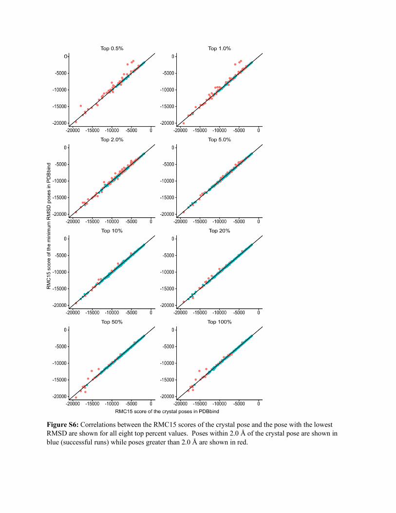
Figure S6: Correlations between the RMC15 scores of the crystal pose and the pose with the lowest RMSD are shown for all eight top percent values. Poses within 2.0 Å of the crystal pose are shown in blue (successful runs) while poses greater than 2.0 Å are shown in red.

Figure S7: The RMC15 score for the pose selected by RMR6 obtained for each cocrystal is plotted against the RMC15 score of the crystal pose. Poses within 2.0 Å of the crystal pose are shown in blue (successful runs) while poses greater than 2.0 Å are shown in red. Here it is shown that the successful poses occur only on the y=x line, while the unsuccessful poses cluster above this line. This indicates that further minization with RMC15 may improve the RMR6 selection rate.

Figure S8: Plots of the RMC15 score of all poses produced by CANDOCK for selected proteins in the PDBbind Core Set versus the RMSD of the pose. In all plots, the RMSD ranges from 1Å to 15Å The poses were obtained using the semi flexible method at a ‘Top Percent’ value equal to 20%. The trend seen for these proteins is as one decreases the RMC15 score, the RMSD of the predicted ligand also decreases. Therefore, the use of an objective function derived from the RMC15 scoring function to minimize the ligand in the binding pocket is justified.

-16000

-14000

-12000

-10000

0 5 10 15-2400

-2200

-2000

-1800

0 5 10 15

-3900

-3600

-3300

-3000

-2700

0 5 10 15

-8000

-7000

-6000

-5000

-4000

0 5 10 15

-3900

-3600

-3300

-3000

0 5 10 15

-8000

-7000

-6000

0 5 10 15

-5000

-4500

-4000

-3500

0 5 10 15

-2000

-1800

-1600

0 5 10 15

1EBY 1UTO

2HB1 2WBG

3FCG 3GE7

3QQS 3TWP

RMSD from crystal pose (A)

Sem

i-flex

ible

RMC1

5 sc

ore

(arb

itrary

unit

s) a

t 20%

Figure S9: Examples where CANDOCK is able to produce a good docking pose where other methods are not able. The best CANDOCK pose is given on the lefthand side of the figure and important interactions between the ligand protein are given on the right.

Rigid protein Semi-flexible protein Fully-flexible protein Average Median Average Median Average Median rmr4 0.095 0.049 0.095 0.049 0.140 0.080 rmr5 0.145 0.102 0.145 0.102 0.180 0.113 rmr6 0.176 0.115 0.176 0.115 0.189 0.130 rmr7 0.178 0.112 0.178 0.112 0.207 0.139 rmr8 0.190 0.112 0.190 0.112 0.212 0.165 rmr9 0.189 0.123 0.189 0.123 0.214 0.182 rmr10 0.203 0.141 0.203 0.141 0.236 0.212 rmr11 0.216 0.149 0.216 0.149 0.253 0.230 rmr12 0.225 0.165 0.225 0.165 0.262 0.246 rmr13 0.222 0.181 0.222 0.181 0.261 0.256 rmr14 0.210 0.169 0.210 0.169 0.249 0.236 rmr15 0.183 0.121 0.183 0.121 0.217 0.196 rmc4 0.307 0.279 0.307 0.279 0.361 0.360 rmc5 0.413 0.416 0.413 0.416 0.424 0.426 rmc6 0.459 0.473 0.459 0.473 0.462 0.471 rmc7 0.476 0.501 0.476 0.501 0.495 0.498 rmc8 0.498 0.519 0.498 0.519 0.518 0.528 rmc9 0.523 0.542 0.523 0.542 0.538 0.555 rmc10 0.537 0.560 0.537 0.560 0.550 0.559 rmc11 0.539 0.562 0.539 0.562 0.554 0.565 rmc12 0.546 0.571 0.546 0.571 0.561 0.579 rmc13 0.546 0.576 0.546 0.576 0.562 0.584 rmc14 0.556 0.587 0.556 0.587 0.560 0.587 rmc15 0.559 0.581 0.559 0.581 0.559 0.587 fmr4 0.081 0.027 0.081 0.027 0.121 0.071 fmr5 0.107 0.063 0.107 0.063 0.144 0.094 fmr6 0.125 0.064 0.125 0.064 0.155 0.106 fmr7 0.132 0.069 0.132 0.069 0.166 0.108 fmr8 0.152 0.079 0.152 0.079 0.177 0.102 fmr9 0.149 0.078 0.149 0.078 0.183 0.112 fmr10 0.149 0.070 0.149 0.070 0.183 0.114 fmr11 0.146 0.075 0.146 0.075 0.179 0.119 fmr12 0.135 0.062 0.135 0.062 0.164 0.114 fmr13 0.116 0.048 0.116 0.048 0.140 0.084 fmr14 0.093 0.023 0.093 0.023 0.110 0.053 fmr15 0.062 -0.014 0.062 -0.014 0.071 0.009 fmc4 0.307 0.270 0.307 0.270 0.360 0.353 fmc5 0.424 0.427 0.424 0.427 0.429 0.430 fmc6 0.468 0.480 0.468 0.480 0.468 0.480

fmc7 0.486 0.510 0.486 0.510 0.501 0.509 fmc8 0.505 0.527 0.505 0.527 0.523 0.530 fmc9 0.535 0.549 0.535 0.549 0.541 0.563 fmc10 0.539 0.560 0.539 0.560 0.552 0.563 fmc11 0.539 0.562 0.539 0.562 0.554 0.570 fmc12 0.545 0.569 0.545 0.569 0.561 0.581 fmc13 0.546 0.580 0.546 0.580 0.562 0.583 fmc14 0.556 0.587 0.556 0.587 0.558 0.586 fmc15 0.559 0.582 0.559 0.582 0.557 0.583 rcr4 0.050 -0.015 0.050 -0.015 0.115 0.053 rcr5 0.053 -0.015 0.053 -0.015 0.103 0.043 rcr6 0.056 -0.016 0.056 -0.016 0.096 0.036 rcr7 0.047 -0.018 0.047 -0.018 0.084 0.025 rcr8 0.057 -0.010 0.057 -0.010 0.090 0.022 rcr9 0.053 -0.013 0.053 -0.013 0.085 0.033 rcr10 0.039 -0.025 0.039 -0.025 0.066 0.007 rcr11 0.031 -0.035 0.031 -0.035 0.055 0.010 rcr12 0.031 -0.034 0.031 -0.034 0.054 0.007 rcr13 0.038 -0.031 0.038 -0.031 0.064 0.024 rcr14 0.057 -0.017 0.057 -0.017 0.089 0.037 rcr15 0.081 -0.006 0.081 -0.006 0.120 0.069 rcc4 0.067 0.001 0.067 0.001 0.119 0.047 rcc5 0.075 0.007 0.075 0.007 0.112 0.047 rcc6 0.073 0.013 0.073 0.013 0.099 0.040 rcc7 0.056 -0.005 0.056 -0.005 0.078 0.021 rcc8 0.051 -0.012 0.051 -0.012 0.067 0.000 rcc9 0.036 -0.028 0.036 -0.028 0.048 -0.010 rcc10 0.020 -0.053 0.020 -0.053 0.024 -0.028 rcc11 0.011 -0.073 0.011 -0.073 0.013 -0.043 rcc12 0.013 -0.072 0.013 -0.072 0.013 -0.043 rcc13 0.021 -0.061 0.021 -0.061 0.025 -0.030 rcc14 0.040 -0.044 0.040 -0.044 0.049 -0.009 rcc15 0.065 -0.010 0.065 -0.010 0.081 0.020 fcr4 0.050 -0.015 0.050 -0.015 0.115 0.062 fcr5 0.062 -0.002 0.062 -0.002 0.113 0.060 fcr6 0.071 -0.001 0.071 -0.001 0.117 0.056 fcr7 0.074 0.003 0.074 0.003 0.122 0.057 fcr8 0.084 0.014 0.084 0.014 0.130 0.070 fcr9 0.086 0.007 0.086 0.007 0.132 0.073 fcr10 0.091 0.011 0.091 0.011 0.138 0.072 fcr11 0.102 0.033 0.102 0.033 0.154 0.106

fcr12 0.116 0.047 0.116 0.047 0.171 0.115 fcr13 0.133 0.063 0.133 0.063 0.193 0.144 fcr14 0.157 0.091 0.157 0.091 0.221 0.181 fcr15 0.177 0.116 0.177 0.116 0.244 0.209 fcc4 0.063 -0.006 0.063 -0.006 0.112 0.054 fcc5 0.075 0.002 0.075 0.002 0.111 0.055 fcc6 0.084 0.019 0.084 0.019 0.116 0.057 fcc7 0.088 0.026 0.088 0.026 0.122 0.059 fcc8 0.098 0.021 0.098 0.021 0.131 0.064 fcc9 0.101 0.029 0.101 0.029 0.134 0.070 fcc10 0.105 0.036 0.105 0.036 0.141 0.076 fcc11 0.117 0.053 0.117 0.053 0.157 0.100 fcc12 0.132 0.071 0.132 0.071 0.175 0.121 fcc13 0.146 0.086 0.146 0.086 0.193 0.138 fcc14 0.163 0.107 0.163 0.107 0.215 0.165 fcc15 0.179 0.126 0.179 0.126 0.233 0.192

Table S1: Correlations between score and small molecule RMSD calculated and summarized over the entire PDBbind Core benchmarking set.

Selector: RMSD RMR6 RMC15 Ranker RMR6 RMC15 RMR6 RMC15 RMR6 RMC15

3-DEHYDROQUINATE DEHYDRATASE -0.716 -0.876 -0.852 -0.875 0.591 -0.874

ACETYLCHOLINE RECEPTOR 0.335 0.339 0.476 0.350 0.772 0.326

ACETYLCHOLINE-BINDING PROTEIN 0.482 -0.193 -0.004 -0.195 0.554 -0.212

ACHE -0.269 -0.664 -0.474 -0.688 -0.300 -0.652

ALPHA-L-FUCOSIDASE -0.692 -0.372 -0.606 -0.307 -0.666 -0.304

ALPHA-MANNOSIDASE II -0.271 -0.581 0.575 -0.580 0.855 -0.599

ANDROGEN RECEPTOR -0.919 0.734 -0.738 0.730 -0.776 0.736

TrpD 0.652 -0.905 -0.328 -0.832 0.539 -0.920

BETA-GLUCOSIDASE A 0.751 0.140 -0.337 0.119 -0.953 0.147

BETA-LACTAMASE -0.495 -0.894 -0.681 -0.908 0.835 -0.886

BETA-LACTOGLOBULIN -0.981 -0.991 -0.978 -0.997 -0.959 -0.993

BETA-SECRETASE 1 0.695 -0.116 -0.210 -0.370 0.673 -0.121

BROMODOMAIN-CONTAINING PROTEIN 4 -0.644 -0.981 -0.579 -0.988 0.393 -0.955

CAMP-DEPENDENT PROTEIN KINASE 0.696 -0.905 -0.619 -0.996 0.785 -0.864

CARBONIC ANHYDRASE 2 -0.694 -0.883 0.770 -0.770 0.976 -0.856

CATECHOL O-METHYLTRANSFERASE -0.858 -0.870 -0.749 -0.839 -0.687 -0.781

CELL DIVISION PROTEIN KINASE 2 -0.800 -0.899 0.713 -0.918 0.969 -0.879

CELLULAR TUMOR ANTIGEN P53 -0.739 -0.719 0.796 -0.719 0.925 -0.648

CGMP 3',5'-CYCLIC PHOSPHODIESTERASE -0.649 0.052 -0.138 0.103 -0.711 0.074

CHITINASE A -0.915 -0.725 -0.833 -0.725 -0.704 -0.682

COAGULATION FACTOR XA -0.963 -0.753 -0.992 -0.671 0.560 -0.596

FACTOR XI -0.805 -0.916 -0.864 -0.885 0.989 -0.887

DEHYDROSQUALENE SYNTHASE -0.353 -0.439 -0.727 -0.468 0.173 -0.432

ENDOTHIAPEPSIN -0.975 -0.993 -0.903 -0.992 0.971 -0.989

ESTROGEN RECEPTOR -0.843 0.764 0.501 0.764 -0.293 0.761

GLUTAMATE RECEPTOR 2 -0.814 -0.457 -0.741 -0.458 -0.854 -0.454

GLUTAMATE RECEPTOR, IONOTROPIC KAINATE 1

-0.977 -0.646 -0.702 -0.632 0.872 -0.577

GLYCOGEN PHOSPHORYLASE 0.716 0.383 -0.186 0.407 -0.833 0.341

HEAT SHOCK PROTEIN HSP82 -0.418 0.112 -0.574 0.105 -0.771 0.166

HEAT SHOCK PROTEIN HSP90-ALPHA -0.728 -0.879 -0.832 -0.882 0.778 -0.873

HIV-1 INTEGRASE -0.843 -0.954 -0.954 -0.960 0.935 -0.952

HIV-1 PROTEASE -0.916 -0.573 -0.907 -0.468 -0.926 -0.541

(MMP-1) -0.680 -0.815 -0.801 -0.808 0.966 -0.796

MITOGEN-ACTIVATED PROTEIN KINASE 14 -0.680 -0.902 -0.691 -0.903 0.916 -0.900

MTA/SAH NUCLEOSIDASE 0.601 0.203 0.601 0.203 0.657 0.206

O-GLCNACASE BT_4395 -0.974 -0.128 -0.471 -0.129 -0.392 -0.074

PANTOTHENATE SYNTHETASE -0.873 -0.960 -0.764 -0.961 0.835 -0.962

PPARG -0.974 -0.992 -0.971 -0.989 0.902 -0.983

PROTEIN-TYROSINE PHOSPHATASE 1B 0.304 -0.947 -0.080 -0.805 0.759 -0.874

QUEUINE TRNA-RIBOSYLTRANSFERASE -0.875 -0.697 -0.875 -0.697 -0.676 -0.703

RIBONUCLEASE A -0.701 -0.842 -0.908 -0.849 0.708 -0.836

RNA-DIRECTED RNA POLYMERASE -0.794 -0.831 -0.740 -0.828 0.981 -0.856

SERINE/THREONINE-PROTEIN KINASE 6 -0.093 -0.706 0.091 -0.885 -0.603 -0.619

CHK1 0.509 0.545 -0.204 0.637 0.963 0.386

PIM-1 0.656 0.447 0.423 0.436 -0.568 0.424

TANKYRASE-2 -0.918 -0.854 -0.970 -0.881 0.491 -0.825

THERMOLYSIN -0.610 0.178 -0.546 -0.272 -0.700 0.149

THROMBIN -0.798 0.154 0.473 0.188 0.562 0.155

TRANSCRIPTION ELONGATION FACTOR B POLYPEPTIDE 2

0.789 -0.772 0.784 -0.756 0.908 -0.770

TRANSPORTER -0.376 0.497 -0.284 0.509 -0.352 0.510

TRYPSIN BETA -0.905 -0.805 -0.927 -0.804 0.653 -0.769

TYROSINE-PROTEIN KINASE ABL1 0.929 -0.119 0.187 0.093 0.847 -0.221

TYROSINE-PROTEIN KINASE ITK/TSK 0.879 0.749 0.183 0.747 -0.786 0.755

TYROSINE-PROTEIN KINASE JAK1 -0.552 -0.093 -0.292 -0.154 0.234 -0.079

TYROSINE-PROTEIN KINASE JAK2 -0.653 -0.883 -0.718 -0.876 0.759 -0.931

UROKINASE-TYPE PLASMINOGEN ACTIVATOR

-0.909 -0.927 -0.908 -0.922 0.882 -0.924

Table S2: Pearson correlations for all ligands in the PDBbind Core set using various scoring functions to select the representative pose for the protein-ligand complex and rank the activity of the ligand versus other ligands for the same protein. Highlighted values are plotted in Figure S7.

Selector RMSD RMR6 RMC15 Ranker RMR6 RMC15 RMR6 RMC15 RMR6 RMC15

3-DEHYDROQUINATE DEHYDRATASE -0.400 -0.600 -1.000 -0.600 0.700 -0.600

ACETYLCHOLINE RECEPTOR 0.400 0.100 0.600 0.100 0.600 0.100

ACETYLCHOLINE-BINDING PROTEIN 0.500 -0.300 -0.600 -0.300 0.700 -0.300

ACHE -0.500 -0.700 -0.400 -0.700 -0.300 -0.700

ALPHA-L-FUCOSIDASE -0.700 0.400 -0.700 0.400 -0.700 0.400

ALPHA-MANNOSIDASE II -0.300 -0.300 0.300 -0.300 0.700 -0.300

ANDROGEN RECEPTOR -0.700 0.900 -0.600 0.900 -1.000 0.900

TrpD 0.500 -1.000 -0.500 -0.900 0.300 -1.000

BETA-GLUCOSIDASE A 0.700 0.300 -0.400 0.300 -1.000 0.300

BETA-LACTAMASE -0.455 -0.782 -0.745 -0.879 0.758 -0.782

BETA-LACTOGLOBULIN -1.000 -1.000 -1.000 -1.000 -1.000 -1.000

BETA-SECRETASE 1 0.500 0.000 -0.300 -0.400 0.700 0.000

BROMODOMAIN-CONTAINING PROTEIN 4

-0.700 -0.900 -0.600 -1.000 0.200 -0.900

CAMP-DEPENDENT PROTEIN KINASE 0.700 -1.000 -0.400 -1.000 0.600 -1.000

CARBONIC ANHYDRASE 2 -0.600 -0.800 0.700 -0.800 0.900 -0.800

CATECHOL O-METHYLTRANSFERASE -0.800 -0.900 -0.700 -0.900 -0.900 -0.900

CELL DIVISION PROTEIN KINASE 2 -0.600 -0.700 0.500 -0.700 0.900 -0.700

CELLULAR TUMOR ANTIGEN P53 -0.900 -0.700 0.900 -0.700 0.900 -0.400

CGMP 3',5'-CYCLIC PHOSPHODIESTERASE

-0.700 0.000 -0.300 0.000 -0.700 0.000

CHITINASE A -0.900 -0.700 -0.900 -0.700 -0.800 -0.700

FACTOR XA -0.900 -0.900 -1.000 -0.900 0.700 -0.900

FACTOR XI -0.700 -0.600 -0.700 -0.300 0.900 -0.300

DEHYDROSQUALENE SYNTHASE -0.600 -0.100 -0.800 -0.200 0.500 -0.600

ENDOTHIAPEPSIN -1.000 -1.000 -0.900 -0.900 1.000 -0.900

ESTROGEN RECEPTOR -0.800 0.300 0.300 0.300 -0.600 0.300

GLUTAMATE RECEPTOR 2 -0.700 -0.700 -0.700 -0.700 -0.900 -0.700

GLUTAMATE RECEPTOR, IONOTROPIC KAINATE 1

-1.000 -0.700 -0.700 -0.700 0.900 -0.700

GLYCOGEN PHOSPHORYLASE 0.900 0.300 0.200 0.300 -0.800 0.300

HEAT SHOCK PROTEIN HSP82 -0.500 0.400 -0.600 0.400 -0.800 0.400

HEAT SHOCK PROTEIN HSP90-ALPHA -0.600 -0.800 -0.700 -0.800 0.900 -0.800

HIV-1 INTEGRASE -0.900 -1.000 -0.900 -1.000 0.700 -1.000

HIV-1 PROTEASE -0.900 -0.700 -0.900 -0.800 -1.000 -0.600

MMP-12 -0.900 -0.900 -0.900 -0.900 0.900 -0.900

MITOGEN-ACTIVATED PROTEIN KINASE 14

-0.700 -0.900 -0.700 -1.000 0.900 -0.900

MTA/SAH NUCLEOSIDASE 0.700 -0.100 0.700 -0.100 0.600 -0.100

O-GLCNACASE BT_4395 -0.900 -0.600 -0.500 -0.600 -0.600 -0.600

PANTOTHENATE SYNTHETASE -0.900 -1.000 -0.900 -1.000 0.800 -1.000

PPARG -0.700 -1.000 -1.000 -1.000 1.000 -1.000

PROTEIN-TYROSINE PHOSPHATASE 1B 0.400 -1.000 -0.300 -0.700 0.700 -0.900

QUEUINE TRNA-RIBOSYLTRANSFERASE -0.700 -0.600 -0.700 -0.600 -0.600 -0.600

RIBONUCLEASE A -0.700 -0.700 -0.900 -0.700 0.400 -0.700

RNA-DIRECTED RNA POLYMERASE -0.600 -1.000 -0.900 -1.000 1.000 -1.000

SERINE/THREONINE-PROTEIN KINASE 6 -0.500 -0.900 -0.500 -0.900 -0.600 -0.700

CHK1 0.600 0.600 -0.400 0.600 1.000 0.600

PIM-1 0.300 0.300 0.200 0.300 -0.300 0.300

TANKYRASE-2 -1.000 -0.800 -0.900 -0.900 0.500 -0.800

THERMOLYSIN -0.600 0.000 -0.600 -0.400 -0.400 0.000

THROMBIN -0.800 0.400 0.300 0.400 0.500 0.200

TCEB2 0.700 -0.700 0.800 -0.700 0.800 -0.700

TRANSPORTER -0.500 0.700 -0.300 0.700 -0.600 0.700

TRYPSIN BETA -0.900 -0.800 -0.900 -0.800 0.600 -0.800

TYROSINE-PROTEIN KINASE ABL1 1.000 -0.300 -0.400 -0.300 0.900 -0.300

TYROSINE-PROTEIN KINASE ITK/TSK 0.900 0.700 -0.100 0.700 -0.400 0.500

TYROSINE-PROTEIN KINASE JAK1 -0.600 -0.300 -0.600 -0.300 0.500 -0.300

TYROSINE-PROTEIN KINASE JAK2 -0.700 -0.900 -0.900 -0.900 0.700 -0.900

UROKINASE-TYPE PLASMINOGEN ACTIVATOR

-0.900 -0.900 -0.900 -0.900 1.000 -0.900

Table S3: Spearman correlations for all ligands in the PDBbind Core set using various scoring functions to select the representative pose for the protein-ligand complex and rank the activity of the ligand versus other ligands for the same protein. Highlighted values are plotted in Figure S7.

Figure S10: Rigid protein docking correlations between the RMC15 score and the measured pKd/pKi of the compounds in the PDBbind for each protein target. The representative docked ligand pose for ranking was selected with either the lowest RMSD or the best RMR6 score criterion.

Figure S11: Semi-flexible protein docking correlations between the RMC15 score and the measured pKd/pKi of the compounds in the PDBbind for each protein target. The representative docked ligand pose for ranking was selected with either the lowest RMSD or the best RMR6 score criterion.

Figure S12: Fully flexible protein docking correlations between the RMC15 score and the measured pKd/pKi of the compounds in the PDBbind for each protein target. The representative docked ligand pose for ranking was selected with either the lowest RMSD or the best RMR6 score criterion.

Figure S14: Plots of the ligand pKi/pKd against the best pose RMSD obtained using the semi-flexible method broken down by the ‘Top Percent’ parameter. These plots show there is no relationship between RMSD and pKi.

Figure S14: Plots of the ligand pKi/pKd against the RMR selected pose RMSD obtained using the semi-flexible method broken down by the ‘Top Percent’ parameter. These plots show there is no relationship between RMSD and pKi when the pose is selected by RMR6..

Figure S15: Interaction potentials for selected IDATM atom type pairs in the RMC15 objective function. These interactions are selected due to their conventionally repulsive/attractive/neutral nature, or due to their interest in drug discovery.

download fileview on ChemRxiv2018_Fine-Konc_candock_SI.pdf (3.89 MiB)