canadian hydraulic centre

8/7/2019 Canadian Hydraulic centre

http://slidepdf.com/reader/full/canadian-hydraulic-centre 1/40

Hydrodynamic model ofSt. Clair River

with Telemac-2D

Phase 2 report

Controlled Technical Report CHC-CTR-084 revision 1

March 2009



NRC-CHC has prepared this report for the International Joint Commission (IJC) basedon data supplied by IJC, its Commissioners, staff, consultants, or contractors. NRC-CHCdoes not guarantee the accuracy or validity of such data, and does not guarantee thatany software used in the work reported herein is free from errors not disclosed so far.

In preparing this report and making it available to IJC, NRC-CHC expressly is notundertaking to render professional services or provide advice to, or on behalf of, anythird party. Furthermore, NRC-CHC expressly is not undertaking to perform any dutyowed to any third person or entity by any other person or entity. NRC-CHC does notguarantee that the contents of this report meet the requirements of any third party. Theinformation in this report is directed exclusively to those with the appropriate degree oftraining and experience to use and apply its contents.

This report is provided without any representations, warranties, or conditions of any kind,express or implied, including, without limitation, implied warranties or conditions aboutthe document’s fitness for a particular purpose or use, its merchantability, or its non-

infringement of any third party’s intellectual property. However, NRC warrants that it hasnot knowingly infringed any other party’s intellectual property.

Note to revision 1

Since the publication of report CHC-CTR-084 in October 2008, additional studies wereperformed on the St Clair River using the CHC Telemac model.It was felt that these studies should be reported formally in the revision 1 of this reportwhich differs from the original version by the addition of:

• Section 5, lowering the bottom artificially• Section 8.5, change in recirculation zone

• Section 8.6, change in average sediment volume on the bottom

• Section 9, sensitivity to actual bathymetric survey location



Hydrodynamic model ofSt. Clair River

with Telemac-2D

Phase 2 report

Controlled Technical Report CHC-CTR-084 revision 1

March 2009

Canadian Hydraulics CentreNational Research Council

Ottawa, OntarioK1A 0R6

Prepared for: International Joint CommissionInternational Upper Great Lakes Study234 Laurier Avenue West, 22nd FloorOttawa, ONK1P 6K6



CHC-CTR-084 i

Table of Content

1. Introduction................................................................................................................1

2. Model Modification.....................................................................................................1

2.1 Turbulence model..............................................................................................1

2.2 Calibration with 2007 bathymetry ...................................................................... 8

3. Comparison with monthly average data ..................................................................11

4. Preparation of a new model based on 1971 data....................................................12

5. Effect of artificial change in bathymetry using the 1971 model ...............................16

6. Calibration with the modified 2007 bathymetric survey, and modified flows ...........16

7. Comparison 1971 - 2007 levels............................................................................... 17

7.1 Comparison 1971 - 2007 bottom friction .........................................................18

8. Further analysis on the 1971 - 2007 changes .........................................................19

8.1 Sensitivity of 1971 calibration ..........................................................................19

8.2 Sensitivity of bottom roughness.......................................................................19

8.3 Sensitivity on 2007 discharges used in calibration ..........................................20

8.4 Sensitivity on 2007 bathymetry representation................................................20

8.5 Change in recirculation zone downstream of Blue Water Bridge ....................20

8.6 Comparison 1971 - 2007 volume of bottom sediments ...................................24

9. Effect of changing the location of a bathymetric survey ..........................................24

10. Conclusion...........................................................................................................31

11. References ..........................................................................................................31



CHC-CTR-084 ii

List of Tables

Table 1 - Comparison between measured and simulated levels after 2007 calibration ..10

Table 2 - Steady-state simulated flows over a wider range.............................................11

Table 3 - Overall calibration of 1971 model..................................................................... 16

Table 4 - Impact of Bathymetry Changes on Lake Huron levels with the 1971 model....16

Table 5 - Comparison between measured and simulated levels after 2007 modified calibration................................................................................................................................17

Table 6 - Changes in levels along the river between 1971 and 2007 .............................18

Table 7 - Changes due to shift in Bathymetric survey.....................................................25

List of Figures

Figure 1 - Velocity vectors from 2003 survey (vertically averaged)...................................2

Figure 2 - Comparison: survey with K-epsilon model........................................................ 3

Figure 3 - Comparison: survey with Elder model ..............................................................3

Figure 4 - Comparison: survey with Smagorinsky model ..................................................4

Figure 5 - Cross-section location.......................................................................................5 Figure 6 - Cross-sectional velocity profile - Comparison for the upstream section before fluid starts to

turn ............................................................................................................................ 5

Figure 7 - Cross-sectional velocity profile comparison in the river bend...........................6

Figure 8 - Model Flows in various locations along St. Clair River during July 1-2, 2003 period 7

Figure 9 - Definition of the coarser bathymetric set of points, derived from the high density data 9

Figure 10 - Bathymetry data used in the upper portion .....................................................9

Figure 11 - Sensitivity of St. Clair River discharges to changes in Lake Huron levels .... 12

Figure 12 - Head difference measured during 1968 and 1973 flow surveys...................13

Figure 13 - Head difference measured during 1968 and 1973 flow surveys...................14

Figure 14 - St. Clair Shore levels during the 1968,1973 surveys ....................................15

Figure 15 - Changes in roughness coefficient between 1971 and 2007 .........................19

Figure 16 - Recirculation zone in first bend of St.Clair River..........................................21`

Figure 17 - Transverse section of water velocity profile (m/s), in sections 1 and 2.........22



CHC-CTR-084 iii

Figure 18 - Transverse section of water velocity profile (m/s), in sections 3 and 4.........23

Figure 19 - Stag Island shifted South..............................................................................26

Figure 20 - Stag Island shifted North...............................................................................27

Figure 21 - Bend upstream of Fawn Islands shifted South .............................................28

Figure 22 - Bend upstream of Fawn Islands shifted North ..............................................29

Figure 23 - Resulting typical cross sections, after shift ...................................................30



CHC-CTR-084 1

1. Introduction

As part of the International Upper Great Lakes Study, a two dimensional numerical model ofSt. Clair River was developed using Telemac software (ref 1).

This model was well calibrated with the multi-beam 2002 bathymetry survey in the upperportion of the River, the 2000 single-beam survey for its lower portion, and the existingstage-discharge relationships. It has a very fine grid mesh in the upper portion of the river(15 m) which allows the proper description of small bottom irregularities. It was usedextensively to simulate changes, such as bathymetry, morphology, and bed material contentor its bottom friction, which may have occurred in the last 35 years, and to assess theimpacts of these changes on the river hydrodynamics.

In order to improve the model range of applicability, the following modifications wereperformed:

o Check the model transect velocity profiles, with ADCP velocity measurements incross-sections downstream from Blue Water Bridge, in order to verify the sizeand strength of current recirculation.

o Recalibrate using the 2007 multi-beam bathymetric survey

The model was then used too Verify model range of applicability using monthly average data, in a wider range

of flows and levels.o

Re-calibrate the model with measurement data available from the 1971 era,(flow and levels).o Compare 1971/2007 river hydrodynamics using the two 1971 and 2007 models.o Assess sensitivity of the quality of the input data on the results

2. Model Modification

2.1 Turbulence model

In the numerical model, the velocity gradient across the river is defined by the turbulencealgorithm used. This turbulence will specify the local fluid viscosity or diffusivity to bestsimulate the velocity gradient.

In the original model, the K-Epsilon algorithm was chosen to simulate the turbulence in theflow. It is one of the standard algorithms in 2D numerical modeling.

In order to verify the model turbulence, the large recirculation in the bend of the St. ClairRiver downstream from the Blue Water Bridge was investigated in detail. ADCPmeasurements from July 2003 were used to compare model with measurements.



CHC-CTR-084 2

Several sets of ADCP were collected by the USGS and the US Army Corps of Engineers atthe same period of time (Reference 4).

The 3D measurements were reduced by Environment Canada, vertically averaged, andprocessed on a regular square grid at 1m intervals for the USACE data, and 5m for theUSGS. Figure 1 shows the vertically averaged velocity vectors, derived from their twohorizontal components, as measured on July 2, 2003 by the two organizations.

Figure 1 - Velocity vectors from 2003 survey (vertically averaged)

As a comparison, the Telemac model was run with thee different turbulence algorithms:K-epsilon, Elder, and Smagorinsky. They are shown in Figures 2 to 4 which indicate that theK-epsilon model provides a narrower recirculation zone whereas the other two modelsprovide a better representation of the flow pattern.



CHC-CTR-084 3

Figure 2 - Comparison: survey with K-epsilon model

Figure 3 - Comparison: survey with Elder model



CHC-CTR-084 4

Figure 4 - Comparison: survey with Smagorinsky model

The velocity profiles in several cross-sections of the river bend (shown in figure 5) wereprepared. Figure 6 shows that at section 1, where the flow in the river has not started toturn, the three turbulence algorithms give the same velocity profile. Further downstream,there is a strong three-dimensional component to the velocity vector and each turbulencealgorithm (all of which are two dimensional) reacts differently to non-2D hydrodynamics, asseen in Figure 7 for the sections 4 and 5.



CHC-CTR-084 5

Figure 5 - Cross-section location

Figure 6 - Cross-sectional velocity profile - Comparison for the upstream section before fluidstarts to turn



CHC-CTR-084 6

Figure 7 - Cross-sectional velocity profile comparison in the river bend



CHC-CTR-084 7

A few notes of explanation for the graphs in Figure 7:

• The apparent drop to zero velocity on the ADCP surveys on the edges of the sectionis due to the lack of data close to the shore.

• The difference between the two surveys may come from the interpolation process.The cross-sections are in a straight line whereas the surveys were collected along

meandering boat paths (fig 1). The curves shown in Figure 7 are an interpolationbetween several boat paths. This interpolation has not been performed along streamlines.

• The Elder and Smagorinsky models provide a better match to the overall cross-sectional profile than the K-epsilon model.

• In general the velocities from the model are smaller than the ADCP measurementsbecause the model was calibrated from existing flow-level relationships.

• A preliminary investigation has been performed on the flows obtained during thesesimulations. Figure 8 shows the instantaneous cross section flows as estimated bythe Telemac model when it was run with hourly levels prescribed at Lakeport and atSt. Clair Shores. In this figure the beginning of the plots corresponds to 30 June

2003, 18h00. (The model was started a week earlier to insure proper dynamic set-up).

Figure 8 - Model Flows in various locations along St. Clair River during July 1-2, 2003period



CHC-CTR-084 8

Figure 8 shows flows of the order of 4530 m3/s. These flows can be compared withmeasurements taken on July 1st 2003:

• the ADCP measurements of the order of 5000 m3/s,

• the Environment Canada estimates of the order of 4700 m3/s, based on stagerelationships

• the USACE estimates of the order of 4500 m3/s, based on stage relationships

This shows that this aspect of flow estimate needs more in-depth analysis, which was notpart of this study.

Following these investigations, it was decided to use the Elder turbulence algorithm infuture simulations, since it gives a better representation of the velocity profile, and it has a

better representation of dispersion.

2.2 Calibration with 2007 bathymetry

The original model was calibrated with the 2002 bathymetric data for the upper section ofthe St. Clair River, and the 2000 data for the lower section from downstream of the mouthof the Black River to Algonac.

Using the 2007 survey would provide a more accurate model which would better representthe actual morphology of the St. Clair River, since it was a multi-beam survey from FortGratiot to Algonac.

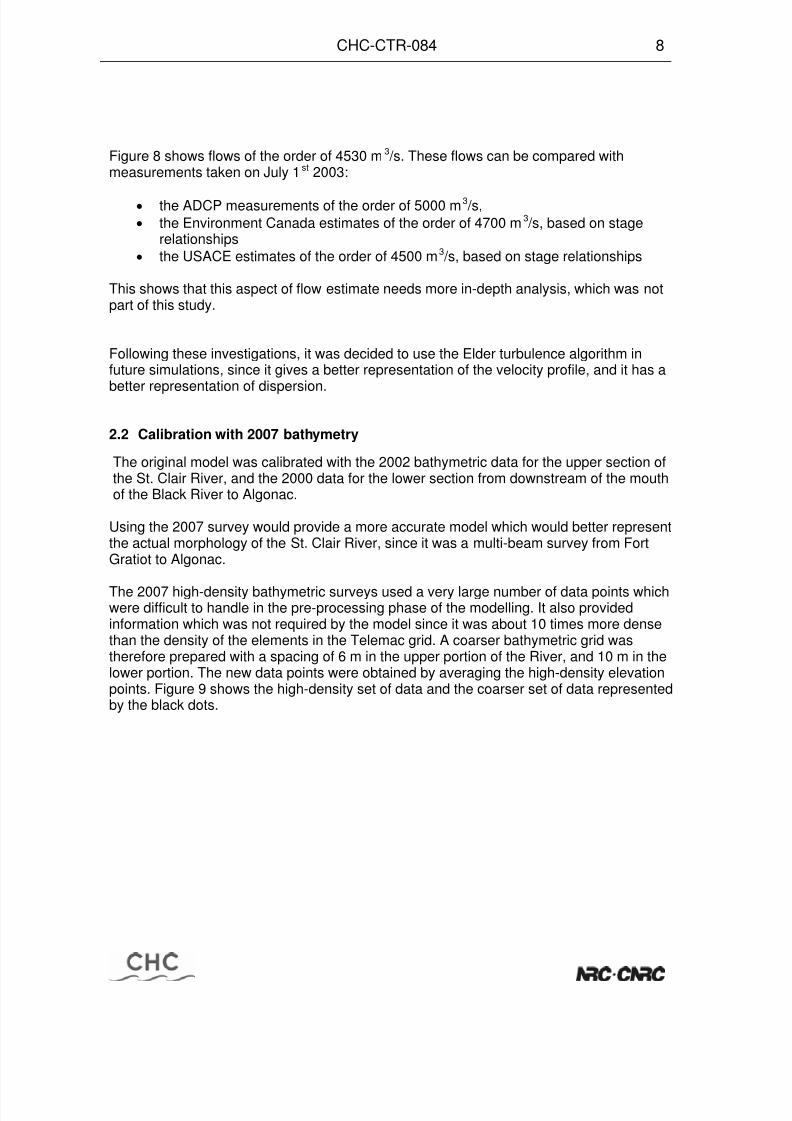
The 2007 high-density bathymetric surveys used a very large number of data points whichwere difficult to handle in the pre-processing phase of the modelling. It also providedinformation which was not required by the model since it was about 10 times more densethan the density of the elements in the Telemac grid. A coarser bathymetric grid wastherefore prepared with a spacing of 6 m in the upper portion of the River, and 10 m in thelower portion. The new data points were obtained by averaging the high-density elevationpoints. Figure 9 shows the high-density set of data and the coarser set of data representedby the black dots.



CHC-CTR-084 9

Figure 9 - Definition of the coarser bathymetric set of points, derived from the high densitydata

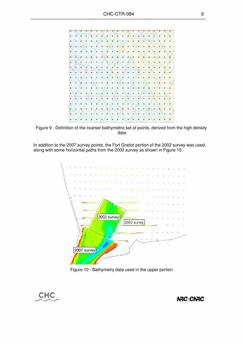
In addition to the 2007 survey points, the Fort Gratiot portion of the 2002 survey was used,along with some horizontal paths from the 2000 survey as shown in Figure 10.

Figure 10 - Bathymetry data used in the upper portion



CHC-CTR-084 10

The calibration/verification was done over the same three time periods as in the originalTelemac model, during which the levels and the flow could be considered steady for severaldays. This ensured that the flows were the same at the upstream and downstream ends of

the St. Clair River and at the exit of St. Clair Lake. (See ref 1). The flows were obtainedfrom the existing stage-discharge relationships provided by Environment Canada(Reference 5). Their derivation is explained in more detail in Ref. 1.

Table 1 shows the levels simulated by the model, as compared to the measured level at thevarious gauging stations. The maximum difference was 18 mm and the minimum was -17mm, both occurring at the Dunn Paper gauge. In this calibration the bottom frictioncoefficients for the estuary channels (lower St. Clair River) were maintained in the sameratio as found in the original calibration in order to keep the same flow distribution amongthe channels.

Calibration 2007 bathymetryEC existing relationships

Flow 4295 m3/s 5020 m

3/s 5660 m

3/s

run number 124 123 122

Year 2001 2002 1998

Days 90-96 194-199 170-176

measured simul diff measured simul diff measured simul diff

Lakeport (m) 175.770 175.771 0.001 176.35 176.335 -0.015 176.88 176.892 0.012

Fort Gratiot (m) 175.740 175.731 -0.009 176.28 176.29 0.010 176.83 176.844 0.014

Dunn Paper (m) 175.650 175.633 -0.017 176.18 176.171 -0.009 176.69 176.708 0.018

Point Edward (m) 175.580 175.581 0.001 176.11 176.099 -0.011 176.62 176.621 0.001

Mouth Of Black (m) 175.560 175.553 -0.007 176.09 176.076 -0.014 176.59 176.603 0.013

Dry Dock (m) 175.460 175.461 0.001 175.98 175.969 -0.011 176.48 176.489 0.009

St. Clair SP (m) 175.170 175.172 0.002 175.65 175.643 -0.007 176.14 176.145 0.005

Point Lambton (m) 174.880 174.88 0.000 175.30 175.302 0.002 175.78 175.775 -0.005

Algonac (m) 174.830 174.842 0.012 175.26 175.26 0.000 175.73 175.731 0.001

St. Clair Shores (m) 174.690 174.687 -0.003 175.10 175.097 -0.003 175.58 175.57 -0.010

Table 1 - Comparison between measured and simulated levels after 2007 calibration

The 2007 calibration roughness coefficients showed a slight increase. This increase couldbe due to a change in the bottom since 2000, but it is felt that this change is mainly due tothe change in the representation of the bottom in the numerical mesh. The 2007 data ismuch more dense, and therefore provides a smoother numerical representation in themodel which must be compensated for by higher friction factors.

It is to be noted that this calibration was performed using the Stage-fall-dischargerelationships from Environment Canada to obtain the flows during steady state periods, withflows at 4295, 5050 and 5660 m3/s.

Actual flow measurements have also been utilized to calibrate the model in a separatecalibration, by using the flows and levels from the RMA model calibration (Ref 2). Whentrying to calibrate, using scenarios 1, 7 and 4 (from Ref 2), with flows 4905, 5604 and 6302m3/s, levels at the same gauging stations showed errors from 3 to 13 cm, with an averageerror of 6 cm. For the 5604 m3/s “medium” flow, the average error was smaller, 4 cm, with amaximum error at Dunn Paper of 8 cm.



CHC-CTR-084 11

These errors are much higher than those indicated in Table 1. It is thought that this comesfrom the fact that the flows and levels in Ref 2 do not correspond to steady state, and thatweeds may have come into effect with the seasonal change of the roughness. Thiscalibration was therefore not retained.

3. Comparison with monthly average data

In order to assess the range of applicability of the new model, with the 2007 bathymetry, theflows from Table 2 were simulated in a steady state situation. These correspond to averagemonthly flows and levels as provided by Ref. 3. The average monthly levels were obtainedfrom NOAA, while Environment Canada calculated the flows using its level-gaugerelationships. It can be seen from Table 2 that for the higher flows, an error of the order of 7cm can be expected for the level at Fort Gratiot. As seen in figure 11, this would correspondto an error in flows of 175 m3/s or 2.6%.

AVERAGE MONTHLY DATA

level

SC

Shores

Q from

Huron

level Fort

Gratiot

observed

level Fort Gratiot

simulated difference

Year Month m m3/s m m m

1986 8 175.89 6630 177.34 177.41 0.07

1997 9 175.68 6280 177.09 177.15 0.06

1998 5 175.63 5800 176.86 176.94 0.08

1995 10 175.08 5310 176.38 176.40 0.02

2004 7 175.15 5080 176.34 176.35 0.01

2006 6 175.00 4750 176.11 176.12 0.01

2001 4 174.74 4340 175.79 175.79 0.00

Table 2 - Steady-state simulated flows over a wider range



CHC-CTR-084 12

Sensitivity of St. Clair River Discharge

to Lake Huron levels(5680 m

3/s - Huron:176.73 m - St. Clair:175.29 m)

-0.18

-0.16

-0.14

-0.12

-0.10

-0.08

-0.06

-0.04

-0.02

0.00

0.02

0.04

0.06

0.08

0.100.12

0.14

0.16

0.18

-400 -350 - 300 -250 - 200 -150 - 100 -50 0 50 100 150 200 250 300 350 400

Variation in Q (m3/s)

Variation in Huron surface elevation (m)

Figure 11 - Sensitivity of St. Clair River discharges to changes in Lake Huron levels

4. Preparation of a new model based on 1971 data.

In the previous study (ref 1), the Telemac model was run with the bathymetry as it wassurveyed in 1971, and a comparison with today’s data showed that Lake Huron levels woulddrop by 13 cm if nothing else changed between 1971 and 2007. This important finding wasbased on the assumption that the bottom roughness did not change during this period.

In order to verify this assumption, a Telemac model of the St. Clair River was preparedusing all information available from the 1971 era. Flows had been recorded in variouscross-sections in 1968 and 1973 using conventional survey methods.



CHC-CTR-084 13

Level difference Fort Gratiot - Dry Dock

0.1

0.2

0.3

0.4

0.5

0.6

4000 4500 5000 5500 6000 6500 7000

Measured Discharge (m3/s)

Level difference ( m)

Bay Point 1968 Robert Landing 1968

Dry Dock 1973 SC State 1973

Simulation

Level difference Dry Dock - SC state

0.1

0.2

0.3

0.4

0.5

0.6

4000 4500 5000 5500 6000 6500 7000





Simulation

Figure 12 - Head difference measured during 1968 and 1973 flow surveys



CHC-CTR-084 14

Level difference SC state - Algonac

0.1

0.2

0.3

0.4

0.5

0.6

4000 4500 5000 5500 6000 6500 7000





Simulation

Level difference Algonac - St Clair Shores

0

0.1

0.2

0.3

0.4

0.5

4000 4500 5000 5500 6000 6500 7000




Dry Dock 1973 FG Algonac

Simulation

Figure 13 - Head difference measured during 1968 and 1973 flow surveys



CHC-CTR-084 15

Figures 12 and 13 show the level differences between the various gauge stations for thecorresponding recorded flow. Figure 14 shows that the 1968 and 1973 surveys were madeat two different St. Clair lake levels.

In the preparation of these graphs, all surveys where the levels or flows were questionable

have not been used.

St Clair Shores levels

175

175.2

175.4

175.6

175.8

176

4000 4500 5000 5500 6000 6500 7000


Level ( m)



Simulation

Figure 14 - St. Clair Shore levels during the 1968,1973 surveys

In order to reproduce these conditions with the Telemac model, three scenariosrepresented by the three large square dots on Figures 12, 13, and 14 were assumed.

These would correspond to three “average” situations with discharges of 5000, 5750 and6500 m3/s.

The model was calibrated so as to minimize the errors in levels at four gauging stations forthese three discharges. The maximum errors were of the order of ±7 cm as shown in Table3.



CHC-CTR-084 16

CONDITION 1 CONDITION 2 CONDITION 3

5000 m3/s 5750 m3/s 6500 m3/s

Estimated simulated diff Estimated simulated diff Estimated simulated dif

Fort Gratiot 176.39 176.32 -0.07 176.53 176.61 0.08 177.23 177.29 0

Dry Dock 176.08 176.02 -0.06 176.17 176.24 0.07 176.86 176.88 0

St.Cl State Police 175.74 175.70 -0.04 175.80 175.84 0.04 176.45 176.49 0

Algonac 175.35 175.33 -0.02 175.35 175.37 0.02 176.00 176.01 0

St. Clair Shores 175.20 175.20 0.00 175.20 175.20 0.00 175.85 175.85 0

Table 3 - Overall calibration of 1971 model

It is to be noted that this error of 7 cm is of the same order of magnitude as the one foundwhen trying to calibrate the model with the RMA2 data (section 2.2). Both the RMA data andthe 1971 data are based on actual level and flow information averaged over many hours.

5. Effect of artificial change in bathymetry using the 1971 model

We recall that with the 2002 model, (ref 1, revision 1, Table 10), the lowering of thebathymetry along the river from Fort Gratiot to Algonac by 50 cm created a drop of LakeHuron level by 11.1 cm.

The same scenario was tested on the 1971 model (1971 bathymetry, calibrated using1968/1973 data as per Table 3). If the river bottom is lowered by 50 cm, Lake Huron leveldrops by 11.6 cm, as shown in Table 4. This is almost the same as what was found with the2002 model.

ScenariosLake Huron elevation

at Lakeport (m)

Run Number

Reference run 176.693 C128

Lower St.Clair River by 50 cm from Fort Gratiot toAlgonac

176.577 C146

Table 4 - Impact of Bathymetry Changes on Lake Huron levels with the 1971 model

6. Calibration with the modified 2007 bathymetric survey, and modified flows

As mentioned in section 2.2, the model was calibrated with the bathymetric informationderived from the multi-beam survey, which describes the bottom with a grid density of 6 to10 m.

The 1971 bathymetric survey describes the bottom with cross-sections spaced atapproximately 150 m. When these data points are mapped onto the Telemac grid to providethe node elevations, they present some oscillations in the numerical grid. Theseoscillations of the model bottom increase its roughness.

To compare the river's ability to carry the flow from one year to the next, it is important forthe model to represent the bottom of the river the same way, so that during the mapping



CHC-CTR-084 17

process of the bathymetric information onto the grid, the interpolation and extrapolationoperate the same way.

To that end, the 2007 bathymetry was reconstructed to get the same density of informationas the 1971; the elevations of 2007 survey were assigned only on the locations of the 1971

survey points.

Furthermore, recent studies seem to indicate that the existing stage-discharge relationshipsprovide flows which are lower than those from the recent ADCP measurements. In order toprovide a model which better represents today’s situation, 125 m3/s have been added to thethree calibration flows. This amount corresponds to the mean residual between themeasured flows using ADCP and the computed flows based on the stage-fall-dischargecurves utilized by Environment Canada and the U.S. Army Corps of Engineers.

The model was recalibrated with the three discharges and the same levels shown on Table1. The friction coefficients were adjusted to provide a modified 2007 calibration based onthese revised flows. Table 5 shows the new levels simulated by the model, as compared tothe measured level at the various gauging stations. The error in levels is of the order of 1.3cm except at the Dunn Paper gauge where it is close to 3 cm. This small error indicates that

this modified 2007 calibration is very satisfactory.

Calibration 2007 bathymetry

on 1971 survey location

Flow 4295 +125 m /s 5020 +125 m /s 5660 +125 m /s

run number 138 139 140

Year 2001 2002 1998

Days 90-96 194-199 170-176

measured simul diff measured simul diff measured simul diffLakeport (m) 175.770 175.784 0.014 176.350 176.336 -0.014 176.880 176.889 0

Fort Gratiot (m) 175.740 175.735 -0.005 176.280 176.282 0.002 176.830 176.832 0

Dunn Paper (m) 175.650 175.655 0.005 176.180 176.183 0.003 176.690 176.717 0

Point Edward (m) 175.580 175.588 0.008 176.110 176.099 -0.011 176.620 176.619 -0

Mouth Of Black (m) 175.560 175.565 0.005 176.090 176.078 -0.012 176.590 176.603 0

Dry Dock (m) 175.460 175.467 0.007 175.980 175.968 -0.012 176.480 176.486 0

St. Clair SP (m) 175.170 175.177 0.007 175.650 175.645 -0.005 176.140 176.150 0

Point Lambton (m) 174.880 174.882 0.002 175.300 175.303 0.003 175.780 175.783 0

Algonac (m) 174.830 174.838 0.008 175.260 175.254 -0.006 175.730 175.732 0

St. Clair Shores (m) 174.690 174.687 -0.003 175.100 175.097 -0.003 175.580 175.580 0

Modified

EC relationship

Table 5 - Comparison between measured and simulated levels after 2007 modified

calibration

7. Comparison 1971 - 2007 levels

In these conditions, both 2007 (modified) and 1971 models have the same numericalrepresentation of their bathymetry, and therefore their friction coefficients can be compared.Furthermore they were calibrated using the flow and level data available from theirrespective era, therefore their hydrodynamics can also be compared.



CHC-CTR-084 18

Both models were run with an inflow of 5680 m3/s from Lake Huron, and St. Clair Lake levelmaintained at 175.29 m, which corresponded to the average flow and to the average lakelevel over the period 1962-1999 (post dredging years, ice-free months).

Table 6 shows that there is a drop of 3 cm in Lake Huron level when the St. Clair Rivercarries the same flow between 1971 and 2007.

Calibration with

1971 bathymetry

Calibration with

2007 bathymetry on 1971

location

Flow from:

Calibration with flows

from Conventional

flow measurements 1968,

1973

Calibration with flows

from EC existing

relationships plus 125m³/s

Run C128 C141

Q=5680 m³/s 1971 bathymetry

2007 bathy on

1971 location difference

Lakeport 176.69 176.67 -0.03

Fort Gratiot 176.64 176.61 -0.03

Dunn Paper 176.52 176.49 -0.02

Point Edward 176.43 176.40 -0.03

Mouth Of Black 176.40 176.38 -0.02

Dry Dock 176.28 176.26 -0.02

St.Cl State Police 175.90 175.90 0.00

Point Lambton 175.52 175.52 0.00

Algonac 175.45 175.46 0.01St. Clair Shores 175.29 175.29 0.00

Table 6 - Changes in levels along the river between 1971 and 2007

7.1 Comparison 1971 - 2007 bottom friction

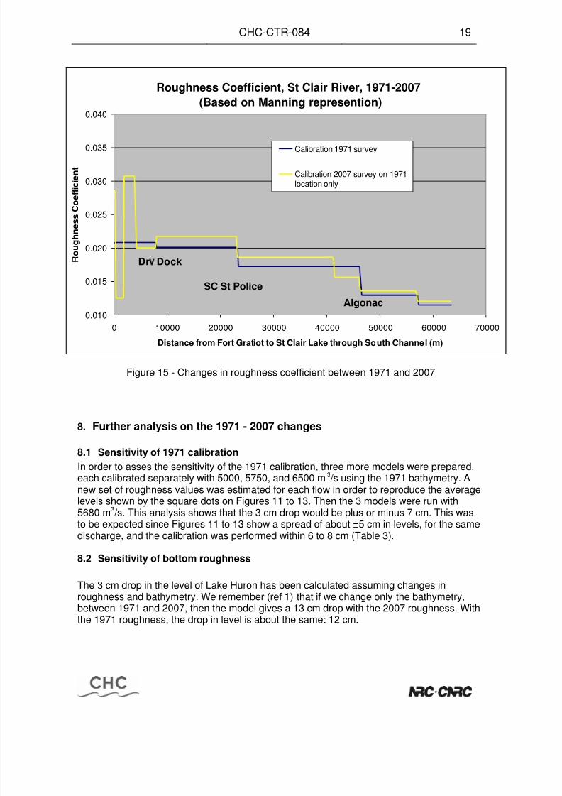
The coefficients representing the roughness of the river are shown in Figure 15. It showsthat in 2007 the roughness was slightly higher than in 1971. The average increase of theManning roughness coefficient over the whole length of the river is 5%. One explanation

could be that the increase would come from the removal of the finer material on the riverbed. Figure 15 also shows a regular decrease in roughness from upstream to downstream,coming probably from the fine material being transported and deposited where velocitiesslow down closer to the estuary.



CHC-CTR-084 19

Figure 15 - Changes in roughness coefficient between 1971 and 2007

8. Further analysis on the 1971 - 2007 changes

8.1 Sensitivity of 1971 calibration

In order to asses the sensitivity of the 1971 calibration, three more models were prepared,each calibrated separately with 5000, 5750, and 6500 m3/s using the 1971 bathymetry. Anew set of roughness values was estimated for each flow in order to reproduce the averagelevels shown by the square dots on Figures 11 to 13. Then the 3 models were run with5680 m3/s. This analysis shows that the 3 cm drop would be plus or minus 7 cm. This wasto be expected since Figures 11 to 13 show a spread of about ±5 cm in levels, for the samedischarge, and the calibration was performed within 6 to 8 cm (Table 3).

8.2 Sensitivity of bottom roughness

The 3 cm drop in the level of Lake Huron has been calculated assuming changes inroughness and bathymetry. We remember (ref 1) that if we change only the bathymetry,between 1971 and 2007, then the model gives a 13 cm drop with the 2007 roughness. Withthe 1971 roughness, the drop in level is about the same: 12 cm.

Roughness Coefficient, St Clair River, 1971-2007

(Based on Manning represention)

0.010

0.015

0.020

0.025

0.030

0.035

0.040

0 10000 20000 30000 40000 50000 60000 70000

Distance from Fort Gratiot to St Clair Lake through South Channel (m)

Roughness Coefficient

Calibration 1971 survey

Calibration 2007 survey on 1971location only

Algonac

SC St Police

Dr Dock



CHC-CTR-084 20

8.3 Sensitivity on 2007 discharges used in calibration

If we use a 2007 model calibrated with the existing EC relationship, without the additional

125 m3

/s, then we find that levels in Lake Huron would have risen by 3 cm since 1971instead of dropping by 3 cm. The net variation of 6 cm is close to what can be found onFigure 10, for 125 m3/s.

8.4 Sensitivity on 2007 bathymetry representation

As mentioned earlier, the density of the bathymetric data influences the numericalrepresentation of the bottom in the model.

A St. Clair river model was also prepared with the 2007 high density grid (6 and 10 m) —

instead of the 150 m spaced cross–sections — during calibration. With an upstream flow of5680 m3/s, this model also set the level of Lake Huron at 176.67 m, identical to the levelfound with the 2007 multi bean reduced to 1971 location (Table 6). This indicates that thehydrodynamics of the river remain the same if the model is properly calibrated with thesame set of bathymetric information.

But, it was found that the Manning friction coefficients for this 2007 model using highdensity bathymetric information were 12% higher than coefficients for the 2007 model usingthe low density 1971 locations.

8.5 Change in recirculation zone downstream of Blue Water Bridge

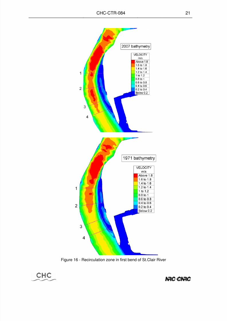
Since the bathymetry changed significantly between 1971 and 2007, a comparison wasperformed, with the Telemac models, of the velocity fields in the first bend downstream ofthe BlueWater Bridge, where a recirculation zone appears. In both cases the modeling wasdone with the Elder algorithm simulating the turbulence in the flow. Figure 16 shows that thelongitudinal location of the circulation has not changed since 1971 but it was about 40 mnarrower on its upper portion in 1971. This is confirmed by figure 17 and 18 which showcross sections of the water velocity profiles at four sections. (The sections are shown infigure 16).

These simulations were performed with the average conditions: 5680 m3/s flow from Lake

Huron with St.Clair Shores at 175.29 m



CHC-CTR-084 21

Figure 16 - Recirculation zone in first bend of St.Clair River



CHC-CTR-084 22

Figure 17 - Transverse section of water velocity profile (m/s), in sections 1 and 2



CHC-CTR-084 23

Figure 18 - Transverse section of water velocity profile (m/s), in sections 3 and 4



CHC-CTR-084 24

8.6 Comparison 1971 - 2007 volume of bottom sediments

Both 1971 and 2007 models were based on the same density of bathymetricinformation at the same locations along the river. It is therefore possible to compare

the change in volume of the two bathymetric surfaces as represented numerically inthe models (grid size of the order of 15 to 55 m).

Between 1971 and 2007 the following changes were measured:

• 29 cm average erosion in first section, 13 km down from Fort Gratiot

• 33 cm average erosion in middle section, next 16 km

• 20 cm average erosion in lower section, last 16 km to Algonac

Average erosion over the whole 45 km: 27 cm

These erosions were calculated as the volume change in the bottom over thesection, divided by the surface area of the section.

9. Effect of changing the location of a bathymetric survey

The 2007 multi-bean survey was applied only on the locations of the 1971 conventionalsurvey. What happen to the hydrodynamics of the River, if these locations are changedslightly, keeping the same density of survey points? To answer this question the followingprocedure was prepared:

• Reduce the 2007 multi-beam bathymetry to a regular grid (6 m upstream, 10 mdownstream of Black River as shown on fig. 9)

• Divide the SC River from Algonac to Fort Gratiot in 13 straight segments. Get thedirections of these segments

• Keep only the 1971 survey locations which fall within the 2007 Multi-beam survey

area (11366 points)• Within each segments, get the average 1971 cross section spacing

• Within each segment shift in the respective direction the X,Y coordinates of 1971survey location, by ½ the cross section spacing (see figures 19 to 22)

• On the new locations apply the 2007 multi-beam bathymetry. (weighted average of 4closest bathymetry points)

• Add the previously established 2007 bathymetry data for area close to shore lines,not covered by the 2007 Multi-beam survey (identical for all cases)

• Apply the bathymetry to Telemac grid

• Run Telemac model for 5680 m3/s upstream flow, and 175.29 m downstream level



CHC-CTR-084 25

• Repeat procedure for 3 cases:o No shifto Shifted in North directiono Shifted in South direction

Table 7 shows the hydrodynamic changes, while figures 19 to 22 show typical locations ofthe survey points. The last figure 23 shows a typical longitudinal cross sections (about 2.5km long) in all various cases, including the original section with the complete multi-beamsurvey.

No shift Shift NorthDifference

(m)Shift South

Difference(m)

Lakeport 176.804 176.817 0.013 176.805 0.001

Fort Gratiot 176.750 176.764 0.014 176.751 0.001

Algonac 175.479 175.477 -0.002 175.479 0.000

SC Shores 175.290 175.290 0.000 175.290 0.000

Table 7 - Changes due to shift in Bathymetric survey



CHC-CTR-084 26

Figure 19 - Stag Island shifted South

Black: location of original 1971 survey pointsColour: location shifted in South direction



CHC-CTR-084 27

Figure 20 - Stag Island shifted North

Black: location of original 1971 survey pointsColour: location shifted in North direction



CHC-CTR-084 28

Figure 21 - Bend upstream of Fawn Islands shifted South

Black: location of original 1971 survey pointsColour: location shifted in South direction



CHC-CTR-084 29

Figure 22 - Bend upstream of Fawn Islands shifted North

Black: location of original 1971 survey pointsColour: location shifted in North direction



CHC-CTR-084 30

Figure 23 - Resulting typical cross sections, after shift

Typical section: Difference in bottom representation in the numerical model.



CHC-CTR-084 31

10. Conclusion

The Elder algorithm simulating model turbulence gives a good representation of the large

recirculation downstream from Blue Water Bridge.

In order to assess the change in River hydrodynamics between 1971 and 2007, severalmodels were prepared. The accuracy of these models greatly depends on the quality of theinput data.

• The 1971 model was calibrated with errors in levels estimated at ± 7 cm

• The 2007 model was calibrated with errors in levels estimated at ± 1 cm

• Model calibration with steady state data provide better results than calibration withactual flow measurements (1 to 2 cm uncertainty instead of 5 to 13 cm)

• The uncertainty in flow measurements would provide level uncertainty of the order of± 6 cm

In these circumstances it was found that Lake Huron levels would drop by 3 cm between1971 and 2007 if the same constant inflow of 5680 m3/s was maintained and Lake St. Clairwas maintained at 175.29 m.

The major uncertainty is the flow estimates on which the Telemac models were calibrated.Recent ADCP surveys seem to indicate a discrepancy between flow measurements and theexisting stage-discharge relationships. We have assumed a 125 m3/s difference. If thedifference was 250 m3/s, then Lake Huron levels would have dropped about 9 cm.

11. References

1. Preparation of a hydrodynamic model of St. Clair River with Telemac-2D, to study

the Impacts of Potential Changes to the Waterway; Canadian Hydraulics Centre,

National Research Council, Ottawa, Ontario. March 2008, CHC-CTR-074

2. David Holtschlag, John Koschik, 2002. A Two Dimensional Hydrodynamic Model of

the St. Clair-Detroit River Waterway in the Great Lakes Basin, Detroit district, US

Army Corps of Engineers, report 01-4236

3. Jacob Bruxer, Aaron Thompson. St. Clair River Hydrodynamic Modeling, Using

RMA2, Phase 1 Report ; Prepared for the International Upper Great Lakes Study.

Environment Canada, March 2008.



CHC-CTR-084 32

4. David Holtschlag, John Koschik, 2005. Augmenting Two-Dimensional

Hydrodynamic Simulations with Measured Velocity Data to Identify Flow Paths as a

Function of Depth on Upper St. Clair River in the Great Lakes Basin;

U.S.Geological Survey, Scientific Investigations Report 2005-5081, 42 p

5. Personal communication with Aaron Thompson, Environment Canada, 8 January2008

canadian hydraulic centre

Documents