Can Regulators Allow Banks To Set Their Own Capital Ratios?

Lara Cathcarta, Lina El-Jahelb, Ravel Jabboura,∗

aImperial College London, South Kensington Campus, London SW7 2AZ, tel: +44 (0)20 7589 5111bThe Business School, University of Auckland, Private Bag 92019, Auckland 1142, New Zealand

Abstract

Basel regulators have received widespread criticism for failing to prevent two credit crises that hitthe U.S. over the last two decades. Nonetheless, banks were considerably overcapitalized prior tothe onset of the 2007-2009 subprime crisis compared to those which had undergone the 1990-1991recession. Therefore, if capital requirements were achieved prior to the subprime crisis, how couldthe Basel framework be blamed again for having accelerated if not caused another credit crunch?We find that the answer to this question lies in the relationship between the capital ratio and theleverage ratio which is governed by risk-weights categories determined by the Basel regulation. Weshow that changes to risk-weight categories which affect the correlation pattern between both ratiosare not reflected in the subprime crisis. This minimizes the implication of the Basel II regulationin the crunch that succeeded its announcement, in stark contrast to Basel I. We demonstrate thatthese dynamics are governed by a formula linking the two ratios together which derives from thesensitivity of the risk-based capital ratio to a change in its risk-weight(s). One implication of ourwork regarding the Basel III regulation consists in validating the newly established capital incre-ments in a mathematical rather than heuristical approach.

JEL classification: G21 G29

Keywords: Capital Ratio, Leverage, Basel

1. Introduction

The Basel Committee on Banking Supervision (BCBS) has been widely criticized for failing tomeet its bank safety objective after the U.S. witnessed two credit crunches in a span of less thantwenty years. Indeed, after the introduction of Basel I (BCBS (1988)), banks struggled to meetthe newly established risk-based capital requirements and hence shifted their portfolio compositiontowards safer assets to boost their capital ratios (CRs). This resulted in a lending contractionduring the 1990-1991 recession, hereafter referred to as the first crunch.

In contrast, since the Basel II framework was released (BCBS (2004) and BCBS (2006)), itseems that banks willingly increased their CRs beyond the target thresholds. According to Chamiand Cosimano (2010), in the early stages of the subprime crisis, the top 25 banks in the U.S.and Europe had a Tier 1 capital ratio of 8.3% and 8.1% while the Total capital ratio was 11.4%

∗Corresponding authorEmail addresses: l.cathcart@imperial.ac.uk (Lara Cathcart), l.eljahel@auckland.ac.nz (Lina El-Jahel),

r.jabbour10@imperial.ac.uk (Ravel Jabbour)

Preprint submitted to the Journal of Banking and Finance April 26, 2014

and 11.6%, respectively. Due to the distortionary incentives created by holding such high capitalbuffers (or moral hazard as indicated by Brinkmann and Horvitz (1995)), banks reached dangerousleverage ratios1 (LR) judging by the standards set by the main U.S. regulators (OCC, FDIC andFED) for well-capitalized institutions. Indeed, Gilbert (2006) states that up until mid-2005 onlythe two largest U.S. banks had a LR higher than 5%. Once defaults began their domino effectwhich triggered the second credit crunch in 2007-2009, the blame was directed at the regulatorsfor having incentivized banks to take on excessive risk prior to the crisis.

In sum, the effects of capital requirements have been investigated from two interconnectedperspectives. The first is related to the impact on lending growth (Bernanke and Lown (1991);Peek and Rosengren (1992, 1994, 1995a,b); Barajas et al. (2004); Cathcart et al. (2013b)) whereasthe second focuses on risk incentives (Koehn and Santomero (1980); Furlong and Keely (1987);Kim and Santomero (1988); Furlong and Keely (1989); Keely and Furlong (1990); Gennotte andPyle (1991); Shrieves and Dahl (1992); Calem and Rob (1999); Blum (1999); Montgomery (2005);Berger and Bouwman (2013)). Still, opinions remain mixed as to the effect capital can have ineach case, with different implications depending on the choice of variable used to measure capitaladequacy: Tier 1 VS Total (Demirguc-Kunt et al. (2010)).

Note that under each perspective, all but the last citations in our literature survey relate tothe first crunch. This underlines the greater attention attributed to the Basel regulation followingthis period. However, aside from minor changes to capital definitions, if the regulatory targetthresholds were maintained throughout the two decades at the pre-established 4% and 8% levelsfor Tier 1 and Total CR, any changes to CRs on the bank side would have been endogenous whilethe LR remained outside the scope of the Basel regulation. In principal, this would cancel out theregulatory effect on the second crunch.

Still, the latter effect could result from a more tacit change in the regulation, the introductionof new risk-weight categories. While the authors in our survey alternate between the use of the CRor LR when exploring the impact of capital, in this paper, we complement the existing literature byshowcasing that the two are not entirely independent. In fact, the two ratios are related throughchanges in the number of risk-weight categories which is exogenously determined by the regulators.This interaction between both ratios can lead to a new perspective on relating the abovementionedcrunches to the effects of capital requirements.

Our perspective relies on a four-step procedure. First, we motivate our discussion on the basisthat a shift in the banks’ binding constraint as witnessed between crises can be related to changesin risk-weights. In order to showcase the shifts in banks’ binding constraints between the twocrunches, we conduct a bank failure analysis in relation to the CR and LR requirements. Whileone might consider bank failure as being the adverse consequence of excessive risk-taking, not allfailures can be attributed to banks’ risky behavior with regard to capital adequacy2. Since theexisting literature investigated the causal linkages to the subprime crisis outside the realm of risk-based capital requirements (leverage, liquidity, securitization), our study re-emphasizes the effectsof these requirements on failures in an aim to fill the gap.

Second, we develop our theoretical framework which relies on a set of partial differential equa-

1Leverage is not to be confused with the traditional corporate finance definition as the ratio of debt to equity. Inthe regulatory context it is defined as the ratio of equity to assets (see section 2). In that sense, the higher the ratio,the safer the bank.

2Operational risk, for instance, has been at the helm of many investigations: fraud (Daiwa, Sumitomo), roguetrading (Barings Bank).

2

tions (PDE) related to the sensitivity of the CR which combines the two capital requirementstogether. The closed-form solution of this equation can assist policy-makers in setting adequaterather than heuristic targets for the CR and LR. This can also shed light on the controversyhighlighted by various authors (Hall (1993); Thakor (1996); Blum (2008); Buehler et al. (2010);Blundell-Wignall and Atkinson (2010); Kiema and Jokivuolle (2010)) regarding the effects of com-bining the two capital measures together under a single framework. In turn, this has implicationson the Basel III regulation which seeks to incorporate the LR as a “backstop” measure alongsidethe CR.

Third, we investigate the changes to the correlation patterns of LR and CR in order to givepreliminary evidence of the explanatory power of our framework. We show that these patterns arerelated to economic fundamentals such as lending and GDP which allows us to pinpoint the loancategory mostly correlated with the crunches.

Fourth, building on the previous step we provide empirical evidence of our model by analyzingits behavior over the two crunches. Our conclusions give support to the role of Basel I during thefirst crunch but discharges Basel II from any implication in regard to the second crunch.

Hence, in order to validate our four-step procedure we proceed as follows. In section 2, wedescribe our dataset. In section 3, we replicate the work conducted by Avery and Berger (1991)for the first crunch to illustrate the impact of CR and LR requirements on bank failures duringthe second crunch. In section 4, we develop our theoretical model linking the CR to the LR. Insection 5, we relate our theory to the correlation patterns which distinctively occurred during bothcrunches. In section 6, we validate our model from an empirical standpoint. We conclude with ourmain results and policy implications.

2. Data

Our dataset is based on FDIC Call Reports3 for the crunch periods 1990Q1-1991Q2 and 2007Q3-2009Q2. Ideally, in the case of exploring the regulatory impact following Basel I, we should havebegun in 1988; however, risk-weight data is only available as of 1990 which coincides with the startof the recession. Therefore in order to limit any bias between the periods and for comparativepurposes, we restrict the second period also to the subprime crunch period4.

Both CR and LR are proportional to Tier 1 capital by definition5. After discarding all negativeCR6 values, we construct various sub-samples of the dataset based on the distribution of the CR.The latter range from the 90th to the 50th percentiles. Our choice of 90% cutoff value relates toremoving the effect of outliers mostly located in the upper percentiles of the data, while the limit of50% is used to maintain a reasonable amount of observations. Descriptive statistics for the upperand lower bounds of the sub-samples are shown in Table I.

The survivorship bias is apparent in our study as can be seen from the reduction in the numberof banks between both periods. However, as the higher moments of the data are fairly similar

3Also known as Reports of Condition and Income taken from the Federal Financial Institutions ExaminationCouncil (FFIEC).

4We will show in section 6.2 that this restriction does not impact our result in relation to the actual implementationdates for the respective Basel regulations.

5With reasonable approximation based on the risk-based capital definitions for Prompt Corrective Action (PCA)as posted by the FDIC, CR = K/RWA; LR = K/A where K is Tier 1 Capital. See Theory section for more details.

6The formulae in this study imply that the CR and LR should be positive.

3

between the two periods, our sample is not affected by the bias. Furthermore, we witness anorder of magnitude increase in the value of (risk-weighted) assets due to balance-sheet expansions,mergers and acquisitions. In particular, mortgage lending, which played a key role in both crises,witnessed an important increase.

Table I:Summary Statistics

The data in this table relates to the beginning of each designated crunch period, 1990Q1 and2007Q3. Values are shown after winsorizing the data with respect to the CR at the 90th and 50thpercentiles. Risk-weighted assets (RWA), Total Assets (TA) and Mortgage Assets (A) are in USD.

Panel A: 1990Q1

Pct 90% 50%

Var Obs Mean Std Dev Skew Kurt Obs Mean Std Dev Skew Kurt

CR 12069 12.5 4.3 0.5 3.0 6714 9.5 2.1 -1.2 4.7LR 12069 8.0 2.5 1.8 33.1 6714 6.7 2.0 5.2 155.2

RWA 12069 2.58 2.69 45.8 2903.8 6714 3.98 3.49 34.5 1636.1TA 12069 3.18 2.59 34.9 1731.8 6714 4.88 3.39 26.6 997.0A 12069 1.08 7.78 30.3 1198.2 6714 1.68 1.09 23.3 697.5

Panel B: 2007Q3

Pct 90% 50%

Var Obs Mean Std Dev Skew Kurt Obs Mean Std Dev Skew Kurt

CR 7729 14.4 4.9 1.1 3.6 3838 10.7 1.3 -0.4 4.0LR 7729 10.3 3.1 2.0 9.6 3838 8.6 1.3 0.6 8.3

RWA 7729 12.38 20.49 38.2 1630.3 3838 22.48 28.89 27.2 823.9TA 7729 15.48 26.09 40.4 1804.4 3838 27.38 36.89 28.8 910.8A 7729 6.08 76.48 33.2 1331.2 3838 10.38 10.69 24.4 709.9

Moreover, the CR and LR statistics which increased by around two percentage points allow us tore-assert the finding in Chami and Cosimano (2010) that banks were indeed better capitalized beforethe second crunch compared to the first. This could have happened either through a voluntaryincrease in capital by banks, or involuntarily through changes to risk-weights.

One conclusion that can be made from our data inspection is that had the regulators linkedthe CR and LR together by any linear association (for instance, CR - LR > Constant), we wouldexpect similar distributions for each ratio. However, this is not the case as can be seen at the90th percentile7 with the quasi-normal distribution of the CR (Skewness ≈ 0, Kurtosis ≈ 33)versus a positively skewed and leptokurtotic distribution for the LR (Skewness ≈ 2, Kurtosis variesaccording to the period) during the first crunch. This indicates the presence of a non-linear, if any,linkage between the two ratios.

3. Motivation

The CR and LR are the most popular measures of capital adequacy. In view of the commoncapital feature embedded in both ratios, any changes between the CR and LR can be attributedto changes in their denominators, risk-weighted versus unweighted assets. However, each of thetwo ratios can have very different effects on a bank’s behavior depending on which of the two is

7The sample distribution is no longer normal at the 50th percentile.

4

the binding constraint (Berger and Udell (1994), Hancock and Wilcox (1994), Peek and Rosengren(1994), Chiuri et al. (2002), Barajas et al. (2004), Blundell-Wignall and Atkinson (2010)).

Two studies which investigated the impact of the CR and LR on bank failures during the firstcrunch are Avery and Berger (1991) and Estrella et al. (2000). Although the latter study cameat a much later time than the former, it only pointed out the critical regions at which banks wereaffected by one ratio or the other. Hence, no consideration was given to the combined effect ofthe two ratios. However, one important observation we make from the authors’ results is that atleast one year prior to its failure, a bank can have the same LR in the critical region as one whicheventually survived. This supports the fact that the LR has no predictive power regarding bankfailures in contrast to the CR, in line with the authors’ conclusion. However, it is important tomake sure this statement remains valid during the second crunch.

Avery and Berger (1991) make a similar assessment by which they calculate the number ofbanks that went bankrupt just before the start of the first crunch given that these banks hadearlier failed to meet one or more of the CR and/or LR regulations. For example, almost a third ofthe 6% of banks which could not meet the targets for Tier 1 capital, Total capital or leverage failedover the next 2 years8. More importantly, 50% of all banks failing the Tier 1 target eventuallywent bankrupt, putting this requirement at pole position in terms of forecasting power.

Following the same line of thought as the previous authors we analyze the relationship betweenthese capital standards and bank failures for the second crunch. This complements findings suchas those of Berger and Bouwman (2013) who observed that a one standard deviation decrease incapital more than doubles the probability of bankruptcy. However, their result shows this relationas being linear even though authors which differed on their assessment of risk and capital (Koehnand Santomero (1980); Furlong and Keely (1987); Kim and Santomero (1988); Furlong and Keely(1989); Keely and Furlong (1990)) still agreed that capital shortfalls weigh more on a bank’s survivalrate than surpluses.

Notwithstanding some components might have changed, the CR targets were not altered be-tween the two Basel frameworks. This allows for a direct comparison with Avery and Berger(1991). Nonetheless, instead of exploring changes before and after the Basel II capital standardswere brought in, our study uses three intervals (pre, mid and end of the crisis), in order to gaugethe evolution in meeting these standards along with the leverage requirement as the crisis unfolded.

Unlike the fixed CR targets, the choice of which LR is chosen to compare between banks is ateach author’s discretion. This is because CAMEL ratings, which guide national regulators in theirdiscretionary LR requirement for each bank, are not disclosed9. Both Avery and Berger (1991) andHall (1993) chose the minimum leverage target of 3% for their analysis which could be the reasonthey amount to similar conclusions on the binding effect of capital rather than leverage ratios. Inthe latter author’s own words, if the average LR were assumed at 3%, the CR becomes the morelikely first crunch culprit since most banks are able to fulfill the LR requirement. However, if theLR were established at a level of 5% then at least 18% of these would fail the leverage target.In order to circumvent these issues, we look at a range of leverage targets 3%, 4% and 5% andmaintain that our results are valid at each level. Finally, we look at how combinations of both

8Note that in the Basel framework, if a bank fails Tier 1 it automatically fails the Total requirement as theregulators impose that Tier 2 cannot exceed 50% of Tier 1.

9Under this rating scheme, the safest banks, attributed the best rating of 1, are given a leverage target of 3%.Depending on their condition, all other banks are set a target of either 1 to 2 percentage points higher. Even if itwere known, the function underlying the “CAMEL-to-Leverage” specification is arguably not bijective.

5

standards impact on bankruptcies.Table II shows a number of compelling findings. Bearing in mind that banks were transiting

from the 1980’s flat rate system to Basel I requirements, we recall that Avery and Berger (1991) hadobtained a 94% estimate of the proportion of banks that passed all three requirements prior to thefirst crunch. In contrast, banks did not have to modify their capital thresholds after Basel II, whichexplains the higher proportion of compliant banks (99%) at the onset of the second crunch. Thisvalidates the similar estimates obtained by Greenspan et al. (2010). Another difference betweenthese periods is that the non-compliant banks accounted for a quarter of total assets according toAvery and Berger (1991). Based on Berger and Udell (1994), this amounted to a 20% increase inbanks not abiding by the regulation. In contrast, non-compliant banks were less than 1% in termsof total assets during the post-Basel II period which reinforces the idea that very few had actuallyfailed the standards.

Nevertheless, failing any of the standards in the latter period had more serious repercussionssince a much greater proportion of the pre-crunch bank pool ended up bankrupt. Ultimately, allbanks failing either the Tier 1 CR or a 3% LR in the pre-crisis period went bankrupt. Moreover,we point out the increase in the failure to meet any of the requirements over time. This contrastswith a simultaneous decrease in bankruptcy rate, specifically between the start and end of theobservation period. The first finding stresses the weakened capital position of banks eroded bylosses throughout the crunch period. The second finding relates to corporate finance theory inthat survival rates increase for banks which can endure more phases of a crunch (Klapper andRichmond (2011)).

A striking feature is that during all three phases of the crunch, all banks that failed Tier 1,and obviously Total, capital ratios also failed the LR requirement of 4%. As a matter of fact, fromthe same proportion of banks which ended up bankrupt prior to the crunch, more banks had failedbecause of the minimum 3% LR rather than the CR requirement. This has crucial implications onBasel III as it brings back into question the purpose of imposing dual requirements, suggesting thatthe BCBS’ decision of imposing a backstop 3% requirement could be overly conservative. Whilethe implications from failing the CR in terms of bankruptcy were higher for the CR compared tothe LR requirement at the peak of the crisis (2008Q2), this is not sufficient to rule out leverageas the binding constraint on banks as increasing the target by 1% always resulted in an averagedoubling of the failure rate to meet the requirement across all periods (above 1% failure rate forthe 5% target).

Moreover, when quantifying the magnitude of failing a specific standard one must relate itto surpluses, or alternatively shortfalls10. As a matter of fact, Brinkmann and Horvitz (1995)emphasize that regulators should not only look at how many banks are likely to fail a newlyintroduced standard but also by how much their (excess) capital cushion would vary11. Hence,one motivation for performing the following study is to assess the adequacy of the new Basel IIIstandards.

10Focusing on shortfall is arguably a better choice then surplus. Firstly because, the fact that banks were overlycapitalized prior to the crunch did not fare well for some of them during the crunch. In other words, while thecapital buffer size does matter for the regulators, it does not reflect quality of capital. This means that surplus couldbe a biased signal for the health of the banking sector. Secondly, shortfall is more amenable to the idea of settingminimum capital requirements.

11Regulators classify institutions into four main capital surplus/shortfall categories: Adequately/Under capitalizedand Significantly/Critically undercapitalized.

6

Hence, in the same spirit as Hancock and Wilcox (1994), we calculate the average shortfall asthe sum of differences between the target ratio and the actual ratio divided by the number of non-compliant banks. Shortfall turned out to be equal to 1.5% for Tier 1 capital which is actually inline with the current steps taken by the BCBS to increase the Tier 1 requirement by 2%. However,the BCBS decision to abide by the 3% leverage requirement could end up short of expectations asour analysis reveals that the shortfall of 0.5% could double if the target was increased to 4%. Thissuggest a review of the CAMEL ratings system to reflect the median bank’s behavior during crisesperiods.

While it is difficult to ascertain which of the two ratios was the binding constraint on bankspurely on the basis of failure and shortfall analysis, one definite conclusion is that compared to thestatistics in Avery and Berger (1991), the LR played a much more important role for this crunch.This is in contrast with the first crunch where banks were mostly struggling to meet their CRrequirements. Hence, our conclusion statistically corroborates the statements in Gilbert (2006)12

and Blundell-Wignall and Atkinson (2010).On reflexion, Furfine (2000) claims that the same magnitude change in either ratios can lead to

drastically opposite effects in terms of portfolio risk. In fact, Gilbert (2006) suggests that changingthe risk-weights in the CR would impact the number of banks bound by the LR despite the fact thatthe latter is insensitive to risk-weights by definition. More specifically, using the exact scenario thatoccurred prior to the subprime crunch, in other words a reduction in the risk-weight attributed tofirst-lien residential mortgages13, the author shows that a risk-weight lowering lead to an increasein the number of banks bound by the LR. The latter is achieved by moving banks further from theCR constraint without changing the distance to the LR constraint. As a result, when capital isreduced due to loan losses, the first constraint that banks would hit is the LR requirement. Thishypothesis has fueled our incentive to explore the interaction between the CR and LR from theperspective of risk-weight changes.

Table II:Bankruptcy Predictions from Banks Failing to Meet Various Capital Standards

Our results for the period 2004Q3-2009Q2 are broken down into three consecutive dates (pre,mid, end of crisis). With regard to the overall sample, we account for the bank percentagein terms of number (%B) and assets (%A). Each row consists of a different regulatory target.Numbers in brackets are for use in the last rows as combinations of the previous singlestandards where ‖ denotes the logical OR and & is the logical AND. The last row is for bankswhich passed all standards (with a 3% LR). In that case, the following identity can be applied:Prob[Pass] = 1 - Prob[(1)‖(2)‖(3)].

Pre-crisis (2007Q2) Mid-crisis (2008Q2) End-crisis (2009Q2)

Standard %B %A %Bkrpt %B %A %Bkrpt %B %A %Bkrpt

Tier1-CR(1) 0.02 0.00 100.00 0.10 0.25 88.89 0.49 0.37 30.23Total-CR(2) 0.10 0.12 55.56 0.25 0.11 63.64 0.94 0.37 12.203%-LR(3) 0.03 0.02 100.00 0.09 0.01 62.50 0.47 0.31 31.714%-LR(4) 0.07 0.05 66.67 0.15 0.25 46.92 0.89 0.45 27.275%-LR(5) 0.14 0.15 69.23 0.39 0.34 42.86 1.42 0.85 17.89(1)‖(2)‖(3) 0.12 0.12 63.64 0.37 0.35 66.67 1.44 0.74 18.40(1)&(2)&(3) 0.02 0.00 100.00 0.07 0.00 83.33 0.43 0.30 32.43

Pass 99.86 99.85 7.02 99.63 99.65 3.38 98.55 99.26 0.49

12Though the author uses a different definition for the binding capital requirement based on surpluses rather thanthe actual number of banks that achieved the given target.

13Although the author’s specification changes the original value of 50% to half its value, rather than the one chosenby Basel of 35%.

7

4. Theory

In this section, we undertake a mathematical approach in order to assess whether the two ratios,LR and CR, are inter-related. The equations presented here will be important for the derivationswe conduct at a later stage.

According to the Basel framework, risk-weighted assets are defined as the weighted sum ofassets on a bank’s balance sheet, where the weights are attributed according to the asset’s creditrisk. Hence, denoting K as Tier 1 capital, the ratio of Risk-Weighted Assets (RWA) to TotalUnweighted Assets (TA) in equation (1) is commonly used as a measure of risk as it is boundbetween 0 and 1 in increasing order of credit risk. This is because RWA tends towards TA as theproportion of risky assets (high risk-weight) increases. Therefore, what is not noted in most of therecent literature which uses this credit risk proxy (Van-Roy (2005), Hassan and Hussain (2006),Berger and Bouwman (2013)) is that it is equivalent to an interaction between the CR and LR,irrespective of capital K14.

RWA

TA=

KCRKLR

=LR

CR(1)

Moreover, it is apparent from equations (2) and (3), that the more a bank invests in the assets(Ai), in the limit where all assets belong to the lowest risk-weight category (wi = 0) the CRconverges to infinity. In other words, the CR is not affected by changes to assets unlike the LRwhich always moves with the level of assets. The two ratios are expected not to be correlated inthis case. In contrast, in the limit where all assets belong to high risk-weight categories (wi = 1),the CR will decrease until it coincides with the LR. In sum, the two ratios are correlated dependingon the overall level of risk-weights.

limwi→0

CR = limwi→0

K∑Ni=1wiAi

=∞ = Cte (2)

limwi→1

CR = limwi→1

K∑Ni=1wiAi

=K∑Ni=1Ai

= LR (3)

4.1. Deriving the relationship between CR and LR

In similar spirit to Van-Roy (2005) and Hassan and Hussain (2006)15, the change in CR isderived with respect to a change in risk-weight, wi, affecting a certain asset category i out of a poolof N categories16.

First, as can be seen from Equation (5), this change is negatively related to the product ofthe CR and a second term which is dubbed “asset proportion” (APi). This term refers to the“proportion” of asset whose risk-weight is being changed towards the total amount of risk-weightedassets.

14Kamada and Nasu (2000) are the closest to reach this result as they use Total capital in the definition of the CRversus Tier 1 capital for the LR. This leads to a different but related concept: the asset quality index.

15These authors derive changes with respect to CR itself, i.e. CR growth rather than with respect to a change inrisk-weight.

16Prior to Basel II, N=4 for i∈[0, 20, 50, 100].

8

δCR

δwi=

δ

δwi

(K∑N

j=1wjAj

)= K × δ

δwi

(1∑N

j=1wjAj

)

= −K ×

(Ai

(∑N

j=1wjAj)2

)= − K∑N

j=1Aj

×∑N

j=1Aj∑Nj=1wjAj

× Ai∑Nj=1wjAj

= −LR× 1RWATA

× Ai

RWA(4)

= −LR× 1LRCR

×APi = −CR×APi (5)

Since the product of terms is always positive, the change in CR resulting from a positive changein wi is always negative. The intuition lies in the fact that an increase in risk-weight means morerisky assets which implies a negative (positive) shock to the CR numerator (denominator) result-ing in an overall decrease. This statement has policy implications with regard to one prominentexample which occurred during the transition from Basel I to Basel II as the risk-weight on res-idential mortgages fell from 50% to 35%, respectively (Blasko and Sinkey (2006) and Cathcartet al. (2013b)). Seemingly without anticipating the artificial increase this change would have onCRs, regulators maintained the same CR targets despite lowering the risk-weight17. In fact, theyshould have increased the CR targets even further to maintain adequate capital buffers. Whilesome might argue that this strategy could have exacerbated the crunch by increasing the contrac-tion in lending, it might have proven worthwhile in weathering it by having forced banks to holdhigher loss-absorption layers. Arguably, this has been taken into consideration under Basel III inthe setting of the new CRs.

Second, another interesting feature which is apparent from equation (4) is that the sensitivityof the CR to a change in risk-weight is higher in absolute terms the higher the LR, the safer thebank in terms of credit risk (low RWA/TA), and the larger the affected asset proportion (APi).Hence, equation (4) provides the mathematical framework to highlight the importance of the creditrisk ratio and asset proportion in dampening or intensifying the sensitivity of the CR. Note thatthe reason why the safest banks are the most sensitive to changes in CR can be understood in thecontext of an extreme scenario where the risk-weights are at zero. In that case, the CR is immuneto changes in any amount of assets. However, any deviation in risk-weight away from zero is likelyto perturb it significantly.

So far, our derivations have highlighted the dependence of the CR on the LR, affected by anegative sign for the case of a change with respect to a single risk-weight category, wi. It is easy toshow that the relationship between the CR and LR can be extended to all N categories which yieldsthe following formulae in equations (6) and (7). We notice that most terms were adapted fromthe previous single risk-weight case, with the last factor being the product of asset proportions.Our focus, however, is on the preceding negative sign, which now changes to a sinusoidal patternof positive/negative signs depending on the number of risk-weight categories. This captures, along

17Unless other risk-weight changes had, in their view offsetting effects.

9

with the factorial term18, the interactions between different changes in risk-weights.

δCR

δw1...δwN= (−1)N ×N !× LR× 1

RWATA

×N∏i=1

APi (6)

= (−1)N ×N !× CR×N∏i=1

APi (7)

Note that the behavior of the function in the CR sensitivity equations is undetermined as Ntends to infinity. However, this is not an issue for a few number of risk-weight categories as isnormally the case. Moreover, while the correlation between LR and CR is always positive, thesensitivity of the CR, as captured by its derivative(s) could vary depending on the total numberand sign (positive/negative) of all possible changes affecting the risk-weight categories. This shouldalways be taken into account by regulators when changing any of the constituents of the CRsensitivity. More importantly, for given change(s) in risk-weight(s), these formulae allow us toinfer the necessary change in CR holding constant the changes in these constituents.

Finally, based on these formulae, we conjecture that the introduction of the risk-weight schemeunder Basel I took N from one to four, triggering a change in the sign of the sensitivity of theCR. As such, the average risk-weight would have fallen from 1 to an arbitrary W̄ . This makesthe change in wi negative, resulting in a fall in CR for a positive change in LR. Thus the tworatios would vary in opposite ways, bringing down the correlation between them. In contrast, thefour new risk-weights introduced under Basel II19 which would have taken N to eight would nothave altered the sign on the sensitivity of the CR even if they had been fully implemented. Animplication of this would be to minimize the role of the Basel regulation in relation to the crisis.

5. The Change in CR and LR Correlation Patterns

Before moving to the empirical validation of our theoretical findings, we elaborate further onthe correlation patterns for the CR and LR during the distinctive periods of post-Basel regulations.

5.1. Pattern Reversals and Economic Fundamentals

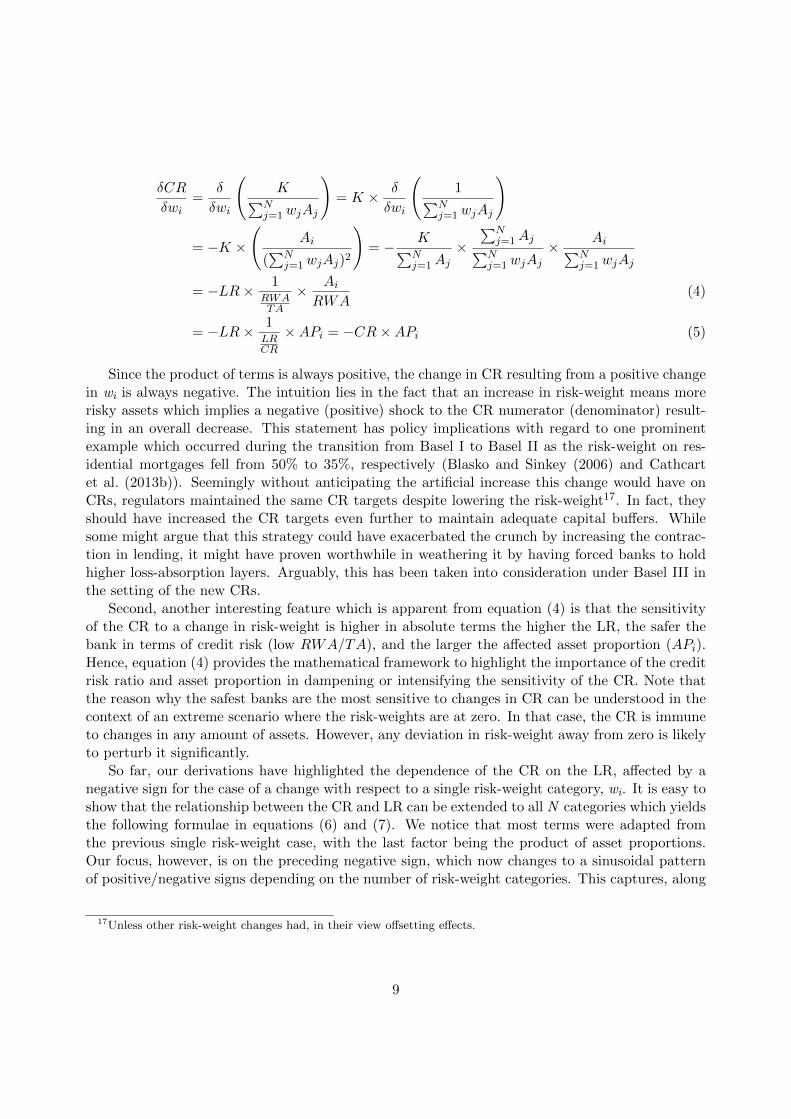
In this section, we illustrate the changes in LR and CR co-movement patterns in each crunchperiod. Our correlation estimates are calculated on the basis of the 90th percentile sample in TableI and plotted in Figures 1 and 2 for each period, respectively.

Note that various authors have measured this correlation over a single period without mention-ing if the resulting pattern is likely to be persistent over time. For instance, Estrella et al. (2000)perform their calculations for the first crunch only. Their yearly values coincide to a large extentwith the ones we obtain for the first quarter of each year in Figure 1. To our knowledge, they werethe first to have observed an imperfect time-varying correlation pattern between the two capitalmeasures which hints to the fact that each ratio can provide independent information on capitaladequacy for a given bank.

As such, the key point of our analysis is with regard to changes in the correlation patternsfor each of the crises. During the first crunch (Figure 1), it would seem as though the correlation

18This term arises from the successive derivations with respect to the risk-weights.19Those were 35%, 75%, 150% and 300%.

10

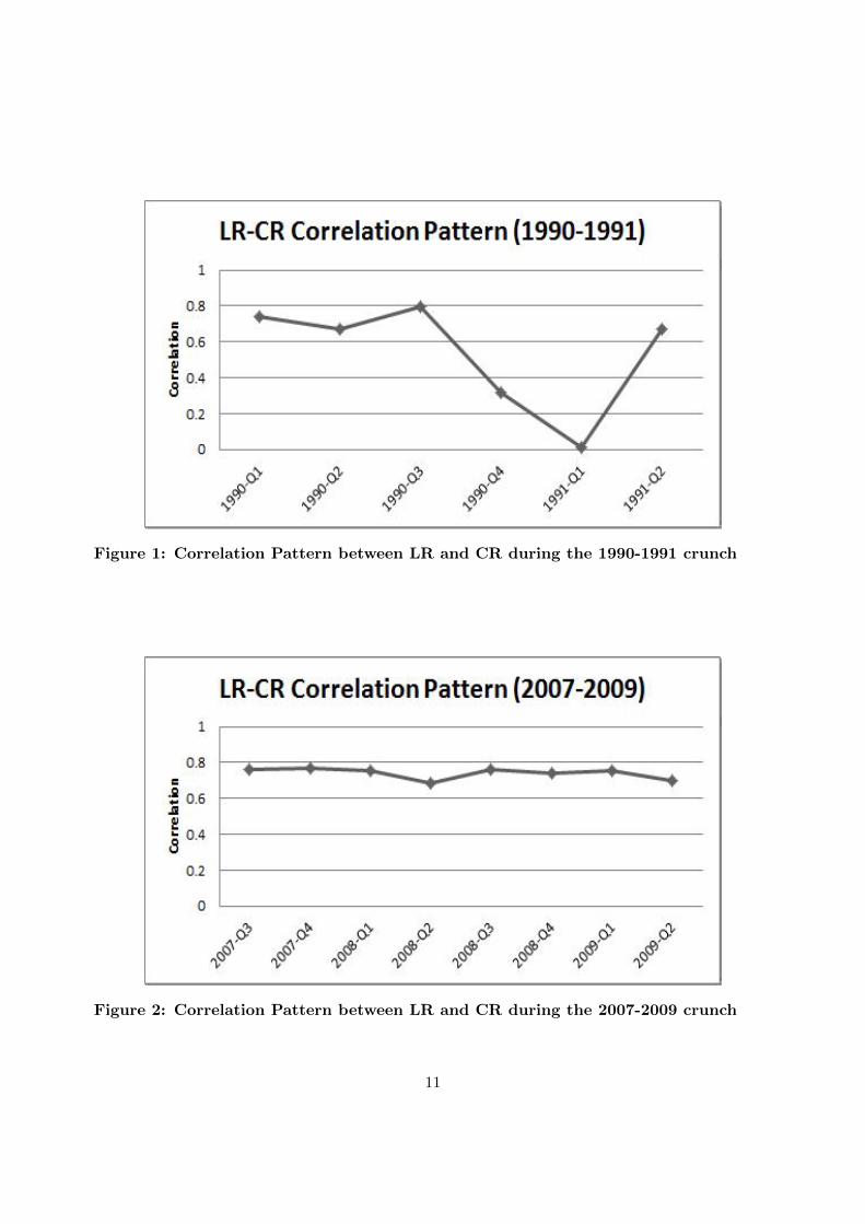
Figure 1: Correlation Pattern between LR and CR during the 1990-1991 crunch

Figure 2: Correlation Pattern between LR and CR during the 2007-2009 crunch

11

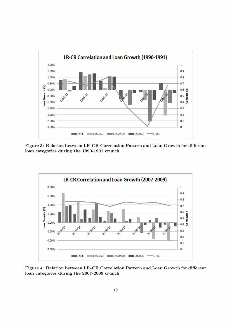
Figure 3: Relation between LR-CR Correlation Pattern and Loan Growth for differentloan categories during the 1990-1991 crunch

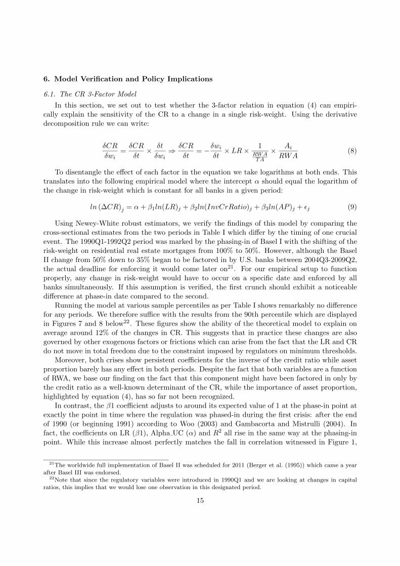
Figure 4: Relation between LR-CR Correlation Pattern and Loan Growth for differentloan categories during the 2007-2009 crunch

12

Figure 5: Relation between LR-CR Correlation Pattern and GDP during the 1990-1991 crunch

Figure 6: Relation between LR-CR Correlation Pattern and GDP during the 2007-2009 crunch

13

fluctuates around 0.75 in the first few quarters of the crunch. It then falls sharply between 1990Q4-1991-Q1 before reverting to its previous level. In contrast, during the second crunch, the patternremains at 0.75 with no noticeable changes (Figure 2). Note that the presence of a fall during thefirst (and shorter) crunch is hinted to by the fact that the change in correlation between peak andtrough is around ten times that in the second crunch.

In addition, it seems as though the LR-CR correlation pattern during the first crunch is morecorrelated with microeconomic and macroeconomic fundamentals, such as loan growth (0.75 versus0.43) and GDP (0.66 versus 0.37), than during the second crunch. As in Berger and Udell (1994)and Shrieves and Dahl (1995), we categorize lending growth into three major groups belong-ing to high-weighted risk categories (50%-100%): real estate (LNRE), commercial and industrial(LNCIUSD) and consumer (LNCONOTH) loans. We also include the aggregate (LNSGR). As isapparent during the first crunch, the correlation pattern is strongly associated with the overall20

lending pattern (Figure 3). That is not the case during the second crunch (Figure 4). Hence, thisfavors a change in the dynamics between the two ratios and lending only during the first crunch.Such a change could be a result of changes in the high-risk weight categories which affect thecorrelation between the LR and CR as seen in equation (3).

Similarly, with regard to GDP, in line with the positive relationship between lending and GDPas established in Gambacorta and Mistrulli (2004), one could argue that in a financial crisis, macroeffects take longer to appear in the economy than at the micro-banking level. For this reason, weuse a one-quarter lagged LR-CR pattern instead of the concurrent one and plot it alongside GDPin Figures 5 and 6. The results are similar in comparison to loan growth. In sum, this highlights anew finding that the correlation between CR and LR can be considered as an economic signal asit reflects the lending and economic cycles.

Finally, we capture the loan category mostly linked to each of the crises by computing thecorrelation of each category with the LR-CR correlation pattern. The results for each categoryare shown in Table III. The correlation of the LR-CR pattern with real estate lending is perfectlyin line with the overall loan portfolio (LNSGR) during the first crisis when this category receiveda lower risk-weight than the rest (50%). During the second crunch, it even surpasses the rest ofthe three categories at a time when it received a second round lowering to 35%. This illustratesthe differential role this asset class played during each crunch. We refer to this in our empiricalsection.

Table III:Correlation between ρ and Loan Asset Growth

The results in this table refer to the correlation betweenvarious loan asset classes and the observed LR/CR patternfor each designated crunch period.

Loan Asset Crunch 1 Crunch 2Class (1990Q1-1991Q2) (2007Q3-2009Q2)

LNRE 0.75 0.59LNCIUSD 0.30 0.41

LNCONOTH 0.84 0.14LNSGR 0.75 0.43

20Although one cannot infer from observing these figures which of the loan growth categories is mostly correlatedwith the LR-CR pattern, the lending contraction is obvious in both figures. We look at the individual categoriesnext.

14

6. Model Verification and Policy Implications

6.1. The CR 3-Factor Model

In this section, we set out to test whether the 3-factor relation in equation (4) can empiri-cally explain the sensitivity of the CR to a change in a single risk-weight. Using the derivativedecomposition rule we can write:

δCR

δwi=δCR

δt× δt

δwi⇒ δCR

δt= −δwi

δt× LR× 1

RWATA

× Ai

RWA(8)

To disentangle the effect of each factor in the equation we take logarithms at both ends. Thistranslates into the following empirical model where the intercept α should equal the logarithm ofthe change in risk-weight which is constant for all banks in a given period:

ln (∆CR)j = α+ β1ln(LR)j + β2ln(InvCrRatio)j + β3ln(AP )j + εj (9)

Using Newey-White robust estimators, we verify the findings of this model by comparing thecross-sectional estimates from the two periods in Table I which differ by the timing of one crucialevent. The 1990Q1-1992Q2 period was marked by the phasing-in of Basel I with the shifting of therisk-weight on residential real estate mortgages from 100% to 50%. However, although the BaselII change from 50% down to 35% began to be factored in by U.S. banks between 2004Q3-2009Q2,the actual deadline for enforcing it would come later on21. For our empirical setup to functionproperly, any change in risk-weight would have to occur on a specific date and enforced by allbanks simultaneously. If this assumption is verified, the first crunch should exhibit a noticeabledifference at phase-in date compared to the second.

Running the model at various sample percentiles as per Table I shows remarkably no differencefor any periods. We therefore suffice with the results from the 90th percentile which are displayedin Figures 7 and 8 below22. These figures show the ability of the theoretical model to explain onaverage around 12% of the changes in CR. This suggests that in practice these changes are alsogoverned by other exogenous factors or frictions which can arise from the fact that the LR and CRdo not move in total freedom due to the constraint imposed by regulators on minimum thresholds.

Moreover, both crises show persistent coefficients for the inverse of the credit ratio while assetproportion barely has any effect in both periods. Despite the fact that both variables are a functionof RWA, we base our finding on the fact that this component might have been factored in only bythe credit ratio as a well-known determinant of the CR, while the importance of asset proportion,highlighted by equation (4), has so far not been recognized.

In contrast, the β1 coefficient adjusts to around its expected value of 1 at the phase-in point atexactly the point in time where the regulation was phased-in during the first crisis: after the endof 1990 (or beginning 1991) according to Woo (2003) and Gambacorta and Mistrulli (2004). Infact, the coefficients on LR (β1), Alpha UC (α) and R2 all rise in the same way at the phasing-inpoint. While this increase almost perfectly matches the fall in correlation witnessed in Figure 1,

21The worldwide full implementation of Basel II was scheduled for 2011 (Berger et al. (1995)) which came a yearafter Basel III was endorsed.

22Note that since the regulatory variables were introduced in 1990Q1 and we are looking at changes in capitalratios, this implies that we would lose one observation in this designated period.

15

Figure 7: Three Factor Model for the CR sensitivity to a change in Risk-Weightduring 1990Q2-1992Q2

Figure 8: Three Factor Model for the CR sensitivity to a change in Risk-Weightduring 2004Q3-2009Q2

16

there is no such perceivable change for the second crunch as seen from Figure 2. This almostcertainly suggests that the Basel regulation was implicated in the first crunch but not the secondthrough the changes in risk-weights which accompanied the new CR. In other words, the trough inFigure 1 which is almost 0, refers to the lowest possible correlation between LR and CR. Accordingto equation (2), this relates to a period in which banks accumulated safe assets, in the form ofTreasury Bills ((wi = 0), and as a result cut-down on lending which lead to the crunch.

In addition, we observe a significant value of 4.3 at 1% for the unconstrained α (Alpha UC) in1991Q1 which is almost twice as high as the ones obtained throughout the corresponding period.However, despite also being significant, our value of 4.6 changes relatively little during the secondperiod and does not exhibit the same noticeable change as in the first period. Assuming the onlyrisk-weight change that took place in both periods was related to residential mortgage assets, themodel derivation in equation (9) implies that we should detect an α of 3.9 (2.7) for the first (second)period23. Clearly, the expected value corresponding to the first crunch is much closer to the model-implied value which re-asserts the changes in risk-weights which happened at that time. In anycase, the exact values could not have prevail owing to the fact that our formula is not enforcedby the banking industry. Nonetheless, the comparison between both periods confirms that banksratios still account for instantaneous changes in risk-weight which our model is sensitive to.

Note that our empirical findings are only valid for changes in a single risk-weight which couldnot always be the case. Our results could have therefore been affected by disturbances fromunaccounted changes. Hence, we force the theoretical constraint that all coefficients be equal to1 in equation (9). On one hand, the constrained α (Alpha C) in the first period still undergoesa perceivable change in 1991Q1. This indicates that our constrained model remains sensitiveto changes that occurred during this period. On the other hand, while the constrained α in thesecond period is almost the same as its expected value at around 2.4, the fact that it remains almostconstant over time suggests again that banks did not undertake a specified change in risk-weightduring the second crunch.

6.2. Linking the CR to the LR: Policy Implications

In this section, we derive a framework for explicitly setting the CR with respect to the LR. Ourstarting point is equation (7) which is a simple homogeneous partial differential equation (PDE)that can be solved in closed form. The derivations are stated in the Appendix. In the case of asingle risk-weight change, the relationship becomes:

CR = LR× e∑N

i [APi(1−wi)] (10)

As the exponential power term is always positive, the CR should always be greater than theLR. Indeed, the formula implies that banks should at least meet a lower threshold of CR equal toLR; afterwards, they should increment their respective risk-based capital positions by a weightedaverage of their asset proportions as captured by the exponential term in equation (10). Forexample, with a 3% LR, the old Tier 1 CR of 4% is reasonable but for the less conservative LR of5% it is not. Indeed, such distortions to the above identity could induce wrongful behavior on thepart of banks as was reported in Gilbert (2006). Hence, as the CR is set to increase to 6% underBasel III, this is in line with both LR targets between 3-5%.

23These values are equivalent to ln(-(50-100)/1) and ln(-(35 - 50)/1).

17

In the following, we test to what extent equation (10) holds empirically using the followingpanel regression. Our results are shown in Table IV.

ln

(CR

LR

)jt

= α+ βN∑i

[APi(1− wi)]jt + εjt (11)

We report that across the two sample periods all estimates are significant at the 1% level. Ascan be seen from panels A and B, at the 90th (95th) percentile, the R2 increases to 93% (77%) forthe first (second) crunch. The relationship then weakens the smaller our sample becomes as thismakes it more specific to a particular type of banks. This confirms that the above relationshipholds for the banking sector taken as a whole. Moreover, we notice that the α converges to 0 (1 inanti-logarithmic terms) as suggested by our theoretical model. This confirms the lower thresholdof CR being at least equal to LR24 before any increments linked to asset proportions take effect.

Furthermore, we run a Chow test on the period stemming from the Basel II introduction tothe end of the crisis to verify that the coefficients are stable between pre-crisis and crisis periodswith the delimiter date set to 2007Q325. The results shown in Panel C illustrate that between the99.9th and 80th percentiles, the hypothesis of stability cannot be rejected which means that ourmodel is valid independently of the period under consideration26. Nevertheless, even at its peakof around 0.4, the value of β is noticeably below 1. In other words, a good proportion of banksare operating below the theoretical CR requirement. This leaves policy-makers with the task ofdriving them upwards to ensure the compatibility between the two ratios is maintained.

Note that according to equation (1), CR/LR is equivalent to TA/RWA; hence our resultsshould hold whether we use either ratio as the LHS variable in equation (11). Indeed, we rerunour robustness test version of our model in Table V and find that we reproduce to a large extentthe results in Table IV.

Table IV:Testing the CR formula stability (CR/LR)

The results in this table are obtained after running the original version of theregression model in Equation 11: ln

(CRLR

)jt

= α + β∑N

i [APi(1 − wi)]jt + εjt.

Pct denotes the percentage remaining from the original sample after removal ofoutliers. Chow tests use the delimiter date of 2007Q3.

Panel A: 1990Q1-1992Q2

Pct 100% 99.9% 99% 95% 90% 80% 70% 60% 50%

α 0.445 0.445 0.195 0.136 0.119 0.109 0.100 0.095 0.086β 0.108 0.108 0.420 0.497 0.521 0.533 0.543 0.547 0.557R2 0.458 0.458 0.898 0.924 0.928 0.917 0.906 0.893 0.885

Panel B: 2007Q3-2009Q2

Sample 100% 99.9% 99% 95% 90% 80% 70% 60% 50%

α 0.341 0.338 0.306 0.137 0.139 0.145 0.148 0.150 0.151β 0.041 0.045 0.090 0.409 0.395 0.359 0.322 0.282 0.246R2 0.165 0.119 0.086 0.769 0.730 0.647 0.559 0.457 0.381

Panel C: Chow Tests

Sample 100% 99.9% 99% 95% 90% 80% 70% 60% 50%

24This can be seen by taking the Taylor series approximation for small numbers. For example, using the 50thpercentile in Panel A: exp(0.086) ≈ 1+0.086 = 1.086 ≈ 1.

25Choosing a different date such as 2006Q3 in relation to the Basel II implementation does not change our results.26In all cases the coefficients are equal up to one decimal place.

18

β1 0.038 0.038 0.048 0.360 0.361 0.357 0.371 0.366 0.361β2 0.042 0.043 0.057 0.356 0.356 0.349 0.362 0.356 0.351

p-val 0.417 0.183 0.040 0.077 0.082 0.077 0.165 0.203 0.353χ2 0.66 1.77 4.19 3.11 3.02 3.12 1.93 1.62 0.860

Table V:Testing the CR formula stability (TA/RWA)

The results in this table are obtained after running a parallel version of the re-gression model in Equation 11: ln

(TA

RWA

)jt

= α + β∑N

i [APi(1 − wi)]jt + εjt.

Pct denotes the percentage remaining from the original sample after removal ofoutliers. Chow tests use the delimiter date of 2007Q3.

Panel A: 1990Q1-1992Q2

Pct 100% 99.9% 99% 95% 90% 80% 70% 60% 50%

α 0.442 0.442 0.192 0.133 0.116 0.106 0.097 0.092 0.083β 0.105 0.105 0.416 0.494 0.517 0.529 0.538 0.542 0.553R2 0.457 0.457 0.897 0.924 0.928 0.917 0.906 0.894 0.8866

Panel B: 2007Q3-2009Q2

Sample 100% 99.9% 99% 95% 90% 80% 70% 60% 50%

α 0.349 0.325 0.304 0.136 0.138 0.144 0.146 0.148 0.150β 0.041 0.045 0.090 0.408 0.393 0.357 0.320 0.279 0.243R2 0.165 0.118 0.085 0.771 0.731 0.649 0.561 0.460 0.382

Panel C: Chow Tests

Sample 100% 99.9% 99% 95% 90% 80% 70% 60% 50%

β1 0.038 0.039 0.048 0.360 0.361 0.356 0.370 0.365 0.359β2 0.042 0.045 0.057 0.355 0.354 0.348 0.360 0.354 0.348

p-val 0.417 0.183 0.040 0.069 0.070 0.060 0.130 0.155 0.272χ2 0.66 1.79 4.21 3.21 3.27 3.55 2.29 2.02 1.21

Finally, our results showed that the Basel III guidelines with respect to CR increments arein line with the theoretical implications of our model. They also highlight that there is roomto improve on the choice of capital targets by making them more adequate using a dataset ofrepresentative banks to calibrate a generalized model for the banking sector. Alternatively, thiscould create the possibility for having endogenous bank-specific requirements rather than a one-sizefits-all guideline; a change called for by some critics since the birth of the Basel regulation. Notably,this would help European regulators especially in the context of establishing homogeneous capitalrequirements for all EU countries (Cathcart et al. (2013a)).

7. Conclusion

In this paper, we investigate the impact changes in risk-weight(s) can have on the behavior ofbanks towards adjusting their CRs and LRs. We first assess which of these latter two ratios wasthe binding constraint on banks during the 2007-2009 credit crunches. Our results indicate thatunlike the first crunch, the LR was more to blame for triggering the subprime crisis. Our workcomplements the analysis of Avery and Berger (1991) and reveals the impact of crises on bankcapital cushions, and vice versa. More specifically, we illustrate the erosion in capital ratios causedby the subprime crisis while establishing the beneficial impact of capital on survival rates.

Furthermore, we study the changes in correlation patterns between the two ratios over the twocrunch periods. These patterns are found to be economic signals as they are related to both loangrowth (microeconomy) and GDP (macroeconomy with appropriate lag). We then show that this

19

reversal has its roots set in a mathematical relation emerging from the sensitivity of the CR toa change in its risk-weight(s). While the correlation patterns may have changed during differentcrises, we show that the impact on the binding constraints could not have been caused by changesin risk-weights attributed to Basel II. That is not the case; however, for Basel I.

Finally, we provide a formula that relates the sensitivity of the CR to the LR, the inverse of thecredit risk ratio, and a new factor conveniently dubbed “asset proportion”. As the formula was notapplicable as part of the Basel framework, its empirical testing reveals limited explanatory powerand explains the multiplicity of other factors provided by the literature to study the behaviorof capital ratios. While we welcome these additions, we emphasize that any model which doesnot account for the factors in our formula would inherently suffer from omitted variable bias. Inaddition, an extension of our formula gives way to a first-order homogeneous partial differentialequation (PDE) governing the behavior of the CR. We solve for single and multiple changes in risk-weights which fit into a generic closed form solution. This allows for setting adequate CRs whichreflect changes in risk-weights while taking into consideration its counterpart capital measure, theLR. In fact, this can be done in a straightforward and rigorous manner with not much addedcomplexity compared to enforcing arbitrary Basel ratios. Hence, this allows us to move away formthe use of heuristics with regard to capital target selection.

While our study does not consider other factors that might have impacted the crises, our resultsare helpful in assessing the improvements brought by the new Basel III regulation with respectto capital requirements. Considering the ongoing efforts of improving the granularity of the risk-weight scheme by introducing new risk-weight buckets, our framework will facilitate the setting ofadequate CRs. Hence, doing so in a mechanical rather than heuristic way could eliminate someof the criticism linked to the impact of the Basel capital ratio on banks. It would be interestingto explore any changes unrelated to the Basel regulation in between the periods defined in ourstudy. This would allow us to pinpoint non-structural drivers of banks’ capital ratios as suggestedby our empirical section. In addition, given that changes to risk-weights did not take place duringthe second crunch, further research is required on how the LR effectively became a more bindingconstraint.

Appendix A. Solution to the CR equation

Assuming the CR is a function defined on ]0, 1]N with N possible risk-weights (wi), the solu-tion to the partial differential equation (PDE) in equation (7) is solved in the exponential form

Ae∑N

i=1 ciwi where ci are arbitrary constants to be found. Let g(w1, ..., wN ) be another functiondefined on the same support as CR and representing the product term in the equation (

∏Ni=1APi).

Substituting into (7) we get:

N∏i=1

ci = (−1)N ×N !× g(w1...wN ) (A.1)

As stated earlier, the only boundary condition we have is regarding the sensible approximation

that CR(1,...,1) = Ae∑N

i=1 ci = LR. Denoting by n the subset of N asset categories with respect towhich we are calculating the sensitivity of the CR, this yields a system of two equations with n+1unknowns. We solve for the cases of n=1, n=2 and n=N.

20

Appendix A.1. Solution with n=1

The system of equations for the case of a single risk-weight change becomes:{ci = −g(wi)

LR = Ae∑N

i=1 ci

(A.2)

(A.3)

By substitution:

LR = Ae∑N

i=1 ci → A = LR× e−∑N

i=1 ci (A.4)

CR = LR× e−∑N

i=1 ci × e∑N

i=1 ciwi = LR× e−∑N

k 6=i ck+APi × e∑N

k 6=i ckwk−APiwi (A.5)

= LR× e−∑N

k 6=i[ck(1−wk)]+APi(1−wi) (A.6)

By symmetry, the same form applies for a change in asset j which gives:

CR = LR× e−∑N

k 6=j [ck(1−wk)]+APj(1−wj) (A.7)

By the ratio of the two changes in assets we get the following identity:

1 = e−∑N=1

k 6=i [ck(1−wk)]+APi(1−wi)+∑N

k 6=j [ck(1−wk)]−APj(1−wj) (A.8)

Taking logarithms at both ends and applying the principle of linearity we get: ck = −APk for allasset classes. This gives the final version of the CR equation given below. Note how the riskiestrisk-weight class has no bearing on the differential between CR and LR in the same way that thesafest risk-weight category has no impact on total RWA.

CR = LR× e∑N

i=1[APi(1−wi)] (A.9)

Appendix A.2. Solution with n=2

The boundary condition remains the same. Hence, using symmetry to overcome the under-specification in the case of 3 risk-weight categories, the system of equations for the case of any tworisk-weight changes becomes:

cicj = 2× g(wi, wj) = 2×APiAPj

cjck = 2× g(wj , wk) = 2×APjAPk

ckci = 2× g(wk, wi) = 2×APkAPi

(A.10)

(A.11)

(A.12)

Combining these equations together we get: c2i = 2AP 2i , c

2j = 2AP 2

j , c2k = 2AP 2

k . This givestwo possible solutions; however the first solution (A.13), is discarded as the CR is increasing in wi

which is counter-intuitive.

CR = LR× e−∑N

i=1[√2APi(1−wi)] (A.13)

CR = LR× e∑N

i=1[√2APi(1−wi)] (A.14)

21

Appendix A.3. Solution with n=N

Similarly, using symmetry and discarding the erroneous cases for n even, we obtain the generalsolution as below.

CR = LR× e−∑N

i=1[N√

N !APi(1−wi)] (A.15)

References

Avery, R. B., Berger, A. N., 1991. Risk-based capital and deposit insurance reform. Journal of Banking and Finance15, 847–874.

Barajas, A., Chami, R., Cosimano, T., 2004. Did the basel accord cause a credit slowdown in latin america? EconomiaFall 2004, 135–183.

BCBS, 1988. International convergence of capital measurement and capital standards. Bank for International Settle-ments, 1–30.

BCBS, 2004. Basel ii: International convergence of capital measurement and capital standards: A revised framework.Bank for International Settlements, 1–251.

BCBS, 2006. Basel ii international convergence of capital measurement and capital standards. a revised framework:Comprehensive version. Bank for International Settlements, 1–347Comprehensive Version.

Berger, A., Bouwman, C., 2013. How does capital affect bank performance during financial crises? Journal ofFinancial Economics 109 (1), 146176.

Berger, A. N., Herring, R. J., Szego, G. P., 1995. The role of capital in financial institutions. Journal of Banking andFinance 19, 393–430.

Berger, A. N., Udell, G. F., 1994. Did risk-based capital allocate bank credit and cause a ‘credit crunch’ in the unitedstates? Journal of Money, Credit and Banking 26 (3), 585–628.

Bernanke, B. S., Lown, C. S., 1991. The credit crunch. Brookings Papers on Economic Activity 2, 205–247.Blasko, M., Sinkey, J., 2006. Bank asset structure, real-estate lending, and risk-taking. The Quarterly Review of

Economics and Finance 46, 53–81.Blum, J., 1999. Do capital adequacy requirements reduce risks in banking? Journal of Banking and Finance 23,

755–771.Blum, J. M., 2008. Why ‘basel ii’ may need a leverage ratio restriction. Journal of Banking and Finance 32, 1699–1707.Blundell-Wignall, A., Atkinson, P., 2010. Thinking beyond basel iii: Necessary solutions for capital and liquidity.

OECD Journal: Financial Market Trends 2010 (1), 1–23.Brinkmann, E. J., Horvitz, P. M., 1995. Risk-based capital standards and the credit crunch. Journal of Money, Credit

and Banking 27 (3), 848–863.Buehler, K., Samandari, H., Mazingo, C., 2010. Capital ratios and financial distress: Lessons from the crisis. McK-

insey and Company, 1–16, Working Paper.Calem, P., Rob, R., 1999. The impact of capital-based regulation on bank risk-taking. The Journal of Financial

Intermediation 8, 317–352.Cathcart, L., El-Jahel, L., Jabbour, R., 2013a. European bank returns, spillovers and contagion: An empirical

investigation. Imperial College London, 1–33, Working paper.Cathcart, L., El-Jahel, L., Jabbour, R., 2013b. The risk-based capital credit crunch hypothesis, a dual perspective.

Imperial College London, 1–40, Working paper.Chami, R., Cosimano, T., 2010. Monetary policy with a touch of basel. Journal of Economics and Business 62,

161–175.Chiuri, M. C., Ferri, G., Majnoni, G., 2002. The macroeconomic impact of bank capital requirements in emerging

economies: Past evidence to assess the future. Journal of Banking and Finance 26, 881–904.Demirguc-Kunt, A., Detragiache, E., Merrouche, O., 2010. Bank capital lessons from the financial crisis. Journal of

Money, Credit and Banking 45 (6), 1–32, 11471164.Estrella, A., Park, S., Peristiani, S., 2000. Capital ratios as predictors of bank failure. Federal Reserve Bank of New

York Economic Policy Review, 33–52July.Furfine, C., 2000. Evidence on the response of us banks to changes in capital requirements. BIS Working papers No.

88, 1–20.Furlong, F. T., Keely, M. C., 1987. Bank capital regulation and asset risk. Economic Review. Federal Reserve Bank

of San Francisco Spring, 1–23.

22

Furlong, F. T., Keely, M. C., 1989. Capital regulation and bank risk-taking: A note. Journal of Banking and Finance13, 883–891.

Gambacorta, L., Mistrulli, P., 2004. Does bank capital affect lending behavior? Journal of Financial Intermediation13, 436457.

Gennotte, G., Pyle, D., 1991. Capital controls and bank risk. Journal of Banking and Finance 15 (4-5), 805–824.Gilbert, R. A., 2006. Keep the leverage ratio for large banks to limit the competitive effects of implementing basel ii

capital requirements. Networks Financial Institute at Indiana State University, 1–33, Working paper 2006-PB-01.Greenspan, A., Mankiw, N. G., Stein, J. C., 2010. The crisis. Brookings Papers on Economic Activity SPRING,

201–261.Hall, B. J., 1993. How has the basle accord affected bank portfolios? Journal of the Japanese and International

Economies 7, 408–440.Hancock, D., Wilcox, J. A., 1994. Bank capital and the credit crunch: The roles of risk-weighted and unweighted

capital regulations. Journal of the American Real Estate and Urban Economics Association 22 (I), 59–94.Hassan, M. K., Hussain, M. E., 2006. Basel ii and bank credit risk: Evidence from the emerging markets. Networks

Financial Institute, Indiana State University, 1–41, Working paper.Kamada, K., Nasu, K., 2000. How can leverage regulations work for the stabilization of financial systems? Bank of

Japan Working Paper Series No. 10-E-2, 1–56.Keely, M., Furlong, F., 1990. A reexamination of meanvariance analysis of bank capital regulation. Journal of Banking

and Finance 14, 69–84.Kiema, I., Jokivuolle, E., 2010. Leverage ratio requirement and credit allocation under basel iii. University of Helsinki

and Bank of Finland, 1–28Discussion Paper No. 645.Kim, D., Santomero, A. M., 1988. Risk in banking and capital regulation. Journal of Finance 35, 1219–1233.Klapper, L., Richmond, C., 2011. Patterns of business creation, survival and growth: Evidence from africa. Labour

Economics 18, S32–S33.Koehn, M., Santomero, A. M., 1980. Regulation of bank capital and portfolio risk. Journal of Finance 35 (5),

1235–1244.Montgomery, H., 2005. The effect of the basel accord on bank portfolios in japan. Journal of Japanese International

Economies 19 (I), 24–36.Peek, J., Rosengren, E., 1992. The capital crunch in new england. Federal Reserve Bank of Boston New England

Economic Review, 21–31.Peek, J., Rosengren, E., 1994. Bank real estate lending and the new england capital crunch. Real Estate Economics

22 (1), 33–58.Peek, J., Rosengren, E., 1995a. Bank regulation and the credit crunch. Journal of Banking and Finance, 19 (3-4),

679–692.Peek, J., Rosengren, E., 1995b. The capital crunch: Neither a borrower nor a lender be. Journal of Money, Credit,

and Banking 27 (3), 625–639.Shrieves, R. E., Dahl, D., 1992. The relationship between risk and capital in commercial banks. Journal of Banking

and Finance 16, 439–457.Shrieves, R. E., Dahl, D., 1995. Regulation, recession, and bank lending behavior: The 1990 credit crunch. Journal

of Financial Services Research 9, 5–30.Thakor, A. V., 1996. Capital requirements, monetary policy, and aggregate bank lending: Theory and empirical

evidence. The Journal of Finance 51 (1), 279–324.Van-Roy, P., 2005. The impact of the 1988 basel accord on banks’ capital ratios and credit risk-taking: an interna-

tional study. European Centre for advanced Research in Economics and Statistics (ECARES), Universit Libre deBruxelles, 1–45.

Woo, D., 2003. In search of ‘capital crunch’: Supply factors behind the credit slowdown in japan. Journal of Money,Credit and Banking 35 (6), 1019–1038, (Part 1).

23