MDRC Working Papers on Research Methodology

Can Nonexperimental Comparison Group Methods Match the Findings from a Random Assignment Evaluation of

Mandatory Welfare-to-Work Programs?

Howard S. Bloom Charles Michalopoulos

Carolyn J. Hill Ying Lei

_____________

MDRC Manpower Demonstration Research Corporation

June 2002

This working paper is part of a new series of publications by MDRC on alternative methods of evaluating the implementation and impacts of social programs and policies. The paper was prepared by MDRC under Task Order No. 1 for Contract No. 282-00-0014 with the U.S. Department of Health and Human Services (HHS), Administration for Children and Families. The Pew Charitable Trusts provided additional resources for the project through a grant to support methodological research at MDRC. An earlier version of the paper was presented at the 2001 Fall Research Conference of the Association for Public Policy Analysis and Management. The authors thank members of their advisory panel — Professors David Card (University of California at Berkeley), Rajeev Dehejia (Columbia University), Robinson Hollister (Swarthmore College), Guido Imbens (University of California at Berkeley), Robert LaLonde (University of Chicago), Robert Moffitt (Johns Hopkins University), and Philip Robins (University of Miami) — for their guidance throughout the project upon which this paper is based. In addition, the authors are grateful to Howard Rolston and Leonard Sternbach from the U.S. Department of Health and Human Services, Administration for Children and Families, Office of Planning, Research and Evaluation for their continual support and input to the project. The paper is based on data from the National Evaluation of Welfare-to-Work Strategies conducted by MDRC with funding from the U.S. Department of Health and Human Services under Contract No. HHS-100-89-0030. Additional funding for this project was provided to HHS by the U.S. Department of Education. A contract with the California Department of Social Services (DSS) funded, in part, the study of the Riverside County (California) site. DSS, in turn, received additional funds from the California State Job Training Coordinating Council, the California Department of Education, the U.S. Department of Health and Human Services and the Ford Foundation. Dissemination of MDRC publications is also supported by the following foundations that help finance MDRC's public policy outreach and expanding efforts to communicate the results and implications of our work to policymakers, practitioners, and others: The Atlantic Philanthropies; the Alcoa, Ambrose Monell, Fannie Mae, Ford, George Gund, Grable, New York Times Company, Starr, and Surdna Foundations; and the Open Society Institute. The findings and conclusions presented are those of the authors and do not necessarily represent the positions of the project funders or advisors. For information about MDRC, see our Web site: www.mdrc.org. MDRC® is a registered trademark of the Manpower Demonstration Research Corporation. Copyright © 2002 by the Manpower Demonstration Research Corporation. All rights reserved.

iii

Abstract

The present paper addresses two questions: (1) which nonexperimental comparison group methods provide the most accurate estimates of the impacts of mandatory welfare-to-work programs; and (2) do the best methods work well enough to substitute for random assignment experiments?

The authors compare findings for a number of nonexperimental comparison

groups and statistical adjustment procedures with those for experimental control groups from a large-sample, six-state random assignment experiment — the National Evaluation of Welfare-to-Work Strategies (NEWWS). The methods examined combine different types of comparison groups (in-state, out-of-state, and multi-state), with different propensity score balancing approaches (sub-classification and one-to-one matching) and different statistical models (ordinary least squares [OLS], fixed-effects models, and random-growth models). These methods are assessed in terms of their ability to estimate program impacts on annual earnings during a short-run follow-up period, comprising the first two years after random assignment, and a medium-run follow-up period, comprising the third through fifth years after random assignment. The tests conducted use data for an unusually rich set of individual background factors, including up to three years of quarterly baseline earnings and employment histories plus detailed socio-economic characteristics.

Findings with respect to the first research question suggest that: (1) in-state

comparison groups perform somewhat better than do out-of-state or multi-state comparison groups, especially for medium-run impact estimates; (2) a simple difference of means or OLS regression can perform as well or better than more complex methods when used with a local comparison group; (3) impact estimates for out-of-state or multi-state comparison groups are not improved substantially by more complex estimation procedures but are improved somewhat when propensity score methods are used to eliminate comparison groups that are not “balanced” on their baseline characteristics.

Findings with respect to the second research question are: (1) nonexperimental

estimation error is appreciably larger in the medium run than in the short run; and (2) this error can be quite large for a single site but tends to cancel out across many sites, because its direction fluctuates unpredictably. The answer to the question, “Do the best methods work well enough to replace random assignment?” is probably, “No.”

Nevertheless, because the present analysis reflects the experience of a limited

number of sites for a specific type of program, it must be replicated more broadly before firm conclusions about alternative impact estimation approaches can be drawn.

iv

Contents

1. Introduction The Fundamental Problem and the Primary Analytical Responses to It................ 1-2

The Fundamental Problem: Selection Bias ...................................................... 1-2 Analytic Responses to the Problem.................................................................. 1-4

Previous Assessments of Nonexperimental Comparison Group Methods............. 1-7 The Empirical Basis for Within-Study Comparisons....................................... 1-7 Findings Based on the National Supported Work Demonstration ................... 1-9 Findings Based on State Welfare-to-Work Demonstrations ............................ 1-12 Findings Based on the Homemaker-Home Health Aide Demonstrations........ 1-13 Findings Based on the National JTPA Study ................................................... 1-14 Findings from Cross-Study Comparisons through Meta-Analysis .................. 1-17 Implications for the Present Study ................................................................... 1-17

The Present Study................................................................................................... 1-19

2. The Empirical Basis for the Findings The Setting ............................................................................................................. 2-1

Mandatory Welfare-to-Work Programs ........................................................... 2-1 The NEWWS Programs Examined .................................................................. 2-2

The Samples ........................................................................................................... 2-3 Control Group Members Only ......................................................................... 2-3 In-State Comparison Groups............................................................................ 2-3 Out-of-State and Multi-State Comparison Groups........................................... 2-4 Potential “Site Effects”..................................................................................... 2-6

The Data ................................................................................................................. 2-7 Earnings and Employment ............................................................................... 2-7 Demographic Characteristics ........................................................................... 2-10

The Methods........................................................................................................... 2-10 Ordinary Least Squares (OLS)......................................................................... 2-11 Propensity Score Balancing Methods .............................................................. 2-11 Other Nonexperimental Methods Assessed ..................................................... 2-14

Research Protocol................................................................................................... 2-16

3. Findings In-State Comparisons ............................................................................................. 3-2

Short-Run Bias Estimates................................................................................. 3-5 Medium-Run Bias Estimates............................................................................ 3-9 Adding a Third Year of Baseline History ........................................................ 3-11

Out-of-State Comparisons...................................................................................... 3-11 A First Look at the Situation ............................................................................ 3-14 The Findings..................................................................................................... 3-15

Multi-State Comparisons........................................................................................ 3-22 Are “Site Effects” Causing the Problem? .............................................................. 3-25

v

Contents (continued)

4. Summary and Conclusions Which Methods Work Best? .................................................................................. 4-1 Do The Best Methods Work Well Enough?........................................................... 4-5

Nonexperimental Estimation Error .................................................................. 4-5 Implications of Nonexperimental Estimation Error Relative to the Impacts of NEWWS Programs .................................................................. 4-8

Conclusions ............................................................................................................ 4-12 References ................................................................................................................... R-1

Appendices A. Derivation of Standard Errors for the Propensity Score One-to-One Matching

Method and Derivation of the Random-Growth Model......................................... A-1 B. Detailed Results of Nonexperimental Comparisons .............................................. B-1 C. Results Using the Heckman Selection Correction Method.................................... C-1 D. Inferring the Sampling Distributions of Experimental and Nonexperimental

Impact Estimators................................................................................................... D-1

vi

List of Tables 2.1 NEWWS Random Assignment Dates and Sample Sizes for Females with

at Least Two Years of Earnings Data Prior to Random Assignment............... 2-2 2.2 Number of Female Control Group Members in NEWWS Offices, Sites,

Counties, and Labor Market Areas .................................................................. 2-5 2.3 In-State Control and Comparison Group Descriptions and Sample Sizes for

Females with at Least Two Years of Earnings Data Prior to Random Assignment....................................................................................................... 2-6

2.4 Selected Characteristics of Female Sample Members with at Least Two

Years of Earnings Data Prior to Random Assignment by Control and Comparison Group for In-State Comparisons ................................................. 2-8

2.5 Selected Characteristics of Female Sample Members with at Least Two

Years of Earnings Data Prior to Random Assignment by Site for Out-of-State Comparisons............................................................................................ 2-9

3.1 Estimated Short-Run Bias for In-State Comparisons ...................................... 3-6 3.2 Estimated Medium-Run Bias for In-State Comparisons.................................. 3-10 3.3 Sensitivity of Estimated Short-Run Bias for In-State Comparisons to

Amount of Earnings History ............................................................................ 3-12 3.4 Sensitivity of Estimated Medium-Run Bias for In-State Comparisons to

Amount of Earnings History ............................................................................ 3-13 3.5 Estimated Short-Run Bias for Out-of-State Comparisons ............................... 3-16 3.6 Estimated Medium-Run Bias for Out-of-State Comparisons .......................... 3-18 3.7 Summary Statistics for Estimated Short-Run Bias in Out-of-State

Comparisons..................................................................................................... 3-20 3.8 Summary Statistics for Estimated Medium-Run Bias in Out-of-State

Comparisons..................................................................................................... 3-21 3.9 Estimated Short-Run Bias for Multi-State Comparisons................................. 3-23 3.10 Estimated Medium-Run Bias for Multi-State Comparisons ............................ 3-24 4.1 Summary of Mean Absolute Bias Estimates for Comparisons Where

Baseline Balance was Achieved ...................................................................... 4-2

vii

List of Tables (continued)

4.2 Summary of Bias Estimates for Methods that Do Not Use Propensity

Scores for Balanced and Unbalanced Comparisons ........................................ 4-4 4.3 Nonexperimental Estimation Error and NEWWS Net Impacts for Total

Five-Year Follow-up Earnings......................................................................... 4-9 4.4 Nonexperimental Estimation Error and NEWWS Differential Impacts for

Total Five-Year Follow-up Earnings ............................................................... 4-11 B.1 Detailed Results for Estimated Short-Run Bias for In-State Comparisons ..... B-2 B.2 Detailed Results for Estimated Medium-Run Bias for In-State

Comparisons..................................................................................................... B-3 B.3 Detailed Results for Estimated Short-Run Bias for Out-of-State

Comparisons..................................................................................................... B-4 B.4 Detailed Results for Estimated Medium-Run Bias for Out-of-State

Comparisons..................................................................................................... B-7 B.5 Detailed Results for Estimated Short-Run Bias for Multi-State

Comparisons..................................................................................................... B-10 B.6 Detailed Results for Estimated Medium-Run Bias for Multi-State

Comparisons..................................................................................................... B-11 C.1 Estimated Bias in Estimated Impact on Annual Earnings for the Heckman

Selection Correction Method, In-State Comparisons ...................................... C-3 C.2 Estimated Bias in Estimated Impact on Annual Earnings for the Heckman

Selection Correction Method, In-State Comparisons Comparing 12 Quarters and 8 Quarters of Employment and Earnings History ...................... C-4

C.3 Estimated Bias in Estimated Impact on Annual Earnings for the Heckman

Selection Correction Method, Out-of-State Comparisons ............................... C-5 C.4 Estimated Bias in Estimated Impact on Annual Earnings for the Heckman

Selection Correction Method, Multi-State Comparisons................................. C-6 D.1 Estimates and Standard Errors for Experimental and Nonexperimental

Estimates of Impacts on Total Five-Year Earnings in NEWWS ..................... D-3 D.2 Calculation of Nonexperimental Mismatch Error for In-State Comparisons

for Total Earnings over Five Years After Random Assignment...................... D-6

viii

List of Figures 1.1 Selection Bias with a Single Covariate .............................................................. 1-3 3.1 Mean Quarterly Earnings: Oklahoma City ........................................................ 3-3 3.2 Mean Quarterly Earnings: Detroit...................................................................... 3-3 3.3 Mean Quarterly Earnings: Riverside.................................................................. 3-4 3.4 Mean Quarterly Earnings: Grand Rapids and Detroit........................................ 3-4 3.5 Mean Quarterly Earnings: Portland ................................................................... 3-5 3.6 Average Quarterly Earnings by Site .................................................................. 3-14 3.7 Difference in Earnings Compared with Difference in Unemployment Rate:

Grand Rapids vs. Detroit.................................................................................... 3-26 4.1 Implied Sampling Distributions of Experimental and Nonexperimental

Impact Estimators for a Hypothetical Program.................................................. 4-7

1-1

Chapter 1

Introduction The past three decades have witnessed an explosion of program evaluations funded by government and non-profit organizations. These evaluations span the gamut of program areas, including education, employment, welfare, health, mental health, criminal justice, housing, transportation, and the environment. To properly evaluate such programs requires addressing three fundamental questions: How was the program implemented? What were its impacts? How did its impacts compare to its costs? Perhaps the hardest part of the evaluation process is obtaining credible estimates of program impacts. By definition, the impacts of a program are those outcomes that it caused to happen, and thus would not have occurred without it. Therefore, to measure the impact of a program requires comparing its outcomes (for example, employment rates and earnings for a job-training program) for a sample of participants with an estimate of what these outcomes would have been for the same group in the absence of the program. Identifying this latter condition — or “counterfactual” — can be extremely difficult to do.

The most widely used approach for establishing a counterfactual is to observe outcomes for a comparison group that did not have access to the program.1 The difference between the observed outcomes for the program and comparison groups then provides an estimate of the program’s impacts. The fundamental problem with this approach, however, is the inherent difficulty in identifying a comparison group that is identical to the program group in all ways except one — it did not have access to the program. In principle, the best way to construct a comparison group is to randomly assign eligible people to the program or to a comparison group that is not given access to the program (called a control group in the context of an experiment). Through this lottery-like process — considered by many as the “gold standard” of evaluation research — the laws of chance help to ensure that the two groups are initially similar in all ways (the larger the sample is the more similar the groups are likely to be).

In practice, however, there are many situations in which it is not possible to use random assignment. For these situations researchers have developed a broad array of alternative approaches using nonexperimental comparison groups that are chosen in ways other than by random assignment. In order to establish a counterfactual, these approaches must invoke important assumptions that usually are not testable. Hence, their credibility relies on the faith that researchers place in the assumptions made. Because of this, the

1 This paper focuses only on standard nonexperimental comparison group designs (often called “non-equivalent control group” designs) for estimating program impacts. It does not examine other quasi-experimental approaches such as interrupted time-series analysis, regression discontinuity analysis, or point-displacement analysis (Campbell and Stanley, 1963; Cook and Campbell, 1979; and Shadish, Cook, and Campbell, 2002).

1-2

perceived value of these approaches has fluctuated widely over time and debates about them have generated more heat than light.

There is a pressing need for evidence on the effectiveness of nonexperimental

comparison group methods because of the strong demand for valid ways to measure program impacts when random assignment is not possible or appropriate. To help meet this need, a literature based on direct comparisons of experimental and nonexperimental findings has emerged and it is the goal of this report to make a meaningful contribution to this literature. Specifically, the report addresses two related questions:

• For statisticians, econometricians, and evaluation researchers, who develop,

assess, and use program evaluation methods, the paper addresses the question: Which nonexperimental comparison group methods work best and under what conditions do they do so?

• For program funders, policy makers, and administrators, who must weigh the

evidence generated by evaluation studies to help make important decisions, the paper addresses the question: Under what conditions, if any, do the best nonexperimental comparison group methods produce valid estimates of program impacts that could be used instead of a random assignment experiment?

The report addresses these questions in a specific context — that of mandatory

welfare-to-work programs designed to promote economic self-sufficiency. Thus, its findings must be interpreted in the context of such programs and they may or may not generalize to other types of programs, especially those for which participation is voluntary. The present chapter sets the stage for our discussion by providing a conceptual framework for it and outlining the prior evidence upon which it builds. The Fundamental Problem and the Primary Analytical Responses to It This section briefly describes the fundamental methodological problem — selection bias — confronted when using nonexperimental comparison group methods. It then introduces the primary analytic strategies that have been developed to address the problem, using random assignment as a benchmark of comparison.

The Fundamental Problem: Selection Bias Figure 1.1 presents a highly simplified three-variable causal model of the underlying relationships in a nonexperimental comparison group analysis. The model specifies that the values of the outcome, Y, for sample members are determined by their program status, P (whether they are in the program group or the comparison group), plus an additional baseline causal factor or covariate, X, such as education level, ability, or motivation.

1-3

Figure 1.1 Selection Bias with a Single Covariate

Y = the outcome measure X = the baseline covariate P = program status (1 for program group and 0 for comparison group members) β0 = the program impact β1 = the effect of the covariate on the outcome ∆ = the program/comparison group difference in the mean value of the covariate

The impact of a program on the outcome is represented in the diagram by an arrow from P to Y; the size and sign of this impact is represented by β0. The effect of the covariate on the outcome is represented by an arrow from X to Y; the size and sign of this effect is represented by β1. The relationship between the baseline covariate and program status is represented by a line between X and P; 2 the size and sign of this relationship is represented by ∆, which is the difference in the mean value of the covariate for the program and comparison groups. Now consider the implications of this situation for estimating program impacts. First note that the total relationship between P and Y represents the combined effect of a direct causal relationship between P and Y and an indirect spurious relationship between P and Y through X. The total relationship equals the difference in the mean values of the outcome for the program and comparison groups. Because this difference represents more than just the impact of the program, it provides a biased estimate of the impact. The bias

2 Because the relationship between X and P may or may not be a direct causal linkage, the line representing it in Figure 1.1 does not specify a direction.

Y

P

X

β0

β1

∆

1-4

is produced by the spurious indirect relationship between P and Y, which, in turn, is produced by the relationship between X and P. This latter relationship reflects the extent to which the comparison group selected for the evaluation differs from the program group in terms of the covariate. Because the bias is caused by the selection of the program and comparison groups, it is referred to as selection bias. To make this result more concrete, consider the following hypothetical evaluation of an employment program, where Y is average annual earnings during the follow-up period and X is the number of years of prior formal education. Assume that: (1) for β0, the true program impact is $500, (2) for β1, average annual earnings increase by $400 per year of prior formal education, and (3) for ∆, program group members had two more years of prior formal education than did control group members, on average. This implies that the observed program and comparison group difference in mean future earnings is $500 (the true program impact) plus $400 times 2 (the selection bias) for a total of $1300. Hence, the selection bias is quite large, both in absolute terms and with respect to the size of the program impact.

In practice, program and comparison groups may differ with respect to many factors that are related to their outcomes. These differences come about in ways that depend on how program and comparison group members are selected. Hence, they might reflect how: (1) individuals learn about, apply for, and decide whether to participate in a program (self-selection), (2) program staff recruit and screen potential participants (staff-selection), (3) families and individuals, who become part of a program or comparison group because of where they live or work, choose a residence or job (geographic selection), or (4) researchers choose a comparison group (researcher selection). For these reasons, estimating a program impact by a simple difference in mean outcomes may confound the true impact of the program with the effects of other factors.

Analytic Responses to the Problem Given these relationships, there are four basic ways to eliminate selection bias: (1) use random assignment to eliminate systematic observable and unobservable differences, (2) use statistical balancing to eliminate differences in observed covariates, (3) estimate a regression model of the factors that determine the outcome and use this model to predict the counterfactual, or (4) use one or more of several methods designed to control for unobserved differences based on specific assumptions about how the program and comparison groups were selected. Each approach is described briefly below.

Eliminating All Covariate Differences by Random Assignment: A random assignment experiment eliminates selection bias by eliminating the relationships between every possible covariate — both observed and unobserved — and program status. This well-known property of random assignment ensures that the expected value of every covariate difference is zero. Thus, although the actual difference for any given experiment may be positive or negative, these

1-5

possibilities are equally likely to occur by chance and offset each other across many experiments.3

Balancing Observed Covariates Using Propensity Scores: It is far more difficult to know how much confidence to place in impact estimates based on comparison groups selected nonexperimentally (without random assignment). This is because the properties of most non-random selection processes are unknown. One way to deal with this problem is to explicitly balance or equalize the program and comparison groups with respect to as many covariates as possible. Each covariate that is balanced (has the same mean in both groups) is then eliminated as a source of selection bias. Although it is difficult to balance many covariates individually, it is often, but not always, easier to represent these variables by a composite index and then balance the index. If the index is structured properly, balancing the index will balance the covariates. Perhaps the most widely used balancing index is the propensity score developed by Paul Rosenbaum and Donald Rubin (1983). This score expresses the probability (propensity) of being in the program group instead of the comparison group as a function of observed covariates. Estimating the coefficients of this index from data for the full sample of program and comparison group members and then substituting individuals’ covariate values into the equation yields an estimated propensity score for each sample member. The next step is to balance the program and comparison groups with respect to their estimated propensity scores using one of a number of possible methods (see Chapter 2).

The variations of propensity score matching share a common limitation that was acknowledged by Rosenbaum and Rubin (1983): such methods can only balance covariates that are measured. If all relevant covariates have been measured and included in the estimated propensity score, then balancing the program and comparison groups with respect to this score can eliminate selection bias.4 But if some important covariates have not been measured — perhaps because they cannot be — selection bias may remain.

Thus, the quality of program impact estimates obtained from propensity score balancing methods depends on the source of the comparison group used (how well it matches the program group without any adjustments) and the nature and quality of the data available to measure covariates. As for any impact estimation procedure, the result is only as good as the research design that produced it. Predicting the Counterfactual by Modeling the Outcome: An alternative strategy for improving impact estimates obtained from nonexperimental

3 When considering the benefits of random assignment it is important to note that the confidence one places in the findings of a specific experiment derives from the statistical properties of the process used to select its program and control groups, not from the particular groups chosen. 4 Rosenbaum and Rubin (1983) refer to this condition as “ignorable treatment assignment.”

1-6

comparison groups is to predict the counterfactual by modeling the relationships between the outcome measure and observable covariates. The simplest and most widely used version of this approach is Ordinary Least Squares (OLS) regression analysis. The goal of the approach is to model the systematic variation in the outcome so that all variation that is related to selection is accounted for. Hence, there is no remaining selection bias.

With respect to most outcomes of interest, past behavior is usually the best predictor of future behavior. This is because past behavior reflects all factors that affect the outcome, including those that are not directly measurable. Hence, considerable attention has been given to the use of prior outcome measures in modeling the counterfactual for program impact estimates. The ability of quantitative models to emulate the counterfactual for a program impact estimate depends on how well they account for the systematic determinants of the outcome. In principle, models that fully account for these determinants (or the subset of determinants that are related to program selection) can produce impact estimates that are free of selection bias. In practice, however, there is no way to know when this goal has been achieved, short of comparing the nonexperimental impact estimate to a corresponding estimate from a random assignment experiment. Controlling for Unobserved Covariates: The fourth category of approaches to improving nonexperimental comparison group estimates of program impacts is to control for unobserved covariates through econometric models based on assumptions about how program and comparison group members were selected. Consider a hypothetical evaluation of a local employment program for low-income people where individuals who live near the program are more likely than others to participate, but distance from the program is not related to future earnings prospects. For the evaluation, a random sample of local low-income residents is used as a comparison group. Thus, to estimate program impacts it is possible to estimate the probability of being in the program group as a function of distance from the program and use this function to correct for selection bias.5

Two common ways to use selection models for estimating program impacts are based on the work of James Heckman (1976 and 1978) and G.S. Maddala and Lung-Fei Lee (1976).6 The ability of such models to produce accurate program impact estimates is substantially greater if the researcher can identify and measure exogenous variables that are related to selection but not to unobserved determinants of the outcome. In principle, if such variables can be found, and if they are sufficiently powerful correlates of selection, then selection modeling can produce impact estimates that are internally valid and reliable. In practice,

5 Variants of this approach are derivatives of the econometric estimation method called instrumental variables (for example, Angrist, Imbens, and Rubin, 1996). 6 For an especially clear discussion of these methods see Barnow, Cain, and Goldberger (1980).

1-7

however, it is very difficult to identify the required exogenous selection correlates. Another approach to dealing with unobserved covariates is to “difference” them away using longitudinal outcome data and assumptions about how the outcome measure changes, or not, over time. Two popular versions of this approach are fixed-effects models and random-growth models. Fixed-effects models assume that unobserved individual differences related to the outcomes of sample members do not change during the several years composing one’s analysis period. Random-growth models assume that these differences change at a constant rate during the period. As described in Chapter 2, by comparing how program and comparison group outcomes change over time, one can subtract out the effects of covariates that cannot be observed directly.

Previous Assessments of Nonexperimental Comparison Group Methods The best way to assess a nonexperimental method is to compare its impact estimates to corresponding findings from a random assignment study. In practice, there are two ways to do so: (1) within-study comparisons that test the ability of nonexperimental methods to replicate findings from specific experiments, and (2) cross-study comparisons that contrast estimates from a group of experimental and nonexperimental studies. The Empirical Basis for Within-Study Comparisons During the past two decades a series of studies was conducted to assess the ability of nonexperimental comparison group estimators to emulate the results of four random assignment employment and training experiments.

The National Supported Work Demonstration was conducted using random assignment in ten sites from across the U.S. during the mid-1970s to evaluate voluntary training and assisted work programs targeted on four groups of individuals with serious barriers to employment: (1) long-term recipients of Aid to Families with Dependent Children (AFDC), (2) former drug addicts, (3) former criminal offenders, and (4) young school dropouts.7 Data from these experiments were used subsequently for an extensive series of investigations of nonexperimental methods based on comparison groups drawn from two national surveys: the Current Population Survey (CPS) and the Panel Study of Income Dynamics (PSID) (LaLonde, 1986; Fraker and Maynard, 1987; Heckman and Hotz, 1989; Dehejia and Wahba, 1999; and Smith and Todd, forthcoming).

7 The sites in the experimental sample were: Atlanta, Georgia; Chicago, Illinois; Hartford, Connecticut; Jersey City, New Jersey; Newark, New Jersey; New York, New York; Oakland, California; Philadelphia, Pennsylvania; San Francisco, California; plus Fond du Lac and Winnebago Counties, Wisconsin.

1-8

State welfare-to-work demonstrations were evaluated using random assignment in several locations during the early-to-mid-1980s to evaluate mandatory employment, training and education programs for recipients of AFDC. Data from four of these experiments were used subsequently to test nonexperimental impact estimation methods based on comparison groups drawn from three sources: (1) earlier cohorts of welfare recipients from the same local welfare offices, (2) welfare recipients from other local offices in the same state, and (3) welfare recipients from other states (Friedlander and Robins, 1995).8 The AFDC Homemaker-Home Health Aide demonstrations were a set of voluntary training and subsidized work programs for recipients of AFDC that were evaluated in seven states using random assignment during the mid-to-late 1980s.9 Data from these experiments were used subsequently to test nonexperimental impact estimation methods based on comparison groups drawn from program applicants who did not participate for one of three reasons: (1) they withdrew before completing the program intake process (“withdrawals”), (2) they were judged not appropriate for the program by intake staff (“screen-outs”), or (3) they were selected for the program but did not show-up (“no-shows”) (Bell, Orr, Blomquist, and Cain, 1995). The National Job Training Partnership Act (JTPA) Study used random assignment during the late 1980s and early 1990s in 16 sites from across the U.S. This study tested the current federal voluntary employment and training program for economically disadvantaged adults and youth. In four of the 16 study sites a special nonexperimental component was included to collect extensive baseline and follow-up data for a comparison group of individuals who lived in the program’s catchment area, met its eligibility requirements, but did not participate in it (“eligible non-participants or ENPs”).10 James Heckman and his associates used this information for a detailed exploration of nonexperimental comparison group methods (see, for example, Heckman, Ichimura, and Todd, 1997, 1998; and Heckman, Ichimura, Smith, and Todd, 1998).

Although limited to a single policy area — employment and training programs — the methodological research that has grown out of the preceding four experiments spans: (1) a lengthy timeframe (from the 1970s to the 1990s), (2) many different geographic areas (representing different labor market structures), (3) programs that are both voluntary and mandatory (and thus probably represent quite different selection processes), (4) a wide variety of comparison group sources (national survey samples, out-of-state welfare populations, in-state welfare populations, program applicants who did not participate, and program eligibles who did not participate, most of whom did not even

8 The four experiments were: the Arkansas WORK Program, the Baltimore Options Program, the San Diego Saturation Work Initiative Model, and the Virginia Employment Services Program. 9 The seven participating states were Arkansas, Kentucky, New Jersey, New York, Ohio, South Carolina, and Texas. 10 The four sites in the JTPA nonexperimental methods study were Fort Wayne, Indiana; Corpus Christi, Texas; Jersey City, New Jersey; and Providence, Rhode Island.

1-9

apply), and (5) a vast array of statistical and econometric methods for estimating program impacts using nonexperimental comparison groups. This research offers a mixed message about the effectiveness of such methods. Findings Based on the National Supported Work Demonstration

Consider first the methodological research based on the National Supported Work Demonstration. The main conclusions from this research comprise a series of points and counterpoints. Point #1: Beware of nonexperimental methods bearing false promises. The first two studies in this series sounded an alarm about the large biases that can arise from matching and modeling based on comparison groups from a national survey, which was common practice at the time. According to the authors:

“This comparison shows that many of the econometric procedures do not replicate the experimentally determined results, and it suggests that researchers should be aware of the potential for specification errors in other nonexperimental evaluations” (LaLonde, 1986, p. 604).

“The results indicate that nonexperimental designs cannot be relied on to estimate the effectiveness of employment programs. Impact estimates tend to be sensitive both to the comparison group construction methodology and to the analytic model used” (Fraker and Maynard, 1987, p. 194).

This bleak prognosis was further aggravated by the inconsistent findings obtained

from nonexperimental evaluations of the existing federal employment and training program funded under the Comprehensive Employment and Training Act of 1973 (CETA). These evaluations were conducted by different researchers but addressed the same impact questions using the same data sources. Unfortunately, the answers obtained depended crucially on the methods used. Consequently, Barnow’s (1987) review of these studies concluded that: “experiments appear to be the only method available at this time to overcome the limitations of nonexperimental evaluations” (p. 190).

These ambiguous evaluation findings plus the disconcerting methodological

results obtained by LaLonde (1986) and Fraker and Maynard (1987) led a special advisory panel appointed by the U.S. Department of Labor to recommend that the upcoming national evaluation of the new federal employment and training program, JTPA, be conducted using random assignment with a special component designed to develop and test nonexperimental methods (Stromsdorfer, et al., 1985).11 These 11 Another factor in this decision was an influential report issued by the National Academy of Sciences decrying the lack of knowledge about the effectiveness of employment programs for youth despite the millions of dollars spent on nonexperimental research about these programs (Betsey, Hollister and Papageorgiou, 1985). In addition, the general lack of conclusive evaluation evidence had been recognized much earlier, as exemplified by Goldstein’s (1972) statement that: “The robust expenditures for research and evaluation of training programs ($179.4 million from fiscal 1962 through 1972) are a disturbing contrast to the anemic set of conclusive and reliable findings” (p. 14). This evidentiary void in the face of

1-10

recommendations established the design of the subsequent National JTPA Study (Bloom, et al., 1997).

Counterpoint #1: Accurate nonexperimental impact estimates are possible if

one is careful to separate the wheat from the chaff. In response to the preceding negative assessments, Heckman and Hotz (1989) argued that systematic specification tests of the underlying assumptions of nonexperimental methods can help to invalidate (and thus eliminate) methods that are not consistent with the data and help to validate (and thus support) those that are consistent. In principle, such tests can reduce the range of nonexperimental impact estimates in a way that successfully emulates experimental findings. Based on their empirical analyses, the authors concluded that:

“A reanalysis of the National Supported Work Demonstration data previously analyzed by proponents of social experiments reveals that a simple testing procedure eliminates the range of nonexperimental estimators at variance with the experimental estimates of program impact”….. “Our evidence tempers the recent pessimism about nonexperimental evaluation procedures that has become common in the evaluation community” (Heckman and Hotz, 1989, pp. 862 and 863).

Most of these specification tests use baseline earnings data to assess how well a

nonexperimental method equates the pre-program earnings of program and comparison group members. This approach had been recommended earlier by Ashenfelter (1974) and had been used informally by many researchers, including LaLonde (1986) and Fraker and Maynard (1987). However, Heckman and Hotz (1989) proposed a more comprehensive, systematic, and formal application of the approach. An important limitation of the approach, however, is its inability to account for changes in personal circumstances that can affect the outcome model. Thus, in a later analysis (discussed below) based on data from the National JTPA Study, Heckman, Ichimura, and Todd (1997, p. 629) subsequently concluded that: “It is therefore not a safe strategy to use pre-programme tests about mean selection bias to make inferences about post-programme selection, as proposed by Heckman and Hotz (1989).” The other types of specification tests proposed by Heckman and Hotz (1989) capitalize on over-identifying assumptions for a given model, mainly with respect to the pattern of individual earnings over time. Because adequate longitudinal data often are not available to test these assumptions and because they do not apply to all types of models, they may have a limited ability to distinguish among the many models that exist.

Nevertheless, when using nonexperimental methods it is generally deemed important to test the sensitivity of one’s results to the specification of one’s method and

many prior nonexperimental evaluations prompted Ashenfelter (1974), among others, to begin calling for random assignment experiments to evaluate employment and training programs almost three decades ago. As Ashenfelter (1974) noted: “Still, there will never be a substitute for a carefully designed study using experimental methods, and there is no reason why this could not still be carried out” (p. 12).

1-11

to test the validity of the assumptions underlying these methods. Such analyses represent necessary but not sufficient conditions for establishing the validity of empirical findings.

Point #2: Propensity score balancing combined with longitudinal baseline outcome data might provide a ray of hope. Dehejia and Wahba (1999) suggest that propensity score balancing methods developed by Rosenbaum and Rubin (1983) sometimes can be more effective than parametric models at controlling for observed differences in program and comparison groups. They also suggest that to evaluate employment and training programs probably requires more than one year of baseline outcome data.

The authors support these suggestions with empirical findings for a subset of LaLonde’s (1986) sample of adult men for whom data on two years of pre-program earnings are available. Using propensity score methods to balance the program and comparison groups with respect to these earnings measures plus a number of other covariates, Dehejia and Wahba (1999) obtain impact estimates that are quite close to the experimental benchmark. Hence, they conclude that:

“We apply propensity score methods to this composite dataset and demonstrate that, relative to the estimators that LaLonde evaluates, propensity score estimates of the treatment impact are much closer to the experimental benchmark”….. “This illustrates the importance of a sufficiently lengthy preintervention earnings history for training programs”….. “We conclude that when the treatment and comparison groups overlap, and when the variables determining assignment to treatment are observed, these methods provide a means to estimate the treatment impact” (Dehejia and Wahba, 1999, pp. 1053, 1061 and 1062). These encouraging findings and the plausible intuitive explanations offered for

them have drawn widespread attention from the social science and evaluation research communities. This, in turn, has sparked many recent explorations and applications of propensity score methods, and was a principal motivation for the present paper.12 Counterpoint #2: Great expectations for propensity score methods may rest on a fragile empirical foundation. Smith and Todd (forthcoming) reanalyzed the data used by Dehejia and Wahba (1999) to assess the sensitivity of their findings. Based on their reanalysis, Smith and Todd argue that the favorable performance of propensity score methods documented by Dehejia and Wahba is an artifact of the sample they used. Smith and Todd conclude that:

“We find little support for recent claims in the econometrics and statistics literatures that traditional, cross-sectional matching estimators generally provide a reliable method of evaluating social experiments (e.g. Dehejia and Wahba, 1998, 1999). Our results show that program impact estimates generated through propensity score matching are highly sensitive to the choice of variables used in

12 Dehejia and Wahba (2002) provide a further analysis and discussion of these issues.

1-12

estimating the propensity scores and sensitive to the choice of analysis sample” (Smith and Todd, forthcoming, p.1).

To assess this response, consider the samples at issue. Originally, LaLonde (1986) used 297 program group members and 425 control group members for his analysis of adult males.13 This sample had only one year of baseline earnings data for all members. Dehejia and Wahba (1999) then applied two criteria to define a sub-sample of 185 program group members and 260 control group members with two years of baseline earnings data. Because of concerns about one of these criteria, Smith and Todd (forthcoming) used a simpler approach to define a sub-sample of 108 program group members and 142 control group members with two years of baseline earnings data.

Smith and Todd (forthcoming) then tested a broad range of new and existing propensity score methods on all three samples. They found that only for the Dehejia and Wahba (1999) sub-sample did propensity scores methods emulate the experimental findings. This casts doubt on the generalizability of the earlier results. Note that all of the preceding National Supported Work findings are based on comparison groups drawn from national survey samples. The benefits of such comparison groups are their ready availability and low cost. However, they pose serious challenges from inherent mismatches in: (1) geography (and thus macro-environmental conditions), (2) socio-demographics (and thus, individual differences in background, motivation, ability, etc.), and often (3) data sources and measures. For these reasons, the remaining studies focus on comparison groups drawn from sources that are closer to home. Findings Based on State Welfare-to-Work Demonstrations Friedlander and Robins (1995) assessed alternative nonexperimental methods using data from a series of large-scale random assignment experiments conducted in four states to evaluate mandatory welfare-to-work programs. They focused on estimates of program impacts on employment during the third quarter and sixth through ninth quarters after random assignment.14 Their basic analytic strategy was to use experimental control groups from one location or time period as nonexperimental comparison groups for programs operated in other locations or time periods. They assessed the quality of program impact estimates using OLS regressions and a matching procedure based on Mahalanobis distance functions. They did not use propensity score matching.

Friedlander and Robins’s (1995) focus on welfare recipients is directly relevant to a large and active field of evaluation research. Furthermore, their approach to choosing comparison groups emulates evaluation designs that have been used in the past and are candidates for future studies. However, they address an evaluation problem that may be easier than others to solve for two reasons. First, mandatory programs eliminate the role

13 LaLonde (1986) also focused on female AFDC recipients. Dehejia and Wahba (1999)—and then Smith and Todd (forthcoming)—focused only on adult males. 14 The authors focus on employment rates instead of on earnings to avoid comparing earnings across areas with different standards of living.

1-13

of client self-selection and hence, the need to model this behavior. Second, welfare recipients are a fairly homogeneous group that may be easier than others to match.

The comparison groups used by Friedlander and Robins (1995) were drawn from

three sources: (1) earlier cohorts of welfare recipients from the same welfare offices, (2) welfare recipients from other offices in the same state, and (3) welfare recipients from other states. The impact estimate for each comparison group was compared to its experimental counterpart. In addition, specification tests of the type proposed by Heckman and Hotz (1989) were used to assess each method’s ability to eliminate baseline employment differences between the program and comparison groups.15

The authors found that in-state comparison groups worked better than did out-of-

state comparison groups, although both were problematic. Furthermore, they found that the specification tests conducted did not adequately distinguish among good and bad estimators. Hence, they concluded that:

“The results of our study illustrate the risks involved in comparing the behavior of individuals residing in two different geographic areas. Comparisons across state lines are particularly problematic….. When we switched the comparison from across states to within a state we did note some improvement, but inaccuracies still remained….. Overall, the specification test was more effective in eliminating wildly inaccurate ‘outlier’ estimates than in pinpointing the most accurate nonexperimental estimates” (Friedlander and Robins, 1995, p. 935).

Findings Based on the Homemaker-Home Health Aide Demonstrations Another way to construct nonexperimental comparison groups is to select individuals who applied for a program but did not participate. This strategy helps to match program and comparison group members on geography and individual characteristics. In addition, it helps to ensure comparable data on common measures. Bell, Orr, Blomquist, and Cain (1995) tested this approach using data from the seven-state AFDC Homemaker-Home Health Aide Demonstrations. To do so, they compared experimental estimates of program impacts with those obtained from simple OLS regressions (without matching) based on comparison groups comprised of three types of program applicants: those who became withdrawals, those who became screen-outs, and those who became no-shows.16

Program impacts on average earnings for each of the first six years after random assignment were estimated for each comparison group. This made it possible to assess selection bias over a lengthy follow-up period. In addition, data were collected on staff assessments of applicant (and participant) suitability for the program. Because this

15 Friedlander and Robins (1995) note the inherent limitations of such tests. 16 The use of no-shows and withdrawals to estimate program impacts was also considered in an earlier study of voluntary training programs (Cooley, McGuire, and Prescott, 1979).

1-14

suitability index was used to screen potential participants it provided a way to model participant selection and thus to reduce selection bias.

The authors found that impact estimates based on no-shows were the most accurate, those based on screen-outs were the next most accurate, and those based on withdrawals were the least accurate. In addition, the accuracy of estimates based on screen-outs improved over time, from being only slightly better than those for withdrawals at the beginning of the follow-up period to being almost as good as those for no-shows at the end. To ground the interpretation of these findings in a public policy decision-making framework, the authors developed a Bayesian approach that addresses the question: How close is good enough for use in the actual evaluation of government programs? Applying this framework to their findings, they concluded that:

“On the basis of the evidence presented here, none of the applicant groups yielded estimates close enough to the experimental benchmark to justify the claim that it provides an adequate substitute for an experimental control group….. Nevertheless, there are several reasons for believing that the screen-out and no-show groups could potentially provide a nonexperimental method for evaluating training programs that yields reliable and unbiased impact estimates….. We conclude that further tests of the methodology should be undertaken, using other experimental data sets” (Bell, Orr, Blomquist, and Cain, 1995, p. 109).

Findings Based on the National JTPA Study James Heckman and his associates conducted the most comprehensive, detailed, and technically sophisticated assessment of nonexperimental impact estimation methods to date. Their analyses were based on a special data set constructed for the National JTPA Study and their findings were reported in numerous published and unpublished sources. Separate results are reported for each of four target groups of voluntary JTPA participants: adult men, adult women, male youth, and female youth. These results are summarized in Heckman, Ichimura, and Todd (1997, 1998) and Heckman, Ichimura, Smith, and Todd (1998). Heckman and associates subjected a broad range of existing propensity score methods and econometric models to an extensive series of tests, both of their ability to emulate experimental findings and of the validity of their underlying assumptions. In addition they developed and tested extensions of these procedures, including: (1) “kernel-based matching” and “local linear matching” that compare outcomes for experimental sample members to a weighted average of those for comparison group members, with weights set in accord with their similarity in propensity scores, and (2) various combinations of matching with econometric models, including a matched difference-in- differences (fixed-effects) estimator.

1-15

The analytic approach to comparing nonexperimental and experimental methods taken by Heckman and associates differs from, but is consistent with, that taken by other researchers. Rather than comparing program impact estimates obtained from nonexperimental comparison groups with those based on experimental control groups, Heckman and associates compare outcomes for each comparison group with those for its control group counterpart. Doing so makes it possible to observe directly how well the nonexperimental comparison group emulates the experimental counterfactual using different statistical and econometric methods.

This shift in focus enables the authors to decompose selection bias, as conventionally defined, into three fundamentally different and intuitively meaningful components: (1) bias due to experimental control group members with no observationally similar counterparts in the comparison group, and vice versa (comparing the “wrong people”), (2) bias due to differential representation of observationally similar people in the two groups (comparing the “right people in the wrong proportion”), and (3) bias due to unobserved differences between observationally similar people (the most difficult component to eliminate). These sources of bias had been recognized by previous researchers (for example, LaLonde, 1986 and Dehejia and Wahba, 1999), but Heckman and associates were the first to produce separate estimates of their effects. Heckman and associates base their analyses on data from the four National JTPA Study sites noted earlier. In these sites, neighborhood surveys were fielded to collect baseline and follow-up information on samples of local residents who met the JTPA eligibility criteria but were not in the program. The benefits of using these eligible non-participants (ENPs) for comparison groups are: (1) a geographic match to the experimental sample, (2) a similarity to the experimental sample in terms of program eligibility criteria, and (3) comparable data collection and measures for the two groups.

Although ENPs were the primary source of comparison groups, Heckman and associates also studied comparison groups drawn from a national survey (the Survey of Income and Program Participation, SIPP), and comparison groups drawn from JTPA no-shows in the four study sites. The outcome measure used to compare nonexperimental and experimental estimators was average earnings during the first 18 months after random assignment. The main findings obtained by Heckman and associates, which tend to reinforce those obtained by previous researchers, are summarized below and then stated in the words of Heckman, Ichimura, and Todd (1997):

• For the samples examined, most selection bias was due to “comparing the wrong people” and “comparing the right people in the wrong proportion.” Only a small fraction was due to unobserved individual differences, although these differences can be problematic.

“We decompose the conventional measure of programme evaluation bias into several components and find that bias due to selection on

1-16

unobservables, commonly called selection bias in econometrics, is empirically less important than other components, although it is still a sizable fraction of the estimated programme impact” (p. 605). “A major finding of this paper is that comparing the incomparable…is a major source of evaluation bias” (p. 647). “Simple balancing of the observables in the participant and comparison group sample goes a long way toward producing a more effective evaluation strategy” (p. 607).

• Choosing a comparison group from the same local labor market and with comparable measures from a common data source markedly improves program impact estimates.

“Placing nonparticipants in the same labour market as participants, administering both the same questionnaire and weighting their observed characteristics in the same way as that of participants, produces estimates of programme impacts that are fairly close to those produced from an experimental evaluation” (p. 646).

• Baseline data on recent labor market experiences are important.

“Several estimators perform moderately well for all demographic groups when data on recent labour market histories are included in estimating the probability of participation, but not when earnings histories or labour force histories are absent” (p. 608).

• For the samples examined, the method that performed best overall was a difference-in-differences estimator conditioned on matched propensity scores.

“We present a nonparametric conditional difference-in-differences extension of the method of matching that…is not rejected by our tests of identifying assumptions. This estimator is effective in eliminating bias, especially when it is due to temporally invariant omitted variables” (p. 605).

• The authors’ overall message is that good data and strong methods are both required for valid nonexperimental impact estimates.

“This paper emphasizes the interplay between data and method. Both matter in evaluating the impact of training on earnings….. The effectiveness of any econometric estimator is limited by the quality of the data to which it is applied, and no programme evaluation method ‘works’ in all settings” (p. 607).

1-17

Findings from Cross-Study Comparisons through Meta-Analysis A second way to compare experimental and nonexperimental impact estimates is to summarize and contrast findings from a series of both types of studies. This approach grows out of the field of meta-analysis, a term coined by Gene Glass (1976) for a systematic quantitative method of synthesizing results from multiple primary studies on a common topic. A central concern for meta-analysis is the quality of studies being synthesized and an important criterion of quality is whether or not random assignment was used. Hence, a number of meta-analyses, beginning with Smith, Glass, and Miller (1980), have compared findings from experimental and nonexperimental studies. The results of these comparisons are mixed, however (Heinsman and Shadish, 1996, p. 155). The most extensive such comparison is a “meta-analysis of meta-analyses” conducted by Lipsey and Wilson (1993) to synthesize past research on the effectiveness (impacts) of psychological, educational, and behavior treatments. As part of their analysis, they compare the means and standard deviations of experimental and nonexperimental impact estimates from 74 meta-analyses for which findings from both types of studies were available. This comparison (which represents hundreds of primary studies) indicates virtually no difference in the mean effect estimated by experimental and nonexperimental studies.17 However, the standard deviation of these estimates is somewhat larger for nonexperimental studies than for experimental ones.18 In addition, the authors find that some of the meta-analyses they review report a large difference between the average experimental and nonexperimental impact estimates for a given type of treatment. Because these differences are equally frequently positive or negative, they cancel out across the 74 meta-analyses, and thus across the treatments represented. The authors interpret these findings to mean that:

“These various comparisons do not indicate that it makes no difference to the validity of treatment effect estimates if a primary study uses random versus nonrandom assignment. What these comparisons do indicate is that there is no strong pattern or bias in the direction of the difference made by lower quality methods….. In some treatment areas, therefore nonrandom designs (relative to random) tend to strongly underestimate effects, and in others, they tend to strongly overestimate effects” (Lipsey and Wilson, 1993, p. 1193). Implications for the Present Study

The preceding findings highlight important issues to be addressed by the present study, in terms of nonexperimental methods to assess and ways to assess them. With respect to selecting methods to assess, it appears important to have:

17 The estimated mean effect size (a standardized measure of treatment impact) was 0.46 for random assignment studies and 0.41 for other types of studies (Lipsey and Wilson, 1993, Table 2, p. 1192). 18 The standard deviation was 0.36 for nonexperimental estimates versus 0.28 for experimental estimates (Lipsey and Wilson, 1993, Table 2, p. 1192).

1-18

• Local comparison groups of individuals from the same or similar labor markets (Bell, Orr, Blomquist, and Cain, 1995; Friedlander and Robins, 1995; Heckman, Ichimura, and Todd, 1997),

• Comparable outcome measures from a common data source (Heckman, Ichimura,

and Todd, 1997), • Longitudinal data on baseline earnings (Heckman, Ichimura, and Todd, 1997 and

Dehejia and Wahba, 1999), preferably with information on recent changes in employment status (Heckman, Ichimura, and Todd, 1997),

• A nonparametric way to chose comparison group members that are

observationally similar to program group members and eliminate those that are not (Heckman, Ichimura, and Todd, 1997 and Dehejia and Wahba, 1999).

With respect to assessing these methods, it appears important to:

• Replicate the assessment for as many samples and situations as possible. To date,

only a small number of random assignment experiments have been used to assess nonexperimental methods for evaluating employment and training programs. And most of the studies in this literature are based on the experiences of a few hundred people from one experiment that was conducted almost three decades ago — the National Supported Work Demonstration. Thus, it is important to build a broader and more current base of evidence.

• Conduct the assessment for a follow-up period that is as long as possible.

Because employment and training programs are a substantial investment in human capital, it is important to measure their returns over an adequately long time frame. The policy relevance of doing so is evidenced by the strong interest in the long-term follow-up findings reported recently for several major experiments (Hotz, Imbens, and Klerman, 2000 and Hamilton, et al., 2001)

• Consider a broad range of matching and modeling procedures. Statisticians,

econometricians, and evaluation methodologists have developed many different approaches for measuring program impacts, and the debates over these approaches are heated and complex. Thus, it is important for any new analysis to fully address the many points at issue.

• Use a summary measure that accounts for the possibility that large biases for any

given study may cancel out across multiple studies. The meta-analyses described above indicate that biases that are problematic for a given evaluation may cancel-out across many evaluations. Thus, to assess nonexperimental methods it is important to use a summary statistic, like the mean absolute bias, that does not mask such problems.

1-19

The Present Study

As explained in the next chapter, the present study measures the selection bias resulting from nonexperimental comparison group methods by assessing their ability to match findings from a series of random assignment experiments. These experiments were part of the National Evaluation of Welfare-to-Work Strategies (NEWWS) conducted by MDRC and funded by the US Department of Health and Human Services. This six-state, seven-site study provides rich and extensive baseline information plus outcome data for an unusually long five-year follow-period for a number of large experimental samples.

The basic strategy used to construct nonexperimental comparison groups for each experimental site was to draw on control group members from the other sites. Applying this strategy (used by Friedlander and Robins, 1995) to the NEWWS data made it possible to assess a wide range of nonexperimental impact estimators for different comparison group sources, analytic methods, baseline data configurations, and follow-up periods. As noted earlier, there are two equivalent approaches for assessing these estimators.

One approach compares the nonexperimental comparison group impact estimate

for a given program group with its benchmark experimental impact estimate obtained using the control group. Doing so measures the extent to which the nonexperimental method misses the experimental impact estimate. The second approach compares the predicted outcome for the nonexperimental comparison group with the observed outcome for the experimental control group, using whatever statistical methods would have been applied for the program impact estimate. Doing so measures the extent to which the nonexperimental method misses the experimental counterfactual.

Because the experimental impact estimate is just the difference between the

observed outcome for the program group (the outcome) and that for the control group (the counterfactual), the only difference between the experimental and nonexperimental impact estimates is the difference in their estimates of the counterfactual. Hence, the observed differences in the experimental and nonexperimental impact estimates equals the observed difference in their corresponding estimates of the counterfactual.19

To simplify the analysis, the present study focuses directly on the ability of

nonexperimental comparison group methods to emulate experimental counterfactuals. It thus compares nonexperimental comparison group outcomes with their control group counterparts (the approach used by Heckman and associates).

19 To see this point, consider its implications for program impact estimates obtained from a simple difference of mean outcomes. The experimental impact estimate would equal the difference between the mean outcome for the program group and that for the experimental control group (Yp - Ycx). The nonexperimental impact estimate would equal the difference between the mean outcome for the program group and that for the nonexperimental comparison group (Yp – Ycnx). The resulting difference between these two estimates [(Yp – Ycnx) -(Yp - Ycx) ] simplifies to (Ycx – Ycnx).

1-20

A final important feature of the present study is the fact that it is based on a mandatory program. The participant selection processes for such programs differ in important ways from those for programs that are voluntary. Indeed, one might argue that because participant self-selection, which is an integral part of the intake process for voluntary programs, does not exist for mandatory programs, it might be easier to solve the problem of selection bias for mandatory programs. Thus, one must be careful when trying to generalize findings from the present analysis beyond the experience base that produced them.

2-1

Chapter 2

The Empirical Basis for the Findings

Chapter 1 introduced our study and reviewed the results of previous related research, which suggests that the sample, data, and methods used for nonexperimental impact estimators are all crucial to their success. This chapter describes how we explored these issues empirically. The Setting Mandatory Welfare-to-Work Programs The programs we examined operated under the rules of the Job Opportunity and Basic Skills (JOBS) program of the Family Support Act of 1988 (FSA). Under JOBS, all single-parent welfare recipients whose youngest child was 3 or older (or 1 or older at a state’s discretion) were required to participate in a welfare-to-work program. This mandatory aspect of the programs distinguishes them from voluntary job training programs such as National Supported Work (NSW), or the Job Training Partnership Act (JTPA), which were the basis for most past tests of nonexperimental methods (e.g. LaLonde, 1986; Heckman, Ichimura, and Todd, 1997, 1998; Dehejia and Wahba, 1999; and Smith and Todd, forthcoming). Each state’s JOBS program was required to offer adult education, job skills training, job readiness activities, and job development and placement services. States also were required to provide at least two of the following services: job search assistance, work supplementation, on-the-job training, and community work experience. To help welfare recipients take advantage of these services, states were required to provide subsidies for child care, transportation, and work-related expenses. In addition, transitional Medicaid and child care benefits were offered to parents who left welfare for work. The JOBS program was designed to help states reach hard-to-serve people who sometimes fell through the cracks of earlier programs. Thus, states were required to spend at least 55 percent of JOBS resources on potential long-term welfare recipients or on members of more disadvantaged groups, including those who had received welfare in 36 of the prior 60 months, those who were custodial parents under age 24 without a high school diploma or GED, those who had little work experience, and those who were within two years of losing eligibility for welfare because their youngest child was 16 or older.

2-2

The NEWWS Programs Examined The National Evaluation of Welfare-to-Work Strategies (NEWWS) was a study of eleven mandatory welfare-to-work programs that were created or adapted to fit the provisions of JOBS. The eleven NEWWS programs were operated in seven different metropolitan areas, or sites: Portland, Oregon; Riverside, California; Oklahoma City, Oklahoma; Detroit, Michigan; Grand Rapids, Michigan; Columbus, Ohio; and Atlanta, Georgia. Four sites ran two different programs. Atlanta, Grand Rapids, and Riverside ran both job-search-first programs that emphasized quick attachment to jobs, and education-first programs that emphasized basic education and training before job search. Columbus tested two versions of case management. In one version, different staff members checked benefit eligibility and managed program participation. The second version combined these responsibilities for each welfare case manager (Hamilton and Brock, 1994 and Hamilton, et al., 2001). Our analysis includes six of these seven sites: sample members from Columbus were not included because two years of baseline earnings data were not available. Dates for random assignment to program and control groups varied across and within the NEWWS sites, as shown in Table 2.1. For five of the six sites in our analysis, random assignment took place at the JOBS program orientation. At one site, Oklahoma City, random assignment occurred at the income maintenance office when individuals applied for welfare. Thus, some sample members from Oklahoma City never attended a JOBS orientation and some never received welfare payments (Hamilton, et al., 2001).

Table 2.1

NEWWS Random Assignment Dates and Sample Sizes for Females with at Least Two Years of Earnings Data Prior to Random Assignment

Start of Random

Assignment End of Random

Assignment

Site Quarter Year Quarter Year

Number of Program Group

Members

Number of Control Group

Members

Oklahoma City, OK 3 1991 2 1993 3,952 4,015

Detroit, MI 2 1992 2 1994 2,139 2,142

Riverside, CA 2 1991 2 1993 4,431 2,960

Grand Rapids, MI 3 1991 1 1994 2,966 1,390

Portland, OR 1 1993 4 1994 1,776 1,347

Atlanta, GA 1 1992 2 1994 3,673 1,875 Note: The Columbus, Ohio NEWWS site was not included in our analysis because two years of baseline earnings data were not available for Columbus sample members.

2-3

The Samples Our analysis includes only randomized-out control group members — not program group members — from NEWWS. It compares (1) control group members from subsets of local welfare offices in the same site or state and (2) control group members across states. Control Group Members Only As noted in Chapter 1, two equivalent strategies can be used to compare nonexperimental comparison group methods with their experimental counterparts from the same study. One strategy compares experimental and nonexperimental impact estimates and thus includes program group members. The other strategy compares experimental and nonexperimental estimates of the counterfactual and thus excludes program group members. To simplify our discussion we adopted the second approach, which uses control group members from one site or set of sites to emulate the counterfactual for a control group at another site. If there were no difference between the statistically adjusted outcomes for the two sets of control group members, there would be no bias if the nonexperimental comparison group had been used to estimate program impacts. If there were a difference in these outcomes, it would represent the bias produced by the comparison group estimator. While this assessment strategy is straightforward, references to “control” groups in our discussion can be confusing because all individuals included are control group members. In each comparison, we therefore refer to the group forming one half of the comparison as the “control” group and to the group forming the other half of the comparison as the “comparison” group. In-State Comparison Groups The first part of our analysis examines control groups and comparison groups that are from different welfare-to-work offices in the same state — usually the same county. Such “local” or proximate comparison groups are potentially promising for at least two reasons. First, previous research suggests that they are more likely than others to face similar job markets (e.g., Friedlander and Robins 1995 and Heckman, Ichimura, and Todd, 1997, 1998).1 Second, evaluators may find it easier to collect data from the same or a nearby location.

1 Friedlander and Robins (1995) assessed two kinds of in-state comparisons: one that compares different offices in the same site and another that compares early and late cohorts from the same offices. Our in-state analysis is similar to their first approach. We did not test their second approach because there was no way to emulate how it would be used in practice.

2-4

Table 2.2 lists the local welfare offices and their experimental control group sample sizes for each NEWWS site in our analysis. In the four sites with multiple offices (Oklahoma City, Detroit, Riverside, and Portland), these offices were aggregated into one control group and one comparison group per site. To do so, natural clusters were formed wherever possible. Thus, in Oklahoma City, offices in more rural counties were aggregated to create the control group, while those from the county including the central city constituted the comparison group. Detroit had only two offices, the larger of which was chosen as the comparison group. In Riverside, sample members from the City of Riverside constituted the control group while those from other parts of the county constituted the comparison group. In Portland, we divided the control and comparison groups by county. This process provided four analyses of in-state comparison groups. A fifth analysis compared Grand Rapids and Detroit. Table 2.3 lists the offices and sample sizes involved. Additional in-state analyses could have been produced by different combinations of local offices at each site or by redefining its “control” group as the “comparison” group and vice versa. However, we restricted our in-state analysis to the five comparisons listed in order to produce fully independent replications. Note that although our in-state comparison groups were geographically close to their control group counterparts some of them probably reflect different labor markets and thus may have different “site effects,” which are very difficult to control for. Out-of-State and Multi-State Comparison Groups While previous research suggests that local comparison groups produce the least bias, comparison groups from another state or from a national survey sample may be most feasible or least costly for some evaluations. We examined two types of such comparison groups. The first type, which we refer to as out-of-state comparison groups, uses the entire control group from one site as a comparison group for the entire control group in another site. Fifteen such comparisons were possible.2 Because we included Grand Rapids versus Detroit in the in-state comparisons, this left a total of 14 comparisons.

2 For each pair of sites, only one of the two possible permutations was used. For example, in comparing Riverside and Portland, Riverside was used as the control group and Portland was used as the comparison group, but not vice-versa. Estimates of bias for statistical methods that do not use propensity scores (difference of means, OLS regressions, fixed-effects models, and random-growth models) are identical for the two permutations of each site pair, differing only in sign. Estimates of bias for all other statistical methods may not be identical in magnitude for each site pair, but should yield similar results.

2-5

Site and Office name County Sample size

Average annual

earnings in two years after

random assignment Sample size

Average annual

earnings in two years after

random assignment Labor Market Areaa Counties in Labor Market Area

Oklahoma City, OK

Cleveland Cleveland 244 $1,898 526 $1,785 Oklahoma City (MSA) Canadian, Cleveland, Logan, McClain, Oklahoma, Pottawatomie

Pottawatomie Pottawatomie 154 $1,962 305 $1,667 Oklahoma City (MSA) Canadian, Cleveland, Logan, McClain, Oklahoma, Pottawatomie

Southwest City Oklahoma 349 $2,015 721 $1,832 Oklahoma City (MSA) Canadian, Cleveland, Logan, McClain, Oklahoma, Pottawatomie

Southeast City Oklahoma 442 $1,967 962 $1,804 Oklahoma City (MSA) Canadian, Cleveland, Logan, McClain, Oklahoma, Pottawatomie

Central Cty Oklahoma 719 $2,081 1,501 $1,969 Oklahoma City (MSA) Canadian, Cleveland, Logan, McClain, Oklahoma, Pottawatomie

Detroit, MI

Fullerton Wayne 955 $2,080 955 $2,080 Detroit (PMSA) Lapeer, Macomb, Monroe, Oakland, St. Clair, Wayne

Hamtramck Wayne 1,187 $2,008 1,187 $2,008 Detroit (PMSA) Lapeer, Macomb, Monroe, Oakland, St. Clair, Wayne

Riverside, CA

Riverside Riverside 1,158 $2,339 1,459 $2,289 Riverside-SanBernardino (PMSA) Riverside and San Bernardino

Hemet Riverside 409 $1,909 500 $1,882 Riverside-SanBernardino (PMSA) Riverside and San Bernardino

Rancho Riverside 395 $2,630 517 $2,826 Riverside-SanBernardino (PMSA) Riverside and San Bernardino

Elsinore Riverside 391 $2,254 484 $2,425 Riverside-SanBernardino (PMSA) Riverside and San Bernardino

Grand Rapids, MI

Grand Rapids Kent 936 $2,697 1,390 $2,484 Grand Rapids-Muskegon-Holland (MSA) Allegan, Kent, Muskegon, Ottawa

Portland, OR

West Office Washington 92 $3,039 328 $3,096 Portland-Vancouver (PMSA) Clackamas, Columbia, Multnomah, Washington, Yamhill

East Office Multnomah 0 n.a. 526 $2,225 Portland-Vancouver (PMSA) Clackamas, Columbia, Multnomah, Washington, Yamhill

North Office Multnomah 0 n.a. 493 $2,444 Portland-Vancouver (PMSA) Clackamas, Columbia, Multnomah, Washington, Yamhill

Atlanta, GA

Atlanta Fulton 1,610 $2,773 1,875 $2,680 Atlanta (MSA) 20 counties, including Fulton

Note:

Table 2.2Number of Female Control Group Members in NEWWS Offices, Sites, Counties, and Labor Market Areas

With Two Years of Prior Earnings Data

With Three Years of Prior Earnings Data

a. The Bureau of Labor Statistics describes a labor market area as "an economically integrated area within which individuals can reside and find employment within a reasonable distance or can readily change jobs without changing their place of residence." (http://www.bls.gov/lau/laufaq.htm#Q5). For further information, see http://www.bls.gov/lau/laugeo.htm#geolma.

2-6

Table 2.3

In-State Control and Comparison Group Descriptions and Sample Sizes for Females with at Least Two Years of Earnings Data Prior to Random Assignment

Control group Comparison group Control / Comparison

Group Name Office Names Sample Size Office Names Sample

Size

1. Oklahoma City Rural / Oklahoma City Central Cleveland,

Pottawatomie 831 Southwest City, Southeast City,

Central City 3,184

2. Detroit Fullerton / Detroit Hamtramck Fullerton 955 Hamtramck 1,187

3. Riverside City / Riverside County Riverside 1,459 Hemet, Rancho, Elsinore 1,501

4. Grand Rapids / Detroit Grand Rapids 1,390 Fullerton, Hamtramck 2,142

5. Portland West / Portland East and North West Office 328 East Office,

North Office 1,019

The first step in defining our out-of-state comparisons was to choose one site at random (Riverside) as the first control group. Each of the remaining five sites was then used as a nonexperimental comparison group for Riverside. The next step was to choose one of the remaining sites at random (Portland) as the second comparison group. Each of the four sites that still remained was then used as a nonexperimental comparison group for Portland. This process was repeated until the final out-of-state comparison, Atlanta versus Oklahoma City, was chosen. For the second type of comparison groups, which we refer to as multi-state comparison groups, we used each of the six sites as a control group for one replication, and combined the other five sites into a composite comparison group for that replication. This approach pools information on clients across states, which may be particularly useful for some nonexperimental methods. Potential “Site Effects” Each of the analytic strategies that we examine is potentially subject to bias from “site effects” that are unique to a specific control group or comparison group. These effects may be driven by different economic environments, different access to services, or different points of random assignment. For example, Atlanta, Grand Rapids, Oklahoma City, and Portland experienced moderate levels of unemployment between 1991 and 1996, whereas Detroit and Riverside experienced higher levels (Hamilton, et al., 2001). The nonexperimental methods that we, and others, examine may be successful at

2-7

identifying similar sample members or controlling for differences in their observable individual characteristics. However, they may not be well suited to correcting for site effects.3 Thus, if site effects are important for the types of comparison groups to which an evaluator would have access (which may vary from application to application), it may be difficult for the methods tested to produce accurate program impact estimates. The Data Data for our analysis come from state unemployment insurance records and administrative records maintained by state or local welfare and program offices.4 Earnings and Employment State unemployment insurance (UI) records provide information on quarterly earnings and employment for each of our sample members. Quarterly earnings data are available for the five-year follow-up period after each sample member’s quarter of random assignment. It is also available for a two-year pre-random-assignment baseline period for all sample members and a three-year baseline period for many sample members. Quarterly earnings were converted to 1996 dollars using the CPI-U index (Economic Report of the President, 2000). The top panel of Table 2.4 summarizes the baseline earnings and employment experiences of our in-state control and comparison groups. Table 2.5 summarizes this information for the out-of-state groups.5 These tables also list average annual earnings for a short-run follow-up period (the first two years after random assignment) and a medium-run follow-up period (the third through fifth years after random assignment). Graphs of quarterly baseline and follow-up earnings are presented in Chapter 3.

3 Hollister and Hill (1995) discuss the problems of dealing with site effects at the community level. 4 Information on AFDC and food stamp receipt was also available through administrative records. 5 The differences between pairs of means in these tables were not tested for statistical significance.

2-8

Rural Central FullertonHam-

tramck City CountyGrand Rapids Detroit

West Office

East and North

Offices

Earnings and Employment

1,314 1,707 1,074 972 2,849 2,470 2,085 1,017 1,909 1,515

0.89 1.06 0.71 0.70 1.07 1.08 1.28 0.70 1.12 0.93

1,742 1,888 2,080 2,008 2,289 2,382 2,484 2,040 3,096 2,331

3,164 3,081 5,042 5,631 4,100 3,526 5,392 5,369 5,538 4,876

Age (in years) 28.3 27.6 29.2 30.3 31.2 31.6 27.9 29.8 29.7 29.9

Race/Ethnicity (%)White 77.2 52.6 0.7 18.0 46.0 56.3 48.1 10.2 87.4 66.8Black 8.0 35.8 98.1 80.1 22.9 11.1 40.9 88.2 1.8 23.8Hispanic 2.2 5.3 0.9 0.8 27.0 29.6 8.1 0.9 7.1 2.5Other 12.7 6.3 0.2 1.1 4.1 3.1 2.9 0.7 3.7 7.0

Received High School diploma or GED (%) 55.5 54.0 58.8 54.4 65.9 61.6 59.3 56.4 68.3 60.7

Never Married (%) 22.6 39.9 74.8 64.8 37.0 31.3 58.3 69.2 42.4 53.1

Number of Children (%)One 47.2 51.8 46.2 40.9 39.6 38.1 45.6 43.2 39.1 35.2Two 34.0 29.2 30.0 29.9 31.2 33.8 35.8 30.0 29.4 34.8Three or more 18.9 19.0 23.8 29.2 29.2 28.1 18.6 26.8 31.5 30.1

Has a Child Younger than 5 years (%) 65.4 66.7 68.0 63.0 58.5 57.7 69.2 65.2 72.2 70.5

Sample size 831 3,184 955 1,187 1,459 1,501 1,390 2,142 328 1,019

Note: The first column in each pair is the control group, and the second column is the comparison group.

pDetroit Portland

Table 2.4

Selected Characteristics of Female Sample Members with at Least Two Years of Earnings Data Prior to Random Assignment

Riverside

by Control and Comparison Group for In-State Comparisons

Characteristic

Average annual earnings in years 1 and 2 after random assignment (1996 $)

Oklahoma City Detroit

Average annual earnings in years 3, 4, and 5 after random assignment (1996 $)

Demographic Characteristics

Average annual earnings in two years prior to random assignment (1996 $)

Average annual quarters employed in two years prior to random assignment

2-9

Oklahoma City Detroit Riverside

Grand Rapids Portland Atlanta

Earnings and Employment

1,626 1,017 2,657 2,085 1,611 2,063

1.03 0.70 1.08 1.28 0.98 0.99

1,858 2,040 2,336 2,484 2,517 2,680

3,098 5,369 3,809 5,392 5,037 4,895

Age (in years) 27.7 29.8 31.4 27.9 29.9 32.5

Race/Ethnicity (%)White 57.7 10.2 51.2 48.1 71.8 4.1Black 30.1 88.2 16.9 40.9 18.4 94.5Hispanic 4.7 0.9 28.3 8.1 3.6 0.7Other 7.6 0.7 3.6 2.9 6.2 0.7

Received High School diploma or GED (%) 54.3 56.4 63.8 59.3 62.6 61.2

Never Married (%) 36.3 69.2 34.1 58.3 50.5 60.7

Number of Children (%)One 50.8 43.2 38.8 45.6 36.1 36.0Two 30.2 30.0 32.6 35.8 33.4 33.8Three or more 18.9 26.8 28.6 18.6 30.4 30.3

Has a Child Younger than 5 years (%) 66.5 65.2 58.1 69.2 70.9 43.2

Sample size 4,015 2,142 2,960 1,390 1,347 1,875

Note: Sample sizes correspond to the combined sample sizes for each site shown in Table 2.2 in the column "With Two Years of Prior Earnings."

Average annual earnings in years 3, 4, and 5 after random assignment (1996 $)

Demographic Characteristics

Table 2.5

Selected Characteristics of Female Sample Members

Characteristic

Average annual earnings in years 1 and 2 after random assignment (1996 $)

with at Least Two Years of Earnings Data Prior to Random Assignment

Average annual earnings in two years prior to random assignment (1996 $)

Average annual quarters employed in two years prior to random assignment

by Site for Out-of-State Comparisons

2-10

Demographic Characteristics Data on clients’ background characteristics were collected by welfare caseworkers at the time of random assignment. This information included, among other things, education level, prior work experience, number and age of children, plus race and ethnicity. The bottom panels of Tables 2.4 and 2.5 summarize these characteristics for control and comparison group members.6 Note that in Table 2.4 the characteristics of each site’s control group is presented first, followed by the characteristics of its comparison group. For in-state comparisons, Table 2.4 indicates that the average ages of control and comparison group members are similar. Their racial and ethnic backgrounds differ, however. For example, the Oklahoma City control group has few blacks (8.0 percent) in contrast to its comparison group (35.8 percent). This may reflect the rural versus urban locations of these groups. Similarly, the Detroit control group has relatively more blacks than its comparison group (98.1 percent versus 80.1 percent). In-state control and comparison groups also differ with respect to their marital status and their percentage with a high school diploma or GED.

Table 2.5 lists demographic characteristics of each full control group used in the out-of-state comparisons. As can be seen, the Detroit and Atlanta sites had relatively more blacks, while Riverside had relatively more Hispanics. Atlanta and Riverside had the oldest sample members, on average, but differed markedly in the percentage of their sample members who had never been married (34.1 percent in Riverside and 60.7 percent in Atlanta). Detroit had the highest rate of never-married sample members (69.2 percent). Family size, too, varied across sites, with Oklahoma City and Grand Rapids having the smallest families, on average. The Methods Our first step in assessing nonexperimental comparison group methods was to calculate a simple difference in mean outcomes for each in-state, out-of-state, and multi-state control/comparison group pair. This represents the raw bias that would exist if no statistical adjustment were used. Bias estimates were then made for each pair using selected combinations of the following statistical adjustment methods: OLS regression, propensity score sub-classification and one-to-one matching, fixed-effects models, random-growth models, and least squares regression weighted by a function of propensity scores. These are the methods used most frequently by previous research on nonexperimental methods. We also report findings for several methods that combine propensity scores balancing, with fixed-effects and random-growth models. In addition, we also estimated Heckman selection models that adjust OLS regressions for unobserved covariates. Findings for the

6 The lower panels of Tables 2.4 and 2.5 present the demographic covariates used for the regression models described later in this chapter.

2-11

Heckman selection model are presented only in Appendix C, since identification of the model was extremely weak. Ordinary Least Squares (OLS) Ordinary least squares (OLS) regressions specify the outcome measure as a function of program status plus a series of covariates.7 Nonlinearities can be specified through higher-order terms (squares, cubes, etc.) and interactions can be specified through cross products of covariates. When past measures of the outcome are included as covariates, the regression specification is often referred to as an autoregressive model (Ashenfelter, 1978). Our OLS regressions had the following specification: ∑ ∑∑ +++++=

j miimm

jijjijjii XWZCY εδγβλα [2-1]

Where Yi = earnings for sample member i Ci = 1 if the sample member is in the control group and 0 if she is in

the comparison group Zij = earnings in the jth quarter prior to random assignment for sample

member i Wij = 1 if the sample member was employed in the jth quarter before

random assignment and 0 otherwise Xim = the mth background characteristic for sample member i. The parameter λ in Equation 2-1 provides an estimate of the selection bias.

Propensity Score Balancing Methods

Two types of propensity score balancing methods were used: sub-classification and one-to-one matching with replacement. These methods eliminate comparison group members that are very different from control group members. Some researchers (Dehejia and Wahba, 1999, for example) argue that this feature of propensity score methods provides a model specification check — a point that we will return to in Chapters 3 and 4. Other versions of propensity score matching were not explored because recent research suggests that the version used might not make all that much difference (Zhao, 2000). For the same reason, other methods of matching such as those based on a Mahalanobis distance function were not used.

Sub-classification approaches group all sample members into subclasses with similar propensity scores. The difference between control group and comparison group outcomes for each subclass provides an estimate of its bias. The bias for the full sample is then estimated as a weighted average of those for the subclasses.

7 Heckman and Hotz (1989) estimate a similar model, which they refer to as a linear control function.

2-12

The intuition for this approach is as follows. Because propensity scores are more similar within subclasses than across the full sample, covariates tend to be better balanced within subclasses. Thus, when computing estimates for each subclass, more similar individuals are being compared than would be the case for the full control group and comparison group. The first step in this process was to estimate a logistic regression of the factors predicting membership in the control group — as opposed to the comparison group — from the pooled sample for the two groups. This model was then used to convert the individual characteristics of each sample member to her propensity score. The next step in the process was to create subclasses of sample members with similar propensity scores. This step began with the creation of five subclasses based on the quintile distribution of control group propensity scores. Comparison group members whose propensity scores were outside of this range were dropped from further consideration and the rest were placed in their appropriate subclass. All control group members were kept in the analysis. As a specification test, the following regression model was estimated to check whether the background characteristics of control group members and comparison group members were properly “balanced” (matched) in each subclass. ∑ ∑∑ ++++=

j miimm

jijjijji XWZC εδγβα [2-2]

Where variables are defined as in Equation 2-1. The parameter βj indicates whether earnings in the jth baseline quarter predict control group membership, the parameter γj indicates whether employment status in the jth baseline quarter predicts control group membership, and the parameter δm indicates whether the mth demographic characteristic predicts control group membership. The overall F-test for the model tests the joint null hypothesis that all of its parameters are zero except for the intercept. This implies that the mean values for all variables in the model are the same (balanced) for the control group and comparison group. If the specification test indicated that a subclass was not balanced (the parameters in the model for it were jointly significantly different from zero at the 10 percent level), it was subdivided further and tested for balance again. For example, if the bottom quintile was unbalanced, it was split in half. Unbalanced subclasses were divided again until either (1) all were balanced; or (2) at least one was unbalanced, but further sub-dividing it would result in a subclass with fewer than 10 control group members or 10 comparison group members. If subclasses remained unbalanced, the process was begun again by re-estimating the logistic regression on the full sample after adding higher-order terms, interactions, or both. To help choose terms to add, the t-statistics on coefficient estimates for the

2-13

unbalanced subclass regressions were examined. If a single variable had a large t-statistic, its square was added to the logistic regression. If a few variables had large t-statistics, their squares and/or interactions were added. Having estimated the new logistic regression, the remainder of the process was repeated: a propensity score was computed for each sample member, subclasses were formed based on the control group quintile distribution of these scores, comparison group members were placed in their appropriate subclasses, the subclasses were checked for balance, and unbalanced subclasses were subdivided until balance was achieved or the minimum size subclass was reached. If needed, this process was repeated several times until balance was achieved. If balance could not be achieved for a control/comparison group pair, no attempt was made to estimate its bias, because it did not pass the specification test required in order to use the propensity score estimator.8 For comparisons where balance was achieved, selection bias was then estimated for each subclass by regressing follow-up earnings for each sample member on the covariates used in the initial logistic specification plus an indicator variable denoting whether she was in the control or comparison group.9 The mean bias for the full sample was estimated as a weighted average of the estimated coefficient on the control group indicator variable for each subclass. Subclass weights were set equal to the proportion of all control group

members in the subclass. In symbols, the estimated bias was k

K

kkw λ∑

=1where K is the

number of subclasses, wk is the proportion of control group members in subclass k, and λk is the estimated bias for that subclass.

One-to-one matching chooses for each control group member the comparison group member with the closest estimated propensity score.10 Hence, each control group member defines a subclass that is a matched pair. The difference in outcomes for each matched pair is computed and the mean across all pairs represents the average bias. Although the mechanics of matching differ from those of sub-classification, their rationales are the same: comparing outcomes for people with similar propensity scores facilitates the comparison of outcomes for people with similar covariates. In this way covariates are balanced.

8 In general, balance was much easier to achieve for the in-state comparisons than for the out-of-state comparisons. For in-state comparisons, splitting the sample into five to seven subclasses resulted in balance for all except one group (Detroit), where two interaction terms were also added. For the out-of-state and multi-state comparisons, dividing the sample into six to eight subclasses usually resulted in balance. One comparison required eleven subclasses to achieve balance. For less than half of the comparisons, the addition of a few higher-order terms or interaction terms resulted in balance (age-squared was one of the most effective terms). In some cases, balance could not be achieved. 9 An age-squared covariate also was included in this model. 10 Alternative versions of this procedure vary with respect to whether or not they: (1) allow comparison group members to be matched with more than one control group member (use matching with replacement), or (2) allow more than comparison group member to be matched with each control group member (use one-to-many matching).

2-14

The matching procedure for a given comparison started with the propensity scores computed from the final logistic regression used to balance the subclasses. These scores were used to choose a comparison group member that best matched each control group member (i.e. had the closest estimated propensity score). If several comparison group members matched a given control group member equally well then one was chosen randomly. If a given comparison group member was the best match for more than one control group member, she was used in all cases (that is, matching was done with replacement). If a comparison group member was not a best match for any control group member, she was dropped from the analysis. Thus some comparison group members were used more than once and others were not used at all. All control group members were matched to a comparison group member. Matching with replacement may result in less precision than matching without replacement because of the reduced sample size produced by using some comparison group members more than once. The gain of doing so, however, is a better potential match and thus less bias. Nevertheless, in practice, the difference between the two approaches is often small (Zhao, 2000). Once matching was complete, the resulting bias was estimated in a way similar to Equation 2-1, using only matched sample members. Each comparison group member was included in the regression as many times as she was used for a match. To account for this,

the variance of the bias estimate was computed as ]2/)11[(*1

22 ∑=

+m

jjk

nse where kj is the

number of times that the jth comparison group member was matched to a control group member, m is the number of comparison group members in the analysis, and se is the standard error of the estimated bias from the regression (see Appendix A). Note that if k=1 (i.e., no comparison group member is used more than once) the variance equals se2. Other Nonexperimental Methods Assessed Fixed-effects models use observed past behavior to control for unobserved individual differences that do not change during the analysis period (e.g. Bassi, 1984 and Hsiao, 1990). This strategy removes unobserved fixed effects by computing sample members’ baseline-to-follow-up changes in the outcome measure. Bias is then estimated as the difference between the mean change in the outcome for the control group and comparison group, as in Equation 2-3:11 i

mimm

jijjiisit XWCYY εδγλα ++++=− ∑∑ [2-3]

where period t is a follow-up period and period s is a baseline period. Earnings in both periods were measured as annual averages.

11 This approach is often referred to as a difference-in-differences estimator.

2-15

The period just before random assignment often represents a temporary decline in earnings (Ashenfelter, 1978 refers to this as a “pre-program dip”). Thus, it might not be appropriate to control for these earnings. For example, the fact that sample members in all but Oklahoma City were on welfare at random assignment suggests that many may have experienced a recent temporary earnings loss. To account for this, we estimated two fixed-effects models. For the first model, Yis was set equal to sample members’ average annual earnings during the two years before random assignment. For the second model, Yis was set equal to their annual earnings during the second year before random assignment. Because both estimates were quite similar, we report those using two baseline years. Findings for three applications of fixed-effect models are presented in Chapter 3. The first application uses all sample members for each control group and comparison group pair. The second and third applications use fixed-effects estimation (with isit YY − as the dependent variable) for a sample that was balanced using propensity score sub-classification or one-to-one matching (as recommended by Heckman, Ichimura, and Todd, 1997 and Smith and Todd, forthcoming).

Random-growth models take fixed-effects models a step further by accounting for unobserved individual differences that change at a fixed rate over time during the analysis period. To do so, these models specify a separate time path for each sample member’s outcome. The simplest such model is a linear time path with individual intercepts and slopes (e.g., Bloom and McLaughlin, 1982; Ashenfelter and Card, 1985; and Heckman and Hotz, 1989). More complex random-growth models have become increasingly popular with the advent of software for estimating them, such as hierarchical linear modeling (Raudenbush and Bryk, 2002), and with the increased availability of longitudinal datasets to support them.

At least two baseline observations and one follow-up observation on the outcome

measure are required to estimate a linear random-growth model. This information makes it possible to control for each sample member’s random-growth path by comparing the “second difference” of the outcome measures for the control and comparison groups. The bias in this procedure is estimated as the difference between the control and comparison groups’ change in the rate of change of the outcome over time.

Equation 2-4 represents a random-growth model:

it

mimm

jitjitiiit XWCtY εδγλφφ +++++= ∑∑21 [2-4]

where φ1i and φ2i are the intercept and slope of person i’s underlying earnings trend.12 To estimate this model involves computing changes in the rate of change in the outcome from the baseline period to the follow-up period.13

12 Short-run bias of the random-growth model was estimated from the following regression: (yi,SR – yi,-1) – 1.75* (yi,-1 – yi,-2 ) =α + λCi+ ΣγjWij + ΣδmXim + εit. An analogous expression was used to estimate medium-run bias (see Appendix A).

2-16

Propensity-score weighted least squares uses propensity scores to balance covariates in a different way. Each control group member receives a weight of one and each comparison group member receives a weight of p/(1-p), where p is the estimated propensity score (Hirano, Imbens, and Ridder, 2000). The difference between the weighted mean outcome for the control group and comparison group represents the bias produced by this method.

The procedure realigns the comparison group so that its weighted distribution of

propensity scores equals that for the control group, which in turn, equalizes their weighted distributions of covariates.14 Consider a subgroup with a given set of characteristics. Suppose that 90 percent of the members of this subgroup were in the control group so that its propensity score would be 0.9 for all members. Each control group member in the subgroup would receive a weight of 1, and each comparison group member would receive a weight of 0.9/(1-0.9) or 9. This would equalize the total weight of the subgroup in the control group and comparison group.

Research Protocol One potential threat to the validity of tests of nonexperimental methods is that researchers know the right answer in advance. Researchers who compare nonexperimental impact estimates to those from an experiment know the experimental estimate. Researchers who compare nonexperimental comparison group outcomes to those for experimental control groups seek zero difference. In both cases, it is possible to continue testing estimators until one finds something that works. Unfortunately, doing so runs the risk of basing findings on chance relationships in the data for a specific sample. To help guard against this possibility, our analysis was conducted according to a research protocol with three main features.

• Pre-specification of the options to be tested and the tests to be conducted: At the outset of the project, we specified the nonexperimental methods to be tested as carefully and completely as possible. We also specified the manner in which these methods would be tested and the criteria for gauging their success.15

• Ongoing peer review: An expert advisory panel guided the design of our

research, the conduct of our analysis, and the interpretation of our findings.16 The

13 When three years of earnings history were used, as reported below, one version of the random-growth model was estimated using earnings for all three years before random assignment and another version was estimated excluding the year before random assignment. There was little difference between these two estimates and we therefore included earnings in the year prior to random assignment in all reported estimates of the random-growth model. 14 This can only be done for ranges of propensity scores that exist in both groups—their regions of “overlapping support.” 15 Although some changes were made subsequently, most steps were specified in advance. 16 Members of the advisory panel were Professors: David Card (University of California at Berkeley), Rajeev Dehejia (Columbia University), Robinson Hollister (Swarthmore College), Guido Imbens

2-17

panel was involved at three points in the research. The first point was to finalize the project design and analysis plan. The second point was to review the first round of analyses and help finalize the plan for the second round. The third point was to review the draft report.

• Replication of the analysis on additional samples and outcome measures. The

first round of our analysis was based on short-run outcomes for a subset of sites in our sample. The second round was expanded to include medium-run outcomes plus the remainder of our study sites. Hence, the second round was a replication of the first.

While no research protocol is foolproof, we hope that the procedures we used

provide a substantial degree of methodological protection against inadvertent biases in our analyses.

(University of California at Berkeley), Robert LaLonde (University of Chicago), Robert Moffitt (Johns Hopkins University), and Philip Robins (University of Miami).

3-1

Chapter 3

Findings This chapter presents empirical findings with respect to the two research questions that we addressed. One question is whether results from a random assignment study could have been obtained using nonexperimental comparison groups. The other question is whether adjustments for observed demographics and individual earnings and employment histories systematically reduce the bias from using nonexperimental comparison groups. Eight different nonexperimental adjustments were examined, some based on econometric models, some based on propensity score methods, and some combining the two approaches. Of particular interest was whether some approaches consistently outperformed others. As noted earlier, a growing body of research indicates that nonexperimental comparison groups are most effective when they come from a nearby area. Thus, we first present results for in-state comparison groups. We then present results for out-of-state and multi-state comparison groups. The latter groups may produce more raw bias because their observed background characteristics may differ by more. However, statistical adjustments for these larger differences might be more effective at reducing bias. Some programs can be judged on their short-run effects. For example, a program designed to help participants find work immediately would be deemed a failure if it did not do so. Other programs should be judged on their longer-run effects. For example, basic education should not be expected to increase earnings while participants are in school, but it must do so afterwards in order to be judged successful. To reflect these different perspectives, we present findings for a short-run follow-up period, comprising the first two years after random assignment, and a medium-run follow-up period, comprising the third, fourth, and fifth years after random assignment. Our results are not encouraging from either perspective. For example, three of the five in-state comparison groups produced small biases in the short run while two produced large biases. This suggests that an evaluator using in-state comparison groups to assess a mandatory welfare-to-work program has a 60 percent chance of getting approximately the right answer and a 40 percent chance of being far off. Out-of-state comparison groups performed even less well, particularly in the medium run.

Adjusting for observed background characteristics did not systematically improve

the results. In some cases, these adjustments reduced large biases; in other cases, they made little difference; and in yet other cases, the adjustments made small biases larger. Moreover, there was no apparent pattern to help predict which result would occur.

Although the bias from a single comparison group was often large, the average

bias across many comparison groups was fairly small because positive and negative biases occurred with roughly equal frequency and magnitude. This suggests that an

3-2

evaluator might get the right answer, on average, from many independent nonexperimental comparisons. However, the cost of making these comparisons might be prohibitively high. Moreover, there is no theoretical reason to expect them to produce the right answer. In-State Comparisons Figures 3.1 through 3.5 present the quarterly earnings patterns for the in-state control and comparison groups during their two-year baseline period (before random assignment) and five-year follow-up period (after random assignment).1 These figures provide the first indication of the raw bias produced by the comparisons and the potential for statistical adjustments to reduce this bias. Unfortunately, every figure tells a different story, so it is difficult to know what to expect in practice. Figure 3.1 indicates that average quarterly earnings after random assignment for the control and comparison groups in Oklahoma City track each other quite well. They are never more than about $100 apart and are usually much closer. This suggests that there is little raw bias in the Oklahoma City comparison. While a comparison of mean earnings after random assignment indicates the extent of raw bias, a comparison of mean earnings before random assignment provides a first indication of the likely influence of statistical adjustments. If two groups have similar baseline earnings, statistical adjustments probably will be small because there is not much observed difference to adjust with (unless there are important differences in observed demographic characteristics that are related to future but not past earnings). For Oklahoma City there was little baseline difference. Figure 3.2 indicates that control and comparison groups in Detroit had similar earnings during the first two years after random assignment. Hence, they exhibited little short-run bias. However, the bias increased subsequently to between $100 and $200 per quarter. Given the two groups’ nearly identical baseline earnings histories, there was little difference with which to reduce the later bias through statistical adjustments (although it is possible that differences in demographics could provide a means of reducing the bias). Figure 3.3 indicates that the post-random-assignment picture in Riverside parallels that for Detroit, with small differences in the short run and larger differences in the medium run. However, pre-random assignment earnings for the two Riverside groups differ by more than did the two Detroit groups. This suggests that statistical adjustments might make more difference in Riverside than in Detroit.

1 As noted in Chapter 2, in-state comparisons were not possible for Columbus and Atlanta.

3-3

Figure 3.1Mean Quarterly Earnings: Oklahoma City

0

200

400

600

800

1000

1200

1400

1600

1800

2000

-8 -7 -6 -5 -4 -3 -2 -1 0 1 2 3 4 5 6 7 8 9 10 11 12 13 14 15 16 17 18 19 20

Quarters from Random Assignment

Mea

n Ea

rnin

gs (1

996

$)

Oklahoma City Rural (control) Oklahoma City Central (comparison)

Figure 3.2Mean Quarterly Earnings: Detroit

0

200

400

600

800

1000

1200

1400

1600

1800

2000

-8 -7 -6 -5 -4 -3 -2 -1 0 1 2 3 4 5 6 7 8 9 10 11 12 13 14 15 16 17 18 19 20

Quarters from Random Assignment

Mea

n Ea

rnin

gs (1

996

$)

Detroit Fullerton (control) Detroit Hamtramck (comparison)

3-4

Figure 3.3Mean Quarterly Earnings: Riverside

0

200

400

600

800

1000

1200

1400

1600

1800

2000

-8 -7 -6 -5 -4 -3 -2 -1 0 1 2 3 4 5 6 7 8 9 10 11 12 13 14 15 16 17 18 19 20

Quarters from Random Assignment

Mea

n Ea

rnin

gs (1

996

$)

Riverside City (control) Riverside County (comparison)

Figure 3.4Mean Quarterly Earnings: Grand Rapids and Detroit

0

200

400

600

800

1000

1200

1400

1600

1800

2000

-8 -7 -6 -5 -4 -3 -2 -1 0 1 2 3 4 5 6 7 8 9 10 11 12 13 14 15 16 17 18 19 20

Quarters from Random Assignment

Mea

n Ea

rnin

gs (1

996

$)

Grand Rapids (control) Detroit (comparison)

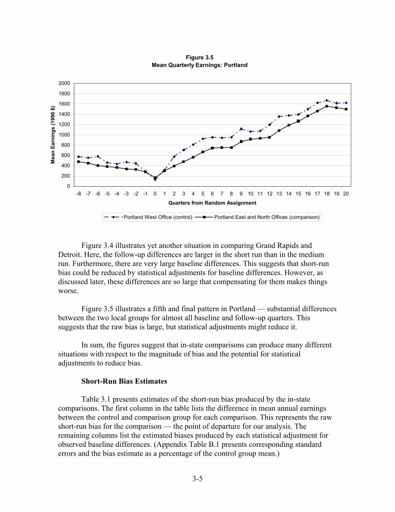
3-5

Figure 3.5Mean Quarterly Earnings: Portland

0

200

400

600

800

1000

1200

1400

1600

1800

2000

-8 -7 -6 -5 -4 -3 -2 -1 0 1 2 3 4 5 6 7 8 9 10 11 12 13 14 15 16 17 18 19 20

Quarters from Random Assignment

Mea

n Ea

rnin

gs (1

996

$)

Portland West Office (control) Portland East and North Offices (comparison)

Figure 3.4 illustrates yet another situation in comparing Grand Rapids and Detroit. Here, the follow-up differences are larger in the short run than in the medium run. Furthermore, there are very large baseline differences. This suggests that short-run bias could be reduced by statistical adjustments for baseline differences. However, as discussed later, these differences are so large that compensating for them makes things worse.

Figure 3.5 illustrates a fifth and final pattern in Portland — substantial differences between the two local groups for almost all baseline and follow-up quarters. This suggests that the raw bias is large, but statistical adjustments might reduce it. In sum, the figures suggest that in-state comparisons can produce many different situations with respect to the magnitude of bias and the potential for statistical adjustments to reduce bias. Short-Run Bias Estimates Table 3.1 presents estimates of the short-run bias produced by the in-state comparisons. The first column in the table lists the difference in mean annual earnings between the control and comparison group for each comparison. This represents the raw short-run bias for the comparison — the point of departure for our analysis. The remaining columns list the estimated biases produced by each statistical adjustment for observed baseline differences. (Appendix Table B.1 presents corresponding standard errors and the bias estimate as a percentage of the control group mean.)

3-6

Oklahoma City Rural/Oklahoma City Central -147 -30 -27 -165 35 138 -20 -153 -63

Detroit Fullerton/ Detroit Hamtramck 73 -65 -59 -169 -149 -44 -91 -155 -82

Riverside City/ Riverside County -93 -275 * -313 * -242 -475 *** -109 -443 ** -217 -332 **

Grand Rapids/ Detroit 444 *** -168 11 168 -167 -665 *** 98 141 82Portland West/

Portland East and North 765 *** 652 *** 763 *** 424 535 ** 994 ** 686 ** 340 637 ***

Mean Bias 208 23 75 3 -44 63 46 -9 48Mean Percent Bias 7 -1 1 -2 -3 1 0 -2 0Mean Absolute Bias 304 238 235 234 272 390 268 201 239Mean Percent Absolute Bias 12 9 9 10 11 15 10 8 9Percent of Estimates that are

Statistically Significant 40 40 40 0 40 40 40 0 40

Notes: Short run is defined as the two years following random assignment. Two-tailed t-tests were applied to estimates of bias.Statistical significance levels are indicated as: * = 10 percent; ** = 5 percent; *** = 1 percent. All dollar amounts are in 1996 dollars.Control group average annual earnings are $1,742 in Oklahoma City, $2,080 in Detroit, $2,289 in Riverside, $2,484 in Grand Rapids, and $3,096 in Portland.

Table 3.1

Estimated Short-Run Bias for In-State Comparisons

Fixed-effects

with one-to-one

matching

Propensity score

weighted regression

Fixed-effects model

Random-growth model

Propensity score one-to-

one matching

Propensity score sub-

classificationOLS

regressionControl Group Site / Comparison Group Site

Difference of means

Fixed-effects with sub-

classification matching

3-7

For Differences of Means

Consistent with Figures 3.1 through 3.5, there is substantial variation in the inherent short-run bias of the five comparisons. For Oklahoma City, Detroit, and Riverside, the magnitude of the estimated bias was less than $150 per year and was not statistically significant. For the other two comparisons, the bias was statistically significant and much larger — $444 for Grand Rapids-Detroit and $765 for Portland.

The bottom panel in the table presents several alternative measures that summarize the bias estimates in the top panel: the mean bias, in dollars per year and as a percent of control group earnings; the mean absolute bias, in dollars per year and as a percent of control group earnings; and the percentage of bias estimates that were statistically significant at the 0.10 level (for a two-tailed test).

For multi-site evaluations, where the main focus is on average impacts across

sites, the mean bias may be an important consideration. The mean bias using the difference of means was $208 per year or 7 percent of control group earnings.

For some studies, an evaluator might be interested in the effect of a program at a

single site. For such evaluations, a small mean bias provides cold comfort if it represents large offsetting positive and negative biases. In this case, the mean absolute bias, which represents the expected magnitude of bias for a single impact estimate, is a better guide to the suitability of an estimator. The mean absolute bias using the difference of means in Table 3.1 was $304 per year or 12 percent of control group earnings.

Are these estimated biases large? One way to judge them is by whether they are

statistically significantly different from zero. Table 3.1 indicates that two out of five differences of means, or 40 percent, are statistically significant.

Another way to assess the findings is to compare them to the original NEWWS

impact estimates. For example, the widely acclaimed Portland program studied in NEWWS increased average annual earnings by $921 during the first two years after random assignment.2 The Labor Force Attachment (LFA) programs in Atlanta, Grand Rapids, and Riverside increased average annual earnings by $406 to $638. Education-focused programs in six sites studied in NEWWS increased annual average earnings by $158 to $290. Hence, the NEWWS researchers concluded, “One program — the Portland (Oregon) one — by far outperformed the other 10 programs in terms of employment and earnings gains as well as providing a return on every dollar the government invested in the program” (Hamilton, et al., 2001, page ES-3). Further, employment-focused programs produced larger gains in employment and earnings over the two-year follow-up period than education-focused programs (Freedman, et al., 2000, page ES-15). 2 Two-year impacts are taken from Freedman, et al., 2000, Exhibit ES-5. Results in Freedman, et al., 2000, were presented in nominal (i.e., not inflation-adjusted) dollars and are therefore not directly comparable to results in Table 3.1. Because inflation was low during the 1990s, however, adjusting for inflation is unlikely to make a substantial difference in this comparison.

3-8

Would the biases in Table 3.1 have changed these conclusions? The average bias using the difference of means ($208) would have reduced, but would not have eliminated, the gap among the three approaches. Still, if the job-search-first programs had effects ranging as high as $846 per year (the largest estimate of $638 + the average bias of $208), Portland’s program would not have looked so clearly superior to job search. Likewise, a bias of $208 would have nearly eliminated the gap between the job search and education approaches. Although the average bias might not have changed the original NEWWS conclusions, the largest bias ($765 for Portland) would have overwhelmed the differences among programs and perhaps caused the original study to reach different conclusions. Chapter 4 addresses this issue more systematically.

Another way to judge whether nonexperimental estimation biases are large is to

compare them to observed baseline differences between experimental program and control groups. Although such experimental baseline differences should be zero, on average, their actual values vary across studies due to random sampling error. In 21 experimental studies of welfare and work programs conducted by MDRC during the past decade, the average annual baseline earnings difference was $21 in 1996 dollars. This is much smaller than the average difference of means in Table 3.1.3 The mean absolute baseline difference for the 21 studies was $162, or just over half of its counterpart in Table 3.1. A handful of the random assignment studies had much larger baseline differences, with the most extreme being $571. This is larger than four of the five bias estimates in Table 3.1 for a difference of means.

Lastly note that specification tests recommended by Heckman and Hotz (1989)

(discussed earlier) to eliminate inappropriate nonexperimental estimators would suggest not using comparison groups with statistically significant baseline differences. Among the five in-state comparisons, only the comparison between Grand Rapids and Detroit had a significant difference prior to random assignment. The mean absolute bias of the remaining four comparisons was $216, which is close to that for the random assignment baseline differences.

With Statistical Adjustments Table 3.1 shows that the eight nonexperimental adjustments did not reduce short-

run bias appreciably. For example, they made little difference for Oklahoma City and Detroit because baseline earnings differences between the control and comparison groups were small in those comparisons (as suggested earlier by Figures 3.1 and 3.2). Fortunately, these adjustments were not needed because the raw bias was small to begin with.

3 The 21 programs include the nine NEWWS programs in the six sites discussed in this report; six counties studied in the evaluation of the California GAIN program (Riccio, Friedlander, and Freedman, 1994), two versions of the Vermont Welfare Restructuring Project (Bloom, Michalopoulos, Walter, and Auspos, 1998), the Florida Family Transition Project (Bloom, et al., 2000a), Connecticut’s Jobs First program (Bloom, et al., 2000b) and two versions of the Minnesota Family Investment Program (Miller, et al., 2000).

3-9

Figures 3.3 through 3.5 suggested that statistical adjustments might be better able to reduce bias for the other three in-state comparisons because their baseline earnings differences were larger. Results for these comparisons varied considerably, however. For Riverside, adjustments produced a larger bias than the difference of means. For the comparison between Grand Rapids and Detroit, most of the adjustments produced a smaller bias than the difference of means, but one (the random-growth model) produced a larger bias. For Portland, most adjustments produced bias estimates that were similar to the difference of means.

There is also little evidence in Table 3.1 that any of the adjustment methods

outperformed the others consistently or appreciably. The mean bias for these methods ranged from - $9 for a fixed-effects model combined with one-to-one matching to $75 for propensity score sub-classification. The mean absolute bias ranged from $201 for a fixed-effects model combined with one-to-one matching to $390 for a random-growth model.

Our finding that statistical adjustments do not markedly reduce bias for nonexperimental comparisons is different from findings of previous research based on voluntary training programs such as National Supported Work and JTPA (LaLonde, 1986; Dehejia and Wahba, 1999; and Heckman, Ichimura, and Todd, 1997).

Medium-Run Bias Estimates Table 3.2 presents medium-run bias estimates for the in-state comparisons. (Appendix Table B.2 reports corresponding standard errors and the bias estimate as a percentage of the control group mean.) Consider the raw bias for a difference of means. The distribution of unadjusted medium-run biases is similar to its short-run counterpart. When statistical adjustments are used, the mean and mean absolute biases are typically larger in the medium run than in the short run. However, reflecting the fact that average earnings in the medium run are also higher, the mean percent bias in the medium run is similar to the short run, and the mean percent absolute bias is just slightly higher.

Lastly note that although medium-run bias estimates are often large, their mean is usually close to zero, ranging from -$228 for a fixed-effects model to $151 for a difference of means. This suggests that large positive medium-run biases are offsetting large negative ones, as was the case for short-run bias.

3-10

Oklahoma City Rural/Oklahoma City Central 84 280 305 * 380 332 * 549 274 395 202

Detroit Fullerton/ Detroit Hamtramck -590 * -913 *** -768 ** -1450 *** -973 *** -752 -843 ** -1476 *** -894 ***

Riverside City/ Riverside County 574 ** 367 346 515 * 158 931 254 526 * 322

Grand Rapids/ Detroit 24 -1164 *** -968 ** -745 -1154 *** -2206 *** -902 ** -751 -895 ***Portland West/

Portland East and North 662 634 755 * 353 496 1464 * 553 244 647 *

Mean Bias 151 -159 -66 -189 -228 -3 -133 -212 -124Mean Percent Bias 3 -2 0 -2 -3 2 -2 -3 -2Mean Absolute Bias 387 671 628 689 623 1180 565 679 592Mean Percent Absolute Bias 8 14 13 15 13 24 12 15 12Percent of Estimates that are

Statistically Significant 40 40 80 40 60 40 40 40 60

Notes: Medium run is defined as the third through fifth years following random assignment. Two-tailed t-tests were applied to estimates of bias.Statistical significance levels are indicated as: * = 10 percent; ** = 5 percent; *** = 1 percent. All dollar amounts are in 1996 dollars.Control group average annual earnings are $3,164 in Oklahoma City, $5,042 in Detroit, $4,100 in Riverside, $5,392 in Grand Rapids, and $5,538 in Portland.

Fixed-effects with sub-

classification matching

Table 3.2

Estimated Medium-Run Bias for In-State Comparisons

Fixed-effects

with one-to-one

matching

Propensity score

weighted regression

Fixed-effects model

Random-growth model

Propensity score one-to-

one matching

Propensity score sub-

classificationControl Group Site / Comparison Group Site

OLS regression

Difference of means

3-11

Adding a Third Year of Baseline History The previous sections indicate that adjusting for observed background characteristics and two years of baseline employment and earnings histories did not substantially reduce the short-run or medium-run bias produced by nonexperimental comparison groups. This section explores whether having an additional year of baseline history alters the conclusion. Fortunately, the subsamples with three years of baseline history were large enough to address this question for four of the five in-state comparisons — all except Portland. To do so, the preceding analyses were conducted twice for these subsamples — once using all three years of baseline history and again using only the two most recent years.4 If the third year of information were important, the estimated bias would be smaller when it was used. Table 3.3 presents these findings for short-run bias. The top panel in the table presents findings for three years of baseline history (12 quarters) and the bottom panel presents findings for two years (eight quarters). Note that results for the difference of means are identical in the two panels because they do not adjust for baseline histories. All of the other methods adjust for these histories, as well as for demographic characteristics. As can be seen, adding a third year of baseline history does not usually make much difference, although it did result in about one-sixth to one-fourth less mean absolute bias for two of the adjustments (fixed-effects and propensity score one-to-one matching, respectively). Table 3.4 reports corresponding findings for medium-run bias. Adding a third baseline year makes more of a difference for this follow-up period, although most estimates of bias in the medium run are still quite large. Therefore, it appears that having three years of baseline earnings history for in-state comparisons reduces bias somewhat in the medium run, but not much in the short-run. On balance, however, it does not change our conclusions. Out-of-State Comparisons This section presents findings for the 14 out-of-state comparison groups. As noted earlier, prior research by Friedlander and Robins (1995) and Heckman, Ichimura, and Todd (1997) suggests that out-of-state comparison groups should perform less well than in-state comparisons. Nevertheless, statistical adjustments for the likely larger baseline differences for out-of-state comparison groups might improve their relative performance.

4 The models with two years of baseline data were re-estimated because the subsamples with three years of prior earnings data were smaller than the full samples with two years of data used in Tables 3.1 and 3.2 for all comparisons except the comparison within Detroit.

3-12

Oklahoma City/ Oklahoma City -110 -40 123 140 42 94 64 170 -47Detroit / Detroit 73 -75 -93 50 -161 94 -173 59 -69Riverside / Riverside 78 -191 -257 -224 -348 * -267 -411 * -138 -275Grand Rapids/ Detroit 657 *** -75 120 36 -45 -609 ** 384 224 271 *

Mean Bias 175 -95 -27 1 -128 -172 -34 79 -30Mean Absolute Bias 229 95 148 113 149 266 258 148 166Percent of Estimates that are

Statistically Significant 25 0 0 0 25 25 25 0 25

Oklahoma City/ Oklahoma City -110 -41 35 -76 45 44 44 -104 -42Detroit / Detroit 73 -65 -59 -169 -149 -44 -91 -155 -82Riverside / Riverside 78 -172 -305 -249 -364 * -150 -435 ** -257 -260Grand Rapids/ Detroit 657 *** -56 219 143 -141 -545 * 358 102 302 **

Mean Bias 175 -83 -28 -87 -152 -174 -31 -104 -21Mean Absolute Bias 229 83 155 159 175 196 232 155 172Percent of Estimates that are

Statistically Significant 25 0 0 0 25 25 25 0 25

Notes: Short run is defined as the two years following random assignment. All dollar amounts are in 1996 dollars.Two-tailed t-tests were applied to estimated bias. Statistical significance levels are indicated as: * = 10 percent; ** = 5 percent; *** = 1 percent.

Control Group Site / Comparison Group Site

Random- growth model

Fixed-effects with sub-

classification matching

Fixed-effects model

Propensity score weighted

regression

Fixed-effects with one-to-

one matching

Propensity score sub-

classification

Difference of means

OLS regression

Difference of means

OLS regression

Propensity score sub-

classification

Using 8 Quarters of Prior Earnings and Employment Information

Propensity score one-to-one matching

Table 3.3

Using 12 Quarters of Prior Earnings and Employment Information

Propensity score one-to-one matching

Propensity score weighted

regression

Fixed-effects with one-to-

one matching

Fixed-effects with sub-

classification matching

Fixed-effects model

Sensitivity of Estimated Short-Run Bias for In-State Comparisons to Amount of Earnings History

Random- growth model

Control Group Site / Comparison Group Site

3-13

Oklahoma City/ Oklahoma City 326 433 * 463 90 518 ** 618 429 187 358 ***Detroit / Detroit -590 * -940 *** -836 ** -856 * -1000 *** -869 * -897 *** -856 * -877 ***Riverside / Riverside 768 *** 470 * 250 376 347 501 159 395 353Grand Rapids/ Detroit 248 -1043 *** -477 -863 -1000 *** -2077 *** -877 -916 -776 ***

Mean Bias 188 -270 -150 -313 -284 -456 -297 -297 -236Mean Absolute Bias 483 722 507 547 716 1016 591 589 591Percent of Estimates that are

Statistically Significant 50 100 25 25 75 50 25 25 75

Oklahoma City/ Oklahoma City 326 437 * 516 * 288 515 ** 514 558 ** 225 390 *Detroit / Detroit -590 * -913 *** -768 -1450 *** -973 *** -752 -843 ** -1476 *** -894 ***Riverside / Riverside 768 *** 530 ** 347 ** 355 320 772 245 401 397Grand Rapids/ Detroit 248 -1010 *** -997 ** -1016 * -1076 *** -1929 *** -769 -1099 ** -710 ***248Mean Bias 188 -239 -225 -456 -304 -349 -202 -487 -204Mean Absolute Bias 483 722 657 777 721 992 604 800 598Percent of Estimates that are

Statistically Significant 50 100 75 50 75 25 50 50 75

Notes: Medium run is defined as the third through fifth years following random assignment. All dollar amounts are in 1996 dollars.Two-tailed t-tests were applied to estimated bias. Statistical significance levels are indicated as: * = 10 percent; ** = 5 percent; *** = 1 percent.

Table 3.4

Using 12 Quarters of Prior Earnings and Employment Information

Propensity score one-to-one matching

Propensity score weighted

regression

Fixed-effects with one-to-

one matching

Fixed-effects with sub-

classification matching

Fixed-effects model

Sensitivity of Estimated Medium-Run Bias for In-State Comparisons to Amount of Earnings History

Random-growth model

Control Group Site / Comparison Group Site

Propensity score sub-

classification

Using 8 Quarters of Prior Earnings and Employment Information

Propensity score one-to-one matching

Fixed-effects with sub-

classification matching

Fixed-effects model

Control Group Site / Comparison Group Site

Difference of means

OLS regression

Difference of means

OLS regression

Random-growth model

Propensity score weighted

regression

Fixed-effects with one-to-

one matching

Propensity score sub-

classification

3-14

A First Look at the Situation Figure 3.6, which compares earnings for control group members from the six NEWWS sites, provides a first indication of the likely bias created by using individuals from a site in one state as a comparison group for a site in another state. The figure also provides initial clues about the likelihood that statistical adjustments will reduce this bias.

Figure 3.6Average Quarterly Earnings by Site

0

200

400

600

800

1000

1200

1400

1600

1800

2000

-8 -7 -6 -5 -4 -3 -2 -1 0 1 2 3 4 5 6 7 8 9 10 11 12 13 14 15 16 17 18 19 20

Quarters from Random Assignment

Mea

n Ea

rnin

gs (1

996

$)

Riverside Portland Detroit Grand Rapids Atlanta Oklahoma City

As can be seen, earnings differences were quite large across sites throughout much of the baseline period. These differences may mean that statistical adjustments can reduce bias substantially. On the other hand, they may reflect the existence of few similar individuals across sites, which would make matching quite difficult. In five of the six sites, baseline earnings declined precipitously as sample members approached their quarter of random assignment. Nearly all of these sample members were receiving welfare benefits at random assignment and many had recently begun to do so. Hence, the observed earnings decline probably reflects the rate at which sample members became unemployed and went on welfare prior to random assignment. The one exception to this pattern was in Oklahoma City, where average baseline earnings increased just before random assignment and temporarily decreased immediately thereafter. Most Oklahoma City sample members were randomly assigned when they applied for welfare, which was not the case elsewhere. This difference in the point of random assignment, and its potential reflection in baseline earnings, suggest that it may be difficult to find good matches for Oklahoma City.

3-15

Lastly note that average earnings differed relatively little during the early part of the follow-up period. This suggests that the short-run bias is probably small for many of the cross-state comparisons. However, average earnings diverged thereafter into two clusters of sites. This suggests that the medium-run bias is probably larger for comparisons across clusters than within them.

The Findings As noted earlier, 14 unique out-of-state comparisons were constructed, as follows,

using the six NEWWS sites in our analysis. A first control site (Riverside) was chosen at random from the initial six, and the other five were used as comparison groups for it. A second control site (Portland) was chosen at random from the remaining five sites, and the other four sites were used as comparison groups for it. This process continued until 15 comparisons had been identified. One of these comparisons, Detroit-Grand Rapids, was eliminated because it was one of our in-state comparisons.

Tables 3.5 and 3.6 present estimates of the biases produced by each of the 14 out-

of-state comparisons, in the short run and medium run, and with and without statistical adjustments. (Appendix Tables B.3 and B.4 present corresponding standard errors and the bias estimate as a percentage of the control group mean). Tables 3.7 and 3.8 summarize these many different findings to help paint an overall picture.

The most striking site-specific findings were for comparisons involving

Oklahoma City, which produced especially large biases in both the short run and medium run. In addition, it was not possible to balance propensity scores for any cross-state comparison that involved Oklahoma City, eliminating these comparisons from further consideration for any method involving estimated propensity scores. Furthermore, statistical adjustments that were applied to the full comparison samples for Oklahoma City (those not using propensity score matching or sub-classification) did not reduce bias appreciably or consistently.

As noted, Tables 3.7 and 3.8 summarize the out-of-state comparisons. The summary statistics presented include all of those used for the in-state comparisons plus two new ones: (1) the distribution of absolute percent bias estimates, and (2) the total number of comparisons made for a specific estimation method. The second indicator was included to highlight the fact that not all 14 comparisons were made for propensity score methods because balance could not be achieved for some comparisons.

3-16

RiversidePortland -181 -646 *** -740 *** -549 * -1100 *** -1220 *** -821 *** -375 -693 ***Detroit 296 ** -422 ** 294 -17 -755 *** -904 *** 27 -112 19Grand Rapids -148 -518 *** -466 ** -441 -1018 *** -608 ** -541 ** -219 -307 **Atlanta -344 ** -828 *** -860 * -693 -1075 *** -1693 *** -744 -334 -578 ***Oklahoma City 478 *** 230 ** NB NB -250 ** 513 *** NB NB NB

Mean Bias 20 -437 -443 -425 -840 -783 -520 -260 -390Mean Percent Bias 1 -19 -19 -18 -36 -34 -22 -11 -17Mean Absolute Bias 289 529 590 425 840 988 533 260 399Mean Absolute Percent Bias 12 23 25 18 36 42 23 11 17Percent of Estimates that are Statistically Significant 60 100 75 25 100 100 50 0 75

PortlandDetroit 477 *** 306 * 433 595 * 278 311 273 497 375 ***Grand Rapids 34 160 -189 -184 197 526 * -93 -149 -67Atlanta -162 -120 -391 -540 95 -493 -76 -409 -290 **Oklahoma City 660 *** 774 *** NB NB 804 *** 1820 *** NB NB NB

Mean Bias 252 280 -49 -43 343 541 35 -20 6Mean Percent Bias 10 11 -2 -2 14 21 1 -1 0Mean Absolute Bias 333 340 338 440 343 788 147 352 244Mean Absolute Percent Bias 13 14 13 17 14 31 6 14 10Percent of Estimates that are Statistically Significant 50 50 0 33 25 50 0 0 67

(continued)

Difference of means

OLS regression

Propensity score

weighted regression

Table 3.5

Fixed-effects with sub-

classification matching

Estimated Short-Run Bias for Out-of-State Comparisons

Fixed-effects with one-to-

one matching

Propensity score sub-

classification

Propensity score one-to-one matching

Fixed-effects model

Random-growth model Control and Comparison Site

3-17

DetroitAtlanta -640 *** -204 -219 * -251 25 -579 * -140 -198 * -275 **Oklahoma City 182 ** 461 *** NB NB 594 *** 1614 *** NB NB NB

Mean Bias -229 129 309 518Mean Percent Bias -11 6 15 25Mean Absolute Bias 411 333 309 1097Mean Absolute Percent Bias 20 16 15 54Percent of Estimates that are Statistically Significant 100 50 50 100

Grand RapidsAtlanta -196 -702 *** NB NB -387 * -1779 *** NB NB NBOklahoma City 626 *** 616 *** NB NB 589 *** 1421 *** NB NB NB

Mean Bias 215 -43 101 -179Mean Percent Bias 9 -2 4 -7Mean Absolute Bias 411 659 488 1600Mean Absolute Percent Bias 17 27 20 64Percent of Estimates that are Statistically Significant 50 100 100 100

AtlantaOklahoma City 822 *** 1034 *** NB NB 806 *** 3018 *** NB NB NB

Percent Bias 31 39 30 113Absolute Bias 822 1034 806 3018

Notes: Short run is defined as the two years following random assignment. Two-tailed t-tests were applied to each estimated bias. Statistical significance levels are indicated as: * = 10 percent; ** = 5 percent; *** = 1 percent. NB indicates that the groups could not be balanced. Average annual earnings are $2,336 in Riverside, $2,517 in Portland, $2,040 in Detroit, $2,484 in Grand Rapids, $2,680 in Atlanta, and $1,858 in Oklahoma City.

Table 3.5 (Continued)

Control and Comparison SiteDifference of means

OLS regression

Propensity score sub-

classification

Propensity score one-to-one matching

Fixed-effects model

Random-growth model

Propensity score

weighted regression

Fixed-effects with sub-

classification matching

Fixed-effects with one-to-

one matching

3-18

RiversidePortland -1228 *** -1816 *** -1964 *** -1790 * -2230 *** -2484 *** -2119 *** -1604 *** -1881 ***Detroit -1560 *** -2755 *** -2099 *** -2671 -3062 *** -3377 *** -2442 *** -2923 *** -2313 ***Grand Rapids -1583 *** -2024 *** -1912 *** -1899 -2507 *** -1642 *** -2035 *** -1710 *** -1746 ***Atlanta -1086 *** -1718 *** -1152 * -810 -1966 *** -3270 *** -1094 * -325 -767 ***Oklahoma City 711 *** 285 ** NB NB -138 1473 *** NB NB NB

Mean Bias -949 -1606 -1782 -1792 -1981 -1860 -1923 -1640 -1677Mean Percent Bias -25 -42 -47 -47 -52 -49 -50 -43 -44Mean Absolute Bias 1234 1720 1782 1792 1981 2449 1923 1640 1677Mean Absolute Percent Bias 32 45 47 47 52 64 50 43 44Percent of Estimates that are Statistically Significant 100 100 100 25 80 100 100 75 100

PortlandDetroit -331 -825 ** -727 -562 -827 ** -758 -844 -730 -750 ***Grand Rapids -355 -414 -630 ** -650 * -369 326 -566 -596 -494 **Atlanta 142 274 396 509 454 -787 900 1023 565 ***Oklahoma City 1939 *** 1942 *** NB NB 1953 *** 4098 *** NB NB NB

Mean Bias 349 244 -320 -234 303 720 -170 -101 -226Mean Percent Bias 7 5 -6 -5 6 14 -3 -2 -4Mean Absolute Bias 692 864 584 574 901 1492 770 783 603Mean Absolute Percent Bias 14 17 12 11 18 30 15 16 12Percent of Estimates that are Statistically Significant 25 50 33 33 50 25 0 0 100

(continued)

Propensity score one-to-one matching

Fixed-effects model

Random-growth model Control and Comparison Site

Table 3.6

Difference of means

Fixed-effects with sub-

classification matching

Propensity score

weighted regression

OLS regression

Estimated Medium-Run Bias for Out-of-State Comparisons

Fixed-effects with one-to-

one matching

Propensity score sub-

classification

3-19

DetroitAtlanta 474 ** 977 *** 1028 *** 1044 *** 1168 *** -107 1045 1084 *** 919 ***Oklahoma City 2270 *** 2799 *** NB NB 2892 *** 5046 *** NB NB NB

Mean Bias 1372 1888 2030 2470Mean Percent Bias 26 35 38 46Mean Absolute Bias 1372 1888 2030 2576Mean Absolute Percent Bias 26 35 38 48Percent of Estimates that are Statistically Significant 100 100 100 50

Grand RapidsAtlanta 497 ** -333 NB NB -67 -3007 *** NB NB NBOklahoma City 2294 *** 2158 *** NB NB 2120 *** 3877 *** NB NB NB

Mean Bias 1396 913 1026 435Mean Percent Bias 26 17 19 8Mean Absolute Bias 1396 1245 1094 3442Mean Absolute Percent Bias 26 23 20 64Percent of Estimates that are Statistically Significant 100 50 50 100

AtlantaOklahoma City 1797 *** 2090 *** NB NB 1874 *** 6544 *** NB NB NB

Percent Bias 37 43 38 134Absolute Bias 1797 2090 1874 6544

Notes: Medium run is defined as the third through fifth years following random assignment. Two-tailed t-tests were applied to each estimated bias. Statistical significance levels are indicated as: * = 10 percent; ** = 5 percent; *** = 1 percent. NB indicates that the groups could not be balanced. Average annual earnings are $3,809 in Riverside, $5,037 in Portland, $5,369 in Detroit, $5,392 in Grand Rapids, $4,895 in Atlanta, and $3,098 in Oklahoma City.

Table 3.6 (Continued)

Control and Comparison SiteDifference of means

OLS regression

Propensity score sub-

classification

Propensity score one-to-one matching

Fixed-effects model

Random-growth model

Fixed-effects with sub-

classification matching

Fixed-effects with one-to-

one matching

Propensity score

weighted regression

3-20

Mean bias 136 10 -267 -260 -86 139 -264 -162 -227Mean percent bias 5 0 -12 -11 -4 5 -11 -7 -10Mean absolute bias 375 501 449 409 569 1179 339 287 325Mean absolute percent bias 16 21 19 17 24 49 14 12 14Absolute bias as percent of control

group mean (% in each category)Less than 10.0 43 29 13 25 21 0 50 50 2510.0 -24.9 29 36 63 63 29 29 25 50 6325.0 or above 29 36 25 13 50 71 25 0 13

Percent of biases that are statistically significant (%) 64 79 50 25 71 86 25 13 75

Number of tests 14 14 8 8 14 14 8 8 8

Table 3.7

Fixed-effects with sub-

classification matching

Summary Statistics for Estimated Short-Run Bias in Out-of-State Comparisons

Fixed-effects with one-to-

one matching

Propensity score sub-

classification

Propensity score one-to-one matching

Fixed-effects model

Random-growth model Descriptive Statistic

Difference of means

OLS regression

Propensity score

weighted regression

3-21

Mean bias 284 46 -883 -853 -50 424 -894 -722 -808Mean percent bias 3 -3 -23 -23 -6 4 -24 -20 -22Mean absolute bias 1162 1458 1239 1242 1545 2628 1381 1249 1179Mean absolute percent bias 25 32 30 30 35 57 33 30 29Absolute bias as percent of control

group mean (% in each category)Less than 10.0 36 29 13 0 29 14 0 13 1310.0 -24.9 7 14 38 63 14 14 50 50 5025.0 or above 57 57 50 38 57 71 50 38 38

Percent of biases that are statistically significant (%) 79 79 75 38 71 71 50 50 100

Number of tests 14 14 8 8 14 14 8 8 8

Difference of means

OLS regression

Propensity score

weighted regression

Table 3.8

Fixed-effects with sub-

classification matching

Summary Statistics for Estimated Medium-Run Bias in Out-of-State Comparisons

Fixed-effects with one-to-

one matching

Propensity score sub-

classification

Propensity score one-to-one matching

Fixed-effects model

Random-growth model Descriptive Statistic

3-22

Based on all 14 comparisons, the mean short-run bias for a difference of means was $136 per year or 5 percent of control group earnings, and the mean absolute bias was $375 per year or 16 percent of control group earnings. These compare favorably to their in-state counterparts ($208 per year or 7 percent and $304 per year or 12 percent of control group earnings, respectively). Furthermore, as was the case for in-state comparisons, statistical adjustments had little effect on the short-run results for out-of-state comparisons.

In the medium run, however, out-of-state comparison groups performed markedly

less well than their in-state alternatives. Based on all 14 comparisons, the mean absolute bias was $1162 per year or 25 percent of control group earnings. These findings are consistent with prior research cited earlier. However, the fact that statistical adjustments had very little effect, in both the medium run and short run, is not consistent with prior research. Multi-State Comparisons When evaluating a program, it is unlikely that researchers would compare outcomes for participants with those for individuals from one other state. However, past researchers have chosen comparison groups from national survey samples. Although the NEWWS data do not represent a national sample, they do make it possible to compare outcomes for persons from each site with those for individuals from the other sites (states) combined. These composite multi-state comparison groups might improve the ability of matching methods to reduce bias by providing a broader pool of sample members to choose from. Tables 3.9 and 3.10 present the estimates of the bias produced by multi-state comparison groups, in the short run and long run, and with and without statistical adjustments. The top panel of the table presents bias estimates for each comparison group and the bottom panel summarizes these findings (Appendix Tables B.5 and B.6 present corresponding standard errors and the bias estimate as a percentage of the control group mean).

For the difference of means, the magnitudes of estimated short-run and medium-

run bias in Tables 3.9 and 3.10 are comparable to those for in-state and out-of-state comparisons. However, the multi-state bias estimates were statistically significant more often because of their larger samples.

We expected multi-state comparison groups to perform especially well with

propensity score matching and sub-classification because they provide a much larger and broader pool of potential matches. Because of this, we also hoped to find an acceptable match for Oklahoma City. Neither of these expectations was realized, however. We could not achieve balance for Oklahoma City using propensity score methods and none of the other statistical adjustments markedly reduced overall bias.

3-23

Riverside 135 -150 * NB NB -641 *** -315 * NB NB NBPortland 319 *** 533 *** 466 *** 541 *** 690 *** 952 *** 551 *** 561 *** 529 ***Detroit -225 ** 225 ** 239 *** 159 301 *** 310 292 *** 187 229 ***Grand Rapids 283 ** 217 ** 183 * -56 443 *** -55 263 ** -69 183 ***Atlanta 521 *** 522 *** 510 *** 552 *** 351 *** 1700 *** 388 *** 575 *** 497 ***Oklahoma City -526 *** -700 *** NB NB -445 *** -1328 *** NB NB NB

Mean Bias 85 108 350 299 116 211 374 313 360Mean Percent Bias 2 3 14 12 4 5 15 12 15Mean Absolute Bias 335 391 350 327 479 777 374 348 360Mean Absolute Percent Bias 15 17 14 13 21 34 15 14 15Percent of Estimates that are 83 100 100 50 100 67 100 50 100

Statistically Significant

Notes: Short run is defined as the two years following random assignment. Two-tailed t-tests were applied to each estimated bias.Statistical significance levels are indicated as: * = 10 percent; ** = 5 percent; *** = 1 percent. NB indicates that the groups could not be balanced.Average annual earnings are $2,336 in Riverside, $2,517 in Portland, $2,040 in Detroit, $2,484 in Grand Rapids, $2,680 in Atlanta, and $1,858 in Oklahoma City.

Random growth model

Fixed-effects with sub-

classification matching

Fixed-effects with one-to-one matching

Table 3.9Estimated Short-Run Bias for Multi-State Comparisons

Control SiteDifference of means

Propensity score sub-

classificationOLS

regression

Propensity score one-to-

one matching

Fixed-effects model

Propensity score

weighted regression

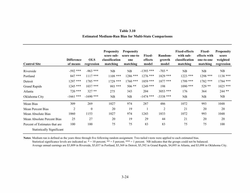
3-24

Riverside -592 *** -963 *** NB NB -1393 *** -703 * NB NB NBPortland 847 *** 1117 *** 1109 *** 1286 *** 1276 *** 1829 *** 1223 *** 1298 *** 1138 ***Detroit 1297 *** 1785 *** 1729 *** 1760 *** 1859 *** 1877 *** 1799 *** 1782 *** 1784 ***Grand Rapids 1245 *** 1037 *** 993 *** 506 ** 1249 *** 198 1090 *** 529 ** 1025 ***Atlanta 720 *** 327 ** 275 343 204 3053 *** 176 364 244 **Oklahoma City -1661 *** -1690 *** NB NB -1474 *** -3338 *** NB NB NB

Mean Bias 309 269 1027 974 287 486 1072 993 1048Mean Percent Bias 2 0 20 19 1 2 21 20 20Mean Absolute Bias 1060 1153 1027 974 1243 1833 1072 993 1048Mean Absolute Percent Bias 25 27 20 19 29 44 21 20 20Percent of Estimates that are 100 100 75 75 83 83 75 75 100

Statistically Significant

Notes: Medium run is defined as the years three through five following random assignment. Two-tailed t-tests were applied to each estimated bias.Statistical significance levels are indicated as: * = 10 percent; ** = 5 percent; *** = 1 percent. NB indicates that the groups could not be balanced.Average annual earnings are $3,809 in Riverside, $5,037 in Portland, $5,369 in Detroit, $5,392 in Grand Rapids, $4,895 in Atlanta, and $3,098 in Oklahoma City.

Table 3.10Estimated Medium-Run Bias for Multi-State Comparisons

Control SiteDifference of means

Propensity score sub-

classification matching

OLS regression

Propensity score one-to-

one matching

Propensity score

weighted regression

Fixed-effects model

Random-growth model

Fixed-effects with sub-

classification matching

Fixed-effects with one-to-one matching

3-25

Are “Site Effects” Causing the Problem? The preceding disappointing findings represent the effectiveness of a wide range

of sophisticated nonexperimental comparison group methods for an arguably “easy case” — mandatory welfare-to-work programs with participants who are similar in terms of having recently applied for or received welfare. Furthermore, the methods tested used an unusually rich set of data on individual background characteristics and labor market histories. So why did the methods perform so poorly?

One possible explanation has to do with “site effects” that could reflect

differential changes in local economic conditions.5 The estimation methods tested focus on making individual comparison group members “look” as similar as possible to their control group counterparts — by choosing samples accordingly, using statistical adjustments, or both. None of the methods, however, were designed to control for differences in local economic conditions between sites.

Changes over time in economic conditions in control and comparison counties

could account for the widely varying relationships observed for baseline and follow-up earnings. Some groups with similar earnings at baseline might have had markedly different earnings at follow-up because economic conditions in the two sites diverged. Other groups with different earnings at baseline might have had similar earnings at follow-up because their economies changed at different rates. Still other groups that had similar earnings might have remained similar over time or diverged, depending on how their respective economies performed.

As a first step toward understanding the influence of site effects on these

unpredictable situations, we compared the time path of the county unemployment rate for each of our analysis samples to the corresponding earnings path.6 In most cases, there was no clear pattern. However, the comparison of Grand Rapids and Detroit was quite intriguing and illustrates what one would look for in a potential explanation of shifting cross-site earnings relationships. Figure 3.7 illustrates these findings.

The solid line in the figure represents the difference in average quarterly earnings

between the Grand Rapids control group and the overall Detroit comparison group. During the first baseline quarter, average earnings in Grand Rapids exceeded those in Detroit by more than $300. This difference dropped to less than $100 at random assignment. It continued to decline thereafter and was negative by the end of the follow-up period — indicating that earnings in Grand Rapids had dropped slightly below those in Detroit.

5 Hollister and Hill (1995) describe the difficulties of controlling for differences in local conditions. 6 As noted in Chapter 2, random assignment dates varied within as well as across sites. We matched the relevant county quarterly unemployment rates, obtained from the U.S. Bureau of Labor Statistics, to each sample member based on her quarter of random assignment. Average quarterly unemployment rates for each site were then calculated in relation to the quarter of random assignment. This calculation corresponds with the calculation of average quarterly earnings.

3-26

Figure 3.7Difference in Earnings Compared with Difference in Unemployment Rate

Grand Rapids vs. Detroit

-300

-200

-100

0

100

200

300

400

-8 -7 -6 -5 -4 -3 -2 -1 0 1 2 3 4 5 6 7 8 9 10 11 12 13 14 15 16 17 18 19 20

Quarter from random assignment

Diff

eren

ce in

qua

rter

ly e

arni

ngs

(199

6 $)

-4

-3

-2

-1

0

1

2

Diff

eren

ce in

une

mpl

oym

ent

rate

(per

cent

age

poin

t)

earnings unemployment rate

The dashed line in the figure represents the difference each quarter between the county unemployment rate in Grand Rapids and Detroit. Its time path is nearly an exact mirror image of the time path for earnings. During the first baseline quarter, the unemployment rate in Grand Rapids was almost four percentage points lower than that in Detroit. The magnitude of this negative difference decreased to less than two points at random assignment. It continued to decrease thereafter to only one point at the end of the follow-up period.

Thus, changes in the relative unemployment rates might explain changes in the relative earnings of sample members from the two sites. Specifically, Grand Rapids’ initial earnings advantage might reflect its initially lower unemployment rate. As its unemployment advantage diminished, however, its earnings advantage also diminished at a remarkably similar rate over time.

One should not place much confidence in this explanation, however, because the

comparison between Grand Rapids and Detroit was the only one to exhibit this clear pattern. Nevertheless, given the striking, unpredictable, and different earnings changes that are experienced by groups from different locations, future research should focus more attention on the role of site effects.

4-1

Chapter 4

Summary and Conclusions

This study addresses two methodological questions in the context of evaluations of mandatory welfare-to-work programs:

• Which nonexperimental comparison group methods work best and under what conditions do they do so?

• Which, if any, of these methods produce estimates of program impacts that are

accurate enough to substitute for a random assignment experiment?

To address these questions, the study compares findings produced by a number of nonexperimental comparison group methods with those obtained from a series of random assignment experiments. This final chapter summarizes the comparisons made to help answer the questions asked. The first section of the chapter summarizes the results of different nonexperimental comparison groups and methods to determine which work best. The next section considers whether the best methods work well enough to be used instead of random assignment. The final section presents the conclusions that we believe flow from these findings.

Which Methods Work Best?

As described in the earlier chapters, biases using nonexperimental comparison groups were estimated as the differences between the counterfactuals for a series of experiments (their control group outcomes) and those predicted nonexperimentally.1 These biases were estimated for a short-run follow-up period, comprising the first two years after random assignment, and a medium-run follow-up period, comprising the third, fourth, and fifth years after random assignment.

The results in Chapter 3 indicate that biases from nonexperimental methods are positive for some applications and negative for others in ways that are not predictable. Hence, these biases tend to cancel out when averaged across many applications. The results in Chapter 3 also indicate that the positive or negative bias from a nonexperimental comparison can be quite large for a single application. Because of this, the present chapter focuses on the mean absolute bias produced by alternative methods, which represents the expected magnitudes of their biases for a given application.

Table 4.1 summarizes the mean absolute bias and the mean absolute percentage

bias of alternative estimators examined in Chapter 3 for comparisons for which baseline

1 As noted earlier, the observed differences between control group outcomes and their nonexperimental predictions represent the biases that would have been produced if the nonexperimental methods had been used to estimate program impacts.

4-2

Table 4.1 Summary of Mean Absolute Bias Estimates

for Comparisons Where Baseline Balance Was Achieved

Short-run Estimates Medium-run Estimates In-state

Comparisons (n=5)

Out-of-state Comparisons

(n=8)

Multi-state Comparisons

(n=4)

In-state Comparisons

(n=5)

Out-of-state Comparisons

(n=8)

Multi-state Comparisons

(n=4)

Mean Absolute Bias (in 1996 Dollars) Difference of means 304 285 337 387 845 1027 OLS regression 238 400 374 671 1350 1066 Propensity score sub-classification 235 449 350 628 1239 1027 Propensity score one-to-one matching 234 409 327 689 1242 974 Fixed-effect model 272 568 446 623 1573 1147 Random-growth model 390 792 754 1180 1594 1739 Fixed-effects with sub-classification 268 339 374 565 1381 1072 Fixed-effects with one-to-one matching 201 287 348 679 1249 993 Propensity score weighted regression 239 325 360 592 1179 1048 Mean Absolute Percent Bias (in Percent) Difference of means 12 12 14 8 21 20 OLS regression 9 17 15 14 33 20 Propensity score sub-classification 9 19 14 13 30 20 Propensity score one-to-one matching 10 17 13 15 30 19 Fixed-effects model 11 24 18 13 39 22 Random-growth model 15 34 30 24 40 34 Fixed-effects with sub-classification 10 14 15 12 33 21 Fixed-effects with one-to-one matching 8 12 14 15 30 20 Propensity score weighted regression 9 14 15 12 29 20 Notes: Means are calculated from the comparisons for which balance could be achieved in Tables 3.1, 3.2, 3.5, 3.6, 3.9, and 3.10.

Short-run is defined as the two years following random assignment. Medium-run is defined as the third through fifth years following random assignment.

4-3

balance was achieved using propensity score methods as a specification test.2 These findings represent the likely bias produced by program impact estimates when propensity score methods are used to screen out inappropriate comparison groups.

As noted in Chapter 3, all of the in-state comparison groups achieved balance. However, only eight of the fourteen out-of-state comparisons and four of the six multi-state comparisons did so. Thus, Table 4.2 compares bias estimates for comparisons that achieved balance with those for comparisons that did not achieve balance (using estimation approaches that do not check for balance in both cases). The first column for each time frame and type of comparison represented in the table lists findings for comparisons where balance was achieved. The second column (in parentheses) lists corresponding findings for comparisons where balance was not achieved.

Three tentative conclusions emerge from the findings reported in the two tables:

• Biases using nonexperimental comparison groups were consistently larger in the medium run than in the short run. For every combination of a comparison group and an estimation method, the mean absolute bias was larger in the medium run than in the short run. In many cases, medium-run bias was three times to five times the size of its short-run counterpart. Furthermore, the mean absolute percent bias in the medium run was larger than its short-run counterpart in all combinations except for one (difference of means). Thus, as for any prediction, it was easier to predict a counterfactual that was close in time than one that was distant in time.

• “Local” comparison groups produced the smallest mean absolute biases for

nonexperimental impact estimators. This was especially true for estimates of medium-run impacts where in-state comparison groups produced biases that generally were one-third to one-half the size of those for out-of-state and multi-state comparison groups. This finding accords with results from previous research (Friedlander and Robins, 1995; Bell, Orr, Blomquist, and Cain, 1995; and Heckman, Ichimura, and Todd, 1997). In the short run these differences were less pronounced and less consistent, but existed nonetheless.

• None of the statistical adjustment methods used to refine nonexperimental

comparison group approaches consistently reduced bias substantially. However, propensity score methods provided a specification check that tended to eliminate biases that were larger than average. Looking across the full range of impact estimation methods considered, a simple difference of means generally performed about as well as the other approaches. OLS regression, especially when used for groups that could be balanced using propensity scores, also performed relatively well compared to the more complex methods. Using a fixed-effects model, with

2 Donald Rubin noted the potential value of using propensity score balance tests to screen-out inappropriate comparison groups in his discussion at the session on “Are There Alternatives to Random Assignment?” held as part of the 2001 Fall Research Conference of the Association for Public Policy and Management.

4-4

Table 4.2 Summary of Bias Estimates for Methods that Do Not Use Propensity Scores

for Balanced and Unbalanced Comparisons Short-run Estimates Medium-run Estimates Out-of-state

Comparisons Multi-state

Comparisons Out-of-state Comparisons

Multi-state Comparisons

Balanced (n=8)

Unbalanced (n=6)

Balanced (n=4)

Unbalanced (n=2)

Balanced (n=8)

Unbalanced (n=6)

Balanced (n=4)

Unbalanced (n=2)

Mean Absolute Bias (in 1996 Dollars) Difference of means 285 (494) 337 (330) 845 (1585) 1027 (1127) OLS regression 400 (636) 374 (425) 1350 (1601) 1066 (1326) Fixed-effects model 568 (572) 446 (543) 1573 (1507) 1147 (1434) Random-growth model 792 (1694) 754 (821) 1594 (4008) 1739 (2021) Mean Absolute Percent Bias (in Percent) Difference of means 12 (20) 14 (17) 21 (31) 20 (35) OLS regression 17 (26) 15 (22) 33 (31) 20 (40) Fixed-effects model 24 (24) 18 (26) 39 (29) 22 (42) Random-growth model 34 (69) 30 (42) 40 (79) 34 (63) Notes: Short-run is defined as the two years following random assignment. Medium-run is defined as the third through fifth years following random assignment.

4-5

or without propensity score balancing, did not consistently improve the results. Using a random-growth model often increased the biases — in some cases substantially. These findings were obtained regardless of the comparison group used or the time frame of the analysis and are contrary to those from previous research (LaLonde, 1986; Fraker and Maynard, 1987; Heckman and Hotz, 1989; Heckman, Ichimura, and Todd, 1997; and Dehejia and Wahba, 1999).

Thus it appears that a local comparison group may produce the best results for the

applications that we examined and that with such comparison groups, a simple difference of means or OLS regression may perform as well or better than more complex approaches. For less proximate comparison groups, propensity score balancing methods may provide a useful specification check by eliminating problematic comparison groups from consideration. If these groups are eliminated, a simple difference of means or OLS regression can often perform as well as more complex estimators. Do The Best Methods Work Well Enough? Having established that OLS regression with an in-state comparison group (referred to hereafter as the nonexperimental estimator) is as good as or better than more complex methods, this section attempts to determine whether the approach is good enough to substitute for random assignment in evaluations of mandatory welfare-to-work programs.3 The first step in this discussion is to more fully characterize the nature and magnitude of the estimation error associated with the method. This information is then used to consider whether the method would have produced conclusions about NEWWS programs that are materially different from those obtained from the original experimental evaluations of these programs.

Nonexperimental Estimation Error Tables 3.1 and 3.2 in chapter 3 presented five short-run estimates and five medium-run estimates of the bias produced by OLS regression with an in-state comparison group. For both time periods, the mean value of the five bias estimates was close to zero (negative one percent and negative two percent of the control group mean) although the variation around the mean was substantial. This near-zero mean bias is consistent with the fact that the direction of the bias for any given application is arbitrary and in many cases would be reversed if the roles of the comparison and control groups were reversed.4 The finding is also consistent with the graphs in Figures 3.1 through 3.5 presented earlier, which indicate that knowing the baseline earnings trends for a

3 We use OLS regression as the basis for our discussion here instead of a simple difference of means (which performs as well or better) because in practice it is likely that some adjustment procedure always would be used if it were possible to do so. 4 For methods that do not use estimated propensity scores — OLS regression, fixed-effects models, and random-growth models — bias estimates will always have the same magnitudes but opposite signs depending on which group is defined as the control group and which is defined as the comparison group. However, for methods that use estimated propensity scores, it is possible that, depending upon which group provides the comparison group pool, the magnitude of the bias might differ but its sign might not.

4-6

comparison group and control group does not ensure a good prediction of how these trends will diverge, or not, in the future.

Because of this, it is appropriate in the present context to consider the theoretical sampling distribution of nonexperimental “mismatch error” across applications to have a grand mean or expected value of zero. In this regard, the error is not really a bias (which implies a non-zero expected value) but rather an additional random error component. In large part, this error component reflects unobserved “site effects” which have been very difficult to control for in past research (Hollister and Hill, 1995). The standard error of the sampling distribution of mismatch error can be inferred from the standard deviation of the five bias estimates for a given follow-up period and information about the sampling errors and sample sizes of these estimates.

With this information it is possible to assess the use of nonexperimental

comparison groups by comparing their estimated sampling distribution to that of its experimental counterpart from NEWWS. Both sampling distributions are centered on the true impact for a given analysis. The experimental estimator has one source of random error — that due to sampling a finite number of welfare recipients. Thus, its standard error reflects a single error component. The nonexperimental estimator has two sources of random error: (1) the random sampling error to which an experiment is subject, plus (2) random nonexperimental mismatch error. Thus, the standard error of the nonexperimental estimator reflects both error components and is larger than that of a corresponding experimental estimator. Although the effect of random sampling error on a single application can be reduced by increasing its sample size, the effect of nonexperimental mismatch error cannot be reduced this way (see Appendix D). This second error component can only be reduced by averaging findings across a series of applications.

The primary effect of mismatch error in the present context is thus to reduce the

statistical power of nonexperimental estimators. To compare such estimators with their experimental counterparts requires comparing their abilities to discern a specific program impact. Figure 4.1 illustrates such a comparison by showing the sampling distributions of experimental and nonexperimental impact estimators for a hypothetical true impact of $1,000. The experimental distribution is higher than the nonexperimental distribution near the true impact. This means that the experiment is more likely to produce an estimate close to truth. In contrast, the nonexperimental distribution is much lower near the true impact and much higher far away. This means that the nonexperimental estimator is less likely to produce an estimate near truth ($1,000) and more likely to produce one far away (for example, near $0 or $2,000).

The types of comparisons shown in Figure 4.1 are only possible for a

methodological study, like the present one, which can directly compare experimental and nonexperimental estimates of the same impacts. For any given application it is not possible to estimate mismatch error and account for it in the standard errors of nonexperimental impact estimates (which is clearly a problem). Having established the basic relationship between the sampling distributions for corresponding experimental and

4-7

Figure 4.1Implied Sampling Distributions of Experimental and Nonexperimental Impact Estimators for a Hypothetical Program

-1000 -500 0 500 1000 1500 2000 2500 3000

Estimated Impact on Annual Earnings

Experimental estimator Nonexperimental estimator

True Impact

4-8

nonexperimental impact estimators, it is now possible to compare their implications for specific conclusions from the original NEWWS study. The approach that we use to do so is similar in spirit to, but different in form from, that developed by Bell, Orr, Blomquist, and Cain (1995).

Implications of Nonexperimental Estimation Error Relative to the Impacts of NEWWS Programs

The NEWWS study was designed to estimate the impacts of alternative welfare-to-work strategies that had been the subject of widespread debate among policy makers, program administrators, and researchers for many years.5 The study focused on the net impacts of each programmatic approach (their impacts relative to no such special mandatory services) and their differential impacts (their impacts relative to each other). The impact findings for NEWWS were reported for four categories of programs: (1) the Portland program (which was unique relative to the others because it used a broad mix of job search and education), (2) job-search-first programs (that focused on helping clients find jobs)6, (3) high-enforcement, education-focused programs (that focused first on providing educational services and used sanctions to enforce client participation)7, and (4) low-enforcement, education-focused programs (that focused first on providing educational services but were less emphatic about client participation).8

One way to assess the importance of nonexperimental mismatch error is to

examine its implications for replicating the basic conclusions from NEWWS for these four types of programs. Table 4.3 summarizes this assessment with respect to net impacts on total earnings during the first five years after random assignment. This summary measure reflects the overall influence of estimation bias in the short and medium run.

The first two rows in Table 4.3 present the experimental point estimate and

statistical significance level (p-value) for each net program impact.9 As can be seen, the impact on total five-year follow-up earnings equals $5034 for Portland, which is statistically significant at beyond the 0.001-level. The other programs have impact estimates of $2138, $1503, and $770, all of which are statistically significant at or beyond the 0.10 level.

The experimental point estimate and its estimated standard error for each program

impact provide estimates of the corresponding expected value and standard error of the sampling distribution for that estimator. The sampling distribution for the corresponding nonexperimental estimator has the same expected value but a standard error that includes an additional component for mismatch error. One way to assess the implications of this

5 See Hamilton, et al. (2001) for a description of the NEWWS programs. 6 This category included the Labor Force Attachment programs in Atlanta, Grand Rapids, and Riverside. 7 This category included the Human Capital Development programs in Atlanta, Grand Rapids, and Riverside; and the Integrated Case Management and Traditional Case Management programs in Columbus. 8 This category included the Detroit and Oklahoma City programs. 9 Our estimates differ slightly from those presented by Hamilton, et al. (2001) because ours are reported in 1996 dollars, whereas theirs are reported in nominal dollars.

4-9

Table 4.3

Nonexperimental Estimation Error and NEWWS Net Impacts for Total Five-Year Follow-up Earnings

(1996 Dollars)

Portland

Job-search-

first

High-Enforcement Education-

Focused

Low-Enforcement Education-

Focused Experimental Impact Estimate1 Point estimate $5034 $2138 $1503 $770 Statistical significance (p-value) < 0.001 < 0.001 < 0.001 0.075 Likelihood of a significant positive experimental replication2

98% ~100% 99% 56%

Likelihood of a significant positive nonexperimental replication2

53% 39% 30% 11%

SOURCE: MDRC calculations from data collected for the National Evaluation of Welfare-to-Work Strategies. Notes: 1 The numbers of experimental and control group members per program from left to right are:(3,529 and 499), (5382 and 6292), (9716 and 8803) and (6535 and 6591). 2 Values in the table equal the probabilities (expressed as percentages) that a replication would be statistically significantly positive at the 0.05-level. The experimental standard errors from right to left are: $1327, $455, $385, $432. The corresponding nonexperimental standard errors are $2967, $1598, $1356 and $1926 (see Appendix D). mismatch error is to compare the likelihoods that, upon replication, the experimental and nonexperimental estimators would generate a second impact estimate that is statistically significantly positive at the 0.05 level. Doing so compares the likelihoods that the two estimators would replicate an important current conclusion about each program.

For Portland, the experimental estimator, with its large expected value and much smaller standard error, has a 98 percent chance of replicating a statistically significant positive impact estimate. In other words, it almost certainly would do so. In contrast, the nonexperimental estimator, with the same expected value but a much larger standard error, has only a 53 percent chance of replicating the current positive conclusion.

Even larger discrepancies exist between the experimental and nonexperimental

estimators for the next two program models in the table. In both cases, the experimental estimator is almost certain to replicate a significant positive finding, even though its expected values are only a fraction of Portland’s. This is because the experimental standard errors for these programs are much smaller than the experimental standard error

4-10

for Portland because their sample sizes are much larger (because they include several programs). Nevertheless, the corresponding nonexperimental estimators have a relatively small chance of replicating the NEWWS impact findings (39 percent and 30 percent). This is because of the large nonexperimental mismatch error whose variance does not decline with increases in the sample size at each site. The variance does decline, however, with the number of sites included for each type of program and this factor was accounted for in the analysis (see Appendix D).

Lastly, note that for the fourth program in the table, the experimental estimator,

which is statistically significant at the 0.075-level, has only a 56 percent chance of replicating a significant positive impact (its modest significance implies modest replicability). However, its nonexperimental counterpart has an even smaller chance of doing so (11 percent).

Therefore, in terms of replicating the significant positive net impact that was

observed for each of the four main types of NEWWS programs, the best nonexperimental estimator that we studied is not a good substitute for random assignment.

Now consider the findings for NEWWS differential impact estimates summarized

in Table 4.4. A differential impact estimate for two programs is simply the difference between their net impact estimates. The standard error of the difference for independent samples is the square root of the sum of the error variances for each net impact estimate. For samples that overlap, an additional covariance term is included (see Appendix D).

The top panel in the table presents the point estimates obtained for each NEWWS

differential impact. These estimates equal the differences between the net impact estimates for the programs identified in the corresponding columns and rows. Thus, for example, the Portland net impact estimate was $2896 larger than that for the job-search-first programs, $3531 larger than that for the high-enforcement education-focused programs and $4264 larger than that for the low-enforcement education focused programs. The statistical significance of each differential impact estimate is listed in its corresponding location in the second panel. As can be seen, the differential impact estimates are statistically significant at the 0.039, 0.011 and 0.002 levels, respectively. The only other significant positive differential impact estimate is for job-search-first programs versus low-enforcement education-focused programs (p=0.029).

The third panel in the table presents the likelihood that a given experimental

impact estimator would replicate a statistically significant positive impact estimate (at the 0.05-level). Thus, for the four NEWWS differential impact estimates that are significantly different from zero, this panel indicates the likelihood that the experimental estimator would replicate this basic conclusion.

Consider again the findings for Portland versus the other NEWWS programs. The

experimental estimator would have a 66 percent chance of replicating the significant positive difference between the Portland and job-search-first programs, an 82 percent chance of replicating the significant positive difference between the Portland and

4-11

Table 4.4

Nonexperimental Estimation Error and NEWWS Differential Impacts for Total Five-Year Follow-up Earnings

(1996 Dollars)

Portland Job-search-

first

High-Enforcement Education-

Focused

Low-Enforcement Education-

Focused Experimental point estimate of differential impact

Job-search-first $2896 High-enforcement education-focused $3531 $634 Low-enforcement education-focused $4264 $1368 $733 --- Experimental significance level (p-value) for differential impact estimate

Job-search-first 0.039 High-enforcement education-focused 0.011 0.575 Low-enforcement education-focused 0.002 0.029 0.205 --- Likelihood of a significant positive experimental replication1

Job-search-first 66% High-enforcement education-focused 82% 14% Low-enforcement education-focused 92% 70% 35% --- Likelihood of a significant positive nonexperimental replication1

Job-search-first 22% High-enforcement education-focused 29% 7% Low-enforcement education-focused 33% 14% 9% ---

1 Values in the table equal the probabilities (expressed as percentages) that a replication would be statistically significantly positive at the 0.05-level.

high-enforcement education-focused programs and a 92 percent chance of replicating the significant positive difference between the Portland and low-enforcement education-focused programs. In addition, the experimental estimator would have a 70 percent chance of replicating the significant positive difference between the job-search-first programs and the low-enforcement education-focused programs. Thus, experimental estimators would have reasonably good chances of replicating these important conclusions from the NEWWS experiment. In contrast, the nonexperimental estimators would have little chance of replicating any of these positive conclusions (ranging from 14 percent to 33 percent).

4-12

Thus, in terms of replicating the significant positive differential impacts that were observed for NEWWS programs, the best nonexperimental estimator that we studied is not a good substitute for random assignment.

Conclusions This study has assessed the ability of nonexperimental comparison group methods to measure the impacts of mandatory welfare-to-work programs by comparing their results to those from a series of random assignment experiments. The approaches tested included two propensity score matching methods (sub-classification and one-to-one matching), three statistical modeling methods (OLS regression, fixed-effects models, and random-growth models), plus several combinations of these methods. Tests of the approaches were based on detailed, rich, and consistent data on the background characteristics of sample members, including up to three years of quarterly baseline earnings and employment measures plus extensive socioeconomic information. Furthermore, the population used as the basis for testing — sample members from tests of mandatory welfare-to-work programs — is relatively homogenous and not subject to self-selection bias that plagues evaluations of voluntary social programs. In these regards, the conditions for the methods to perform well were favorable. The tests conducted involved multiple replications using three different types of comparison groups (in-state comparison groups, out-of-state comparison groups, and multi-state comparison groups) for two different time frames (the short run and the medium run). In addition, most tests were based on large samples. In these regards, the conditions for conducting meaningful and fair tests of the methods were favorable. So what do we conclude from these tests? With respect to the first question addressed, “which nonexperimental methods work best?” we conclude that local comparison groups are the most effective and simple differences of means or OLS regressions perform as well as more complex alternatives. Because these findings are consistent across many replications based on large samples from combinations of six different states, we believe that they probably generalize to many other mandatory welfare and work programs. It is less clear, however, how they generalize to voluntary programs where the sources, nature, and magnitude of selection bias might be different. With respect to the second question addressed, “do the best methods work well enough to replace random assignment?” we conclude that the answer is probably, “No.” The magnitude of mismatch bias for any given nonexperimental evaluation can be large, even though it varies unpredictably across evaluations with an apparent grand mean of zero. This added error component markedly reduced the likelihood that nonexperimental comparison group methods could replicate major findings from the National Evaluation of Welfare-to-Work Strategies. Perhaps even more problematic is that without random assignment it is not possible to account for mismatch error through statistical tests or confidence intervals.

4-13

Nevertheless, it is important to note two qualifications to this final conclusion. The first qualification derives from that fact that our analysis of the random variation in mismatch error is based on only five estimates of this error. A second important qualification derives from the fact that in constructing comparison groups to test, we did not fully emulate how this might be done for an actual evaluation. In practice, an evaluator would try to find local welfare offices or clusters of offices with caseloads, economic environments, and social settings that are as similar as possible to those for the local offices in which the programs are being tested. This judgmental and opportunistic office matching process was not reflected in the current analysis because: (1) more emphasis was placed on testing the different statistical methods being assessed, and (2) there were only a few combinations of local welfare offices within each site to choose from. Given the limited generalizability and verisimilitude of this part of our analysis, we believe that the jury may be still out on whether there are some important situations in which nonexperimental comparison group methods can replace random assignment to evaluate welfare-to-work programs. We therefore hope to replicate our analysis using a broader sample of random assignment studies.

R-1

References Amemiya, Takeshi (1985) Advanced Econometrics (Cambridge, MA: Harvard University

Press). Angrist, Joshua D., Guido W. Imbens, and Donald B. Rubin (1996) “Identification of

Causal Effects Using Instrumental Variables,” Journal of the American Statistical Association, Vol. 91, No. 434 (June): 444-455.

Ashenfelter, Orley (1974) “The Effect of Manpower Training on Earnings: Preliminary

Results,” (Princeton, NJ: Princeton University, Industrial Relations Section, Working Paper #60, December).

Ashenfelter, Orley (1978) “Estimating the Effects of Training Programs on Earnings,” The Review of Economics and Statistics, Vol. 60, No. 1 (February): 47-57.

Ashenfelter, Orley and David Card (1985) “Using the Longitudinal Structure of Earnings to Estimate the Effect of Training Programs,” The Review of Economics and Statistics, Vol. 67, No. 4 (November): 648-660.

Barnow, Burt S. (1987) “The Impact of CETA Programs on Earnings: A Review of the Literature,” The Journal of Human Resources, Vol. 22 (Spring): 157-193.

Barnow, Burt S., Glen G. Cain, and Arthur S. Goldberger (1980) “Issues in the Analysis of Selectivity Bias,” in Ernst Stromsdorfer and George Farkas, eds., Evaluation Studies Review Annual Volume 5 (San Francisco, CA: Sage Publications): 290-317.

Bassi, Laurie J. (1984) “Estimating the Effect of Training Programs with Non-Random Selection,” The Review of Economics and Statistics, Vol. 66, No. 1 (February): 36-43.

Bell, Stephen H., Larry L. Orr, John D. Blomquist, and Glen G. Cain (1995) Program Applicants as a Comparison Group in Evaluating Training Programs (Kalamazoo, MI: W. E. Upjohn Institute for Employment Research).

Betsey, Charles L., Robinson G. Hollister, and Mary R. Papageorgiou (1985) Youth Employment and Training Programs: The YEDPA Years. Commission on Behavioral and Social Sciences and Education, National Research Council (Washington DC: National Academy Press).

Bloom, Dan, James J. Kemple, Pamela Morris, Susan Scrivener, Nandita Verma, and Richard Hendra (2000a) The Family Transition Program: Final Report on Florida’s Initial Time-Limited Welfare Program (New York: Manpower Demonstration Research Corporation).

R-2

Bloom, Dan, Laura Melton, Charles Michalopoulos, Susan Scrivener, and Johanna Walter (2000b) Jobs First: Implementation and Early Impacts of Connecticut’s Welfare Reform Initiative (New York: Manpower Demonstration Research Corporation).

Bloom, Dan, Charles Michalopoulos, Johanna Walter, and Patricia Auspos (1998) Implementation and Early Impacts of Vermont’s Welfare Restructuring Project (New York: Manpower Demonstration Research Corporation).

Bloom, Howard S. and Maureen A. McLaughlin (1982) “CETA Training Programs-Do They Work for Adults?” (Washington, DC: U.S. Congressional Budget Office and National Commission for Employment Policy).

Bloom, Howard S., Larry L. Orr, George Cave, Stephen H. Bell, Fred Doolittle, and Winston Lin (1997) “The Benefits and Costs of JTPA Programs: Key Findings from the National JTPA Study,” The Journal of Human Resources, Vol. 32, No. 3 (Summer): 549-76.

Campbell, Donald T. and Julian C. Stanley (1963) Experimental and Quasi-experimental Design for Research (Chicago: Rand McNally and Company).

Cook, Thomas D. and Donald T. Campbell (1979) Quasi-Experimentation: Design and Analysis Issues for Field Settings (Chicago: Rand McNally College Publishing Company).

Cooley, Thomas, Thomas McGuire, and Edward Prescott (1979) “Earnings and Employment Dynamics of Manpower Trainees: An Exploratory Econometric Analysis,” in Ronald Ehrenberg, ed., Research in Labor Economics Vol. 4, Supplement 2: 119-147.

Dehejia, Rajeev H. and Sadek Wahba (1999) “Causal Effects in Nonexperimental Studies: Reevaluating the Evaluation of Training Programs,” Journal of the American Statistical Association, Vol. 94, No. 448 (December): 1053-1062.

Dehejia, Rajeev H. and Sadek Wahba (2002) “Propensity Score Matching Methods for Nonexperimental Causal Studies,” Review of Economics and Statistics, Vol. 84, No. 1 (February): 151-161.

Economic Report of the President (2000) (Washington: U.S. Government Printing Office).

Fraker, Thomas M. and Rebecca A. Maynard (1987) “The Adequacy of Comparison Group Designs for Evaluations of Employment Related Programs,” The Journal Of Human Resources, Vol. 22, No. 2 (Spring): 194-227.

R-3

Freedman, Stephen, Daniel Friedlander, Gayle Hamilton, JoAnn Rock, Marisa Mitchell, Jodi Nudelman, Amanda Schweder, and Laura Storto (2000) Evaluating Alternative Welfare-to-Work Approaches: Two-Year Impacts for Eleven Programs (Washington, DC: U.S. Department of Health and Human Services, Administration for Children and Families and Office of the Assistant Secretary for Planning and Evaluation; and U.S. Department of Education, Office of the Under Secretary and Office of Vocational and Adult Education).

Friedlander, Daniel and Philip K. Robins (1995) “Evaluating Program Evaluations: New Evidence on Commonly Used Nonexperimental Methods,” The American Economic Review, Vol. 85, No. 4 (September): 923-937

Glass, Gene V. (1976) “Primary, Secondary, and Meta-analysis of Research,” Educational Researcher, Vol. 5: 3-8.

Goldstein, Jon (1972) The Effectiveness of Manpower Training Programs: A Review of Research on the Impact of the Poor (Washington, DC: U.S. Government Printing Office).

Hamilton, Gayle and Thomas Brock (1994) The JOBS Evaluation: Early Lessons from Seven Sites. (Washington DC: U.S. Department of Health and Human Services, Administration for Children and Families, Office of the Assistant Secretary for Planning and Evaluation and U.S. Department of Education, Office of the Under Secretary, Office of Vocational and Adult Education).

Hamilton, Gayle, Stephen Freedman, Lisa Gennetian, Charles Michalopoulos, Johanna Walter, Diana Adams-Ciardullo, Ann Gassman-Pines, Sharon McGroder, Martha Zaslow, Jennifer Brooks, Surjeet Ahluwalia (2001) National Evaluation of Welfare-to-Work Strategies: How Effective Are Different Welfare-to-Work Approaches? Five-Year Adult and Child Impacts for Eleven Programs (Washington DC: U.S. Department of Health and Human Services, Administration for Children and Families, Office of the Assistant Secretary for Planning and Evaluation and U.S. Department of Education, Office of the Under Secretary, Office of Vocational and Adult Education).

Heckman, James J. (1976) “The Common Structure of Statistical Models of Truncation, Sample Selection and Limited Dependent Variables and a Simple Estimator for Such Models,” Annals of Economic and Social Measurement, Vol. 5: 475-92.

Heckman, James J. (1978) “Dummy Endogenous Variables in A Simultaneous Equation System,” Econometrica, Vol. 46: 931-59.

Heckman, James H. and V. Joseph Hotz (1989) “Choosing Among Alternative Nonexperimental Methods for Estimating the Impact of Social Programs: The Case of Manpower Training,” Journal of the American Statistical Association, Vol. 84, No. 408 (December): 862-74.

R-4

Heckman, James, Hidehiko Ichimura, Jeffrey Smith, and Petra Todd (1998) “Characterizing Selection Bias Using Experimental Data,” Econometrica, Vol. 66, No. 5: 1017-1098.

Heckman, James, Hidehiko Ichimura, and Petra Todd (1997) “Matching as An Econometric Evaluation Estimator: Evidence from Evaluating a Job Training Program,” Review of Economic Studies, Vol. 64, No. 4: 605-654.

Heckman, James, Hidehiko Ichimura, and Petra Todd (1998) “Matching as An Econometric Evaluation Estimator,” Review of Economic Studies, Vol. 65, No. 2: 261-294.

Heinsman, Donna T. and William R. Shadish (1996) “Assignment Methods in Experimentation: When Do Nonrandomized Experiments Approximate Answers From Randomized Experiments?” Psychological Methods, Vol. 1, No. 2: 154-169.

Hirano, Keisuke, Guido W. Imbens, and Geert Ridder (2000) “Efficient Estimation of Average Treatment Effects Using the Estimated Propensity Score” (Cambridge, MA: National Bureau of Economic Research, NBER Working Paper # T0251).

Hollister, Robinson G. and Jennifer Hill (1995) “Problems in the Evaluation of Community-Wide Initiatives,” in James P. Connell, Anne C. Kubisch, Lisbeth B. Schorr, and Carol H. Weiss, eds. New Approaches to Evaluating Community Initiatives: Concepts, Methods, and Contexts (Washington, DC: Aspen Institute): 127-172.

Hotz, V. Joseph, Guido W. Imbens, and Jacob A. Klerman (2000) “The Long-Term Gains from GAIN: A Re-Analysis of the Impacts of the California GAIN Program” (Cambridge, MA: National Bureau of Economic Research, November).

Hsiao, Cheng (1990) Analysis of Panel Data (Cambridge: Cambridge University Press).

LaLonde, Robert J. (1986) “Evaluating the Econometric Evaluations of Training Programs with Experimental Data,” The American Economic Review, Vol. 76, No. 4 (September): 604-620.

Lipsey, Mark W. and David B. Wilson (1993) “The Efficacy of Psychological, Educational, and Behavioral Treatment,” American Psychologist, Vol. 48, No. 12: 1181-1209.

Maddala G. S. and Lung-Fei Lee (1976) “Recursive Models with Qualitative Endogenous Variables,” Annals of Economic and Social Measurement Vol. 5: 525-45.

Miller, Cynthia, Virginia Knox, Lisa A. Gennetian, Martey Dodoo, Jo Anna Hunter, and Cindy Redcross (2000) Reforming Welfare and Rewarding Work: Final Report on the Minnesota Family Investment Program (New York: Manpower Demonstration Research Corporation).

R-5

Raudenbush, Stephen and Anthony Bryk (2002) Hierarchical Linear Models: Applications and Data Analysis, 2nd Edition (Thousand Oaks, CA: Sage Publications).

Riccio, James, Daniel Friedlander, and Stephen Freedman (1994) GAIN: Benefits, Costs, and Three-Year Impacts of a Welfare-to-Work Program (New York: Manpower Demonstration Research Corporation).

Rosenbaum, Paul R. and Donald B. Rubin (1983) “The Central Role of the Propensity Score in Observational Studies for Causal Effects,” Biometrika, Vol. 70, No. 1: 41-55.

Shadish, William R., Thomas D. Cook, and Donald T. Campbell (2002) Experimental and Quasi-experimental Designs for Generalized Causal Inference (Boston: Houghton Mifflin Company).

Smith, Jeffrey and Petra Todd (Forthcoming) “Does Matching Overcome LaLonde’s Critique of Nonexperimental Estimators?” The Journal of Econometrics.

Smith, Mary Lee, Gene V. Glass, and Thomas I. Miller (1980) The Benefits of Psychotherapy (Baltimore, MD: Johns Hopkins University Press).

Stromsdorfer, Ernst, Howard Bloom, Robert Boruch, Michael Borus, Judith Gueron, Alan Gustman, Peter Rossi, Fritz Scheuren, Marshall Smith, and Frank Stafford (1985) “Recommendations of the Job Training Longitudinal Survey Research Advisory Panel,” (Washington, DC: U.S. Department of Labor, November).

Zhao, Zhong (2000) “Using Matching to Estimate Treatment Effects: Data Requirements, Sensitivity, and an Application.” (Johns Hopkins University).

A-1

Appendix A

Derivation of Standard Errors for the Propensity Score One-to-One Matching Method and

Derivation of the Random-Growth Model

A-2

Derivation of Standard Errors for the Propensity Score One-to-One Matching Method This section of the appendix derives the formula for calculating the variances of bias estimates from one-to-one matching. Matching with replacement, the estimated bias can be written as

∑=

−=n

iii yy

nm

101 )(1

where i = 1, …, n indicates the control group member; n is the number of control group members; yi1 indicates the outcome for that control group member; and yi0 indicates the outcome for the comparison group member to whom she is matched. This expression can be rewritten as

∑∑==

−=m

jjj

n

ii yk

ny

nm

10

11

11

Here, the second sum includes an entry for each comparison group member, whether or not she was matched to a control group member, and m denotes the number of comparison group members in the full sample. The number of times the jth comparison group member is used is indicated by kj. At one extreme, each comparison group member would be matched at most once to a control group member, in which case kj = 1 for each comparison group member who is matched to a control group member. At the other extreme, one comparison group member would be matched to all control group members. In that case, kj = n for that comparison group member and kj = 0 for all other comparison group members. Note that the kj add to n. Assume that the y’s are independent across people and that a priori they come from identical distributions. We have no reason to doubt these assumptions in the current context. Then

∑∑==

+=m

jjj

n

ii yk

nVary

nVarmVar

10

11 )1()1()(

∑=

+=m

jjji yVark

nyVar

n 10

221 )(1)(1

∑=

+=m

jjk

ns

ns

1

22

20

21

where s1

2 is the estimated variance of the outcome among control group members and s02

is the estimated variance of the outcome among matched comparison group members. The use of regression adjustment results in an analogous expression, except that the variance of individual residuals from the regression is used instead of the variance of individual outcomes.

A-3

To implement the correction, we noted that the estimated variance of the bias produced by OLS is computed as follows, given that OLS assumes that the residuals for the control and comparison groups come from a common distribution with a common variance:

ns

ns

ns 222 2=+

Under the same assumption, the correctly estimated variance of the estimated bias using one-to-one matching with replacement is

∑=

+m

jjk

ns

ns

1

22

22

)11(1

22

∑=

+=m

jjk

nns

The ratio of the correct estimate of the variance to the variance produced by OLS is consequently

2/)11(1

2∑=

+m

jjk

n

To calculate the corrected estimate of the variance of the bias, we therefore multiplied the estimated variance produced by OLS by this factor. Derivation of the Random-Growth Model Chapter 2 presented the following random-growth model for the short run, estimated as: (yi,SR – yi,-1) – 1.75* (yi,-1 – yi,-2 ) =α + λCi+ ΣγjWij + ΣδmXim + εit. This part of this appendix shows how we derived the dependent variable in this expression. First, we begin with a specification similar to one in Heckman and Hotz (1989), eliminating the covariates Xitβ for simplicity:

yit = φ1i + φ2i t + diαt + εit

Next, let t = 0 for the period two years prior to random assignment. For each year before and after random assignment, earnings may be expressed in the following way:

A-4

Year Notation Earnings 2nd year prior to random assignment yi,-2 φ1i + εi,-2 1st year prior to random assignment yi,-1 φ1i + 1.00*φ2i + εi,-1 1st year after random assignment yi1 φ1i + 2.25*φ2i + diα1 + εi,1 2nd year after random assignment yi2 φ1i + 3.25*φ2i + diα2 + εi,2 3rd year after random assignment yi3 φ1i + 4.25*φ2i + diα3 + εi,3 4th year after random assignment yi4 φ1i + 5.25*φ2i + diα4 + εi,4 5th year after random assignment yi5 φ1i + 6.25*φ2i + diα5 + εi,5 Because the quarter of random assignment is not included in calculating earnings before or after random assignment, the earnings expressions after random assignment adjust for this gap of one quarter (hence, the 0.25 as part of many of the expressions). The outcomes of interest in this paper are average annual earnings in the short run (comprising the first and second years after random assignment), and average annual earnings in the medium run (comprising the third through fifth years after random assignment). These measures are obtained by averaging the relevant post-random assignment years:

Year Notation Earnings Average of post random assignment years 1 and 2 (short run) yi,SR φ1i + 2.75*φ2i + diαST

* + ½(εi,1+εi,2)

Average of post random assignment years 3, 4, and 5 (medium run) yi,MR φ1i + 5.25*φ2i + diαMT

* + 1/3 (εi,3+εi,4+εi,5)

At least two baseline observations and one follow-up observation on the outcome measure are required to estimate a linear random-growth model. This information makes it possible to control for each sample member’s random-growth path by comparing the “second difference” of the outcome measures for the control and comparison groups. Dependent Variable for Short-Run Random-Growth Model

yi,-1 – yi,-2 = φ1i + φ2i + εi,-1 – (φ1i + εi,-2)

= φ2i + (εi,-1 – εi,-2)

yi,SR – yi,-1 = φ1i + 2.75*φ2i + diαSR* + ½ (εi,1+εi,2)– (φ1i + φ2i + εi,-1)

= 1.75*φ2i + diαSR

* + [½ (εi,1+εi,2) – εi,-1] (yi,SR – yi,-1)– 1.75* (yi,-1 – yi,-2) = 1.75*φ2i + diαSR

* + [½ (εi,1+εi,2) – εi,-1] – 1.75*[φ2i + (εi,-1 – εi,-2)]

= diαSR

* + [½ (εi,1+εi,2) – εi,-1– 1.75*(εi,-1 – εi,-2)]

A-5

Dependent Variable for Medium-Run Random-Growth Model

yi,-1 – yi,-2 = φ1i + φ2 + εi,-1 – (φ1i + εi,-2)

= φ2i + (εi,-1 – εi,-2)

yi,MR – yi,-1 = φ1i + 5.25*φ2i +diαMR* + 1/3(εi,3+εi,4+εi,5)– (φ1i + φ2i + εi,-1)

= 4.25*φ2i + diαMR

* + [1/3(εi,3+εi,4+εi,5) – εi,-1] (yi,MR – yi,-1)– 4.25* (yi,-1 – yi,-2) = 4.25*φ2i + diαMR

* + [1/3(εi,3+εi,4+εi,5) – εi,-1] – 4.25*[φ2i + (εi,-1 – εi,-2)]

= diαMR* + [1/3(εi,3+εi,4+εi,5) – εi,-1– 4.25*(εi,-1 – εi,-2)]

B-1

Appendix B

Detailed Results of Nonexperimental Comparisons

B-2

Oklahoma City / Oklahoma Cityestimated bias -147 -30 -27 -165 35 138 -20 -153 -63standard error 110 107 111 156 117 221 114 167 85bias as % of control mean -8 -2 -2 -9 2 8 -1 -9 -4

Detroit / Detroitestimated bias 73 -65 -59 -169 -149 -44 -91 -155 -82standard error 170 168 176 228 176 261 184 238 162bias as % of control mean 4 -3 -3 -8 -7 -2 -4 -7 -4

Riverside / Riversideestimated bias -93 -275 -313 -242 -475 -109 -443 -217 -332standard error 185 163 175 217 178 300 190 239 163bias as % of control mean -4 -12 -14 -11 -21 -5 -19 -9 -15

Grand Rapids / Detroitestimated bias 444 -168 11 168 -167 -665 98 141 82standard error 145 157 276 269 167 254 301 291 125bias as % of control mean 18 -7 0 7 -7 -27 4 6 3

Portland / Portlandestimated bias 765 652 763 424 535 994 686 340 637standard error 261 251 296 382 266 436 306 410 216bias as % of control mean 25 21 25 14 17 32 22 11 21

Notes: Short run is defined as the two years following random assignment.Control group average annual earnings are $1,742 in Oklahoma City, $2,080 in Detroit, $2,289 in Riverside, $2,484 in Grand Rapids, and $3,096 in Portland.

Control Group Site/Comparison Group Site

Detailed Results for Estimated Short-Run Bias for In-State Comparisons

Table B.1

OLS regression

Difference of means

Propensity score

weighted regression

Fixed-effects with sub-

classification matching

Fixed-effects with one-to-one matching

Random-growth model

Fixed-effects model

Propensity score one-to-

one matching

Propensity score sub-

classification matching

B-3

Oklahoma City / Oklahoma Cityestimated bias 84 280 305 380 332 549 274 395 202standard error 176 173 179 239 178 425 180 242 139bias as % of control mean 3 9 10 12 10 17 9 12 6

Detroit / Detroitestimated bias -590 -913 -768 -1450 -973 -752 -843 -1476 -894standard error 320 324 342 463 326 531 344 465 309bias as % of control mean -12 -18 -15 -29 -19 -15 -17 -29 -18

Riverside / Riversideestimated bias 574 367 346 515 158 931 254 526 322standard error 246 229 249 303 238 610 257 315 229bias as % of control mean 14 9 8 13 4 23 6 13 8

Grand Rapids / Detroitestimated bias 24 -1164 -968 -745 -1154 -2206 -902 -751 -895standard error 245 278 434 469 282 514 437 475 216bias as % of control mean 0 -22 -18 -14 -21 -41 -17 -14 -17

Portland / Portlandestimated bias 662 634 755 353 496 1464 553 244 647standard error 404 405 457 599 413 879 468 619 334bias as % of control mean 12 11 14 6 9 26 10 4 12

Notes: Medium run is defined as the third through fifth years following random assignment. Control group average annual earnings are $3,164 in Oklahoma City, $5,042 in Detroit, $4,100 in Riverside, $5,392 in Grand Rapids, and $5,538 in Portland.

Propensity score one-to-

one matching

Propensity score sub-

classification matching

Control Group Site/Comparison Group Site

Detailed Results for Estimated Medium-Run Bias for In-State Comparisons

Table B.2

OLS regression

Difference of means

Propensity score

weighted regression

Fixed-effects with sub-

classification matching

Fixed-effects with one-to-one matching

Random-growth model

Fixed-effects model

B-4

RiversidePortland

estimated bias -181 -646 -740 -549 -1100 -1220 -821 -375 -693standard error 157 148 242 306 161 270 262 336 139bias as % of control mean -8 -28 -32 -23 -47 -52 -35 -16 -30

Detroitestimated bias 296 -422 294 -17 -755 -904 27 -112 19standard error 130 170 437 434 184 302 479 474 106bias as % of control mean 13 -18 13 -1 -32 -39 1 -5 1

Grand Rapidsestimated bias -148 -518 -466 -441 -1018 -608 -541 -219 -307standard error 159 154 205 298 166 278 216 330 148bias as % of control mean -6 -22 -20 -19 -44 -26 -23 -9 -13

Atlantaestimated bias -344 -828 -860 -693 -1075 -1693 -744 -334 -578standard error 142 195 443 626 228 441 482 730 125bias as % of control mean -15 -35 -37 -30 -46 -72 -32 -14 -25

Oklahoma Cityestimated bias 478 230 NB NB -250 513 NB NB NBstandard error 95 100 106 188bias as % of control mean 20 10 -11 22

(continued)

Propensity score sub-

classification matching

Propensity score one-to-

one matching

Table B.3Detailed Results for Estimated Short-Run Bias for Out-of-State Comparisons

Fixed-effects with sub-

classification matching

OLS regression

Propensity score

weighted regression

Fixed-effects with one-to-

one matching

Fixed-effects model

Random-growth model Control and Comparison Site

Difference of means

B-5

PortlandDetroit

estimated bias 477 306 433 595 278 311 273 497 375standard error 139 184 282 319 193 301 303 336 119bias as % of control mean 19 12 17 24 11 12 11 20 15

Grand Rapidsestimated bias 34 160 -189 -184 197 526 -93 -149 -67standard error 167 163 190 263 174 278 201 271 169bias as % of control mean 1 6 -8 -7 8 21 -4 -6 -3

Atlantaestimated bias -162 -120 -391 -540 95 -493 -76 -409 -290standard error 155 226 419 709 275 566 442 800 137bias as % of control mean -6 -5 -16 -21 4 -20 -3 -16 -12

Oklahoma Cityestimated bias 660 774 NB NB 804 1820 NB NB NBstandard error 100 104 111 200bias as % of control mean 26 31 32 72

DetroitAtlanta

estimated bias -640 -204 -219 -251 25 -579 -140 -198 -275standard error 132 127 170 189 152 299 136 115 115bias as % of control mean -31 -10 -11 -12 1 -28 -7 -10 -13

Oklahoma Cityestimated bias 182 461 NB NB 594 1614 NB NB NBstandard error 87 105 111 192bias as % of control mean 9 23 29 79

(continued)

Propensity score

weighted regression

Fixed-effects model

Fixed-effects with sub-

classification matching

Fixed-effects with one-to-

one matching

Table B.3 (Continued)

Control and Comparison SiteDifference of

meansOLS

regression

Propensity score sub-

classification matching

Propensity score one-to-

one matching

Random-growth model

B-6

Grand RapidsAtlanta

estimated bias -196 -702 NB NB -387 -1779 NB NB NBstandard error 160 184 224 453bias as % of control mean -8 -28 -16 -72

Oklahoma Cityestimated bias 626 616 NB NB 589 1421 NB NB NBstandard error 105 103 109 192bias as % of control mean 25 25 24 57

AtlantaOklahoma City

estimated bias 822 1034 NB NB 806 3018 NB NB NBstandard error 96 121 144 302bias as % of control mean 31 39 30 113

Notes: Short run is defined as the two years following random assignment. Average annual earnings are $2,336 in Riverside, $2,517 in Portland, $2,040 in Detroit, $2,484 in Grand Rapids, $2,680 in Atlanta, and $1,858 in Oklahoma City.NB indicates that the sample baseline characteristics could not be balanced.

Propensity score

weighted regression

Random-growth model

Fixed-effects with one-to-

one matching

Table B.3 (Continued)

Difference of means

OLS regression

Propensity score one-to-

one matching

Fixed-effects model

Fixed-effects with sub-

classification matchingControl and Comparison Site

Propensity score sub-

classification matching

B-7

RiversidePortland

estimated bias -1228 -1816 -1964 -1790 -2230 -2484 -2119 -1604 -1881standard error 217 217 348 439 223 548 358 459 197bias as % of control mean -32 -48 -52 -47 -59 -65 -56 -42 -49

Detroitestimated bias -1560 -2755 -2099 -2671 -3062 -3377 -2442 -2923 -2313standard error 198 272 623 749 278 614 644 763 180bias as % of control mean -41 -72 -55 -70 -80 -89 -64 -77 -61

Grand Rapidsestimated bias -1583 -2024 -1912 -1899 -2507 -1642 -2035 -1710 -1746standard error 218 222 287 404 228 566 294 422 199bias as % of control mean -42 -53 -50 -50 -66 -43 -53 -45 -46

Atlantaestimated bias -1086 -1718 -1152 -810 -1966 -3270 -1094 -325 -767standard error 193 276 626 867 297 956 647 975 175bias as % of control mean -29 -45 -30 -21 -52 -86 -29 -9 -20

Oklahoma Cityestimated bias 711 285 NB NB -138 1473 NB NB NBstandard error 134 145 148 378bias as % of control mean 19 7 -4 39

(continued)

Control and Comparison SiteDifference of means

OLS regression

Propensity score sub-

classification matching

Table B.4Detailed Results for Estimated Medium-Run Bias for Out-of-State Comparisons

Propensity score one-to-one matching

Propensity score weighted

regression

Fixed-effects with sub-

classification matching

Fixed-effects with one-to-

one matching

Fixed-effects model

Random-growth model

B-8

PortlandDetroit

estimated bias -331 -825 -727 -562 -827 -758 -844 -730 -750standard error 244 333 460 574 337 610 468 583 217bias as % of control mean -7 -16 -14 -11 -16 -15 -17 -14 -15

Grand Rapidsestimated bias -355 -414 -630 -650 -369 326 -566 -596 -494standard error 251 255 299 381 261 559 301 385 244bias as % of control mean -7 -8 -13 -13 -7 6 -11 -12 -10

Atlantaestimated bias 142 274 396 509 454 -787 900 1023 565standard error 226 340 674 1034 369 1263 688 1119 202bias as % of control mean 3 5 8 10 9 -16 18 20 11

Oklahoma Cityestimated bias 1939 1942 NB NB 1953 4098 NB NB NBstandard error 159 167 170 390bias as % of control mean 38 39 39 81

DetroitAtlanta

estimated bias 474 977 1028 1044 1168 -107 1045 1084 919standard error 218 217 322 324 229 666 254 328 198bias as % of control mean 9 18 19 19 22 -2 19 20 17

Oklahoma Cityestimated bias 2270 2799 NB NB 2892 5046 NB NB NBstandard error 152 186 188 379bias as % of control mean 42 52 54 94

(continued)

Fixed-effects with one-to-

one matching

Propensity score weighted

regression

Table B.4 (Continued)

Control and Comparison SiteDifference of means

OLS regression

Propensity score sub-

classification matching

Propensity score one-to-one matching

Fixed-effects model

Random-growth model

Fixed-effects with sub-

classification matching

B-9

Grand RapidsAtlanta

estimated bias 497 -333 NB NB -67 -3007 NB NB NBstandard error 230 272 295 1009bias as % of control mean 9 -6 -1 -56

Oklahoma Cityestimated bias 2294 2158 NB NB 2120 3877 NB NB NBstandard error 161 160 163 376bias as % of control mean 43 40 39 72

AtlantaOklahoma City

estimated bias 1797 2090 NB NB 1874 6544 NB NB NBstandard error 144 183 194 656bias as % of control mean 37 43 38 134

Notes: Medium run is defined as the third through fifth years following random assignment. Average annual earnings are $3,809 in Riverside, $5,037 in Portland, $5,369 in Detroit, $5,392 in Grand Rapids, $4,895 in Atlanta, and $3,098 in Oklahoma City.NB indicates that the sample characteristics could not be balanced.

Fixed-effects with sub-

classification matching

Fixed-effects with one-to-

one matching

Propensity score weighted

regression

Table B.4 (Continued)

Control and Comparison SiteDifference of means

OLS regression

Propensity score sub-

classification matching

Propensity score one-to-one matching

Fixed-effects model

Random-growth model

B-10

Riversideestimated bias 135 -150 NB NB -641 -315 NB NB NBstandard error 85 87 96 175bias as % of control mean 6 -6 -27 -13

Portlandestimated bias 319 533 466 541 690 952 551 561 529standard error 118 111 110 164 123 224 121 175 63bias as % of control mean 13 21 19 21 27 38 22 22 21

Detroitestimated bias -225 225 239 159 301 310 292 187 229standard error 96 96 86 120 106 193 90 125 58bias as % of control mean -11 11 12 8 15 15 14 9 11

Grand Rapidsestimated bias 283 217 183 -56 443 -55 263 -69 183standard error 116 107 109 157 118 216 117 168 65bias as % of control mean 11 9 7 -2 18 -2 11 -3 7

Atlantaestimated bias 521 522 510 552 351 1700 388 575 497standard error 102 103 107 137 114 208 133 169 65bias as % of control mean 19 19 19 21 13 63 14 21 19

Oklahomaestimated bias -526 -700 NB NB -445 -1328 NB NB NBstandard error 77 77 85 155bias as % of control mean -28 -38 -24 -71

Notes: Short run is defined as the two years following random assignment. Average annual earnings are $2,336 in Riverside, $2,517 in Portland, $2,040 in Detroit, $2,484 in Grand Rapids, $2,680 in Atlanta, and $1,858 in Oklahoma City.NB indicates that the sample characteristics could not be balanced.

OLS regression

Propensity score one-to-

one matching

Table B.5Detailed Results for Estimated Short-Run Bias for Multi-State Comparisons

Propensity score

weighted regression

Fixed-effects with sub-

classification matching

Fixed-effects with one-to-

one matching

Fixed-effects model

Random-growth model Control Site

Difference of means

Propensity score sub-

classification matching

B-11

Riversideestimated bias -592 -963 NB NB -1393 -703 NB NB NBstandard error 129 137 141 369bias as % of control mean -16 -25 -37 -18

Portlandestimated bias 847 1117 1109 1286 1276 1829 1223 1298 1138standard error 179 174 180 255 181 472 185 262 101bias as % of control mean 17 22 22 26 25 36 24 26 23

Detroitestimated bias 1297 1785 1729 1760 1859 1877 1799 1782 1784standard error 146 149 149 215 155 407 151 217 104bias as % of control mean 24 33 32 33 35 35 34 33 33

Grand Rapidsestimated bias 1245 1037 993 506 1249 198 1090 529 1025standard error 176 168 173 254 174 455 176 261 101bias as % of control mean 23 19 18 9 23 4 20 10 19

Atlantaestimated bias 720 327 275 343 204 3053 176 364 244standard error 155 162 177 219 168 437 191 237 104bias as % of control mean 15 7 6 7 4 62 4 7 5

Oklahomaestimated bias -1661 -1690 NB NB -1474 -3338 NB NB NBstandard error 116 121 125 325bias as % of control mean -54 -55 -48 -108

Notes: Medium run is defined as the years three through five following random assignment. Average annual earnings are $3,809 in Riverside, $5,037 in Portland, $5,369 in Detroit, $5,392 in Grand Rapids, $4,895 in Atlanta, and $3,098 in Oklahoma City.NB indicates that the sample characteristics could not be balanced.

Table B.6Detailed Results for Estimated Medium-Run Bias for Multi-State Comparisons

Propensity score

weighted regression

Fixed-effects with sub-

classification matching

Fixed-effects with one-to-

one matchingControl SiteDifference of means

Propensity score sub-

classification matching

OLS regression

Propensity score one-to-one matching

Random-growth model

Fixed-effects model

C-1

Appendix C

Results Using the Heckman Selection Correction Method

C-2

This appendix shows results for bias estimated using a Heckman selection model.

This model is intended to adjust OLS regressions for potential selection bias due to unobserved factors related both to which group an individual is part of and the value of his or her outcome measure (in the current study, follow-up earnings). The approach proceeds by: (1) estimating a model of selection into the two groups being compared, (2) computing a term that is a nonlinear function of the corresponding estimated selection probability (an inverse Mills ratio), (3) adding this new term to the basic OLS regression model of bias, and (4) estimating the new model with the extra term.

Although these selection models are thought to provide more reliable results if at least one variable that is not in the bias model is part of the selection model, this restriction could not plausibly be imposed in the present analysis. Thus, identification of the influence of unobservable factors on future earnings rests solely on an underlying assumption of normality, which results in non-linearity of the extra selection term. Therefore, the selection models were not expected to differ substantially from their OLS counterparts. The model was used to estimate bias nonetheless because it has played a prominent role in previous attempts to find effective nonexperimental evaluation methods.

C-3

Site

Mean control group

earnings

Mean control group

earnings

Oklahoma City/ Oklahoma City -1097 1,742 -2369 3,164

Detroit / Detroit 67 2,080 -1000 5,042

Riverside / Riverside -12207 2,289 1023 4,100

Grand Rapids/ Detroit 2058 2,484 977 5,392

Portland/ Portland -1829 3,096 -3898 5,538

Mean Bias -2601 -585

Mean Percent Bias (%) -114 -24Mean Absolute Bias 3451 1853

Mean Absolute Percent Bias (%) 148 42Percent of Bias Estimates that are

Statistically Significant (%) 0 0

Notes: Short run is defined as the two years following random assignment.Medium run is defined as the third through fifth years after random assignment.Two-tailed t-tests were applied to each estimated bias. Statistical significance levels are indicated as: * = 10 percent; ** = 5 percent; *** = 1 percent.

Estimated Bias

Estimated Bias

Table C.1

Estimated Bias in Estimated Impact on Annual Earningsfor the Heckman Selection Correction Method, In-State Comparisons

Short run Medium run

C-4

SiteMean control

group earningsMean control

group earnings

Oklahoma City/ Oklahoma City 1303 1,923 1188 3,457

Detroit / Detroit 226 2,080 197 5,042

Riverside / Riverside -9436 2,339 12215 4,258

Grand Rapids/ Detroit 709 2,697 -1259 5,616

Mean Bias -1029 1763Mean Percent Bias -75 76Mean Absolute Bias 2918 4887Mean Percent Absolute Bias 127 87Percent of Bias Estimates that are

Statistically Significant 0 0

SiteMean control

group earningsMean control

group earnings

Oklahoma City/ Oklahoma City 812 1,923 1807 3,457

Detroit / Detroit 67 2,080 -1000 5,042

Riverside / Riverside -21251 ** 2,339 3044 4,258

Grand Rapids/ Detroit 726 2,697 -1568 5,616

Mean Bias -2808 326Mean Percent Bias -209 19Mean Absolute Bias 5714 2140Mean Percent Absolute Bias 245 43Percent of Bias Estimates that are

Statistically Significant 25 0

Notes: Short run is defined as the two years following random assignment. Medium run is defined as the third through fifth years after random assignment.Two-tailed t-tests were applied to each estimated bias. Statistical significance levels are indicated as: * = 10 percent; ** = 5 percent; *** = 1 percent.

Table C.2

Estimated bias

Estimated bias

Using 8 Quarters of Prior Information in Models

Short run Medium run

Short run Medium runEstimated

bias

Estimated bias

Using 12 Quarters of Prior Information in Models

Comparing 12 Quarters and 8 Quarters of Employment and Earnings Historyfor the Heckman Selection Correction Method, In-State Comparisons

Estimated Bias in Estimated Impact on Annual Earnings

C-5

Comparison Site

Portland -3483 ***Detroit -2643 *** 1960Grand Rapids -1831 2038Atlanta -1003 1166 -2692 245Oklahoma City -1723 ** -981 -886 * -3835 *** -620

Control group earnings 2336 2517 2040 2484 2680Mean Bias -2137 1046 -1789 -1795 -620Mean Percent Bias (%) -91 42 -88 -72 -23Mean Absolute Bias 2137 1229 716 816 124Mean Absolute Percent Bias (%) 91 49 35 33 5Percent of Bias Estimates that are

Statistically Significant 60 0 50 50

Comparison Site

Portland -4827 ***Detroit -5361 *** -264Grand Rapids -3989 ** -757Atlanta -3496 ** 783 25 -387 *Oklahoma City -3580 *** 1039 594 *** 589 *** 806 ***

Control group earnings 3809 5037 5369 5392 4895Mean Bias -4251 200 309 101 806Mean Percent Bias (%) -182 8 15 4 30Mean Absolute Bias 4251 568 124 195 161Mean Absolute Percent Bias (%) 182 23 6 8 6Percent of Bias Estimates that are

Statistically Significant 100 0 50 100

Notes: Short run is defined as the two years following random assignment. Medium run is defined as the third through fifth years after random assignment.Two-tailed t-tests were applied to each estimated bias. Statistical significance levels are indicated as: * = 10 percent; ** = 5 percent; *** = 1 percent.

Control Site

Table C.3

Estimated Bias in Estimated Impact on Annual Earningsfor the Heckman Selection Correction Method, Out-of-State Comparisons

Short Run

Medium RunControl Site

Riverside Portland DetroitGrand Rapids Atlanta

AtlantaRiverside Portland DetroitGrand Rapids

C-6

Mean control group earnings

Mean control group earnings

Riverside -238 2336 952 3809Portland 112 2517 2317 ** 5037Detroit -47 2040 -65 5369Grand Rapids -4274 *** 2484 592 5392Atlanta -1400 *** 2680 -1826 ** 4895Oklahoma -3923 *** 1858 -2207 ** 3098

Mean Bias -1628 -39Mean Percent Bias -74 -5Mean Absolute Bias 1666 1326Mean Absolute Percent Bias 75 32Percent of Bias Estimates that are

Statistically Significant 50 50

Notes Short run is defined as the two years following random assignment. Medium run is defined as the third through fifth years after random assignment.Two-tailed t-tests were applied to each estimated bias. Statistical significance levels are indicated as: * = 10 percent; ** = 5 percent; *** = 1 percent.

Table C.4

Medium runEstimated

biasEstimated

biasControl Site

Short run

Estimated Bias in Estimated Impact on Annual Earningsfor the Heckman Selection Correction Method, Multi-State Comparisons

D-1

Appendix D

Inferring the Sampling Distributions of Experimental and Nonexperimental Impact Estimators

D-2

Chapter 4 investigated the extent to which conclusions from the random assignment NEWWS evaluation would have been altered if nonexperimental methods had been used instead. This analysis was based on estimates of the nonexperimental mismatch error presented in Chapter 3. Appendix D describes how the findings in Chapter 4 were obtained. Replicating Conclusions about the Net Impacts of Specific NEWWS Program Models The first question addressed in Chapter 4 was how likely it is that the main conclusions from NEWWS concerning the net impacts of particular program models would have differed if nonexperimental methods had been used instead of random assignment. This analysis focused on the four main program models identified in the NEWWS final report (Hamilton, et al., 2001), using the following categories: (1) Job-search-first programs (in Atlanta, Grand Rapids, and Riverside); (2) high-enforcement education-first programs (in Atlanta, Grand Rapids, Riverside, and two programs in Columbus); (3) low-enforcement education-first programs (in Detroit and Oklahoma City); and (4) the Portland program, which was employment-focused but used a mix of job search and education as initial activities. Four steps were involved in conducting the analysis for Chapter 4.

• Calculate the estimated impact and standard error for each NEWWS program model from the random assignment experiment.

• Determine the likelihood that an experimental estimator would replicate a

statistically significant impact on earnings. • Estimate the additional mismatch error variance that would result from a

nonexperimental evaluation using the findings in Chapter 3 for an OLS regression with an in-state comparison group.

• Determine the likelihood that a nonexperimental estimator would replicate a

statistically significant impact on earnings. Step 1: Calculate the impact and standard errors using random assignment. The estimated net impact and standard error for each program studied in NEWWS was obtained from an OLS regression of total earnings for the five-year follow-up period (in 1996 dollars) on an indicator of whether each sample member was in the program group or the control group plus a series of baseline characteristics. For program models from more than one NEWWS program, the estimated mean impact was computed as an equally weighted average of the impacts across sites, and the standard error of the mean impact was computed accordingly. The standard error of the mean impact of the high-

D-3

enforcement education-first programs was adjusted for the fact that the two Columbus programs in this category used the same control group. Findings from this analysis are reported in the top panel of Table D.1. The first column of this panel lists the average experimental impact estimate for each type of program examined. The second column lists the estimated experimental standard error for these impact estimates.

Table D.1

Estimates and Standard Errors for Experimental and Nonexperimental Estimates of Impacts on Total Five-Year Earnings in NEWWS

Standard Errors

Site and Program Impact

Estimate from

Experiment

from Nonexperimental

Comparison

Net Impacts Portland 5,034 1,327 2,967 Job-search-first 2,138 455 1,598 High-enforcement education-focused 1,503 385 1,356 Low-enforcement education-focused 770 432 1,926 Differential impacts Portland vs. job-search-first 2,896 1,403 3,371 Portland vs. high enforcement 3,531 1,382 3,263 Portland vs. low-enforcement 4,264 1,396 3,538 Job-search-first vs. high-enforcement 634 1,151 2,096 Job-search-first vs. low-enforcement 1,368 627 2,503 High vs. low-enforcement education-focused 733 579 2,355 Step 2: Determine the likelihood that an experimental estimator would replicate

a statistically significant impact on earnings. Let mi be the experimentally estimated impact for program model i and let (sei)2 be its estimated error variance (the square of its standard error). Also, assume that mi is positive because we focus our replication analysis on positive NEWWS impact estimates. Based on information from one experiment, the best guess is that another experiment run in the same place with the same program model and the same sample sizes would yield a series of impact estimates centered on mi with a variance of (sei)2. This implies that the probability that another random assignment experiment would replicate an impact estimate that is positive and statistically significantly different from zero at the 5 percent significance level using a one-tailed test is Prob(mi + εi > 1.6448 sei) [D-1]

D-4

where εi is a random sampling error. To compute this probability, the standard normal distribution is appropriate because experimental impact estimates will have an asymptotically normal distribution, whether they are regression adjusted using OLS (as in NEWWS) or calculated as a simple difference of means (see, for example, Amemiya, 1985). A one-tailed test was used because we were interested in replications that would yield the same implications as NEWWS about which programs had positive effects. The 5 percent significance level was used because the significance levels of impact estimates in NEWWS were tested using two-tailed tests with a 10 percent significance level, and a positive estimate that is significantly different from zero in a one-tailed test at the 5 percent significance level will also be significantly different from zero in a two-tailed test at the 10 percent significance level.

Step 3: Estimate the additional mismatch error variance that would result from a nonexperimental evaluation.

The logic in determining the likelihood that a nonexperimental estimator would replicate a particular significant impact estimate is similar to that for an experiment, but its error variance is larger. As noted in Chapter 4, experimental replications differ from one another because of sampling error. Nonexperimental replications have the same sampling error plus error due to nonexperimental mismatch.

The total variance of a nonexperimental impact estimator therefore equals the sum of: (1) the variance produced by random sampling error (which depends on the size of the analysis sample and the variation of the outcome measure across individual sample members) and (2) nonexperimental mismatch error (which is independent of sample size and individual outcome variation). The key to inferring the variance of nonexperimental impact estimates, therefore, is to estimate the variance of mismatch error, which we denote as 2

τσ , and add it to the variance of random sampling error for the experimental findings to be examined. To see this, first note that a specific nonexperimental impact estimate, n

im , can be written as

iini vm += µ [D-2]

where µi is the true impact, and vi is the total nonexperimental error. The total nonexperimental error then can be expressed as iiiv τε += [D-3] where εi is random sampling error and τi is nonexperimental mismatch error. Since sampling error and mismatch error are independent of each other, one can write an expression for the total variance of nonexperimental error for a series of studies i with the same variation in random sampling error as:

D-5

τε σσσ τε 222 )()()( +=+== VARVARvVARv [D-4] The corresponding expression for a series of nonexperimental studies with different amounts of variation in random sampling error (because they have different sample sizes and/or different underlying variation in individual outcomes) is:

τε σσσ τε 222 )()()]([)( +=+== EVARVAREvVARv [D-5] Rearranging terms in this expression yields )( 222

ετ σσσ Ev −= [D-6] Thus, to estimate the variance of nonexperimental mismatch error, 2στ , we: (1) estimated the total nonexperimental error variance, 2

vσ , as the variance of the five in-state bias estimates; (2) estimated the average variance due to random sampling error, E( )2σε , as the mean of the estimated error variances for the five in-state bias estimates; and (3) took the difference between these two estimates. The first step in this process was to estimate the bias for each in-state comparison with respect to total five-year follow-up earnings, estimate its associated standard error, and obtain its implied error variance. These findings are displayed in columns one, two and three, respectively of Table D.2. The next step was to compute the variance of the five bias estimates (8,284,105) as an estimate of the total nonexperimental error variance,

2vσ .1 The next step was to compute the mean of the five estimated error variances

(1,239,311) as an estimate of the average variance of random sampling error, E( )2σε The final step was to compute the difference between these two error variances to estimate the variance due to nonexperimental mismatch error (7,044,793). Step 4: Determine the likelihood that a nonexperimental estimator would

replicate a particular statistically significant impact on earnings. The final step in our analysis was to determine the likelihood that a nonexperimental estimator would replicate a particular experimental impact finding, mi, that was positive and statistically significant. By replicate, we mean that the nonexperimental estimate would also be positive and statistically significant. For this analysis we thus asked the question: what is the probability that the nonexperimental estimator would be positive and statistically significant at the 0.05-level for a one-tail test, if the true impact were equal to the experimentally estimated impact, mi?

1 Because we were estimating a population variance, 2

vσ , our computation reflected (n-1) = 4 degrees of freedom.

D-6

Table D.2

Calculation of Nonexperimental Mismatch Error for In-State Comparisons for Total Earnings over Five Years After Random Assignment

Control and Comparison Site

Point Estimate of

Bias

Estimated Standard Error of

Point Estimate

Estimated Variance of

Point Estimate

Variance Components

Oklahoma City-Oklahoma City 778 660 436,100 Detroit-Detroit -2,867 1,206 1,454,837 Riverside-Riverside 551 922 849,872 Grand Rapids-Detroit -3,829 1,051 1,104,037 Portland-Portland 3,206 1,534 2,351,712 (a) Total Variance of Bias Point Estimates 8,284,105 (b) Estimated Variance from Sampling Error 1,239,311 (c) Variance Due to Nonexperimental Mismatch Error 7,044,793 To estimate this probability required an estimate of the total standard error of the corresponding nonexperimental estimator, n

ise . We obtained this estimate by adding the estimated variance of mismatch error (7,044,793) to the estimated variance of random sampling error for the specific experimental finding and taking the square root of this sum. The estimated nonexperimental standard error for each type of program is listed in column three of the top panel of Table D.1. We then computed the probability that a replicated estimate would be positive and statistically significant as Prob(mi + vi > 1.6448 n

ise ) [D-7] given that vi is a random variable from a normal distribution with a mean of zero and standard deviation of n

ise . Replicating Conclusions about the Differential Impacts of Specific Pairs of NEWWS Program Models Comparing the likelihoods of experimental and nonexperimental replications of the differential impact findings for NEWWS programs is a straightforward extension of the process used to do so for their net impacts. Specifically, if estimates from two program models i and j have the distributions described above, then their difference also has an asymptotically normal distribution. Under the null hypothesis of no difference in impacts across models, N1/2(mi - mj) →d N(0,Vi + Vj + 2Cij) where Vi and Vj are the

D-7

variances of the estimates of the two program models and Cij is their covariance. In NEWWS, estimates are independent unless a common control group is used to estimate the impact. Hence, these estimates are independent except for the job-search-first programs in Atlanta, Grand Rapids, and Riverside, which share a common control group with their high-enforcement education-first counterparts, and the two Columbus programs, which share a common control group. The bottom panel of Table D.1 presents the experimental differential impact estimate, its associated standard error, and the estimated standard error of a nonexperimental estimator for the several NEWWS program models that were compared. Using the same logic as that used for net impact estimates, the probability that a replication of the evaluation of two program models would repeat a positive differential impact estimate that was statistically significant at the 5 percent level for a one-tail test is

Prob[(mi - mj) + vij >1.6448 seij] [D-8]

where seij is the estimated standard error of the differential impact estimate and vij is a random variable from a normal distribution with a mean of zero and a standard deviation of seij.