can nexrad and industry share the s-band? …€¦ · erad 2014 - the eighth european conference on...

ERAD 2014 - THE EIGHTH EUROPEAN CONFERENCE ON RADAR IN METEOROLOGY AND HYDROLOGY

Can NEXRAD and industry share the S-band? Exploring theimpact of RF interference on the WSR-88D estimators

Bradley Isom1,2 and Christopher Curtis1,2

1Cooperative Institute for Mesoscale Meteorological Studies, The University of Oklahoma, Norman, OK2NOAA/OAR National Severe Storms Laboratory, Norman, OK

(Dated: 18 July 2014)

1. Abstract

Expanding use of wireless technology has prompted a dialogue concerning the reallocation of several bands within the RFspectrum. Included in the discussion is the 2.7 to 3.0 GHz band, where many meteorological and aircraft surveillance radarsreside. Reducing the width of the allotted band or opening the band to additional transmitters will undoubtedly generatemore instances of unwanted RF interference between radars. In an effort to quantify the potential impact, a simulation-basedstudy was commissioned to explore the extent of the corruption through statistical means. RF interference can appear in threeprimary forms: pulsed, continuous wave, and noise-like. The scope of the study is limited to the effects of interference onLevel-II base products, and performance is judged in terms of the NEXRAD Technical Requirements from the WSR-88DSystem Specification (ROC, 2008). Time series simulations are utilized to model the effects of interference on the estimationof meteorological variables. With the advent of the dual-polarization upgrade of the NEXRAD system, we consider all sixof the meteorological variables that are sent as Level-II products: reflectivity (Z), Doppler velocity (v), spectrum width (σv),differential reflectivity (ZDR), differential phase (ΦDP), and correlation coefficient (ρhv). Previous technical reports such asITU-R M.1464, ITU-R M.1849, NTIA TR-06-444, and NTIA TR-13-490 were reviewed to ensure that the study is consistentwith established approaches for quantifying the impacts of interference on NEXRAD radars. A more detailed account of thisstudy is available in a full technical report (Curtis and Isom, 2014).

In the next section, we summarize the types of interference that are examined in the study, explore the best way to apply theNEXRAD Technical Requirements to quantify the detrimental effects of interference, and define the scanning strategies thatare used in the simulations. Subsequent sections explore the simulation methodology and results, and highlight some futureconsiderations for interference on WSR-88D radars.

2. Introduction

2.1. Types of Interference

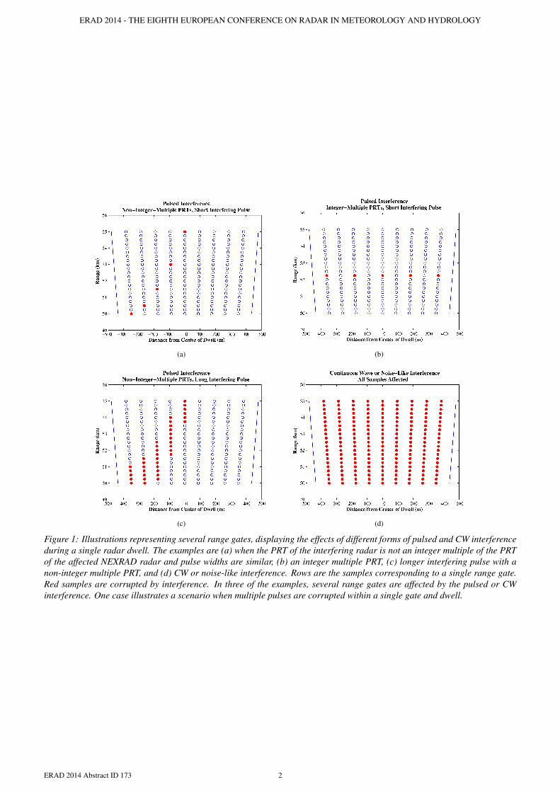
Three types of interference are considered in this study: pulsed, continuous wave (CW), and noise-like. The main focusis pulsed interference, especially from ASR radars and from other NEXRAD radars, but continuous-wave interference canbe seen as an extreme type of pulsed interference when all of the samples at a particular range gate are affected. Noise-likeinterference also affects all of the samples at a particular range gate, but is incoherent and is treated separately. The differenttypes of interference are explored in a set of illustrations presented in Figure 1.

The first example is of pulsed interference from a radar where the pulse repetition time (PRT) of the interfering radar isnot an integer multiple of the PRT of the receiving radar. The pulse width of the interfering radar is also similar in width orshorter than the pulse width of the affected NEXRAD radar (1.57 µs for short pulse or 4.71 µs for long pulse), correspondingto interference from an ASR-8, ASR-9, or another NEXRAD radar. Figure 1(a) shows several range gates from this particularexample. The columns in the figure represent the sampled returns from pulses transmitted by the radar. In the example shown,there are 9 pulses in a dwell. The number of pulses can vary from 3 in the batch mode for Volume Coverage Pattern (VCP) 12to 278 in VCP 32. The radar is rotating as the pulses are transmitted, which causes them to be at slightly different azimuths andconsequently different distances with respect to the center of the dwell. In this case, the center of the dwell is the azimuth of thefifth transmitted pulse and is labeled with a zero on the x-axis of Figure 1(a). The rows correspond to range gates with those atthe top corresponding to range gates that are farther from the radar. Each row contains the samples that are used to estimate themeteorological variables for that particular range gate. The red dots represent samples directly affected by pulsed interference.This type of pulsed interference has the least effect on the estimation of meteorological variables since only one sample at aparticular range gate is affected. We refer to this as single-hit interference because only a single sample at a particular rangegate is corrupted.

The next example is similar to the first one, except the PRT from the interfering radars is an integer multiple of the PRT fromthe NEXRAD radar. When one PRT is an integer multiple of the other PRT, multiple samples can be affected by interference ata single range gate, which is illustrated in Figure 1(b). This leads to larger errors for the meteorological-variable estimates, but

ERAD 2014 Abstract ID 173 1 [email protected]


(a) (b)

(c) (d)

Figure 1: Illustrations representing several range gates, displaying the effects of different forms of pulsed and CW interferenceduring a single radar dwell. The examples are (a) when the PRT of the interfering radar is not an integer multiple of the PRTof the affected NEXRAD radar and pulse widths are similar, (b) an integer multiple PRT, (c) longer interfering pulse with anon-integer multiple PRT, and (d) CW or noise-like interference. Rows are the samples corresponding to a single range gate.Red samples are corrupted by interference. In three of the examples, several range gates are affected by the pulsed or CWinterference. One case illustrates a scenario when multiple pulses are corrupted within a single gate and dwell.

ERAD 2014 Abstract ID 173 2


it affects fewer range gates. This situation should occur significantly less often than the first case since the chance of havingtwo PRTs from independent radars be an exact integer multiple is less common than having non-integer-multiple PRTs.

The next example is also similar to the first one, except that the interfering radar is transmitting a longer pulse. The mostcommon instance of this would be the long pulse utilized on the ASR-11. When the interfering radar transmits a longer pulse,it is more likely that a range gate will have more samples affected because of the larger number of samples that are corruptedby interference. In Figure 1(c), all of the range gates are affected by interference. In this example, range gates farther from theradar are affected with single-hit interference, and the range gates closer to the radar are affected with multiple-hit interference.It is expected that the multiple-hit interference will have a larger effect on the errors of meteorological-variable estimates thanthe single-hit case.

The last case shows the effects of either CW or noise-like interference. Even though these types of interference are different,they both affect all of the samples in every range gate because the interference is constantly being received. Figure 1(d) showsthis case with all of the samples corrupted by interference. Continuous wave interference can be seen as the most extreme typeof multiple-hit pulsed interference.

Through the rest of this study, we focus on the two extremes of single-hit and CW interference. The single-hit case affectsthe errors of meteorological-variable estimates the least with CW interference affecting the them the most, while other typesof multiple-hit interference falling in-between. Noise-like interference is treated separately due to its different characteristics.Although noise-like and CW interference both affect all of the samples in a dwell, the CW interference is at a particularfrequency and shows up as a peak in the Doppler spectrum. Noise-like interference increases the noise power at the receiverand affects all frequencies in the Doppler spectrum equally.

2.2. Applying NEXRAD Technical Requirements to Interference

The purpose of this study is to set interference-to-noise ratio (INR) thresholds based on simulations of meteorologicalvariables (Level II products) using the NEXRAD Technical requirements. There are no particular requirements that specifythe amount of interference allowed, so we derived specific requirements based on the existing ones. The basic precision (orstandard deviation) requirements for each of the six meteorological variables are listed in Table 1. These are the requirements

Table 1: Precision requirements for the six meteorological variables from the WSR-88D System Specification (ROC, 2008).

Base Data Variable Standard DeviationReflectivity For a true spectrum width of 4 m s−1 the standard deviation in the esti-

mate of the reflectivity will be less than or equal to 1 dB at SNR > 10dB (including only the error due to meteorological signal fluctuations).

Mean Radial Velocity For a true spectrum width of 4 m s−1 the standard deviation in the es-timate of the mean radial velocity will be less than or equal to 1.0 ms−1 including quantization errors, for SNR greater than 8 dB.

Spectrum Width For a true spectrum width of 4 m s−1 the standard deviation in the esti-mate of the spectrum width will be less than or equal to 1.0 m s−1 in-cluding quantization errors, for SNR greater than 10 dB.

Differential Reflectivity1 For a spectrum width of 2 m s−1, correlation coefficient ≥ 0.99, anddwell time of 50 ms, the standard deviation in the estimate of the differ-ential reflectivity will be less than 0.3 dB for SNR ≥ 20 dB.

Correlation Coefficient For a true spectrum width of 2 m s−1, correlation coefficient ≥ 0.99,and dwell time of 50 ms, the standard deviation in the estimate of thecorrelation coefficient will be less than 0.006 for SNR ≥ 20 dB.

Differential Phase For a true spectrum width of 2 m s−1, correlation coefficient ≥ 0.99,and dwell time of 50 ms, the standard deviation in the estimate of thedifferential will be less than 2.5◦ for SNR ≥ 20 dB.

that specify the standard deviation of the meteorological-variable estimators under a certain set of conditions. For example,the reflectivity standard deviation requirement is 1 dB at an SNR of 10 dB and a true spectrum width of 4 m s−1. Theother requirements are similar in that the requirement is set for a specific set of conditions, including the true correlationcoefficient for the polarimetric variables. Unfortunately, it is difficult to directly apply these requirements to interference. Weare concerned about the effects of interference at all SNR values, not just the particular ones listed in the requirements. Forexample, the polarimetric-variable requirements are set at an SNR of 20 dB, but interference could cause significant problemsat lower SNR values. Also, for VCP 12, the requirements in Table 1 are barely met; this could lead to a determination whereno interference may be allowed at all. In addition to the standard deviation requirements, there is also a bias requirement forreflectivity estimates that mandates absolute calibration within 1 dB; we are focusing on the precision requirements that apply

1The differential reflectivity requirement is being updated to 0.4 dB by the ROC.



to the estimation (rather than calibration) of the meteorological variables. Our decision is to use the requirements as a startingpoint to find a reasonable way to look at the effects of interference for a wide range of SNR values.

In addition to requirements listed in Table 1, there are also requirements related to ground clutter filtering. In some ways, theeffects of interference are similar to the effects of ground clutter: a non-weather signal is degrading the quality of meteorolog-ical variable estimates. The main difference lies in the fact that there are ground clutter filters in the signal processor that helpto mitigate the effects on the estimates, while there is no such filter for interference signals. The requirements are set assumingthat the user is gaining something from the ground clutter filtering, which results in a relaxation of the normal requirements.Currently, there are no specific filters used to mitigate the effects of electromagnetic interference on NEXRAD radars. Theradial-by-radial noise estimator that is discussed in Section 4 can remove some of the effects of noise-like interference, but theinterference still affects the sensitivity of the radar. Even if there were filters designed specifically to remove interference, theydo not necessarily work the same way as ground clutter filters. For example, a pulsed interference filter could remove verystrong interference spikes but leave weaker (more difficult to detect) spikes that still affect the meteorological variable esti-mates. Another difference is the fact that ground clutter is always present to a certain extent, but siting and spectrum allocationcan be used to mitigate interference. Because of these differences, we adopted the same types of requirements that are used forground clutter filtering, but with somewhat more stringent limits for interference.

The ground clutter requirements are written in terms of “maximum allowable bias in reflectivity estimates due to the cluttersuppression device” (ROC, 2008). We refer to this as the delta bias (∆Bias) since it is in addition to the inherent bias of theestimator. For example, the most stringent clutter requirement for reflectivity is a maximum allowable bias of 1 dB. This meansthat the bias of the estimator with clutter present must be within 1 dB of the inherent bias of the estimator. This requirementstructure also works well for interference since interference is an external source of estimation bias. The key decision thenbecomes setting limits on the ∆Bias for each of the meteorological variables. Historically, the ∆Bias limits for interferencehave been set based on the standard deviation limits from the requirements listed in Table 1. This results in a ∆Bias limit of1 dB for reflectivity, and 1 m s−1 for both velocity and spectrum width at all SNRs. The ∆Bias for reflectivity is measuredin dB rather than dBZ because it is the ratio of two linear values (in logarithmic units). These values were used in NTIAReport TR-06-444 (2006) for reflectivity and spectrum width. We also found the same limits suggested by Dale Sirmans ininternal documents that were written during his long career at the Radar Operations Center. These limits are more stringentthan the ground clutter limits that are stated in the requirements document, but they are directly related to the standard deviationrequirements (listed in Table 1).

In the same way that ∆Bias measures the deviation from the inherent bias of the estimator, we can also look at deviation fromthe inherent standard deviation of the estimator. For ground clutter, this is described in the requirements as “bias and standarddeviation contributions by the clutter suppression device” (ROC, 2008). For interference, we are capturing bias and standarddeviation contributed in addition to the inherent bias and standard deviation of the estimators. The delta standard deviation(∆SD) is similar to the ∆Bias but can be used in particular situations where the ∆Bias is not sensitive to interference. Wewill see examples of this for the radial velocity pulsed interference simulation in Section 3. Just as with the ∆Bias, we need todetermine limits for ∆SD that are reasonable and are derived from the system requirements. Historically, the same limits areused for ∆SD that are used for ∆Bias. This gives a consistent way to quantify the effects of interference on both the bias andstandard deviation of the meteorological-variable estimators.

Limits were given for reflectivity, velocity, and spectrum width, but not for the polarimetric-variable estimators. This isexamined in more detail in Section 3, but the main reason is due to the very large biases and standard deviations of thepolarimetric variables at low SNR values. The inherent biases and standard deviations at low SNR are many times larger thanthe standard deviation requirements stated in Table 1. In contrast, the inherent biases and standard deviations for reflectivity,velocity, and spectrum width at low SNR are only a few times larger than the standard deviation requirements. In general, thepolarimetric-variable estimators are much more sensitive to noise, which makes it very difficult and somewhat meaningless tomeasure changes in ∆Bias or ∆SD at low SNR. We will focus on reflectivity, velocity, and spectrum width when analyzingthe simulations. Because all of these variables are only computed using the horizontal polarization channel, the horizontalinterference power should be the main focus when utilizing the INR thresholds.

The 1-dB and 1-m s−1 limits are reasonable for non-meteorological interference that comes from an external source, butis not necessarily present at all sites like ground clutter. For completeness, we also address two other possible ∆Bias and∆SD limits in the main report (Curtis and Isom, 2014), but omit the results for this discussion. In the report, we include∆Bias limits of 2 dB and 0.5 dB for reflectivity and ∆Bias and ∆SD limits of 2 m s−1 and 0.5 m s−1 for velocity andspectrum width. These additional values provide a way to examine the effects of varying the ∆Bias and ∆SD limits on theINR thresholds.



2.3. Volume Coverage Patterns

Now that we have looked at the different types of interference and the derived requirements that are used to determine theINR thresholds, we can identify the scanning strategies that are most sensitive to interference. By focusing on the most sensi-tive strategies, we can capture the effects of interference without looking at every possible scanning strategy or combination ofacquisition parameters. NEXRAD operational VCPs fall into two major categories: precipitation and clear air. Clear-air VCPsare used when there is little or no precipitation, and sometimes in cases of light snow: VCP 31 and VCP 32. PrecipitationVCPs are used when significant precipitation is present: VCP 11, VCP 12, VCP 21, VCP 121, VCP 211, VCP 212, and VCP221.

The VCPs are collections of sweeps (360◦ revolutions of the antenna) at different (constant) elevation angles (also calledcuts). At low elevation angles, there can be more than one sweep. For example, a split sweep (also referred to as a “split cut”)is made up of two sweeps at the same elevation angle with a different PRT for each sweep. The first sweep, or surveillancesweep, uses a long PRT, while the second sweep, or Doppler sweep, uses a shorter PRT.

Another type of sweep that uses two PRTs is the batch sweep. The batch sweep alternates sets of long and short PRTs duringa single sweep. The two sets of pulses from both PRTs form a single dwell for processing. As with the split sweep, the longPRT pulses are referred to as the “surveillance pulse” and short PRT pulses are the “Doppler pulse”. The last type of sweep,continuous Doppler, is used at high elevation angles and consists of a single PRT.

At each elevation angle in a VCP, the meteorological-variable estimates are censored so the estimates with poor quality dueto noise contamination are eliminated from the display. The VCP has a set of SNR thresholds at each elevation to determinewhich estimates are visible. For example, the default SNR threshold for the surveillance sweep that is part of the 0.5◦ splitsweep from VCP 12 is 2.0 dB. For the Doppler sweep that is also part of the same split sweep, the default SNR threshold is3.5 dB. Although the default values can be changed by the forecasters, we use the default values in the simulations becausethey are seldom modified in practice. These SNR thresholds represent the lower end of SNR values where estimates aredisplayed and are where the effects of interference are most pronounced.

For this study, we identified one clear-air and one precipitation VCP that are especially susceptible to interference. Clear-airVCP 31 has the lowest default SNR threshold at 0 dB. This is the same VCP that was used in the meteorological radar testingsection of ITU-R M.1464 (1998). The low default SNR threshold makes it more sensitive to interference than the other clear-air VCP (VCP 32). We chose precipitation VCP 12 because it has the fastest update rate (fewer pulses per dwell), is used themost often for the convective events associated with severe weather, and the standard deviations of the estimators barely meetrequirements. Both of the VCPs are described in Tables 2 and 3, respectively, and particular elevation sweeps are chosen forlater exploration through simulations. The split sweep surveillance and Doppler scans are abbreviated with SS and SD, and

Table 2: Scan parameters for VCP 31 for the surveillance and Doppler sweeps at the lowest elevation angles.

Scan Type Elevation PRT (ms) va m s−1 Pulses SNRth (dB) OutputSS 0.5-2.5◦ 3.12 8.43 63 0.0 Z,ZDR,ΦDP,ρhvSD 0.5-2.5◦ 2.25 11.7 87 0.0 v,σv

Table 3: Scan parameters for VCP 12 for the lowest elevation split sweep (0.5◦) and the lowest elevation batch sweep (1.8◦).

Scan Type Elevation PRT (ms) va m s−1 Pulses SNRth (dB) OutputSS 0.5◦ 3.12 8.44 15 2.0 Z,ZDR,ΦDP,ρhvSD 0.5◦ 0.986 26.7 40 3.5 v,σvBS 1.8◦ 3.12 8.44 3 3.5 Z,ZDR,ΦDP,ρhvBD 1.8◦ 0.986 26.7 29 3.5 Z,v,σv ,ZDR,ΦDP,ρhv

the batch sweep scans are similarly represented by BS and BD. Higher elevation scans are not considered in this study.

An additional attribute of VCP 31 that needs to be considered is that it utilizes a 4.71-µs transmitted pulse (long pulse)instead of the 1.57-µs transmitted pulse (short pulse) used for the other VCPs. This leads to a lower noise power whencompared to the VCPs that use the short pulse after the matched filter is applied. The simulations that were implemented tostudy the effects of interference set the SNR based on the post-matched-filter noise power. This should be taken into accountwhen employing the INR thresholds because the same level of interference will result in a different INR threshold (INRth)for different pulse lengths. The noise power depends on the matched-filter bandwidth, which is typically tied to the length ofthe pulse (long or short).

The rest of the paper is organized as follows. Section 3 describes the methods used to simulate time series data and howthe INR thresholds are derived from the simulations. Section 4 discusses the effects of noise-like interference on the system.Section 5 explores some possible future changes to the NEXRAD system that could influence the results. Finally, Section 6summarizes the effects of interference and our approach to quantifying them.



3. Pulsed and Continuous Wave Interference

In this section, the effects of pulsed and CW interference are studied using time series simulations. First, the time seriessimulations are described including models for both types of interference. The polarimetric variables are then discussedfocusing on why they are not used to determine INR thresholds. The next two sections summarize the results for pulsed andCW interference, respectively, and provide the INR thresholds that are based on the simulations.

3.1. Simulation Methodology and Theory

The weather simulator developed for this study utilizes a technique developed by Zrnic (1975), but expanded to includepolarimetric signals (Galati and Pavan, 1995). The weather simulator produces dual-polarization time series data based onthe true values of all six meteorological variables (Z, v, σv , ZDR, ΦDP, ρhv), and interference models are used to generatecorrupting signals, which are then added to the simulated weather. The algorithms used to process the data in the simulationsare the same algorithms implemented on the NEXRAD radars. Because the interference signals are relatively simple to model,simulations can accurately capture the effects of interference over a wide range of conditions. A block diagram of the weather-interference simulator is presented in Figure 2, which will be referenced in the subsequent discussion.

Figure 2: A block diagram of the weather-interference simulator. Two paths for the simulated weather data are maintained toallow for comparisons and direct calculations of the statistical impact to the meteorological variables.

Block 1, the Weather Simulation, takes the true values of the meteorological variables (Z, v, σv , ZDR, ΦDP, ρhv) as inputas well as the number of samples (M ), the noise power (N ), and signal-to-noise ratio (SNR). For the simulations and withoutloss of generality, the horizontal and vertical channel noise powers are assumed to be the same. Two complex time serieschannels are produced at the output representing the horizontal and vertical channel data. For this study, 100,000 realizationsare simulated to achieve accurate statistical results.

Block 2 generates the interference data for both pulsed and continuous wave interference. The noise-like interference caseis not considered in the simulations and is addressed separately in Section 4. Pulsed interference is modeled as a single hitwith random phase φp. The interference powers, Ih and Iv, are used in the definitions of the INR (INR = Ih/N ) and thedifferential interference ratio (IDR = Ih/Iv). Note that the INR value is taken as the direct ratio between the interference andnoise powers, and is based on the horizontal channel. That is, INR is equal to one (or zero dB) when the interference fromthe horizontal channel is equal to the noise. IDR is defined as the ratio between the horizontal and vertical channel interferencepowers; thus, the vertical interference power is determined by the horizontal interference power and the IDR.

To accurately represent single-hit pulsed interference, the temporal location of the interference pulse within the dwell isselected at random and all other samples in the dwell are set to zero. The pulsed-interference time series signals at a particularrange gate are defined in Equation 3.1:

Vh(m) =

{ √Ihexp [jφp] , if m = k

0, otherwise,

Vv(m) =

{ √Ivexp [j(φp + α)] , if m = k

0, otherwise

(3.1)

where m is the sample index from 1 to M , j =√−1, φp is a uniform random variable between 0 and 2n, and k is an integer-

valued random variable between 1 and M . The additional α in the vertical channel captures the phase difference between thechannels based on the transmitted polarization.

CW interference is modeled as a single tone (frequency) that is within the passband of the radar receiving the interference.The interfering signal appears at an apparent Doppler velocity vCW. The initial phase of the tone, φCW, is a uniform randomvariable between 0 and 2n, and the interference powers, Ih and Iv, are again defined by the INR and IDR values.



A mathematical expression for the CW-interference time series signals is given in Equation 3.2:

Vh(m) =√Ihexp [−j(4πvCWmTs/λ+ φCW] ,

Vv(m) =√Ivexp [−j(4πvCWmTs/λ+ φCW + α]

(3.2)

where Ts is the PRT, m is the sample index from 1 to M , and λ is the transmitter/radar wavelength. The α value captures theeffect of the transmitted polarization of the interference. In both the pulsed and CW interference cases, horizontal and verticalcomplex time series data are produced.

One branch of the simulator shown in Figure 2 preserves the weather time series, while the other sums the interferencesignal with the weather. Preserving both the original and corrupted signals allows for direct statistical comparisons to bemade. The subsequent stage of the simulator (Block 3) calculates the traditional weather radar variables (Z, v, σv , ZDR,ΦDP, ρhv) for the corrupted and uncorrupted signal paths using processing based on the Radar Data Acquisition (RDA) unitof the NEXRAD receiver subsystem. In Block 4, the bias and standard deviation are computed for each of the meteorologicalvariables. Block 4(b) computes the inherent bias and standard deviation of the estimators, and Block 4(a) includes the additionalbias and standard deviation introduced by the interference. Then, in Block 5, the ∆Bias and ∆SD are calculated for eachmeteorological variable, which is denoted by the ∆θ symbol in the diagram. The difference calculation allows for the extentof the impact of the interference on the meteorological variables to be ascertained while accounting for the inherent bias andstandard deviation of the estimators themselves. Statistics are then examined and collated to create meaningful illustrationsand to find INRth values.

3.2. Polarimetric Variables

As mentioned in the previous section, the polarimetric variables are not used to determine the INR thresholds. In thissection, we show an example using the differential reflectivity (ZDR) to better illustrate some of the issues with utilizing thepolarimetric variables for this purpose. The other two polarimetric variables, differential phase and correlation coefficient,behave very similarly to ZDR at low SNR values and do not add significantly to the discussion.

Figure 3 shows the bias and standard deviation of ZDR over a wide range of INR values when pulsed interference is addedto the weather signal. Shown in the figure is the total bias and standard deviation from both signals, and not the ∆Bias and∆SD that will be used in subsequent sections. Figure 3(a) and Figure 3(c) show the bias and standard deviation with atrue ZDR of 0.2 dB and an IDR of 0 dB, while Figure 3(b) and Figure 3(d) utilize the same statistical parameters, except thetrue ZDR is 4.5 dB. The SNR for the weather signal is kept constant at 3.5 dB based on the SNR threshold for the Dopplerpart for the batch sweep (BD) in VCP 12. The true ZDR of 0.2 dB would most often occur in light rain, and the true ZDR of4.5 dB is a more extreme case that could occur in certain types of hail.

There are two main issues with using the polarimetric variables for determining INR thresholds. The first is the variabilityin the bias and standard deviation at low SNR values. This variability is apparent in all four plots in Figure 3. This variabilitywould lead to extremely low INR thresholds that were not due to interference, but instead to spikes in the bias and standarddeviation values. One solution to the variability issue would be to significantly increase the number of realizations in thesimulations to attempt to only capture the effects of interference. Running enough simulations is probably not practical inthis case because of the other issue with using the polarimetric variables: the standard deviations from the requirements arevery small compared to the biases and standard deviations shown in Figure 3, making the measurement meaningless. Forexample, the standard deviation of the weather signal alone in Figure 3(c) is around 6 dB (and even larger for Figure 3(d)).The standard deviation requirement of 0.3 dB is also shown in these two plots. The standard deviation at low SNR values isso large compared to the ∆SD limit of 0.3 dB that it makes the ∆SD irrelevant.

The difference between the polarimetric variables and the meteorological variables (Z, v, σv) is this large discrepancybetween the standard deviation requirements and the bias and standard deviations at low SNR. The requirements for thepolarimetric variables are set at a higher SNR value (20 dB) than the 8 or 10 dB for the other variables. Additionally, thepolarimetric variables are just more sensitive to noise which makes it extremely difficult to measure the effects of interferenceat low SNR values. For these reasons, the INR thresholds are determined based on reflectivity, velocity and spectrum width.

3.3. Pulsed Interference

Pulsed interference occurs when a surveillance radar interferes with another surveillance radar. This study specificallyfocuses on the interference from ASR-8, 9, and 11 radars on NEXRAD radars, as well as the interference from NEXRADradars on other NEXRAD radars. As described in the simulation methodology, pulsed interference is modeled as a single hitat one range gate. This is the smallest effect that pulsed interference can have on a range gate, but this is a reasonable placeto start since pulsed interference only affects a relatively small fraction of range gates in a sweep. This section examines theeffects of pulsed interference on reflectivity, velocity, and spectrum width, and provides INR thresholds based on derivedrequirements. The results will be summarized to show the minimum INR thresholds for the three scan types: VCP 12 batch



(a) (b)

(c) (d)

Figure 3: The ZDR bias and standard deviation as a function of INR with a true ZDR of 0.2 dB, (a) and (c), and 4.5 dB, (b)and (d). The solid red horizontal line represents the mean inherent bias or standard deviation without interference, and thedashed horizontal line represents the 0.3 dB threshold based on the dual-polarization requirements in Table 1.



sweep, VCP 12 split sweep, and VCP 31 split sweep. Finally, the fraction of range gates corrupted by pulsed interference fordifferent interfering radars is addressed.

3.3.1. Reflectivity

Reflectivity is one of the most utilized and intuitive meteorological variables. It measures the backscattering cross section ofthe hydrometeors in a resolution volume and is derived from the received signal power. Reflectivity is used in many downstreamalgorithms such as rainfall estimation, which aid in the delivery of flood watches and warnings. In this section, we examinethe effects of pulsed interference on reflectivity estimates by looking at ∆Bias and ∆SD.

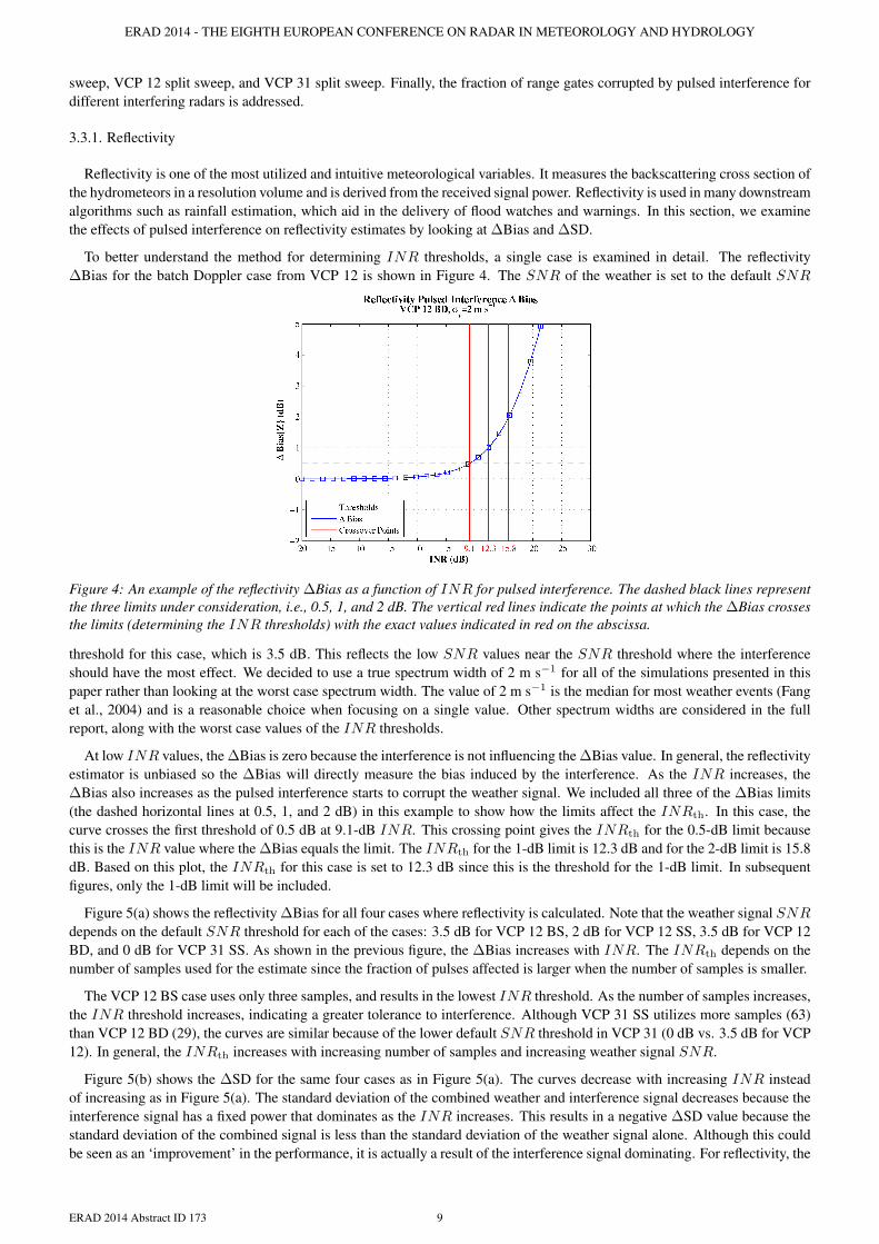
To better understand the method for determining INR thresholds, a single case is examined in detail. The reflectivity∆Bias for the batch Doppler case from VCP 12 is shown in Figure 4. The SNR of the weather is set to the default SNR

Figure 4: An example of the reflectivity ∆Bias as a function of INR for pulsed interference. The dashed black lines representthe three limits under consideration, i.e., 0.5, 1, and 2 dB. The vertical red lines indicate the points at which the ∆Bias crossesthe limits (determining the INR thresholds) with the exact values indicated in red on the abscissa.

threshold for this case, which is 3.5 dB. This reflects the low SNR values near the SNR threshold where the interferenceshould have the most effect. We decided to use a true spectrum width of 2 m s−1 for all of the simulations presented in thispaper rather than looking at the worst case spectrum width. The value of 2 m s−1 is the median for most weather events (Fanget al., 2004) and is a reasonable choice when focusing on a single value. Other spectrum widths are considered in the fullreport, along with the worst case values of the INR thresholds.

At low INR values, the ∆Bias is zero because the interference is not influencing the ∆Bias value. In general, the reflectivityestimator is unbiased so the ∆Bias will directly measure the bias induced by the interference. As the INR increases, the∆Bias also increases as the pulsed interference starts to corrupt the weather signal. We included all three of the ∆Bias limits(the dashed horizontal lines at 0.5, 1, and 2 dB) in this example to show how the limits affect the INRth. In this case, thecurve crosses the first threshold of 0.5 dB at 9.1-dB INR. This crossing point gives the INRth for the 0.5-dB limit becausethis is the INR value where the ∆Bias equals the limit. The INRth for the 1-dB limit is 12.3 dB and for the 2-dB limit is 15.8dB. Based on this plot, the INRth for this case is set to 12.3 dB since this is the threshold for the 1-dB limit. In subsequentfigures, only the 1-dB limit will be included.

Figure 5(a) shows the reflectivity ∆Bias for all four cases where reflectivity is calculated. Note that the weather signal SNRdepends on the default SNR threshold for each of the cases: 3.5 dB for VCP 12 BS, 2 dB for VCP 12 SS, 3.5 dB for VCP 12BD, and 0 dB for VCP 31 SS. As shown in the previous figure, the ∆Bias increases with INR. The INRth depends on thenumber of samples used for the estimate since the fraction of pulses affected is larger when the number of samples is smaller.

The VCP 12 BS case uses only three samples, and results in the lowest INR threshold. As the number of samples increases,the INR threshold increases, indicating a greater tolerance to interference. Although VCP 31 SS utilizes more samples (63)than VCP 12 BD (29), the curves are similar because of the lower default SNR threshold in VCP 31 (0 dB vs. 3.5 dB for VCP12). In general, the INRth increases with increasing number of samples and increasing weather signal SNR.

Figure 5(b) shows the ∆SD for the same four cases as in Figure 5(a). The curves decrease with increasing INR insteadof increasing as in Figure 5(a). The standard deviation of the combined weather and interference signal decreases because theinterference signal has a fixed power that dominates as the INR increases. This results in a negative ∆SD value because thestandard deviation of the combined signal is less than the standard deviation of the weather signal alone. Although this couldbe seen as an ‘improvement’ in the performance, it is actually a result of the interference signal dominating. For reflectivity, the



(a) (b)

Figure 5: Reflectivity (a)∆Bias and (b)∆SD as a function of INR for pulsed interference depicting four cases associated withVCP 12 and 31. The 1-dB limit is denoted by the dashed horizontal line. An increase in tolerance is visible as the samplesize increases for the ∆Bias plot, while the ∆SD curves never cross the limit, and thus no INRth is assigned in any of the∆SD cases.

∆Bias will be used to set the INR thresholds, and no INR thresholds for ∆SD will be assigned for any of the cases becausethe threshold is not crossed.

The INR thresholds for reflectivity ∆Bias are presented in Table 4 at the end of this section, along with results for radialvelocity and spectrum width. These are the thresholds for a spectrum width of 2 m s−1, and ∆Bias and ∆SD limits of 1 dB.The 1-dB limit for ∆SD was not exceeded for any of the test cases and is omitted from the table. The table is organized in ahierarchical manner with VCP as the primary designator, followed by scan type. Dark gray cells indicate that the scan is notused to calculate reflectivity; all four cases where reflectivity is calculated are shown in the tables. The lowest INRth appearsin the VCP 12 BS case with a value of 3.9 dB.

3.3.2. Radial Velocity

The radial velocity estimator measures the mean velocity of the hydrometeors within the resolution volume, in the directionof the radar radial. Detection of wind shear and mesocyclone vortices are important uses of the radial velocity estimator, andbiases in the measurement of velocity can impact the ability to identify areas of potential risk for life and property. Radialvelocity is not a biased estimator, meaning that any bias observed during the interference study is due to the influence of thecorrupting signal. As with reflectivity, the effects of pulsed interference on ∆Bias and∆SD are examined.

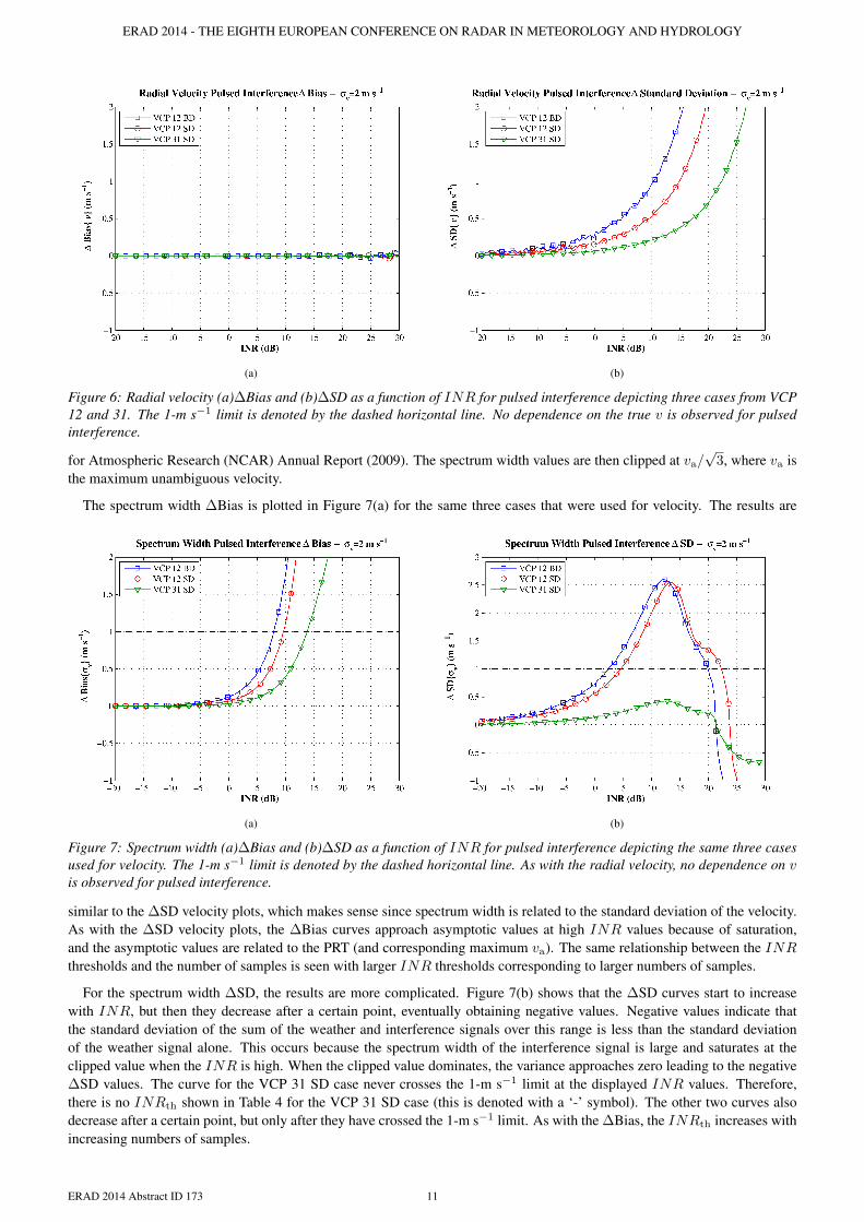
The radial velocity ∆Bias is not especially illuminating because pulsed interference does not induce a bias in the velocityestimator. Figure 6(a) shows the ∆Bias for the three cases where velocity is estimated. As with the reflectivity simulations,the weather signal SNR is set based on the default SNR thresholds: 3.5 dB for VCP 12 BD and VCP 12 SD, and 0 dB forVCP 31 SD. Because pulsed interference is an impulse in the time domain, it appears flat in the spectral domain. This meansthat the effects of increasing INR are similar to the effects of increased noise. The bias is zero, but the standard deviationof the estimator increases. Figure 6(b) illustrates the effects of pulsed interference on the velocity ∆SD. As expected, the∆SD increases with increasing INR. Although it is not shown in the figure, the ∆SD curves approach asymptotic values atvery large INRs because the standard deviation saturates when the spectrum becomes completely flat. The asymptotic valuesdepend on the PRT since the maximum unambiguous velocity determines the width of the spectrum. We will also see the effectsof this flat spectrum when we examine the spectrum width estimator. As with the reflectivity, the ∆SD INRth increases withincreasing number of samples. The VCP 12 BD case (29 samples) has the lowest INRth, and the VCP 31 SD case (87samples) has the largest INRth.

The values of the INR thresholds determined from the ∆SD curves are captured in Table 4. No ∆Bias values are presentedin the table. The INR thresholds are higher for velocity than for reflectivity, which indicates that the reflectivity estimator ismore sensitive to pulsed interference.

3.3.3. Spectrum Width

Spectrum width provides valuable information about turbulence and velocity dispersion within the resolution volume. Inorder to match the processing on the NEXRAD radars, the same hybrid spectrum width estimator was utilized in the simulationsthat is currently implemented on the NEXRAD system. This estimator returns either the R1/R3, R1/R2, or R0/R1 estimatedepending on a preliminary spectrum width calculation. The algorithm was implemented as described in the National Center



(a) (b)

Figure 6: Radial velocity (a)∆Bias and (b)∆SD as a function of INR for pulsed interference depicting three cases from VCP12 and 31. The 1-m s−1 limit is denoted by the dashed horizontal line. No dependence on the true v is observed for pulsedinterference.

for Atmospheric Research (NCAR) Annual Report (2009). The spectrum width values are then clipped at va/√

3, where va isthe maximum unambiguous velocity.

The spectrum width ∆Bias is plotted in Figure 7(a) for the same three cases that were used for velocity. The results are

(a) (b)

Figure 7: Spectrum width (a)∆Bias and (b)∆SD as a function of INR for pulsed interference depicting the same three casesused for velocity. The 1-m s−1 limit is denoted by the dashed horizontal line. As with the radial velocity, no dependence on vis observed for pulsed interference.

similar to the ∆SD velocity plots, which makes sense since spectrum width is related to the standard deviation of the velocity.As with the ∆SD velocity plots, the ∆Bias curves approach asymptotic values at high INR values because of saturation,and the asymptotic values are related to the PRT (and corresponding maximum va). The same relationship between the INRthresholds and the number of samples is seen with larger INR thresholds corresponding to larger numbers of samples.

For the spectrum width ∆SD, the results are more complicated. Figure 7(b) shows that the ∆SD curves start to increasewith INR, but then they decrease after a certain point, eventually obtaining negative values. Negative values indicate thatthe standard deviation of the sum of the weather and interference signals over this range is less than the standard deviationof the weather signal alone. This occurs because the spectrum width of the interference signal is large and saturates at theclipped value when the INR is high. When the clipped value dominates, the variance approaches zero leading to the negative∆SD values. The curve for the VCP 31 SD case never crosses the 1-m s−1 limit at the displayed INR values. Therefore,there is no INRth shown in Table 4 for the VCP 31 SD case (this is denoted with a ‘-’ symbol). The other two curves alsodecrease after a certain point, but only after they have crossed the 1-m s−1 limit. As with the ∆Bias, the INRth increases withincreasing numbers of samples.



The ∆SD provides the minimum spectrum width INR thresholds in the cases where it is defined, and the ∆Bias providesthe minimum threshold in the VCP 31 SD case. The spectrum width estimator is the most sensitive to interference for the twoVCP 12 cases, but reflectivity is the driver for VCP 31 case. The sensitivity of the spectrum width estimator to interference isconsistent with the findings in ITU-R M.1464 (1998). The INR thresholds are captured in Table 4 at the end of this section,which combines the results for all three meteorological variables.

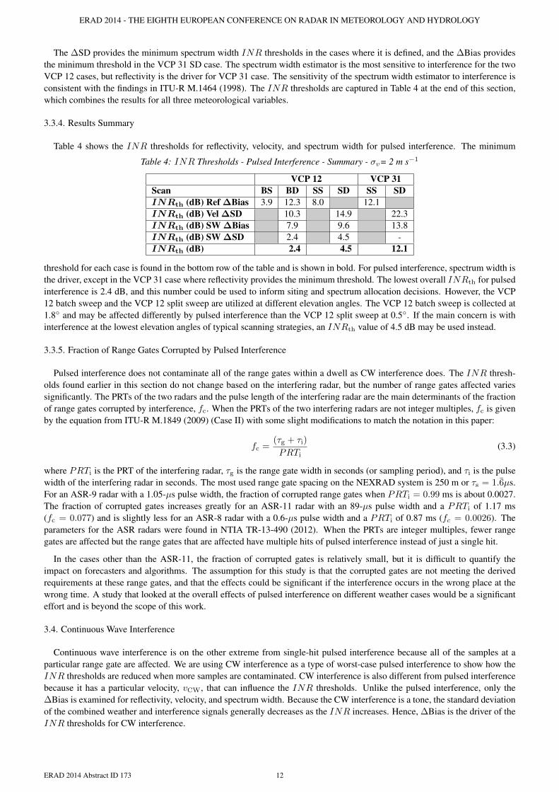
3.3.4. Results Summary

Table 4 shows the INR thresholds for reflectivity, velocity, and spectrum width for pulsed interference. The minimum

Table 4: INR Thresholds - Pulsed Interference - Summary - σv= 2 m s−1

VCP 12 VCP 31Scan BS BD SS SD SS SDINRth (dB) Ref ∆Bias 3.9 12.3 8.0 12.1INRth (dB) Vel ∆SD 10.3 14.9 22.3INRth (dB) SW ∆Bias 7.9 9.6 13.8INRth (dB) SW ∆SD 2.4 4.5 -INRth (dB) 2.4 4.5 12.1

threshold for each case is found in the bottom row of the table and is shown in bold. For pulsed interference, spectrum width isthe driver, except in the VCP 31 case where reflectivity provides the minimum threshold. The lowest overall INRth for pulsedinterference is 2.4 dB, and this number could be used to inform siting and spectrum allocation decisions. However, the VCP12 batch sweep and the VCP 12 split sweep are utilized at different elevation angles. The VCP 12 batch sweep is collected at1.8◦ and may be affected differently by pulsed interference than the VCP 12 split sweep at 0.5◦. If the main concern is withinterference at the lowest elevation angles of typical scanning strategies, an INRth value of 4.5 dB may be used instead.

3.3.5. Fraction of Range Gates Corrupted by Pulsed Interference

Pulsed interference does not contaminate all of the range gates within a dwell as CW interference does. The INR thresh-olds found earlier in this section do not change based on the interfering radar, but the number of range gates affected variessignificantly. The PRTs of the two radars and the pulse length of the interfering radar are the main determinants of the fractionof range gates corrupted by interference, fc. When the PRTs of the two interfering radars are not integer multiples, fc is givenby the equation from ITU-R M.1849 (2009) (Case II) with some slight modifications to match the notation in this paper:

fc =(τg + τi)

PRTi(3.3)

where PRTi is the PRT of the interfering radar, τg is the range gate width in seconds (or sampling period), and τi is the pulsewidth of the interfering radar in seconds. The most used range gate spacing on the NEXRAD system is 250 m or τs = 1.6µs.For an ASR-9 radar with a 1.05-µs pulse width, the fraction of corrupted range gates when PRTi = 0.99 ms is about 0.0027.The fraction of corrupted gates increases greatly for an ASR-11 radar with an 89-µs pulse width and a PRTi of 1.17 ms(fc = 0.077) and is slightly less for an ASR-8 radar with a 0.6-µs pulse width and a PRTi of 0.87 ms (fc = 0.0026). Theparameters for the ASR radars were found in NTIA TR-13-490 (2012). When the PRTs are integer multiples, fewer rangegates are affected but the range gates that are affected have multiple hits of pulsed interference instead of just a single hit.

In the cases other than the ASR-11, the fraction of corrupted gates is relatively small, but it is difficult to quantify theimpact on forecasters and algorithms. The assumption for this study is that the corrupted gates are not meeting the derivedrequirements at these range gates, and that the effects could be significant if the interference occurs in the wrong place at thewrong time. A study that looked at the overall effects of pulsed interference on different weather cases would be a significanteffort and is beyond the scope of this work.

3.4. Continuous Wave Interference

Continuous wave interference is on the other extreme from single-hit pulsed interference because all of the samples at aparticular range gate are affected. We are using CW interference as a type of worst-case pulsed interference to show how theINR thresholds are reduced when more samples are contaminated. CW interference is also different from pulsed interferencebecause it has a particular velocity, vCW, that can influence the INR thresholds. Unlike the pulsed interference, only the∆Bias is examined for reflectivity, velocity, and spectrum width. Because the CW interference is a tone, the standard deviationof the combined weather and interference signals generally decreases as the INR increases. Hence, ∆Bias is the driver of theINR thresholds for CW interference.



3.4.1. Reflectivity

The reflectivity ∆Bias is displayed in Figure 8 for the same four cases that were utilized in the pulsed interference simula-tions. The curves indicate the same dependence of ∆Bias on INR that we saw for pulsed interference. The main difference

Figure 8: Reflectivity ∆Bias as a function of INR for CW interference depicting the four cases from VCP 12 and 31. The1-dB limit is denoted by the dashed horizontal line. Note the lower tolerance for CW interference as compared to the pulsedinterference in Figure 5(a).

is that the INR thresholds are lower for CW interference than for pulsed interference. Another difference is that the defaultSNR thresholds have more effect on the INR thresholds than the number of samples. Notice that the lowest INRth occursfor the VCP 31 SS case with a default SNR threshold of 0 dB. The next highest INRth is the VCP 12 SS case with a de-fault SNR threshold of 2 dB. The highest INR thresholds correspond to the two cases with a default SNR threshold of 3.5dB, VCP 12 BD and VCP 12 BS. Between these two, the highest INRth corresponds to the case with the fewest number ofsamples, VCP 12 BS. For the reflectivity estimator, the interference velocity, vCW, does not affect the results.

The INR thresholds for all four cases are shown in Table 5, along with results for the radial velocity and spectrum widthestimators. These results are for a true spectrum width of 2 m s−1; additional results for other spectrum widths and the 0.5 and2-dB limits are presented in the full report.

3.4.2. Radial Velocity

The velocity ∆Bias for the VCP 12 BD case is shown in Figure 9(a). This is different from the pulsed interference figure

(a) (b)

Figure 9: Radial velocity (a)∆Bias as a function of INR for the VCP 12 batch Doppler case depicting various values of ∆vand (b)INR thresholds as a function of ∆v. The upward trend at high ∆v values is a result of the relationship between theoverlaid echoes at those particular signal-to-interference ratios in (b). The 1-m s−1 limit is presented as the dashed black linein (a).



because only one case (VCP 12 BD) is shown with four different ∆v values. ∆v is the absolute value of the difference betweenthe interference velocity and the weather velocity. The ∆Bias curves approach an asymptote equal to the ∆v values at highINR. As mentioned previously, the interference velocity, vCW, does have an effect on the INR thresholds, and this is reflectedin the different INR thresholds for different ∆v values. Because of this dependence, the effect on the INR thresholds will befurther explored for a complete range of velocities.

Figure 9(b) illustrates the dependence of the INRth on ∆v from 0 m s−1 to va. One would anticipate that the 1-m s−1 limitwould be met at increasingly lower INR values as the ∆v term increases. However, larger ∆v values do not result in theminimum INR value. Instead, an upward trend can be observed at large ∆v values. This upward trend is due to the relationshipbetween the strength of the weather and interference signals as well as the ∆v parameter, and can be explored through the useof a phasor diagram. Because there are multiple interference thresholds for the same case, we need to determine a method tochoose the overall INRth. By picking the worst case value from Figure 9(b), we can ensure that the velocity meets the derivedrequirements for all possible values of ∆v (unknown in practice). In this case, the INR thresholds are relatively flat aroundva/2, so it seems reasonable to choose the worst case value.

Table 5 contains the worst case INRth values for all three velocity cases. The values are very similar for all three cases andare lower than the reflectivity INR thresholds. This shows that the velocity estimator is more sensitive to CW interferencethan the reflectivity estimator.

3.4.3. Spectrum Width

The spectrum width ∆Bias displayed in Figure 10(a) also shows a dependence on ∆v similar to the velocity. The figuredisplays only one case (VCP 12 BD) for four ∆v values. The dependence is more complicated because it increases with INR,

(a) (b)

Figure 10: Spectrum width (a)∆Bias as a function of INR for the VCP 12 batch Doppler case depicting various values of∆v and (b)INR thresholds as a function of ∆v. As with the radial velocity ∆Bias curves, a dependence on the ∆v term isevident. The 1-m s−1 limit is depicted for both positive and negative values with the two dashed black lines in (a).

and then converges to a negative value at very high INR. Some of the curves have a peak because of the bimodal nature ofthe combined weather and interference spectrum. When the powers of the two signals are similar and the signals are separatedin the spectrum, the spectrum width values can be large because the velocities are spread out between both signals. As theCW interference starts to dominate, the measured spectrum width approaches zero, which leads to the negative ∆Bias at highINR. Note that the ∆v = va curve crosses the other curves on both sides of the peak. This occurs because of increased use ofthe R1/R2 estimator and results in less sensitivity to interference at larger ∆v. In addition, only three of the curves cross thepositive 1-m s−1 limit, which results in some interesting behavior in Figure 10(b).

Figure 10(b) shows the dependence of the INRth on ∆v for the VCP 12 BD case. The sharp discontinuity in this figure isdue to the fact that the ∆Bias curves do not cross the positive 1-m s−1 limit at small ∆v values, but do eventually cross thenegative 1-m s−1 limit. At the ∆v value where the ∆Bias starts to cross the positive 1-m s−1limit, the INRth abruptly shiftsresulting in the discontinuity. The INRth increases slightly at larger ∆v values. This is similar to the behavior of the velocity∆Bias except that the mechanism is different. As with the velocity, we use the worst case value for the INRth. This ensuresthat the spectrum width meets the derived requirements under all conditions.

Table 5 captures the INR thresholds for spectrum width for all three cases. The spectrum width is the most sensitive to CWinterference, and this is mainly due to the bimodal nature of the combined weather and interference signals.



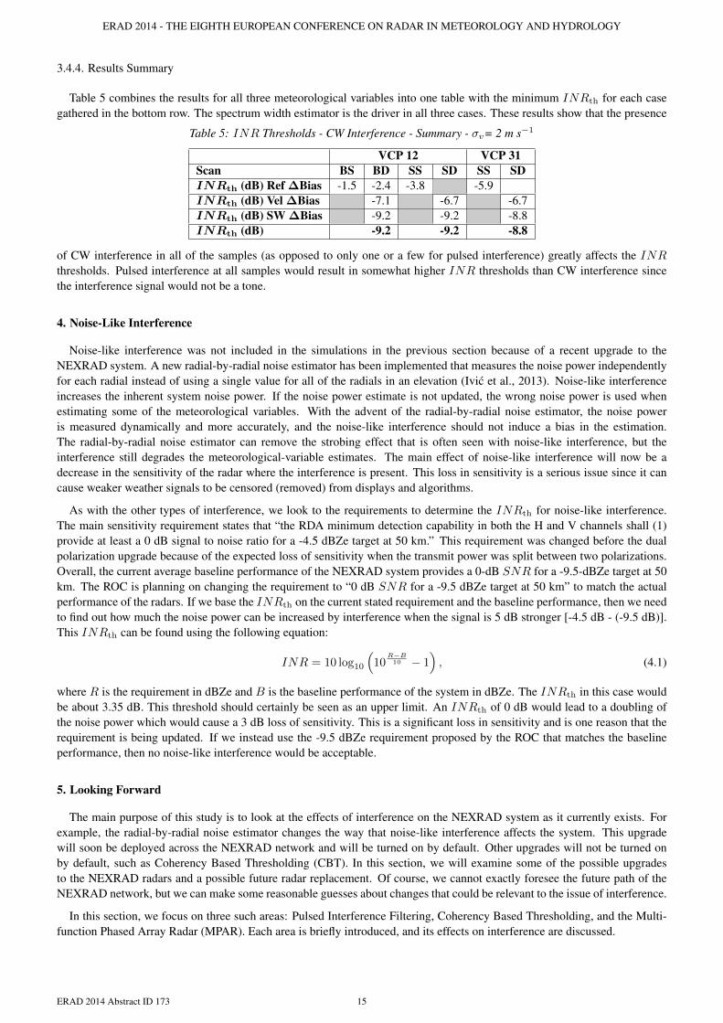
3.4.4. Results Summary

Table 5 combines the results for all three meteorological variables into one table with the minimum INRth for each casegathered in the bottom row. The spectrum width estimator is the driver in all three cases. These results show that the presence

Table 5: INR Thresholds - CW Interference - Summary - σv= 2 m s−1

VCP 12 VCP 31Scan BS BD SS SD SS SDINRth (dB) Ref ∆Bias -1.5 -2.4 -3.8 -5.9INRth (dB) Vel ∆Bias -7.1 -6.7 -6.7INRth (dB) SW ∆Bias -9.2 -9.2 -8.8INRth (dB) -9.2 -9.2 -8.8

of CW interference in all of the samples (as opposed to only one or a few for pulsed interference) greatly affects the INRthresholds. Pulsed interference at all samples would result in somewhat higher INR thresholds than CW interference sincethe interference signal would not be a tone.

4. Noise-Like Interference

Noise-like interference was not included in the simulations in the previous section because of a recent upgrade to theNEXRAD system. A new radial-by-radial noise estimator has been implemented that measures the noise power independentlyfor each radial instead of using a single value for all of the radials in an elevation (Ivic et al., 2013). Noise-like interferenceincreases the inherent system noise power. If the noise power estimate is not updated, the wrong noise power is used whenestimating some of the meteorological variables. With the advent of the radial-by-radial noise estimator, the noise poweris measured dynamically and more accurately, and the noise-like interference should not induce a bias in the estimation.The radial-by-radial noise estimator can remove the strobing effect that is often seen with noise-like interference, but theinterference still degrades the meteorological-variable estimates. The main effect of noise-like interference will now be adecrease in the sensitivity of the radar where the interference is present. This loss in sensitivity is a serious issue since it cancause weaker weather signals to be censored (removed) from displays and algorithms.

As with the other types of interference, we look to the requirements to determine the INRth for noise-like interference.The main sensitivity requirement states that “the RDA minimum detection capability in both the H and V channels shall (1)provide at least a 0 dB signal to noise ratio for a -4.5 dBZe target at 50 km.” This requirement was changed before the dualpolarization upgrade because of the expected loss of sensitivity when the transmit power was split between two polarizations.Overall, the current average baseline performance of the NEXRAD system provides a 0-dB SNR for a -9.5-dBZe target at 50km. The ROC is planning on changing the requirement to “0 dB SNR for a -9.5 dBZe target at 50 km” to match the actualperformance of the radars. If we base the INRth on the current stated requirement and the baseline performance, then we needto find out how much the noise power can be increased by interference when the signal is 5 dB stronger [-4.5 dB - (-9.5 dB)].This INRth can be found using the following equation:

INR = 10 log10

(10

R−B10 − 1

), (4.1)

where R is the requirement in dBZe and B is the baseline performance of the system in dBZe. The INRth in this case wouldbe about 3.35 dB. This threshold should certainly be seen as an upper limit. An INRth of 0 dB would lead to a doubling ofthe noise power which would cause a 3 dB loss of sensitivity. This is a significant loss in sensitivity and is one reason that therequirement is being updated. If we instead use the -9.5 dBZe requirement proposed by the ROC that matches the baselineperformance, then no noise-like interference would be acceptable.

5. Looking Forward

The main purpose of this study is to look at the effects of interference on the NEXRAD system as it currently exists. Forexample, the radial-by-radial noise estimator changes the way that noise-like interference affects the system. This upgradewill soon be deployed across the NEXRAD network and will be turned on by default. Other upgrades will not be turned onby default, such as Coherency Based Thresholding (CBT). In this section, we will examine some of the possible upgradesto the NEXRAD radars and a possible future radar replacement. Of course, we cannot exactly foresee the future path of theNEXRAD network, but we can make some reasonable guesses about changes that could be relevant to the issue of interference.

In this section, we focus on three such areas: Pulsed Interference Filtering, Coherency Based Thresholding, and the Multi-function Phased Array Radar (MPAR). Each area is briefly introduced, and its effects on interference are discussed.



5.1. Pulsed Interference Filtering

There are certainly additional signal processing upgrades that could be made to the system to mitigate the effects of electro-magnetic interference. One area that could be addressed with relatively simple filters is pulsed interference. Strong spikes inthe Level-I (or time series) data can be detected relatively easily, but there are two main issues that can limit the effectivenessof pulsed interference filters. The first issue is determining what to replace the interference spike with if one is detected. Thereare concerns with interpolating across samples at a particular range gate if there are multiple signals present such as weatherand clutter. Interpolating in range can also be problematic since the samples are not significantly correlated in range whenthe range gates are similar to the pulse length (250 m). Before a pulsed interference filter is implemented, the best way tointerpolate the signal should be studied, and the effects of replacing an interference spike with interpolated data should beconsidered. The second issue that can limit the effectiveness of a pulsed interference filter is the difficulty of detecting weakinterference spikes. If a filter is especially sensitive to spikes, it can filter some of the noise values and affect the measurementof noise in a radial. This can lead to estimation errors at low SNRs especially for the correlation coefficient which is verysensitive to noise. If a filter is not as sensitive to noise spikes, then weak interference spikes could still pass through the filter.These weak interference spikes could be large enough to bias the meteorological variable estimates without being apparent tothe user. Pulsed interference filters should certainly be explored for use on NEXRAD radars, but will not solve all of the issuesassociated with pulsed interference.

5.2. Coherency Based Thresholding

As mentioned at the beginning of the section, Coherency Based Thresholding (CBT) is a future upgrade for the NEXRADnetwork, but will not be turned on by default. CBT is a technique that attempts to recover some of the signals that are lostbecause of the reduction in sensitivity due to the dual polarization upgrade. The transmitter power is split in half in order totransmit both horizontal and vertical polarizations which results in a 3 dB loss of sensitivity. Because of some additional lossesin the hardware, the total sensitivity loss is somewhat larger than 3 dB. CBT looks at additional attributes of the weather signalto recover weaker, yet coherent signals and increase the data coverage; this technique cannot increase the inherent sensitivity ofthe radar, but can recover a significant number of weak weather signals that would otherwise be lost. CBT was not consideredwhen running the simulations since it will not be on by default, but it could be used more in the future and could possibly beturned on for all radars. The main consequence for interference is that weather signals that are up to 3 dB below the currentdefault SNR thresholds could be displayed. This could lead to across-the-board reductions in previously calculated INRthresholds. An additional study would be necessary to fully quantify the effects.

5.3. Multifunction Phased Array Radar

In the future, the NEXRAD network could be replaced by a network of multifunction phased array radars (MPAR). TheseMPARs would combine both weather and aircraft surveillance in a single system. The most likely antenna configurations forthese radars are either a four-panel planar array or a cylindrical array. In both cases, it is likely that multiple frequencies wouldbe needed to mitigate interference between two antenna faces or two segments of a cylindrical array. It may also be necessaryto use multiple frequencies in order to satisfy the requirements of multiple surveillance functions.

A network of MPARs could save a significant amount of money in the long term because of reduced maintenance and areduction in the total number of radar systems. The radar systems that might be replaced by MPAR (or a smaller, scalableterminal MPAR) include the C-band Terminal Doppler Weather Radar (TDWR), the S-band ASR-9 and ASR-11, and the L-band air route surveillance (ARSR) radars. Since the current plan is for both the MPAR and terminal MPAR to be S band,this could possibly free up some spectrum in the other bands. But, the possible need for more frequencies compared to currentradar systems could put even more demands on S band. The consequences of a future MPAR network should be consideredwhen making decisions about the electromagnetic spectrum.

6. Conclusions

This study quantifies the effects of pulsed, continuous wave, and noise-like interference on the estimation of spectral mo-ments and dual-polarimetric variables for NEXRAD radars. Our approach was to define the INR thresholds based on theNEXRAD technical requirements. Because there are no requirements that specifically address interference, we derived a setof requirements that extend the original requirements to interference. These new requirements set limits on the amount ofadditional bias and standard deviation that can be induced by interference. The limits were set to 1 dB for reflectivity and 1 ms−1 for radial velocity and spectrum width. These limits are directly based on the NEXRAD standard deviation requirementsand have been used in previous interference reports. Because of the performance of polarimetric-variable estimators at lowSNRs, only the spectral moments were used to determine INR thresholds.

Simulations were developed to quantify the effects of both pulsed and continuous wave interference on the meteorological-



variable estimators. Several different sets of simulations were examined to find the best way to quantify the effects of interfer-ence. Data were simulated using parameters from two sweeps from VCP 12 and one sweep from VCP 31. These VCPs wereidentified as the most sensitive to interference. The simulations added interference signals to simulated weather signals, andthe effects could be measured because the parameters of the weather signals are known. The interference signals were based oninterference models that were described mathematically in the text. After the simulations were run, statistics were computedfrom the simulated time series so that ∆Bias and ∆SD values could be computed. The ∆Bias and ∆SD values were then usedto determine INR thresholds based on the derived requirements. For continuous wave interference, the effects of differentinterference frequencies were explored, and the INR thresholds were based on the worst-case performance. The INR thresh-olds were collected in tables for each of the spectral moments, and summary tables were provided to capture the minimumINRth for each case. The most stringent INR thresholds are 2.4 dB for pulsed interference and -9.2 dB for continuous waveinterference, with other values provided for different sweeps and elevation angles. The fraction of range gates corrupted bypulsed interference was also investigated based on a formula from a previous technical report. Specific values were computedfor the ASR-8, ASR-9, and ASR-11 radars.

Noise-like interference was not included in the simulations because the main effect of this type of interference is a loss ofsensitivity. The recently implemented radial-by-radial noise estimation technique eliminates the biases induced in some ofthe meteorological-variable estimators. Sensitivity loss is now considered to be the most significant consequence of noise-likeinterference. Based on the current baseline performance of the NEXRAD system, we showed that an INRth of about 3.35 dBwas needed to meet the current requirements. This is a conservative estimate because the effects of noise-like interference onthe sensitivity can be seen at much lower INR thresholds. If the ROC changes the sensitivity requirement to match the currentbaseline performance, no noise-like interference could be tolerated.

The impacts of some possible future upgrades were also considered. The NEXRAD system is always changing and newalgorithms or a multifunction phased array replacement could greatly affect the frequency requirements the system. Thesefuture demands should be considered when determining the siting and frequency allocation for weather and other surveillanceradars.

Acknowledgement

We would like to thank Bob Denny for providing additional information including documentation and teleconferences thatsupported our research. Both John Carroll and Frank Sanders participated in a teleconference to answer questions and providetechnical information. We also appreciate the feedback from Russ Cook, Dave Zittel, Glenn Secrest, Lynn Allmon, Rich Iceand Dave Franc that helped guide the direction of the study. Sebastian Torres reviewed multiple versions of the document,which led to significant improvements in the final product.

This paper was prepared by Brad Isom and Christopher Curtis with funding provided by NOAA/Office of Oceanic andAtmospheric Research under NOAA-University of Oklahoma Cooperative Agreement #NA11OAR4320072, U.S. Departmentof Commerce. The statements, findings, conclusions, and recommendations are those of the authors and do not necessarilyreflect the views of NOAA or the U.S. Department of Commerce.

References

C. D. Curtis and B. M. Isom, “The effects of interference on NEXRAD: A requirements-based approach,” National SevereStorms Laboratory, Norman, OK, Tech. Rep., 2014.

M. Fang, R. J. Doviak, and V. Melnikov, “Spectrum width measured by WSR-88D: Error sources and statistics of variousweather phenomena,” J. Atmos. Oceanic Technol., vol. 21, pp. 888–904, 2004.

G. Galati and G. Pavan, “Computer simulation of weather radar signals,” Simulation Practice and Theory, vol. 3, pp. 17–44,1995.

ITU-R Recommendation M.1464, “Characteristics of and protection criteria for radionavigation and meteorological radarsoperating in the frequency band 2700-2900 MHz,” International Telecommunication Union, Radiocommunication Sector,Tech. Rep., 1998.

ITU-R Recommendation M.1849, “Technical and operational aspects of ground-based meteorological radars,” InternationalTelecommunication Union, Radiocommunication Sector, Tech. Rep., 2009.

I. Ivic, C. Curtis, and S. Torres, “Radial-based noise power estimation for weather radars,” J. Atmos. Oceanic Technol., vol. 30,pp. 2737–2753, 2013.

NCAR, “Improving NEXRAD data: Data quality algorithm progress (FY2009 Annual Report),” National Center for Atmo-spheric Research, Boulder, CO, Tech. Rep., 2009.

ROC, “WSR-88D system specification 281000H,” WSR-88D Radar Operations Center, Norman, OK, Tech. Rep., 2008.F. H. Sanders, R. Sole, B. Bedford, D. Franc, and T. Pawlowitz, “Effects of interference on radar receivers,” U.S. Dept. of

Commerce, Tech. Rep. NTIA Technical Report TR-06-444, 2006.



F. H. Sanders, R. L. Sole, J. E. Carrol, G. S. Secrest, and T. L. Allmon, “Analysis and resolution of RF interference to radarsoperating in the band 2700-2900 MHz from broadband communication transmitters,” U.S. Dept. of Commerce, Tech. Rep.NTIA Technical Report TR-13-490, 2012.

D. S. Zrnic, “Simulation of weatherlike Doppler spectra and signals,” J. Appl. Meteor., vol. 14, pp. 619–620, 1975.


can nexrad and industry share the s-band? …€¦ · erad 2014 - the eighth european conference on...

Documents