campos, jaime f. (2007) multinationals, technology transfer and domestic...
TRANSCRIPT

Campos, Jaime F. (2007) Multinationals, technology transfer and domestic R&D incentives. PhD thesis, University of Nottingham.
Access from the University of Nottingham repository: http://eprints.nottingham.ac.uk/10951/1/486717.pdf
Copyright and reuse:
The Nottingham ePrints service makes this work by researchers of the University of Nottingham available open access under the following conditions.
This article is made available under the University of Nottingham End User licence and may be reused according to the conditions of the licence. For more details see: http://eprints.nottingham.ac.uk/end_user_agreement.pdf
For more information, please contact [email protected]

MULTINATIONALS, TECHNOLOGY TRANSFER AND DOMESTIC R&D INCENTIVES
Jaime F Campos
Thesis submitted to the University of Nottingham for the degree of Doctor of
Philosophy
September 2007
University of Nottingham Hallward Library
.

Abstract
This thesis is a collection of four essays which aim to make a contribution to the
theoretical analysis of the impact that flows of FDI have on fast growing developing
countries, in which foreign firms not only invest but also set up R&D facilities. More
precisely, we study these issues in a context in which both the mode of foreign
expansion and the incentives to innovate are endogenously deten-nined.
In particular, this thesis intends to contribute. to answer the following key questions: 1. What is the impact that subsidiaries of Multinational Corporations (MNC) have
on some of the key determinants for the host country technological development (e. g. Research and Development investment)?
2. What are the welfare implications of the different ways in which the MNC can serve the local economy (e. g. Exports, Subsidiary)?
3. What mechanisms can host countries implement to increase the benefits of the
presence of MNC?
Chapter I surveys the theoretical literature on the impact that the presence of MNC
have on the host country economy, in particular on his technological development.
This chapter identifies gaps in the theoretical literature that this thesis intends to fill
up. Chapters 2,3 and 4 develop theoretical models that analyse the strategic interaction between a MNC and a domestic firm. The analysis focuses on the effect
of this interaction on the incentives that domestic firms have to undertake R&D
investment. Also, we analyse the impact of the different scenarios on the domestic
welfare and obtain implications on industrial policy. A common feature of these
models is the utilisation of a game theoretic approach. We analyse multistage
oligopoly models where firms choose simultaneously R&D investment and prices (or
output) in the second and third stages, while in the first stage the foreign firm decide
the mode of serving the domestic market: either by exporting or Foreign Direct
Investment. Chapter 2 analyses these issues in the context of a vertically differentiated market, chapter 3 in the context of a horizontally differentiated product
with R&D spillovers from the Multinational Corporation Subsidiary to the domestic
firm. Finally, chapter 4 investigates research joint ventures in a duopoly market with R&D spillovers and the presence of a MNC's subsidiary.
I

Acknowledgments
I am immensely indebted to my thesis supervisor Professor Rod Falvey for his
invaluable guidance and very strong support he provided throughout the preparation
of this thesis. It has also been a truly rewarding experience both in intellectual and
personal terms to work closely with Rod. My gratitude is also extended to other
academic and non-academic staff in the School of Economics of the University of
Nottingham who have at one point or the other offered advice and help.
My gratitude extends to people away from England for all the encouragement and
support over the years: my wife Marcela, my parents, my son Francisco and to my
family. Finally, I am indebted with great friends that I made while I was at
Nottingham in particular Getinet, Desiree, Keith and Hugh.
2

Table of contents
Abstract
Acknowledgments
Table of contents
Multinational Corporations and Host Country Technological Development: A survey of the theoretical literature
I
2
3
5
1.1 Introduction 5
1.2 Background Elements 8
1.3 Multinationals and Technology Diffusion through Spillovers 11
1.4 Concluding Remarks and Suggested Research 25
2. Choice of Product Quality by Domestic Firms in Competition with a Multinational Corporation 28
2.1 Introduction
2.2 Related Literature
2.3 The Model
2.4 Different Modes of Serving the Host Country Market and
28
31
35
his Impact on the Incentives to Improve Product Quality 42
2.5 Preferred Mode of Operation of the Foreign Firm from
the Host Country's Point of View 53
3

2.6 Determinants of the Optimal Mode of Operation of the
Foreign Firm
2.7 Is there a Scope for a Domestic R&D Policy?
2.8 Main Conclusions and Policy Implications
Appendix 1
Appendix 2
58
60
63
65
71
3. Multinational Corporations, Spillovers and Domestic R&D Incentives 77
3.1 Introduction 77
3.2 Literature Review 82
3.3 The Model 89
3.4 Different Modes of Serving the Host Country Market and
his Impact on the Incentives to Invest in R&D 95
3.5 Impact of the Different Modes of Serving the Host Country
Market on the Main Variables 107
3.6 Determinants of the Optimal Mode of Operation of the
Foreign Firm 117
3.7 Is there a Scope for a Domestic R&D Policy? 119
3.8 Main Conclusions and Suggestions for Further Research 122
4. Research Joint Ventures In Oligopoly Markets with Presence of Multinational Corporations 124
4.1 Introduction 124
4

4.2 The Model 126
4.3 The Model without R&D Spillovers
4.4 The Model with R&D Spillovers
4.5 Comparison of Equilibrium R&D Levels
4.6 Welfare Analysis
4.7 Main Conclusions and Policy Implications
132
137
142
146
149
5. References 151
5

Chapter 1
Multinational Corporations and Host Country
Technological Development: A survey of the
theoretical literature
1.1 Introduction
After decades of heated debate there seems to be a general agreement that Foreign
Direct Investment (FDI) has potential positive effects on the host country economy. Consequently, many governments are eager to attract Multinational Corporations'
(MNC).
The reasons for this behaviour range from directly observable benefits like the
creation of jobs and the inflows of capital, to less evident benefits like a potential technological improvement in the host country due to the inflows of new technology
from the parent company to its subsidiary. By hosting MNC, countries expect to have
access to a superior technology both directly, due to transfer from the parent firm to its subsidiary, and indirectly due to technological spillovcrs, which arc caused by
public good characteristics of the knowledge embodied in the technology. In
addition, host country firms may obtain other potential productivity spillovcrs that
the presence of MNC could generate on suppliers and customers.
Perhaps the main reason for this positive evaluation of FDI is a potential technological improvement in the host economy. There are a number of established facts about the links between MNC, R&D investment, growth and international
technology diffusion that indirectly support this reason 2. First, the main factor behind
economic growth seems to be technological innovation. Second, a high percentage of
1 For MNC we will understand a firm that has control of production facilities in more than one country. 2 For a comprehensive analysis of the theoretical and empirical literature about MNC see Caves (1996). For a good survey article see Markusen (1995).
6

technological innovations are the result of a voluntary effort through R&D activities. Third, MNC perform a major part of the private R&D in the world 3. Fourth, although industrial countries perform more than 95% of the R&D expenditure in the world,
the distribution of the growth rates across countries is much more evenly distributed 4.
The first three facts indicate that MNC produce a major part of new technologies.
The last fact, on the other hand, suggests that an important fraction of the
productivity growth in developing countries follows from international technology
diffusion. There are a number of channels through which the technology can cross international boundaries, however, foreign direct investment (FDI) appears to be one
of the most important 5.
The aim of this chapter is to survey the theoretical literature on the impact that the
presence of MNC has on the host economy. In particular, we will pay close attention
to its effects on the host country's technological development. For analytical
purposes we will classify it into technological know-how and technological know-
why. The former reflects the development of the domestic firms' capacity to produce
with more advanced technologies. The latter, on the other hand, reflects the
development of the domestic firms' ability to develop better products and/or better
production processes, this is the development of R&D capabilities.
The analysis will be aimed at describing what answers economic theory gives to the
following questions: 1. What is the impact that subsidiaries of MNC have on some of the key
determinants for the host country technological development (e. g. Research and
Development investment)?
2. What are the welfare implications of the different ways in which the MNC can
serve the local economy (e. g. Exports, Subsidiary)?
3 In UNCTAD (1992), chapter VI, there is an analysis of the relationship among transnational corporations, technology and growth. They provide empirical evidence and arguments that support the first three facts mentioned above. Also, they draw some policy recommendations to enhance the contribution that MNC can make to host country growth. 4 Coe and Helpman (1995) and Coe et al. (1997) provide empirical support and argue both that an important detenninant of domestic total factor productivity is foreign R&D and that trade plays a central role in transmitting those spillovers. 50ther channels are, for example, trade in technology , trade in goods (mainly through imports of capital goods which embodied a superior technology), technology licensing, interchange of scientific and technical documents, international seminar and conferences.
7

3. What mechanisms can host countries implement to increase the benefits of the
presence of MNC?
This chapter is structured as follows. Section 1.2 discusses some background
elements, including central aspects of theory on MNC and what economic theory has
to say on the impact that the alternative modes through which the MNC can reach the
domestic market have on the technology development in the host country. Section
1.3 focuses its analysis on the different spillovers channels through which the MNC's
technology can propagate within the host country's economy. This section is divided
into three subsections to distinguish among technology spillovers in general,
spillovers through workers' mobility and vertical linkage spillovers. Finally, section
1.4 outlines the main conclusions and suggests areas that require further research.
8

1.2 Background Elements
The theory of international capital movements was the theoretical tool used to
analyse Foreign Direct Investment 6 in most of the earlier literature (Lipsey, 2002).
This approach was gradually modified after Hymer's seminal dissertation, written in
1960, which changed not only its analytical tools but also the way in which FDI was
seen 7. The main point made by Hymer (Markusen, 1995) was that a MNC must have
some firm specific advantage (ownership advantage), like a superior technology,
which allow them to do business in another country even though domestic firms
have a better knowledge of the domestic market. In addition to that, empirical
evidence shows that MNC usually operate in highly concentrated markets where frequently proprietary assets act as an entry barrier. Some characteristics of these
markets are, for example, high R&D intensity, high degree of product differentiation
and, product and organisational complexity (see for example, Caves, 1996).
Consequently, since Hymer's contribution, MNC analysis moves, at first gradually,
towards a greater use of the tools provided by the industrial organization theory.
According to most of modem MNC theory, for a firm to become a successful MNC,
three necessary conditions must be satisfied, namely: the firm must possess some
ownership advantage (0), location advantage (L) and internalisation advantage (1)8 . Location advantage means that for a firm that sells a product in a foreign market it is
more profitable to produce it in the foreign market than to produce it in the parent firm country and then export it. Internalisation advantage, on the other hand, is a
condition that implies that the MNC prefers to transfer its production technology
within the firm instead of using the market to license or sell it.
Ownership advantages normally arise from intangible assets such as superior
technology created by R&D expenditure. In other words, MNC's advantage is
knowledge-based and, as a consequence, it has some public good characteristics
6 Foreign Direct Investment (FDI) occurs when a home-based firm takes control of a production facility in a third country. A MNC is a firm that undertakes FDL 7 For a review of Hymer's contribution see Dunning & Rugman (1985). 8 See Dunning (1988), whom proposed this framework of analysis, and Markusen (1995) for a discussion of this approach.
9

since two firms or plants can use it simultaneously. A serious problem arises for the
MNC if a different firm uses its intangible assets because it reduces the return on it.
This is the "appropri ability" problem discussed by Arrow9 (1962).
The appropriability problem is also the central element in Magee's analysis (1977) of
the relationship among the private creation of technology (information) and MNC's.
He concludes, "Multinational corporations are specialists in the production of information that is less efficient to transmit through markets than within finns.
Multinational corporations produce sophisticated technologies because
appropriability is higher for these than for simpler technologies".
A main line of research on MNC intends to establish conditions under which it is
more likely for a firm to become a MNC, usually as an attempt to introduce MNC
within trade theory. Seminal papers in this line include Helpman (1968), Markusen
(1984), Ethier (1986), Horstman and Markusen (1992) and Ethier and Markusen
(1996).
A recent line of research, based on empirical evidence, suggests that it is possible for
a firm-to become a MNC without any firm specific advantage. This behaviour can be
motivated by technology spillovers that the MNC could receive from operating in the
host country, which are captured when there is geographical proximity among the
firms involved. Based on this evidence a formal oligopoly model with two countries
and two firms was developed by Fosfuri & Motta (1999). They showed that a firm
might find it profitable to become a MNC, even in the case it hasn't any ownership
advantage, provided knowledge spillovers are important and geographically localised
in a foreign market. On the other hand, they found that firms with ownership
9 Arrow argues that: " The market for invention, defined broadly as the production of knowledge, fails to achieve an
efficient resource allocation due to the presence of indivisibilities, innapropriability and uncertainty.
" The uncertainty problem could be solved if insurance (or another mechanism) were available but moral hazard, among other problems, makes it very difficult. As a consequence, we should expect underinvestment in the production of knowledge.
" Inefficiency also arises because of two characteristics of the demand for information: indivisibilities and the information's value for the buyer is known only after she bought it.
" Problems faced by the production of information can be reduced, in a market economy, by undertaking innovation in big corporations where risk can be diversified.
" Efficiency requires that innovations be available free of charge to potential users, apartfrom the cost oftransmitting information. However, this eliminates the incentives for innovation.
10

advantages could prefer to serve the foreign market by exporting, even in the
presence of locational advantages, just to avoid dissipation of its advantage.
Alternative modes to reach the domestic market and technology development in the host country
Any firm that intends to serve a foreign market must make two decisions. First, it
must decide if the foreign market will be served by exporting or by producing in it.
Second, if the firm decides to produce in the foreign market then it has to decide the
way in which the technology will be transferred to the foreign market. The options
range from creating a wholly owned subsidiary (Greenfield FDI) to licensing the
technology to a third party. In other words, the firm can transfer its technology
internally or to a third firm by using the market. The selected alternative has an impact on the degree of diffusion of the MNC's technology and on the market
structure and degree of competition (see for instance, Saggi 1998).
II

1.3 Multinationals and Technology Diffusion through
Spillovers
As we discussed above, MNC play a central role both in the creation of new
technologies and in the process of technology transfer and diffusion.
Potential domestic firms' technological improvement is perhaps the main reason why
countries are interested in attracting MNC. They expect that technology being
transferred from MNC to its subsidiaries spread to the host economy due to spillover
effects. The existence of spillovers, which are reflected in an increase in domestic
firms' productivity, is a result that indicates that technology has some public good
characteristics (Arrow, 1962), and therefore MNC have imperfect appropriability of
the superior technology they posseslo. There are a number of channels through which
spillovers can improve the technological level of domestic firms. Following
Blomstrom and Kokko (1998) the channels through which spillovers are transmitted
to the host economy can be classified into productivity and market access spillovers.
The first can be a consequence of vertical linkages between MNC and local suppliers
and consumers, workers' mobility and imitation.
Findlay (1978), Das (1987) and Wang and Blomstrom (1992) are major contributions
to tile theoretical literature that focuses its analysis on the effects that the presence of
MNC has on the technological development of the host country. A common element in them is the existence of productivity spillovers that are received by domestic firms
from the MNC.
Findlay (1978) formulates a dynamic model to analysc the role played by the MNC
in the process of technology transfer to less developed economics. He builds his
model based on two hypotheses. First, the technological growth rate in a less
developed country depends positively on the technological gap (catching-up
hypothesis) between the level in the advanced country and in the backward country. He assumes this gap is not too wide. Second, the technological growth rate in a less
10 Following Maggi (1977) we will define appropriability as "... the ability of private originators of ideas to obtain for themselves the pecuniary value of the ideas to society".
12

developed country depends positively on the extent to which the domestic economy is exposed to FDI (contagion effect hypothesis).
To construct his model, Findlay defines:
A(t) and B(I) as an index of technology efficiency in time t in the advanced and
backward country, respectively. Also, let Kf (1) and KdQ) be the capital stock in
the backward region owned by foreign and domestic firms, respectively.
He introduces the catching-up hypothesis by stating that:
dB / di = A[A(I) - B(l)] (1)
where A is a positive parameter, which depends on a number of exogenous variables
such as the education level. From the solution to the differential equation I he shows
that when t -+ oo the ratio B(I) / A(t) tends to the "equilibrium gap" A /[? I + A]
where n is the (exogenous) advanced region technology index growth rate.
Then, after defining
x B(I) AQ)
and
v= Kf (1)
I
He formalises the catching-up and contagion effect hypothesis by establishing dB / dt
B ý_ f (X, Y)
Y where
L<0 and >0 keeping all other factor that affects technology growth as ax O'IY
constant.
13

Then, he determines the capital growth rate of domestic and foreign capital by
assuming that the former is a proportion s of the domestic sector profits plus taxes
paid on foreign sector profits and the latter is a proportion i- on foreign firm profits.
Based on the previous elements the model is established as the following dynamic
system:
dx = O(X, Y) and
dy = V/(X, Y) di di
dx Y The system reaches its long run steady state equilibrium when 0 and ±-
=0 di di
and, therefore, the ratios (B(1) /A (1)) and (Kf (1) / Kd (t)) reach their long run steady
state equilibrium: x* and y*, respectively. In this equilibrium, both the domestic and
foreign technology index grows at the same rate, so there is an equilibrium
technology gap. Furthermore, domestic and foreign capital grows at the same rate
and, as a consequence, there is a constant ratio between foreign and domestic capital.
Finally, the author sheds some light on the impact on the steady state equilibrium of
changes in key parameters. The main results are:
1. An increase in the foreign technology growth rate (n) implies a lower x* and a
higher y*. In other words, both the technology gap and dependence on foreign
capital increases.
2. An increase in the rate at which foreign profits are taxed implies a lower x* and
y*, so that the technology gap increases and dependence on foreign capital
decreases.
3. An increase in domestic propensity to save (s) reduces both x* and y*, so that
the technology gap increases and dependence on foreign capital decreases. This
result seems quite contra-intuitive.
Note that in this model it is not possible to draw welfare implications because there is
no explicit domestic welfare function.
14

The main drawbacks of this model are; firstly, there is a lack of micro-foundations to determine the equilibrium values for the variables of interest. Secondly, the
spillovers received by domestic firms are costless. Thirdly, it is not possible to obtain
welfare implications in backward economies.
Das (1987) extended Findlay's contagion theory. He constructed a price-leadership
oligopoly model where the MNC's subsidiary acts as the dominant firm (price
leader) and the domestic firms act competitively choosing production levels, and
taking prices as given. The contagion theory is introduced by assuming that there are
technological spillovers from the subsidiary to the host country finns, which depends
proportionally on the output level of the MNCs subsidiary. So the higher is the
production level of the subsidiary, the higher are the productivity spillovers received by domestic firms.
The main contribution of this paper is to make the choice problem faced by the
MNC's subsidiary endogenous when there is costless learning by the local firms. In
this model, process innovation is undertaken in the MNC parent firm and, as a
consequence, is taken as exogenous to the maximization problem faced by the
subsidiary. He also assumes that technology transfer from the MNC to its subsidiary,
which in the model reduces the subsidiary's unit cost of production, is costless.
In summary, Das, in the context of a dynamic partial equilibrium price leadership
oligopolistic model, analyses the problem faced by a MNC's subsidiary when domestic firms receive technological spillovers.
Two sets of issues are addressed for which we may ask the following questions: firstly, given the level of (more advanced) technology owned by the MNC's
subsidiary, what is the optimal dynamic evolution of market price, output and profits
of both subsidiary and domestic finns, and host country welfare, 19 Secondly, how
does the process of technology transfer from the MNC parent firm to its subsidiary
affect the same set of variables?
The main results are:
11 Defined, as usual, as host country consumer surplus plus host country profits.
15

1. Given the technology, the optimal subsidiary's production and price paths decrease over time, and so therefore do profits. On the other hand, domestic
firms' profits increase and domestic welfare, measured by consumer surplus plus domestic firms' profits, also increase over time.
2. If the subsidiary increases the rate of technology transfer from the parent firm, its
price decreases and its production and profits increase. Hence, the MNC benefits
from technology transfer in spite of technological spillovers. Domestic welfare increases despite the fact that the effect on domestic finns' profits is ambiguous.
Among the main limitations of this study is that both technology transfer and learning by domestic firms are costless. Furthermore, the author does not compare
market equilibrium and domestic welfare if the MNC reaches the domestic market
via exports and therefore doesn't consider the impact on the choice of how to serve
the domestic market in the presence of technological spillovers.
Wang and Blomstrom (1992) analyse the international technology transfer through
MNC as an endogenous process. In the context of a dynamic model they analyse the
technology transfer process from a MNC parent firm to its subsidiary and how the
optimal transfer rate is affected by the learning activities undertaken by the local
firm. A main difference between both firms, which produce a differentiated good
only for the domestic market, is its degree of access to modem technologies. The
subsidiary obtains modem technology through transfer from the parent company of
the MNC, whereas the host country firm can improve its technology by copying from
the subsidiary. The new element of their approach is that they explicitly consider that
both technology transfer and learning efforts are costly activities 12 . Thus, both the
subsidiary and the local firm must devote resources to improve their production
technology. Based on empirical evidence provided by Teece (1976) they assume that
the cost of technology transfer is a convex function of how new (in terms of age) the
technology is. Specifically, the cost of transferring the latest technology tends to oo . 12 Teece (1976) studies the level and determinants of resource costs involved in 26 international technology transfer projects. He concludes, "The resources required to transfer technology internationally are considerable" and therefore are far from being insignificant compared with the cost of technology development. He defines transfer costs as transmission plus absorption costs. His results also suggest that these costs differ significantly depending on the industry involved. For instance, costs involved are lower in activities where technology is mainly embodied in sophisticated capital equipment such as in the chemical industry. Teece's results also suggest that resource costs decreased with the age of the technology and the number of transferences (learning by doing).
16

On the other hand, based on the acknowledgement that there is no free copying they
assume that the host country firm's cost of learning is a strictly convex function of the local firm's investment in learning and that the cost of copying the latest
technology also tends to oo. On the demand side, they assume that technology
affects positively the demand level faced by each firm and that relative demand for
the foreign product is increasing in the technology gap, measured by the ratio between the technology level of the subsidiary and the domestic firm.
Firms have to make two decisions, namely: the level of output to maximise instantaneous profits (Cournot competition given technological levels) and, the
amount of resources (If and Id) devoted to improve its technological level
(technology transfer and imitation) to maximise present value of profits. The model is solved by looking for the steady state Nash equilibrium in technology
improvement effort (If and Id).
The domestic firm's technology level depends positively on its learning efforts, but
also on the subsidiary's technology level as in Findlay (1978).
In the steady state equilibrium, prices, outputs, market shares and technology gap are
constant. As a consequence, consumers' welfare increases over time.
The main results, obtained by analysing the steady state equilibrium conditions, are:
I. Technology will be transferred faster to the subsidiary the more efficient the
domestic firm's learning activities are, the more sensitive are both firms' profit functions to the technology gap, and the more costless technology spillovers are.
2. In the presence of more than one domestic firm and positive externalities in
leaming activities, then the level of learning investment undertaken by each domestic firm is lower than the optimal level from a social point of view.
They also identify policies that could enhance the rate at which technology is
transferred to the local economy. The main policy recommendation is that domestic
governments should focus their policies on supporting domestic firms in their ability to learn from foreign MNC subsidiaries. Furthermore, the model suggests the
17

convenience that domestic firms coordinate their learning activities to internalise
existing externalities. The final result of these policies should be to increase the rate
at which technology is transferred to the domestic economy and is diffused to the
domestic firms.
In their model Wang and Blomstrom assume that the MNC has decided to establish a
subsidiary. The literature on MNC and the mode of serving a foreign market (by
exporting, setting up a subsidiary, licensing, etc. ) have clearly established that the
decision is endogenous. This should not be a problem if the MNC decision is not
affected by the ability of local firms to receive spillovers from the subsidiary, but this
does not seem to be the case, because the subsidiary's profit level depends on it. The
impact of spillovers on the MNC decision remains an open question in this model
and merits further research. It may be the case, for example, that the MNC could decide to leave the host country if costs associated with technology spillovers are too
high.
A common feature in these models is that they assume productivity spillovers from
MNC to domestic firms. A key difference among them, however, is that in Wang and Blomstrom there is an explicit recognition that the degree of spillovers depends on
the expenditure made on learning activities 13 (R&D) by domestic firms, while in the
other two models spillovers are costless.
Considering that a high percentage of the technological development is the result of a
voluntary effort through R&D activities, a natural way to analyse the impact on the
technological development is to focus on the R&D performed by domestic firms. In
particular, an analysis may be done on how the incentives to devote resources to
R&D are modified by the entering of the MNC, and what are the key elements that
determine a higher or lower incentive.
In this line of research Muniagurria and Singh (1997) determine the optimal R&D
policy in the context of a duopoly market where production is undertaken by a
13 See paper by Cohen and Levinthal, 1989, which introduces formally it into the analysis of R&D spillovers.
18

domestic and a foreign MNC's subsidiary with the objective of exporting to a third
country.
They start off from the Brander and Spencer 14 (1983) model and modify it in three
different ways: Firstly, by assuming that both firms compete over two periods, with
two stages each, by choosing R&D expenditure, aimed to reduce production costs, in
the first stage and then output level in the second. So both firms undertake R&D
investment in the first period, and then in the second period assuming there is no
knowledge depreciation. Secondly, by considering asymmetric firms where the
foreign firm is technologically more advanced. This feature is introduced in the
model by assuming that the R&D investment required to reach a certain
technological level is lower for the foreign firm compared to the domestic firm. In
other words, the marginal cost of a unit of R&D is lower for the foreign firm than for
the domestic one. Thirdly, as a result of the asymmetry between the firms,
technological spillovers from the foreign to the domestic firm are introduced.
Spillovers are reflected in the fact that the domestic firm can improve its technology
level after observing the foreign technology, which implies that spillovers are present
only in the second period. Fon-nally, they assume that during the first period the
domestic firm invests with a cost of x" units of R&D, VY' where 0 is the unit
cost of R&D. In period 2, however, the unit cost of R&D becomes ý" = v"Vl(x')
where XF is the R&D level undertaken by the foreign firm in period 1, and
V/(O) = I, V/, (XF) < 0. So the higher is the R&D level undertaken by the foreign
firm, the higher are spillovers (imitation) received by the domestic firm. Note that to
have positive spillovers it is required that the domestic firm invests its own resources
in R&D. In other words, there are no costless spillovers.
14 Spencer and Brander (1983) analyses optimal R&D policies in the context of a model with two firms, based in different countries, which export all their production to a third country. Firms decide R&D investment, which is aimed to reduce production costs, and output in a two-stage game: R&D in the first stage and output in the second. The main result obtained is that when the government of one country makes a commitment to subsidize R&D expenditure, before the firms play the two stage game, then the equilibrium is equivalent to the one obtained in a "leader-follower" game, in which profits obtained by the leader are higher than those obtained by the follower. As a consequence, the authors provide a 'rent-shifting' profits argument for subsidies to R&D investment in imperfectly competitive international export markets.
19

The model as usual is solved backwards and the authors analyse the subgame perfect Nash equilibrium. They consider subsidies (or taxes) on first and second period domestic R&D investment. Because all domestic production is exported, the domestic government is only concerned about the present value of the domestic
firm's profits. Given the set-up of the model, the initial foreign R&D level has two
opposite effects on domestic firm profits. On the one hand, the higher its level, the lower the domestic firm profits in period one (this is the strategic effect established by Brander & Spencer). On the other hand, the higher the level of initial foreign
R&D, then the higher are the spillovers received by the domestic firm and thus the higher are domestic profits in the second period. As a consequence, the optimal R&D
policy (tax or subsidy) in each period depends on the relative importance of the
strategic effect discussed in Brander and Spencer, and the spillover effects introduced in this paper. If initial foreign R&D increases the present value of the
domestic firm's profits, then the optimal policy is a tax on initial domestic R&D
followed by a subsidy on second period domestic R&D. If the opposite is true, then
the optimal policy is a subsidy on initial domestic R&D, while a second period
policy may be a subsidy or tax depending on the relative magnitude of first period
versus second period effects.
20

Spillovers Trough Workers' Mobility
There is wide agreement that a potential source of spillovers can be workers'
mobility from MNC to local firms. This expectation is supported by research based
on case studies, which provides evidence 15 that MNC provide higher levels of
training to their workers than local firms do, and also pay them higher wages than
those payed to equivalent workers hired by local firms. Surprisingly, however,
empirical evidence hasn't provided sound evidence for the existence of technological
spillovers by workers mobility' 6 (Blomstrom and Kokko (1998), page 15) and at the
same time, there is very little amount of theoretical work focused on it. This gap, however, has been partially filled by recent research undertaken by Fosfuri et al. (2001), Glass and Saggi (2002) and Campbell and Vousden (2003). By developing
multi-stage game theoretical models, these authors analyse technology spillovers that
arise when workers, that acquire training and skills while being in a MNC, are hired
by a local firm or establish their own business.
Notice that a necessary condition for the existence of technological spillovers, is that
workers take with them, when they move to a local firm, at least a part of the human
capital accumulated when they were working in the MNC. In other words, at least
part of the knowledge they accumulate must not be firm-specific so they may transfer
part of it to another firm. Hence, the degree of technological spillovers will be higher
the less firm-specific is the knowledge acquired. Additionally, there may exist
pecuniary spillovers which arise when the MNC pay a wage premium to their
workers to prevent them moving to local firms. By doing so, the MNC avoids
technology spillovers through workers' mobility 17 .
In Fosfuri et a]. (2001) the central issue is to identify conditions under which
technological and pecuniary spillovers arise. They assume that a MNC can exploit
successfully its knowledge-based advantage in a foreign market subsidiary only after
" Some references and a brief discussion of their results can be found in the introduction of Campbell and Vousden (2003) and in Blomstrom and Kokko (1998). 16 See Blomstrom and Kokko (1998) for a comprehensive review and discussion of the different types of spillovers that arise from the presence of MNC. 17 Notice that in the case of pecuniary spillovers, workers trained by the MNC also get a wage premium. So, independent of the type of spillovers that arise, these workers are better off.
21

training local workers. If the MNC's subsidiary keeps the trained worker, then it
avoids dissipation of its advantage and maintains its monopolistic position in the local market. In this case there are no technological spillovers, but as the trained
worker obtains a wage premium, there will be pecuniary spillovers. If the local firm
hires a trained worker from the MNC, then it earns access to advanced technology,
and the market structure changes from a monopoly to a duopoly. Hence, each firm
obtains duopoly profits and there will be technology spillovers. Consequently,
depending on what type of firm hires the worker trained by the MNC, will determine
the type of spillovers that arise. This, in turn, depends on the difference between the
monopoly profits reached by the MNC in case it avoids worker mobility, and the sum
of the duopoly profits obtained by the MNC and the local firm in case the local firm
hires the trained worker. If the previous difference is positive (negative) then we have technological (pecuniary) spillovers 18
. The duopoly profits depend on the
degree of market competition which is determined, among other variables, by the
decision variables and the degree of product differentiation. The local firm profits in
case it hires the trained worker does not change.
18 This is also known in the literature as the "joint profit" effect, which is obtained in the literature on the persistence of monopolies (see for instance Tirole, 1988).
22
Vertical Linkages Spillovers
Finally, there exists the possibility of vertical linkages spillovers. There is a broad
agreement that by promoting linkages between MNC's subsidiaries and domestic
firms, host countries can enhance benefits received from FDI (World Investment
Report 2001). Such linkages can be forward and backward. Backward linkages arise
when domestic firms sell goods and services to MNC's subsidiaries, and forward
linkages when domestic firms buy from MNC's subsidiaries. The key mechanism for
these benefits seems to be related to the fact that linkages can be powerful channels for diffusing knowledge between firms, since this kind of relationship frequently
entail an interchange of information and technical knowledge. Therefore, it can improve, among other positive effects, productivity efficiency and productivity
growth.
With respect to formal literature, for instance, Venables and Markusen (1998) show that the development of a local industry could be a result of FDI. They assess the impact of the MNC presence through two channels: competition in the product and factor market, and backward linkages. They also establish conditions for local
industry development.
23

An Empirical Background of FDI and R&D in Developing Countries
In this section we provide some empirical background on the issues studied in this
thesis. These facts provide a good reason for developing the theoretical models
discussed in the following chapters, and suggest that the analysis of the relationship
FD1 and R&D in a number of fast-growing developing countries seems to be
increasingly important.
Some Empirical Facts * Foreign Direct Investment expanded rapidly during the 80s and 90s, and after
a downturn in the period 2001-2003 resumed growth in 200419.
* Despite most of the FDI flows are within developed countries, in recent years
flows to developing countries are increasingly important. In fact, in 2004 the
share of FDI in developing countries was 36%, one of its highest levels in
history (World Investment Report 2005, overview, pp xix).
* The recipients of FDI in developing countries are however unevenly distributed, with Asia and Oceania as the main destinations. The behaviour in
Latin America is rather erratic with a recovery in the last two years. A
common feature seems to be that FD1 in developing countries is going to fast
growing markets of emerging economies.
* Whilst the internationalising of R&D is not a new phenomenon, it was
normally undertaken within developed countries. In recent years, however,
MNC are establishing R&D facilities in a number of developing countries
mainly in South-East and East Asia. In Latin America, Brazil and Mexico are
also participating in this process. (World Investment Report 2005, overview,
pp xxiv).
* As with FDI, the share of developing countries, as recipients of R&D
facilities, is growing fast but unevenly. For instance, "Of 1,773 FD1 projects involving R&D worldwide during the period 2002-2004 for which information was available, the majority (1,095 was in fact undertaken in
developing countries or in South-East Europe and the CIS. Developing Asia
19 FDI grew much faster than other main economic aggregates like GDP and trade. In fact, FDI grew at an annual growth rate of 20.8 and 40.8 during the periods 1991-1995 and 1996-1999, respectively. During the year 2000, on the other hand, it grew at an 18.2%.
24

and Oceania alone accounted for close to half of the world total (861
projects). " (World Investment Report 2005, overview, pp xxiv).
In summary, both FD1 and internationalising of R&D have been growing rapidly to
emerging developing countries, particularly to those in Asia. In fact, in recent years
these variables have risen in these countries much faster than in developed countries.
25

1.4 Concluding Remarks and Suggested Research
A well established fact is that Multinational Corporations carry out a major part of
the private R&D investment in the world, and that R&D investment is one of the
main determinants of technological innovation. Moreover, since the main factor
behind economic growth seems to be technological innovations, it implies that MNC
plays a central role not just in the creation of new technologies but also in the rate at
which economies expand. In addition to this, FDI is one of the main channels
through which technology crosses international boundaries.
On the other hand, despite the major part of FDI is among developed countries (Markusen, 1995), it also has a growing importance in many developing countries,
most notably in those of Asia. At the same time, the share of these countries as
recipients of R&D facilities is also growing fast (UNCTAD, 2005). Furthermore, in
many of these developing countries, local firms undertake R&D investment itself,
even though they can be behind the technology frontier. Thus, in this context, a key
question that arises is that of the impact that the presence of MNC may have on domestic firms' incentives to invest in R&D.
it may also be noted that FDI is only one of the alternatives that MNC have to reach foreign markets. Another way is to export or licence its technology. In fact, the
optimal mode of foreign expansion is endogenous and depends on a number of factors including those related to policies in the foreign country. Thus, another matter
of interest is to analyse what the impact is, of the different modes a MNC can reach a host country market, on the incentives to innovate.
In this context, it is important to acknowledge that the theoretical literature on MNC
and the mode of serving a foreign market (by exporting, setting up a subsidiary, licensing, etc. ) has clearly established that this decision is endogenous.
The focus of the greater part of the theoretical literature which deals with MNC,
however, has been dedicated to explain their existence and their implications for the
patterns of trade. Consequently, these models, which are quite general, do not pay
26

close attention to the impact that the presence of MNC has on the host country, in
particular, on its technological development.
Additionally, although there exist a number of theoretical papers on the impact of FDI on less developed economies, most of them analyse models where the decision
of setting up a subsidiary in the host country has already been taken and/or where domestic fin-ns do not invest in R&D (see for instance, Findlay, 1978; Das, 1987;
Wang and Blomstrom, 1992).
in brief, what this implies is that if we are interested in innovation and in the role
played by MNC in the international transmission of technology, we should consider both innovation and the mode of serving a foreign market as endogenously determined. In my opinion, to improve the understanding of the issues discussed here
we need to pay closer attention to the way in which the knowledge is created and
transmitted within and between firms. Consequently, the analysis shall be directed to
those variables that determine the level and the growth rate of the technology (e. g.
R&D).
To the best of my knowledge there is just one paper (Petit and Sanna-Randaccio,
2000) in which both R&D level and the modes of foreign expansion are
endogenously determined. However, this model is used to explain FDI between
developed countries, and as a result, the firms here are symmetric. Hence, the lack of
models in which both the mode of foreign expansion and R&D level are
endogenously determined is a significant gap in the theoretical literature on the
impact of MNC on developing countries.
Of course, there are a number of papers on innovation or FDI, but they analyse either
one or the other issue. For instance, Wang and Blomstrom (1992) analyse the impact
of MNC on the incentives to innovate in the host market, but in their model the
choice of the mode of foreign expansion is exogenous. The same may be found in
Veugelers and Vanden Houte (1990). A related branch of literature is on strategic R&D with spillovers (see for instance, D'Aspremont and Jacquemin, 1998;
Suzumura, 1992; Kamien and Zang, 2000). This very interesting literature, however,
27

is based on firms operating in a single country, where no consideration is given to the
mode of foreign expansion.
In summary, in this thesis we aim to make a contribution to the theoretical analysis
of the impact that flows of FD1 have on fast growing developing countries. Countries
in which foreign firms not only invest but also set up R&D facilities. More precisely,
we study these issues in a context in which both the mode of foreign expansion and
the incentives to innovate are endogenously determined, situation which, to the best
of our knowledge, has not been analysed before.
28

Chapter 2
Choice of Product Quality by Domestic Firms in
Competition with a Multinational Corporation
2.1 Introduction
In recent years, the process of globalisation of production has assumed a number of
new features. Two of these are very important from the point of view of developing
countrieS20 . First, FDI flows are increasingly important in global FDI. In particular,
"Led by developing countries, global FD1 flows resumed growth in 2004... "
(UNCTAD, 2005, p. xix). As well, "... for the first time, TNCs are setting up R&D
facilities outside developed countries that go beyond adaptation for local markets;
increasingly, in some developing and South East European and CIS countries, TNCs
R&D is targeting global markets and is integrated into the core innovation efforts of
TNCs. " (UNCTAD, 2005, p. xxiv). This last phenomenon is very important from the
host countries' point of view, since it opens the door to develop not only
technological know-how capabilities, but also to improve the ability of domestic
firms to develop better products and/or production processes. This is the
development of R&D capabilities (technological know-why).
Although there is significant theoretical literature on the impact of FDI on less
developed economies, most of it analyses models where the decision of setting up a
subsidiary in the host country has already been taken and/or where domestic firms
don't invest in R&D (see for instance, Findlay, 1978; Das, 1987; Wang and
Blomstrom, 1992).
Hence, there is a lack of theoretical models that analyse the impact of FDI on
developing countries in which simultaneously the mode of serving the domestic
" Note however that to date only a small number of developing countries are participating in this process. However, it opens the possibility that more developing countries could be integrated into this process in the future.
29

market is endogenous, the foreign firm set up R&D facilities when FDI is chosen,
and domestic firms themselves undertake R&D investment. This chapter intends to
fill this gap by developing a model of FDI in developing countries in which both the
mode of foreign expansion and the incentives to innovate are endogenously
deten-nined. 21
In particular, we intend to improve our understanding on the following issues:
I. First, on the impact of the different market structures on the incentives to
innovate.
2. Second, on the preferred mode of entry of the foreign firm from the host
country's point of view. 3. Third, on the determinants of the optimal mode of entry of the foreign firm.
4. Fourth, to determine if there is scope for a domestic R&D policy
To address these issues, in the context of an oligopolistic market, we build and
analyse a three-stage duopoly model. We consider a market for a vertically
differentiated product that consists of a domestic firm, which produces only for
domestic consumption, and a MNC, which can reach the local market either by
exporting or by establishing a subsidiary. In the first stage, the foreign firm chooses
the mode of serving the domestic market. Then, the firms simultaneously choose the
quality level in the second stage and prices (Bertrand competition) in the third stage.
The type of model we develop has been widely used in the literature about oligopoly
models with vertically differentiated products, where firms compete in quality and
then in price or quantity. This structure has been utilised to address a number of
different issues such as minimum quality standards and R&D policy in international
oligopolies. In these models firms compete in two stages, by simultaneously
choosing product quality in the first stage and price or quantity in the second. The
central idea behind this temporal structure is that quality is a long run decision
variable, which can be taken as given when firms decide with respect to prices or
quantity in the second stage. On the other hand, prices or quantity are a short run
decision variable, which can be modified easily in a short period of time. The
21 Petit and Sanna-Randaccio (2000) develop a model in which these two issues are endogenously determined. Their model, however, is formulated to explain FDI among developed countries. There are also a number of differences in the specific details between their and our model. For instance, they consider process R&D while our model allows both process and product R&D.
30

product quality level affects costs in two ways: firstly, as a sunk cost that follows
from the expenditure in R&D to produce the required quality and, secondly, it affects
production cost since it may increase with the quality of the product. Most of the
models, however, consider just the first type of cost or none at all. In our model, both
types of cost are considered. On the demand side, a common feature of these models is that consumers, who are heterogeneous, buy one or zero units of the product that is
vertically differentiated. They differ in their valuations of quality and, therefore, in
their willingness to pay for it. This feature allows that more than one quality is
provided in equilibrium. Our model, however, compared with previous research
using this type of set up differs in a number of key aspects. First, the type of issues
we are interested in. In particular, we analyse, in the context of a market with a
vertically differentiated product, the interaction between a MNC and a domestic firm,
paying close attention to the incentives to firms' innovation. Second, we assume that
product quality affects both development (fixed) and production costs. In our
opinion, this type of set up seems more adequate if we consider a manufactured
product, which seems to be the type of product with which emergent economies can
compete with firms from developed countries.
The structure of this chapter is as follows. In the following section we review the
related literature. In section 2.3 we set up the model. In Section 2.4 we analyse the
equilibrium of stages 2 and 3 in the two cases considered. First, the case in which the
MNC serves the domestic market by exporting and, then when it creates a wholly
owned subsidiary. Section 2.5 analyses the preferred mode of entry from the host
country's point of view. Then, in section 2.6 we analyse the preferred mode of entry, but from the foreign firm's point of view. In section 2.7 we intend to shed some light
on the issue if there is a scope for a domestic R&D policy. Finally, section 2.8
provides the main conclusions and suggests further research.
31

2.2 Related literature
This paper is closely related to two strands of literature, firstly, to R&D policy in
domestic markets with the presence of MNCs, which is surveyed in chapter 1.
Secondly, this paper is related to the literature about oligopoly models with vertically differentiated products, where firms compete in quality and price or quantity, which is used to address a number of different issues such as minimum quality standards
and R&D policy in international oligopolies. In these models, firms compete in two
stages, by simultaneously choosing qualities in the first stage and price or quantity in
the second. The central idea behind this temporal structure is that quality is a long
run decision variable, which can be taken as given when firms decide with respect to
prices or quantity in the second stage. On the other hand, prices or quantity are a
short run decision variable, which can be modified easily in a short period of time.
The quality chosen affects costs in two ways: firstly, as a sunk cost that follows from
the expenditure in R&D to produce the required quality and, secondly, it affects
production costs since it increases with the quality of the product. Most of the
models, however, consider just the first type of cost or none at all. In our model both
types of costs are considered. On the demand side, a common feature of these models is that consumers, who are heterogeneous, buy one or zero units of a product that is
vertically differentiated. They differ in their valuations of quality and, therefore, in
their willingness to pay for it. This feature allows that more than one quality is
provided in equilibrium.
Ronnen (1991) analyses the effect of imposing a minimum quality standard (MQS
from now on) in a local duopoly market where firms compete in quality and prices. His main result is that by establishing a MQS, which is not very stringent, social
welfare is increased. A key feature of his model is that quality cost is sunk and doesn't affect variable production cost, which is zero. The intuition is that by
establishing a MQS the quality chosen both by the high and low quality firm raise:
the low quality firm to meet the MQS and the high quality firm to reduce the intensity of price competition that arises when the quality gap is reduced. The degree
of product differentiation, however, decreases. Thus, in this model product qualities
32

are strategic complements. Simultaneously, equilibrium prices measured in units of
quality are reduced and, as a consequence, all consumers are better off in the
regulated equilibrium: those who buy a unit and those who begin to buy. All of these
results are in comparison to the unregulated equilibrium.
Ronnen's work is then extended in the context of an industry analysis in a number of directions. Motta (1993) builds a vertical differentiation model to compare the
equilibrium product quality under Bertrand and Cournot competition in two different
cases: quality costs are fixed and sunk with no impact on variable production cost
and quality cost affect production cost with no fixed cost involved. He also evaluates its impact on welfare. There are two main results. First, the equilibrium product
qualities are more differentiated in the case of price competition, a result that is
independent on the quality cost type. The reason for that is straightforward, when firms compete in prices they anticipate a stronger competition in the second stage, so
they tend to choose qualities that are more differentiated to soften price competition. Second, welfare is higher under Bertrand competition despite that it creates higher
product differentiation.
Crampes et al. (1995) make a similar analysis to Ronnen, but assume that quality has
an impact on production costs because "This appears to us the empirically more
relevant case. Indeed, most quality standards in manufacturing pertain to materials
and ingredients to be included or left out, packaging, thickness, flexibility,
flammability, bio-degradability, etc. These seem to affect variable rather than fixed
costs" (Crampes et al., page 72). They also show that in this case, when quality
affects variable costs but fixed costs are equal to zero, a convex variable cost function is a necessary condition to have a stable and unique equilibrium. The main difference with Ronnen's results is that in their model, when a MQS is established
consumers may be better off or worse off depending on the response of the high
quality producer to the increase in the quality chosen by the low quality producer. Consumer surplus increases if the high quality producer raises its quality slightly in
response to the increase in quality of the other firm. Otherwise they are worse off.
Valletti (2000) also studies the consequences of imposing a MQS in the same context
as Ronnen (199 1) but assumes that firms in the second stage compete over quantities.
33

Otherwise the models are the same. He finds that by establishing a mildly restrictive MQS both firms get lower profits, active consumers of both qualities are better off, but overall welfare decrease. The number of active consumers falls, so those
consumers that stop buying the product are worse off. A key element to obtain this
result is that when a firm increases its product quality the other firm's profits are
affected negatively. This assumption about second stage quantity competition
appears to be reasonable in an industry characterized by capacity constraints. On the
other hand, for industries where production can rapidly respond to increases in
demand, the assumption of price competition seems to be more reasonable.
A different line of research is undertaken by Vandenbussche et al. (2001) where they look at the impact that the European Antidumping Policy may have in the context of
a duopoly industry with vertically differentiated products. Their results rest on the
assumption that both firms are symmetrical, which implies that there are two
symmetric equilibrium in qualities in which the high quality firm chooses a quality
equal to I and the low quality firm chooses a quality equal to 4/7. They also assume
that both production and development costs are zero. In this context they show, in the
case that in the free trade equilibrium the European firm produces the high quality
product and the foreign firm the low quality one, that by establishing an antidumping
policy, which is implemented as a price-undertaking, to protect the internal market
can hurt domestic producers because it may cause a reversal of the qualities chosen by the domestic and foreign firms. When this happens, the qualities are still I and 4/7, so European consumers are not affected, but since profits earned by the high
quality firm are higher than profits earned by the low quality firm, the European firm
is hurt.
Zhou et a]. (2002) use the same model structure as Ronnen (1991) to study the
optimal commercial policy: namely, subsidy or taxes applied on product development R&D for exported products. They analyse this in the context of two firms, based in two different countries, which export a vertically differentiated
product to a third country. One firm, based in a LDC, exports a low quality product
and the other firm, based in a DC, exports a high quality product. As in Ronnen (199 1) firms face high R&D development cost (sunk) with no impact of quality level
on variable production cost. In fact, they simplify the analysis by assuming that
34

production cost is zero. Another important feature is that they assume asymmetric R&D cost. For a sufficiently high difference, in equilibrium the LDC's firm chooses
to produce the low quality product and the DC's firm the high quality one. In
consequence, their model avoids the problem of the indeterminacy of the chosen
quality, which exists when firms are symmetric. As usual, firms choose R&D
expenditure in stage one and then, in stage two, price or quantity. The central results
obtained are dependant on the kind of competition in stage two. In the case of Bertrand competition, the optimal policy is a subsidy on R&D expenditure in the low
quality product and a tax on the high quality product. In the case of Coumot
competition, the optimal policy is reversed: R&D tax on the low quality product and
subsidy on the high quality product. The authors also consider the case of jointly
optimal policy. In this case, instead of shifting profits, the objective is to maximize
total profits by extracting consumer surplus in the third country. They found that in
the Bertrand case, the optimal policy calls for an R&D tax on the LDC's product and
an R&D subsidy on the DC's product. In the case of Coumot competition, on the
other hand, optimal policy calls for an R&D tax on both products.
With this model the authors add a new reason why governments may care about
product quality. This is to maximize the domestic firm's profits (i. e. profit shifting
strategic PoliCY)22.
In the next section we will develop a duopoly model to analyse the impact of a MNC
on the host country R&D incentives.
22 Other reasons are for example to improve product safety (in this case the government can establish a MQS) or to protect domestic industry from foreign competition.
35

2.3 The Model
In this section we describe the demand and supply side of the model developed in
this chapter. We consider a vertically differentiated oligopolistic market, i. e. a market
where consumers have the same ranking of preferences about products and, therefore, they would buy the product with the highest quality if all the varieties were
sold at the same price. They differ, however, in their willingness to pay for quality,
which follows in our model from differences in their income level.
We will use this model to explore, among other issues, how the incentives to improve product quality by a domestic firm (d) are affected when it faces the
competition of a foreign firm, which can serve the domestic market by exporting (f)
or by setting up a subsidiary (s). As a consequence, the analysis will be focused on
the domestic market, where both firms compete over two periods by choosing
product quality (, ud, Iij, j=fs) in the first, and prices (Pd, Pj) in the second. In
addition to that, we will study whether the product quality chosen by the domestic
firm is optimal from a welfare perspective and, therefore, if there is scope for an industrial policy aimed at improving domestic welfare.
2.3.1 Preferences and Demand
Assume that each consumer can buy 0 or I unit of the product and that her
preferences are represented by the function 23
If the consumer with income I buys one unit of a
product
with quality u at price P
U
11(I) if the consumer does not buy
23 This fonnulation follows Tirole (1988), chapter 2, pages 96-97.
36

Assuming P is a small fraction of the consumer's income, by taking a first order Taylor's expansion, the utility function can be restated as
,U- (I / O)P If the consumer buys one unit of product with quality
,u at price P
U= 0 if consumer does not buy
where 0=1/it'(1), i. e. 0 is equal to the inverse of the income marginal utility.
Assume it(. ) is concave, then 0 is higher, the higher is the consumer's income level.
In particular, assume that 0_ U[j _ 1,5ý]24 represents a distribution that is related
to individual's incomes. Thus, in our model we interpret 0 as depending on the
consumer's income level.
For convenience, we make a monotonic transformation of the utility function. In this fon-nulation, the utility function is represented as the difference between 0
multiplied by the product quality (p) and the price of the product. Thus, a consumer
with a given income (and therefore 0) gets a gross utility equal to O'U if she
purchases one unit of a product with quality p. Its net utility (surplus) is obtained by
subtracting the price of the product (P) from Ou. Hence, the utility function is:
OP -P If the consumer buys one unit of the product with
quality p atpriceP
U=
0 if the consumer does not buy
A different and common interpretation of 0 is that it represents taste or preference for quality. In that case, the higher is 0, the higher is the consumer's value given to a
unit of a product of a given quality and therefore the higher is her willingness to pay. In our case, however, a higher willingness to pay reflects higher consumer income.
Thus, if two consumers have the same income, they would have the willingness to
pay for a product of a given quality.
24 Note that if 5ý increases to a certain amount, then all the distribution move in the same amount.
37

We are now in a position to obtain the demand function faced by both firms. First,
notice the following25 :
1. A given consumer purchases a product only if she obtains a positive surplus,
which requires that Op -P>0. Otherwise, the consumer would be better off by
making no purchase at all since in that case she would get its reservation surplus
of zero.
2. Given prices and qualities, there is one consumer (0*) who is indifferent
between buying one or the other product. For that consumer
P- Pj, jf or s. Thus, from this condition it follows 0*JUd -d =- O*dUj
-
0* = (Pj - Pd) /(Pj - Pd). This implies that consumers with 0* <0< 5ý buy
the high quality product. Hence, the demand for the high quality product is given
by qj = 5ý - 0* (i =f, s).
3. Finally, note that there is one consumer (0d) that gets zero net utility of
consuming the low quality product, i. e. Odpd - Pd = 0. Then, for each
consumer with 0> Od the net utility she receives from consuming one unit of
the low quality product is positive. As well, from 2, we know that consumers
with 0> 0* prefer the high quality product. Therefore, consumers with 0 in the
range [Od, O*] purchase the low quality product and, as a consequence, the
demand for this product is given by qj = 0* - Od *
By using the previous information and assuming fld < Pj 26 we can represent the low
quality (domestic) demand function 27 as:
25 To obtain these conditions we assume the market is not necessarily fully covered, which implies the price charged for the low quality product is higher or equal than the valuation given to that good for
the consumer with the lowest income (iý - 1)JUd : ýý Pd)*
26 This assumption is justified below. 27 Note that if PdJ"j > PJJUd then qd=0 and, therefore, qj =0-01. Hence, in this case the
foreign firm is the only active in the market and we would have a monopoly equilibrium. We will not consider this case however because as should be clear later it is always profitable for the domestic finn to be active in the market.
38

p 0j-
Pd Pd
juj - JUd Pd
Hence, demand ftinctions become,
qd es Pfl -Pu ddj
(JUJ - 'Ud )ßd
i, <p "d f P,
j Pi j=f, s
qj = Ö-0* =O - pj -
Pd 'f Pd : ýý pj
Pd j=f, s
Pj - dUd /ji
Note that when the firms choose prices in the last stage, qualities are given. By using
this fact, we can define prices per unit of quality as the endogenous variables in the
last stage of the game.
To do this, let us define pi =P (i=dfis). As well, let r= /Ij Y=fs) be the ratio
91 Pd
between the high quality and low quality products. This ratio is higher than one and
reflects the degree of product differentiation. Then, the higher is r, the higher is the
degree of product differentiation (higher quality gap). Of course, if r is equal to 1, it
means that both products are identical or homogeneous.
Then, assuming that both firms are active and using the definitions above, the
demand functions can be expressed as:
qd r_ (Pf - Pd) and qj =W-
(rPj - Pd)
-I (r - 1)
As well, when both finns are active, demand functions can be represented as:
Pd
(1)
39

where consumers in range [(5ý-l),
pj choose not to buy, consumers in range Vý 0*] buy the domestic product, and consumers in range
10*1 w] buy the foreign
firm product.
2.3.2 Cost of Quality
To this demand system we add now the quality cost structure to set up our model. There are two ways in which quality affect costs. First, firms need to invest resources in R&D to develop a product with the desired quality. This cost, which can be
thought of as a sunk cost, is incurred in the second stage before the competition in
the product market takes place. Second, production costs are also affected by the
product quality. In particular, the higher is product quality, the higher is the variable
cost of production. Therefore, by improving their product quality, firms face both
sunk costs and higher variable production cost. The relative importance of these two
channels has implications in terms of market structure 28 . For instance, if the burden
of improving quality rests mainly on fixed cost and there is a low increase in the
variable production cost, then markets tend to be relatively more concentrated than if
the opposite happens.
The literature on vertical differentiation usually considers just one or the other type
of quality cost, and in some cases no quality cost at all is considered. The intuition
behind the fixed cost type of model is that to develop a product with the desired
quality requires a high investment in R&D and then, when the desired quality is
reached, production costs are affected only marginally by an increase in product
quality. This kind of model, therefore, seems to be suited for industries like software
and pharmaceuticals. The variable cost type of model, on the other hand, seems to be
adequate for industries where increases in product quality rest basically, for example, in more expensive inputs or more qualified workers. This type of model seems to be
adequate for manufacturing since in this type of industry quality rests mainly in the
quality of materials or ingredients to be added (Crampes et al., 1995).
28 See for example Shaked and Sutton (1983) and Sutton (1986) for a discussion on this issue.
40

In our model we consider that cost quality has an impact both on fixed and variable cost. This is, therefore, an innovation with respect to the existing literature. It adds realism to our analysis, particularly in a context in which the host economy is a developing country. It seems to us the more relevant case since developing country firms appear to be more competitive with developed country firms in manufacturing
rather than in industries such as software and pharmaceuticals. Another reason for
this innovation is that it gives flexibility to our analysis since it allows analysing the implications on the equilibrium of different types of industries: namely, high
development and low production costs and vice versa.
Since we are interested in studying the interaction between a developing country's firm in competition with a MNC based in a developed country, we assume there are
asymmetric development costs. The way in which we introduce this in our model follows Zhou et al. (2002). To do this, let us define FC(p) as the R&D cost incurred
by the foreign firm when it develops a product with quality p. On the other hand, to
develop a product with the same quality, the domestic firm needs to invest yFC(, U),
where y>1. Thus, it implies that to develop a product with the same quality, the
domestic firm needs to invest more. This reflects the idea that the domestic firm is
less efficient in developing quality. This could happen for example because the
subsidiary can draw on the experience of the parent firm and/or because the domestic
firm's R&D personnel have lower experience and professional qualifications.
If fixed cost of quality is symmetric, then under the conditions established until now, it can be shown that there are two Nash equilibriums in qualities: firm 1 choosing high quality and firm 2 choosing the low quality, and vice versa. However, by
assuming asymmetric cost and that y is great enough, then there is only one
equilibrium, in which the domestic firm chooses to produce the low quality
product 29 .
As well, following Ronnen (1991) we will assume that FC(u) has the following
properties: i. FC(O) = FC (0) =0
29 The proof of this result can be found in Zhou et al. (2002)
41

FC(u) >0 and FC(p) >0 when u>0
limp ->,, o= oo and FC .. (p) ý: 0
Assumption i. ensure that both firms are active in the market because it implies that,
provided the marginal benefit of p (when u=0) is positive 30 , it is always
profitable to enter to the market and offer a product with positive quality. Assumption ii. tells us that development costs are convex and, when variable costs
are zero or concave in quality, it is a necessary condition to have an equilibrium that is unique and stable. Finally, assumption iii. ensures that the high quality producer
chooses a quality lower than the maximum feasible. This is a necessary condition for
the existence of equilibrium.
Finally, let us define Qu) as the marginal (unit) cost of production of a product
with quality u, where C (, u) ý: 0. As a consequence, the firm's unit production
cost will be higher the higher is its product quality. In particular, we assume that the
unit cost function is C, = aui (a > 0, j=d, for s), and therefore C(, u) =a>0.
Thus, if both fin-ris choose the same product quality, they have the same unit
production cost 31 . Hence, the effect of product quality on production costs is the
same for both firms. The idea behind this specification is that when a firm invests
enough resources to produce a product with quality lu, then it has reached the
knowledge required to produce its product with the best available technique and,
therefore, the marginal (unit) cost of production (au) is the same independent of
which firm reached that level of knowledge. Finns differ, however, in the amount of
resources that they need to invest to reach a certain level of product quality.
30 Below we show that the marginal benefit of p evaluated at 0 is positive for both products, V, rovided that there is some degree of product differentiation.
It can be shown, however, that it is never profitable for both firms to choose the same quality level since in that case products become homogenous and therefore profits gross from quality development costs tend to zero (Bertrand competition with homogenous products).
42

2.4 The Different Modes of Serving the Host Country Market
and his Impact on the Incentives to Improve Product Quality
The structure presented in the previous section will now be used to analyse two types
of interaction in the domestic market. The first case emerges when the MNC serves domestic consumers through exports. The second case arises when the MNC creates
a wholly owned subsidiary. In this section, we analyse stages 2 and 3 of the model,
this is the simultaneous choice made by both firms of product quality in stage 2 and
price in stage 3. The choice of the optimal mode of operation of the foreign firm is
analysed in section 3.6.
2.4.1 First Case: The Foreign Firm Serves the Host Country Market
by Exporting
In this case, the foreign firm serves the domestic market by exporting and, as a
consequence, the foreign firm needs to pay transport costs to reach the domestic
market with its product. Therefore, in addition to the marginal cost of production in
the parent finn, the foreign firm also faces variable transport costs.
The sequence of decisions is: 1. In stage 2 both firms simultaneously choose product
quality. Then, in stage 3, the firms simultaneously choose Pd and pf, in a Bertrand
fashion, taking qualities as given. However, the firms' maximisation problem is, as
usual, solved backwards.
In summary, we can state the firms' problem as:
Stage 3:
Domestic firm Max Pd ; rd = (Pd - Cd) qd (Pd - a)JUd * qd (2a)
Foreign Finn Max p ; rf = (P* -Cq (p; - ct)pf * qf fff
where P, = pp, and C, = au,, i=d, f
Stage 2:
43

Domestic firm Max Tpd ; rd FC (2b) Pd (, Ud 9 Uf 7 (JUd )
Foreign Firm Maxuf Tpf 'Irf
(JUd'JUf) -FC(dUf)
Third Stage: Price choice
Profits functions are
ir P -C d( d d) (Pf - P, ) [p, - al'u, (3a)
[r(pý ; rf = qf (P; - Cf) f +5)-Pd]
[p a]pf (r -f
where we use the demand functions defined by equation I and
(3b)
I= transport cost per unit of output 32
P= P* +t= Price paid by domestic consumers for each unit of qf ff
P= Price received by the foreign firm for each unit of qf that they sell in the 1;
domestic market
t
Pf = transport cost per unit of output divided by the foreign product quality.
Notice that at this stage the foreign product quality is exogenous, so if J changes it
should be interpreted as caused by a change in the transport cost per unit of output. In
other words, we don't mean that the transport cost is per unit of quality, but per unit
of output. Therefore, the transport cost per unit is the same independent of the
product quality.
The fo. c. of the maximisation problem (2a) is
32 In broader terms, the transport cost could be interpreted as including tariffs per unit of imports. However, to keep our analysis simple, we consider I as including only transport costs.
44

;rd=[" (Pf - Pd)], Ud - I' [Pd - a]pd Pd r-Ir-I
lrý P P, f
[ý-(P, + Pd
Uf r 1p;
(r - 1) r-I
Therefore, the reaction functions are
Pd ý- V
+a+ '31 2
P0+ Pd + ra - n5] f 2r
- ak
(4a)
0 (4b)
(5a)
(5b)
Note that prices are strategic complements. The reason is that if one firm increases its
price, the other firm's demand increases and therefore it finds it profitable to increase
its own price. The equilibrium prices is stable and unique if dp, dpj
i#j. Taking into account that r>1, this condition is met since
±d =1 and
dp; =I dp; 2 dP
d 2r
1) ij = df,
Thus, by solving equations 5a and 5b we find the Nash equilibrium, which is:
TZr I-
1) [(1-
- 1)57 + 3ra + n5]
[2(r - 1)57 + (2r + I)a - (2r - 1)8] (6b)
(4r - 1)
(6a)
Hence, we find that the equilibrium values of each price increases with the level of
0 (related to the upper level of income distribution) and the marginal effect of
product quality on unit production cost (a ). However, the effect of transport cost has, as expected, an asymmetric effect. It increases the equilibrium domestic price
and decreases the equilibrium foreign firm price.
45

By substituting 6a and 6b in equation 1, we obtain the firms' sales, which are:
qd= 1* [Pf -Pdl= r (r 1)) [W - Cti +rg
r-I r-If (4r - 1) (4r - 1)
ý
r f2(r-')r- (2r - 1) zj qf =-_, )LO -a] --u rI 1(4r (4r - 1) f
(7a)
(7b)
As well, from eq. 7b we have that a necessary condition for the foreign firm to face a
positive demand is (5 < 21- -2 a]. Thus, if transport costs are high enough, it is 21- -1
never profitable for the foreign firm to export to the domestic market.
Second Stage: Quality choice
By introducing the Nash equilibrium in prices into the profit function we obtain the
domestic and foreign firm profit functions in stage 2, which are:
Tpd = 1*(I' - 1)
-a]+ r3 Fc
(4r _ 1)2 J"dfV
r -I
1
-7 (JUd
= O(r), u, J6ý
- a] + 01 (r)t3)2 _ YFC(jUd)
TPf 4 r(r - 1) Pf
ý[W _ a] _
2r -I t5l
2- FC(pf j4r
- 1)2 2r -2
40(r)pf f[W - a] -
02 (r)g)2 _FC(, U f
(8a)
(8b)
where 0(1-) = 1'(I'- 1ý-, 0 (r) =r and 02(r) =
2r -I (41- 1)2 1r-I 2r -2
As expected, quality choice affects the firms' profits through two different channels. Firstly, by increasing their product quality, the firms are able to charge higher prices, but they also face higher production and quality development costs. Simultaneously,
if the domestic firm increases its product quality, then the degree of product differentiation shrinks, causing a more intense competition in the third stage of the
46

game. In fact, note that if r -> 1, only the domestic firm would be active in the
market. The reason is that with Bertrand competition and identical products, the
domestic firm keeps the foreign firm out of the market by charging a little less
than (au + 15) .
Now both firms simultaneously choose their optimal product quality, taking the other firm's product quality as given. The first order conditions are:
Tlý = [o(r) - O'(r)r]f(U - a) + 0, (r)(512 gd
20(1-)'Ud [(W - a) + 0, (r)i5 o, (r)
dr ,]- 7FC'(, ud) =0
t
du d
and
TPf = 4[o(r) + Pf
(9a)
+ 80(r), uf f(W
- a) - 0, (r), 51 02 1-) dr
5- 02(r) d5
_ FC'(pf) =0 (9b)
( duf dpf
which can be expressed as
T pd = [O(r) - O'(r)r]f(U - a) (r)i512 44
+- a)Ö + 0, (r)g2ý _ YFC, (JUd )=0
(9e)
TPf = 4[0(r) + 0'(r)r)j(bý - a) - 02 (r)i5f
Pf
(r) [(5F
_ a)g _ 02 (I. )g2
]
_FCv (jUf )=
where n(r) =- 2r 2
and n, (r) = 41-(2r 2- 2r + 1)
(41- - 1)2 (r - 1) (4r _
1)2 (r -
1)
(9d)
The optimal value for '"d and pf is obtained from the solution to the system of
equations (9c) and (9d). Since the second order and stability conditions are met, then
the equilibrium is stable and unique (see proof in Appendix 2).
47

By totally differentiating Equations 9c and 9d we can observe that the equilibrium
value for the domestic product quality is higher, the higher the domestic upper
boundary of the income level (j) and the lower is the domestic product
development marginal cost (yFC CUd) )-
dTP d dTPf As well, it can be shown that
Pd
>0 and - Pf
>0 (see proof in Appendix 2). d, uf dUd
Then, the best response functions, which follow from the first order conditions, are
positively sloped and therefore product quality levels are strategic complements. The
intuition behind the slope of the reaction functions is as follows. If the foreign firm
increases its product quality, both products become more differentiated (r increases),
which increases the marginal benefit of increasing the domestic product quality and,
as a consequence, the domestic firm find it profitable to increase its product quality. On the other hand, if the domestic firm increases its product quality, both products become less differentiated, the foreign firm's profits decreases and, to alleviate the
intensity of the competition, the foreign firm finds it profitable to increase its product
quality. d dTPf
, ag dTP as ,, f On the other hand, it can be shown that ->O and --<O (seeproof d, 5 at d8 at
in Appendix 2). This result tell us that if the domestic market's degree of protection (1) increases, then the incentives to improve its product quality increases for the
domestic firm and decreases for the foreign firm. In other words, if the domestic
market's degree of protection increases, the foreign firm's best response function
moves down. It implies that given the domestic firm's product quality, the foreign
firm's optimal quality level falls. The movement of the best response functions is
illustrated in the following diagram:
48

Direction of the Movement of the Foreign Firm's Best Response Functions when the Degree of the Domestic Market Protection Increases
As well, if t increases, then the domestic firm's incentives to invest in product quality
also increase. So, the domestic firm's best response function moves to the right. In
other words, given the foreign firm's product quality, the domestic firm's product
quality goes up. The following diagram illustrates this situation:
Direction of the Movement of the Domestic Firm's Best Response Functions when the Degree of the Domestic Market Protection Increases
I'd
49

2.4.2 Second Case: The Foreign Firm Serves the Host Country
Market by Creating a Wholly Owned Subsidiary
In this case the foreign firm serves the domestic market by setting up a subsidiary (s).
As well, we assume that the MNC's subsidiary undertakes its own R&D expenditure
( R., ), which aims both to transfer its technology from the parent firm and to adapt its
product to the conditions in the domestic market. The sequence of decisions, as in the
previous case, is: both firms simultaneously choose qualities in the second stage and
then, in the third stage they choose prices taking qualities as given.
Third Stage: Price choice
Profit functions in t=l are:
d= I* 7r qd (pd - Cd) (Ps - Pd) [Pd - a]Pd (ha)
q, (P, _ C, ) PPs Pd I [p, - a]p,
Nash equilibrium in prices at t=2 is:
v_I = (I- - 1) 5ý 3r
ct (12a) ." (4r - 1) (4r - 1)
ps = 2(r - 1) br +
(2r + 1) (4r - 1) (4r - 1)
(12b)
Note that both equilibrium prices increase with 0, and with the cost of production
per unit of quality.
As well, we can obtain equilibrium quantities, which are:
50

r (r - 1) (5ý _c qd ý- -( 2ý)] 1. _ 1) (4r - 1)
r r2(i--I),, _ q, l = L- kW a) (r - 1) (4r - 1)
1
(13a)
(13b)
Both equilibrium quantities increase with 0, but decrease with the cost of
production per unit of quality.
Second Stage: Quality choice
In this stage firms choose product quality levels. Before solving the firms' problem,
note the following details of the foreign firm's profit function. First, by setting up a
subsidiary, the foreign firm avoids transport costs. Additionally, the foreign firm
incurs the cost of setting up a new production facility in the host country, which is
given by 9, Then, by changing the mode of serving the domestic market, the
foreign firm saves transport costs, but it faces additional plant specific fixed costs. As
well, it has a new unit production cost (Q, which depends on the product quality
chosen by the subsidiary. Therefore, a necessary condition for this strategy to be
profitable is C. <Cf+t. In other words, the foreign firm needs to increase its
variable profits to compensate its additional fixed cost. Finally, since in this case the
subsidiary undertakes R&D in the host country, which aims to choose a product
quality more suitable for the host economy, it incurs product development costs
given by FC(p., ). By undertaking its own R&D, the subsidiary has the opportunity
of making a better choice of its product quality to serve the domestic market.
Hence, by using the demand functions given by equation (1) and the fact that
P, = p, p, (i--ds) the firms' profit function at t--l can be expressed as:
Tp d (Pf - Pd)][Pd - allUd - 7FC(, Ud)
Tps (rPs - Pd), ][ps
_ a], U., ST T _FC( 'us (r - 1)
(14a)
(14b)
51

By substituting in the Nash equilibrium prices into the profit function we obtain total
profit functions, which are:
0(")Pd a ]2
(16a) Tpd -YFCd (Pd)
TP = 40(r), u, [5ý
- af - FC, (16b) s
I- - -- - Wflere ýVkr) = (4r _ 1)2
Maximisation of profits with respect to Pd and p., yields the following fo. n. c.:
[O(r) - 0'(r)rk6ý - a) 2=
vF C'('Ud ) (17a)
4[0(r)+O'(r)rkýý-a)2 =FCi (, Us) (17b)
The solution to the system of Equations (I 5. a) and (I 5. b) gives us the optimal value for Pd and p, From the fo. n. c. we can obtain the reaction functions, which are
positively sloped, making qualities strategic complements (See appendix I for the
derivation of the best reaction functions). The intuition behind the slope of the
reaction functions is the same as in case 1. If the foreign firm increases its product
quality, then the products become more differentiated and therefore the marginal benefit of the domestic product quality increases and, as a consequence, the domestic
firm finds it profitable to increase its product quality. On the other hand, if the
domestic firm increases its product quality, the products became less differentiated,
the foreign firm's profits decreases and, to alleviate the intensity of the competition,
the foreign firm finds it profitable to increase its product quality.
The second order and stability conditions, which can be found in Appendix 1, are satisfied, so the
solution to (17a) and (17b) is unique and stable.
The following diagram illustrates the equilibrium in this second stage of the game:
52

Best Response Functions and Nash Equilibrium in Qualities
PS
BRFd BRFs AL
ýk
*
PS
At PS
lo..
PC
BRFd and BRF, represent the best response functions of the domestic and subsidiary firms, respectively. They intersect above the 450 line because in equilibrium
, and the equilibrium qualities chosen by both firms are - and u:. On the PS : ý' Pd Pd
other hand, pf is the quality that the foreign firm would choose in case of being a
monopoly.
53

2.5 Preferred Mode of Operation of the Foreign Firm from the
Host Country's Point of View
In this section we compare the equilibrium reached in the two cases analysed in
section 3.4: namely, when the foreign firm serves the domestic market by exporting
and when it sets up a wholly owned subsidiary. Our main aim in this section is to
determine if there is a preferred mode of operation of the foreign firm from the host
country's point of view. Alternatively, if there is no preferred mode, what are the
determinants of preferring one or the other mode.
Remember that the main difference between the two scenarios analysed is that when the foreign firm exports to the domestic market (case 1) it faces not only production
costs but also transport costs, while in the second case, it avoids transport costs but
has to incur a plant specific fixed cost. Of course, it also changes the incentives to improve product quality faced both by the domestic and foreign firm. In particular,
.f ag ag dTP,, ý
we know that ->O and --<O. Thus, if the domestic market's d9 at d9 at
degree of protection (t) decreases, then, given the domestic firm's product quality,
the foreign firm's incentives to improve its product quality increases. As well, given
the foreign firm's product quality, the domestic firm's incentives to improve its
product quality falls. As we showed in the previous section, this situation changes both firms' best response functions: the foreign firm's best response function moves
up and the domestic firm's best response function moves to the left.
A priori, however, the final effect on the equilibrium quality levels is ambiguous,
since it depends on the relative movements of both best response functions. In other
words, we need to know how sensitive both best response functions are to the
transport costs. It is clear, however, that the equilibrium level of the foreign firm's
product quality increases. On the other hand, the equilibrium level of the domestic
firm's product quality can increase or decrease. The reason is that the domestic firm
faces incentives in opposite directions. On the one hand, the reduction in the
domestic market's degree of protection decreases its incentives (moves its best
response function up and to the left), but also given that the subsidiary increases its
54

product quality, it reduces the intensity of competition and therefore increases its
incentives to invest resources to improve its product quality.
Thus, we have two possible cases. Firstly, the foreign firm's product quality rises and
the domestic firm's product quality falls. Secondly, the product quality of both firms
increases. Let us consider each case separately. The following diagram illustrates the
first case:
Best Response Functions and Nash Equilibrium in Qualities in both Cases
Notice that compared with case 1, the relative qualities (r) increase. Thus, the quality
gap is higher and therefore the intensity of competition is reduced. As well, from the
equilibrium prices in case I (equations 6a and 6b) we have that
dpd =[3 1)2 a) -IY>0 and dr (4r - (4r -
1)2
1
55

dp ý31
dr = 2[ (4r - 1)'
(j-a)- (4r -
1)2 o 33
Thus, if )- increases so do both prices adjusted by its quality. Notice also that
±Pi =2
dpd > 0, so the foreign firm's price increases more (by two times) than the di- di-
domestic firm's price increases.
On the other hand, the surplus obtained by each consumer when he buys one unit of
one of the products is given by:
op -p= P(o - P)
Hence, the effect on consumer welfare is:
" Consumers of the foreign firm product are worse off, since despite the foreign
firm's product quality increases its price increases more.
" Consumers of the domestic product are also worse off since the domestic firm's
product quality decreases and its price increases.
" Because the low quality price adjusted by quality increases, then there are
consumers that leave the market. Remember that for the marginal consumer
0= Pd
= Pd , then if Pd increases so does 0 for the marginal consumer. Then, Idd
there are fewer consumers active in the market.
We can conclude therefore that consumers that remain in the market when
equilibrium moves from case I to case 2 are worse off and that the number of active
consumers decreases. The reason for these results is that r increases and therefore the
intensity of competition falls since products become less differentiated. As a
consequence of this, both prices are adjusted by a quality increase.
33 As we show above, a necessary condition for the foreign firm to have a positive demand is (2r - 2)
a) > 5, which implies that a) > S. Therefore, 3(j - a) >5 and as a consequence (2r - 1)
ý LP and
±Pi are greater than zero.
dr dr
56

Regarding the firms' profits, we can conclude that:
" From equation 8b, we can see that the foreign firm's profits (gross from the plant
specific fixed cost) increase since r rises and t falls. Thus, variable profits rise
and the foreign firm would prefer FDI as a mode to reach the domestic market if
its profits increase more than the plant specific fixed cost.
" On the other hand, from equation 8a we can observe that the domestic firm's
profits can raise or fall. The reason is that if t and its product quality fall, then so do its profits. The effect is ambiguous however since if i- increases it has a
positive effect on its profits.
We can conclude what is the net effect on domestic welfare, but these results suggest
that it is highly likely that domestic welfare decreases. What is clear in any case is
that consumer welfare fall.
The following diagram illustrates the second case, in which the product quality of
both firms increase:
Best Response Functions and Nash Equilibrium in Qualities in both Cases
The impact on consumer welfare is the same as in the first case since the quality of both products increases, but the foreign firm's product quality rises more than the
57

domestic firm's product quality, so i- increases. Therefore, both equilibrium prices
move up and consumers of each product are worse off. As well, there are fewer
active consumers in the market.
The qualitative effect on the foreign firm's profits is the same. There is, however, a
quantitative effect since the product quality gap raises less. Therefore, we can expect in this case that the foreign firm's profits increases, but less than in the case in which
the domestic firm's product quality falls.
On the other hand, since in this case the domestic firm's product quality moves up, it
is more likely that its profits also do so. The net effect, of course, is still ambiguous
since I falls. Notice however that even in the case that the domestic firm's profits increases, it increases less than the foreign firm's profits.
Finally, the effect on the domestic welfare is ambiguous, but it seems to be negative.
These results suggest that the domestic economy is worse off when the foreign firm
chooses to serve the domestic market through FD1 instead of by exporting. The key
reason for this is that the foreign firm increases its product quality and the product
quality gap increases. Thus, intensity of competition falls since products become
more differentiated. In that case, both product prices (per unit of quality) increases,
which reduces consumers welfare. As well, it could reduce the domestic firm's
profits.
58

2.6 Determinants of the Optimal Mode of Operation of the Foreign Firm
I
Let us study now the optimal mode of serving the domestic market from the foreign
firm's point of view.
As we established before, by serving the domestic market through FDI, the foreign
firm reduces variable costs but face higher fixed costs. From equations 8b and l6b
we know that the foreign fin-n's profit functions in case I and case 2 are:
TPf 40(r)pf J5ý - a] - 02(r)i5y - FC(pf
TP 40(r)p, J5ý - af - 9, - FC(pf )
As we know, when the equilibrium moves from case I to case 2, r increases and 45
goes to zero. Thus, it is clear from these functions that the foreign firm's profits gross
from the plant fixed cost increases since O'(r) is positive and
[5ý - a] > JDý
- a] - 02 (1), 512. Thus, the foreign firm would prefer FDI if 9., is lower
than the increase in profits.
Therefore, we can conclude that the choice of the mode of serving the domestic
market depends on:
I. Level of transport cost (degree of domestic market protection): the higher the
degree of market protection, the more likely that the foreign firm chooses FDI.
The reason is that if the foreign firm switches the mode of serving the domestic
market from exports to FDI, in which case its variable profits increase.
2. Level of plant specific fixed cost: the higher is 9, the more likely that the foreign
firm chooses exports. The reason is that in this case the foreign firm needs a higher increase in variable profits to make it profitable to switch to FDI.
3. Difference in the level of efficiency in developing quality: the lower the domestic
firm's R&D investment, the higher the probability that the foreign firm chooses FDI. This happens since in this case the increase in the product quality gap would
59

be higher. Therefore, if the foreign firm switches to FDI, the increase in its
variable profits is higher and therefore the higher the incentives to choose this
mode to serve the domestic market.
4. The domestic income level: the higher is 5ý, the more likely that the foreign firm
would serve the domestic market through FDL The reason is that the amount that
the foreign firm's variable profits increase when it moves from case I to case 2 is
higher, the higher is j. This result can be seen from the fact that
dTpd dTýPs 5ý = 40(t-)pf f(j
- a) - 02(i-), 5j<-- =40(r), u, [5ý-a] since 0(r)>O,
d dO
p, > uf and f(bý
- a) - 02(1), 51 < [6ý -a]. Therefore, the domestic income plays
a role in the choice of the mode in which the foreign firm serves the domestic
market.
60

2.7 Is there a Scope for a Domestic R&D Policy?
In this section we will analyse if there is scope for a domestic R&D policy. This
would happen if the product quality chosen by the domestic firm does not maximise domestic welfare, defined as consumer surplus plus the domestic firm's profits. This
analysis is undertaken for the case in which the foreign firm serves the domestic
market by setting up a subsidiary. The main result is set in the following proposition:
Proposition 1. - When the foreign firm serves the domestic market by setting up a
subsidiary, the quality chosen by the domestic firm does not maximize domestic
welfare. In fact, there is an under-provision of quality.
Discussion: A sufficient condition to prove the proposition is to verify that
(XV / dpd) >0 in the equilibrium without government intervention, where W is
domestic social welfare.
Let us define the domestic country's welfare as:
ir = fjud 10
- P, 1 PO
+f fl, [0
- P, PO
+ [Z d (, u��u, ) - yFC(, u�)]
Pd
where the first and second term to the right represent the net surplus obtained by
consumers who buy the domestic and foreign product, respectively. The third term
represents the domestic finn's profits less R&D cost. Then,
aw D'Ud
a lUd(o - Pd )dO
d
aPd afu., (0 - pý, )d0
'9'Ud
O'lr d ($Ud I JUs YFC I (, Ud) +
a; r d aU.,
al"d alU, OlUd
alUd
(18)
61

The first two terms in square brackets display the variation in the net consumer
surplus derived from consuming the domestic and foreign product, respectively. On
the other hand, the last two terms show the impact of marginally increasing 'Udon domestic firm profits. Because the domestic firm is maximizing profits, the third
term in square brackets is zero. The last term shows the rent shifting strategic effect.
A key element to evaluate the sign of equation 18 is that dr
> 0, so if the domestic dJUd
firm increases its product quality, the product quality gap decreases. This follows
from the fact that the best response functions have a positive slope since product
qualities are strategic complements.
Hence, if r falls, so do both prices since
i) (d / dr) >0 (by equation 12a) Pd
ii) (dp, / dr) >0
As well, we have that:
(by equation 12b)
iii) dp, /d because qualities are strategic complements (see Pd >0
equation (A. 16) in Appendix I r
a; r' (P" P') - iv) I
yFC'(, u,, ) o because the domestic firm is maximising profits , 911 r-d
3 ir d aU
> aPs aPd
-i
because (A. 17) in Appendix 1 and iii) above
By i) , ii) and iii) we have that consumer surplus of both products increases when the
domestic product quality increases marginally. The reason is straightforward, when
Pd increases, there is a reduction in both the domestic and foreign equilibrium price
measured in units of quality, as well as because the foreign firm finds it optimal to
increase its product quality with the objective of reducing the intensity of
competition. However, the domestic firm's product quality increases to a lower
62

proportion than the foreign firm's product quality. As well, there is an additional
benefit be --- - a; r aa,
> 0. Therefore, as in Zhou et al. (2002), there is a profit OP, afld
shifting strategic effect when domestic product quality increases.
These results imply that there is an under-provision of domestic product quality 34 . By
increasing it marginally, consumers of both products are better off as a consequence
of a reduction in both adjusted product prices. Adjusted prices, in turn, fall as a
response to the increased competition that follows the reduction in the degree of
product differentiation.
We can conclude therefore that evaluated at the optimum and without government
intervention aw
> 0. Therefore, any mechanism that provides an incentive for the afld
domestic firm to increase its product quality would be welfare improving. A
mechanism could be, for example, a subsidy on the expenditure in R&D undertaken by the domestic firm or establish a mild minimum quality standard.
34 Spence (1975) analyse the under-provision of quality in the context of a monopoly.
63

2.8 Main Conclusions and Policy Implications
In this chapter we analyse FDI in less developed countries in which both the mode of foreign expansion and the incentives to innovate are endogenously determined. This
is the main contribution of the model developed since, to the best of our knowledge;
it is the first model that analyses FD1 in developing countries with a model of these
characteristics. Our main objective is to shed some light on the impact of the
different modes, which a foreign firm has to reach a domestic market, on the incentives to innovate and on the host country's welfare.
We analyse a three-stage game in which the foreign firm chooses the mode of
serving the domestic market in the first stage. Then, in stages two and three firms
simultaneously choose product quality and price level, respectively.
A key feature of our analysis is that we consider that product quality affects a firm's
costs in two different ways. First, firms need to invest in R&D resources to develop a
product with the desired quality, which can be thought of as a sunk cost. Second, the
unit production cost increases with product quality. This is an innovation in relation
to the existing literature. It adds realism to our analysis and seems more relevant in
the context of developing countries.
The main results are that when the foreign firm moves from serving the domestic
market by exporting to setting up a subsidiary:
" The foreign firm's product quality increases and the domestic firm's quality
can increase or decrease. However, in any case the relative product qualities increase. As a consequence of this, both product prices per unit of quality
rise.
" As prices increase, consumer surplus decreases. As well, the number of active
consumers falls and therefore the size of the market shrinks.
" The foreign firm's gross profit from fixed plant costs increases, while the
effect on the domestic firm's profit is ambiguous. In the case that the domestic firm's profits increases, it increases less for the foreign firm.
64

The effect on domestic welfare is negative if the domestic firm's profits fall
and it is likely negative in the case that domestic firm's profits raise.
As well, we found that in the case that the foreign firm chooses FDI to serve the
domestic market; there is an under-provision of the domestic firm's product quality. Therefore, this suggests that mechanisms that increase the domestic firm's product
quality could be welfare improving. This happens because by increasing the
domestic product quality marginally there is a positive effect on consumers welfare because of the reduction in domestic and foreign prices measured in units of quality. As well, we could add a profit shifting strategic effect. This last result follows from
the fact that product qualities are strategic complements. Examples of those
mechanisms can be to establish a Minimum Quality Standard or a subsidy on the
domestic R&D.
There are, however, a number of issues that deserve further research. For example,
one major issue is the analysis of the optimal R&D policy from the host country's
point of view. On the other hand, by undertaking a dynamic analysis we should be
able to capture some other insights in a context where the firms' decisions are basically dynamic. Some other extensions that could be useful are to consider more
than one domestic firm and to allow some other mode of serving the domestic
market, for instance through mergers.
65

Appendix 1
From section 3.4.2 we have that total profit functions in case 2 are,
Tpd = Y-()- 1)
Pd V-
a]' - vFCd (pd (4r - 1)'
TP =4 Y-(I- 1)
p, FC (p., ) s (4r -
1)2 5
(14a)
(14b)
Note that total profits depend only on pd and p., (r ý 'Us Ig
d ). Hence, the previous
equations can be expressed as production profits less quality development costs. Then,
T -, ý Ir d-
YFC pd ,
(JUd ý Ps )d (dUd
TP ý lrl (JUs 5 JUd) -Ys - FC (jus)
s5
or altematively as
TPd =0 (r) 'Ud
157 - a]' - yFCd (pd)
TP = 40(r)p, [5ý - a]2 -, § - FC., (p, )
SS where
0(j. ) = r(i- - 1) (41- - 1)'
Note also that 0'(i-) = (2r + 1)
>0 (41- _ 1)3
and 0" (r) -- 2(8r + 7)
<0 (4r - 1)
(A. 3)
(A. 1)
(A. 2)
(A. 4)
(A. 5)
(A. 6)
As well, from the maximisation of profits with respect to Pd and p., we obtained in
section 3.4.2 the following f. o. c. :
66

[O(r) - ro'(r&ý - a)' = yFC'(, ud)
4[0(r) + ro'(r&ý - a)2 = FC'(p, )
which can be expressed as
; Td (lUd ' IU.,
)- yFC'(, ud) = jud
x' (, ud, pý, ) - FC'(p., ) =0 JU,
where
(17a)
(17b)
(A. 7)
(A. 8)
7r d 13ýr d (J"d
[O(r) - rO'(rjiý- - a)2 (A. 9) Pd
('"d Ps ) al"d
and
ar (P, P') = 4[0(r) + ro'(r&ý _ a)2
aps
Then from equations (A. 5), (A. 6), (A. 9) and (A. 10) we have that
(A. 10)
/T' LZ)2 r2 (4r - 7)
a)2 Pd(pd, p, ) rO'(i-)kW - ((4r _ 1)3
(A. 11)
which is positive for i- > (7 / 4)
r' (, u,, pd) = 4[0(r) + ro'(r)kiý - a)2 4r(4r 2 3r + 2) (57 - a)2 (A. 12)
PI (4r 1)2
1
expression that is always positive.
Thus, (A. 11) and (A. 12) prove that it is always profitable for the domestic and ; rd (JUd = O"U FC, ( I= 0) foreign firm to be active in the market because
Pd ") : ý. Y
'U
and 'T d= 0) > FC(p., = 0). In effect, the marginal benefit of investing Pd
('Ud'JUs
one unit of R&D, when R, =0 (i=d, s), is higher than its marginal development cost.
67

Derivation of the Quality Best Response Function Slopes
By totally differentiating the f. o. c. given by equations (A. 7) and (A. 8) we get
a; r d a; r d
juj (, Ud ý 'Us d jad
(J"d 9 'Us
)
dp, - yFC du 0 (A. 13) aldd ýUd +
a, ", II (I'd) *$d
a. T, ars .uI
('Ud ý 'Us
)" ('Ud ý Ps)
* du, + P' * dl - FC' (, us) * du, =0 (A. 14) all, aljd ýld
Hence the slopes of the reaction functions are,
d, ud dps
dp, dp d
_ [a;
rd d
(., U, "U, ) / au,
I-"
d
pd (Ud
I '"s
aljd yFC" (Ijd
I ; -, u
l, "d) 1 aPd 0
J"d FC'
(A. 15)
(A. 16)
The positive sign of the domestic reaction function slope (A. 15) follows from
a, T d (lUd I 'U.,
) a; r d al . Pd Pd
= ý0'(r)
O'(r)
ap, ar aps
- 1-
ýd >
a; rd (, Ud"a., ) aT d
Aid PJ ar aJUd a" a$Ud = [- ro', (7-)kÖ - a), - fl-, 2 Pd
[r'O" (r)15ý
_ a)2 I<
Pd
)
ro" (r)kW _ a)2
I týld
(A. 17)
(A. 18)
68

and the fact that FC I (JUd) ýý' 0 (also note that 0" (r) <0 by A. 6).
Analogously, the positive slope of the subsidiary reaction function follows from
air, (P, /J, ) air r P, P' 4[0'(r) + O'(r) + ro" (r&ý - a)' al 2 aPd , OlUd 1jd
4[20'(r) + ro" (r)kýý - a) 2_
Ps
2 JUd
[- 8(5r + 1) 1' (6ý a) 2
(4y- _ 1)4 Pd
4[20'(r) + ro" (r)RW - a)2 all, ar alu, I'd
[- 8(5r + 1)] 1 (5ý a) 2
,ý0
(4r - 1)' Pd
and from the fact that FC' (p., ) > 0.
Second Order and Stability Conditions
Second order conditions are,
d (Pd9 Ps) FC < Pi
-- i II(Pd) 0
i) 1 11
FC' (p ') <0
ap,
(A. 19)
(A. 20)
(A. 21)
(A. 22)
which can be easily shown are satisfied because (A. 18) and (A. 20) coupled with the
facts that by assumption about development costs 7FC' I (, Ud) >0 and
FC' (p, ) >0-
69

Finally, the stability condition requires
aTp, aTp, aTp 2 sds>0
alldalld alls adus aPdal's alUs alld
which by using (A. 1), (A. 2), (A. 9) and (A. 10) become
I a? (, u,, P) a; r" Cu, , U, ) Pd
199"d 7FC" ('Ud)][ P,
aju, FC 1 (, u, )]
(A. 23)
d (l"d 1 11, aFC'(, ud)
0ý7'1 (Ilsý, "d) aFCI (, U, ) I'd
all, 7
a, ", 91 C9/j d alUd
I>0 (A. 24)
We do not consider the existence of R&D spillover, then development costs do not depend on the other product quality, so
aFC' (I'd )
a, u, I=[
alUd
then (A. 24) can be expressed as
d
j, d
(JUd 2 Ps O"JU, (JUs
2 JUd)
aPd jFC (dUd)ll
alis FC' (, us)
[a; rd (p S (Ps ý lUd P, d, us)][ arp.
all, aPd
and by expanding the first two terms in square brackets (A. 25) become
lg, Td (Ild, p, ) Pd(,
Ud"U, ) a; rp"(P, "Ud) a; r' ('U,
I Ud a; r d
aUd ap, I
alul alUd OJUd 11 11/j, II alul 11 ap d
(A. 25)
70

Ird (Ild, ll*, ) Pd _ [FC" ýFC
i9lr' (I's 5 JUd
a ýUd
+ VC1 I (, Ud)IFCI I (Ps)] (A. 26)
By using (A. 17) to (A. 20) we have that
a'T d (, U "U ar " (/is /ld P, Pd d P, "Ud) a; rd (JUd
I 'Us) a; rs (, Us I J"d
)-I
alu, I
alUd 0 alld all,
So, what we need now to satisfy the stability condition is
[a; rd ' (P, I Pd)
Jud (Pd'il, )
IFC,, (101 - VC.
'('Ud)f a; r.
", + ýFC' (pd)IFC" (p, )] >0 aPd ap,
[a; rd (JUd
ý)Us 0 which can be easily verified since as we show before - '"" alUd
ô7r I'd)
api that since both the second order and stability conditions are met the equilibrium in
product qualities obtained in case 2 is both stable and unique.
0. WC"(, u. ) >0 and FC"(, u )>0. Hence. we can conclude M.. III-a, 1.11 UP,
71

Appendix 2
Effect of Transport Costs (t) on the Incentives to Improve Product
Quality
First note that
ýTp"' =
ýTp"' m= UP", I and =a
Tp"' ag-a Tp'ý' I Then, the
L91 ag at W Pf at ag at W Pf *
effect of I on the best response functions depend on the sign of both LTP--ýý'-
and d
05
a TPIf f
As well, from equation 9c we have that
dTp d [2[o(r) - ro'(r)]f(5ý - a) + 01 (r)510, (r)
11. -d -'
d5 [+
20(r)OI (i-)(-l ((57 - a) + 20, (r), 5
r- 1) 11 (A. 27)
By definition 0(1-) and 0, (r) are positive. As well, provided that r> (7 / 4), then
[0(1-) - Y-O'(Y-)] >0 (by A. 11). So, unambiguously,
dTp d Pd
>0
dS
In turn, from equations 9d
72

dTPf Of
d, 3
- 8[0()-) + 0'(r)r]t(6 - a) - 02 (r)i5JO2 (r)
+ 80(r) 2r 02(r)j[(5ý - a) -
202 (r), 5] ý2r
- 2ý +
Let z=(0 -a) -02 (r)i5, then
dTP, f 2r d5
f= 180(r)
(2r-2)2 +02(")I(z-02(r)51- 8[0(r) + ro'(r)]zo2
(r)
= d5
21- 2r 02 (r)9
2r-2)2 Z
(2r - 2)' + O(r)02 (r)z
- O(r)[02 (r)]2 g
- O(r)02 (r)z
- ro'(i-)02 (r)z
which, after cancelling equal terms, converges to
8 ýTP f
2r 2r )2
02 (r)i5
(2r-2)2 Z (2r -2 d5 o(I. )[02 (1_)]2
45 _ rO'(r)02 (r)z
which can be expressed as
LTpmtff- =8 dt5
[I O(r) 2r )2
- ro'(r)02 (r) z
(2r -21
- [0(1.
) 2r 02 (r) + O(r)[02 (r)]2 ],
5
(21- - 2)2
After replacing O(r), O'(r) and 02 (r) by their functions in the first terin of the right
hand side of the previous equation, we obtain
73

o(r) 2 0'(r)02(r) r(r - 1) 2 (2r + 1) (2r - 1) T2-r
-2ý-]=
[(4r
_ 1)2 (2r - 2)2 (4r _ 1)3 (2r - 1)]
2(4r - 1),
So
ýTýp
d, 5
[2(4r
- IT_ z
2r )2
+020. ) (O(r)02(r))S [(2r
-21
As well, by definition 0(1-) and 02(r) are positive, so the last term of the right hand
side of the previous equation is negative. Then, we can conclude that
dTP f Pf <0 d, 5
Second Order and Stability Conditions
Second order conditions require that
TP - YFC II(JUd) <0 PdPd
And
Tpf Pipf
a; Td , ", ar
a'* alld
a; r f ., at. ar auf -
FC"(pf) <0
where ar r<0, ar
=I al-ld JUd
all f
"d
74

As well, by assumption YFC' I ('Ud) <0 and FC" (uf )<0.
a; r d a; r f Then, we need to examine and '"" to verify if the second order conditions ar
are satisfied.
ard
First, let us analyse a, 0,
*
From equation 9c we get
alrd pd
-0 1
a) ar
+ 2[o(r) - ro'(r)]f(57 - a) + 0, (r)i5jo, (r), 5
+ E21 (r) f(i7 - a) + ol (r) i5ji5
then if we factorise the second and third tenn by 1(5ý - a) + 0, (r)i5j, 3 we get
ard Pd
= _01 '(r) [(5ý - a) + 0, (r)
ar (r) + n'(r)ý(U - a) + 0, (r)i51,5 (A. 28)
ný '(I. )g21 (r) 01
where
20(r)O, (r) 1 21,2
- and (r
- 1) (4r _ 1) 2 (1.
_ 1)
2r(4r 2+r- 2) (4? - -
1)3(ý. _ 1)2
75

by introducing the definition of the different functions of r into equation A. 28, it
becomes
a; r d Pi
- 2(8r + 7) [(j
- a) + 0, (r)13]2 ar (4r _
1)4
[ 4r(4y- - 1) ]f(iý a) + 0, (r)(515
(4r _ 1) 3 (1- _ 1) 2
2r'_ g2
(4? - _ 1) 1 (1.
_ 1) 3
by developing the first term of the right hand side and simplifying we get
agd , ", =
2(81- + 7) [(b7 2+ 2(Ö - a)0, (r)t5 + [0, (r)]' g2]
d91- (41- _ 1)4
4r J(W - a)i5 + 01 (r)g2l
[(4r
_ 1)2 (r - 1)'
]
2r' _S2
(4r _ 1)2 (1.
_ 1)3
rearranging terms and using the definition of 01 (r) we get
a; rd , "d 2(8r + 7)
_a) 2 ar (4r _
1)4
+
Or+ 7) 2 1' 4r 1)4 1)2
_ 1)2 Or (I- - 1) (4r (r
2(8r + 7) 1* 2
4r r 2r 2P
(4r - 1)4
(
(r - 1) (4r _ 1)2 (r
_ 1)2 (r - 1) (4r -
1)2 (r -
1)3
1
By simplifying the previous equation we obtain
76

alr'd 2(8r + 7) ar (4r _1)4
_[4r(81.2 - 7r + 8)](5r
- a)i5 (4? - _ 1)4 (?.
_ 1)2
+ [2 1.2 (8 1.2 _,. _10)
Ig2
(4r _ 1)2 (r
- 1)' 1-
(2r - 1) As we established before, (0 - a) > (2r - 2)
S' so (0 - a) > Y. Therefore, we can
infer that [(6ý _ a) 2] ý> (6ý - a)t5 > g2
.
On the other hand,
2(8r + 7) 4r(8r 2- 7r + 8) +
[2r 2 (8r 2-r- 10)
(4r _ 1)4 (4r _
1)4 (r _
1)2 (4r _ 1)2 (r
- 1)'
2 1281.6
- 80r' - 125r 4+ 92r 3
-37r 2
+29r-7 0 (4r _ 1)4 (r
_ 1)3
By using numerical methods, we find that the last expression is positive for
r> (7 / 4), which is the range of values that r can have.
a; rd d
Therefore, we can conclude that 'Ud >0 and that a7rd ar
<0 since ar ar afld
ar r alld Pd
Therefore,
d
Tp d ar - yFCI I (I"d) <0 and, as a consequence, the second order JUd,
Ud al-ld
conditions are met for the domestic firm.
(4r _ 1)2 (r
- 1)'
77

Chapter 3
Multinational Corporations, Spillovers and Domestic R&D Incentives
3.1 Introduction
The main factor behind economic growth seems to be technological innovation,
which is undertaken mostly in developed countries. In addition to that, an important
part of technological innovation follows from R&D investments, where Multinational Corporations (MNC) carry out a major part of the private R&D in the
world 35 . On the other hand, empirical evidence strongly supports the existence of
international technology transmission from developed to developing countries (see
for instance, Coe and Helpman, 1995 and Coe et al. 1997). Within the different
channels for this process, Foreign Direct Investment (FDI) appears to be one of the
principal ones. However, although FDI is concentrated in developed countries, it is
significant and growing in developing countries, especially in countries where local
firms undertake R&D investment themselves (UNCTAD-World Investment Report,
2004).
Although there is significant theoretical literature on the impact of FDI on less
developed economies, most of this literature analyses models where the decision of
setting up a subsidiary in the host country has already been taken and/or where domestic firms don't invest in R&D (see for instance, Findlay, 1978; Das, 1987;
Wang and Blomstrom, 1992).
In this chapter, we analyse the impact of FD1 on the incentives to innovate and on domestic welfare. To do so, we consider a market for a differentiated product that
consists of a domestic firm that produces only for domestic consumption, and a foreign firm that can reach the local market either by exporting or by establishing a
subsidiary (FDI). We build and analyse a three-stage duopoly model. In the first
33 See for instance UNCTAD, World Investment Report (1992,1996 and 2001)
78

stage, the foreign firm chooses the mode of serving the domestic market. Then, firms
choose simultaneously the R&D level in the second stage and prices (Bertrand
competition) in the third stage. The effect of R&D investment can be interpreted
either as serving to improve product quality or to reduce production cost. The model is solved backward and the solution concept involved is subgame perfect Nash
equilibrium.
The main contribution of this model is that we analyse FDI in developing countries
in which both the mode of foreign expansion and the incentives to innovate are
endogenously determined. This chapter tries to shed some light on these issues by
analysing the impact that the different modes which a foreign firm has to reach a
domestic market have on the incentives to innovate and on the host country 36
welfare
As well, we consider only cases of non-cooperative behaviour in out model, which
means that firms compete both in R&D investment and in the product market.
Therefore, for instance, we do not take into account cases where firms cooperate in
the R&D stage by making Research Joint Venture Agreements in any of their
different forms. In the following chapter we analyse the case of cooperative behaviour in the R&D stage.
The analysis focuses on the following issues:
5. First, on the impact of the different market structures on the incentives to
innovate.
6. Second, on the preferred mode of entry of the foreign firm from the host
country's point of view. 7. Third, on the determinants of the optimal mode of entry of the foreign firm from
its point of view. 8. Fourth, to determine if there is scope for a domestic R&D policy
36 Petit and Sanna-Randaccio (2000) develop a model in which these two issues are endogenously determined. Their model, however, is formulated to explain FDI among developed countries. There are also a number of differences in the specific details between their model and ours. For instance, they consider process R&D, while our model allows both process and product R&D.
79

A special feature of our model is that we consider the existence of asymmetric R&D
spillovers, which are received by the domestic firm only in the case that the foreign
firm reaches the domestic market by setting up a subsidiary. Therefore, we assume that spillovers are geographically localized. The asymmetry follows from the
assumption that the foreign firm is on the technology frontier, while the domestic
firm, which belongs to an emerging economy, is behind it. We also include in the
analysis the idea that the degree of spillover received by the domestic firm depends
positively on its own R&D effort. Hence, if the domestic firm doesn't invest in R&D,
it receives no spillovers. Therefore, following Cohen and Levinthal (1989), we
consider a dual impact of the R&D effort: it improves technology and also enhances
the firm's capability to absorb information created by other organizations (absorptive
capacity).
The structure of our model falls, therefore, into the strategic R&D with spillovers
type of model37 . There are two main reasons to choose this type of model. First,
because in this type of model the impact of spending resources on R&D is to
improve technology gradually, in a non-tournament way, which is consistent with the
stylised view that in most industries ".. technological changes take places as a
succession of incremental changes, with occasional major shifts and discontinuities. "
(De Bondt 1996, pp. 2). Second, since this type of game seems to be more relevant in
the context of our analysis: namely, interaction between a domestic firm based in a
less developed country, but with the capacity to undertake investment in R&D, and a
MNC which is on the technology frontier. Hence, although the domestic firm is
behind the technological frontier, it can compete with a technologically more
advanced firm 38 .
In the following section we discuss the related literature. In section 3.3 we set up the
model that we use to analyse the different scenarios. Then, in Section 3.4 we analyse
the different modes of serving the host country market and their impact on the
incentives to invest in R&D. The first mode arises when the foreign firm serves the
domestic market by exporting. The second one, when the foreign firm serves the
37 There are two other main types of models to analyse oligopoly models with R&D spillovers, which are racing games and commitment games. " So, for instance, games in which winners take all seem not to be relevant in the case of asymmetric firms, where levels of knowledge are significantly different.
80

domestic market by creating a wholly owned subsidiary. In section 3.5 we compare both structures in terms of their impact on the main variables of interest. In
particular, in this section we attempt to shed some light on the preferred mode of
serving the domestic market from the host country's point of view. Then, in section 3.6 we study the determinants of the optimal mode of operation of the foreign firm.
In section 3.7, we attempt to answer the following question: Is there scope for an R&D policy? Finally, section 3.8 provides conclusions and suggestions for further
research.
81

3.2 Literature Review
The model developed in this chapter, which can be classified in the literature on international oligopolies with strategic R&D and spillovers, is closely related to three
strands. The first two, which are the literature on R&D policies in international
oligopolies and on the impact of MNC on the host country economy, are both
surveyed in chapter 1. The third strand is the literature on strategic R&D with
spillovers, which will be surveyed selectively in this chapter.
Following De Bondt (1996), who summarises the main results obtained in models
that analyse spillovers in innovative activities, we can identify three different types
of approaches (or games) to analyse R&D activities with spillovers: namely racing
games, commitment games and strategic investment games. The model we develop
in this chapter belongs to the strategic investment game type, which consists of
multiple stage R&D investment models with or without R&D spillovers. Earlier
seminal papers include Brander and Spencer (1983), Spence (1986) and Katz (1986).
This chapter, however, is closer in its structure to the influential paper by
D'Aspremont and Jaquemin, 1988 (DJ, hereafter), which was extended and
complemented in many directions, for example, by Kamien et al (1992), Suzumura
(1992), and Kamien and Zang (2000).
In the DJ type of game, the structure of the model consists of firms that compete over
two periods or stages. In the first stage, firms decide simultaneously how much to
spend on R&D and then, in the second stage, firms compete in the product market
either in a Bertrand or Cournot fashion. R&D investment aims, in most of this
literature, to reduce production costs (process R&D). In our model, however, R&D
can be interpreted either as product R&D, which aims to improve product quality, or
process R&D. As a consequence of this structure, when firms decide on price or
output, they take the R&D level as given. This sequence stresses the idea that R&D
investment is a long-run decision, while choosing price or output is short-run and can
therefore be modified faster than the R&D level.
82

Under this modelling strategy, the impact of spending resources on R&D is to improve technology gradually, in a non-tournament way. Consequently, "there are
many different research paths that firms can follow to improve their production
process, so whatever research path a firm follows, an equivalent amount of R&D
spending will generate an equivalent reduction in production costs or enhancement in
demand. Competitors cannot prevent other finns from getting equivalent improvements through spending equivalent amounts on R&D. " (De Bondt 1996, pp. 9-10)
The imperfect "appropri ability" problem of information (Arrow, 1962) is a central issue in the literature on R&D with spillovers, as it is in this chapter. We will
consider spillovers as the useful part of the information, regarding process and
product R&D, which are received by a firm with no payment made in return. Therefore, it is possible to have the case of two firms that share all their
technological information and that, in spite of this, receive small spillovers. This
could happen, for example, because their products are highly differentiated (De
Bondt, 1996). The previous example also suggests the idea that the degree of
spillover that a firm can receive depends on its capacity to absorb information
developed by other firms. There are a number of different channels through which information can be leaked to third parties, such as patent disclosures, publications or
technical meetings, personal contact with or hiring employees of technologically
more advanced firms, reverse engineering (Mansfield, 1985).
The presence of spillovers also implies that firms, when deciding on R&D
expenditure, take into account that other firms in the same industry can receive part
of the knowledge that they are creating in the form of a positive externality.
In summary, there are two central characteristics that this chapter shares with the line
of literature on R&D with spillovers that started with D'Aspremont and Jacquemin
(1988):
1. The structure of the model consists of firms that compete over two periods by
choosing R&D expenditure in the first and price or production in the second.
83

2. A central characteristic of the market under analysis is the presence of R&D
spillovers, which means that a part of the R&D effort undertaken by an individual firm is appropriated without payment made in return by other firm(s).
The model developed in this chapter, however, differs in the central questions
addressed and in some details that will be explained below.
In relation to cost reducing R&D, most papers on strategic R&D with spillovers offer two different ways of introducing knowledge spillovers. The first, introduced by AJ,
is to consider spillovers as affecting R&D output: that is, the effective reduction in
production cost is the cost of R&D, plus an exogenous fraction (which is the
spillover parameter) of the R&D costs of all other firms. The second way, used by
Kamien et al. (1992)39, is to model knowledge spillovers as affecting R&D
expenditure, in other words, as an R&D input: the effective firm's R&D investment
is the sum of its own R&D investment plus an exogenous fraction (again
representing the spillover parameter) of all the R&D investment of others. Amir
(2000) undertakes a quite complete comparison of these two ways of modelling R&D spillovers within the same framework as in the DJ model. He concludes that
from a quantitative point of view, the two models are not equivalent and there are
therefore conflicts between them with respect to their policy implications. As well, he questions the validity of the DJ model in the case of a high degree of spillover. He
also suggests that the Kamien et al. type of model is probably a better way to analyse
strategic R&D with spillovers and that it can be applied to a generic industry. In this
chapter, we model R&D spillovers as affecting R&D input, but with some differences from the latter case that will be explained below.
We will now make a selective review of some relevant papers within the DJ type of
model. We begin with the seminal DJ paper, in which the authors develop a simple two-stage strategic R&D with spillover model, where firms compete in a Cournot
fashion in the second stage. The main contribution is to provide an example in
which, if firms behave cooperatively in the R&D stage (or in the R&D and product
stage). The levels of R&D investment and total output aren't necessarily lower than
the levels obtained for the same variables when firms behave uncooperatively both in
39 This way of modelling technological spillovers was first introduced by Ruff, 1969 (Amir, 2000).
84

R&D and output market. This result requires that the degree of spillover be great
enough. The policy implication is very important because it suggests that if R&D
spillovers are sufficiently great, welfare can be potentially improved by allowing, at least, R&D agreements.
They analyse three different scenarios: I. In the first, firms behave uncooperatively both in the R&D and output stages. 2. In the second, firms cooperate in the first (R&D) stage choosing their R&D level
to maximise joint profits. 3. Finally, in the third case, the authors consider the case of full cooperation, which
means that firms cooperate in both stages of the game.
They also find the values of R&D and output that maximise social welfare defined as the sum of consumer surplus and producer surplus. The authors then compare the
different equilibrium in relation to the social optimum. They conclude that R&D and
output levels obtained in the three cases considered are always lower than the level
reached in the social optimum. This result is independent of the degree of spillover or
any other parameter. As well, for a large enough degree of spillover, the second best
level of R&D is obtained when there is cooperation in R&D and in output and the
lower level is obtained in the case where there is no cooperation at all. Finally, for
small spillovers, the second best result for R&D is still obtained with full
cooperation, but the lower level is reached when there is cooperation only at the
R&D stage.
The work by AJ was extended by Kamien et al (1992) to a more general model that
considers n symmetric firms that produce a differentiated product and compete in the
product stage in either Bertrand or Cournot fashion. The central difference with the
AJ paper is, however, that they consider a broader range of types of cooperation at the R&D level: namely: R&D competition, R&D cartelisation, RJV competition and RJV cartelisation. In the R&D competition case, firms behave uncooperatively in
both the R&D and product stages. In the R&D cartelisation case, firms choose the R&D level with the objective of maximizing overall profits. In the RJV cooperation
case, firms compete in the R&D stage but share R&D effort and avoid R&D
duplication. Finally, in the case of RJV cartelisation, firms choose their R&D level
85

with the objective of maximizing overall profits and also share R&D efforts and
avoid R&D duplication. In each of these cases, however, firms behave
uncooperatively in the product stage. In the RJV case, because firms share information, the degree of spillover is higher than in the first two cases. Another
important difference is that they model knowledge spillovers as affecting R&D
expenditure in the way explained above. They compare the outcome of the four cases
considered and conclude that the best case is RJV cartelisation because firms obtain the highest profits and product prices are the lowest. As well, they found that the
worst case is RJV competition because it generates the lowest R&D level and the
highest product prices. The central conclusion obtained in the AJ paper, that if the degree of spillover is great enough R&D coordination leads to a higher level of R&D
compared with the case of non-cooperation, is still valid.
Another interesting extension of AJ paper is provided by Suzumura (1989), who develops a two-stage model that includes n symmetric firms, producing a homogenous product and considering more general demand and cost functions. He
analyses the effects of cooperative R&D agreements, while keeping oligopolistic
competition in the product market. An important modification with respect to the Dj
set-up is to utilize the levels of R&D and production obtained from the maximisation
of a second best welfare function as the relevant one when comparing the
cooperative and uncooperative results with the social optimum. This function
measures the total market surplus assuming that the government can enforce optimal R&D levels but keeping the oligopolistic competition in the second stage. The first
best welfare function used in DJ, on the other hand, measures the total market
surplus assuming that the government can oblige firms to set both optimal levels of R&D and output. The main qualitative results are, however, similar to those obtained in DJ, suggesting that they are robust to more general demand and cost function and
to a second best welfare functions.
A common feature in the models described above, which is also present in most of the extensions of the DJ type of model, is that they consider the degree of spillover
received by a firm as independent of its own R&D effort. This seems to be in clear
opposition with the idea developed by Cohen and Levinthal (1989) which suggests a dual impact of the R&D effort: it not only creates information as in the models
86

discussed above, but also enhances the firm's capability to absorb information
created by other organizations. In other words, its own R&D also improves the
absorptive capacity. As well, this contradicts the view that "Growing empirical
evidence indicates that firms that devote a large amount of resources to R&D
increase their ability to appropriate the knowledge and technology possessed by other firms. " (Grunfeld, 2003, page 1092). Kamien and Zang (2000) propose a way to
model R&D spillover that includes the aspect of absorptive capacity. In their
specification, a firm cannot receive R&D spillovers without undertaking R&D itself
and, also the Kamien et al. (1992) way of modelling R&D spillovers appears as a
particular case in which a firm's own R&D doesn't affects its ability to receive
spillovers.
Following Cohen and Levinthal (1989) and Kamien and Zang (2000), we model R&D spillovers as assuming that the firm's capacity to absorb the knowledge created by other firms depends on its own R&D efforts. In other words, the higher the R&D
undertaken by a firm, the greater is its ability to receive R&D spillovers. The details
of the way in which we introduce the absorptive capacity to the model are in section 4.3.
Another common feature to most of the papers discussed above is that firms
considered are symmetric. A central advantage of that assumption is that solving the
model and undertaking the comparison of the different cases is easier than when firms are asymmetric.
In the next section we develop a model to study the issues in which we are interested.
As mentioned before, a feature of our model common with the literature surveyed in
this section is that we build a strategic R&D with spillovers type of game. There are, however, a number of important differences with this literature, of which the most important are:
1. Most of this literature focused on oligopolistic firms competing in a single
country, which are based in the same country and, therefore the market structure is exogenous. In our model, the choice of the mode in which the foreign firm
serves the host country's economy is endogenous. This type of modelling allows
87

us to shed some light on the determinants of this choice and on the preferred
mode from the host country's point of view. As well, since domestic welfare doesn't include the foreign firm's profits, it allows for the analysis of strategic
profit shifting policies. 2. In previous models, R&D spillovers are received without cost. In our model the
degree of R&D spillover received by the domestic firm depends on its absorptive
capacity. To the best of our knowledge Kamien and Zang (2000) is the only
model that includes this.
3. In summary, the main features that give novelty to our analysis is that we present the first model with strategic R&D spillovers in that:
a. Both market structure and the R&D level are endogenous. b. Analysis of the impact of FDI in a less developed economy, in which
local finns undertake R&D themselves.
C. There are asymmetric spillovers in a context where it is necessary to
undertake R&D itself in order to receive R&D spillovers.
88

3.3 The Model
Consider a duopolistic market located in a small economy, which consists of a domestic firm (d) that produces only for domestic consumption and a foreign firm
that can reach the domestic market either by exporting (e) or by establishing a
subsidiary (s). These firms manufacture a differentiated good (q) and invest
resources in Research and Development (R). Initially we will assume that R&D
aims to improve product quality. However, as we will see later, investment in R&D
can be interpreted as aiming at improving product quality or reducing production
costs.
Another key feature is that the foreign firm's decision as to how to serve the
domestic market is taken endogenously. As a consequence, the firms' problem is
solved as a three-stage game. In the first stage, the foreign firm chooses how to
expand to the domestic market: by exporting or by setting up a wholly owned
subsidiary. Then, the firms compete over two periods by choosing R&D in the
second and prices (Bertrand competition) in the third. The firms' problem is solved
as a dynamic game of complete, but imperfect information, which implies that each firm knows the effects of its decisions on the other firm's behaviour in the next
period. The imperfect information characteristic follows from the fact that decisions
in stages 2 and 3 are taken simultaneously. The solution concept is subgame perfect Nash equilibrium, which implies that equilibrium in each stage is Nash equilibrium. As usual, the model is solved backward.
In our analysis, firms behave uncooperatively in each stage of the game. Therefore,
we will not consider the possibility of any type of agreement, either at the R&D or
the product stage.
Preferences and Demand
We adapt the demand structure from Dixit (1979). The consumer preferences are
represented by a quasilinear utility function
89

U(qd, qj, in) = u(qd, qj) + in, j=e, s (1)
Where m is expenditure in other goods (numeraire). This representation of consumer
preferences has as an implicit assumption that expenditure on good q, represents a
small part of the overall economy. As a consequence, income and interindustry
substitution effects can be ignored and the system of inverse demand for q, can be
obtained by equating its price with the marginal utility (MU) of consumption. This
specification also allows us to conduct a welfare analysis by comparing the consumer
plus producer surplus under different scenarios.
Assume also that u(qd, qj) has a quadratic form:
122],
ii(qd, qj) = Adqd+ Ajqj -2 [qd+2Ndqj +qj j=e, s (2)
Thus, the inverse demand function system is
Pd =-- MUqd = Ad - qd - NJ I e, s (3)
pj = MUqj = Aj - qj -; Yd3 j=e, s (4)
The products considered are substitutes, which requires y>0. Additionally, by
stability condition we need 7<1. Consequently, 0<y<1.
Given that firm competition is in prices (Bertrand competition) we also need to
obtain the demand functions, which are:
qd= [
-][(Ad - Pd) - y(Aj - pj)] T-- y2
r. -1
e, s
qj = [-F j= es (6)
_ý7][(Aj - pj) - y(Ad - PA
90

The parameter y (0 <y< 1) reflects the degree of product differentiation. The
lowest degree of product differentiation is reached when r -> 1, a case in which
products become homogeneous. if r decreases, then products become more
differentiated. The extreme case is when y -> 0, a case in which products are not
related. Evidently, in the latter case, demand functions converge to q, p,
(i = d, e oi- s) and, therefore, each firm is a monopoly in its own variety
Production Technology
The production cost functions of firms are given by:
Qqý) = c, q,
Qq) = Eý + cq., s C(qd) = cdqd
(7a)
(7b)
(8)
We assume that firms have a production technology that implies a constant unit cost
of production. However, in the case that the foreign firm decides to serve the
domestic market by setting up a subsidiary (s) this function has two components; a
plant level fixed cost (iý) and a constant unit cost of production (c., ). This fixed
cost follows from the cost of setting up a new plant to produce in the domestic
market and it is, therefore, a plant specific fixed cost. On the other hand, if the
foreign firm serves the domestic market by exporting, then no new production facility is needed and, as a consequence, that mode of serving the local market has no
effects on fixed cost at firm or plant level. Therefore, firm e's production cost
function considers only a constant production unit cost (c. ).
Research and Development
91

Formally, R&D level increases Ad and A. (A., ) and hence MU from consumption.
More precisely, in equations (3) and (4) Ad and A,, (A, ) are related to the R&D level
as follows:
Ad = Ad + Rd (9a)
A=;! +R (9b) eee
A =; ý +R (9c) ses
The variable Ai (i=des), as can be seen from Equations (3) and (4), determines the
inverse demand position. It reflects the quality of product i and depends on two
variables; the exogenous : i,, which would be the inverse demand position if firms do
not undertake R&D, and the endogenous Ri, which is the R&D level undertaken by
firm L The variable ; i, can be interpreted as the stock of knowledge accumulated by
firm i before t=2 or, in other words, the level of technological competence before the
decision about how much to invest in R&D is taken. Therefore, the difference
(Aý -Ad) could be interpreted as a measure of the initial technological gap between
the MNC and the domestic firm.
It follows from equations 3,4,9a, 9b and 9c that, variable Ai can rise only if firms
invest in R&D, since it causes an improvement in product quality which increases Ai
and, hence the MU of consumption. Therefore, on the demand side the effect of
undertaking R&D is that the product's demand grows up due to an increase in
willingness to pay that consumers have for a better quality good. Formally, we have
that (aA, I aRj) > 0, i= dj or s, where Ai determines the inverse demand position.
Notice that inverse demand functions (equations 3 and 4) suggest that products are
horizontally differentiated. However, since the inverse demand position (A, )
depends on the R&D levels, then it also introduces some form of vertical differentiation of the products. The reason is that the higher firm i's R&D level, the higher is the demand for its product and the lower is the demand for the products of the other, as can be inferred from demand functions (equations 5 and 6). Hence, the
92

demand system represents products that have embodied a mixture of horizontal and
vertical differentiation of the products.
On the other hand, R&D cost functions are assumed to have the following
specification:
RC(R =R2-aRR j=e, s a =a=O O<a <1 (10) d)djjdes
RC(Rj) =R2j=e, s (11) i
Both (10) and (11) implies increasing costs of R&D. Note that the domestic R&D
cost function depends on the way in which the foreign firm reaches the domestic
market. It is R' if the foreign firm reaches the domestic market by exporting or d
(Rd' - a, R, R d) in the case the foreign firms establishes a subsidiary. As a
consequence, the marginal cost of domestic R&D (MCRd) is 2Rd in the former case
and (2Rd - aR., ) in the latter. The latter case introduces the existence of R&D
spillovers, which are received by the domestic firm from the foreign firm's
subsidiary. R&D spillovers, which are assumed to reduce the Rd's marginal cost, are
modelled as an R&D input: the higher the foreign firm's R&D level, the lower the
total cost of R&D for the domestic firm. The parameter as is a measure of the degree
of spillover. This specification also includes the idea, first introduced by Cohen and Levinthal (1989), that to receive R&D spillovers the domestic firm needs to
undertake R&D itself. In other words, by undertaking R&D the domestic firm
increases its capacity to absorb technologies developed by other organizations. In
particular, equation (10) tells us that a necessary condition for the domestic firm to
be able to receive spillovers; is that Rd be greater than zero.
Applied research suggests that intranational spillovers are higher than international
spillovers (for example, see Coe and Helpman, 1995). For that reason, we assume
that ae<a.. We assume, to simplify our analysis, that a, = 0, so the domestic
firm receives spillovers only in the case that the foreign firm establishes a subsidiary
93

in the domestic economy. This also follows from the 'contagion effect' hypothesis,
first modelled by Findlay (1978).
This basic structure will now be used to analyse the different market structures of the
domestic market. The first case emerges when the MNC serves the domestic market
through exports. The second case arises when the MNC serves the domestic market by establishing a subsidiary.
94

3.4 The Different Modes of Serving the Host Country Market
and its Impact on the Incentives to Invest in R&D
In this section we analyse decisions taken by the domestic and foreign firms in stages
2 and 3 of the game: namely R&D and price level. Later, in section 4.6, we will
analyse the decision faced by the foreign firm in the first stage of the game regarding
the mode of serving the domestic market.
3.4.1 First Case: The Foreign Firm Serves the Host Country Market by Exporting
Let us consider first. the case in which the foreign firm serves the domestic market by
exporting.
Third Stage Firms' Problem
Given demand functions (equations 5 and 6) the firms' problem at this stage can be
stated as
Mar Pd
Max
Ir d Cd t2 ýAd Pd
I -, v[A, - p,
; re Cet v2
JAe pe y[Ad - Pd
(12a)
(12b)
where Pe =P* +T I Pe is the price paid by domestic consumers for each unit of q,,
p* is net price received by the foreign firm for each unit of q., and z- represents
tariffs per unit of imports. We could think of r as including not only tariffs, but also
transport costs per unit of import. Therefore, in more general terms, the parameter r
could be considered as the domestic market degree of protection from foreign
competition.
first order necessary conditions are:
95

d; rd
y2
][Ad - Pd - Y(Aý - (P* + rA
y2- (Pd - Cd)
d Pd (13a)
-
d; re
2 [A, - (p y(A d- PA y2
(P * -Cf 0 (13b) dp * 1-Y
-
As a consequence, the best response function for finns I and 2 are, respectively
Pd -2 1
[(A d+c d) + -y(A, - (p* + r»]
p*=I [(A,, + C, - T) - 70, - P, )] 2
(14a)
(14b)
Observe that dp, / dpj = (y / 2) > 0, i=d, e, j=d, e, d#e. So prices are
Id i Id
jj 14 strategic complements. As a stability condition, we require that PP<0 be
satisfied for both firms' best response functions. These conditions are met because
0<y<1, which implies that dp, / dp, is positive but lower than 1/2. Note that the
slope of the best response functions depend on the degree of product differentiation.
in particular, dp, dpj -+ 0 when the products become more differentiated or
unrelated (y -> 0
Solving (I 4a) and (I 4b) we get the Nash-equilibrium in prices:
Pd ý-- 1
(2 _Y2 )Ad + 2Cd - y[Af - (cf + r)]I] (15a)
(4 _ Y2)
PO =1 (2 _Y2 )[Af - r) + 2cf - y(Ad - Cd)jl (15b) (4 - y')
Hence, for firm i (i=d, e) its equilibrium price is higher the higher is its own product
quality level (A, ), its own marginal cost of production (c, ), the other firm's marginal
" See Henriques (1990) for details.
96

cost of production (c) and the lower is the other firm's product quality level (A).
As well, it can be observed that the higher is the degree of protection of the domestic
market (r), the higher is the host country firm's price and the lower is the foreign
firm's price. Therefore, tariffs have an asymmetric effect on equilibrium prices.
Finally, given the restriction on parameters, for both firms its own R&D increases its
41 own optimal price
So, equilibrium demand functions are
qE=1 ((2
-y 2) [A
-c- Y[A - (Ce + T)D
d (I _ Y2 )(4 _ Y2) d d] e
and
Y2
1_
72)
((2 -y2 )[A,, - (c, + r)] -, v[A d )(4
Let A, - c, = Mj , then A, - c, + Rj = Mj + R,, where Mj is firm j's basic
market size, which would be the market faced by firinj if it conducted no R&D. As
well, this basic market is higher, the higher is the initial firm's product quality and
the lower is the firm's initial unit production cost. Therefore, we can interpret that
the effects of successful R&D by firm j is to increase its market size, either by
improving product quality (. 4, ) or by reducing marginal cost (c, ). There is no
particular need to differentiate between the two.
Therefore, demand functions can be stated as
qEI 2-y 2) +R+ Rj d -,: (I _ Y2 )(4 _ Y2)
IjWd
dI- YPWý
and
q, Y2
1_
Y2)
f(2 -y
2)[jWý +R, ]-y[Hd +Rdl
)(4
(16a)
(16b)
41 in particular, dp,
- (2 -r
2) R,
. an expression that is greater than zero given the restriction on dRI (4 -y2)
7.
97

Thus, firm j's demand is higher, the higher its basic market and R&D level are, and
the lower the other firm's basic market and R&D level are. As well, the negative
effect of the other firm's basic market and R&D level is lower, the lower is the
degree of product substitutability.
By using the previous definition and from equations (I 5a) and (1 5b) we obtain that
ýd -cd) ""ý
I [f(2 _ y2)(jWd + Rd) 71ýW + Rjj] (17a)
(4 _ y2) e
(P* - C, ) =I [f(2
_ 72)[jW + Rj - y(Rd +R Al
(17b) (4 _ Y2) c
Hence, in the optimum 2_(PI - c) = q, d, e, which implies that
Iri =[ i- 1][Pd
- Cd ]2 =(I_ Y2)[qi ]2
Second Stage Firms' Problem
(18)
By introducing Nash equilibrium prices to equation (18), the firms' second stage
maximisation problem becomes
I _, V2 I(Tf ,. p ýj 12
Mar,,, Tpd Y2
1 1, - 1 A-d ' -dJ R2 )(4 _ 72)2
[1-
y[jW, + R,, )] d
Max Rl TPE
Y2
1 (2 _ Y2)(jW e+ Rý)
2_R2
)(4 _ Y2)2
[-
y[jWd +RAIe
which gives the following best response functions 42
Rd=1 [(2 - y2)2 jWd
- y(2 _ Y2)jWe - y(2 _ Y2 )Rý (19a) D
"' Second order condition requires (I _ Y2 )(4 _ Y2)2 -(2 _ Y2)2
2
98

Re = -1 [(2
_ VI)2 Re
- r(2 _ 72)jWd - A2 - y2)R d D (19b)
where D= [I - y'][4 _ 72]2 - [2 _ r2]2, which needs to be positive for both R&D
levels to be positive and is met since it is the second order condition. By using
numerical methods, we find that D>O requires 7 :50,93. Hence, what we require is
that products are not too homogenous.
Equilibrium is stable and unique if dR, dR
1, which implies D> y(2 _ 72) . This
condition is more stringent than the second order condition. By using numerical
methods, we obtain that this condition is met for y :! ý 0,86, so stability and
uniqueness require products not be too homogeneous, even less than to satisfy the
second order condition.
The two best response functions can now be solved for the equilibrium R&D levels,
which are
RE (2 _ Y2) 11(2 -72 )[D + Y2][jW d]
d [D 2_ V2 (2 _y2)2] 11-
y[D + (2 _ Y2)2 ][jW e
R= e
(2 _ Y2) [ (2 _Y2 )[D + Y2][H, ]
[D2 _Y2 (2 _Y2 F] - y[D + (2 _ Y2)2 ][jWd
I
(20a)
(20b)
Hence, the key determinants of R&D levels are the basic market size. Firmj's R&D
level increases with its basic market and decreases with the other firm's basic
market. As well, equations 20a and 20b tell us that firm i's R&D is higher, the
higher is its initial technological competence level, the higher is firmfs unit cost of
production, the lower is its own unit cost of production and the lower is firm j's
initial technological competence level. As well, it decreases its own unit cost of
production (ci) with the other firm competence level (A, ). On the other hand, the
protection degree of the domestic market (r) exerts an asymmetric effect on the
99

optimal R&D level: positive on domestic firm R&D and negative on foreign firm
R&D.
100

3.4.3 Second Case: The Foreign Firm Serves the Host Country Market
by Establishing a Subsidiary
In this section we analyse the case in which the foreign firrn sells in the domestic
country by establishing a wholly owned subsidiary (s), which produces q, and
undertakes R&D (R., ) in the host country.
This mode of serving the domestic market has a number of implications both on the
foreign and domestic firm. In the first place, it changes the profit function of the
foreign firm because in this case the subsidiary's product can sell in the domestic
market without having to pay tariffs. As well, the foreign firm has to incur the fixed
costs associated with a new production plant Therefore, export implies higher
marginal costs, but lower fixed cost, while FDI implies the opposite. Therefore, a
necessary condition for the foreign firm to set up the subsidiary is c., < cf + r.
Otherwise, the foreign f inn, by producing in the host economy, would face not just a
plant specific fixed cost, but also a higher variable production cost. As well, the
subsidiary undertakes R&D investment (R., ), which in addition to increasing its
market size, allows it to transfer technology from the parent firm and to adapt its
product to local conditions.
On the other hand, in this case we allow for the existence of R&D sPillovers. In
particular, the domestic finn's R&D cost function becomes
RC(R = R' - aRR d) dd
As explained above, applied research suggests that intranational. spillovers are greater
than international spillovers. We consider the extreme case in which spillover arises
only in the case that the foreign firm establishes a subsidiary in the domestic
economy. As well, we assume that spillovers are asymmetric: namely, the foreign
firm doesn't receive R&D spillovers from the domestic firm. The implicit
assumption behind this is that the domestic firm is behind the technology frontier
and, as a consequence, no useful information is received by the foreign firm. To be
101

consistent with this assumption we also need to assume that A. >AdI that the initial
level of knowledge of the foreign firm is higher than that of the domestic firm.
Therefore, the relevant profit function (net from the cost of R&D investment) for the
foreign firm becomes
; r, =[ TI ]KA,
- A) -, V(Af - PdAPs - Cs I- Us
On the other hand, the way in which we introduce R. to the model is determined by
the following two equations:
A =A +R
R2 .1 C(R, )
2
(21)
(22)
Equation (21) indicates that all the initial foreign firm stock of knowledge can be
ftilly transferred to the subsidiary13 . This could reflect the idea that the knowledge is
basically embodied in the product rather than in the production process. As in the
previous case, that stock can be increased if the subsidiary undertakes R&D
investment itself.
43 An alternative to this modelling could be to assume that not all the foreign firm's initial level of knowledge can be transferred to its subsidiary. The main reasons being that transferring technology is a process that involves the use of resources and that the newer is the technology, the more expensive is this process. This could happen, for instance, because part of the knowledge is embodied in the workers in the parent firm. There is significant empirical research that supports this idea (see for instance Teece, 1977). This assumption would make our analysis more realistic, but it would not change the qualitative results of our model.
102

Third Stage Firms' Problem
As usual, we begin by analysing the problem faced by both firms in the last stage of
the game, which is
Max Pd
Maxp,
_y _&A 'Td -":
[Pd - ed
1 2- d-Pd]-y[Aý, -pý,
]ý
Irs = [P.,
- cs 112
]f[A., - p., ]- y[Ad - Pd
11 -
Es
(23a)
(23b)
first order necessary conditions are:
d1rd
2
][(Ad -, Pd) - y(A, - p., )] -2
(Pd Cd) 0 (24a) dy V)d Y
drs Y2
[(A, - p, ) - y(Ad - PdA -2 (P., C, ) 0 (24b) dp.,
11-Y
-
which imply the following reaction functions:
I RAd + CA - Y(A, - PA
2
1 [(A, + c, ) - y(Ad - PdA 2
(25a)
(25b)
Note that, as in case 1, dp, / dpj =7/2 such that prices are strategic complements.
As well, since the absolute value of dp, / dp, is lower than 1, the Nash equilibrium
in prices is both stable and unique. The Nash equilibrium in prices, which is found by
solving both best response functions, is
I- (2 d+R d] + 2Cd
Pd -': 2_
y2)[; j
4-y y(; ý -c+R, )
Ies (26a)
103

(2-7 2 )[; 1 + Rj + 2c,
e p,
4-r2 7(; id - cd + Rd]
therefore, equilibrium demand functions are
qs 72
1_
r2)
]((2 _ 72)[jWd +Rd] - y(jWs + R, )j
)(4
q, Y2
1_
V2 )]f(2 _ Y2)[Hs + Rj -, v(Hd +R
)(4
(26b)
(27a)
(27b)
As in the previous case, firm j's demand is higher, the higher its basic market and
R&D level are, and the lower the other firm's basic market and R&D level are. As
well, the negative effect of the other firm's basic market and R&D level is lower, the
lower is the degree of product substitutability. The difference, however, is that in this
case the basic market of the foreign firm increases since (c,, + r) > c.,.
Second Stage Firms' Problem
We are now in a position to find the R&D level Nash equilibrium. By introducing the
price Nash equilibrium to total profit functions, the firms' second stage maximisation
problem becomes
Mar TP d=I_ [f (2 _ Y2)(jW
d+R d) R2 -aRR R, (I _ 72 )(4 _ Y2)2 +Rd L
yljwj
I_ V2)( +R2 Max R, Tp.,
Y2 .
[f(2 ,,
)-E-R2
)(4 _ 72)2 L t-
YWd +Rd )]
11
3s
from the first order necessary conditions we obtain the reaction functions, which are
I
2
104

Rd =[I ]f2(2
_ Y2)2[jW d 2y(2 _ Y2)(jW s) + DIRs (28a)
2D
R, =[1 ((2
_7 2)2
r(2 _ Y2)(jUd) - r(2 - y2)Rd D]
where
D, = a(l - r')(4 - r')' - 2y(2 -, v')
(28b)
As we know, equilibrium is stable and unique if JdR, I dRj I<1. For the foreign firm
the condition doesn't change in relation to case 1. For the domestic firm, however, it
is different due to the existence of R&D spillovers. The condition for the domestic
firm is now ID, /2DI < 1. Notice that if a=0, then the condition is the same as in
case 1. If ct >0 then the numerator of the condition increases and if
> 2y(2 _Y2) (28c)
(I - y')(4 _Y2)2
then the numerator become positive and, therefore, (dRdl dR, ) > 0, making the R&D
levels strategic complements from the host country firm's point of view. The degree
of spillover required for this to happen is higher, the higher is y. If the R&D levels
become strategic complements, then the stability condition is met since for any
degree of product substitutability (dRdl dR, )<I. Therefore, the stability condition is
met provided, as in case 1, that products are not too homogeneous (y:! ý 0.88), since
the relevant restriction is the condition for the foreign firm.
Notice also that in the presence of R&D spillovers, the subsidiary's R&D exerts two
effects on the domestic firm's incentives to invest in R&D. First, a negative effect,
since the higher the subsidiary's R&D, the lower the marginal benefit of domestic
R&D. If only this effect is present, R&D levels are strategic substitutes. This is the
effect present in case 1, and the reason that in case 2 R&D levels are strategic
substitutes from the subsidiary's point of view. Second, if there are R&D spillovers,
the marginal cost of domestic R&D decreases and it increases the incentives to invest
in R&D by the domestic firm. Therefore, there are two opposite effects of the
105

subsidiary's R&D on domestic R&D. The final effect depends on the degree of
spillover and the degree of product substitutability according to condition 28c. For
instance, if y=0, then a sufficient condition for the R&D levels to be a strategic
complements is cc > 0. On the other hand, if v>0, the critical value for a
increases and is higher, the higher is y.
Finally, by solving the best response functions, we find the R&D Nash equilibrium levels, which are
Rs =[ (2 -y
2) ] [2(2 _ Y2 )D - yD,
ljw
d) d 2D 2+
y(2 _ r2 )DI - [2yD
- (2 _ r2 )D. JjW., )l
[ (2 -y 2) ] 12(2 _ 72 )(D + 72)IjW
s)
2D2 +, v(2 - y2)DI - [2y(D + (2 _ Y2)2ijWd)
(2 - y') 1[12(2 _ 72 )(D + 72)jjq)
+- y(2 - yy)DI ]I- [2y(D + (2 _ Y2)2
ljw, )
(29a)
(29b)
Thus, the key determinants of R&D levels are the basic markets and the degree of
product differentiation. In particular, each firm's equilibrium R&D level depends
positively on its basic market and negatively on the other firm's basic market. The
relative effect of basic markets also depends on the degree of product substitutability.
106

3.5 Impact of the Different Modes of Serving the Host Country
Market on the Main Variables
In this section we analyse the model developed and solved in section 4.4. We
compare, under the two modes in which the foreign firm can serve the host country,
the behaviour of the main variables of interest: namely, R&D and production levels,
domestic consumer welfare and domestic firm profits. Our final aim is to shed some light on the preferred mode of operation of the foreign firm from the host country's
point of view.
Proposition 1: Provided the degree of spillover is small enough, when the foreign
firm moves from reaching the domestic market by exporting (case 1) to setting up a
subsidiary (case 2), then
1. Domestic firm R&D, output and profits decrease
2. Foreign firm R&D and output increases
Proof-
Let us first consider the case with no R&D spillovers. In this case a=0, which
implies D, = -2y(2 _ Y2) , and therefore R&D equilibrium levels in case 2
(equations 29a and 29b) converge to the same functional form obtained in case I
(equations 20a and 20b). Then in this case,
_, f[(2
- 72)[D + 72 jHd
_ Hd ]'
AR d -= Rds - RdE
= O(y) I- [(7(D + (2 _ Y2)2)[ju
H
(2 _ Y2)
where O(y) = [D
2+ Y2 (2 _ Y2)2
(30)
Before making sense of equation 30, notice that when we move from case I to case 2
and there are no R&D spillovers, the domestic R&D level changes because the
107

foreign firm's basic market size increases. This is, MS > M. since Cs "ý (Ce +
Therefore, equation 30 becomes
E_ V2)][ju
jW D.,: ý 0 AR -- Rs -R= -0(, v)tv(D + (2
ddd (31a)
With the same reasoning we have
AR., = R5 - R,, = 0(y)1(2 -y2 )[D +y2 jW e>0 (31b)
Hence, if a=0, then the foreign firm's R&D level increases when we move from
case I to case 2. The reason is that in case 2 the market size faced by the subsidiary increases and, as a consequence, improves incentives to undertake R&D.
Simultaneously, this reduces the incentives faced by the domestic firm to undertake R&D. Evidently, the higher the degree of market protection (r ), the higher is the
reduction in the domestic firm's R&D and the increase in the foreign firm's R&D.
Figure I shows the effect on the R&Ds equilibrium level when the market moves from equilibrium in case I (E I) to case 2 (132).
Figure 1: Equilibrium in case 1 and 2 with no R&D Spillovers
Rd
As well, from the best response functions 19a and l9b we can verify that
108

dRd =r>0 and
dRe (2 - y2) (2 _ Y2) ,: ý 0
dr D dr D
and therefore when r decreases, the best response functions of the host and foreign
country firms move inward and forward, respectively, which explains the movement
of the best response functions in figure 1. As well, we can observe that the absolute
value of the movement of the best response functions is greater for the foreign firm,
since (2 - 7') > r.
Let us see now what happen with equilibrium if we allow for R&D spillovers. In this
case the slope of the host country firm's best response function becomes steeper. The
best response function of the subsidiary, however, doesn't change.
Figure 2: Movement in Equilibrium in case 2 when the parameter of R&D Spillovers Increases
Therefore, if a>0, then the negative effect exerted by the increase in the basic
foreign firm market on the domestic R&D level is offset by the effect of the
spillover. The presence of spillovers exerts an opposite effect on the incentives faced
by the foreign firm to undertake R&D. However, if ct is small enough, the basic,
foreign market effect predominates.
As well, we can infer that when a>0, the equilibrium move from point E2 to the
right on the foreign firm's best response function. Hence, since IdR., / dRs < I, due dI
109

to the stability condition, the increase in the domestic R&D level is higher than the
decrease in the subsidiary's R&D level. Therefore, the total R&D level increases in
relation to the level reached in the equilibrium E2 (without R&D spillovers).
Effect on outputs
As well, from expressions (1 6a), (I 6b), (27a) and (27b) we have
sE1 (2 _ 72 )[Rs -RE
qdqd (I _ r2 2)2 -v
[(jw - )(4-7
1,
s-Me )+(R, -R el
and F(2 V2)[(
Hs- He) + (Rs - Re)fl
qs - qý = (I - y2)(4 - Y2)2 [-
(Rds -R E) d
As well, we know that Ms >Me , and that if R&D spillovers are small enough
Rs <RE and R>R dd5
Therefore, under these conditions we can conclude that
qs -qE dd
m q,
In summary, provided R&D spillovers are small enough, when the equilibrium
market moves from case I to case 2, the domestic output level decreases and the
foreign firm's output increases.
Effect on profits
As we know, domestic and subsidiary profits can be stated as
Tpd =(I 2) R2 Rd2
d- "d-
aRRd =(Pd -Cd)qd --- aRRd 22
110

z 2,2
TpS =(I_ 72)[qs ]2 ET T L=
(ps - c, )q., - Cus Rs.
22
Thus, profits depend on the output of each firm since they reflect both the profit
margin per unit and the output level. Therefore, under the conditions stated, since domestic output decreases in case 2, so do domestic profits. On the other hand, the
subsidiary's output increases, which imply that profits net from plant specific costs
also do the same. Therefore, if the foreign firm prefers to serve the domestic firm
through FDI, it is a necessary condition that an increase in the latter's profits must be
higher than the plant cost. Therefore, we can conclude that the subsidiary's profits increases.
Proposition 2: For any value of the degree of spillover, when the foreign firm
moves from reaching the domestic market by exporting to setting up a subsidiary,
then
1. Total R&D increases
2. Total production level increases
Proof-
Let us first consider the case with no R&D spillovers. As well, let us define the total
R&D level undertaken by the domestic and foreign firms in cases I and 2 as
RE=RE+R and Rs=Rs+R, , respectively. TdeTd
Therefore,
Rs -RE =(Rs -R E) + (Rs - Rý) = AR + AR (32) TTddd
Then, by substituting equations 31a and 31b into equation 32, we obtain
Rs -R E O(r)[(2
-r2- r)(D - y(2 _ r2) (33) TT
Rjgý -
jWC I
Since g H, I>0, the sign on the right hand expression depends on the sign of
III

[(2 -r2_ r)(D - y(2 _ r2 )], which is positive due to the stability condition
(D > y(2 - v')) and the restriction on the parameter y, positive but lower than 1.
So, the total R&D level increases when the equilibrium market moves from case 1 to
case 2.
Consider now the case with R&D spillovers (a > 0). As we explain above, in that
case the equilibrium R&D levels moves to the right on the foreign firm's best
response function. As well, since JdR, / dRds I<I due to the stability condition, then
the increase in the domestic R&D level is higher than the decrease in the subsidiary's R&D level. Therefore, the total R&D level increases in relation to the level reached in the equilibrium E2 (without R&D spillovers). Therefore, with R&D spillover, the
total R&D level increases even more than in the case with no R&D spillovers.
With respect to the effect on total output, let us first define total output in case I and
2 as QE =qE+q, and Qs = q' + q.,, respectively. TdTd
Then, by substituting equations 16a, 16b, 27a and 27b into the previous definition we
obtain,
QE= O(y)(2 -y2 r) (Rd
+jW +R E+ Rel Ted
and 2s+R QT' = O(y)(2 -y Y)
Pd + jWj + Rd
and, therefore
_ QE = 0(y)(2 'V2 + [(Rs + R, ) - (R E+ Re)j QTS Tsedd (34)
In the previous section we show that when the market moves from case 1 to case 2,
both the foreign firm's basic market and total R&D levels increase. Therefore, the
expression to the right in equation 34 is positive and total output increases
(Qr' > QE). In other words, although domestic production decreases, the foreign
firm's production increases more, so that total output increases.
112

Effect on Domestic Consumers' Welfare
in this section we study the effect on domestic consumer surplus when market
equilibrium moves from case I to case 2.
Let us first define A= qj /qd as the proportion of the foreign firm's output in
relation to the domestic firm's output. The central result is stated in the following
proposition.
Proposition 3: Provided A ý! I when the foreign firm moves from reaching the
domestic market by exporting (case 1) to setting up a subsidiary (case 2), then total
domestic consumer surplus grows. On the other hand, if A<1, then the effect on
total consumers' welfare depends on the level of import tariffs (-r) and the degree of
product substitutability (y).
Proof-
Total domestic consumer surplus can be stated as
CS = (Ad - NJ - Pd) * qd
+ Rd - pj) * qj
j=e, s (35) 22
As well, from inverse demand functions we know that (A d- ýVj - Pd) =qd and
(Aj - Rd - pj) = qj with j=e, s.
So, domestic consumer surplus becomes:
2--2-- qdm d' mi qj (Md, Mj)
CS(Md9 Rd9 Mj2RJ) =2+2 (36)
where, as we established before, equilibrium outputs depend on basic market sizes.
113

Let us consider the case with no R&D spillovers. As we know, in that case when the
market moves from case I to case 2, equilibrium outputs change because the basic
foreign firm market increases. Thus, the effect on consumer surplus can be stated as
dCS dq d dqj dq d+
"I dqj
==- =qd-+ qj -- =qd dMj dM i
dMj
I
dHj dH i.
_ýq dq
d+ qj but we know (see equation 34) that _>0, since domestic output
I
djgj dM-j
I
decreases less than the foreign output increases. Therefore, if A ý: I then
dq d+ 'I dq
j ->0.
I
dMj dMj
I
Thus, in this case total consumer surplus increases. The intuition behind this result is
that by moving from case I to case 2, the foreign firm's basic market increases and
therefore so does the incentives faced by the foreign firm to undertake R&D.
Simultaneously, the domestic firm's output decreases, but less than the amount in
which foreign firm's output grows. As well, from equilibrium prices we have that
dp, (2 _ Y2)
dRI (4 _ Y2)
which is positive but lower than 0.5. This tells us that when firms increase their R&D
level, they transfer a fraction lower than one of the product improvement to the price
paid by consumers. As well, for each unit of increment in R,, consumers'
willingness to pay increases by one unit. Therefore, when product quality increases
the extra surplus is shared by both the firm and consumers. The firm receives a higher margin price-marginal cost of production and consumers receive a higher
surplus per unit of consumption. Finally, since qj >q dI the additional surplus
obtained by the foreign product consumers is higher than the surplus lost by the
domestic product consumers.
114

In case there that there R&D spillovers, this result is still valid since, as we will see in next section, a necessary condition for the foreign firm to move from exporting to
FDI is that its output level increases.
r jd if A<1, then - +A ýj can be higher or lower than zero. In this case, the dMj djWj
sign of this expression depends on the increase in the foreign firm's basic market and
the degree of product substitutability. In particular, if V=0, then consumer surplus
rises because in that case dq,, / dMJ =0 and, as a consequence, there is just a
positive effect on foreign product consumer surplus. If r increases, then the negative
effect on domestic consumers also does so. Thus, the higher is ; V, the more likely it
is that total consumer surplus decreases. Finally, the higher is the increment in the
basic foreign market (the higher is r), the higher is the positive impact on the
foreign firm's output, and this therefore makes it more likely that total consumer
surplus increases.
As a final consideration, if ( ; 'd - Cd) 'ý' '
Gýe - 1C, + rD I then A>I and, as a
consequence, total consumer surplus goes up when the market equilibrium moves
from case I to case 2. As well, by assumption Ad<A., so a sufficient condition for
consumer surplus to increase is ([c. + r] -c d) < (; Ie - :
d) - In effect, the initial
technology gap is higher than the difference between the foreign unit cost of
production, including import tariff and the domestic unit cost of production.
Effect on domestic welfare
Finally it follows from the previous analysis that when the market moves from case I
to case 2, the effect on domestic welfare is ambiguous since consumer surplus increases while the domestic firm's profits decreases. However, if the degree of
spillover increases, it is possible that domestic welfare increases, but also it could induce the foreign firm to choose exporting as we will see in the next section. On the
other hand, if the degree of product substitutability falls, it makes more likely that
dq d. 2 dq
115

domestic welfare increases. In the extreme case that y=0 and a>0, then domestic
welfare increases and therefore the preferred mode of entry from the host country's
point of view is FDL
In summary, if the foreign firm moves from serving the local market by exporting to
setting up a subsidiary and R&D spillovers are low enough, then the domestic firm's
output and R&D level decrease. Simultaneously, the foreign firm's output and R&D
level rise. On the other hand, consumer surplus increases, provided the output of the
foreign firm is higher than the output of the local firm. If the degree of spillover increases then, compared with the level reached when there are no R&D spillovers,
the domestic firm's output, R&D level and profits rise and, eventually, they could be
higher than in the exporting equilibrium case. Finally, independent of the degree of
spillover, total output and R&D level is higher in the subsidiary equilibrium case, the
reason being that total basic market available to both firm increases.
116

3.6 Determinants of the Optimal Mode of Operation of the
Foreign Firm
Now we will analyse the problem faced by the foreign firm in the first stage of the
game developed in this chapter, namely the optimal mode of serving the local
market. As we know, the foreign firm's profit function in case 2 is
2
TPS Y2 )[q, 2 ET
I_R -1 2
Let us define
Aqs = q, qý
AR., = RS Rd
ACS = CS -0
Thus, by using these definitions, the foreign firm's profit function can be expressed
as
TpS =(I_ Y2 )[q, + Aq., (R,
ý + AR, )2
(37) 2
Notice that if Aq, = AR Aýý = 0, then we get the foreign firm profits in case 1,
which is
R2 TpE Y2
[qe 2_e
2
Thus, we can conclude that a necessary condition for the foreign firm to prefer
serving the domestic market, a necessary condition is Aq., > 0, since, as we see
above, AC., > 0. The reason is that by setting up a subsidiary, the foreign firm can
save variable costs, since it can avoid tariff (r ), but it has to incur in plant specific
fixed costs (ýT).
117

By developing eq. 37, we have that a necessary and sufficient condition for the
foreign firm to choose mode 2 to serve the domestic market is
r2) [2qAq.,
+ (Aq, )2 AET +R AR + (AR's 2
3es2
As a consequence, the variables that detennine the choice of the foreign firm are:
1. Level of protection of the domestic market (-r ). This is due to the fact that the
higher the degree of protection of the domestic market, the higher the
expansion of the foreign firm's basic market when it moves from case I to
case 2.
2. Level of the plant specific fixed cost (C. ), since the higher this cost, the
higher the required expansion of the subsidiary's production to make it
profitable to change the mode of serving the domestic market. 3. Degree of product differentiation (, v), since the lower the degree of product
substitutability, the higher the incentives for the foreign firm to increase
output and R&D.
4. Degree of spillover, because the higher it is, the lower is both output and the
R&D level of the foreign firm, which can induce it to change to exporting.
if in addition, we allow the existence of R&D spillovers, then the gains of setting up
a subsidiary decrease since both the subsidiary's optimal R&D and output level
decrease and so do the subsidiary's profits. As a consequence, the higher the level of
R&D spillovers, the lower the probability that the foreign firm serves the domestic
firm through FDI.
118
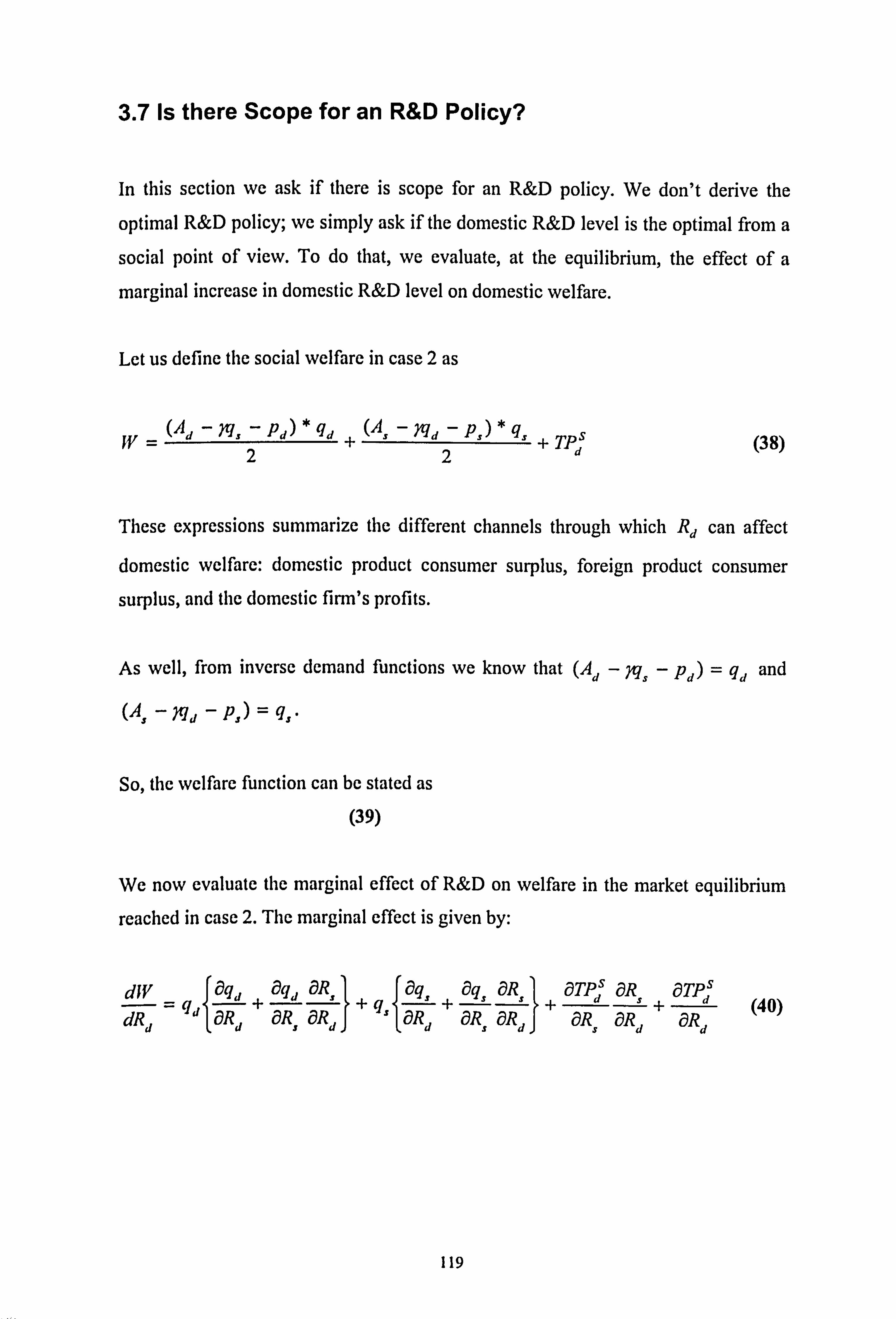
3.7 Is there Scope for an R&D Policy?
In this section we ask if there is scope for an R&D policy. We don't derive the
optimal R&D policy; we simply ask if the domestic R&D level is the optimal from a
social point of view. To do that, we evaluate, at the equilibrium, the effect of a
marginal increase in domestic R&D level on domestic welfare.
Let us define the social welfare in case 2 as
pd) *q (A., - Yqd - p, ) * q, d 1, d+
22+ Tpd (38)
These expressions summarize the different channels through which Rd can affect
domestic welfare: domestic product consumer surplus, foreign product consumer
surplus, and the domestic firm's profits.
As well, from inverse demand functions we know that (Ad Pd) =qd and
(A, - Nd - p, ) = q,.
So, the welfare function can be stated as (39)
We now evaluate the marginal effect of R&D on welfare in the market equilibrium
reached in case 2. The marginal effect is given by:
? q., +
Dqs ÖR +
DT d+ '3Td diV
=q1 d9q d.
aqd aRs sPs
öR, ps dR
- -" I OR. dR dR. I-I dR. i9R i9R
-I t9R V ;W -- L---a ijL ---dj ---s --'d -- (40)
119

aTPS Because we are evaluating welfare in the optimum, we have that
aR '=0, then d
dW f aq aq, aR I aq, +
aq, aR T: p s aR -=q dl
a_ _ -L + q., + dR aR aR., iFR. M aR., OR Ms 'R dddddd
(41)
The last term represents the profit shifting strategic effect of domestic R&D. The
other terms show the effect on surplus that domestic consumers derive from
consumption of the domestic and foreign product. Therefore, there are three basic
channels through which domestic welfare can be affected with a marginal increase in
domestic R&D.
As well, by using A=q, / qd eq. 44 becomes
dW aq d+ Lqd aR., aq, +
aq, aR', Ts aR. qd+d
d aRs aR d aR d aRs aR d+ dRd aR aR, t9R d
Note that
Oms = _(I _Y2 )2qd y +aRd 't or< 0
aR,
ý
(I _Y2 )(4 _Y2)ý
aR, _y(2
-y 2)
<0 aR dD
aqd (2 _ Y2)_ >0
aRd (I _ y2 )(4 _ y2)
aqd y 7<0
aRs (I _ Y2 )(4-
aq, =y aR
d (I - r2)(4
aq, =
(2 _ Y2)
aRs (I - y)(4 - y") ý>
0
(42)
In summary, the first term in equation 41 is positive since domestic product
consumer surplus increases, the second term is negative since subsidiary product
120

consumer surplus decreases and, as a consequence, the relative magnitude of these
two effects depends on the degree of product differentiation and the relative size of domestic and subsidiary product market size. On the other hand, the last term can be
positive or negative, since it depends on the relative effect of the subsidiary's R&D
on the domestic firm's profits, which implies that the profit shifting can call either for a subsidy or a tax on domestic R&D.
All these partial effects decrease when the degree of product differentiation. In
particular, if y -> 0, then aRS
=0 and dW
-> qdI>0. Therefore, if products aR d
dR d
ý21
are not related, a marginal increase in domestic R&D is welfare improving. On the
other hand, if y>0, in addition to the positive effect on the domestic product
surplus, we have a negative effect on the subsidiary's product consumer surplus, so
the relative market size of both products becomes relevant to the evaluation. The
higher the relative size of the subsidiary's market, the lower the increase in overall
consumer surplus. As well, we have a positive effect on the domestic firm's profits.
In summary, the net effect depends on the relative size of domestic and subsidiary
markets, the degree of product differentiation and the magnitude of the rent shifting
profits motive. This analysis must be taken as a preliminary step toward a more
complete analysis of the policy implications of the model developed in this chapter. However, results in this section suggests that the optimal level of R&D chosen by the
domestic firm couldn't be optimal. Hence, it suggests that there could be space for an R&D policy. Further research should analyse the optimal policy within the context of
this model.
121

3.8 Main Conclusions and Suggestions for Further Research
in this chapter we analyse FDI in less developed countries in which both the mode of
foreign expansion and the incentives to innovate are endogenously determined. This
is the main contribution of the model developed in this chapter since, to the best of
our knowledge; it is the first model that analyses FDI in developing countries with a
model of these characteristics. Our main objective is to shed some light on the impact
of the different modes, which a foreign firm has to reach a domestic market, on the
incentives to innovate and on the host country welfare.
We analyse a three-stage game in which the foreign firm chooses the mode of
serving the domestic market in the first stage. Then, in stages two and three firms
simultaneously choose R&D and price level, respectively.
Some key features of our analysis are:
We consider asymmetric R&D spillovers, which are received by the domestic
firm from the MNC when it decides to serve the domestic market by creating a
wholly owned subsidiary and undertakes R&D in the host economy. So
spillovers are geographically localized.
As well, we include in the analysis the idea that the degree of spillover received by the domestic firm depends positively on its own R&D effort, which incorporates the idea that the degree of R&D spillover depends on the absorptive
capacity of the firm that receives them.
R&D investment can be interpreted as aimed at either improving product quality
or reducing production cost.
The main issues and results are:
1) First, on the impact of the different market structures on the incentives to
innovate. We have shown that:
a) Provided the degree of spillover is small enough, when the foreign firm
moves from exporting to FDI, domestic and foreign firm R&D levels
decrease and increase, respectively.
122

b) Independent of the degree of spillover, total R&D increases. If the degree of
spillover rises, then total R&D increases further.
2) Second, on the preferred mode of entry of the foreign firm from the host
country's point of view.
a) If the foreign firm chooses FDI, provided the relation between foreign and domestic output is greater than one, consumer welfare increases while domestic output drops. If the degree of spillover increases it is possible that
domestic welfare increases, but also the foreign firm could be induced to
choose exporting. On the other hand, if the degree of product substitutability falls. Then it is more likely that domestic welfare increases. In the extreme
case that y=0 and a>0, then domestic welfare increases and therefore the
preferred mode of entry from the host country point of view is FDL
3) Third, on the determinants of the optimal mode of entry of the foreign firm from
its point of view.
a) The key determinants of the optimal mode of serving the host economy are:
the level protection of the domestic market, the degree of product
substitutability, the level of the plant specific cost and the degree of spillover. The higher is the first determinant and the lower are the other three; then the
more likely it is that the foreign firm will choose setting up a subsidiary. 4) Fourth, to determine if there is scope for a domestic R&D policy
a) Ours results suggest that there is space for a domestic R&D policy. The
optimal policy however requires further research.
Some policy implications are:
1. Host country governments must pay attention to domestic firms if they want to
improve the benefits received from FDL
2. To improve the benefits of R&D, we require strengthening absorptive capacity.
Finally, further research should be aimed at finding the optimal policy from the host
country's point of view.
123
Chapter 4
Research Joint Ventures in Oligopoly Markets
with Presence of Multinational Corporations
4.1 Introduction
This Chapter investigates research joint ventures (RJVs hereafter) in a duopoly
market with R&D spillovers and the presence of a MNC's subsidiary. This chapter is
a natural extension of the analysis undertaken in chapter 3. This takes into account
that RJVs are a form of collaboration that can be improve welfare under certain
circumstances, where the existence of R&D spillovers plays a central role. As well,
cooperation at the R&D level is increasingly common globally.
As a consequence, we keep the basic structure of the model developed in chapter 3
and extend it to analyse the case of R&D cooperation. As in the previous chapter, the
effects of successful R&D is to increase the firm's market size, either by improving
product quality (product R&D) or by reducing marginal production costs (process
R&D). Consequently, in this way we can generalise the way in which we model
R&D investment.
We consider a local market for a differentiated product where there is a competing
domestic firin, which produces only for domestic consumption, and a foreign firm
that is a MNC's subsidiary. The firms compete over two periods by choosing R&D
in the first and prices in the second (Bertrand competition). As usual, the firms'
problem is solved as a dynamic game of complete, but imperfect information. The
solution concept is subgame perfect equilibrium.
The model developed in this chapter falls into the literature on RJVs within the
context of strategic R&D with spillovers, which is surveyed in chapter 3. Another
key feature in our model is that we model R&D spillovers assuming that the firms'
capacities to absorb the knowledge created by other firms depend on their own R&D
124

efforts. In particular, the higher the R&D undertaken by a firm, the higher its ability
to receive R&D spillovers. Consequently, in contrast to most of the literature, we
explicitly consider the absorption capacity as a determinant of the ability to receive
R&D spillovers.
We analysc four different cases, in all of which the firms compete in a Bertrand
fashion in the second stage. In the first stage, however, we allow both the possibility
that firms coordinate their decisions on R&D in such a way as to maximise the sum
of their first stage profits, and that firms receive R&D spillovers. The four cases
considered are:
I. Firms compete in both stages and there are no R&D spillovers
2. Finns make a joint decision on R&D, compete in the product stage and there are
no R&D spillovers
3. Firms compete in both stages and there are R&D spillovers
4. Firms make a joint decision on R&D, compete in the product stage and there are
R&D spillovers.
We focus our analysis on the equilibrium R&D levels under the different cases
considered and see how it depends on the degree of product substitutability, the
degree of R&D spillover and the relative sizes of the markets faced by the firms. As
well, we undertake welfare analysis and establish the condition under which host
countries should allow RJVs.
This chapter is organised in 7 sections. In section 4.2 we set up the model and solve
it for the production (second) stage. Then, in section 4.3 we solve the R&D (first)
stage of the model in the case that there are no R&D spillovers. In section 4.4 we
solve again the R&D stage, but for the case of R&D spillovers. In section 4.5 we
undertake a comparison of the equilibrium R&D levels in the different cases
considered. Section 4.6 analyses the impact on domestic welfare. Finally, in section
4.7 we conclude by providing some policy implications and suggesting further
research.
125

4.2 The Model
We keep the basic structure of the model developed in chapter 4 to analyse here the
case of the firms' co-operative behaviour in the R&D stage. This structure can be
summarised as: 1. In the context of a two stage strategic R&D, a domestic firm and foreign firm
compete by simultaneously choosing an R&D level and prices in stages one
and two, respectively.
2. On the demand side, both firms produce a horizontally differentiated product. 3. On the production cost side, both firms face a constant marginal cost
function.
4. The firms invest in R&D with the aim of improving product quality with an R&D cost function that exhibits marginal increasing cost. Details on R&D
cost functions will follow below.
The specific details of this co-operation will be explained below. On the other hand,
during the second stage firms will continue behaving non-co-operatively in a Bertrand fashion, as in chapter 4.
4.2.1 Second Stage Firms'Problem
We start by solving the second stage fin-ns' problem. At this stage both firms make a decision on their prices simultaneously, in a non-co-operative way, taking as given
the R&D levels chosen in the first stage.
Let the two firms and goods be labelled d (domestic) and f (foreign). All other
notations are as in chapter 4, from which we know that the demand functions faced
by the domestic and foreign firms are, respectively
qd ý- [ 7- 71]lAd - PA - y[Af - pf
ý (1
126

qf = 11
-172
fAf - Pf
I- YlAd - Pdll (ib)
The parameter y (0 <y< 1) reflects the degree of product differentiation. The
lowest degree of product differentiation is reached when y -> 1, which is the case
when products become homogeneous. If y decreases, the products become more
differentiated. The extreme case is when y -> 0, which is the case where products
become unrelated. Evidently, in the latter case, demand functions converge to
q, = [A,
- p, j and therefore, each f inn is a monopoly in its own variety.
As mentioned above, in the second (production) stage, firms compete in prices. As a
consequence, the second period equilibrium involves
Max Pi
Cd 1'.
1 d- Pdl - r[Af - Pf (2a)
Maxpf Irf -, ý lpf
-ftI ul
f- Pf I-
YlAd - Pdl (2b)
The best response function for firms I and 2 are, respeCtiVel 4
Pd =I 1'4d
+ Cd - y[. 4f - pf 2
-ý I fAf
+ Cf -y [Ad
- Pd Pf '" 2
(3a)
(3b)
Note that dp, / dpj = (y / 2) > 0, i=d, f, j=d, f, d;, - f. Therefore, prices are
strategic complements. As a stability condition, we require that Idp, / dpj I< 145 be
satisfied for both firms. These conditions are met because 0<y<1, which implies
that dp, / dp, is positive but lower than 1/2. Note that the slope of best response
' Second order condition requires y2)> or Y2 <>Y< Consequently, the s. o. c. is
always satisfied. 45 See Henriques 0 990) for details.
127

functions depends on the degree of product differentiation. In particular, dp, / dpj -+ 0 when the products become more differentiated or unrelated (y -4 0 ).
By solving best response functions, we find the equilibrium prices, which are
Pd 12 12
-y2 ]A
d+ 2cd - y[Af - cf 4y
PA --2
12 -y2
ýf + 2cf - Y[A d-cd f4y
(4a)
(4b)
Hence, for firm i U=dJ), its equilibrium price is higher the higher its own product
quality level (A, ), its own marginal production cost (c, ), the other firm's marginal
production cost (c) and the lower the other firm's product quality level (A). Note
that the equilibrium price functions are independent of the type of competition
undertaken by the firms during the R&D stage. However, the price equilibrium level
can differ because, as we will see later, it depends on the R&D equilibrium levels,
which in turn depends on the type and degree of competition or collaboration in the
R&D stage.
We can solve for I (2[A Ad - Pd : -- T- d-
Cdl + Y[Af - Cf (5a)
AI- Cf I+
YlAd - Cdll (5b) f- Pf ý-- T-_
Y2
(2[Af
Further
qd y2
I_
Y2)
12 _ Y21A d- Cdl - YlAf - Cf
1
)(4 (6a)
qf r2
I_
r2)
]12
_ r2JA f-
Cf I-
YlAd - Cdll (6b) )(4
and
128

12 _ 72
JA -C- Y[A (7a) Pd - Cd 4y2d dl f -CfD -
Pf - Cf Y2
12_ Y21.4 f- Cf
I- 714d - Cd
11 (7b)
The interesting feature of these solutions is that we can think of A.. - c.. as
measuring the market "size" for goodj, and the key variables for the profits of each firm are then the market sizes of the two goods and the degree of substitutability between them (y). For instance, for equations (7a) and (7b), the endogenous
variable becomes the margin price-unit production cost, which is higher, the higher
the market size for its own variety and the lower the other firm's market size.
Note that (p, - c, ) -> [-I ] jAj
- c, D if 0, a case in which each finn converges 2
to be a monopoly in its own variety. As well, as long y increases, which happens
when the products becomes less differentiated, then (p, - c, ) decreases.
Let M, = Aj - c, . Then, we can gencralise the previous results (i. e. the results in
the previous chapter with horizontal differentiation) by assuming that the effects of
successful R&D by f inn i is to increase its market size, either by improving product
quality (A, ) or by reducing marginal cost (c, ). There is no particular need to
differentiate between the two.
Note that given the equilibrium prices in stage 2, a necessary condition for qd ý! 0
(equation 6a) is that 2)Md
_ Mf [(2 -yy
]> 0.
Let us define A= (Aff / Md) as the relative size of the foreign firm's basic market in
relation to the domestic firm's basic market, which implies that Mf = AMd.
129

The previous condition implies that equation (8) can be expressed as [_ 72) _ A]"d >0 [(2
_ Y2) _ A]> 0>A< [(2 _ V2 Y]. (2 YY
Consequently, there is a maximum relative size of the foreign market such that the
domestic firm has a positive demand. The reason is that given a relative market size (A), the negative effect of firm'sj market size on firm's i profits is higher the more
homogenous are the goods. Hence, the lower is y, the higher is the relative size of
the foreign firm's basic market, which is compatible with the domestic firm facing a
positive demand. The following table shows the maximum value for A for different
degrees of product substitutability (y). We can see from table I that the maximum
value for A increases as product differentiation increases. For instance, if y=0.5 , the maximum value for A is 3.5, so the basic foreign market can be at most 3.5 times
the size of the domestic market, otherwise the demand faced by the domestic firm is
zero.
Table 1 y A 1 1,00
0,9 1,32 0,8 1,70 0,7 2,16 0,6 2,73 0.5 3.50 0.4 4,60 0.3 6,37 0,2 9,80 O'l 19,90
0,01 199,99
We will now analyse the first stage firms' problem considering four different cases:
1. Finns compete in both stages and there are no R&D spillovers. This is the full
non-co-operative case.
2. Finns make a joint decision on R&D, compete in the product stage and there are
no R&D spillovers.
3. Firms compete in both stages and there are R&D spillovers
4. Firms make a joint decision on R&D, compete in the product stage and there are R&D spillovers.
130

From now on we will call these four different scenarios cases 1,2,3 and 4,
respectively. In cases 2 and 4, firms choose their R&D levels to maximise the sum of
their first period profits. Consequently, we will not consider the full co-operative
case in which the firms co-ordinate their decisions in both stages of the game (R&D
levels and prices). Consequently, under the RJV agreement that we consider, the
firms co-ordinate their R&D expenditures in such a way to internalise the impact of
the other firm's R&D level on its own profits, which is negative in the case of no R&D spillovers and can be positive or negative in the case of R&D spillovers.
131

4.3 The Model without R&D Spillovers
Let us to take the case of no R&D spillovers in the first instance. We therefore can
write
M, + R, (9)
where M, is what firin i's market size would be if it conducted no R&D. We will
call this its "basic" market. Note that this basic market is higher the higher is the
initial firm's product quality and tile lower is the firm's initial unit production cost.
Note that from equations (6a) to (7b) it follows that for firm j (i = d, J)
qj = [I /(I - y')Ipj - c). Consequently, in the first stage, profits can be expressed
either as
(pj - c, )q, - C(Rj) =1 )2
- C(R T-7 (Pi - ci, or
(10a)
(pj - c, )q, - C(Rj) == (I _ Y2 )q 2- C(Rj) (10b) j
where C(R) is firmj's R&D cost function.
Tile costs of R&D are assumed to be C(Rj) =R2 and therefore exhibit increasing i
R&D marginal cost. In other words, the cost of increasing the market size of firmj
by one unit is higher the higher is its own R&D level.
4.3.1 Case 1: Non Co-operative Equilibrium and No R&D Spillovers
In this case firms compete in both stages. Therefore, the firms' first period profit
maximisation problem becomes
132

Max ;T12 IjWd
+R +Rfr -R 2
Rj d 214 -12- y d] - Y[Hf d 11
-y- Y2]2
Max Rf 12
-y2 IR
+R ]- y[jWd + Rd]ý -
R2 11-7 214
_ Y2]2 fff
which gives the best response function of
- yRf I
Rf LD_
y2]T - Y, - YA 2- Y" 12 If Ald ýRd
Rd=D 12-7 2 ]; W d_ YM7-f
r 11
(11 a)
(lib)
where D= [I - y'I4 - y'll -
[2 -, v'12, which needs to be positive for both R&D
levels to be positive. As well, this is the second order condition. By using numerical
methods I found that to have D>O, we require that y :: ý 0.94. Consequently, the only
restriction is that products cannot be too homogeneous.
Note that A,
=- (2 _ Y2)y
< 0, which implies that in this case R&D levels are Aj D
strategic substitutes. The reason is that firin i's R&D exerts a negative effect on firm
j's profits by reducing the demand of its product and therefore the incentives to
undertake R&D. It can also be thought of as a negative externality.
To have a stable equilibrium we require that JdR, I dRjj < 1, which means
1(2 - Y2 )y]l D) < 1. This condition is satisfied if y :50.88, so this means that we
require a more stringent condition on the degree of product differentiation: products
need to be more differentiated than is required to satisfy the second order conditions.
The two response functions can then be solved for the equilibrium R&D levels in
case 1, which are
133

Rl =[ [2
_ Y2]
2
]J2
_Y2 ID + y2]ýWd - y(D + [2_ Y2]2),
g I
(12a) dD2_y2 [2 -y21f
Rf' = [2
-y21 ]12
_ Y2 ID + Y2]ýWf - v(D + [2 _ 72]2)jWd) (12b)
[D
2_y2 [2 -y2f
Note that in the previous two equations the difference between the foreign and
domestic equilibrium R&D levels is
R fl - Rlj -- [2
-y2 1-
12 - yjl + y]D + y[2 -y2
11 _ YJ2 + Y]JO _
Rd]. [D
2_y 2[2 _ Y2
121f
Obviously if market sizes are the same, so are equilibrium R&Ds. Otherwise the firm
with the larger basic market undertakes more R&D than the other firm. On the other hand, the magnitude of the difference depends on the degree of product
substitutability.
134

4.3.2 Case 2: Co-operative Equilibrium and No R&D
Spillovers
The above is the competitive solution when firms choose their R&D investments,
taking that of the other firm as given. This is now contrasted with the case where the
firms make a joint decision on R&D - but still compete in prices in the second
period. Such Research Joint Ventures (RJVs) are permitted, and are often justified on
the grounds of spillovers in R&D among firms. Our interest here is to see their
effects when there are no spillovers (spillovers will be allowed below).
The RJV will choose the R&Ds of the two firms to maximise the sum of their first
period profits. These prof-its take into account that the two firms will be Bertrand
competitors in the output markets in period 2. So it is not the ftill collusive outcome,
a case in which firms coordinate their decisions in both stages. We will consider only
the case of RJVs because it seems to be more relevant, taking into account that to
coordinate decisions to the product stage are allowed. Hence, the type of RJV we are
considering implies that the first period decision will now take into account the
negative externality that each firni's R&D imposes on its rival. The RJV will then
jVfar,,,,,; r = ; rd + ; r, I
Y214
12-Y 2 Jýqd +R dl - Y[Hf + Rf r
Y2 ]2
1+
12 _ Y2
I; Wf + Rf ]- y[jWd +Rd
IY } JR2
+R2 df
The first order condition for R, then gives us the reaction functions 46
12 IN-
_ Y2 ]Uf
_ Y2 ýf )
Rd = [D-y
2
](12-y2]1+y 'fd-2y[2 - 2y[2 (13a)
46 Second order conditions require that I(I
- y2)(4 - Y2)2 -(2 _ y2)2 I-y 21 =
[D _ Y2] ý:. 0.
This condition, which is morc stringent than for case 1, is satisfied for y :50.88.
135

Rf =[ 1 112-7 22+ Y2 2y[2 -, v 2 jHd
- 2y[2 _72 D-Y 21 (13b)
By solving equations (13a) and (13b) we obtain the equilibrium values for R&D in
case 2, which are
]fl2-y 2 ]2 [D
+3 Y2 1
+7 2 [D_y2 - 2
Iýld
Rd [D
-72 ]2
-4y2[2 _ Y2 ]2 jj- 27[2 -y2
RD+(2 _72)2
ljwf
R2=[1 Y2 _r2]2
]fl2-y 2 ]2 [D
+ 3y2 + 72 [D_72 twf
_ Y2 ]2
_y2lD+ V2)2 )Rd f [D
-4 [2 2y[2 (2 _,
22 We are now in a position to compare Rf - Rd
(14a)
(14b)
[(2 -y
2)2 [D + 372
2 ]2 Y2[2 _ 72
]2 +7 2 [D
-7 21
[D -Y -4
1-2,
v [2
_ V2RD + (2 -y 2)2
R=
136

4.4 The Model with R&D Spillovers
Now we introduce R&D spillovers between firms. The simplest way to do this in this
context is to introduce them as was done in the previous chapter - through the cost Of R&D. The idea here is that each firm can benefit from its rival's R&D, but only if it
conducts R&D itself. In other words, we model R&D spillovers on the assumption
that the firm's capacity to absorb the knowledge created by other firms depends on its own R&D effort. Hence, the higher is the R&D undertaken by a firm, the higher is
its ability to receive R&D spillovers. This is in line with the ideas developed initially
by (among others) Cohen and Levinthal (1989) and then introduced formally in a
strategic R&D model by Kamien and Zang (2000).
Thus,
C(R, ) = R, [R, - pRj
I=R12- pR, Rj (15)
where p, with I 'zý p ý: 0, denotes the "spillover" parameter. Then firm i's R&D
costs are zero in two circumstances, first if it conducts no R&D itself (i. e. Ri = 0)
and, second, when its R&D exactlY matches the knowledge spillover from the other
firm's R&D (i. e. R, = pRj).
4.4.1 Case 3: Non Co-operative Equilibrium with R&D Spillovers
Now we solve for non-co-operative equilibrium in R&Ds with spillovers. The
maximisation problem for both firms is
Max z -,: [1 1 12
-y2 IjWd
+R- y[jWf + Rf [R2 _R Rd d
Y214_ Y2]2 dl d PRd
f]
I_V2 IjWf
_[R2 Max ;r "ý Ft --2L
12 12
+ Rf ]- y[jWd+ Rdtf- pRfR 7ý12 R, f --2 -dI Rf "f- 11
-r 214_
Y2]2
137

which gives the following best response functions 47
Rd 1 ý[2-r 2 ]2 jWd
- 2y(2 _y2 )jWf +D, Rf
2D
Rf ý[2_y2]2jqf
-2y(2-r 2 )Md+D, Rd
2D
where D, = p[l -r 214_
72]2 - 2y[2- r 2]
(16a)
(16b)
Note that one firm's R&D will be independent of the other's if the spillover
parameter takes on the critical value
11-7 214_ Y2]2
if p> ;5 the two R&Ds are strategic complements, otherwise they are strategic
substitutes. Hence, the existence of the spillover, if it is sufficiently large, can change
the nature of the R&D game. The critical value depends on the degree of
substitutability between the products (y). By using numerical methods we find that
the critical p is lower, the higher is the degree of product substitutability (lower y).
Consequently, ;3 is higher, the more homogenous are the products. As well, we
found that the critical value (; 5) increases from 0 when y=0 to I when y=0.89.
Further, it implies that the possibility that R&Ds becomes strategic complements is
higher, the higher is the products substitutability.
Notice that in this case, in addition to the negative effect that firm i's R&D level
exerts on firm j's R&D, there is another effect that exerts a positive effect. Notice
that this negative effect is higher, the lower is the degree of product substitutability (the higher is r ). This is the effect of the R&D spillover, which reduces the marginal
cost of R&D and therefore increases the incentives to undertake R&D investment.
What effect predominates deten-nines the strategic effect of one firm's R&D on the
47 The second order conditions require D= 11 - Y'14 - y'f -
[2 - y'f > 0, which is satisfied if
y :50.93.
7ý - 2y [2
_ 721
138

other. The higher is the degree of spillovers and the higher the degree of product
substitutability implies the more likely it is that R&D levels be strategic
complements.
The equilibrium R&D levels are
R3 2(2 _ 2,2L 12(2
_Y2 )D - yD, ]Rd
- [2yD
- (2 _72 )DI (17a) d (4D 2-D, 2)
R3 2(2 _ Y22_ 12(2
_Y2 )D - ýDj ]ýWf
- [2yD
- (2 _ V2 )DI ]Rd
f (4D 2 -D,
2) (17b)
Note that if p -> 0 then, D, -> -2y(2 - y).
- .. -3 - 2(2 _ Y2)
[[2(2 _Y2 )D +2 Y2 (2 _ Y2)
Purtner Ký (4D 2
-4 y2 (2 _ y2)2) J_ [2yD
+ 2y(2 _ Y2)
(2 _ Y2) [(2
-y 2) [D +y
2pd
(D 2 _Y2 (2 _ Y2)2) -r
[D + (2 _ 72)2pf
Rd I
I d
In effect, the domestic equilibrium R&D level in cases I and 3 are the same if
p=0, a result that is quite intuitive considering that the only difference between
both cases is that case 3 considers the existence of R&D spillovers.
139

4.4.2 Case 4: Co-operative Equilibrium with R&D Spillovers
We will now consider the case of cooperative equilibrium in the presence of R&D
spillovers. The potential existence of the R&D spillovers has been used to argue the
case for allowing firms to form a RJV in such circumstances. The argument is that
the RJV will lead both firms to intemalise the existence of spillovers and therefore to
undertake greater R&D than they would if they acted non-co-operatively. This will
now be investigated. The optimisation problem for the RJV is
Max Z=Z +; r =11
12_ Y21Hd +R dI- rljWf + Rf r
df 214 _ V2]2 _ Y21Hf
11 -y +12 + Rf ]- y[Rd +Rd
IY
- [R 2+R2
-2pR R dfd f]
The first order condition for both firm's R&D provides us with the reaction
functionS48
Rd ýý [D
y2
112 -22+y2 2y[2 - y2
]2Wf + DjRf (18a)
Rf =[ Dy2 ý12
-y22+y2 2y[2 _ Y2 ]ýWd
+ DIRd (18b)
Note that if p=0 then D, = -2y(2 -y2) and, therefore, the R&D reaction
functions become the same as in case 2, RJV with no R&D spillovers. In that case
the equilibrium R&D level would be the same in cases 2 and 4 (R 2=R 4). dd
For the RJV, the R&Ds of the two firms are "independent" if the coefficient on R2 in
this expression is zero. That is, if
48 As in case 2, the second order conditions require that 10
-y 2)(4
_ Y2)2 -(2 _ Y2)2 2
y2 0. This condition is satisfied for y
y :50.88.
140

2y[2 _ r2]
Y214_ V2]2 jo
Again, if p<3, the R&D levels are strategic substitutes. On the other hand, if
p> ; 3, the R&Ds are strategic complements.
The equilibrium R&D levels are
I ]f J(D _ V2 )[(2 _y2)2 +Y2 J-2y(2 _Y2 )DI jHd
r-r-- -'R- .
R=[
I
(D-y 2)2 - D, 2 [2y(D
_Y2 )(2 _y2)_ D, [(2 _y2)2 +y2]Uf
I J(D -y2 )[(2 -r
2)2 +Y2 I-
2, v(2 _Y2 )DI JHf
(D -y
2)2 -D2
[2, v (D _Y2 )(2 _Y2 )-D, 1(2-y 2 )2 + r2
jUd
I
(19a)
(19b)
As well, if p -+ 0, then D -27(2 -72) and therefore R4 -> R2. The dd
equilibrium R&D level in cases 4 and 2 are the same if there are no R&D spillovers.
141

4.5 Comparison of Equilibrium R&D Levels
Now we will compare the R&D levels under the different scenarios. First, remember
that A=jWf IRd is the relative size of the basic foreign market in relation to the
basic domestic market. Obviously, provided that both basic markets are positive, A>0. As well, if A>I (A < 1), then the basic foreign market is bigger (smaller)
than the basic domestic market. The definition of A also implies that AMd = Mf
Let us also define R' as the equilibrium R&D level undertaken by the domestic firm d
in case i (i=1,2,3 and 4), which are
Rd' =[ [2
-y2 ]J2
-y 21D + Y2]; Wd
- y(D + [2 _ Y2]2)jWf (12a)
D2_y 2[2 _ r2]2
] 12-y 2 ]2 [D
+3 72]+y2[D_y2 -
R2= ]ý-ld
(14a) d [D -y2
J2 -4y2[2_ Y2
]2
- 2y[2 - y2RD + (2 _ 72)2 JHf
R3 2(2 _ Y22_ J2(2
_ ;, 2 )D - ýDj ]ýWd
- [2yD
- (2 _ V2 )DI d (4D 2 -D,
2) luf I (17a)
R4 =[ I.
J(D _Y2 )[(2 _y2)2 +72 ]-2y(2
_Y2 )DI )Hd
(19a) d (D _ 72)2 - D, 2-- [2y(D
_Y2 )(2 _Y2) - D, [(2 _y2)2 +y2]Uf
I
Note that if p=0 and y=0, then D, =0 and D= 12, which implies that
Rd' = Rd =3d = R' = (I / 3) -. Hence, with products that are not related (y = 0) and d Ald
with no R&D spillovers (p = 0) the domestic firm (and foreign of course) undertake
the same R&D level in equilibrium in cases I to 4.
Let us now consider the case that y>0. From the previous sections we know that if
P=O, thenR' =R' and R4= R'. Let us see what happens with the previous two dddd
142

equalities when p increases. First, from the best response functions in cases 2 and 4,
equations (I 6a) and (I 8a), respectively, we know that
Ad= jD + (2 -Y R >0 and dp 2D f]
dRd [D + (2 _ V2j
Rf dp D-y 2 >0
Then, for any given R&D level of the foreign firm, if p increases the domestic
firm's R&D expenditure increases. It also happens with the foreign firm's best
response function. Consequently, if p>0, the R&Ds equilibrium levels increase. In
particular, for a given y>0 they are higher, the higher is the degree of spillovers.
Therefore, we can conclude that for a given y ý: 0 and p>0, then R' > R, and dd
R' > R'. As well, the difference between the equilibrium R&D levels increases as dd
does p, because it decreases the marginal cost (increases the marginal benefit) of the
R&D expenditure.
Let us now consider the effect of the degree of product substitutability (7) for a
given degree of spillover (p). To make this comparison we will make some
numerical simulations. Note that if we introduce the relation Ajw, = Hf into the
equilibrium domestic R&D level, then equations (12a), (14a), (17a) and (19a)
become
Rd' =[ [2
_y2 1-]12
-y 21D + 72]_ y(D + [2
_ Y2]2 )A (20) D2y2 [2
y212
)Hd
R2=[2 J2
1
Y2[2
If 12 -r2
]2 [D
+3 Y2]+ r2[D_ ), 2 1
(21) d [D -y -4 _ Y2]2 ] [- 2y[2 _Y2RD + (2 _ V2)2
ý Hd
R3- 2(2 _ 72) 12(2
_Y2 )D -ýDj- [2yD
- (2 _Y2 )D d (4D 2-D1 2) 1
ýwd
(22)
143

4 J(D
_ Y2 )[(2 _ Y2)2 + Y2 2y(2 _ Y2)DI 41 Rd (D
-y 2y
_D 12 - [2y(D
_ Y2 )(2 _ Y2) - D, [(2 - Y2)2 + Y2]ý
'Ud (23)
In these specifications, equilibrium domestic R&D levels depend on their basic
market, the degree of product substitutability and the relative sizes of basic markets
(A). Consequently, the R' can be expressed as d
=KM 1
where K, depends on the parameters ; v, p and A.
Let us compare first the equilibrium R&D levels in cases I and 2 (so p= 0). As we 2
know, if y=0, then Rd' =Rd. As well, if y increases, then both K, and K2
decrease and, as a consequence, for any given jWd, R' and R2 also do the same. dd
The reason is that when y>0, the other firm's R&D exerts a negative effect on
domestic profits and, therefore, reduces the incentives to undertake R&D. This
effect, however, is interrialised when firms coordinate their decisions on R&D and,
therefore, their R&D levels are lower than in case I when y increases. This can be
seen by observing in table 2 that K, decreases when y increases, but K2 decreases
faster than K,. This implies that for a given p and A when y increases then
Rd' >R2 and the difference increases monotonically as y is higher. d
Note in table 2 that, since p=0, then K3 = KI and K4=K2 and, as a
consequence, Rd' = R' and Rd' = Rd. As well, we can observe that K-K and d12
K=K increases as r does, implying that R2- R1 and R3- R' also increases. 34dddd
43 A similar line of reasoning can be made to show that if y=0, then Rd>Rd. In
fact, the highest domestic R&D level is reached for a given A when r=0 and
p>0. As well, the difference R4- R' increases as p does. If y increases then dd
144

R4 decreases faster than R' and therefore for ay great enough, R4- R' can dddd
become negative.
Table 2
and P0 KI-K2 K3-K,
K, K2 K3 K4 K3'K4 K4-K2 0,00 0,333 0,333 0,333 0,333 0,000 0 0,04 0,325 0,316 0,325 0,316 0,009 0 0,08 0,317 0,301 0,317 0,301 0,017 0 0,12 0,310 0,286 0,310 0,286 0,024 0 0.16 0,303 0,272 0,303 0,272 0,031 0 0,18 0,300 0,265 0,300 0,265 0,035 0 0,22 0,294 0,253 0,294 0,253 0,042 0 0,26 0,289 0,241 0,289 0,241 0,048 0 0,30 0,284 0,229 0,284 0,229 0,055 0 0,34 0,279 0,218 0,279 0,218 0,061 0 0,38 0,274 0,207 0,274 0,207 0,068 0 0,42 0,270 0,196 0,270 0,196 0,074 0 0,46 0,266 0,185 0,266 0,185 0,081 0 0.50 0,262 0,174 0,262 0,174 0,088 0 0,54 0,258 0,163 0,258 0,163 0,095 0 0,58 0,254 0,152 0,254 0,152 0,102 0 0,62 0,250 0,140 0,250 0,140 0,109 0 0,66 0,246 0,129 0,246 0,129 0,117 0 0.70 0,242 0,117 0,242 0,117 0,125 0 0,74 0,237 0,104 0,237 0,104 0,134 0 0,78 0,233 0,091 0,233 0,091 0,142 0 0,82 0,228 0,076 0,228 0,076 0,152 0 0,86 0,223 0,061 0,223 0,061 0,161 0 0.88 0,220 1 0,054 1 0,220 1 0,054 1 0,167 0
In summary, we have thatfor a given A, if p>0, y>0 and r is not too great
R432 d>Rd> Rdl >Rd. On the other handfor a given A, if
jo > 0, r>0 and v is
great enough, then R3>R4 >Rl >R 2
dddd
145

4.6 Welfare Analysis
The central aim of this section is to analyse the impact of the different types of RJVs
on the domestic welfare. In particular, we are interested in the conditions under
which the host country should favour RJVs.
Consumer Welfare
As explained above, the effect of successful R&D is to increase the firm's market
size, either by improving product quality (product R&D) or by reducing marginal
production cost (process R&D). As well, from the equilibrium prices (eqs. 4a and 4b)
we can verify that
dpi (2 _ y2)
dA, (4 - y2)
dp, 2 dc, (4 _ Y2)
i=d, f
i=d, f
Both expressions, given the restriction on parameter 7, are greater than zero. As
well, the first expression is lower than 1/ 2 and the second is lower than 2/3. The
first case shows the impact on firm i's equilibrium price of an increase in product
quality (product R&D) and the second of a reduction in unit cost of production (process R&D). This result tells us that the benefits of R&D, either product or
process R&D, are shared by consumers and firms. Consequently, consumers get a higher surplus when R&D investment increases, independent of its type.
On the other hand, from the equilibrium outputs (eqs. 6a and 6b) we can show that
T=qd +qf Y2
1 (2-y2 -y)
Od
+ jWf + Rd + Rf )(4 - y2)]
where Q' is total output.
(24)
Equation 24 tells us that total output is higher, the higher are both the firm i's basic
market and R&D level. Hence, total output increases if total the R&D level also does
146

so. The other determinants of total output are the exogenous basic markets and the degree of product substitutability.
As well, from chapter 4 we know that domestic consumer welfare can be stated as
q2 +
qf2 CS =d
22
Hence, consumer surplus depends on the output levels of the domestic and foreign
product. As well, from equation 24 we know that output levels are higher, the higher
are R&D levels, which implies that given the basic market sizes and'V, exogenous
variables, consumer welfare depends only on the R&D levels. The reason for this
result is that when R&D increases, so also does consumer welfare as explained
above.
The previous result is very important because consumer surplus depends only on the
R&D levels, and from that we can infer that the preferred equilibrium from the
consumer's point of view is the one where the R&D levels are the highest.
R&D Levels
On the other hand, the R&D levels depend basically on the basic markets and the
degree of product substitutability. In particular, the firm with the higher basic market
undertakes more R&D than the other firm. As well, from section 5.5 we know that:
If there are no R&D spillovers, the R&D level is lower if RJVs are allowed,
compared with tile level reached with non co-operative equilibrium.
Consequently, a necessary condition to allow RJVs is the existence of R&D
spillovers. This is Rd' > Rd -
R&D levels in the presence of R&D spillovers are higher than R&D levels
without them. This is in true, independent whether or not RJVs are allowed. 42 This Rd > Rd' and Rd > Rd.
Notice, however that R&D spillovers are a necessary but not a sufficient
condition to allow RJVs, since the effect of firm i's R&D on firm i's profits depends on two opposite effects. First, a negative effect that follows from the
reduction in the marginal benefit of its own R&D, which is higher the less
147

differentiated are the products. Second, a positive effect caused by the
reduction in the marginal cost of its own R&D, which is higher, the higher is
the degree of spillover. Thus, if there are R&D spillovers and products are
sufficiently differentiated, then R4> R'. This is the case in which R&D dd
spillovers should be allowed. A necessary condition for this is:
P> 2y[2 - y']
11 -Y
214_y2]2
if this condition is met, then R&D levels transform into strategic
complements. In other words, a necessary condition to allow RJVs is that R&D levels behave as strategic complements.
On the other hand, if there are R&D spillovers but products are differentiated
enough, R&D levels are strategic substitutes and, as a consequence, R' >R4 dd
A necessary condition for this to happen is
2y[2 - r2 ]
"' - [I - y'14 -, v 2 J2
Notice that tile critical value for the degree of spillover is higher, the less
substitutes are the products.
Domestic Welfare
As a summary, we can conclude that domestic welfare is higher, the higher is the degree of spillover and the more differentiated are the products. The reason is that
under those conditions, the higher are the R&D levels, the higher are outputs, the domestic fimi's profits and domestic consumer surplus. As well, under these
conditions, provided the R&D levels are strategic complements, the host country
should allow RJVs agreements. The worst case is when there are no R&D spillovers
and finns are allowed to make RJVs. In that case, finns intemalise the negative
extemality of the other firm's R&D level and, therefore R&D levels decrease, output decreases and so also does consumer's surplus. Firm profits increases, but total
surplus does not.
148

4.7 Main Conclusions and Policy Implications
In this Chapter we have analysed RJVs in a duopoly market with R&D spillovers and
the presence of a foreign firm. A novel feature in our model is that we model R&D
spillovers as assuming that the firm's capacity to absorb the knowledge created by
other firms depends on its own R&D effort. As well, we generalise the way in which R&D investment is modelled by assuming that the effects of successful R&D is to
increase the firm's market size, either by improving product quality (product R&D)
or by reducing marginal production cost (process R&D).
We analyse four cases, which are:
I. Finns compete in both stages and there are no R&D spillovers
2. Firms make a joint decision on R&D, compete in the product stage and there
are no R&D sPillovers
3. Finns compete in both stages and there are R&D spillovers 4. Firms make a joint decision on R&D, compete in the product stage and there
are R&D spillovers.
The main results we obtained are
" The equilibrium R&D levels depend on the degree of product substitutability,
the degree of R&D spillover and the relative sizes of the markets faced by the
firms.
"A necessary, but not suflicient condition to allow RJVs should be the
existence of R&D spillovers.
" To allow RJVs, a sufficient and necessary condition is that R&D levels be
strategic complements, which requires the existence of R&D spillovers and a high degree of product substitutability.
" Consumer surplus depends only on the R&D levels. In particular, the higher
the R&D levels, the higher is consumer surplus. The reason is that R&D
investment, either aimed at improving product quality or reducing production
cost, generates a surplus which is shared both by the firm that invests in R&D
and consumers.
" The higher are the R&D levels, the higher is domestic welfare.
149
The worst case for the host country is to allow RJVs when there are no R&D
spillovers. Domestic welfare is higher, the higher is the degree of spillover and the more differentiated are the products.
There are a number of issues, however, that require further research. For instance,
since foreign firm profits do not enter into domestic welfare, it would be interesting
to find if there are strategic rent shifting policies. As well, the optimal policy taking
into account the domestic welfare is an open question. Finally, other types of
cooperation between firms should be analysed.
150
5. References
1. Amir, R. (2000), "Modelling Imperfectly Appropriable R&D via Spillovers".
Itilei-tiatioiiaIJoiti-iialofliiditsti-ialOi-gaiiization, Vol. 18, pp. 1013-1032.
2. Arrow, K. J. (1962), "Economic Welfare and the Allocation of Resources for Invention". In The Rate andDirection ofInventive Activity. Princeton: Princeton University Press.
3. Bagwel, K. and R. W. Staiger, (1994), "The Sensitivity of Strategic and Corrective R&D Policy in Oligopolistic Industries". Journal of International
Economics, Vol. 36, pp. 133-150.
4. Barrel, R. and N. Pain, (1997), "Foreign Direct Investment, Technological
Change, and Economic Growth within Europe", The Economic Journal, Vol. 107, pp. 1770-1786.
5. Barros, P. and L. Cabral, (2000), "Competing for Foreign Direct Investment".
Revien, ofInternational Economics, Vol. 8, pp. 3 60-37 1.
6. Blomstrom, M. and A. Kokko (1998), "Multinational Corporations and Spillovers". Journal ofEconomic Surveys, Vol. 12 (2), pp. 1-3 1.
7. Brander, J. and B. Spencer (1983), "Strategic Commitment with R&D: The Symmetric Case", The Bell Journal ofEconomics, Vol. 14 (1), pp. 225-235.
8. Campbell, N. and N. Vousden (2003), "Training and Technology Transfer". Australian Economic Papers, pp. 35-49.
9. Caves, R. E. (1996). Multinational Enteiprises and Economic Analysis. Cambridge University Press.
10. Choi, C. J. and Shin, H. S. (1992), "A Comment on a Model of Vertical Product Differentiation", Journal ofIndustrial Economics, Vol. 40, pp. 229-232.
11. Coe, D. and E. Helpman (1995), "International R&D Spillovers". European Economic Review, Vol. 39, pp. 859-887.
12. Coe, D., Helpman, E. and W, Hoffmaister (1999), "North-South R&D Spillovers". The Economic Journal, Vol. 107, pp. 13-49.
13. Cohen, W. and D. Levinthal, (1989), "Innovation and Learning: The Two Faces
of R&D". The Economic Journal, Vol. 99, pp. 569-596.
14. Crampes, C. and A. Hollander (1995), "Duopoly and Quality Standards", European Economic Review, Vol. 39, pp. 71-82.
151

15. D'Aspremont, C. and A. Jacquemin, (1988), "Cooperative and Noncooperative
R&D in Duopoly with Spillovers". American Economic Review, vol. 78, pp.
1133-1137.
16. Das, S. (1987), "Externalities, and Technology Transfer Through Multinational
Corporations: A Theoretical Analysis". Journal ofInternational Economics, Vol.
22, pp. 171-182.
17. De Bondt, R., ((1996), "Spillovers and Innovative Activities". International
Journal ofIndustrial Organization, Vol. 15, pp. 1-28.
18. Dixit, A. (1979), "A Model of Duopoly Suggesting a Theory of Entry Barriers".
The Bell Journal ofEconoinics, Vol 10 (1), pp. 20-32.
19. Dunning, J. H. (1988), "The Eclectic Paradigm of International Production: A
Restatement and Some Possible Extensions". Journal of International Business
Studies, Vol. 19, pp. 1-3 L
20. Dunning, J. and A. Rugman, (1985), "The Influence of Hymer's Dissertation on
the Theory of Foreign Direct Investment". The American Economic Review, Vol.
75, No. 2, pp. 228-232.
21. Eaton, J. and G. Grossman, (1986), "Optimal Trade and Industrial Policy under
Oligopoly". The Quarterly Journal ofEconomics, Vol. 10 1 (2), pp. 383-406.
22. Ethier, W. J. (1986), "The Multinational Finn". Quarterly Journal ofEconomics,
Vol. 10 1, pp. 805-833.
23. Ethier, W. J. and J. Markusen, (1996), "Multinational Firms, Technology
Diffusion, and Trade". Journal ofInternational Economics, Vol. 41, pp. 1-28.
24. Falvey, R., Foster, N. and D. Greenaway., (2004), "Intellectual Property Rights
and Economic Growth". GEP Research Paper, 2004/12, University of
Nottingham.
25. Findlay, R., (1978), "Relative Backwardness, Direct Foreign Investment and
Transfer of Technology". Quarterly Journal ofEconomics 92, pp. 1- 16.
26. Fosfuri, A. and M. Motta, (2001), "Multinationals without Advantages".
Scandinavian Journal ofEconoinics, Vol. 10 1 (4), pp. 617-630.
27. Fosfuri, A., Motta, M. and T. Ronde, (2001), "Foreign Direct Investment and
Spillovers Trough Worker's Mobility". Journal ofInternational Economics, Vol.
53, pp. 205-222.
28. Fumagalli, C., (2003), "On the Welfare Effects of Competition for Foreign Direct
Investments". European Economic Review, Vol. 47, pp. 963-983.
152

29. Glass, A. and Saggi, K. (1998), "International Technology Transfer and the Technology Gap". Journal ofDevelopment Economics, Vol. 55, pp. 369-398.
30. Glass, A. and Saggi, K. (2002), "Licensing Versus Direct Investment:
Implications for Economic Growth". Journal of International Economics, Vol.
56, pp. 131-153.
3 1. Glass, A. and Saggi, K. (2002), "Multinational Firms and Technology Transfer".
ScaiidittaviatiJoiti-italofEcoiioiýiics 104(4), 495-513.
32. Griffith, R., Redding, S. and J. Van Reenen, (2003), "R&D and Absorptive
Capacity: Theory and Empirical Evidence". Scandinavian Journal ofEconomics, Vol. 105(l), pp. 99-118.
33. Grunfeld, L. (2003), "Meet me Halfway But don't Rush: Absorptive Capacity
and Strategic R&D Investment Revisited". International Journal of Industrial
Organization, Vol. 2 1, pp. 1091-1109.
34. Henriques, 1., (1990), "Cooperative and Noncooperative R&D in Duopoly with Spillovers: comments". American Economic Review, vol. 80, pp. 638-640.
35. Harrison, A., (1994), "The Role of Multinationals in Economic Development:
The Benefits of FDI". The Columbia Journal of World Business, pp. 6-11.
36. Helpman, E., (1984), "A Simple Theory of International Trade with Multinational Corporations". Journal ofPolitical Economy, June, Vol. 92 (3), pp. 451-471.
37. Kamien, M., Muller, E. and 1. Zang, (1992), "Research Joint Ventures and R&D
Cartels". The American Economic Review, Vol. 82, pp. 1293 -13 06.
38. Kamien, M. and 1. Zang, (2000), "Meet me Halfway: research joint ventures and
absorptive capacity". International Journal of Industrial Organization, Vol. 18,
pp. 995-1012.
39. Katz, M., (1986), "An Analysis of Cooperative Research and Development". The
RandJournal ofEconoinics, Vol 17, pp. 527-543.
40. Horstman, 1. and J. Markusen, (1992), "Endogenous Market Structures in
International Trade". Journal ofInternational Economics, Vol. 32, pp. 109-129.
41. Kokko, A. and M. Blomstrom, (1995), "Policies to Encourage Inflows of Technology Through Foreign Multinationals", World Development, Vol. 3, pp. 459468.
42. Lai, E., (2002), "Strategic Policy Towards Multinationals for Oligopolistic
Industries". Review ofInternational Economics, Vol. I 0(l), pp. 200-214.
153

43. Leahy, D. and J. P. Neary, (1997), "Public Policy Towards R&D in Oligopolistic
Industries". The American Economic Review, Vol. 87, pp. 642-662.
44. Leahy, D. and J. P. Neary, (1999), "R&D Spillovers and the Case for Industrial
Policy in an Open Economy". Oxford Economic Papers, Vol. 5 1, pp. 40-59.
45. Lehmann-Grube, U. (1997), "Strategic Choice of Quality when Quality is Costly:
the persistence of the high quality advantage", RAND Journal ofEconomics, Vol.
28, No. 2, pp. 372-384.
46. Levin, R. and P. Reiss, (198 8), "Cost Reducing and Demand Creating R&D with Spillovers". The R, 4ND Journal ofEconomics, vol. 19, pp. 53 8-556.
47. Lipsey, R. E. (2002), "Home and Host Country Effects of FDI". NBER Working
Paper Series, No. 9293.
48. Magee, S., (1977), "Information and the Multinational Corporation: An
Apropriability Theory of Direct Foreign Investment". In .... 49. Mansfield, E., (1985), "How Rapidly does New Technology Leaks Out? The
Journal ofIndustrial Economics, Vol. 34, pp. 217-223.
50. Mansfield, E., (1994), "Intellectual Property Protection, Foreign Direct
investment, and Technology Transfer". International Finance Corporation:
Discussion Paper N" 19.
5 1. Markusen, J. R. (1984), "Multinationals, Multi-plant Economics, and the Gains
from Trade". Journal ofInternational Economics, Vol. 16, pp. 205-226.
52. Markusen, J. R., (1995), "The Boundaries of Multinationals Enterprises and the Theory of International Trade". Journal of Economic Perspectives, Vol. 9, pp. 169-189.
53. Markusen, J. and A. Venables, (1999), "Foreign Direct Investment as a Catalyst
for Industrial Development". European Economic Review, Vol 43, pp. 335-356.
54. Matoo, A., Olarreaga, M. and Saggi, K. (2001), "Mode of Foreign Entry,
Technology Transfer, and Foreign Direct Investment Policy". World Bank.
Policy Research Working Paper 2737.
55. Motta, M. (1993), "Endogenous Quality Choice: price versus quality
competition", Journal ofIndustrial Economics XLI, pp. 113-13 1.
56. Mukhedee, A., (2004), "Foreign Direct Investment Under R&D Competition".
GEP Research Paper, 2004/25, University of Nottingham.
57. Mukherjee, A. and S. Mukherjee, (2003), "Foreign Market Entry: a Theoretical
Analysis". GEP Research Paper, 2003/37, University of Nottingham.
154

58. Mukherjee, A., (2003), "Foreign Market Entry and Host Country Welfare: a Theoretical Analysis". GEP Research Paper, 2003/08, University of Nottingham.
59. Muniagurria, Maria E. And N. Singh (1997), "Foreign Technology, Spillovers,
and R&D Policy". International Economic Review, Vol. 38, No. 2, pp. 405-430.
60. Norback, Pelir J., (200 1), "Multinational Finns, Technology and Location".
Journal ofInternational Economics, Vol. 54, pp. 449-469.
61. Olsen, T. E. and P. Osmundsen, (2003), "Spillovers and International
Competition for Investments". Journal of International Economics, Vol. 59, pp. 211-238.
62. Poyago-Theotoky, J., (1996), "R&D Competition with Asymmetric Firms". Scottish Journal ofPolitical Economics, Vol. 43, pp. 334-342.
63. Petit, M. and F. Sanna-Randaccio, (2000), "Endogenous R&D and Foreign Direct Investment in International Oligopolies". International Journal of Industrial
Organization, Vol. 18, pp. 339-367.
64. Rodriguez-Clare, A., (1996), "Multinationals, Linkages, and Economic
Development". American Economic Review, Vol. 86 (4), pp. 852-873.
65. Ronnen, U., (1991), "Minimum Quality Standards, Fixed Costs, and Competition", R, 4ND Journal ofEconomics, Vol. 22, pp. 491-504.
66. Saggi, K., (1999), "Foreign Direct Investment, Licensing, and Incentives for
Innovation". Review ofInternational Economics, Vol. 7(4), pp. 699-714.
67. Saggi, K. (2000), "Trade, Foreign Direct Investment, and International
Technology Transfer: A survey". Morld Bank: Policy Research Working Paper 2349.
68. Shaked, A. and J. Sutton, (1983), "Natural Oligopolies", Econometrica, Vol. 51,
pp. 1469-1484.
69. Sutton, J. (1986), "Vertical Product Differentiation: Dome Basic Themes". The American Economic Review, Vol. 76(2), Papers and Proceedings of the Ninety- Eight Annual Meeting of the American Economic Association, pp. 393-398.
70. Siotis, G., (1999), "Foreign Direct Investment Strategies and Firms, Capabilities". Journal of Economics and Management Strategy, Vol. 8, Number 2, pp. 251-270.
7 1. Spence, A. M. (1975), "Monopoly, Quality, and Regulation". The Bell Journal of Economics, Vol. 6, pp. 417-429.
155

72. Spencer, B. and J. Brander, (1983), "International R&D Rivalry and Industrial
Strategy". The Review ofEconomic Studies, Vol. 50(4), pp. 707-722.
73. Stoneman, P. and P. Diederen (1994), "Technology Diffusion and Public Policy".
The Economic Journal, Vol 104, pp. 918-93 0.
74. Suzumura, K, (1992), "Cooperative and Noncooperative R&D in an Oligopoly
with Spillovers". The American Economic Review, Vol. 82, pp. 1307-1320.
75. Sutton, J. (1986), "Vertical Product Differentiation: some basic themes", The
. 4merican Economic Review, Vol. 76 (2), Papers and Proceedings of the Ninety-
Eighth Annual Meeting of the American Economic Association, pp. 393-398.
76. Teece, D., (1977), "Technology Transfer by Multinational Finns: The Resource
Cost of Transferring Technological know-how". The Economic Journal, 87, pp.
242-261.
77. Tirole, J. (1988), The Theo? y of Industrial Organization. Cambridge, MA: The
MIT Press.
78. UNCTAD (1992), Morld Investment Report: Transnational Corporations as
Engines of Growth, chapter VI, pp. 131-162, New York.
79. UNCTAD (200 1), Morld Investment Report: Promoting Linkages, New York.
80. UNCTAD (2003), FýDI Policies for Development: National and International
Perspectives, New York.
8 1. UNCTAD (2005), Morld Investment Report: Transnational Corporations and the
Internationalization ofR&D, New York.
82. Valetti, T. M. (2000), "minimum Quality Standards Under Cournot
Competition", Journal ofRegulatory Economics, Vol. 18(3), pp. 235-245.
83. Vandenbussche, H. and X. Wauthy, (2001), "Inflicting Injury Through Product
Quality: how European antidumping policy disadvantages European producers",
European Journal ofPolitical Economy, Vol. 17, pp. 10 1- 116.
84. Veugelers, R. and P. Vanden Houte, (1990), "Domestic R&D in the Presence of
Multinational Enterprises". International Journal of Industrial Organization,
Vol. 8, pp. 1- 15.
85. Wang, J. and M. Blornstrom, (1992), "Foreign Investment and Technology
Transfer: A Simple Model", European Economic Review 36, pp. 137-155.
86. Zhou, D., B. J. Spencer and L Vertinsky, (2000), "Strategic Trade Policy with Endogenous Choice of Quality and Asymmetric Costs". NBER Working Paper
No. 7536.
156

87. Zhou, D., B. J. Spencer and I. Vertinsky, (2002), "Strategic Trade Policy with Endogenous Choice of Quality and Asymmetric Costs". Journal ofInternational Econoinics, Vol. 56, pp. 205-232.
157