camera sensor net

3

Localization and Tracking Using Camera-Based Wireless Sensor Networks

J.R. Martínez-de Dios, A. Jiménez-González and A. Ollero Robotics, Vision and Control Research Group, University of Seville

Spain

1. Introduction

This chapter presents various methods for object detection, localization and tracking that

use a Wireless Sensor Network (WSN) comprising nodes endowed with low-cost cameras as

main sensors. More concretely, it focuses on the integration of WSN nodes with low-cost

micro cameras and describes localization and tracking methods based on Maximum

Likelihood and Extended Information Filter. Finally, an entropy-based active perception

technique that balances perception performance and energy consumption is proposed.

Target localization and tracking attracts significant research and development efforts.

Satellite-based positioning has proven to be useful and accurate in outdoor settings.

However, in indoor scenarios and in GPS-denied environments localization is still an open

challenge. A number of technologies have been applied including inertial navigation

(Grewal et al., 2007), ultra-wideband (Gezici et al., 2005) or infrared light signals (Depenthal

et al., 2009), among others.

In the last decade, the explosion of ubiquitous systems has motivated intense research in

localization and tracking methods using Wireless Sensor Networks (WSN). A good number

of methods have been developed based on Radio Signal Strength Intensity (RSSI) (Zanca et

al., 2008) and ultrasound time of flight (TOF) (Amundson et al., 2009). Localization based on

Radio Frequency Identification (RFID) systems have been used in fields such as logistics and

transportation (Nath et al., 2006) but the constraints in terms of range between transmitter

and reader limits its potential applications. Note that all the aforementioned approaches

require active collaboration from the object to be localized -typically by carrying a receiver-

which imposes important limitations in some cases.

Also, recently, multi-camera systems have attracted increasing interest. Camera based

localization has high potentialities in a wide range of applications including security and

safety in urban settings, search and rescue, and intelligent highways, among many others. In

fact, the fusion of the measurements gathered from distributed cameras can reduce the

uncertainty of the perception, allowing reliable detection, localization and tracking systems.

Many efforts have been devoted to the development of cooperative perception strategies

exploiting the complementarities among distributed static cameras at ground locations

(Black & Ellis, 2006), among cameras mounted on mobile robotic platforms (Shaferman &

Shima, 2008) and among static cameras and cameras onboard mobile robots (Grocholski et

al., 2006).

www.intechopen.com

Sensor Fusion - Foundation and Applications

42

In contrast to other techniques, camera-based Wireless Sensor Networks, comprised of

distributed WSN nodes endowed with a camera as main sensor, require no collaboration

from the object being tracked. At the same time, they profit from the communication

infrastructure, robustness to failures, and re-configurability properties provided by Wireless

Sensor Networks.

This chapter describes various sensor fusion approaches for detection, localization and

tracking of mobile objects using a camera-based Wireless Sensor Network. The main

advantages of using WSN multi-camera localization and tracking are: 1) they exploit the

distributed sensing capabilities of the WSN; 2) they benefit from the parallel computing

capabilities of the distributed nodes; 3) they employ the communication infrastructure of the

WSN to overcome multi-camera network issues. Also, camera-based WSN have easier

deployment and higher re-configurability than traditional camera networks making them

particularly interesting in applications such as security and search and rescue, where pre-

existing infrastructure might be damaged.

This chapter is structured as follows:

- Section 2 includes a brief introduction to Wireless Sensor Networks and describes the

basic scheme adopted for the camera-based WSN.

- Section 3 presents a basic data fusion based on Maximum Likelihood approach. The

method has bad performance in case of losses of WSN messages, which can be not

infrequent in some applications.

- Section 4 proposes a data fusion method based on Extended Information Filter. This

method has good performance at moderate computer cost.

- Section 5 summarizes an entropy-based active perception technique that dynamically

balances between perception performance and use of resources.

- Section 6, which describes implementation details and presents some experimental

results.

Finally, Section 7 is devoted to the final discussions and conclusions.

2. Camera-based WSN

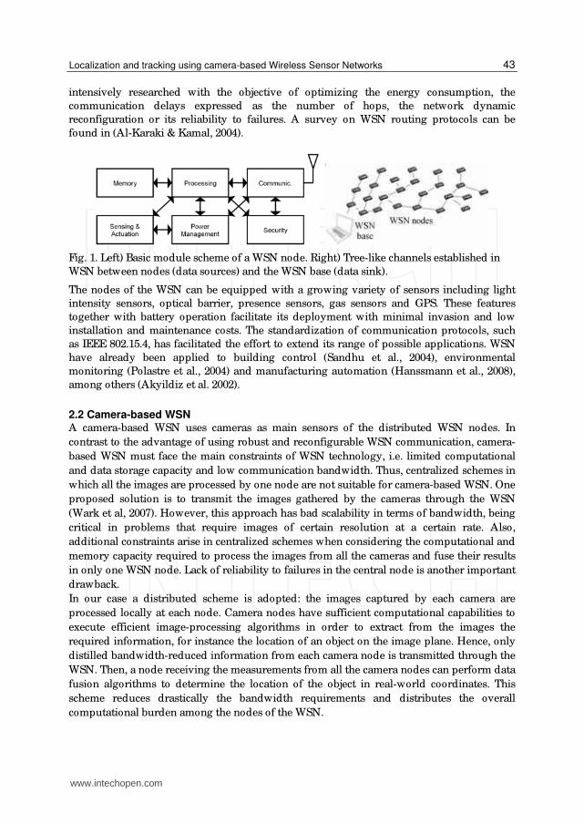
2.1 Brief introduction to wireless sensor networks A Wireless Sensor Network (WSN) consists of a large number of spatially distributed

devices (nodes) with sensing, data storage, computing and wireless communication

capabilities. Low size, low cost and particularly low power consumption are three of the key

issues of WSN technology. Nodes are designed to operate with minimal hardware and

software requirements, see basic scheme of the main modules in Fig. 1Left. They often use 8

or 16-bit microcontrollers at low processing rates and a limited RAM capacity for data

storage. Nodes often require a few milliwatts for operation. Most nodes can be set in a

standby state, from which they wake up occasionally, for instance when one sensor detects

an event. Their radio transceivers are also very energy efficient and their transmission range

is typically less than 100 m in the open air. Besides, its bandwidth is often low.

In contrast to the simplicity of each node, the main strengths of WSN rely on the cooperation

of a number of nodes for cooperatively performing tasks. In fact, a good number of

algorithms have been developed to provide them significant flexibility, scalability, tolerance

to failures and self-reconfiguration. WSN are typically organized in tree-like channels

between data sources (nodes) and data sinks (WSN base), see Fig. 1Right. Despite this

apparent simplicity, algorithms for network formation and information routing have been

www.intechopen.com

Localization and tracking using camera-based Wireless Sensor Networks

43

intensively researched with the objective of optimizing the energy consumption, the

communication delays expressed as the number of hops, the network dynamic

reconfiguration or its reliability to failures. A survey on WSN routing protocols can be

found in (Al-Karaki & Kamal, 2004).

Fig. 1. Left) Basic module scheme of a WSN node. Right) Tree-like channels established in

WSN between nodes (data sources) and the WSN base (data sink).

The nodes of the WSN can be equipped with a growing variety of sensors including light

intensity sensors, optical barrier, presence sensors, gas sensors and GPS. These features

together with battery operation facilitate its deployment with minimal invasion and low

installation and maintenance costs. The standardization of communication protocols, such

as IEEE 802.15.4, has facilitated the effort to extend its range of possible applications. WSN

have already been applied to building control (Sandhu et al., 2004), environmental

monitoring (Polastre et al., 2004) and manufacturing automation (Hanssmann et al., 2008),

among others (Akyildiz et al. 2002).

2.2 Camera-based WSN A camera-based WSN uses cameras as main sensors of the distributed WSN nodes. In

contrast to the advantage of using robust and reconfigurable WSN communication, camera-

based WSN must face the main constraints of WSN technology, i.e. limited computational

and data storage capacity and low communication bandwidth. Thus, centralized schemes in

which all the images are processed by one node are not suitable for camera-based WSN. One

proposed solution is to transmit the images gathered by the cameras through the WSN

(Wark et al, 2007). However, this approach has bad scalability in terms of bandwidth, being

critical in problems that require images of certain resolution at a certain rate. Also,

additional constraints arise in centralized schemes when considering the computational and

memory capacity required to process the images from all the cameras and fuse their results

in only one WSN node. Lack of reliability to failures in the central node is another important

drawback.

In our case a distributed scheme is adopted: the images captured by each camera are

processed locally at each node. Camera nodes have sufficient computational capabilities to

execute efficient image-processing algorithms in order to extract from the images the

required information, for instance the location of an object on the image plane. Hence, only

distilled bandwidth-reduced information from each camera node is transmitted through the

WSN. Then, a node receiving the measurements from all the camera nodes can perform data

fusion algorithms to determine the location of the object in real-world coordinates. This

scheme reduces drastically the bandwidth requirements and distributes the overall

computational burden among the nodes of the WSN.

www.intechopen.com


44

In the adopted scheme, each camera node applies image-processing segmentation

techniques to identify and locate the object of interest on the image plane. Thus, the

possibility of flexibly programming image processing algorithms is a strong requirement.

The selected camera board is the CMUcam3, an open source programmable board endowed

with a color detector with 352x288 pixels. Figure 2 shows a picture of a camera node

comprised of an Xbow node and one CMUcam3 board.

Fig. 2. CMUcam3 integrated with a Xbow node.

We implemented a robust algorithm based on a combination of color and motion

segmentations capable of being efficiently executed with limited computational and

memory resources. The result of the segmentation algorithm is a rectangular region on the

image plane characterized by the coordinates of its central pixel, its width and height.

Several data fusion methods are used to merge the results from the segmentation algorithms

running in every camera node. Data fusion reduces the influence of errors in measurements

and increases the overall system accuracy. On the other hand, it requires having the

measurements from all the cameras expressed in the same reference frame. In the methods

presented, each camera node obtains the coordinates of the region of interest on the image

plane applying image segmentation algorithms and corrects its own optical distortions

transforming them to the undistorted normalized pin-hole projection on the image plane.

Each camera is internally calibrated and the calibration parameters are known at each

camera node. Hence, camera nodes message packets include the distortion-corrected

normalized measurements for each image analyzed. These messages are transmitted

through the WSN for data fusion. This approach standardizes the measurements from all

camera nodes facilitating data fusion method and distributes the computational cost among

the camera nodes. For further details of the implementations refer to Section 6.

3. Localization using maximum likelihood

Maximum Likelihood (ML) is one of the basic statistical data fusion methods, (Mohammad-

Djafari, 1997). Its objective is to estimate the state of an event that best justifies the

observations maximizing a statistical likelihood function that can be expressed as the

probability of measurement z conditioned to state x:

www.intechopen.com


45

{ }ˆ arg max ( | )x

x P z x= (1)

Assume that the state is measured synchronously from N different sensors z1,...,zN, where zi

is the measurement gathered by sensor i. Supposed the measurements of all the sensor

z1,...,zN can be considered statistically independent, the overall likelihood function can be

expressed by:

11

( ,..., | ) ( | )N

N ii

p z z x p z x=

= ∏ (2)

Assume that each measurement is subject to errors that can be considered to be originated

by the influence of a high number of independent effects. By virtue of the Central Limit

Theorem it can be considered to have Gaussian distribution, (Rice, 2006):

( ) ( )-1- -

2 -11( | ) det(2 ) exp

2

Ti i i i ip z x Σ z x Σ z xπ

− = (3)

where Σi is the covariance of measurements from sensor i. The ML method estimates the

state as the following weighted sum:

( ) ( )-1

1 1 1 11 1 1- - - -

N N Nx Σ + + Σ Σ z + + Σ z= (4)

where each measurement is weighted proportionally to the inverse of its covariance:

measurements with more noise have lower weigh in (4). The overall estimated covariance

follows the expression:

( )1

1 11

-- -

x NΣ = Σ + + Σ (5)

It should be noted that since Σx <Σi the estimate is more accurate than any measure.

The following describes the ML method adopted for camera-based WSN. Consider that a

point P in the environment is observed by N camera nodes. pi=[xi yi] are the distortion-

corrected pixel coordinates of P viewed from camera node i. Before applying (4) it is

necessary to have the measurements from all the cameras in the same reference frame.

Let frame Fi be a reference frame local to camera i. The location and orientation of the N

cameras in a global reference frame G are known. Let Ti be the transformation matrix from

frame Fi to frame G. Assume that Zi, the Z coordinate of P in frame Fi, is known. Taking into

account the pin-hole model it is possible to project pixel pi at distance Zi:

[ ] [ ]=T T

i i i i i i i i iP X Y Z = x Z y Z Z (6)

Pi represents the coordinates of P measured by camera i and expressed in frame Fi. Using Ti

Pi can be transformed to frame G applying:

-1

11

Gii

i

PPT

= (7)

www.intechopen.com


46

PiG represents the coordinates of P in frame G as measured by camera i. With the

measurements from all the cameras in the same frame G, the ML method can be applied.

Assume that PiG contains Gaussian errors with covariance matrix Σi. Supposed the

measurements from different cameras statistically independent, the ML method estimates P

with measurements PiG using (4).

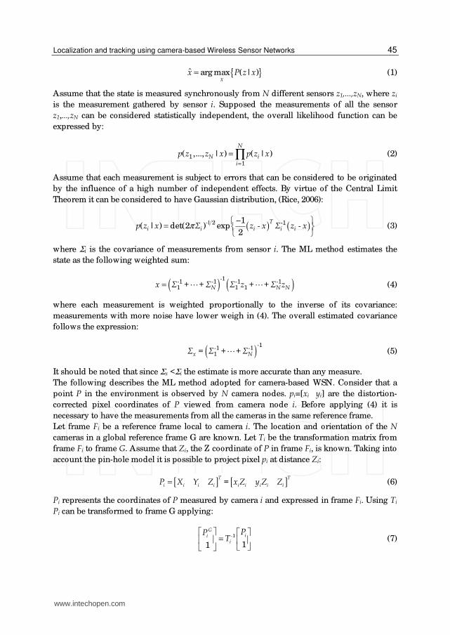
Σi can be decomposed in an eigenvector matrix and an eigenvalue matrix, Σi=LΛL-1. The

eigenvectors of Σi form the columns of L. The eigenvectors are orthonormal vectors that

represent the axes of frame Fi in the global frame G. Λ is a diagonal matrix. The elements of

the diagonal are the eigenvalues of Σi, which are the variance associated to PiG at each axis of

frame Fi. L and Λ, and thus Σi can be easily constructed knowing the orientation of camera i and estimating the noise in the measurements.

Figure 3 shows an illustration of the method with two cameras. The probability distribution

of the measurements from Camera1 and Camera2 are represented in cyan color. The

probability distribution of the fused estimate is in blue. The remarkable reduction in the

covariance denotes an increment in the fused estimate.

Fig. 3. Example illustrating ML data fusion method.

The described ML method can be executed in a WSN node in few milliseconds. This high

efficiency facilitates schemes where camera nodes observing the same object interchange

their observations and apply data fusion.

This method can be used for object localization but it is not suitable for object tracking, and

even when used for localization the ML method has important constraints. Applying the ML

data fusion requires having previously determined Zi, the location of P in frame Fi. A typical

approach is to set Zi with an average value and compensate the error assuming a high value

for the variance of the error at the Z axis of Fi. However, this artificial increase of uncertainty

decreases the quality of the overall estimate. Another approach is to use, under an iterative

scheme, the value of Zi at time t-1. Nevertheless, this method requires assuming an initial

value and, errors in estimation at time t-1 involve errors at subsequent iterations.

Furthermore, ML has high sensitivity to failures in measurements, for instance in cases

where the object is out of the field of view of the camera, occluded in the image or in case of

losses of WSN messages, not infrequent in some environments. This sensor fusion method

relies totally on the measurements and its performance degrades when some of them are

lost. Other sensor fusion techniques such as Bayesian Filters rely on observations and on

models, which are very useful in case of lack of measurements.

www.intechopen.com


47

4. Localization and tracking using EIF

Bayesian Filters (RBFs) provide a well-founded mathematical framework for data fusion.

RBFs estimate the state of the system assuming that measurements and models are subject

to uncertainty. They obtain an updated estimation of the system state as a weighted average

using the prediction of its next state according to a system model and also using a new

measurement from the sensor to update the prediction. The purpose of the weights is to give

more trust to values with better (i.e., smaller) estimated uncertainty. The result is a new state

estimate that lies in between the predicted and measured state, and has a better estimated

uncertainty than either alone. This process is repeated every step, with the new estimate and

measure of uncertainty used as inputs for the following iteration.

The Kalman Filter (KF) is maybe the most commonly used RBF method. The Kalman Filter

and its dual, the Information Filter (IF), use a prediction model, that reflects the expected

evolution of the state, and a measurement model, that takes into account the process

through which the state is observed to respectively predict and update the system state:

( )

( )

= +ε

= + δ

-1t t t

t t t

x g x

z h x (8)

xt is the current system state vector, xt-1 is the previous state vector, zt is the measurement

vector and ┝t and ├t are White Gaussian Noise (WGN) parameterized by their mean value

and a covariance matrix.

In our problem the measurements considered are the location of the object on the image of

the distributed camera nodes. Even assuming simple pin-hole cameras, these observation

models are non-linear and a first order linearization is required. In this case, having non-

linear prediction and measurement models leads to the Extended Information Filter (EIF).

After linearizing the IF equations via Taylor Expansion, we can assume that the predicted

state probability, written as Gaussian, is as follows:

( ) ( )

( ) ( )( ) ( ) ( )( )

1 2

1

11 1 1 1 1 1

det 2

1 exp

2

-t t t

T

t t- t t - t - t t t- t t - t -

p x |x πR

- x - g μ - G x - μ R x - g μ - G x - μ

−

−

=

(9)

where 1t−µ is the mean of the previous state, Rt is the covariance of the prediction model

(correspondent to ┝t ) and Gt is the Jacobian matrix of g. The next state probability, written as

Gaussian, is as follows:

( ) ( )

( ) ( )( ) ( ) ( )( )-

1 2

1

det 2

1 exp

2

-t t t

T

t t t t t t t t t t t

p z |x πQ

- z - h μ - H x - μ Q z - h μ - H x - μ

=

(10)

where tµ is the mean of the predicted state, Qt is the covariance of the measurement model

(correspondent to ├t) and Ht is the Jacobian matrix of h.

Information Filters (IF) employ the so-called canonical representation, which consists of an

information vector ξ=Σ-1μ and matrix Ω=Σ-1. Figure 4 shows the full EIF algorithm. In each

recursive iteration it computes the current system state (ξt , Ωt) from the previous state and

www.intechopen.com


48

the new measurement (ξt-1, Ωt-1, zt). Each iteration is divided in two steps: prediction (lines 1-

4 in Fig. 4) and update (lines 5, 6). For more details, refer to (Thrun et al., 2005).

Since both g and h require the state as an input, it is mandatory to recover the state estimate

μ from canonical parameters (see step 1 of the EIF algorithm in Fig. 4) which makes the

prediction stage from the algorithm lose efficiency compared to the EKF. Nevertheless, the

update stage of EIF is much more efficient than EKF and thus the former is more suitable

when there are a large number of observations. In this sense, the efficiency of this algorithm

with respect to other implementations is improved when a simple prediction model

together with a large measurement vector zt are used. Besides, Information Filters are also

numerically more stable and are more suitable for characterizing and representing

information and its absence, Ω=0.

Extended_Information_Filter (ξt-1 , Ωt-1 , zt ):

1: -1-1 -1 -1t t tµ ξ= Ω

2: ( )-1

-1-1

Tt t t t tG G RΩ = Ω +

3: ( )-1t tt gξ µ= Ω

4: ( )-1t tgµ µ=

5: -1Ttt t t tH Q HΩ = Ω +

6: ( )--

1Tt t t t t t t tH Q z h Hξ ξ µ µ = + +

7: return ξt , Ωt

Fig. 4. EIF algorithm.

Therefore, the selection of the state and models has critical impact on the performance and

computational burden of the filter. We selected a state vector typical in tracking problems

that considers only the current object position and velocity xt=[Xt Yt Zt Vxt Vyt Vzt]T. In our

problem we can have a large number of inexpensive camera nodes. We preferred EIF over

EKF due to its better scalability with the number of observations. Also, we assumed a very

simple local linear motion model to reduce the burden of the prediction stage in EIF:

− − −

− − −

− − −

= + = = + = = + =

1 1 1

1 1 1

1 1 1

t t t t t

t t t t t

t t t t t

X X Vx Vx Vx

Y Y Vy Vy Vy

Z Z Vz Vz Vz

(11)

Of course, we do not know a priori what kind of movement would the object perform. So

we assume local linear motion and we include Gaussian noise in each coordinate to consider

errors in the model. This model can efficiently represent local motions and has been

extensively applied in RBFs. Also, more complex models increase the computation burden

and would require a priori knowledge of the motion, unavailable in tracking of objects with

no collaboration, as is the case of security applications.

The EIF uses a different observation model for each camera that is seeing the object. The

observation model adopted for camera i uses as measurements the distortion-corrected pin-

hole projections from camera i at time t, pi,t. To allow the estimation of the object velocity, we

www.intechopen.com


49

also include in the measurement the projection from camera i at time t-1, pi,t-1. The

measurement vector including measurements from all the N cameras that are tracking the

object can be written as zt=[p1,t p1,t-1 p2,t p2,t-1 … pN,t pN,t-1]T.

The location of the object at time t in the global reference frame G, Pt, can be computed from

pi,t, its projection in the image plane of camera node i, as described in (6) and (7). Provided Ti

is the transformation matrix of Fi, the reference frame of camera i, and ti,j represents the j-th

row of Ti, the measurement from each camera node i can be related to the target position as:

[ ] [ ]

[ ] [ ]1 3,

,

,2 3

1 1

1 1

T T

i, t i, ti t

i t T Ti t

i, t i, t

t P t Pxp = =

y t P t P

(12)

Thus, the overall measurement model h which relates zt with xt can be written as:

[ ] [ ]

[ ] [ ],1 ,3

1, 1, 1 , , 1 ,

,2 ,3

1 1,

1 1

T T

i t t t i t t tTt t N t N t i t T T

i t t t i t t t

t X Y Z t X Y Zh h h h h h

t X Y Z t X Y Z− −

= = (13)

This observation model is, as already stated, non-linear. At the updating stage the EIF

requires using the Jacobian matrices of h, Ht.

Each measurement at each camera node i requires only one prediction step and one

updating step. Assuming 3 cameras, the execution of an iteration of an EIF for 2D

localization and tracking with 3 cameras requires approximately 6,000 floating point

operations, roughly 400 ms. in a Xbow TelosB mote, such as those used in the experiments.

The Bayesian approach provides high robustness in case of losses of measurements. If at

time t there are no measurements, only the prediction stage of the EIF algorithm is executed.

In this case, the uncertainty of the state grows more and more until new measurements are

available. This behavior naturally increases the robustness in case of failures of the

segmentation algorithm or losses of measurement messages. Thus, EIF exhibits higher

robustness than ML to noisy measurements and particularly to the lack of measurements.

Some experimental results can be found in Section 7.

5. Active perception techniques

In the previous schemes all the cameras that are seeing the object at any time t are used for

data fusion regardless of the usefulness of the measurement they provide for the overall

estimation. In this section we briefly summarize an entropy-based active perception

approach that dynamically activates or deactivates each camera node balancing the

information it effectively provides and the cost of the measurement.

The active perception problem can be broadly defined as the procedure to determine the

best actions that should be performed. In our problem there are two types of actions,

activate or deactivate camera i. Given a certain system state x, each action a involves an

impact on the perception, i.e. it obtains a certain reward r(x,a). Also, each action has a certain

cost c(x,a). For instance, by activating camera node i, the reward is a perception with lower

uncertainty, and the cost is the increase of energy consumption.

In most active perception strategies the selection of the actions is carried out using reward

VS cost analyses. In the so-called greedy algorithms the objective is to decide the next best

action to be carried out without taking into account long-term goals. POMDPs (Kaelbling et

www.intechopen.com


50

al., 1998), on the other hand, consider the long-term goals providing an elegant way to

model the interaction of an agent in an environment, both of them uncertain. Nonetheless,

POMDPs require intense computing resources and memory capacity. POMDPs also scale

badly with the number of camera nodes. Thus, in our problem we adopted an efficient

greedy active perception scheme.

At each time step, the strategy adopted activates or deactivates one camera node taking into

account the expected information gain and the cost of the measurement. In our approach the

reward is the information gain about the target location due to the new observation.

Shannon entropy is used to quantify the information gain.

Consider the prior target location distribution at time t to be p(xt). If camera node i, currently

unused, is activated and its measurement is available at t, then the posterior target location

distribution will be p(xt|zi). Then, the gain of information from activating camera node i can

be expressed by H(xt)-H(xt|zi), where H(xt) and H(xt|zi) stand for the Shannon entropy of

p(xt) and p(xt|zi). H(xt)-H(xt|zi) also denotes the mutual information between xt and zi.

Entropy is a measure of the uncertainty associated to a random variable, i.e. the information

content missing when one does not know the value of a random variable. The reward for

action a=A(i) -activating camera node i- is expressed by:

( ) ( ), ( ) ( )t t t ir x a A i H x H x z= = − (14)

There are analytical expressions to express the entropy of a Gaussian distribution. Assuming

p(xt) and p(xt|zi) are Gaussians the reward of an action can be computed with:

( ) 1

2

1, ( ) log

2tr x a A i

= =

Σ

Σ (15)

where Σ1 and Σ2 are the covariance matrices of distributions p(xt) and and p(xt|zi).

On the other hand, the cost of activating a camera node is mainly expressed in terms of the

energy consumed by camera. However, note that there are other costs, as those associated to

the use of the wireless medium for transmitting the new measurements or the increase in

computational burden required to consider the measurements from the new camera in the

EIF. Also, these costs can vary depending on the camera node and the currently available

resources. For instance, the cost of activating a camera with low battery level is higher than

activating one with full batteries.

An action aj is defined as advantageous at certain time t if the reward is higher than the cost,

i.e. r(xt,aj)>c(xt,aj). In a system with a set of potential advantageous actions, a∈A+, the more

advantageous action is selected to be carried out:

( ) ( )( )ˆ arg max , ,j

t j t ja A

a r x a c x a+∈

= − (16)

This active perception method can be easily incorporated within a Bayesian Recursive Filter.

In our case it was integrated in the EIF described in Section 5. To simplify the complexity

and computer burden, the number of actions that can be done at each time is limited to one.

Thus, in a deployment with N cameras the number of actions analyzed at each time is N:

deactivation of each of the currently active camera nodes and activation of each of the

currently unused camera nodes. The most advantageous action is selected to be carried out.

www.intechopen.com


51

The main disadvantage of (14) is that the action to be carried out should be decided without

actually having the new measurement. We have to rely on estimations of future information

gain. At time t the information matrix of the EIF at t is Ωt. In the prediction stage the

information matrix is predicted, 1t+Ω , see the EIF algorithm in Fig. 4. In the update stage, it

is updated, Ωt+1, using the observation models of the sensors currently used. In case of

performing sensory action a, the observation model would change and involve a new

updated information matrix Ωat+1. The expectation of the information gain can be

approximated by ½·log(|Ωat+1|/ |Ωt+1|).

This expression assumes that the location distribution of the target is Gaussian, which is not

totally exact due to the nonlinearities in the observation pin-hole models. Also, they provide

expectation of the information gain instead of the information gain itself. Despite these

inaccuracies, it is capable of providing a useful measure of the information gain from a

sensory action in an efficient way. In fact, the active perception method for a setting with 3

cameras adopted requires approximately 3,400 floating point operations, roughly 300 ms in

Xbow TelosB motes, but can imply remarkable resources saving rates, up to 70% in some

experiments shown in Section 6. It should be noted that its computational burden scales well

since it is proportional to the number of cameras in the setting.

6. Implementation and some results

This Section provides details of the camera-based WSN implementation and presents some

experimental results.

6.1 Implementation of camera-based WSN with COTS equipment Requirements such as energy consumption, size and weight are very important in these

systems. In our experiments we used TelosB motes from Xbow Inc (http:/ / www.xbow.com).

These motes use a Texas Instruments MPS430 16-bit microprocessor at 8 MHz, which can be

enough to execute algorithms with low computer-burden but is not capable of applying

image processing methods with sufficient image resolution and frame rate. The RAM

memory of TelosB (10 KB) is also insufficient for most image processing techniques. In

previous developments we also used Xbow Mica2 motes, with lower resources.

The micro camera board selected is the CMUcam3 (http:/ / www.cmucam.org). It is an open

source programmable embedded platform connected to an Omnivision 1/ 4’’ CMOS 352x288

color detector. Its main processor, the NXP LPC2106, allows implementing, in Custom C,

code-efficient real-time image processing algorithms. Different lenses (of up to 150º FOVH)

were used in the experiments to accommodate the dimensions of the environment. Figure 5

shows a set of camera nodes. They were mounted on small tripods to facilitate deployment

and orientation. In preliminary works we used CMUcam2 boards. The main practical

advantages of CMUcam3 over CMUcam2 are the possibility of being programmed

(CMUcam2 used fixed pre-programmed algorithms instead) and a high reduction in energy

consumption.

Each CMUcam3 is connected to a single Xbow mote though a RS-232 link. The CMUcam3

board captures the images and executes the algorithms for object segmentation while the

Xbow mote runs a series of algorithms required for cooperative location and tracking

including control of the CMUcam3, correction of optical distortions, algorithms for

synchronization among the camera nodes and wireless transmission of the measurements.

From the Xbow side, CMUcam3 operates transparently as any other sensor.

www.intechopen.com


52

Fig. 5. Set of camera nodes equipped with CMUcam2 and CMUcam3 micro cameras.

6.1.1 Image segmentation Although CMUcam3 offers programming facilities, its limited computational and memory

resources require efficient algorithm design and coding to achieve near to real-time

processing capabilities. In fact, the constraints in their memory capacity prevent from

loading the whole image in the RAM memory and block-based processing is required.

We assume that the objects of interest are mobile. First, assuming a static environment, the

moving objects are identified through difference with respect to a reference image. A pixel

of image k Imk(x,y) is considered part of a mobile object if |Imk(x,y)-Imref(x,y)|>T, where T is

a color threshold and Imref(x,y) is the reference image. To reduce computer burden, images

are divided in windows and if the number of pixels which color has changed is above NP,

the window is considered with motion.

In case the color of the object of interest can be characterized, then a color-based

segmentation is applied only to the windows with motion previously identified. For this

operation the HSI color field is preferred in order to achieve higher stability of color with

lighting changes. Then, an efficient 8-neighbours region-growing algorithm is used. Finally,

the characteristics of the region of interest such as coordinates of the central pixel, region

width and height are obtained. Figure 6 shows the results of each step over an image from a

CMUcam3 in which a fireman is segmented.

Fig. 6. Left) Object segmentation using motion.Right) Object segmentation using color.

The algorithm has been efficiently programmed so that the complete segmentation (the

images are 352x288 pixels) takes 560 ms., 380 ms. of which are devoted to downloading the

image from the internal camera buffer to the CMUcam3 board memory.

6.1.2 Image distortions correction In the next step, before transmitting the measurements for data fusion, each camera node

corrects its own optical distortions, transforming them to the normalized pin-hole

www.intechopen.com


53

projection. Let Pi=[Xi Yi Zi]T be the coordinates of a point in the environment expressed in

reference frame local to camera i, Fi. Assuming an ideal pin-hole model, the normalized

projection of Pi on the image plane of camera i is pi=[X/Z Y/Z]T=[xi yi]T. After including lens

radial and tangential distortions, the distorted point pid=[xid yid]T is defined as follows:

d r ti i i ip d p d= + (17)

where dir and dit are simplified radial and tangential distortions terms as defined in the

model described in (Heikkilä & Silven, 1997):

( )

2 2

2 4

2 2

2 ( 2 )1

2 2

i i i ir ti i i i

i i i i

cx y d r xd ar br d

c r y dx y

+ += + + =

+ + (18)

where ri2=xi2+yi2. Finally, assuming the skew factor is zero, the pixel coordinates on the

image pip=[xip yip]T are determined considering the focal length f and the coordinates of the

principal point of the lens cc of camera i by using the following expression:

p di ip fp cc= + (19)

The internal calibration parameters -optical distortion parameters a, b, c and d, the focal

distance f and the coordinates of the principal point of the lens cc- are considered known at

each camera node. Consider pip is the pixel coordinates of the centre of a region of interest

segmented in the images. The correction is applied in two steps: obtain pid using (19) and

compute pi using (17) and (18). For practical purposes (18) is usually approximated using xid

and yid instead of xi and yi. Thus, pi=[xi yi]T can be computed efficiently involving only two

divisions and few products and sums. It is executed in the Xbow node itself.

Also, the position and orientation for each camera in a global reference frame are assumed

known at each camera node. These 6 parameters -3 for camera position and 3 for

orientation- are included in the measurements packets sent for data fusion so that it can

cope with static and mobile cameras, for instance on very light-weight UAVs. The time

stamps of the measurements are also included in these packets for synchronization.

6.1.3 Interface and synchronization modules Several software modules were implemented on the Xbow mote. One of them implements

the command interface with the CMUcam3 using low-level TinyOS routines. The node

commands the CMUcam3 to start capturing images at a certain rate and to execute object

segmentation to the captured images. For each image, the CMUcam3 replies the

characteristics of the region segmented (centre, width and height). Then, the distortion

correction method described in Section 6.1.2 is applied. Finally, the resulting measurements

are sent through the WSN for data fusion. It should be noted that the Xbow nodes can

disable or enable the operation of the CMUcam3 board, allowing active perception

techniques such as those described in Section 5.

Another software module was devoted to synchronization among camera nodes. The

method selected is the so-called Flooding Time Synchronization Protocol (FTSP) (Maróti et al.,

2004). This algorithm establishes hierarchies among the WSN nodes. The leader node

periodically sends a synchronization message. Each camera node that receives the message

resends it following a broadcast strategy. The local time of each camera node is corrected

www.intechopen.com


54

depending on the time stamp on the message and the sender of the message. The resulting

synchronization error is of few milliseconds.

6.2 Some results Figure 7Left shows a picture of one localization and tracking experiment. The objective is to

locate and track mobile robots that follow a known trajectory, taken as ground truth. Figure

7Right depicts a scheme of an environment involving 5 camera nodes at distributed

locations and with different orientations. The local reference frames of each of the camera

are depicted. The global reference frame is represented in black.

In this Section the three data fusion methods presented are compared in terms of accuracy

and energy consumption. Accuracy is measured as the mean error with the ground truth.

For the consumption analysis we will assume that the energy dedicated by the Xbow node to

execute any of the three data fusion algorithms is significantly lower than the energy

devoted by a camera node to obtain observations. The latter includes the energy required for

image acquisition and segmentation in the CMUcam3 boards. The energy consumed by a

camera node during an experiment is proportional to the number of measurements made.

In all the experiments the commands given to the robot to generate the motion were the

same. The object locations are represented with dots in Fig. 7Right. In all the experiments

the measurements computed by cameras 2 and 3 from t=10 s. to t=25 s. are considered lost

and cannot be used for data fusion. The object locations within this interval are marked with

a rectangle in Fig. 7Right.

Fig. 7. Left) Object tracking experiment using 3 CMUcam3 micro cameras. Right) Scheme of

the environment involving 5 camera nodes.

Four different cases were analyzed: ML using cameras 1, 2 and 3; EIF using cameras 1, 2 and

3; EIF using the five cameras; and active perception with all the cameras. A set of ten

repetitions of each experiment were carried out. Figures 8a-d shows the results obtained for

axis X (left) and Y (right) in the four experiments. The ground truth is represented in black

color and the estimated object locations are in red. In Figs. 8b-d the estimated 3σ confidence

interval is represented in blue color. Table 1 shows the average of the mean error and the

number of measurements used by each method.

www.intechopen.com


55

a)

b)

c)

d)

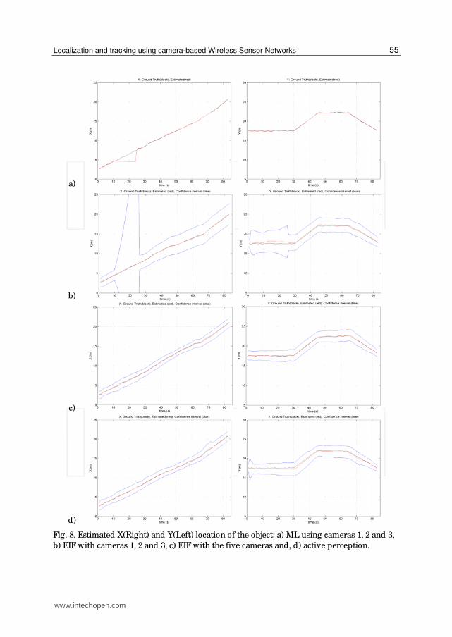
Fig. 8. Estimated X(Right) and Y(Left) location of the object: a) ML using cameras 1, 2 and 3,

b) EIF with cameras 1, 2 and 3, c) EIF with the five cameras and, d) active perception.

www.intechopen.com


56

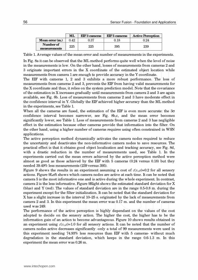
ML EIF 3 cameras EIF 5 cameras Active Perception

Mean error (m.) 0.42 0.37 0.18 0.24

Number of

measurements 225 225 395 239

Table 1. Average values of the mean error and number of measurements in the experiments.

In Fig. 8a it can be observed that the ML method performs quite well when the level of noise

in the measurements is low. On the other hand, losses of measurements from cameras 2 and

3 originate important errors in the X coordinate of the estimated object location while

measurements from camera 1 are enough to provide accuracy in the Y coordinate.

The EIF with cameras 1, 2 and 3 exhibits a more robust performance. The loss of

measurements from cameras 2 and 3, prevents the EIF from having valid measurements for

the X coordinate and thus, it relies on the system prediction model. Note that the covariance

of the estimation in X increases gradually until measurements from camera 2 and 3 are again

available, see Fig. 8b. Loss of measurements from cameras 2 and 3 have moderate effect in

the confidence interval in Y. Globally the EIF achieved higher accuracy than the ML method

in the experiments, see Table 1.

When all the cameras are fused, the estimation of the EIF is even more accurate: the 3σ

confidence interval becomes narrower, see Fig. 8b,c, and the mean error becomes

significantly lower, see Table 1. Loss of measurements from cameras 2 and 3 has negligible

effect in the estimation because other cameras provide that information into the filter. On

the other hand, using a higher number of cameras requires using often constrained in WSN

applications.

The active perception method dynamically activates the camera nodes required to reduce

the uncertainty and deactivates the non-informative camera nodes to save resources. The

practical effect is that it obtains good object localization and tracking accuracy, see Fig. 8d,

with a drastic reduction in the number of measurements used, see Table 1. In the

experiments carried out the mean errors achieved by the active perception method were

almost as good as those achieved by the EIF with 5 cameras (0.24 versus 0.18) but they

needed 39.49% less measurements (239 versus 395).

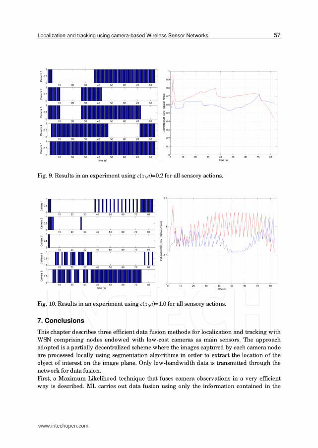
Figure 9 shows the results in an experiment assuming a cost of c(xt,a)=0.2 for all sensory

actions. Figure 9Left shows which camera nodes are active at each time. It can be noted that

camera 5 is the most informative one and is active during the whole experiment. In contrast,

camera 2 is the less informative. Figure 9Right shows the estimated standard deviation for X

(blue) and Y (red). The values of standard deviation are in the range 0.5-0.8 m. during the

experiment except for the filter initialization. It can be noted that the standard deviation for

X has a slight increase in the interval 10–25 s. originated by the lack of measurements from

camera 2 and 3. In this experiment the mean error was 0.17 m. and the number of cameras

used was 249.

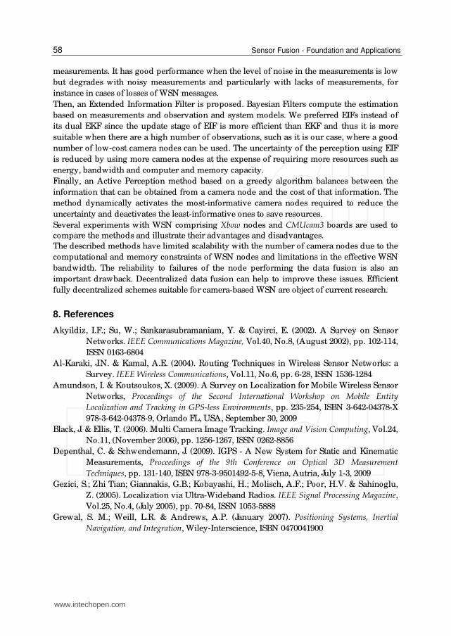
The performance of the active perception is highly dependant on the values of the cost

adopted to decide on the sensory action. The higher the cost, the higher has to be the

information gain of an action to become advantageous. Figure 10 shows results obtained in

an experiment using c(xt,a)=1.0 for all sensory actions. It can be noted that the number of

camera nodes active decreases significantly -only a total of 99 measurements were used in

this experiment needing 74.93% less resources than EIF with 5 cameras- without much

degradation in the standard deviation, which keeps in the range 0.6-1.3 m. In this

experiment the mean error was 0.26 m.

www.intechopen.com


57

Fig. 9. Results in an experiment using c(xt,a)=0.2 for all sensory actions.

Fig. 10. Results in an experiment using c(xt,a)=1.0 for all sensory actions.

7. Conclusions

This chapter describes three efficient data fusion methods for localization and tracking with

WSN comprising nodes endowed with low-cost cameras as main sensors. The approach

adopted is a partially decentralized scheme where the images captured by each camera node

are processed locally using segmentation algorithms in order to extract the location of the

object of interest on the image plane. Only low-bandwidth data is transmitted through the

network for data fusion.

First, a Maximum Likelihood technique that fuses camera observations in a very efficient

way is described. ML carries out data fusion using only the information contained in the

www.intechopen.com


58

measurements. It has good performance when the level of noise in the measurements is low

but degrades with noisy measurements and particularly with lacks of measurements, for

instance in cases of losses of WSN messages.

Then, an Extended Information Filter is proposed. Bayesian Filters compute the estimation

based on measurements and observation and system models. We preferred EIFs instead of

its dual EKF since the update stage of EIF is more efficient than EKF and thus it is more

suitable when there are a high number of observations, such as it is our case, where a good

number of low-cost camera nodes can be used. The uncertainty of the perception using EIF

is reduced by using more camera nodes at the expense of requiring more resources such as

energy, bandwidth and computer and memory capacity.

Finally, an Active Perception method based on a greedy algorithm balances between the

information that can be obtained from a camera node and the cost of that information. The

method dynamically activates the most-informative camera nodes required to reduce the

uncertainty and deactivates the least-informative ones to save resources.

Several experiments with WSN comprising Xbow nodes and CMUcam3 boards are used to

compare the methods and illustrate their advantages and disadvantages.

The described methods have limited scalability with the number of camera nodes due to the

computational and memory constraints of WSN nodes and limitations in the effective WSN

bandwidth. The reliability to failures of the node performing the data fusion is also an

important drawback. Decentralized data fusion can help to improve these issues. Efficient

fully decentralized schemes suitable for camera-based WSN are object of current research.

8. References

Akyildiz, I.F.; Su, W.; Sankarasubramaniam, Y. & Cayirci, E. (2002). A Survey on Sensor

Networks. IEEE Communications Magazine, Vol.40, No.8, (August 2002), pp. 102-114,

ISSN 0163-6804

Al-Karaki, J.N. & Kamal, A.E. (2004). Routing Techniques in Wireless Sensor Networks: a

Survey. IEEE Wireless Communications, Vol.11, No.6, pp. 6-28, ISSN 1536-1284

Amundson, I. & Koutsoukos, X. (2009). A Survey on Localization for Mobile Wireless Sensor

Networks, Proceedings of the Second International Workshop on Mobile Entity

Localization and Tracking in GPS-less Environments, pp. 235-254, ISBN 3-642-04378-X

978-3-642-04378-9, Orlando FL, USA, September 30, 2009

Black, J. & Ellis, T. (2006). Multi Camera Image Tracking. Image and Vision Computing, Vol.24,

No.11, (November 2006), pp. 1256-1267, ISSN 0262-8856

Depenthal, C. & Schwendemann, J. (2009). IGPS - A New System for Static and Kinematic

Measurements, Proceedings of the 9th Conference on Optical 3D Measurement

Techniques, pp. 131-140, ISBN 978-3-9501492-5-8, Viena, Autria, July 1-3, 2009

Gezici, S.; Zhi Tian; Giannakis, G.B.; Kobayashi, H.; Molisch, A.F.; Poor, H.V. & Sahinoglu,

Z. (2005). Localization via Ultra-Wideband Radios. IEEE Signal Processing Magazine,

Vol.25, No.4, (July 2005), pp. 70-84, ISSN 1053-5888

Grewal, S. M.; Weill, L.R. & Andrews, A.P. (January 2007). Positioning Systems, Inertial

Navigation, and Integration, Wiley-Interscience, ISBN 0470041900

www.intechopen.com


59

Grocholsky, B.; Keller, J.; Kumar, V. & Pappas, G. (2006). Cooperative Air and Ground

Surveillance, IEEE Robotics & Automation Magazine, Vol.13, No.3, pp. 16-25, ISSN

1070-9932

Hanssmann, M.; Rhee, S. & Liu, S. (2008). The Applicability of Wireless Technologies for

Industrial Manufacturing Applications Including Cement Manufacturing,

Proceedings of the IEEE Cement Industry Technical Conference 2008, pp.155-160, ISBN

978-1-4244-2080-3, Miami FL, USA, May 18-22, 2008

Heikkila, J. & Silven, O. (1997). A Four-step Camera Calibration Procedure with

Implicit Image Correction, Proceedings of the 1997 Conference on Computer Vision and

Pattern Recognition, pp. 1106, ISBN 0-8186-7822-4, San Juan, Puerto Rico, June 17-19,

1997.

Kaelbling, L.P.; Littman, M.L. & Cassandra A.R. (1998). Planning and acting in partially

observable stochastic domains. Artificial Intelligence, Vol.101, No.1-2, pp. 99–134,

ISSN 0004-3702

Maróti, M.; Kusy, B.; Simon G. & Lédeczi, A. (2004). The Flooding Time Synchronization

Protocol, Proceedings of the ACM Second International Conference on Embedded

Networked Sensor Systems, pp. 39-49, ISBN 1-58113-879-2, Baltimore MD, USA,

November 3-5, 2004

Mohammad-Djafari, A. (1997). Probabilistic Methods for Data Fusion, Proceedings of the 17th

International Maximum on Entropy and Bayesian Methods, pp. 57-69, ISBN 978-0-7923-

5047-7, Boise Idaho, USA, August 4-8, 1997

Nath, B.; Reynolds, F. & Want, R. (2006). RFID Technology and Applications. IEEE Pervasive

Computing, Vol.5, No.1, pp 22-24, ISSN 1536-1268

Polastre, J.; Szewczyk, R.; Mainwaring, A.; Culler D. & Anderson, J. (2004). Analysis of

Wireless Sensor Networks for Habitat Monitoring, In: Wireless Sensor Networks, C. S.

Raghavendra, K.M. Sivalingam, T. Znati, (Eds.), pp. 399-423, Kluwer Academic

Publishers, ISBN 1-4020-7883-8, Norwell, MA, USA

Rice, J. (April 2006). Mathematical Statistics and Data Analysis. (3rd ed.), Brooks/ Cole, ISBN

0534399428

Sandhu, J. S.; Agogino, A.M. & Agogino A.K. (2004). Wireless Sensor Networks for

Commercial Lighting Control: Decision Making with Multi-agent Systems,

Proceedings of the AAAI Workshop on Sensor Networks, pp. 88-89, ISBN 978-0-262-

51183-4, San Jose CA, USA, July 25-26, 2004

Shaferman, V; & Shima, T. (2008). Cooperative UAV Tracking Under Urban Occlusions

and Airspace Limitations, Proceedings of the AIAA Conf. on Guidance,

Navigation and Control, , ISBN 1-56347-945-1, Honolulu, Hawaii, USA, Aug 18-21,

2008

Thrun, S.; Burgard, W. & Fox, D. (September 2005). Probabilistic Robotics. The MIT Press,

ISBN 0262201623, Cambridge, Massachusetts, USA

Wark, T.; Corke, P.; Karlsson, J.; Sikka, P. & Valencia, P. (2007). Real-time Image Streaming

over a Low-Bandwith Wireless Camera Network, Proceedings of the Intl. Conf. on

Intelligent Sensors, pp. 113-118, ISBN 978-1-4244-1501-4, Melbourne, Australia,

December 3-6, 2007

www.intechopen.com


60

Zanca, G.; Zorzi, F.; Zanella, A. & Zorzi, M. (2008). Experimental Comparison of RSSI-based

Localization Algorithms for Indoor Wireless Sensor Networks, Proceedings of the

Workshop on Real-World Wireless Sensor Networks, pp. 1-5, ISBN 978-1-60558-123-1,

Glasgow, UK, April 1, 2008

www.intechopen.com

Sensor Fusion - Foundation and ApplicationsEdited by Dr. Ciza Thomas

ISBN 978-953-307-446-7Hard cover, 226 pagesPublisher InTechPublished online 24, June, 2011Published in print edition June, 2011

InTech EuropeUniversity Campus STeP Ri Slavka Krautzeka 83/A 51000 Rijeka, Croatia Phone: +385 (51) 770 447 Fax: +385 (51) 686 166www.intechopen.com

InTech ChinaUnit 405, Office Block, Hotel Equatorial Shanghai No.65, Yan An Road (West), Shanghai, 200040, China

Phone: +86-21-62489820 Fax: +86-21-62489821

Sensor Fusion - Foundation and Applications comprehensively covers the foundation and applications ofsensor fusion. This book provides some novel ideas, theories, and solutions related to the research areas inthe field of sensor fusion. The book explores some of the latest practices and research works in the area ofsensor fusion. The book contains chapters with different methods of sensor fusion for different engineering aswell as non-engineering applications. Advanced applications of sensor fusion in the areas of mobile robots,automatic vehicles, airborne threats, agriculture, medical field and intrusion detection are covered in this book.Sufficient evidences and analyses have been provided in the chapter to show the effectiveness of sensorfusion in various applications. This book would serve as an invaluable reference for professionals involved invarious applications of sensor fusion.

How to referenceIn order to correctly reference this scholarly work, feel free to copy and paste the following:

J.R. Martinez-de Dios, A. Jimenez-Gonzalez and A. Ollero (2011). Localization and Tracking Using Camera-Based Wireless Sensor Networks, Sensor Fusion - Foundation and Applications, Dr. Ciza Thomas (Ed.), ISBN:978-953-307-446-7, InTech, Available from: http://www.intechopen.com/books/sensor-fusion-foundation-and-applications/localization-and-tracking-using-camera-based-wireless-sensor-networks

camera sensor net

Documents