Cambridge Working Paper Economics: 1658

Economic zones for future complex power systems

Thomas Greve

Charalampos Patsios

Michael G. Pollitt

Phil Taylor

29 September 2016

This paper examines the economics of the electricity market out to 2050. We propose a flexible zoning concept, built up around economic and technical layers, in networks of the order of hundreds of thousands or millions of nodes. The Economic Layer runs auctions to determine the electricity to be delivered and prices. The Economic Layer delivers suggestions after a fixed ordering, starting with suppliers and demands that generates the lowest overall system cost, then second-lowest overall network cost etc. These suggestions are delivered to the Technical Layer that checks for feasibility in terms of technical constraints. The first match between the ranked suggestions and non-violation of technical constraints is chosen. We demonstrate why this paper should be considered for future power systems. This paper extends previous work on reactive power exchange by introducing market considerations in zoning mechanisms for active power exchanges. We are also exhibit the potential for much higher price resolution in distribution networks via our concept of economic zoning.

Cambridge Working Paper Economics

Faculty of Economics

www.eprg.group.cam.ac.uk

Economic zones for future complex power systemsEPRG Working Paper 1625

Cambridge Working Paper in Economics 1658

Thomas Greve, Charalampos Patsios, Michael G. Pollitt, Phil Taylor

Abstract This paper examines the economics of the electricity market out to 2050. We propose a flexible

zoning concept, built up around economic and technical layers, in networks of the order of hundreds of

thousands or millions of nodes. The Economic Layer runs auctions to determine the electricity to be delivered

and prices. The Economic Layer delivers suggestions after a fixed ordering, starting with suppliers and demands

that generates the lowest overall system cost, then second-lowest overall network cost etc. These suggestions are

delivered to the Technical Layer that checks for feasibility in terms of technical constraints. The first match

between the ranked suggestions and non-violation of technical constraints is chosen. We demonstrate why this

paper should be considered for future power systems. This paper extends previous work on reactive power

exchange by introducing market considerations in zoning mechanisms for active power exchanges. We are also

exhibit the potential for much higher price resolution in distribution networks via our concept of economic

zoning.

Keywords future power systems, zones of control, auctions

JEL Classification D44, D85, Q42

Contact Publication Financial Support

tg336@cam.ac.uk September, 2016 EPSRC Autonomic Power Project

1

Economic zones for future complex power systems

Thomas Grevea,1,2, Charalampos Patsiosb, Michael G. Pollittc, Phil Taylorb

a Energy Policy Research Group, Faculty of Economics,

University of Cambridge, Sidgwick Ave, Cambridge, CB3 9DD, UK b School of Electrical and Electronic Engineering,

Newcastle University, Newcastle upon Tyne, NE1 7RU, UK c Energy Policy Research Group, Cambridge Judge Business School,

University of Cambridge, Trumpington Street, Cambridge CB2 1AG, UK

29 September 2016

ABSTRACT

This paper examines the economics of the electricity market out to 2050. We propose a flexible

zoning concept, built up around economic and technical layers, in networks of the order of

hundreds of thousands or millions of nodes. The Economic Layer runs auctions to determine the

electricity to be delivered and prices. The Economic Layer delivers suggestions after a fixed

ordering, starting with suppliers and demands that generates the lowest overall system cost, then

second-lowest overall network cost etc. These suggestions are delivered to the Technical Layer

that checks for feasibility in terms of technical constraints. The first match between the ranked

suggestions and non-violation of technical constraints is chosen. We demonstrate why this paper

should be considered for future power systems. This paper extends previous work on reactive

power exchange by introducing market considerations in zoning mechanisms for active power

exchanges. We are also exhibit the potential for much higher price resolution in distribution

networks via our concept of economic zoning.

Key words: Future Electricity Networks, Network Designs, Flexible Zones, Auctions

1. Introduction

In order for society to meet its challenging CO2 reduction targets it is essential for

energy systems to be decarbonised. There are many possible trajectories that can be

envisaged for this transition and all of them require radical changes to the way electric

1  Corresponding author. Tel.: +44 (0) 1223 335258. E-mail addresses: tg336@cam.ac.uk (T. Greve). 2 The authors acknowledge the financial support of the EPSRC Autonomic Power Project. The authors wish to thank Varvara Alimisi, Philip Doran, Maria Fox, Derek Long, Richard O’Neill, David Newbery, Paul Sotkiewicz, Matthew White, Stan Williams, seminar participants at various presentations at Durham, FERC, Goodenough College, IFN Stockholm, ISO New England, King’s College London, Newcastle, PJM, Rome, Strathclyde and Cambridge for their thoughtful comments. The opinions in this paper reflect those of the authors alone and do not necessarily reflect those of any other individual or organisation.

2

power is generated, transmitted and distributed not least due to the additional burdens

presented by the electrification of heat and transport. One vision relies upon carbon

capture and storage, interconnectors and large scale nuclear power coupled with heavy

reinforcement of the grid infrastructure. A competing vision favours high levels of

decentralisation of both generation and control using fast intelligent network management

systems for dynamically defined sub zones of the network. This latter vision relies on

flexibility on the demand and generation side, as well as the network, to deliver

decarbonisation and promises to require much lower levels of network reinforcement.

This decentralisation leads us to consider localised markets to assist with this flexibility.

These markets could be for energy and for ancillary services. One consequence of this

asset light, flexibility heavy vision is that it will result in a relatively higher network asset

utilisation. This means that we would expect the network to place more frequent

constraints on the flow of energy between generators and loads. Therefore this paper

examines the possibility of a commercial-technical approach to local markets and

network management by finding efficient market arrangements that can be delivered

without infringing network constraints.

The rest of the paper is organized as follows: section 2 describes the role of economic

zones in future networks with high degrees of operational flexibility and autonomy in

decision making, reviews the current literature and highlights the paper’s contribution in

this area. Section 3 reviews current electricity markets drawing examples from the USA.

Section 4 presents the concept of flexible zones within our framework. Section 5 presents

our results. An illustrative example is given. Section 6 discusses our framework and

alternative uses of it. Finally, section 7 discusses possible extensions.

2. Economic Zones in an Autonomic Power System

Existing networks are not designed to cope with the challenges of high uncertainty and

complexity that future networks are expected to face and are away from being ready to

support the degree of controllability that may be required by 2050. Conventional

networks are largely defined according to history, geography and legislation (McArthur et

al., 2012). They are often treated as independent networks, however, their operation

cannot be considered autonomous as network management does not currently involve

significant artificial intelligence and learning mechanisms.

The Autonomic Power System (APS) project focuses on the electricity network of the

year 2050 (Alimisis et al, 2013; McArthur et al., 2012; Piacentini et al., 2013). This

project investigates if the foreseeable network challenges of 2050 can be met by a fully

distributed intelligence and control philosophy. The APS is envisaged as a self-healing,

self-optimizing and self-protecting (hereafter self*) system. While these concepts are

3

often discussed in Smart Grid applications, the APS vision of network control and

operation goes far beyond that (McArthur et al., 2012).

An integral part of the APS research agenda is zones of control. A zone can be

considered as a group of nodes and edges corresponding to physical elements, e.g.

busbars and power lines (McArthur et al., 2012, p. 4). Although the zone sizes are not

fixed, actual transmission networks can comprise thousands of buses, and can be

segmented in dozens of zones consisting of hundreds of buses each. In conventional

networks, these zones are able to exchange power and share constraints at their

boundaries. However, these zones are static and do not change. The novelty of the APS

concept in this area lies in the fact that these boundaries can be dynamic (hereafter

flexible). This allows systems to achieve optimisation of multiple operations, but

importantly, learn and adapt by themselves to new situations, such as due to a change in

renewable generation or a network fault. This is a step forward compared to the current

approach and respective control algorithms. A key aspect of the APS zoning approach

lies in the increased operating flexibility at the transmission level, but this can also be

extended and developed at the distribution level.

So far in the APS narrative (Alimisis et al, 2013), the flexibility offered by flexible

zoning accounts for technical operating constraints. In this paper, we include such

considerations with respect to distribution network zones. We introduce the idea of

economic zones in distribution networks as a collection of network nodes carrying

monetary bids for energy not accounting at first for any technical constraints, but aiming

to choose the lowest (possible) cost suppliers to match demands’ willingness to pay

(WTP) to minimize overall network costs. Lowest cost is achieved in the long run by

making use of energy auction bids3.

This paper focuses on the distribution level and introduces two layers of control, each

operating separately within zoning structures defined by either technical or economic

criteria – we refer to these as the Technical Layer and the Economic Layer. The

Economic Layer runs auctions to determine electricity to be delivered (hereafter quantity)

and prices without taking into account technical constraints derived by the Technical

Layer. The Economic Layer delivers suggestions after an initial ordering, starting with

suppliers, connected supply and prices, demand, connected willingness to pay (WTP),

that generates the lowest overall system cost (defined as suggestion 1, hence, independent

of technical constraints, the collection of bids and therefore, the solution (quantity and

3 In auction terms, see this as optimality (reversed) where a mechanism/algorithm searches for the solution that minimizes total overall network costs.

4

prices) that the Economic Layer prefers the most4), second-lowest overall network cost

(suggestion 2) etc. These suggestions are delivered to the Technical Layer that checks for

feasibility in terms of technical constraints. The first match between the ranked

suggestions and non-violation of technical constraints is chosen.

Our Layers can be seen as two flexible zoning structures in a network containing, for

example, of order 5,000 nodes (in a region significantly smaller than the PJM5 region in

the USA), where the Technical Layer and Economic Layer combine suppliers and

demands and set zones from period to period after checking technical and economic

conditions.

From a graph theory point of view (Chen, 1997), buses in transmission networks can be

viewed as nodes (Chai, 2001) and therefore also as control points for setting (regulating)

the price. The resolution of buses in the distribution network is much higher. Therefore in

this paper we consider price control nodes (cleared in the auction) to be critical power

flow and voltage control points, such as substations and large or aggregated suppliers and

consumers. In order to provide an indication of these numbers, Table 1 summarises the

current number of substations in the UK for voltage levels of 400kV, 132kV, 33kV, 11kV

and 400/230V (ENA, 2015). For the discussion in this paper we are focusing our analysis

in the distribution network at 11kV. This would result in a minimum of 4,800 nodes with

5,000 to 30,000 customers each, but higher resolutions are possible.6

Given vastly increased computer resources in the year 2050, these high resolutions for

price formation could be considered, if necessary (because the increased transactions

costs of higher price resolution would be very low). The deployment of smart grid

solutions and technologies such as smart meters can facilitate price formation at higher

resolution levels and also enable the active control of demand, generation and storage,

providing improved network operational visibility. The rightmost column of the table

depicts the typical number of customers supplied at every voltage level. An indication of

the amount of visibility that will be required in future networks is the Government’s

Smart Metering Implementation Programme aiming to roll out 53 million smart

(electricity and gas) meters in Great Britain by the end of 2020 (DECC, 2013).

4 In auction terms, see this as optimality (reversed) where the Economic Layer is a mechanism that searches for the solution which minimises total overall network costs. 5 The area of PJM covers more than 3,000 nodes and has a demand roughly three times that of Great Britain We could also compare the 5,000 nodes to Great Britain (GB) that have 14 demand zones. For the GB as well, one could use a 33kV or a 69kV network (Frontier Economics, 2009). 6 Higher resolutions of prices would require the possibility of separate prices at lower voltage levels. This is theoretically possible, but raises issues of how competitive the price resolution might be at lower voltages as the number of potential bidders declines. The benefits of such finer resolution of prices may not outweigh costs at lower voltages.  

5

Table 1: Potential number of nodes in a network

Substation Type

Typical Voltage Transformation

Levels

Approximate number

nationally

Typical Number of Customers Supplied

Grid Grid Supply Point

400kV to 132kV 380 200,000/500,000

Bulk Supply Point

132kV to 33kV 1,000 50,000/125,000

Primary 33kV to 11kV 4,800 5,000/30,000 Distribution 11kV to 400/230V 230,000 1/500

There is literature on how to optimize electricity flow and/or minimize cost at the

transmission level (McArthur et al., 2012; Alimisis et al., 2013; Hogan, 2002). However,

work at the distribution level is scarce, presumably due to a lack of ideas on how a zoning

structure can work at this level, and limited computer power to calculate quantities and

prices at thousands of nodes. There are papers that look at the distribution level - two

papers are good starting points for our discussion. AER (2011) examines the model as

used at the transmission level in PJM and transfers it to the distribution level. The author

suggests an almost identical model to the PJM model used in practice, but modifies it to

include a premium price for renewable distributed generation. However, the paper does

not include congestion variables (AER, 2011, p. 101). This is key point in our paper.

Alimisis et al. (2013) discusses a flexible zoning structure at the transmission level but

doesn’t consider markets. In Alimisis et al. (2013) it is proposed that zones are extracted

as peer entities with potentially dynamic boundaries that appropriately respond to a

control algorithm. A multi-layer analysis involving three layers i.e. observation,

behaviour and computation is used to derive the nodes’ dependencies. The layers provide

information to the zone determination technique, which in turn informs a partitioning

method about prevailing dependencies and constraints. Alimisis and Taylor (2015) take

this analysis one step further and propose a novel generic framework to assess different

zoning methodologies in the context of co-ordinated voltage regulation (CVR). The

framework is shown in Fig. 1a. Fig. 1b shows the zoning outcomes and pilot node

identification for a New England 39-bus test network used as a case study. At each

iteration, blocks A and C effectively generate a system state, while blocks B, D, and E

solve and evaluate the performance for that state. More specifically Block A generates a

random state and solves a system-wide optimal power flow algorithm. Block B integrates

a zoning methodology into the framework. Block C creates voltage deviations and

6

provides the CVR with a voltage deviation vector-target to act upon. Block D contains

the CVR strategy and block E evaluates the control decisions and decides if re-zoning is

required. Even though Alimisis and Taylor (2015) focuses on the performance of four

examined zoning methodologies — Hierarchical clustering with single distance (HCSD),

hierarchical clustering with VAr control space (HCVS), spectral k-way (SKC), and fuzzy

C-means (FCM) —, the proposed framework is generic and may accommodate any

possible control model reduction methodology, data acquisition technique or control

scheme. Furthermore, it takes into account the robustness of the zoning methodologies

when topological changes occur to the network, as a change in topology can affect zones’

homogeneity of control and both inter- and intra-zone coupling. This is particularly

important in the APS concept. In the APS goals are set and are then autonomously

mapped on to objectives. For example, a goal could be to integrate a certain amount of

wind energy over a number of hours. An objective arising from this could be to charge

energy storage devices without violating line voltage constraints. The APS self*

operation will thus determine appropriate zones of control and control algorithms to be

deployed in the zones according to the objectives and the network would have to decide

how to achieve the varying goals autonomously by re-configuring zones and changing the

algorithms used in real-time while also taking into account past performance data.

(a)

7

(b)

Fig. 1. Technical zones in transmission a) Proposed framework for zoning methodology

assessment (b) Zoning outcomes and pilot node identification (Alimisis and Taylor, 2015).

Alimisis et al. (2015)’s focus is on the transmission level and not the distribution level,

it investigates reactive power and not energy and there is no market part of their design.

In this paper we focus on real power and discuss market design.

On economics, the closest paper to this one is Binetti et al. (2014). This studies an

auction at the distribution level. The auction presented in their paper is an algorithm built

on graph theory. Each unit on the network submits two bids: one bid for how much it has

to spend to increase its generation from current value, and one bid for how much it can

save by reducing its generation from the current value. Neighbouring units communicate

and reach a consensus on final values for adding and moving an amount of power.

Compared to the design presented in this paper, the authors do not use a conventional

auction/market as seen the economic literature. Auctions/markets, rightly, worry about

coordination of prices by market participants and explicitly forbid the sort of coordination

discussed by Binetti et al. In our set up we use many bidders, and there is no negotiation

between bidders after the auction has concluded.

8

We contribute to the literature on network design, by extending the work of McArthur

et al. (2012) and Alimisis et al. (2015) to include distribution and at the same time to add

economics to these papers’ control and operation algorithm. Following McArthur et al.

(2012), we use the framework to assess different zoning methodologies and following

Alimisis et al. (2015), we use a zoning technique. However, and compared to McArthur

et al. (2012) and Alimisis et al. (2015), we introduce economic set-points (quantities and

prices) - our Economic Layer’s suggestions – that work for thousands of nodes. From

defined criteria, our Technical Layer gives us the optimal technical solution for a given

economic solution. This interaction in technical terms at this more complex level has not

been done before and has practical use in the context of suitably fast computer power, as

we might expect in the year of 2050 and as assumed in this paper.

3. Current electricity market – the USA

The use of zones in the electricity system for technical and economic reasons already

exists today. The North American electricity system is one example. The USA is of

particular interest because of the use of nodal pricing. However, the use of nodes only

covers the market at the transmission level, not at the distribution level. We want to

introduce technical and economic zoning structures based on pricing nodes at the

distribution level and we want to exploit an auction framework at this level.

Transmission

Most of the North American electricity market is split into regions and zones. Seven

regions can be identified where each region is controlled by a regional transmission

organization or independent system operator (RTO/ISO). PJM is one of these RTO

regions, with an aggregate capacity of 167 GW (PJM, 2014a). PJM serves all or part of

the state of Delaware, Illinois, Indiana, Kentucky, Maryland, Michigan, New Jersey,

North Carolina, Ohio, Pennsylvania, Tennessee, Virginia, West Virginia and the District

of Columbia. These regions can be seen as our zoning structures, both zones of control

and economics. In term of zones of control, the RTOs/ISOs use dispatch algorithms to

decide how each available resource should be operated given demand and constraints.

The system dispatch is set, so that costs are minimized (FERC, 2012). PJM is built up

around 3,000 nodes in the network down to 69kV (PJM, 2014b). PJM employs nodal

pricing where there is a price for each node (locational marginal price, LMP). The

schedules and LMP are set in the day-ahead market and the real-time market. In the day-

ahead market, schedules and prices are set for each hour one day ahead (FERC, 2012),

9

whereas the real-time market corrects for any differences between the schedule day-ahead

and actual demand, subject potential constraints, unplanned outages etc. The day-ahead

market uses auctions to set schedules and prices. The participants are generators that offer

to sell electricity and demand-serving utilities that bid to buy electricity. The real-time

market does not use market-based mechanisms (it uses existing bids) and can be seen as

an administrative procedure. Actual conditions will vary from that forecast in the day-

ahead market, so RTOs/ISOs adjust technical and economical operation accordingly.

Supply and prices are set at the more than 3,000 nodes throughout PJM (Frontier

Economics, 2009).

RTOs/ISOs also trade across regions. PJM has interconnections with, for example,

Midwest ISO (MISO) and New York ISO (NYISO), where it imports and exports

electricity. Cross-border trading is based on agreements between the regions. PJM and

MISO as well as PJM and NYISO coordinate schedules and prices intended to reduce

uneconomic flows between the regions. The agreement between PJM and MISO requires

a joint clearing of schedules and prices, whereas the clearing process happens separately

between PJM and NYISO (Groomes and Rustum, 2013). Transmission service request

access is required from each region (Groomes and Rustum, 2013).

Distribution

PJM is responsible for the real time operation of the transmission grid within its area,

while the operation of the distribution systems underneath it is undertaken by private

utilities (about 75%), municipal utilities and cooperatives. However, besides defining the

regional market, PJM has no duties in the distribution system. Each distribution utility is

responsible for its own network and for undertaking the necessary investments. A

consumer price is a combination of different components, including inter alia, wholesale

power costs and the charges for transmission and distribution services. The transmission

level wholesale prices are calculated at the 3,000 nodes, regulated by FERC, whereas the

prices final distribution system customers pay are billed directly by the local utility to the

consumer (Thomas et al., 2014). Each distribution service price is subject to price control

and has to be approved by the state public utility commission (Thomas et al., 2014).

Things to discuss from the current system

The current nodal system at the transmission level effectively defines zones within the

distribution system. This is problematic. It is also the case that there are boundary

problems between PJM and other regional power markets. These regions and the zones

10

they give rise to are historically pre-defined and static. This lowers the flexibility to fully

optimize the system. Trading across borders is used, but trades are based on fixed

working agreements between regions. Furthermore, a transmission service request is

required which is not market based. More importantly from our point of view, the

transmission system contains 3,000 nodes, but if it was possible, more nodes (combined

with more flexible zoning areas) could provide the necessary conditions for efficient trade

(Newbery, 2006).

The distribution level is part of the zoning structure defined at the transmission level

and therefore, it shares its problems. It operates independently of the transmission level

and in a system that is not based on how to optimize power flow or economics. Further,

the distribution system does not use auctions to determine supply, demand and hence

prices. It is a procedure approved by central bodies and therefore, it is not market based.

The zoning structures presented in this paper and its flexibility will increase system

reliability and allow us to potentially increase price resolution by an order of magnitude,

relative to today7. This involves better supply and demand matching at each very narrow

location (effectively an LMP) to ensure the lowest cost.

4. Applying Economics in Technical Zones

Based on section 2, we need a flexible network at the distribution level to meet both the

economic and technical challenges of the future. We might think of this as central

dispatch, but compared to current systems it is a mechanism that alone runs and tests the

network.8 Hence, compared to current systems, where economic and technical constraints

are controlled and actions are taken by the transmission and distribution system operators,

it is a mechanism/an algorithm that controls and approves what actions and solutions to

take. It is a self* network. The network is based on nodal pricing, a price at each node,

with around 5,000 nodes in the GB case. Auctions determine schedules and prices. We

operate using two zoning structures: zones defined from an economic point of view on

the basis of submitted bids through an auction (the Economic layer) and zones defined

from a control point of view and subject to technical constraints (the Technical Layer).

7 5000/3000 nodes in GB vs PJM, in systems where demand is three times higher in PJM than GB. This gives a factor of 5 times greater price resolution. 8 The price resolution process is run independently from the operation of the network in the sense that distribution grid owners cannot gain advantages for their own facilities (e.g. generation and storage) participating in the real energy auctions we describe.  

11

Definitions

To define a zone from a control point of view, we use the argument of the authors in

Alimisis et al. (2013, p. 260): ‘a zone can be thought of as a physically connected

collection of power elements that form a union that is strongly self-contained in terms of

actions directed within the zone and by extension loosely affected from actions outside its

boundaries, though not an electrical island, and can still be managed as a single group

computationally to deliver a sufficiently optimised operation in real time, with regards to

an hierarchy of objectives.’

Economic zones can be thought of as a conceptual collection of nodes defined by bids

for energy at a given price. Economic zones are not subject to technical constraints, but

are formulated as a result of a process that tries to minimize cost and therefore, minimize

consumer prices by properly matching supply and demand.

Methodology

This paper argues in favour of localised zones – which are based on nodes in the

distribution system where an algorithm searches to optimize power flow and at the same

time searches to minimize cost. Although computer power resolution in price formation

could scale up to millions of customers, this could be impractical from a controllability

point of view and the additional monetary benefits of running an auction of that size

might be questionable considering the infrastructure required and the additional

computational complexity.

The authors in McArthur et al. (2012) have already proposed that zones can be

extracted as peer entities with potentially flexible boundaries that appropriately serve a

control algorithm. A multi-layer analysis involving three layers i.e. observation,

behaviour and computation is used to derive the nodes dependencies. The layers provide

information to the zone determination technique, which in turn informs a partitioning

method about prevailing dependencies and constraints. In Alimisis et al. (2015), the

authors take this analysis a step further and propose a novel generic framework to assess

different zoning methodologies particularly against CVR. Even though Alimisis et al. (2015) focuses on the performance of four examined

zoning methodologies, it takes into account the element of robustness when topological

changes occur to the network, as a change in topology can affect zones’ homogeneity to

control and both inter- and intra-zone coupling. This is particularly important for the

concept of this paper as the Technical Layer reacts to the Economic Layer and vice versa.

As multiple bids can be submitted, the network conditions can significantly change and

12

zones need to be optimised against robustness to topological changes. The criteria

suggested in Alimisis et al. (2015) for technical zoning refer to Controllability inside the

zone, Interdependency between zones and the Relative Size of zones. Although in that

paper the network size used as a case study was limited, the same criteria and

consequently the same methodology can also be used if more complex networks are to be

zoned, as in the case of the distribution system.

The Economic Layer is controlled by auctions that deliver quantities and prices.

Suppose the Economic Layer begins by considering all bids as being submitted in one

zone. It only reacts on the bids submitted in the auctions in order to ensure lowest cost.

The bids are submitted by suppliers and demands. The suppliers submit cost/potential

prices to charge the consumers. The demands submit their willingness to pay (WTP) for

electricity. From the submitted bids, the Economic Layer will suggest set-points to the

Technical Layer in combinations from (1) a set that generates lowest overall cost

(suggestion 1), (2) a set that generates second-lowest overall cost (suggestion 2) etc. The

Technical Layer then checks if the combination generating lowest cost can be met

without violating power and voltage constraints. If it doesn’t violate the constraints, this

combination is chosen. If it does, then the next best solution suggested by the Economic

Layer will be checked etc. The Economic Layer could in theory be resolved every minute

and bidders could submit offers and bids in real time, hence, submit new offers and bids

or resubmit offers and bids every second of the day. This would mean that an auction

clears and determines quantities and price at each node every minute based on offers and

bids submitted either in real time or valid for fixed for a period (e.g. one week). Larger,

more liquid, energy auctions could set quantity and prices to be delivered by supplies and

demands, for example, 6 months ahead, if desired. This would allow reasonable price

expectations of future nodal prices to be formed. Figure 2 and 3 show the interactions

between the layers as a decision tree.

Fig. 2. Interaction between Technical and Economic Layers.

13

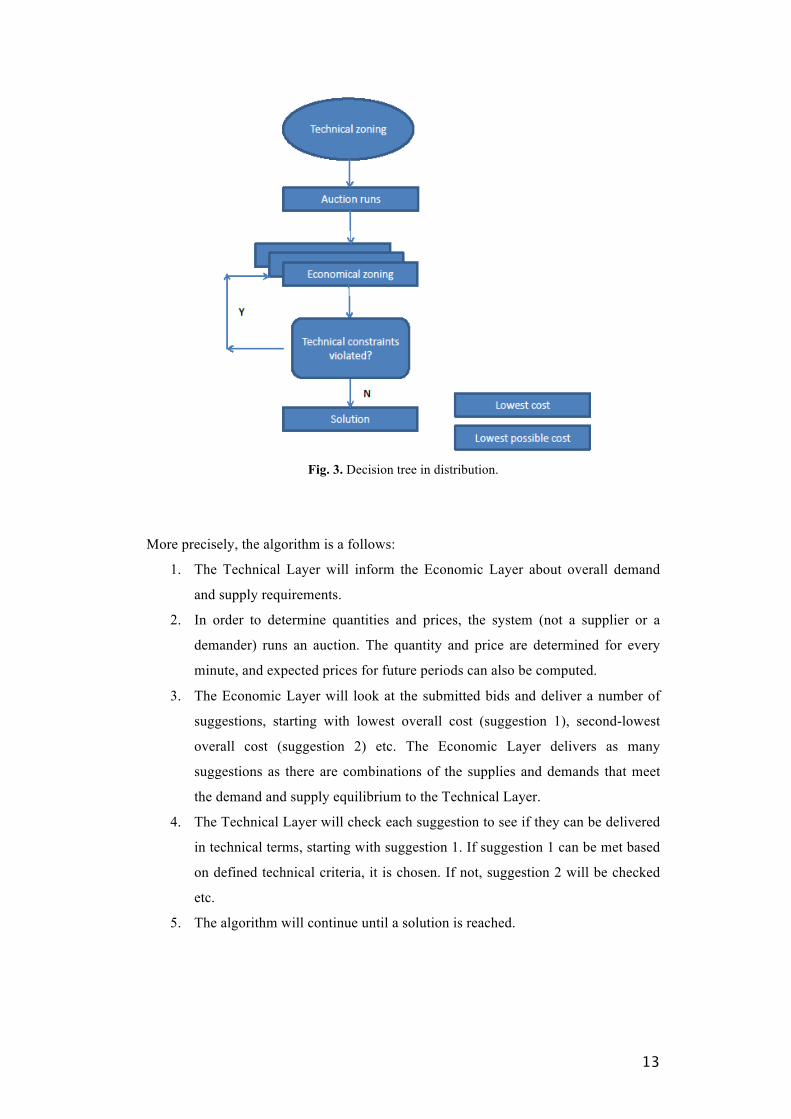
Fig. 3. Decision tree in distribution.

More precisely, the algorithm is a follows:

1. The Technical Layer will inform the Economic Layer about overall demand

and supply requirements.

2. In order to determine quantities and prices, the system (not a supplier or a

demander) runs an auction. The quantity and price are determined for every

minute, and expected prices for future periods can also be computed.

3. The Economic Layer will look at the submitted bids and deliver a number of

suggestions, starting with lowest overall cost (suggestion 1), second-lowest

overall cost (suggestion 2) etc. The Economic Layer delivers as many

suggestions as there are combinations of the supplies and demands that meet

the demand and supply equilibrium to the Technical Layer.

4. The Technical Layer will check each suggestion to see if they can be delivered

in technical terms, starting with suggestion 1. If suggestion 1 can be met based

on defined technical criteria, it is chosen. If not, suggestion 2 will be checked

etc.

5. The algorithm will continue until a solution is reached.

14

5. An example

The network used to illustrate the proposed approach is shown in Fig. 49, with bidding

supplies and demands marked as S and D. The network is a modified version of an

existing UK network considering anticipated changes in 2050 such as:

• Increased Complexity. Reverse power flow is more likely to occur as a result of

the large penetrations of distributed generation and energy storage. The topologies of

networks will be more complex due to the increasing use of soft open points i.e. power

converter devices that are able to regulate active and reactive power flows between

interconnected lines, and potentially more frequent network reconfigurations.

• Increased Uncertainty. Load and generation profiles are expected be more

volatile and less predictable calling for the adoption of new techniques such as real

time thermal rating and demand side response (DSR).

• Increased size. Networks with larger sizes or in larger geographic areas need to

be considered especially as the numbers of controllable devices will increase and with

it the need for enhanced observability and measurements.

• Increased Decentralisation and Active Participation. Future distribution networks

are likely to be more decentralised due to the increasing number of distributed

generation, microgrids, virtual power plants and community energy systems. More

customers are expected to participate in the form of DSR and as producers.

9  This is a modified version of an 11kV UK distribution network. It consists of two primary substations and four 11kV feeders. Energy storage systems, soft open points and distributed generation has been included in order to simulate a future network configuration. D1-D6 are single or aggregated loads. S1, S3, S4 and S5 are individual supplies rated at 10MVA, 5MVA, 7.5MVA and 22.5 MVA respectively. S2 is a 2.5MVA/6 MWh energy storage system. Soft Open Points (SOP1-3) are rated at 3.5MVA each. They are used to regulate power flows between their end-points to satisfy requirements that could be triggered by events during network operation and/or as a result of power set-points suggested by auctions.  

15

Fig. 4. The Technical Layer checks the set-points for feasibility, 11 kV network.

In the network considered there are two obvious zones of control: Control zone A and

Control zone B, in this case interconnected by means of three soft open points (SOP1-3).

We define SOPs according to Cao et al. (2016, p.36): ‘Soft Open Points (SOPs) are

power electronic devices installed in place of normally-open points in electrical power

distribution networks. They are able to provide active power flow control, reactive power

compensation and voltage regulation under normal network operating conditions, as well

as fast fault isolation and supply restoration under abnormal conditions’. In a future

16

scenario of enhanced renewables penetration these Zones could refer to communities that,

although connected to the main grid through the 33/11kV substations, would operate in a

way that could result in demand being satisfied by local generation. This could be driven

by the need to absorb low carbon energy locally to avoid transmission losses, or due to

the fact that the in the future the substations would have reached their nominal capacity;

therefore, instead of network reinforcements, Operators have deployed ‘smart’ solutions

like energy storage and DSR schemes implemented through market operations.

Although the boundaries in the example, between technical zones are obvious i.e.

Control zone A and Control zone B, a similar approach to the one followed in Alimisis

and Taylor (2015) and described in the previous section can be followed to determine the

optimal zoning from a technical perspective10 in more complicated networks resulting in

any number of control zones. Although in this particular case these result in the obvious

zones depicted in Fig. 4, they can also be used if more complex networks are to be zoned.

In terms of the actual power exchange this is practically unregulated i.e. power can

flow between any supplier and any consumer, provided this is technically feasible from a

network operation perspective, as long as total supply always meets the total demand.

Priority will be given for this power equilibrium to be maintained locally i.e. breakers

B1-B5 and SOP1-SOP3 operation will be co-ordinated in a way that results in minimum

power being exchanged with the 33kV network. From an economic point of view we can

assign any demand to meet any supply and therefore economic zones can be determined

from a cost optimisation point of view. However, this will result in the issuing of set-

points inside the technical zone, therefore, new zone suggestions must also fulfil

technical criteria such as line and SOP ratings.

Now, we will show how our Economic and Technical Layers work. An example is

given. Suppose our area is built up in two zones of control –Control zone A and B (initial

zones are the last period’s optimal power flow), where there are 11 bidders participating

in the auction – six demands (D1-D6) and five suppliers (S1-S5)11. Three demands and

four suppliers are in Control zone A and three demands and one supplier in Control zone

B. Suppose the initial zoning structure is set where power flow is optimised. Assume the

Technical Layer has informed the Economic Layer that overall demand in Control zone A

is 12.5 MW and 10 MW in Control zone B. The initial Economic Zones will match the

Control zones as shown in Fig. 4. Table 1 shows the submitted offers and bids in

10  This analysis is beyond the scope of this work. In this paper we base our technical zoning on the criteria suggested in Alimisis and Taylor (2015), which refer to Controllability inside the zone, Interdependency between zones and Relative Size of zones.  11 For example, S1 and S3 could be individual suppliers, S3 and S5 renewable generators, and S2 storage facilities.

17

Economic zone A. For example, the table shows that Demand 1 has submitted a WTP of

120 pence for 5 MW (for 1 minute). The auction is resolved for each minute.

Table 1: Submitted offers and bids in Economic zone A

Demand MW Cost (pence/MW)

Demand 1 5 120

Demand 2 2.5 100

Demand 3 5 90

Suppliers MW Cost (pence/MW)

Supplier 1 2.5 140

Supplier 2 5 130

Supplier 3 7.5 130

Supplier 4 12.5 90

Supplier 4 2.5 80

Table 1 shows that Supplier 4 has submitted two separate bids: a bid to deliver 12.5

MW at a price of 90 pence; and a bid to deliver 2.5 MW at a price of 80 pence. Since we

are in an environment of many demands and suppliers, take the bid to deliver 12.5 MW

and suppose, for example, that Supplier 4 is an aggregation of 13 smaller suppliers - 12

have submitted a bid of 1 MW and one has submitted a bid of ½ MW, all MWs at a price

of 90 pence/MW. Other suppliers and demanders could be seen in a similar way.

Using a two-sided uniform-price auction12, Supplier 4 delivers 12.5 MW to Demands 1,

2 and 3 at a price of 90 pence. Before using the flexible zoning structure, the cost in

Economic zone A alone would be 1125 pence (12.5 MW*90 pence).

Table 2 shows the offers and bids in Economic zone B.

Table 2: Submitted offers and bids in Economic zone B

Demand MW Cost (pence/MW)

Demand 4 5 80

Demand 5 2.5 50

Demand 6 2.5 40

12 A uniform-price auction is a multiple object format, where the price is found at the intersection point of the supply and demand curve (Krishna, 2009).

18

Suppliers MW Cost (pence/MW)

Supplier 5 12.5 50

Supplier 5 10 40

Supplier 5 10 40

Again, using a two-sided uniform-price auction Supplier 5 delivers 10 MW to

Demands 4, 5 and 6 at a price of 40 pence. At this price, the energy cost in Economic

zone B alone would be 400 pence (10 MW*40 pence). Together with Economic zone A,

total energy cost would be 1525 pence.

Now, suppose that Supplier 5’s submitted bid of 12.5 MW can be delivered to

Economic zone A at a price of 50 pence and Demand 5 can placed in Economic zone A

and Demand 2 in Economic zone B. Imagine that the zoning structure re-configures to

include Supplier 5 in zone A, Demand 5 in zone A and Demand 2 in zone B. Now, for

zone A and B, we have Table 3 and 4.

Table 3: Submitted offers and bids in Economic zone A after a re-configuration

Demands MW Cost (pence/MW)

Demand 1 5 120

Demand 3 5 90

Demand 5 2.5 50

Suppliers MW Cost (pence/MW)

Supplier 1 2.5 140

Supplier 2 5 130

Supplier 3 7.5 130

Supplier 4 12.5 90

Supplier 4 2.5 80

Supplier 5 12.5 50

Table 4: Submitted offers and bids in Economic zone B after a re-configuration

Demands MW Cost (pence/MW)

Demand 2 2.5 100

Demand 4 5 80

Demand 6 2.5 40

19

Suppliers MW Cost (pence/MW)

Supplier 5 10 40

Supplier 5 10 40

In line with this the Economic Layer delivers the following two new suggestions to the

Technical Layer, in addition to the result of the initial zoning. The first, in Table 5,

reflects the results of Tables 3 and 4.

Table 5: Suggestion 1 – lowest overall cost

Zones MW Cost (pence/MW)

Economic Zone A (new zone)

Demand 1 5 120

Demand 3 5 90

Demand 5 2.5 50

Supplier 5 12.5 50

Economic Zone B (new zone)

Demand 2 2.5 100

Demand 4 5 80

Demand 6 2.5 40

Supplier 5 10 40

Total cost 102513

The Economic Layer has suggested a lowest cost of 1025 pence. To suggest the

second-lowest overall network cost, the Economic Layer places one of Supplier 5’s

submitted bids of 10 MW in Economic zone A, Demand 2 and Demand 4 in Economic

zone A and Demand 3 and Demand 5 in Economic zone B. Now, for Economic zones A

and B, we have Table 6 and 7.

Table 6: Submitted offers and bids in Economic zone A after a second re-configuration

Demands MW Cost (pence/MW)

Demand 1 5 120

Demand 2 2.5 100

Demand 4 5 80

13 12.5*50+10*40 = 625+400= 1025 pence.

20

Suppliers MW Cost (pence/MW)

Supplier 1 2.5 140

Supplier 2 5 130

Supplier 3 7.5 130

Supplier 4 12.5 90

Supplier 4 2.5 80

Supplier 5 10 40

Table 7: Submitted offers and bids in Economic zone B after a second re-configuration

Demands MW Cost (pence/MW)

Demand 3 5 90

Demand 5 2.5 50

Demand 6 2.5 40

Suppliers MW Cost (pence/MW)

Supplier 5 12.5 50

Supplier 5 10 40

This second reconfiguration gives rise to a new suggestion from the economic layer

shown in Table 8.

Table 8: Suggestion 2 – second-lowest overall cost

Zones MW Cost (pence/MW)

Economic Zone A (new zone)

Demand 1 5 120

Demand 2 2.5 100

Demand 4 5 80

Supplier 4 2.5 80

Supplier 5 10 40

Economic Zone B (new zone)

Demand 3 5 90

Demand 5 2.5 50

Demand 6 2.5 40

Supplier 5 10 40

21

Total cost 140014

The Economic Layer has now delivered three suggestions – a lowest cost of 1025

pence, a second-lowest cost of 1400 pence and the initial zoning structure at a cost of

1525 pence.

Now, the Technical Layer checks the set-points for feasibility. Suggestion 1 results in

supply S5 increasing its power output as a response of a request generated in a different

zone i.e. Control Zone A. Furthermore S1-4 would need to re-adjust their outputs to meet

the demand that is not participating in the auction. This in essence constitutes a re-

configuration of the control zones. As S5 now provides power to all Demands

participating in the auction this could now result in two different zones of Control as

shown in Fig. 5a, provided controllability is maintained using flexibility provided by

assets such as the SOPs. However, based on power flow calculation, in this conceptual

example this would result in the power between the two zones exceeding the nominal

capacity of SOP1. Hence, the Technical Layer rejects Suggestion 1. Suggestion 2 is

examined which results in the zoning shown in Fig. 5b. As there is no exceeding of

technical constraints throughout the network, Suggestion 2 is therefore feasible.

Suggestion 2 is accepted by Technical Layer.

(a) (b)

Fig. 5 Suggested zones after re-configuration a) Suggestion 1 b) Suggestion 2. The reader

is encouraged to refer to section 4 paragraph 2, above, for a definition of control and

economic zones.

14 12.5*80+10*40 = 1000+400= 1400 pence.

T1T2T3

Bus2Bus4

Bus3Bus5

G

Bus6

DG1  Bus

Bus8Bus9

Bus10Bus12

GBus11

Bus14Bus15

Bus17

Bus20

Bus21

Bus23

Bus24

Bus25

Bus28

Bus26Bus27

Bus29

Bus41

Bus33

Bus36

Bus38

Bus34 Bus39

Bus40

T1T2T3

Bus2Bus4

Bus3Bus5

G

Bus6

Bus8Bus9

Bus10Bus12

G

Bus11

Bus14Bus15Bus16

Bus17

Bus20

Bus21

Bus23

Bus24

Bus25

Bus28

Bus26Bus27

Bus29Bus36

Bus38

Bus34 Bus39

Bus40

~ ~

~ ~

~ ~

SOP1

SOP2

SOP3

B1 B2B3

G

Bus41

Bus42

Bus43Bus44

Bus45 Bus46Bus47

Bus48Bus49

Bus50

Bus51 Bus52

Bus53 Bus54

Bus55 Bus56

D1

D2D4

D3 D5

D6

Bus38Bus34

S1

S2

S3

S4 S5

B4 B5

Control  zone  A

Control  zone  BControl  zone  boundary

Economic  zone  A

Economic  zone  B

Exceeding  of  rated  power

T1T2T3

Bus2Bus4

Bus3Bus5

G

Bus6

DG1  Bus

Bus8Bus9

Bus10Bus12

GBus11

Bus14Bus15

Bus17

Bus20

Bus21

Bus23

Bus24

Bus25

Bus28

Bus26Bus27

Bus29

Bus41

Bus33

Bus36

Bus38

Bus34 Bus39

Bus40

T1T2T3

Bus2Bus4

Bus3Bus5

G

Bus6

Bus8Bus9

Bus10Bus12

G

Bus11

Bus14Bus15Bus16

Bus17

Bus20

Bus21

Bus23

Bus24

Bus25

Bus28

Bus26Bus27

Bus29Bus36

Bus38

Bus34 Bus39

Bus40

~ ~

~ ~

~ ~

SOP1

SOP2

SOP3

B1 B2B3

G

Bus41

Bus42

Bus43Bus44

Bus45 Bus46Bus47

Bus48Bus49

Bus50

Bus51 Bus52

Bus53 Bus54

Bus55 Bus56

D1

D2D4

D3 D5

D6

Bus38

Bus34

S1

S2

S3

S4 S5

B4 B5

Control  zone  B

Control  zone  A

Control  zone  boundary

Economic  zone  A

Economic  zone  B

22

6. Discussion

We have shown that locational marginal prices (LMPs), auctions and our flexible zones

could be the way towards a lowest cost electricity system. Importantly, our set-up can

improve on the outcome in a world of pre-defined, fixed and/or static electricity

networks. That said, there could be a mismatch between the lowest system cost, and what

is possible taking into account control and operation is. Using economics to drive zone

re-configuration could result in drastic changes in the setting of control zones, however,

provided the enhanced flexibility offered by assets in 2050 we have shown that this could

be a viable option.

The use of zones can be analysed three ways: (1) only in terms of control and operation

without taking into account the economics when determining zones; (2) only in terms of

economics without taking into account the control and operation technique when

determining zones; (3) a mix between control and operation and economics when

determining zones.

Approach (1) is analysed in Alimisis et al., (2013) and Piacentini et al., (2013), (2) is

an alternative approach to the problem and approach (Krishna, 2009) (3) is the most

desirable scenario, and what has been analysed in this paper.

6.1. Feasibility

One might wonder whether or not our economic set up could be used after an

optimisation of control and operation. The answer is yes. The control and operation set

boundaries for the power flow. If the Technical Layer allows room for lower overall cost,

our algorithm aims to find it. If not, we already have the lowest possible cost. In any case,

the market (boundaries and bidders) decides which configuration ensures lowest feasible

cost.

6.2. Number of zones

Then we may ask: What is the minimum/maximum number of zones? Following the

discussion above, the minimum or maximum number of zones is determined by the

Technical and Economic Layers. The Economic Layer will determine prices and

therefore, who are the cheaper suppliers. The Technical Layer determines the number of

zones. The number zones depend on bids, demand and constraints.

23

7. Extensions

In this paper, we presented a method that can secure a lowest cost in a system made up

of many local power zones. Our zoning structure reacts if the control and operation

allow/require it. However, this does not necessarily suggest that it should be like this.

There could be a welfare improvement and lower cost by letting control and operation

follow the economics. A further extension could be to take the technical part of this paper

and look at it through a Multi-Agent System (Cameron et al. 2015) at the distribution

level and add economics. The aim of such a follow-on paper should be to demonstrate

that network conditions, including market constraints and considerations, can be used not

only to determine the most appropriate control and communication architecture from a

technical perspective, but also to trigger architectural changes in the Technical Layer in

order to maximize economic benefits.

References AER (2011). National Electricity Market. Australian Energy Regulator.

Alimisis V, Piacentini C, King J, Taylor P. (2013). ‘Operation and Control Zones for

Future Complex Power Systems’, in Green Technologies Conference, IEEE, pp. 259-265.

Alimisis, V. and Taylor, P. (2015). ‘Zoning Evaluation for Improved Coordinated

Automatic Voltage Control’, IEEE Transactions on Power Systems, 30(5), pp. 2736-

2746.

Binetti, G., Davoudi, A., Naco, D., Turchiano, B. and Lewis, F. (2014). ‘A Distributed

Auction-Based Algorithm for the Nonconvex Economic Dispatch Problem’, IEEE

Transactions on Industrial Informatics, 10(2), pp. 1124-1132.

Cameron, C., Patsios, C., and Taylor, P. (2015). ‘On the benefits of using self-

organising Multi-Agent architectures in network management’, In Smart Electric

Distribution Systems and Technologies (EDST), 2015 International Symposium, pp. 335-

340).

Cao, W., Wu, J., Jenkins, N., Wang, C., Green, T. (2016), ‘Operating principle of Soft

Open Points for electrical distribution network operation’, Applied Energy, 164, pp. 245-

257.

Chai, S. and Sekar, A. (2001). ‘Graph theory application to deregulated power system’,

In System Theory, 2001. Proceedings of the 33rd Southeastern Symposium, pp. 117-121.

Chen W-K. (1997). ‘Graph Theory and Its Engineering Application’, World Scientific.

DECC (2013). Smart Metering Implementation Programme, London: DECC.

24

ENA (2015). Engineering Report 3 Issue 1 2015 Climate Change Adaptation

Reporting Power Second Round, London: ENA.

FERC (2012). Energy Primer: A Handbook of Energy Market Basics, Washington:

FERC.

Frontier Economics (2009). Generator Nodal Pricing – a review of theory and

practical application, . Frontier Econonics.

Hogan W. (2002). ‘Electricity Market Restructuring: Reforms of Reforms’, Journal of

Regulatory Economics, vol 21(1) pp. 103-132.

Groomes PE and Rustum J. (2013). Electricity regulation in the United States:

Overview. Thomson Reuters.

Krishna V. (2009). Auction Theory, San Diego: Academic Press.

McArthur S, Taylor P, Ault G, King J, Athanasiadis D, Alimisis V and Czaplewski

M. (2012). ‘The Autonomic Power System – Network Operation and Control Beyond

Smart Grids’ In 2012 3rd IEEE PES Innovative Smart Grid Technologies Europe (ISGT

Europe), pp. 1-7.

Newbery D. (2006) ‘Market Design’. Working Paper, University of Cambridge.

Piacentini C, Alimisis V, Fox M, Long D. (2013). ‘Combining a Temporal Planner

with an External Solver for the Power Balancing Problem in an Electricity Network’,

In ICAPS.

PJM (2014a). PJM Annual Report, Audubon: PJM.

PJM (2014b), Power System Fundamentals, Audubon: PJM.

Thomas AR, Lendel I and Park S. (2014). Electricity Markets in Ohio, Center for

Economic Development and Energy Policy Center: Ohio.