Cambridge-INET Working Paper Series No: 2014/06

Cambridge Working Paper in Economics: 1455

WINNING THE OIL LOTTERY:

THE IMPACT OF NATURAL RESOURCE

EXTRACTION ON GROWTH

ABSTRACT

This paper provides evidence on the causal impact of oil discoveries on local development. Novel data on the drilling of 20,000 oil wells in Brazil allows us to exploit a quasi-experiment: municipalities where oil was discovered constitute the treatment group while municipalities with drilling but no discovery are the control group. The results show that oil discoveries significantly increase per capita GDP and urbanization. We find positive spillovers to non-oil sectors, specifically an increase in services GDP which stems from higher labor productivity. The results are consistent with greater local demand for non-tradable services driven by highly paid oil workers.

Tiago Cavalcanti Daniel Da Mata Frederik Toscani (University of Cambridge) (University of Cambridge) (University of Cambridge)

Cambridge-INET Institute

Faculty of Economics

Winning the Oil Lottery:

The Impact of Natural Resource Extraction on Growth∗

Tiago Cavalcanti† Daniel Da Mata‡ Frederik Toscani§

Version: March 10, 2014.

Abstract

This paper provides evidence on the causal impact of oil discoveries on local

development. Novel data on the drilling of 20,000 oil wells in Brazil allows us to

exploit a quasi-experiment: municipalities where oil was discovered constitute the

treatment group while municipalities with drilling but no discovery are the control

group. The results show that oil discoveries significantly increase per capita GDP and

urbanization. We find positive spillovers to non-oil sectors, specifically an increase in

services GDP which stems from higher labor productivity. The results are consistent

with greater local demand for non-tradable services driven by highly paid oil workers.

Keywords: Petroleum Industry, Economic Growth, Urbanization

JEL Classification: O13, O40

∗We have benefited from discussions with Toke Aidt, Francesco Caselli, Silvio Costa, Jane Fruehwirth,Sriya Iyer, Pramila Krishnan, Hamish Low, Sheilagh Ogilvie, Andre Pereira, Cezar Santos, Rodrigo Serra,Edson Severnini, Claudio Souza, Daniel Sturm, and Jose Tavares. Frederik Toscani gratefully acknowledgesthe hospitality of PUC-Rio de Janeiro where part of the work on this paper was done. We thank the KeynesFund, University of Cambridge, for financial support. All remaining errors are ours.

†Faculty of Economics, University of Cambridge.‡IPEA.§Faculty of Economics, University of Cambridge.

1

“No other business so starkly and extremely defines the meaning of risk and reward -

and the profound impact of chance and fate.” Yergin (2008)

1 Introduction

Natural resource extraction influences a myriad of economic factors ranging from political

economy to fiscal and monetary policy. However, no clear consensus has emerged on

whether economies which discover natural resources should anticipate prosperous times or

fear the much discussed Dutch Disease. Disentangling the various channels through which

natural resources affect the economy has proven challenging. Even the pure market effect

of natural resource extraction is not well understood. Natural resource extraction might

crowd out other sectors of the economy by driving up local prices, or on the other hand

could have positive spillovers which lead to the concentration of economic activity.

This paper uses the quasi-experiment generated by the random outcomes of exploratory

oil drilling in Brazil in order to investigate the causal effect of natural resource discoveries

on local development.1 Specifically, we compare economic outcomes in municipalities where

the national oil company Petrobras drilled for oil but did not find any, to outcomes in those

municipalities in which it drilled for oil and was successful.2 Drilling attempts were carried

out in many locations with similar geological characteristics, but oil was found in only a few

places. The “treatment assignment” is related to the success of drilling attempts: places

where oil was found were assigned to treatment, while places with no oil are part of the

control group. The treatment assignment resembles a “randomization” since (conditional

on drilling taking place) a discovery depends mainly on luck. Therefore, places with oil

discoveries are the “winners” of the “geological lottery”. Since there were no significant

royalty payments to municipalities in Brazil until several decades after the first discoveries,

we are able to isolate the direct impact of oil extraction from the effect of fiscal windfalls.

Our analysis uses a novel dataset on the drilling of approximately 20,000 oil wells in

Brazil from 1940-2000. The dataset covers the complete universe of wells drilled since

exploration began in the country and provides information on three stages regarding oil

extraction and production: drilling, discovery, and upstream production. We use this

detailed information on the data generating process to distinguish those municipalities

which were assigned to treatment from those which constitute the control group. Our focus

1Oil and gas are also called petroleum or hydrocarbons. Throughout this paper we use “oil” to refer to“oil and gas”. The oil industry is loosely divided into two segments: upstream and downstream. Upstreamrefers to exploration and production of oil while downstream refers to processing and transportation(refineries, terminals etc).

2There are three administrative levels in Brazil: federal government, states, and municipalities. Mu-nicipalities are autonomous entities that are able, for instance, to set property and service taxes. They areroughly equivalent to counties in the US. We use the words municipalities, local governments and localeconomies interchangeably.

2

is on an Intent-to-Treat (ITT) analysis where we regress our outcome variables of interest

directly on discoveries. Discoveries take place in different locations over time, so we can

exploit time and cross-sectional variations. The ITT analysis enables us to obtain a lower

bound for the average treatment effect. We also estimate a Local Average Treatment Effect

(LATE) by instrumenting for production with discoveries.3 Besides, we study treatment

intensity using detailed information on different types of wells. This allows us to retrieve

a coefficient that can be interpreted as a weighted-average of per-unit treatment effect.

The baseline results show that locations which discover oil have a 24.6-25.9% higher per

capita GDP over a span of up to 60 years compared to the control group. Furthermore, we

document an increase in both manufacturing and services GDP per capita but no impact

on agricultural GDP. While the measure of manufacturing GDP includes natural resource

extraction (and as such an increase is not surprising), the increase in services indicates

spillover effects of oil production impacting the rest of the economy.4 Additionally, we find

evidence for an increase in urbanization of about 4% points. This increase in urbanization

is consistent with the increase in services we document. We do not find any effect on

population density. Using historical data on sectoral employment we calculate a measure

of sectoral labor productivity and show that oil discoveries increase GDP mainly by in-

creasing productivity and not by increasing employment. We also show that while both

onshore and offshore discoveries increase manufacturing GDP (potentially in a mechanical

way since it includes oil production), only onshore discoveries increase services GDP and

urbanization. We hypothesize that demand from well paid oil workers are responsible for

the observed increase in services and urbanization. Oil municipalities become local service

and commerce hubs which benefit from improved labor productivity.5 The treatment in-

tensity analysis suggests that major discoveries have a disproportionately large impact on

the local economy.

The fact that we do not find a positive impact on population and employment density

on average might be due to the concentration of the oil industry in Brazil: the U.S. has a

more widespread ownership of resources than Brazil. There are thousands of oil companies

in the U.S. in contrast to the historical monopoly of Petrobras in Brazil. Due to this

market structure oil services are more likely to be concentrated in just a few places in

Brazil. By contrast, in the U.S. an entire chain of small oil services can be located close

to the more widespread oil firms.

3Endogeneity of production might be more of a problem for gas than for oil. While it is relatively easyto transport oil, gas requires a substantial investment in infrastructure such as pipelines.

4Oil discoveries and production might have a positive or negative impact on non-oil manufacturing.Given the data constraints we cannot investigate this, unfortunately.

5A recent report from the McKinsey (2013) Global Institute highlights the importance of oil and gasexploration and production on economic development by supporting local employment and supply chains.It argues that in many countries revenues spent on local goods and services often exceed tax and royaltypayments.

3

Our results are robust to a variety of control groups, different control variables, and

a restriction of the sample period to 1940-1996. The latter is important since from 1997

onwards royalty payments became an important part of municipal income. By restricting

the analysis to the period prior to 1997 we verify whether our results are driven by di-

rect market effects or operate indirectly via government windfalls. Lastly, we show that

municipalities with oil discoveries have a higher probability of hosting major downstream

oil facilities than the control group. To check whether our results are driven by these

downstream facilities we re-run the regressions excluding those municipalities which host

them and find that this is not the case. It appears that upstream production does not only

impact the local economy via downstream production but has also a direct effect.

Since the Oil and Gas industry is at the center of the production network in many

countries, its impact on the economy has been studied extensively in the literature. The

usual approach to disentangle the effects of oil production relies on cross-country evidence.

Several papers in the literature have shown correlations between natural resources and ad-

verse outcomes. For instance, Sachs and Warner (1995) show that resource-exporting coun-

tries tend to have lower growth rates, while Isham, Woolcock, Pritchett, and Busby (2005)

point out that resource-exporting countries have poorer governance indicators. However,

cross-country evidence is sensitive to changing periods, sample sizes, and covariates (see

van der Ploeg (2011) for an overview of the literature)6. Additionally, cross-country stud-

ies usually use very aggregate variables and make it difficult to control for institutional

and cultural frameworks, and for policy variation between different countries.

As a result, the literature has been shifting attention to a more detailed analysis to

pin down specific mechanisms of how natural resources impact the economy. The main

empirical challenge, however, is to deal with the issue of endogeneity of natural resource

extraction since there are many unobservable variables that might be correlated with oil

production and might also affect economic development. Notable papers in an emer-

gent literature which tries to address these problems more directly are, among others,

Allcott and Keniston (2013), Caselli and Michaels (2013), Monteiro and Ferraz (2012), and

Michaels (2011)7. While Allcott and Keniston (2013) and Michaels (2011) focus on the

US we study a developing country8. More importantly, while the above papers are close

6There is also a large theoretical literature which tries to explain how natural resource abundance mightaffect economic outcomes, such as theories based on the Dutch Disease hypothesis (e.g., Corden and Neary(1982) and Krugman (1987)) or rent-seeking theories (e.g., Lane and Tornell (1996) and Caselli and Tesei(2011)).

7Also see Acemoglu, Finkelstein, and Notowidigdo (2009) and Dube and Vargas (2013).8Caselli and Michaels (2013) and Monteiro and Ferraz (2012) also investigate the impact of oil using

data from Brazilian municipalities. Our paper differs from theirs not only methodologically but alsoregarding the question and the time span. Caselli and Michaels (2013) focus on the effects of oil windfalls(Royalties) on government behavior and the provision of public goods, while Monteiro and Ferraz (2012)also use Royalties to study local political and economic outcomes. We study the direct effects of oildiscoveries instead of the indirect effect via royalties.

4

in spirit to our exercise we are, to our knowledge, the first to identify the impact of

oil using the entire track of oil discoveries, since the existing literature mainly limits

attention to post-discovery periods. This paper is the first to estimate the impact of

oil discoveries on local economic development using a (quasi-experimental) difference-in-

difference design. In terms of design and results our paper is also related to the litera-

ture on agglomeration externalities, especially the branch which investigates the impact

of interventions on the concentration of economic activity (Davis and Weinstein (2002),

Greenstone, Hornbeck, and Moretti (2010)). Similarly to our research, these papers are

motivated by the insights about the importance of within-country differences in out-

put and wages (see Acemoglu and Dell (2010) and Moretti (2011)). Lastly, our focus

on sectoral GDP links the paper to studies on the determinants of structural transfor-

mation, particularly the ones focusing on the role of the oil sector (Stefanski (2010),

Kuralbayeva and Stefanski (2013), Gollin, Jedwab, and Vollrath (2013)).

While our results are derived for a specific institutional framework we believe that

some general lessons can be drawn from our empirical exercises. Specifically, being able to

address issues of endogeneity and unobservable variables allows us to make causal state-

ments. Our results are consistent with the view that oil abundance is not necessarily a

curse at the local level. It is important to stress, however, that we cannot comment on

the aggregate impact of oil discoveries on the country as a whole. Compared to national

economies, municipalities are much more open and face macroeconomic policies which are

invariant to their idiosyncratic conditions. By construction our research design rules out

any effect which operates through the nominal exchange rate, for example.

This article proceeds as follows. Section 2 provides the background on oil drilling and

on the key institutional aspects of oil exploration and production in Brazil. Section 3

details the research design used to identify the impact of oil on economic development.

In this paper we combine several datasets which are detailed in a subsection of Section

3. Section 4 discusses the estimation strategy. Section 5 shows the results and robustness

exercises. Section 6 concludes.

2 Background

2.1 Oil Drilling

Oil and Gas exploration is a risky business. Oil companies aim to find an oil field, which

corresponds to a contiguous geographic area with oil. Oil companies search for areas with

specific geological characteristics to drill for oil. For instance, oil companies search for areas

that contain geological structures (subsurface contortions and specific rocks) for potential

trapping of hydrocarbons. Based on geological, geophysical, and geochemical information,

5

an oil company selects an area to drill for oil. Geology and related disciplines provide

guidance on where to search for oil traps and estimating the probability of discovery prior

to drilling is an important aspect of petroleum exploration. However, only by drilling can

the company be certain that hydrocarbon deposits really exist. In other words, the only

direct way of confirming the hypothesis of oil presence is by drilling a well. Even with

modern technology, it is only by drilling that the existence of oil can be confirmed. Oil

companies may invest substantially in acquiring information to end-up with no discoveries

or no profitable discoveries.

When an oil company drills a hole, the wells are classified according to the results of

the attempt. A drilled well can be classified, among other categories, as a discovery well,

a producer well, a dry hole, or an abandoned well (e.g., because of an accident). The

likelihood of finding oil from drilling can be low even in areas with appropriate geological

characteristics and learning-by-doing is an important aspect in the petroleum industry

(Kellogg (2011)). Testing by drilling is expensive and may not reduce the uncertainty

regarding the existence of oil. Numbers vary but in a newly explored area the likelihood of

drilling for oil successfully can be very low and subjective probabilities are widely accepted

in the petroleum industry (Harbaugh, Davis, and Wendebourg (1995)). Today, an explo-

ration well (wildcat well9) can have a probability as low as 10% of finding viable oil, while

a rank wildcat10 has an even smaller chance of finding oil. Therefore, even with modern

technology, drilling is not a “safe bet” since there is no guarantee that a company will find

oil after drilling. Given the features of drilling, oil discovery depends both on geological

characteristics and on “luck”11. Our data support the idea that discovering oil is sort of

a “lottery”: for every exploration well drilled which was successful there were many more

unsuccessful ones.

A myriad of factors influence drilling success such as past drilling history, regional

endowment, resource depletion, onshore or offshore drilling, and technological progress.

While not immediately relevant for our research design it is worth pointing out that two of

those factors changed during our period of analysis: the level of technology available and

the availability of conspicuous targets of hydrocarbon deposits. A more detailed discussion

of oil drilling is given in Appendix B.

2.2 Oil in Brazil

Our period of analysis is from 1940 to 2000. Under most of this period, only government-

owned entities were able to explore and produce oil in Brazil. In 1938, under a dictatorship

9A well drilled a mile or more from an area of existing oil production.10A well drilled in an area where there is no existing production.11According to Harbaugh, Davis, and Wendebourg (1995), “luck is obviously a major factor in explo-

ration”.

6

period (1937-1945), Federal Law n. 395/38 established the state control of oil development

and only by 1997 (Federal Law n. 9,478/97) private companies would be allowed to au-

tonomously explore and produce oil in Brazil. Federal Law n. 395/38 created the CNP

(In Portuguese, Conselho Nacional do Petroleo), the only entity responsible for exploring

oil from 1938 to 1953.12 Afterwards, from 1953 to 1997, only one company was allowed to

drill for oil in Brazil: the government-controlled Petrobras13. Petrobras is an integrated

exploration and production company whose activities reach all phases of the oil supply

chain. To be precise, under certain circumstances other oil companies could explore oil in

Brazil, but only in partnership with Petrobras. Following the oil crisis in 1973, Petrobras

and other oil companies could sign a so-called “risk contract” to explore specific areas be-

tween 1975 and 1987. The terms of the contracts varied, but usual aspects included that

the oil found under this type of contract could not be exported and that Petrobras could

explore simultaneously an adjacent area by itself14. There is a sharp contrast in terms of

ownership of resources between the United States in Brazil. There are thousands of oil

companies with various business models in the U.S.15, while Brazil has been historically

linked with Petrobras’s monopoly.

Local governments had little space to influence Petrobras (or CNP) on where to search

for oil and on the speed of drilling. First, Petrobras (as a National Oil Company) fol-

lowed national goals that may be not correlated with local-level objectives. Petrobras

had a long-term goal, namely, achieving Brazil’s self-sufficiency in oil production (inde-

pendent of preferences of the local authorities). Second, several factors which influence

the exploration activity are determined exogenously such as the international price of oil

(Mohn and Osmundsen (2008)). Third, Petrobras knew it could only drill in locations with

selected geological characteristics. One concern might be that Petrobras’ “risk contract”

partners might have been local companies with a local agenda. However, the large ma-

jority of those contracts were signed with profit-maximizing multinational oil companies.

Three smaller Brazilian companies also signed exploration contracts with Petrobras. Out

12According to Federal Law n. 395/38, private oil companies could only operate via concessions givenby CNP. Anecdotal evidence point out that it was difficult to operate in Brazil as a private oil companyat that time.

13Petrobras was created in 1953 by Federal Law n. 2,004/53. In 1954, Petrobras began its explorationactivities. Constitutional Amendment 09/1995 and Federal Law 9,478/97 changed the upstream industryin Brazil: after 1997, the upstream oil market was open to national and foreign oil firms and Petrobrasstarted to face competition. Nowadays, Petrobras is one of the largest oil companies in the world. Petro-bras is a leading company in oil exploration with contributions to technology, especially of deep waterexploration.

14The first contracts were signed in 1976 through a public bidding of 10 areas to explore oil. Out of the10 areas, 9 were offshore and 1 was in the Amazon basin. More than 100 risk contracts were signed during12 years. According to the contracts, if oil was found, it should be sold to the internal market until thecountry reached its self-sufficiency in oil production. Brazil reached its self-sufficiency three decades later,in 2006.

15Institutions such as the U.S. Energy Information Administration and the Independent PetroleumAssociation of America report the existence of several thousand oil operators in the U.S. economy.

7

of these three companies, only one was a government-owned company: the “Paulipetro”

created in 1979 by Sao Paulo state16. Between 1980 and 1983, Paulipetro drilled 33 wells

in one specific area. The drilling attempts lead to only one discovery well, but a non-

economical one (Bosco (2003)). Apart from Petrobras, Paulipetro drilling had support of

other national-level institutions such as the CPRM (Brazil’s Mineral Resource Research

Company). Even guided by state-level goals, Paulipetro attempts were probably not linked

to any local-level (local governments’) influence and either way proved unsuccessful.

The Brazilian oil sector has experienced a substantial development from 1940 onwards.

In 1939 the first onshore field was discovered (but non-commercial) and in 1941 the first

onshore commercial producer well was drilled. The first oil discovery from an offshore well

took place in 1968. In 2011, Brazil was the world’s 13th largest producer of oil and gas

with 2.2 millon barrels per day, which represents 2.6% of the total produced worldwide.

Brazil was the world’s 14th position in terms of proven petroleum reserves in the same

year (ANP (2012)). The size of the oil sector is relevant to the Brazilian economy: in 2011

the oil sector represented 12% of the total Gross Domestic Product (CNI (2012)). Figure

1 summarizes domestic and international events related to oil exploration and production

in Brazil.

The oil business is crucial to several municipalities. Out of the top 10 municipalities

with highest per capita GDP, several of them have their main economic activity associ-

ated with upstream or downstream oil industry. Municipalities in the top 10 list include

Sao Francisco do Conde (with a refinery17), Triunfo (petrochemicals industry), Quissama,

Campos, and Macae (the last three municipalities linked to offshore production). Anecdo-

tal evidence suggests that municipalities which discovered large amounts of oil underwent a

significant transformation and substantial economic growth. For example, Macae, a fishing

municipality, transformed from a rural place to a very urban place after Petrobras discov-

ered offshore oil in the area and located some of its key production facilities in Macae

in the 1970’s. There are also anecdotes of Petrobras hiring hundreds and thousands of

rural workers to join drilling expeditions. In the 1960’s, the municipality of Carmopolis,

located in a historically sugarcane producing area, discovered oil. Since then, Carmopolis

has changed its main business due to the presence of Petrobras and related oil service com-

panies. Carmopolis has presented a high GDP growth even though there are complains

regarding the lack of connection between oil service firms and the community18. The mu-

nicipality of Alagoinhas in Bahia discovered oil in 1964. A number of successive discovery

wells lead Petrobras to locate some of its facilities in Alagoinhas in the late 1960s. Anec-

16Sao Paulo is the largest state in Brazil both in terms of population (22% of the Brazilian totalpopulation in 2010) and gross domestic product (33% of the Brazilian total GDP in 2008).

17The first refinery was constructed in 1949 in the municipality of Sao Francisco do Conde (located inBahia state). The refinery is called RLAM (Refinaria Landulpho Alves-Mataripe) and is located near thevery first wells that discovered oil in the country.

18See http://www.uff.br/macaeimpacto/OFICINAMACAE/

8

dotal evidence suggests that this lead to rapid economic growth in the area, particularly in

the services sector. Alagoinhas became a services hub for the surrounding municipalities

and large commercial outfits located there.19

Figures 2, 3 and 4 show the development of GDP per capita for the period 1940-2000

in the states of Sergipe (onshore production), Rio de Janeiro (offshore production) and

Bahia (first state to discover oil), respectively. For each state, the graphs illustrate the

evolution of GDP of municipalities with and without oil. It can be seen that a wedge in

GDP per capita between oil producing municipalities and those without oil production

emerges over the years. Furthermore, the timing seems to correspond quite closely to the

development of the oil sector in each respective state. At a first pass, oil production thus

seems to substantially increase local GDP. Two questions arise from this. Firstly, is the

observed correlation causal? And secondly, how does the non-oil sector develop? Since oil

extraction is a very high value added activity, local GDP mechanically increase when oil is

produced, bar any extreme “Dutch Disease” effect. We are interested in assessing whether

the spillovers of oil production to other sectors are positive or negative.

An important warning is related to the distribution of oil windfalls. Royalties and other

forms of “government take” are collected from both onshore and offshore oil production.

By and large, a company that produces oil must allocate part of the value of the gross

output in the form of royalties. Royalties are then divided among the three administrative

levels in Brazil. The distribution of royalties started in 1953, but it represented only a very

small fraction of local governments’ budget. Only after 1997 (Federal Law n. 9,496/1997),

did royalties start to represent a significant amount of revenue to local government. In

the robustness exercise, we restrict our analysis to the years 1940-1996 to capture only

the direct effect of oil production rather than the indirect effect through royalties. See

Appendix C for an overview and discussion of Royalties.

In the next section we discuss the identification strategy used to retrieve the effect of

oil discoveries on growth of local economies in Brazil.

3 Research Design

We are interested in the impact of oil discoveries on local economic development. We

study this question by defining the analysis in terms of the treatment evaluation litera-

ture where we see oil production as our treatment of interest and oil discoveries as the

assignment to treatment. In this section, we detail our research design which is based on

exploiting the quasi-random nature of oil discoveries. Our research design exploits un-

confounded assignment and we perform several exercises to guarantee adequate overlap

between the treatment and control group (strong ignorability as in Rosenbaum and Rubin

19See http://pt.wikipedia.org/wiki/Alagoinhas

9

(1983)). While it is common in the literature on natural quasi-experiments to match on

observable variables, our research design additionally provides several strategies to “match

on unobservables”. We start by describing the data and then discuss the exogeneity of

oil discovery and its relation to the treatment assignment. We then turn to the issue of

balance in the covariate distributions between treatment and control groups.

3.1 Data

The data on drilling is from Agencia Nacional do Petroleo, Gas Natural e Biocombustıveis

(ANP), the Brazilian oil and gas industry regulator. The well dataset contains detailed

information on the drilling of 19,493 wells in Brazil spanning from 1940 to 2000. The

dataset contains the latitude and longitude coordinates of the well, so we are able to know

the exact location of each well. The dataset also has information on the exact date of

the drilling, on the result of the drilling (whether oil was found, whether the well is a dry

hole, whether only water was found, or whether the well was abandoned because of an

accident20). Furthermore, we have information on the viability of exploring the oil deposit

(when oil was found), and on whether the oil company started production.

The richness of the well dataset allows us to study several possibilities regarding the

stages of oil extraction and production (upstream oil industry). Given the data, we are able

to separate places where drilling took place (J = 1) from places with no drilling (J = 0).

We can also obtain information on places with oil discoveries (Z) and with oil production

(D). As a first step we created a dummy variable for drilling (J), two different dummy

variables for discovery (Z), and a dummy for well production (D). The dummies for

drilling and production follow immediately from the well data. The drilling dummy equals

one when at least one well was drilled in the municipality and the production dummy is

one when there is at least one producer well in the municipality. In terms of discoveries,

there are several possibilities as the data allow us to differentiate between a field discovery,

a subfield (reservoir) discovery and a field extension discovery. We define two different

discovery dummies as follows. Firstly, “All Discoveries”: the dummy is one when at least

one field, subfield or field extension discovery was made in the municipality. Secondly,

“True Discoveries”: The dummy is one when at least one field or subfield discovery and

at least one field extension discovery was made in the municipality. The rationale for the

latter is that any substantial discovery includes a field or subfield discovery and subsequent

field extension discoveries to delineate the size of the oil field (see Appendix B). For now

20We obtain more the 50 different classifications from the dataset, but we were able to aggregate all ofthem to the following major categories: discovery of a field or subfield (reservoir), extension of a field orsubfield, producer, non-feasible production, dry holes, abandoned, and well used for injection of water,steam or gas. The data differentiate between oil well, gas well, and oil and gas well. One limitation ofthe dataset is that we do not have information on the amount of oil produced by each individual producerwell for the period of interest. Data on well production is available only from the 2000’s onward.

10

we will use the “All Discoveries” dummy to start with the most general possible definition

of discoveries.

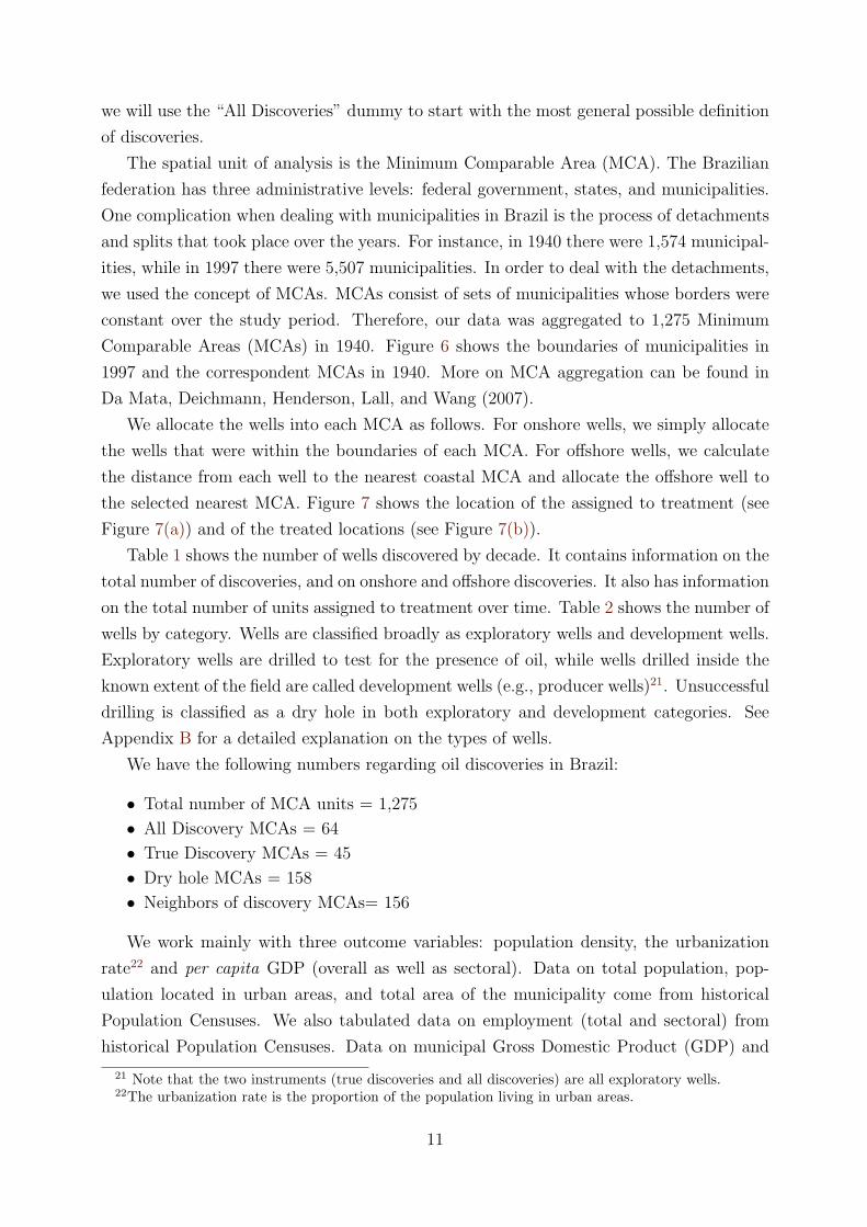
The spatial unit of analysis is the Minimum Comparable Area (MCA). The Brazilian

federation has three administrative levels: federal government, states, and municipalities.

One complication when dealing with municipalities in Brazil is the process of detachments

and splits that took place over the years. For instance, in 1940 there were 1,574 municipal-

ities, while in 1997 there were 5,507 municipalities. In order to deal with the detachments,

we used the concept of MCAs. MCAs consist of sets of municipalities whose borders were

constant over the study period. Therefore, our data was aggregated to 1,275 Minimum

Comparable Areas (MCAs) in 1940. Figure 6 shows the boundaries of municipalities in

1997 and the correspondent MCAs in 1940. More on MCA aggregation can be found in

Da Mata, Deichmann, Henderson, Lall, and Wang (2007).

We allocate the wells into each MCA as follows. For onshore wells, we simply allocate

the wells that were within the boundaries of each MCA. For offshore wells, we calculate

the distance from each well to the nearest coastal MCA and allocate the offshore well to

the selected nearest MCA. Figure 7 shows the location of the assigned to treatment (see

Figure 7(a)) and of the treated locations (see Figure 7(b)).

Table 1 shows the number of wells discovered by decade. It contains information on the

total number of discoveries, and on onshore and offshore discoveries. It also has information

on the total number of units assigned to treatment over time. Table 2 shows the number of

wells by category. Wells are classified broadly as exploratory wells and development wells.

Exploratory wells are drilled to test for the presence of oil, while wells drilled inside the

known extent of the field are called development wells (e.g., producer wells)21. Unsuccessful

drilling is classified as a dry hole in both exploratory and development categories. See

Appendix B for a detailed explanation on the types of wells.

We have the following numbers regarding oil discoveries in Brazil:

• Total number of MCA units = 1,275

• All Discovery MCAs = 64

• True Discovery MCAs = 45

• Dry hole MCAs = 158

• Neighbors of discovery MCAs= 156

We work mainly with three outcome variables: population density, the urbanization

rate22 and per capita GDP (overall as well as sectoral). Data on total population, pop-

ulation located in urban areas, and total area of the municipality come from historical

Population Censuses. We also tabulated data on employment (total and sectoral) from

historical Population Censuses. Data on municipal Gross Domestic Product (GDP) and

21 Note that the two instruments (true discoveries and all discoveries) are all exploratory wells.22The urbanization rate is the proportion of the population living in urban areas.

11

on the share of manufacturing, agriculture, and services in GDP is from Ipeadata.23 Us-

ing this information, we construct our outcome variables to obtain a panel from 1940 to

2000. In 1941, the first well started to produce oil, so the year 1940 is our pre-treatment

year. The panel data is balanced and we do not observe any attrition. However, the time

dimension is unequally spaced for GDP per capita. Because population Censuses where

historically only conducted every 10 years and there is no data on GDP for 1990 or 1991,

we end up with GDP per capita data for the years 1949, 1959, 1970, 1980, 1996 and 2000.

By contrast, our panel is virtually equally spaced for the other two dependent variables

(urbanization rate and population density): 1940, 1950, 1960, 1970, 1980, 1991, 1996 and

2000.

Additionally we collected data on average temperature, average rainfall and average

altitude from Ipeadata24. Further data comprise latitude and longitude coordinates of the

MCAs as well as indicator variables regarding the location of the MCA (on the coast,

Amazon region, and semi-arid region).25 Table 3 shows the summary statistics of the

variables used in the analysis.

3.2 Treatment Assignment

As discussed in Section 2, Petrobras is a national company with no discernable local

preferences. Even in the unlikely event of influence by local governments, Petrobras could

only drill in locations with selected geological characteristics and as our discussion above

highlighted even given adequate geological characteristics the chances of discovering oil are

still slim. Our data confirm that the probability of drilling and finding nothing is much

higher than the probability of drilling and finding oil or gas (see for instance Figure 5).

Therefore, we argue that conditional on geological characteristics, the discovery of oil is a

“lottery”.

Our treatment assignment is thus the discovery of oil: the assignment is being eligible to

oil production via the discovery of oil. Our treatment assignment process has is very similar

to a randomization: several attempts to drill oil were made, but only in some wells oil was

discovered. Drilling took place in locations with selected geological characteristics with

little room for influence by local governments. Conditional on geological characteristics, the

discovery of oil is exogenous, i.e., assignment to treatment is random. The group assigned

23GDP calculations are detailed in Reis, Tafner, Pimentel, Serra, Reiff, Magalhaes, and Medina (2004).GDP is deflated using the national implicit price deflator. In subsection 5.1, we use the composition ofGDP to argue that we capture a variation in real local GDP instead of a price effect by showing that oilmunicipalities undergo an important structural transformation.

24Temperature is measured in degrees Celsius, precipitation in millimeters per month, and altitude inmeters.

25To construct the shapefile of 1940 MCAs, we combined (i) the shapefile of 1997 municipalities with(ii) the matching between 1940 MCAs and the corresponding 1997 municipalities. From the shapefile of1940 MCAs, we constructed the geographical coordinates and indicator variables.

12

to treatment include the locations with drilling and oil discoveries. The untreated (control)

group comprises the locations with drilling but no oil discoveries. Since the location of oil

reserves is determined by geology, selection into treatment is unlikely or impossible. In

other words, municipalities had no control over the assignment mechanism and thus could

not influence their treatment regime.

We have some noncompliance with the assigned treatment, i.e., some locations discov-

ered but do not produce oil. We have information on whether a recently discovered oil

field is economically viable to begin production. Viability depends to the largest extent

on the characteristics of the oil field but potentially also on some local characteristics.

Part of the costs of producing oil may be systematically correlated with unobservable local

characteristics. For instance, existing infrastructure and institutional support from the

local and state governments might influence the decision to produce oil at the margin.

As a result, the research design implies random assignment of locations to treatment and

control groups, but allows for non-random selection of participants into treatment (once

assigned to treatment). As part of our empirical strategy we will thus use discoveries as

an instrumental variable for production as explained below in Section 4.26

Given this discussion we can then define the following categories of municipalities. We

have places assigned to treatment, i.e., places with drilling and discoveries (J = 1, Z = 1)

and other places with drilling but no discoveries (J = 1, Z = 0). After an exploratory well

indicates the discovery of an oil field or subfield, other drilling attempts (called step-out

or delineation wells) are carried out to verify the size and viability of the field or subfield.

The step-out wells generally indicate whether it is worth producing oil. The data show

places with drilling, discovery and no viable production (J = 1, Z = 1, D = 0), and

places with drilling, discovery and production (J = 1, Z = 1, D = 1). The drilling-

discovery-production locations are the group that actually received the treatment, which

includes only compliers since always-takers do not exist in this case27. Imperfect compliance

to treatment (drilling-discovery-no-production group) includes never-takers and dropouts

from the treatment.

3.3 Assessing the Design

Our research design is based on the idea that drilling took place only in locations with se-

lected geological features with no influence from local governments. Nevertheless, one can

argue for instance that richer, more populous places (which need more oil consumption)

26Part of the non-compliance is due to MCAs discovering oil towards the end of our sample period butonly starting production after 2000.

27Compliers are those who have received the treatment solely because they were eligible, but wouldnot have received it otherwise (Angrist, Imbens, and Rubin (1996)). Always-takers are those who alwaysget treated, irrespective of whether assigned to the treatment or to the control group. Correspondingly,never-takers are those who never get treated regardless of being assigned to treatment or control.

13

could get the treatment more easily. We discussed thus far several points that support

the exogenous nature (in the viewpoint of local economies) of drilling in Brazil: the risky

characteristics of oil exploration, the self-sufficiency goal of Petrobras, and the concentra-

tion of drilling attempts in geological target areas in the Amazon and on the Coast (recall

figure 5). We now provide further evidence of a lack of relationship between drilling and

local characteristics.

Table 4 shows simple regressions between drilling attempts and pre-treatment charac-

teristics. We aim to show that there is no correlation between drilling and pre-treatment

characteristics. We consider our three main outcome variables (population density, urban-

ization, and per capita GDP) in the 1940’s. We construct two variables related to drilling:

a dummy that equals 1 if any drilling attempt happened in 1940-2000 in each Minimum

Comparable Area (MCA) and another that equals the number of drilling attempts in each

MCA. Using different models, regressions (1), (3), (5) and (7) initially point out that pre-

treatment is correlated with the drilling dummy or count (but interestingly most of the

variation remains unexplained). However, when we use simple geographical controls in

regressions (2), (4), (6) and (8) such as coastal and Amazon indicators, the significance

of the pre-treatment variables vanishes. The correlations of Table 4 strongly support the

patterns from Figure 5: drilling is determined by geological and geographic characteristics

and not by pre-treatment population, GDP, or urbanization dynamics.

As mentioned previously there are different ways for us to capture discoveries. Table

7 compares the predictive power of the “All Discoveries” and “True Discoveries” dummies

for explaining production. We include MCA and Year FE as well as the initial economic

conditions and baseline geographic controls with time-varying coefficients. The “True

Discovery” dummy is more closely related to production. It has the higher t-statistic

and F-statistic, and its coefficient also turns out to be larger. Since any substantial field

discovery will be followed by a field extension discovery, it is not surprising that the “True

Discovery” Dummy is more closely related to actual production.

For the “True Discovery” dummy to be valid it is not sufficient to show that drilling is

uncorrelated with initial conditions but we have to check whether conditional on a discov-

ery, additional discoveries are also unrelated to local economic development. Specifically,

if Petrobras tried harder to find a field extension discovery in a location which was growing

fast, or which had high demand, this would bias our results. Table 5 shows that this is not

the case. Unsurprisingly, drilling attempts increase significantly after an initial discovery

was made in an MCA. A first discovery is a strong signal and naturally Petrobras sub-

sequently intensifies its efforts in that particular area. Importantly, however, there is no

indication that drilling increases more in MCAs with higher GDP per capita, more urban-

ized MCAs or more densely populated ones. Both initial drilling attempts and follow-up

drilling are thus orthogonal to local economic conditions.

14

3.4 Assessing the Overlap of Covariates

Our baseline strategy to control for unobservables is to use municipalities where there was

drilling for oil but no discovery as our control group. However, even if an oil-discovery place

is sort of a “lottery winner”, which would guarantee unconfoundedness, a lack of overlap

(or common support) would still be a threat to internal validity. Figure 5 shows that oil

deposits are not randomly distributed across the country, but rather concentrated in the

basin of the Amazon River (onshore wells) and on the Atlantic Coast (offshore wells).

To guarantee adequate overlap, we created a matched subsample of the “drilling but no

discovery” group. Propensity score matching (or trimming) is a common way to improve

overlap (Imbens and Wooldridge (2009)). The set of pre-treatment characteristics used in

the propensity score model includes: population density in 1940, urbanization rate in 1940,

GDP per capita in 1949, share of manufacturing out of the total GDP in 1949, share of

services in 1949, share of agriculture in 1949, three indicator variables for location (whether

the MCA is located in the coast, whether in the Semiarid region, and whether in the

Amazon region), historical average rainfall, historical average temperature and geographic

coordinates. One issue is whether the GDP variables in 1949 are really pre-treatment and

thus not a consequence of the treatment. Since the very large share of relevant discoveries

happened after the creation of Petrobras in 1953 (recall from Table 1 that only 9 wells

discovered oil during the 1940’s), GDP variables in 1949 should not be a concern. We then

choose the 64 municipalities out of the set of “drilling but no discovery” with the highest

propensity score and call this control group “matched dry drilling”.

As an alternative to using those municipalities where there was drilling but no discovery

as a control group we also use direct neighbors as one of our control groups. This is a

strategy widely employed in the literature. Neighbors are likely to have similar geographical

and institutional characteristics and are likely to be very similar across other unobservables.

Additionally, we consider all non-oil MCAs in oil states, all dry drilling MCAs which are

not neighbors of discovery MCAs (dry drilling, no neighbor) and a trimmed subsample of

the neighboring MCAs. The idea is to create multiple comparison groups to strengthen

the results.

Figure 8 shows several maps with the location of the control groups. Figure 8(a) displays

where drilling took place, while Figure 8(b) shows the overlap of drilling and discoveries.

Therefore, from Figure 8(b) one can verify the set of MCAs where drilling took place and

no oil was found. Figure 8(c) displays the matched dry-hole subpopulation. Additionally,

Figure 8(d) shows the location of the neighbors of the oil MCAs, while Figure 8(e) shows

the matched neighbors subpopulation.

We investigate systematic difference between the treatment and the control groups.

Rubin (2001) proposes a set of criteria to check for overlap. In this paper, we use the

normalized (or standardized) difference to assess the difference in location in the covari-

15

ate distributions (Imbens and Wooldridge (2009)). The normalized difference (ND) for

continuous variables is given by

ND =µt − µc√σ2t + σ2

c

,

where µt and σ2t is the mean and variance of the treated group, and µc and σ2

c are the

corresponding values for the control group. The ND for dichotomous variables is defined

as

ND =pt − pc√

pt(1− pt) + pc(1− pc),

where pt and pc are the proportions (prevalence) for the treated and control group respec-

tively. Standardized differences are not influenced by sample size, unlike t-tests and other

statistical tests.

Table 6 shows the results of this assessment. Matched dry drilling and matched neigh-

bors are the best control group based on observables. It is useful to emphasize that while

it improves internal validity, the matching may reduce the external validity of the results

because we are now focusing on a subset of the original sample (Imbens and Wooldridge

(2009)).

An implicit assumption in the analysis is the stable unit treatment value assumption

(Rubin (1980)), i.e., that there is no interference of the treatment on the control group. One

might fear spillovers from the intervention: in the presence of spillover effects, neighboring

locations may also receive part of the treatment. To alleviate doubts about spillovers we

have included the “dry drilling, no neighbor” group as one of our control groups. The next

section discusses the empirical strategy used to recover the main estimand of interest.

4 Estimation

We now briefly discuss the empirical strategy to recover the impact of oil discoveries.

The estimand of interest is the Intention-to-Treat (ITT): the average impact of being

assigned to treatment. Let yi is the potential outcome for local economy i and let the

indicator of treatment assignment be Zi = {0, 1}. The ITT estimand is represented by

ITT = E[yi|Zi = 1] − E[yi|Zi = 0]. We discuss what conditions (identifying assumption)

must be met to estimate a ITT parameter.

In the discussion below, the oil discovery dummy is represented by Zit (treatment

assignment): Zit equals 1 if oil was discovered in the MCA unit i in period t. We represent

the oil production dummy by Dit (the actual treatment). Notice that we can run regression

using either Zit or Dit as the treatment indicator. A regression using Zit is an intent-to-

treat (ITT) analysis, while a regression using Dit is an as-treated (AT) regression. We will

16

discuss both ITT and AT regressions in this section.

We assume an additive and linear empirical specification to estimate an ITT effect as

follows:

Yit = α+ τITT

Zit + β′tXi + γi + ρt + ϵit, (1)

where Yit is the outcome variable, Xi are time-invariant MCA characteristics including

the pre-treatment level of the dependent variables, ϵit is an error term, ρt are year fixed

effects and γi denotes MCA fixed effects. The time span t goes from 1940 to 2000. The

(exogenous) source of cross-sectional and time variation is given by the discovery of oil in

unit i at time t. As a result, the parameter τITT

should capture an intent-to-treat effect.

Note that ITT is considered a lower bound for the average treatment effect. We add γi to

capture time-invariant characteristics and ρt to capture common aggregate shocks that hit

all locations.

After matching by using the propensity score, model dependence is not eliminated but

will normally be reduced. Parametric procedures have the potential to improve causal

inferences even after matching when the match is not exact (Ho, Imai, King, and Stuart

(2007)). Therefore, we use a set of additional covariates Xi in equation (1). In other words,

including the set of covariates Xi allows us to control for remaining differences between

treated and control groups that are unrelated to the discovery of oil. Notice that the

trimming used to create the control groups also helps with the common trend assumption.

Lastly, note that policy variation takes place at the MCA level and errors may be

correlated within the spatial units. Therefore, standard errors are clustered at the MCA

level in all regressions (Bertrand, Duflo, and Mullainathan (2004)).28

In a second step we focus on the impact of oil production on the outcome variables.

Because we are interested in the impact of oil production, the estimand of interest now is the

treatment-on-the-treated (TOT): the average impact of oil on those municipalities which

produce it. Oil discovery is the variable that induces exogenous changes in the treatment

assignment, but oil production may be endogenous due to time-varying unobservables.

The regression to capture the effect producing oil Dit (AT Effect) is also assumed to be

additive and linear:

Yit = α + τATDit + β′

tXi + γi + ρt + ϵit. (2)

Notice that Equation (2) captures an AT effect which is is not necessarily equivalent

to the TOT . As a consequence, the parameter τAT

from Equation (2) will not produce an

28Time can be a threat for identification if discoveries took place in boom periods: places where oil wasdiscovered during a boom may have had a better opportunity to promote local growth. Our use of timefixed-effects helps to alleviate this issue. Additionally, the bulk of drilling activity (and some importantdiscoveries) took place in the 1980s, a decade labeled as the “lost decade” because of its low GDP growth.Therefore, important discoveries did not happen during boom periods in Brazil.

17

unbiased estimate of the treatment-on-the-treated parameter because oil production may

be endogenous due to time-varying unobservables. We need to consider the endogeneity by

estimating a regression using discovery as an instrumental variable for oil production (the

endogenous covariate). When we instrument Dit, we are estimating a specification that

should capture a LATE effect: the average effect of oil for compliers. The LATE estimand

is represented by LATE = E[Y1i − Y0i|D1i > D0i], where D1i is the treatment status of

location i when Zi = 1 (oil discovery) and D0i is the treatment status of location i when

Zi = 0 (no discovery).

Note that the following four conditions need to be satisfied for the instrumental variable

regressions to be valid: independence, monotonicity, exclusion restriction, and inclusion

restriction. Independence means the instrument should be as good as a random assignment.

We have discussed the independence assumption during the description of the research

design. Monotonicity implies that treatment eligibility can only make actual treatment

more likely, not less, i.e., if one participated when not eligible, one participates when

eligible. Monotonicity or “no-defiers” assumption is plausible in our analysis because an

oil discovery does not make production less likely. The exclusion restriction assumption

requires that the instrument (oil discovery) affects our dependent variables (e.g. per capita

GDP) only through its effects on oil production. The exclusion restriction should hold, but

it is possible to devise scenarios when it fails to be verified. For example, knowledge that

the location was now eligible for oil production might cause it to change its expenditure on

public infrastructure, which might change GDP growth. Finally, the inclusion restriction

implies that the treatment assignment must predict who receives the actual treatment. In

the present analysis, the number of discovery wells highly predicts the number of production

wells and the discovery indicator highly predict the production indicator. 29

5 Results

This section is divided into four parts. The first and main part discusses the baseline

results and a host of robustness exercises regarding the effects of oil discoveries. We then

show an additional subsection which compares onshore to offshore discoveries. The last

two parts discuss oil production and treatment intensity, and the link between upstream

and downstream oil production, respectively.

29Note that Figure 7 displays a clear relationship between discovery and production. There are onlytwo MCAs in the dataset that receive the treatment without being eligible, i.e., that produce oil withoutany discovery within its boundaries. Even though there was no discovery in those two MCAs, they havestep-out wells used to delineate a oil field discovered in a neighbor MCA. In other words, the non-eligibleMCAs contains few step-out/delineation wells (6 wells in total) from an oil field discovered in an adjacentMCA. The results are robust to the exclusion of these two MCAs. See Appendix B for a discussion on thevarious types of wells.

18

5.1 ITT Results

As discussed in the estimation section (see Section 4), we include MCA and year fixed

effects and cluster standard errors at the MCA level in all regressions. Additionally we

control for geographic characteristics and initial conditions with time varying coefficients.

Controls included in all regressions are: per capita GDP in 1949, Urbanization rate in

1940, Population Density in 1940, Latitude, Longitude, a dummy for being in the Amazon

area and a dummy for being on the coast.

Results for Socio-Economic Variables. Table 8 shows the baseline ITT results

using the “All Discovery” dummy as our treatment assignment. We show results for our

preferred control group (matched dry drilling) as well as for the full dry drilling sample.

The key independent variable is a dummy and both per capita GDP and population density

are expressed as logs. Therefore, we can interpret the coefficient in those regressions as a

percentage change. Urbanization is a rate bounded between 0 and 1 so that we can interpret

the coefficient on oil production as a change in percentage points. GDP per capita increases

by 12.5-14.6% over a 60 year period as a result of oil discoveries. Population density and

the urbanization rate are unaffected by oil discoveries in this specification.

As discussed previously the “All Discovery” dummy has some drawbacks both concep-

tually as well as in terms of its ability to predict oil production. The “True Discoveries”

dummy excludes MCAs where initially oil was discovered but then there were no follow-up

discoveries, i.e. the oil field was very small, as well as MCAs where there was no field dis-

covery but only a field extension, i.e. the bulk of the field lies in a different municipality.30

Table 9 shows the baseline ITT results using our preferred treatment assignment. Unsur-

prisingly, the coefficients are markedly higher than in Table 8. The increase in per capita

GDP is estimated at 24.6-25.9%. While population density is not significantly affected, ur-

banization increases by 4.3-4.4% points over the period as a consequence of oil discoveries.

In other words, when we compare municipalities with significant discoveries to municipal-

ities where Petrobras drilled for oil and either did not find any or made no substantial

discovery then we find a strong positive impact on per capita GDP and urbanization.

Robustness. Table 10 shows that this result is both quantitatively and qualitatively

robust to using alternative control groups. Our additional control groups are: all non-

oil MCAs in oil discovery states, dry drilling MCAs which are not adjacent to discovery

MCAs (which we call dry drilling, no neighbor), all MCAs which are adjacent to discovery

MCAs and a matched subsample of adjacent MCAs (matched neighbors). The results for

the dry drilling, no neighbor control group are reassuring in the sense that any potential

spillovers should be particularly limited for this group. The matched neighbors group

30Implicitly, other recent papers on the impacts of oil abundance have also defined relevant discoveries.For example, Michaels (2011) uses a threshold of 100 millions barrels of reserves and Allcott and Keniston(2013) use a cutoff of a production of $100 U.S. dollars per habitant.

19

on the other hand is susceptible to spillovers but offers a good control group in terms of

observable MCA characteristics (see Table 6). Overall, the results are remarkably similar

across control groups, perhaps highlighting that our controls and the parametric fitting

(the linear and additive specification represented by Equation (1)) are doing a good job

in providing a precise estimate of the effects of oil on the municipalities in Brazil.31 The

estimate for per capita GDP ranges from 19.5-26.2% while urbanization is estimated to

increase 3.6-5.2% as a consequence of oil discoveries.32

Our baseline results are also robust to including the additional geographic controls

which are available, namely average temperature and average rainfall over the last 50

years, average altitude of the MCA, and a dummy for being located in a semiarid region.

As can be seen in Table 11 the impact of oil discoveries on per capita GDP is marginally

lower than in the analogous regressions without the additional controls. However, since

the overall fit barely improves and the coefficients on the additional controls tend to be

insignificant we prefer to exclude them to avoid a problem of over-controlling. Either way,

including them only somewhat changes the results quantitatively but not qualitatively in

all specifications. Lastly, we verify that changing the time period to 1940-1996 does not

change the results. Table 12 shows that the results are virtually the same when we set

1996 as the final year. This is important because it supports the claim that our findings

are driven by the direct effect of oil production rather than the indirect effect through

royalties (recall the discussion in Subsection 2.2).

Sectoral GDP Results. While the results for urbanization point in a different direc-

tion, there might be a concern that the increase in GDP per capita is purely mechanical in

the sense that there are no spillovers from oil production to other sectors of the economy.

To investigate this, Table 13 shows the impact of oil discoveries on sectoral GDP. GDP is

broken up into manufacturing, services and agriculture. Natural resource extraction is in-

cluded in the manufacturing sector. While ideally we would like to decompose this further

the data does not allow us to do so. As such it is not surprising or particularly insightful

that manufacturing GDP increases significantly with oil discoveries. Importantly, how-

ever, services GDP increases by about 20% while agricultural GDP is unaffected.33 This

is interesting for two reasons. First of all, it is reassuring in terms of our research design,

that agricultural GDP is not affected. An increase in agricultural GDP might have raised

the doubt that we are mainly picking up local price effects rather than changes in real

municipal GDP. Secondly, the results suggests that there are spillovers from oil discoveries

to the services sector. A candidate for a channel might be direct demand from oil firms and

high-paid oil workers. In terms of thinking about a test of local dutch disease the result

31Results are also robust to excluding major urban centers, i.e. state capitals.32We also constructed trimmed (rather than matched) subsamples of the dry drilling and neighbors

control groups. Results are robust to using those.33we cannot comment of the impact of oil discoveries on non-oil manufacturing

20

that agricultural GDP is not affected is also interesting. Agricultural output is a tradable

and as such might be expected to decrease if a strong local cost effect were present.

Labor Productivity. To investigate the sectoral GDP results in more detail, we

collected data on sectoral employment by municipality going back to 1940 using historical

censuses. We then constructed a rough measure of labor productivity by dividing the

sectoral GDP data by the sectoral employment data for every MCA.34 We thus obtain

sectoral labor productivity data for the years 1950, 1960, 1970, 1975, 1980, 1985, 1996 and

2000.35

Table 14 shows that oil discoveries increase labor productivity in the manufacturing

sector by slightly over 20% (recall again that this includes oil production) and labor pro-

ductivity in the services sector by roughly 20%. The agricultural sector in not affected.

While the result is significant for the services sector for both control groups it is marginally

insignificant at conventional levels in one of the two regressions for the manufacturing sec-

tor. Comparing the estimated coefficients with the increases in sectoral GDP per capita

which we documented in Table 13 it seems that while the increase in services GDP is largely

accounted for by increased productivity, the manufacturing sector is also experiencing an

increase in employment. These results are consistent with the anecdotal evidence we dis-

cussed in Section 2.2. Oil discovering municipalities become local services and commerce

hubs for the surrounding area, with these large outfits presenting a significantly higher

labor productivity than the traditional small scale service providers.36

Summary of Baseline Results. Taken together, our baseline results suggest that

local GDP per capita and urbanization increase significantly as a result of oil discoveries.

While the increase in GDP per capita we document is large, the ITT estimates lie within

the range estimated for the United States in the literature. Michaels (2011) finds that

income is 05-28 log points higher in oil abundant counties than non-oil counties in the US

south. He also shows that population density is 30-100 log points higher in oil abundant

counties. Allcott and Keniston (2013) look at the impact of resource booms in the US

and also find strong results: resource booms increase both labor income (by about 0.3-0.5

percent points per year during a boom) and employment density (by 60-80 percent) in

treated counties. As far as we are aware there are no previous reliable estimates for the

impact of oil discoveries on local economic variables for developing countries. We find

that the increase is services GDP is driven by increased productivity but the increase in

manufacturing GDP must also be driven by an increase in employment.

We do not find a statistically significant increase in population density but we do

34This is valid if we assume a Cobb-Douglas production function, for example.35Since GDP data is available for 1949 and 1959 but employment data for 1950 and 1960, we use the

1949 and 1959 GDP data to get estimates of the 1950 and 1960 labor productivity.36The results for sectoral GDP and labor productivity are robust to all of the above robustness exercises

but we do not report those tables in the interest of space. Tables are available from the authors uponrequest.

21

document an increase in urbanization.37 Our sectoral GDP results indicate that oil munic-

ipalities might be experiencing a move from rural agricultural activities to service provision

in the city. Migration as a consequence of oil production in Brazil seems to have been from

the countryside to the city within the same MCA rather than from non-oil MCAs to oil

MCAs. Inter-municipal migration flows in Brazil tended to be mainly from the northeast

of the country to the big urban centers in the southeast (Sao Paulo and Rio de Janeiro),

and not within regions (de Lima Amaral (2013)).

In the remainder of this section, we proceed as follows. We first split discoveries into

onshore and offshore and show that only onshore discoveries seem to have significant pos-

itive spillovers on average. We then use an alternative empirical strategy and estimate a

regression which allows us to retrieve the Local Average Treatment Effect of oil produc-

tion. Additionally, we investigate treatment intensity. Lastly, we explore the connection

between downstream and upstream oil production and show that our results are robust to

excluding municipalities with large processing production facilities such as refineries and

main storage and transportation hubs. In the interest of space, we only report tables for

our preferred control group (matched dry drilling) from now on, but as before all results

are very stable across different control groups and all results are available upon request.

5.2 Onshore versus Offshore Discoveries

We distinguish between onshore and offshore discoveries since some of the channels which

we believe can lead to spillovers (such as the physical presence of well paid oil workers)

might be more obviously present for onshore than for offshore locations. In fact, the

offshore production is very concentrated of the coast of Rio de Janeiro, and most personnel

is stationed in the municipality of Macae.

GDP per capita in the manufacturing sector increases significantly in both onshore

and offshore municipalities. However, when we focus on our measures of spillovers, namely

productivity in the services sector and the urbanization rate, we see that neither of those is

affected by offshore discoveries, but there is a large positive impact of onshore discoveries.

Labor productivity in the services sector increases by 28% while the urbanization rate

increases by over 5% points. (see Tables 15 and 16). The increase in manufacturing GDP

shows that offshore discoveries do increase GDP in a mechanical sense. However, we do

not find any impact on the local economy. It is also worth pointing out, however, that

the estimated increase in manufacturing GDP is very similar for onshore and offshore

discoveries, perhaps indicating that the impact of oil discoveries on non-oil manufacturing

is rather limited also for onshore discoveries.

While assigning onshore discoveries to municipalities is straightforward, the mapping is

37The result on population density is confirmed when instead we use overall employment density.

22

not as clear for offshore discoveries (see Section 3.1). To verify whether the offshore result

is driven by our measure of offshore discoveries we used an alternative one: facing areas.

Facing areas are calculated by the Brazilian Oil and Gas regulator (ANP) to calculate

royalties. It is a complex measure, but, as the name suggests, essentially captures whether

a municipality’s maritime borders face an oil field (see Monteiro and Ferraz (2012) for a

detailed discussion). The resulting measure is substantially broader than ours, since only

one MCA can be the closest to a well, but many MCAs can potentially face it. It thus is

ex-ante less likely to pick up spillovers from production. The correlation between the two

measures of offshore discoveries is 0.53. We re-ran the regressions using the alternative

measure of offshore discoveries but the results are unchanged.

5.3 Oil Production and Treatment Intensity

We now turn to estimating the impact of oil production rather than oil discoveries on

economic outcomes. There are 46 municipalities which have at least one oil production well.

As noted above production might be endogenous. In a first step we thus instrument for a

production indicator using our discoveries indicator to recover a Local Average Treatment

Effect. Table 17 qualitatively confirms our earlier ITT results. The estimated coefficients

are, as expected, larger. GDP per capita increases by over 40% and urbanization by over 6%

points as a consequence of oil production. Similarly, the impact on sectoral GDP is larger.38

It is intuitive that the ITT results are scaled up by the proportion of compliers. Since the

producing municipalities are not a perfect subset of the true discovery municipalities the

instrumental variables specification is not our favourite one and we prefer to report the

ITT results as a safe lower bound on the treatment effect.

In a second step we try to measure the effect of treatment intensity. We ask how the

outcome is related to the “dose” of the treatment. The literature on treatment intensity

emphasizes the estimation of a weighting function to capture which group or observation is

contributing the most to the results (e.g., Angrist and Imbens (1995), Frolich and Lechner

(2010)). In the spirit of Angrist and Imbens (1995), our goal is to estimate a coefficient that

can be interpreted as a weighted-average of per-unit treatment effect. We thus estimate

the following equation

Yit = α+ τprodit + β′tXi + γi + ρt + ϵit. (3)

where we instrument the number of production wells (prodit) with the number of discovery

wells (field, subfield and field extension wells) ((discit)).39 As an alternative measure of

38Same for sectoral labor productivity (not reported).39We obtained production data by field from ANP for the year 2000 to construct production volume by

MCA and compare it to the number of production wells. While the correlation between the two is high,it is higher for onshore than offshore production, for example.

23

treatment intensity, we use the number of injection wells. Reservoir’s pressure is a key

element in oil production because it drives oil and gas out of the reservoir. Normally, af-

ter some time, pressure decreases and the oil company needs to (artificially) add pressure

to the well. The oil company then starts to drill “injection wells” to inject water, gas,

chemicals or steam to supplement falling pressure. Injection wells give us indirect informa-

tion on the producing life of the oil field because injection wells are used only to enhance

production. Oil companies design an optimal distribution of injection wells to optimize

long-term extraction: enhanced recovery is so important in the petroleum industry that the

location of the producer well is chosen with the injection well in mind. Efforts to enhance

production are costly and are dependent upon the potential oil recovery volume. In other

words, it is only viable to design injection wells to enhance production above a certain

level. Therefore, we use injection wells as a measure of treatment intensity.40 Note that

while the t-statistic on the number of discovery wells in the first stage is always very high,

the F-Statistic for the GDP regressions are not particularly strong, indicating a potential

weak instrument problem.

The sign in the various regressions is as before and so we focus on quantifying the

average per unit effect on GDP per capita and urbanization. The results are reported in

Table 18. GDP per capita increases by 0.066% per production well and by roughly 1%

per injection well. The urbanization rate increases by 0.007% per production well and by

0.15% per injection well. The coefficients on production wells are quite small. With the

average producer MCA having 150 production wells this gives an average impact of oil

production of 150*0.0007=10.5%<20%. On the other hand, the coefficients for injection

wells seem very large. This is a consequence of their ability to isolate the large production

fields very well. In fact only a handful of large fields onshore in the northeast and of the

coast of Rio de Janeiro have any significant number of them. Our interpretation of these

results is that large discoveries have a disproportionately large impact and most of the

spillovers are potentially concentrated in municipalities with large oil fields.

5.4 Oil and Gas Processing Production Facilities

For a sample of U.S. counties Greenstone, Hornbeck, and Moretti (2010) show that there

are important local spillovers from the opening of large manufacturing plants. This might

also hold true for large downstream oil production facilities such as refineries. Clearly,

the decision of where to locate such facilities is likely to be correlated with many unob-

servable local characteristics. We therefore do not aim to formally evaluate the impact

40Tabulations from Brazil support this fact. For the year 2000, for onshore fields, those MCAs withdiscovery wells and injection wells have much higher production volume of both oil and gas than thosewith discovery wells but without injection wells. In other words, in the data those MCAs with injectionwells are the ones with a lot of production.

24

of downstream production on local economic development, but we want to test whether

downstream production facilities are driving most of our observed results.

To investigate this hypothesis we collected data on the location and date of construc-

tion of all refineries, directly oil related factories (such as petrochemicals plants) and oil

terminals. We also collected data on thermoelectric power plants, which are associated

with the oil and gas industry.41 So far, we have focused on the upstream oil and gas indus-

try (i.e., exploration and production of oil). We now complement this analysis by looking

at the role of the downstream industry in Brazil (processing and transportation facilities).

By the year 2000 there were 15 refineries or directly oil related factories, 18 onshore oil

terminals, 22 offshore terminals and 2 thermoelectric power plants in Brazil. Using this

data we constructed an indicator which equals 1 if an MCA has at least one of those oil

related production facilities. Figure 9 shows the distribution of these production facilities

in the Brazilian territory. To evaluate the link between the upstream and downstream oil

sector we regress the production facilities dummy on the indicator for “True Discoveries”.

As before a full set of controls is included. Additionally, we again include MCA and year

fixed effect and cluster standard errors at the MCA level. Regardless of the control group,

the coefficient on the discovery dummies is positive and significant. Discoveries increase

the probability of hosting a downstream facility by roughly 10% which is not negligible

but not overwhelming either. This rises to 15% when we and ad-hoc measure for large

discoveries (top 20 in the year 2000 in terms of number of discovery wells), see Table 19.

We also collected data provided by ANP (2001) detailing which municipalities they

classify as the main production and main production support sites, respectively. The idea

is to perform an additional test of the hypothesis that production facilities are more likely

to be located in MCAs which discovered large reserves of oil. Main production sites are

defined as locations with facilities for processing, treating, storing and transporting oil.

Support sites are those with ports, airports, heliports, offices or similar facilities used to

support the extraction, production and processing of oil. We match this municipal data to

the relevant MCAs and then construct a new indicator at the MCA level. Unfortunately,

this data is only available for the year 2000 and we do not know the first year in which

municipalities became main production or support sites. We, therefore, cannot use these

variables in a panel regression. Nevertheless it is worth pointing out that the correlations

between having had a discovery and being a main production or main production support

site are 0.2466 and 0.2747, respectively.

Taken together, the above offers support for the hypothesis that discoveries tend to

lead to the establishment of downstream production facilities in an MCA. To evaluate

the pure impact of the upstream sector we thus exclude those municipalities which host

41Information on the construction date of each refinery, each onshore and offshore terminal is from Petro-bras and Transpetro. Information on the construction date of petrochemical plants and thermoelectricpower plants is from Petrobras and various online sources.

25

a downstream production facility from both the treatment and the control group and re-

estimate our baseline specification. As can be seen by comparing Table 20 with Tables

9 and 13 the results do not seem to be driven by downstream production facilities only.

Upstream oil production thus directly impacts the local economy, even when it generates

no significant royalties and does not lead to the establishment of downstream production

facilities.

6 Conclusion

We investigated the effects of natural resource extraction on economic growth and urban-

ization in a developing economy in transition. The focus is on how oil discoveries affect

the performance of local economies (municipalities) in Brazil during the period from 1940

to 2000. The main result is that oil production has an average positive impact on local per

capita GDP. The lower bound of our results shows that oil production increases local per

capita GDP by 12.5-27.3%, but has no statistically significant impact on local population

density. In most specification urbanization is estimated to increase by about 4% points.

Moreover, the composition of GDP is affected by oil discoveries. Especially the increase

in services GDP we document offers support for the hypothesis that there are positive

agglomeration spillovers. Labor productivity in the services sector is estimated to increase

by over 20% as a result of oil discoveries. The size of the discovery seems important in

determining the magnitude of the effects.

Our paper provides a contribution to the literature on the effects of natural resources

and is the first paper that uses a quasi-experimental research design based on the outcome

of drilling. It has been difficult to isolate the effects of natural resources because of endo-

geneity problems. Our quasi-experimental design uses exogenous variation in oil discovery

to identify the impacts of oil on local economies. Our design is particular suited to the

Brazilian setting and might be less appropriate for other institutional environments, such

as the U.S. and Canada, where individual wildcatters (explorationists) played an important

role in hydrocarbon exploration of local economies.

Even though our design allows us to discuss several threats to internal validity, our

matching of observations reduces the external validity of the results. Besides, the results

are for a specific institutional framework given that we are studying only one country.

Nevertheless, we can draw some general lessons from our empirical exercise. Specifically,

being able to control for endogeneity allows us to comment on the direction of correlation

observed in cross-country studies. Take the case of the relationship between oil and urban-

ization. Oil can impact urbanization by attracting rural workers to activities related to the

supply of goods and services to the oil industry chain. Urbanization can also impact the oil

industry: urban agglomerations demand oil and thus impact oil industry. In the present

26

application, oil is exogenously discovered and we can identify its impact on urbanization.

In summary, our results do not support the view that oil production is per se a curse.

Overall, oil production seems to be beneficial for local economic growth, even in a develop-

ing country. Our results do not apply at the national level, however, since our identification

strategy controls for national policies and institutions. It would also be interesting to ex-

plicitly analyse the impact on non-oil manufacturing but, unfortunately, the data does not

allow us to do so. Exploring the direct and indirect spillovers from oil production to other

manufacturing sectors by exploiting a quasi-experiment would be an interesting topic for

future research. Since local oil windfall (royalties) only played a very minor role in Brazil

during our period of analysis our results must be driven by direct market effects rather

than indirect channels. How the government can use oil rents to improve living standards

is an important but different question.

One policy implication of our work would be to consider encouraging small and medium

sized firms to enter the oil sector in Brazil. With ownership concentration, the Marshalian

agglomeration effects (thick input, labor and ideas markets) are also likely to be con-

centrated. We showed that Petrobras tends to concentrate its downstream production

facilities in those localities with particularly large discoveries. Furthermore, (i) staff em-

ployed in upstream operations (e.g., construction, maintenance, seismic personnel) and (ii)

manufacturers of equipment, inspection companies, specialized construction and mainte-

nance personnel are usually all located in a few big urban areas linked to the oil sector.

Deconcentration of the oil sector may be key to further stimulate the local economy of oil

discovering municipalities. Indeed, in 1997 Petrobras’ monopoly was broken and there are

now many more private oil companies operating in Brazil. Recently, there have been plans

by ANP (the oil regulator in Brazil) to allow bidding (concession auctions) for selected

areas exclusively by small and medium oil companies. The future impact of this process

might offer some indications for the potential of small and medium oil companies and local

entrepreneurship to stimulate local economic development.

27

References

Acemoglu, D., and M. Dell (2010): “Productivity Differences between and within

Countries,” American Economic Journal: Macroeconomics, 2(1), 169–88.

Acemoglu, D., A. Finkelstein, and M. J. Notowidigdo (2009): “Income and

Health Spending: Evidence from Oil Price Shocks,” Working Paper 14744, National

Bureau of Economic Research.

Allcott, H., and D. Keniston (2013): “Dutch Disease or Agglomeration? The Local

Economic Effects of Natural Resource Booms in Modern America,” mimeograph, Yale

University.

Angrist, J. D., and G. W. Imbens (1995): “Two-Stage Least Squares Estimation of

Average Causal Effects in Models with Variable Treatment Intensity,” Journal of the

American Statistical Association, 90(430), pp. 431–442.

Angrist, J. D., G. W. Imbens, and D. B. Rubin (1996): “Identification of Causal

Effects Using Instrumental Variables,” Journal of the American Statistical Association,

91(434), pp. 444–455.

ANP (2001): “Guia dos Royalties do Petroleo e do Gas Natural,” Discussion paper, Agen-

cia Nacional do Petroleo, Gas natural e Biocombustıveis.

(2012): “Anuario Estatıstico Brasileiro do Petroleo, Gas natural e Biocom-

bustıveis,” Anuario estatıstico da anp, Agencia Nacional do Petroleo, Gas natural e

Biocombustıveis.

Bertrand, M., E. Duflo, and S. Mullainathan (2004): “How Much Should

We Trust Differences-In-Differences Estimates?,” The Quarterly Journal of Economics,

119(1), 249–275.

Bosco, F. (2003): “50 anos da Petrobras,” Petro&Quımica, 252(1).

Caselli, F., and G. Michaels (2013): “Do Oil Windfalls Improve Living Standards?

Evidence from Brazil,” American Economic Journal: Applied Economics, 5(1), 208–38.

Caselli, F., and A. Tesei (2011): “Resource Windfalls, Political Regimes, and Political

Stability,” Working Paper 17601, National Bureau of Economic Research.

CNI (2012): “A contribuicao do setor brasileiro de petroleo, gas e biocombustıveis para o

desenvolvimento sustentavel no paıs,” Cadernos setoriais rio+20, Confederacao Nacional

da Industria.

28

Corden, W. M., and J. P. Neary (1982): “Booming Sector and De-Industrialisation

in a Small Open Economy,” The Economic Journal, 92(368), pp. 825–848.

Da Mata, D., U. Deichmann, J. Henderson, S. Lall, and H. Wang (2007):

“Determinants of city growth in Brazil,” Journal of Urban Economics, 62(2), 252–272.

Davis, D. R., and D. E. Weinstein (2002): “Bones, Bombs, and Break Points: The

Geography of Economic Activity,” American Economic Review, 92(5), 1269–1289.

de Lima Amaral, E. F. (2013): Brazil: internal migration.Blackwell Publishing Ltd.

Dube, O., and J. Vargas (2013): “Commodity Price Shocks and Civil Conflict: Evi-

dence from Colombia,” The Review of Economic Studies, Forthcoming.

Fahim, M., T. Al-Sahhaf, and A. Elkilani (2009): Fundamentals of Petroleum

Refining. Elsevier Science.

Frolich, M., and M. Lechner (2010): “Exploiting Regional Treatment Intensity for the

Evaluation of Labor Market Policies,” Journal of the American Statistical Association,

105(491), 1014–1029.

Gollin, D., R. Jedwab, and D. Vollrath (2013): “Urbanization with and without

Structural Transformation,” mimeograph, George Washington University.

Greenstone, M., R. Hornbeck, and E. Moretti (2010): “Identifying Agglomeration

Spillovers: Evidence from Winners and Losers of Large Plant Openings,” Journal of

Political Economy, 118(3), 536–598.

Harbaugh, J., J. Davis, and J. Wendebourg (1995): Computing Risk for Oil

Prospects: Principles and Programs, Computer Methods in the Geosciences. Elsevier

Science.

Ho, D. E., K. Imai, G. King, and E. A. Stuart (2007): “Matching as Nonparametric

Preprocessing for Reducing Model Dependence in Parametric Causal Inference,” Political

Analysis, 15(3), 199–236.

Hyne, N. (2001): Nontechnical Guide to Petroleum Geology, Exploration, Drilling, and

Production, PennWell nontechnical series. PennWell Corporation.

Imbens, G. W., and J. M. Wooldridge (2009): “Recent Developments in the Econo-

metrics of Program Evaluation,” Journal of Economic Literature, 47(1), 5–86.

Isham, J., M. Woolcock, L. Pritchett, and G. Busby (2005): “The Varieties of

Resource Experience: Natural Resource Export Structures and the Political Economy

of Economic Growth,” The World Bank Economic Review, 19(2), 141–174.

29

Kellogg, R. (2011): “Learning by Drilling: Interfirm Learning and Relationship Persis-

tence in the Texas Oilpatch,” The Quarterly Journal of Economics, 126(4), 1961–2004.

Krugman, P. (1987): “The narrow moving band, the Dutch disease, and the competi-

tive consequences of Mrs. Thatcher : Notes on trade in the presence of dynamic scale

economies,” Journal of Development Economics, 27(1-2), 41–55.

Kuralbayeva, K., and R. Stefanski (2013): “Windfalls, structural transformation

and specialization,” Journal of International Economics, 90(2), 273 – 301.

Lane, P. R., and A. Tornell (1996): “Power, Growth, and the Voracity Effect,”

Journal of Economic Growth, 1(2), pp. 213–241.

McKinsey (2013): “Reverse the Curse: Maximizing the Potential of Resource-Driven

Economies,” .

Michaels, G. (2011): “The Long Term Consequences of Resource-Based Specialisation,”

Economic Journal, 121(551), 31–57.

Mohn, K., and P. Osmundsen (2008): “Exploration economics in a regulated petroleum

province: The case of the Norwegian Continental Shelf,” Energy Economics, 30(2), 303

– 320.

Monteiro, J., and C. Ferraz (2012): “Does Oil Make Leaders Unaccountable? Evi-

dence from Brazil’s offshore oil boom,” mimeograph, PUC-Rio.

Moretti, E. (2011): Handbook of Labor Economicsvol. 4b, chap. Local Labor Markets,

pp. 1237–1313. New York: Elsevier.

Petroleum Extension Service (1997): Fundamentals of Petroleum. Petroleum Ex-

tension Service, University of Texas at Austin.

(2005): A Dictionary For The Oil And Gas Industry. Petroleum Extension Ser-

vice, University of Texas at Austin.

Reis, E., P. Tafner, M. Pimentel, R. Serra, L. Reiff, K. Magalhaes, and

M. Medina (2004): “Estimativas do PIB dos Municıpios Brasileiros, 1970-1996:

Metodologia e Resultados,” mimeograph, Ipea.

Rosenbaum, P. R., and D. B. Rubin (1983): “The central role of the propensity score

in observational studies for causal effects,” Biometrika, 70(1), 41–55.

Rubin, D. (2001): “Using Propensity Scores to Help Design Observational Studies: Appli-

cation to the Tobacco Litigation,” Health Services and Outcomes Research Methodology,

2(3-4), 169–188.

30

Rubin, D. B. (1980): “Randomization Analysis of Experimental Data: The Fisher Ran-

domization Test Comment,” Journal of the American Statistical Association, 75(371),

pp. 591–593.

Sachs, J., and A. Warner (1995): “Natural Resource Abundance and Economic

Growth,” NBER Working Paper 5398.

Stefanski, R. (2010): “Structural Transformation and the Oil Price,” OxCarre Working

Papers 048, Oxford Centre for the Analysis of Resource Rich Economies, University of

Oxford.

van der Ploeg, F. (2011): “Natural Resources: Curse or Blessing?,” Journal of Eco-

nomic Literature, 49(2), 366–420.

Yergin, D. (2008): The Prize: The Epic Quest for Oil, Money & Power. Simon &

Schuster.

31

A Figures and Tables

Fig. 1: Events and Oil Drilling: 1940-2011

1940 1950 1960 1970 1980 1990 2000 20100

20

40

60

80

100

Year

Cu

mu

lati

ve W

ells

(\%

)

1941:First

Discovery

1953:Petrobras

1968:First

OffshoreDiscovery

1973:FirstOil

Shock

1979:Second

OilShock

1997:Market open to

private oilcompanies

2006:Self−

Sufficiency

Notes. Figure show the cumulative of oil wells drilled in Brazil during the period from 1940 to 2011.

32

Fig. 2: GDP per capita in Sergipe: 1940-2000

1940 1950 1960 1970 1980 1990 20000

200

400

600

800

1000

1200

1400

1600

1800

Year

Sto

ck o

f Oil

Pro

duct

ion

Wel

ls

0

0.5

1

1.5

2

2.5

3

3.5

4

GD

P p

er c

apita

Stock of Oil Production WellsGDP/capita: Oil MunicipalitiesGDP/capita: Non−Oil Municipalities

Notes. Figure shows the development of per capita GDP in municipalities which discovered oil and thosewhich did not discover oil in the state of Sergipe from 1940 to 2000. Sergipe is an important onshoreproducer and the first oil discovery took place in the mid 1960’s.

Fig. 3: GDP per capita in Rio de Janeiro: 1940-2000

1940 1950 1960 1970 1980 1990 20000

100

200

300

400

500

600

Year

Sto

ck o

f Oil

Pro

duct

ion

Wel

ls

0

2

4

6

8

10

12G

DP

per

cap

itaStock of Oil Production WellsGDP/capita: Oil MunicipalitiesGDP/capita: Non−Oil Municipalities

Notes. Figure shows the development of per capita GDP in municipalities which discovered oil and thosewhich did not discover oil in the state of Rio de Janeiro from 1940 to 2000. Rio is the major oil producerin Brazil (mainly offshore production) and the first oil discovery took place in the late 1970’s.

33

Fig. 4: GDP per capita in Bahia: 1940-2000

1940 1950 1960 1970 1980 1990 20000

500

1000

1500

2000

2500

3000

3500

4000

Year

Sto

ck o

f Oil

Pro

duct

ion

Wel

ls

0

1

2

3

4

5

6

7

8

9

10

GD

P p

er c

apita

Stock of Oil Production WellsGDP/capita: Oil MunicipalitiesGDP/capita: Non−Oil Municipalities

Notes. Figure shows the development of per capita GDP in municipalities which discovered oil and thosewhich did not discover oil in the state of Bahia from 1940 to 2000. The first commercial oil well wasdiscovered in Bahia in 1941.

34

Fig. 5: Location of Oil Wells in Brazil: 1940-2000

(a) Location of Oil Wells

(b) Oil Discovery (Red), Dry Wells (Yellow), Other (White)

Notes. The figures show the location of approximately 20,000 drilled wells (the universe of wells drilledin Brazil during the period from 1940 to 2000). The figure shows the administrative boundaries of the 27states that exist since 1988 in Brazil. (See https://www.youtube.com/watch?v=_ZKdnUeBcOI for ashort video on the geographic distribution of drilling activity in Brazil from 1940-2000.)

35

Fig. 6: Municipalities and Minimum Comparable Areas (MCAs)

(a) 5,507 Municipalities in 1997

(b) 1,257 MCAs in 1940

Notes. Figure 6(a) shows the administrative boundaries of the 5,507 municipalities that existed in 1997in Brazil. Figure 6(b) shows the aggregation to the 1,275 Minimum Comparable Areas (MCAs) in 1940.

36

Fig. 7: Treatment, Discovery and Upstream Production of Oil

(a) Oil Discoveries (Red) (b) Discovery (Red) and Upstream Produc-tion (Overlap Green)

Notes. MCAs in red are assigned to treatment, while MCAs in green received the treatment. Figuresshow 1,275 Minimum Comparable Areas (MCAs) in 1940. The discovery dummy is the “All Discoveries”dummy (which equals one when at least one field, subfield or field extension discovery was made withinthe MCA’s boundaries).

37

Fig. 8: Control Groups: Drilling, Discoveries, Neighbors, and Matching

(a) Drilling (Yellow) (b) Discovery (Red), Drilling (Yellow)

(c) Discovery (Red) and Matched DryDrilling Sample (Yellow)

(d) Discovery (Red), Neighbors (Yel-low)

(e) Discovery (Red) and MatchedNeighbors (Yellow)

Notes. Figures show 1,275 Minimum Comparable Areas (MCAs) in 1940. The discovery dummy is the“All Discoveries” dummy (which equals one when at least one field, subfield or field extension discoverywas made in the municipality).

38

Fig. 9: Processing Production Facilities

(a) Processing Facilities (Yellow) (b) Discovery (Red), Facilities (Yellow)

Notes. Figures show 1,275 Minimum Comparable Areas (MCAs) in 1940. The discovery dummy is the“All Discoveries” dummy (which equals one when at least one field, subfield or field extension discoverywas made in the municipality).

39

Table 1: Number of Discoveries by Decade

# of Wells: Discoveries Units Assigned to Treatment

Decade Total Onshore Offshore Total Onshore Offshore

1940 9 9 0 3 3 01950 48 48 0 8 8 01960 212 206 6 19 18 11970 203 117 86 13 4 161980 671 434 237 15 11 81990 285 158 127 6 2 5

Notes. Data from ANP (Brazilian oil and gas industry regulator). The units assigned totreatment are Minimum Comparable Areas (MCAs). MCAs consist of sets of municipal-ities whose borders were constant over the study period.

Table 2: Number of Wells by Category

Classification Category of Well Offshore Onshore Total

Exploratory Wells

Discovery of New Field 129 304 433Discovery of New Subfield (Reservoir) 88 234 322Discovery of Field Extension (Step-out) 258 419 677Dry Hole 1,067 2,556 3,623

Development Wells

Producer 1,368 9,101 10,469Carries Oil or Gas 7 1 8Production Non-Feasible 327 521 848Injection of Water, Steam or Gas 201 774 975Dry Hole 73 1,017 1,090

OtherAbandoned 421 554 975Special 62 369 431Missing category 30 171 201

Total 3,809 15,684 19,493

Notes. Data from ANP (Brazilian oil and gas industry regulator). Wells are classified broadly as exploratorywells and development wells. Exploratory wells are drilled to test for the presence of oil. If the exploratorydrilling has been proven unsuccessful, the well is classified as a dry hole. Wells to delineate the extensionof the oil field (step-out wells) are also classified as exploratory wells. Every well drilled inside the knownextend of the field is called development well (e.g., producer wells and injection wells). In the developmentwell category, unsuccessful drilling is also classified as a dry hole. Special wells are water wells or the onesused for mineral research and experiments.

40

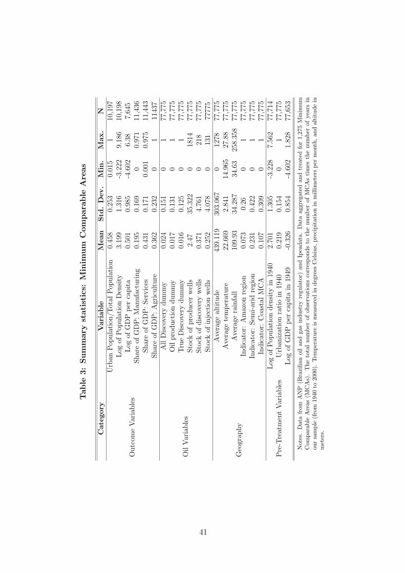
Table

3:Summary

statistics:

Minim

um

Compara

ble

Areas

Category

Variable

Mean

Std

.Dev.

Min.

Max.

N

Outcom

eVariables

Urban

Pop

ulation

/Total

Pop

ulation

0.458

0.253

0.015

110,197

Log

ofPop

ulation

Density

3.199

1.316

-3.222

9.186

10,198

Log

ofGDPper

capita

0.501

0.985

-4.602

6.38

7,645

Shareof

GDP:Man

ufacturing

0.195

0.169

00.971

11,436

Shareof

GDP:Services

0.431

0.171

0.001

0.975

11,443

Shareof

GDP:Agriculture

0.362

0.232

01

11437

OilVariables

AllDiscovery

dummy

0.024

0.151

01

77,775

Oilproductiondummy

0.017

0.131

01

77,775

TrueDiscovery

dummy

0.016

0.125

01

77,775

Stock

ofproducerwells

2.47

35.322

01814

77,775

Stock

ofdiscovery

wells

0.371

4.761

0218

77,775

Stock

ofinjectionwells

0.252

4.078

0131

77775

Geograp

hy

Average

altitude

439.119

303.067

01278

77,775

Average

temperature

22.669

2.841

14.965

27.88

77,775

Average

rainfall

109.93

34.287

34.63

258.358

77,775

Indicator:Amazon

region

0.073

0.26

01

77,775

Indicator:Sem

i-arid

region

0.231

0.422

01

77,775

Indicator:Coastal

MCA

0.107

0.309

01

77,775

Pre-TreatmentVariables

Log

ofPop

ulation

density

in1940

2.701

1.305

-3.228

7.562

77,714

Urban

izationratioin

1940

0.219

0.154

01

77,775

Log

ofGDPper

capitain

1949

-0.326

0.854

-4.602

1.828

77,653

Notes.Datafrom

ANP

(Brazilian

oilan

dgasindustry

regulator)

andIpeadata.

Data

aggregatedan

dtreatedfor1,275

Minim

um

Com

parab

leAreas

(MCAs).Thetotalnumber

ofob

servationscorrespon

dsto

thenumber

ofMCAstimes

thenumber

ofyears

inoursample

(from

1940

to2000).

Tem

perature

ismeasuredin

degrees

Celsius,precipitationin

millimetersper

month,andaltitudein

meters.

41

Table 4: Correlation between Drilling Attempts and Pre-TreatmentCharacteristics

(1) (2) (3) (4) (5) (6) (7) (8)

Dependent variable: Drilling Dummy Drilling Count

Linear LinearLogit Logit

Linear LinearPoisson Poisson

Probability Probability Probability Probability

Urbanization in 1940 0.360*** 0.0575 2.631*** 0.481 82.50*** 28.32 3.682*** 1.284

(0.104) (0.0939) (0.740) (0.837) (27.37) (22.22) (0.679) (0.888)

Pop. Density in 1940 -3.30e-05 -0.000343 -0.000333 -0.00171 1.237 -2.722 0.0418 -0.177

(0.000278) (0.000249) (0.00219) (0.00161) (2.252) (3.354) (0.146) (0.167)

GDP per capita in 1949 -0.0790*** -0.00712 -0.674*** -0.0787 -9.565*** 3.413 -0.534** 0.129

(0.0150) (0.0144) (0.161) (0.156) (3.657) (8.567) (0.212) (0.404)

Semiarid Indicator 0.00742 0.0938 20.63 1.292*

(0.0220) (0.232) (19.95) (0.782)

Amazon Indicator 0.395*** 2.292*** -7.137 -0.809*

(0.0530) (0.276) (7.567) (0.470)

Coastal Indicator 0.518*** 2.776*** 90.65*** 3.001***

(0.0443) (0.243) (34.54) (0.651)

Constant 0.176*** 0.0934*** -1.513*** -2.314*** -9.173 3.725 1.471*** 1.572***

(0.019) (0.018) (0.138) (0.184) (6.994) (8.538) (0.546) (0.374)

Observations 1,275 1,275 1,275 1,275 1,273 1,273 1,273 1,273

R-squared 0.024 0.255 - - 0.008 0.053 - -

Notes. Robust standard errors in parentheses. The regressions are for 1,275 Minimum Comparable Areas (MCAs). There are two dependentvariables: a dummy variable if any drilling attempt happen during 1940 to 2000 (columns (1) to (4) of the table) and the number of drillingattempts during 1940 and 2000 (columns (5) to (9) of the table). Pre-treatment variables are: urbanization rate in 1940, population density in1940 and per capita GDP in 1949. Geographical controls are indicator variables showing whether the MCA is located in the Semiarid region, inthe Amazon region, or on the coast.*** p<0.01, ** p<0.05, * p<0.1

42

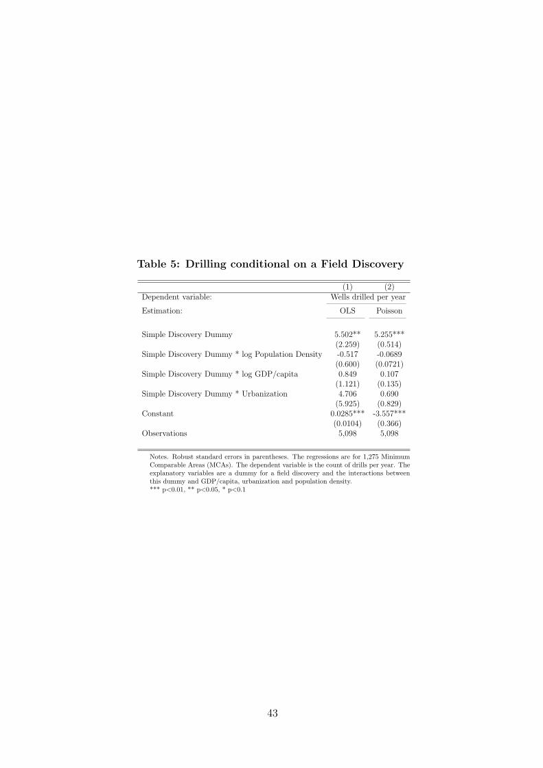
Table 5: Drilling conditional on a Field Discovery

(1) (2)Dependent variable: Wells drilled per year

Estimation: OLS Poisson

Simple Discovery Dummy 5.502** 5.255***(2.259) (0.514)

Simple Discovery Dummy * log Population Density -0.517 -0.0689(0.600) (0.0721)

Simple Discovery Dummy * log GDP/capita 0.849 0.107(1.121) (0.135)

Simple Discovery Dummy * Urbanization 4.706 0.690(5.925) (0.829)

Constant 0.0285*** -3.557***(0.0104) (0.366)

Observations 5,098 5,098

Notes. Robust standard errors in parentheses. The regressions are for 1,275 MinimumComparable Areas (MCAs). The dependent variable is the count of drills per year. Theexplanatory variables are a dummy for a field discovery and the interactions betweenthis dummy and GDP/capita, urbanization and population density.*** p<0.01, ** p<0.05, * p<0.1

43

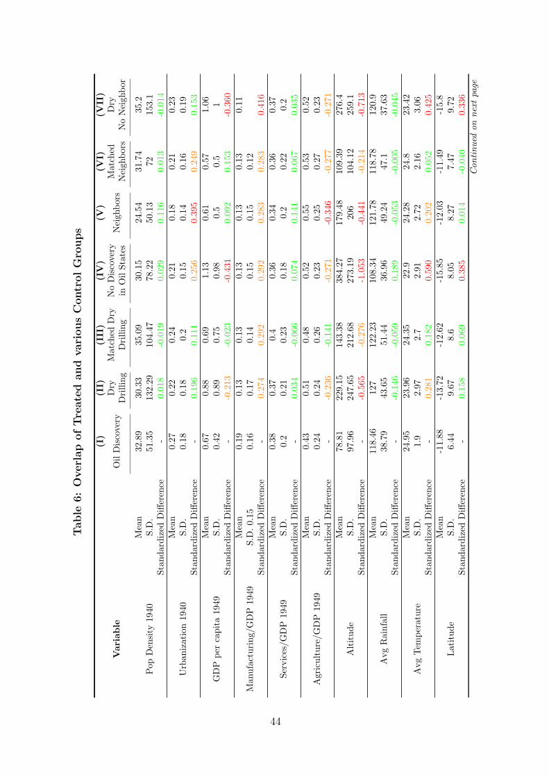
Table

6:OverlapofTreatedand

variousControlGro

ups

(I)

(II)

(III)

(IV)

(V)

(VI)

(VII)

Variable

OilDiscovery

Dry

Matched

Dry

NoDiscovery

Neigh

bors

Matched

Dry

Drilling

Drilling

inOilStates

Neigh

bors

NoNeigh

bor

PopDen

sity

194

0Mean

32.89

30.33

35.09

30.15

24.54

31.74

35.2

S.D

.51

.35

132.29

104.47

78.22

50.13

72153.1

Standardized

Differen

ce-

0.01

8-0.019

0.029

0.116

0.013

-0.014

Urban

ization

194

0Mean

0.27

0.22

0.24

0.21

0.18

0.21

0.23

S.D

.0.18

0.18

0.2

0.15

0.14

0.16

0.19

Standardized

Differen

ce-

0.19

60.11

10.256

0.395

0.249

0.153

GDP

per

capita19

49Mean

0.67

0.88

0.69

1.13

0.61

0.57

1.06

S.D

.0.42

0.89

0.75

0.98

0.5

0.5

1Standardized

Differen

ce-

-0.213

-0.023

-0.431

0.092

0.153

-0.360

Man

ufacturing/

GDP

1949

Mean

0.19

0.13

0.13

0.13

0.13

0.13

0.11

S.D

.0.15

0.16

0.17

0.14

0.15

0.15

0.12

Standardized

Differen

ce-

0.27

40.29

20.292

0.283

0.283

0.416

Services/G

DP

1949

Mean

0.38

0.37

0.4

0.36

0.34

0.36

0.37

S.D

.0.2

0.21

0.23

0.18

0.2

0.22

0.2

Standardized

Differen

ce-

0.03

4-0.066

0.074

0.141

0.067

0.035

Agriculture/G

DP

194

9Mean

0.43

0.51

0.48

0.52

0.55

0.53

0.52

S.D

.0.24

0.24

0.26

0.23

0.25

0.27

0.23

Standardized

Differen

ce-

-0.236

-0.141

-0.271

-0.346

-0.277

-0.271

Altitude

Mean

78.81

229.15

143.38

384

.27

179

.48

109.39

276.4

S.D

.97

.96

247.65

212.68

273.19

206

104.12

259.1

Standardized

Differen

ce-

-0.565

-0.276

-1.053

-0.441

-0.214

-0.713

AvgRainfall

Mean

118.46

127

122.23

108

.34

121

.78

118.78

120.9

S.D

.38

.79

43.65

51.44

36.96

49.24

47.1

37.63

Standardized

Differen

ce-

-0.146

-0.059

0.189

-0.053

-0.005

-0.045

AvgTem

perature

Mean

24.95

23.96

24.35

22.9

24.28

24.8

23.42

S.D

.1.9

2.97

2.7

2.91

2.72

2.16

3.06

Standardized

Differen

ce-

0.28

10.18

20.590

0.202

0.052

0.425

Latitude

Mean

-11.88

-13.72

-12.62

-15.85

-12.03

-11.49

-15.8

S.D

.6.44

9.67

8.6

8.05

8.27

7.47

9.72

Standardized

Differen

ce-

0.15

80.06

90.385

0.014

-0.040

0.336

Continued

onnextpage

44

Tab

le6–Continued

from

previouspage

Variable

OilDiscovery

Dry

Matched

Dry

NoDiscovery

Neighbors

Matched

Dry

Drilling

Drilling

inOilStates

Neigh

bors

NoNeigh

bor

Longitude

Mean

-40.65

-46.94

-43.5

-44.53

-44.32

-42.65

-46.83

S.D

.6.46

7.31

7.6

5.18

8.46

8.33

5.42

Standardized

Differen

ce-

0.64

50.28

60.469

0.345

0.190

0.733

Coa

stal

Indicator

Prop.

0.59

0.3

0.53

0.11

0.19

0.42

0.29

Standardized

Differen

ce-

0.43

10.08

60.823

0.636

0.244

0.448

Sem

iaridIndicator

Prop.

0.19

0.15

0.23

0.25

0.25

0.28

0.13

Standardized

Differen

ce-

0.07

5-0.070

-0.103

-0.103

-0.151

0.116

Amazon

Indicator

Prop.

0.08

0.3

0.17

0.1

0.23

0.15

0.25

Standardized

Differen

ce-

-0.413

-0.194

-0.049

-0.300

-0.156

-0.333

Number

ofMCAs

6415

864

711

156

64104

Note:OilDiscoveryisthetreatedgroupof

64MCAs.

Six

control

grou

psareshow

n:(i)MCAswheredrillingtook

place

butnothingwas

found(columnII:

“Dry

Drilling”),Propen

sity

Score

Matched

Sam

ple

ofMCAswheredrillingtook

place

butnothingwasfound(columnIII:“Matched

Dry

Drilling”),(iii)

MCAswithnooildiscovery

butin

states

whereother

MCAshavediscoveredoil(columnIII:“N

oDiscovery

inOilStates”,(iv)MCAsthat

aread

jacent

tothetreatedMCAs(columnIV

:“N

eighbors”),

(v)Propen

sity

Score

Matched

Sam

ple

ofMCAsthat

are

adjacentto

thetreatedMCAs(columnVI:

“Matched

Neighbors”),an

d(vi)MCAswheredrillingtook

place

butnothingwas

foundwhichare

notad

jacentto

treatedMCAs(columnVII:“D

ry,No

Neigh

bou

r”).

(i)and(ii)

areou

rbaselinecontrol

groups.

Weuse

theother

fourin

arobustnessexercise.Thelast

row

correspon

dsto

thetotalnumber

ofMCAsin

each

controlgrou

p.

45

Table 7: Discovery Dummy: Analysis

Dependent Variable: Oil Production(1) (2)

All Discoveries 0.681***(0.0524)

True Discoveries 0.777***(0.0472)

MCA FE Yes YesYear FE Yes YesObservations 8,901 8,901Number of MCAs 1,273 1,273Geography Controls Yes YesInitial Conditions Yes YesEstimation FE FEF-Statistics 9.86 20.41

Notes. Standard errors clustered at the MCAlevel. Explanatory variables are three dummiesrelated to oil discovery. Geographic controls andinitial conditions have time-varying coefficients.The initial conditions with time-varying coeffi-cients are: GDP/capita in 1949, Urbanizationrate in 1940, and Population Density in 1940.The geographic controls with time-varying coef-ficients are: Latitude and Longitude coordinates,Dummy for Amazon, Dummy for Coastal. Thetotal sample consists of 1,275 Minimum Compa-rable Areas (MCA).*** p<0.01, ** p<0.05, * p<0.1

46

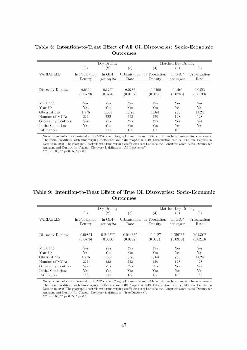
Table 8: Intention-to-Treat Effect of All Oil Discoveries: Socio-EconomicOutcomes

Dry Drilling Matched Dry Drilling(1) (2) (3) (4) (5) (6)

VARIABLES ln Population ln GDP Urbanization ln Population ln GDP UrbanizationDensity per capita Rate Density per capita Rate

Discovery Dummy -0.0390 0.125* 0.0283 -0.0400 0.146* 0.0253(0.0579) (0.0728) (0.0187) (0.0626) (0.0783) (0.0199)

MCA FE Yes Yes Yes Yes Yes YesYear FE Yes Yes Yes Yes Yes YesObservations 1,776 1,332 1,776 1,024 768 1,024Number of MCAs 222 222 222 128 128 128Geography Controls Yes Yes Yes Yes Yes YesInitial Conditions Yes Yes Yes Yes Yes YesEstimation FE FE FE FE FE FE

Notes. Standard errors clustered at the MCA level. Geographic controls and initial conditions have time-varying coefficients.The initial conditions with time-varying coefficients are: GDP/capita in 1949, Urbanization rate in 1940, and PopulationDensity in 1940. The geographic controls with time-varying coefficients are: Latitude and Longitude coordinates, Dummy forAmazon, and Dummy for Coastal. Discovery is defined as “All Discoveries”.*** p<0.01, ** p<0.05, * p<0.1

Table 9: Intention-to-Treat Effect of True Oil Discoveries: Socio-EconomicOutcomes

Dry Drilling Matched Dry Drilling(1) (2) (3) (4) (5) (6)

VARIABLES ln Population ln GDP Urbanization ln Population ln GDP UrbanizationDensity per capita Rate Density per capita Rate

Discovery Dummy -0.00864 0.246*** 0.0443** -0.0127 0.259*** 0.0430**(0.0676) (0.0856) (0.0202) (0.0731) (0.0910) (0.0213)

MCA FE Yes Yes Yes Yes Yes YesYear FE Yes Yes Yes Yes Yes YesObservations 1,776 1,332 1,776 1,024 768 1,024Number of MCAs 222 222 222 128 128 128Geography Controls Yes Yes Yes Yes Yes YesInitial Conditions Yes Yes Yes Yes Yes YesEstimation FE FE FE FE FE FE

Notes. Standard errors clustered at the MCA level. Geographic controls and initial conditions have time-varying coefficients.The initial conditions with time-varying coefficients are: GDP/capita in 1949, Urbanization rate in 1940, and PopulationDensity in 1940. The geographic controls with time-varying coefficients are: Latitude and Longitude coordinates, Dummy forAmazon, and Dummy for Coastal. Discovery is defined as “True Discovery”.*** p<0.01, ** p<0.05, * p<0.1

47

Table 10: Intention-to-Treat Effect of Oil Discoveries: Robustness toalternative control groups

Non-Oil Municipalities in Oil States Dry Drilling, No Neighbors(1) (2) (3) (4) (5) (6)

VARIABLES ln Population ln GDP Urbanization ln Population ln GDP UrbanizationDensity per capita Rate Density per capita Rate

Discovery Dummy -0.0560 0.262*** 0.0519*** -0.0302 0.195** 0.0362*(0.0610) (0.0781) (0.0190) (0.0751) (0.0906) (0.0214)

MCA FE Yes Yes Yes Yes Yes YesYear FE Yes Yes Yes Yes Yes YesObservations 6,200 4,649 6,200 1,344 1,008 1,344Number of MCAs 775 775 775 168 168 168Geography Controls Yes Yes Yes Yes Yes YesInitial Conditions Yes Yes Yes Yes Yes YesEstimation FE FE FE FE FE FE

All Neighbors Matched Neighbors(1) (2) (3) (4) (5) (6)

VARIABLES ln Population ln GDP Urbanization ln Population ln GDP UrbanizationDensity per capita Rate Density per capita Rate

Discovery Dummy 0.0114 0.247*** 0.0434** 0.0341 0.277*** 0.0419**(0.0641) (0.0819) (0.0195) (0.0645) (0.0863) (0.0206)

MCA FE Yes Yes Yes Yes Yes YesYear FE Yes Yes Yes Yes Yes YesObservations 1,760 1,320 1,760 1,024 768 1,024Number of MCAs 220 220 220 128 128 128Geography Controls Yes Yes Yes Yes Yes YesInitial Conditions Yes Yes Yes Yes Yes YesEstimation FE FE FE FE FE FE

Notes. Standard errors clustered at the MCA level. Geographic controls and initial conditions have time-varying coefficients.The initial conditions with time-varying coefficients are: GDP/capita in 1949, Urbanization rate in 1940, and PopulationDensity in 1940. The geographic controls with time-varying coefficients are: Latitude and Longitude coordinates, Dummy forAmazon, and Dummy for Coastal. Discovery is defined as “True Discovery”.*** p<0.01, ** p<0.05, * p<0.1

48

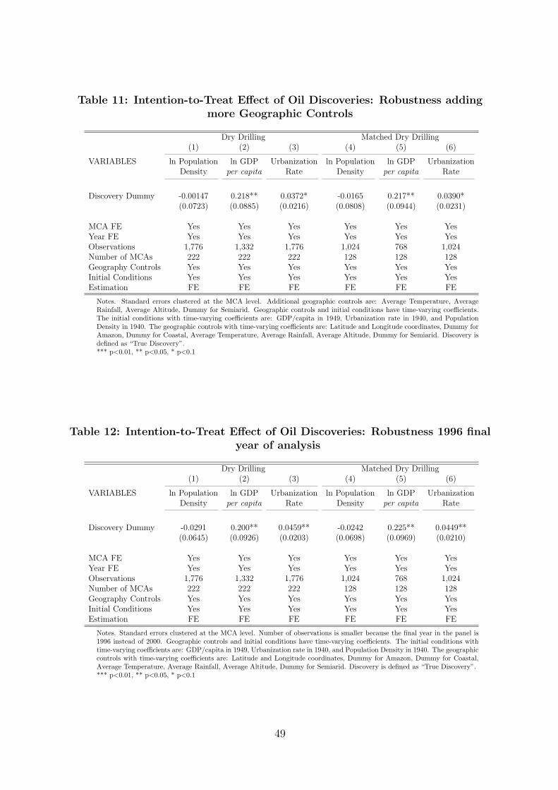
Table 11: Intention-to-Treat Effect of Oil Discoveries: Robustness addingmore Geographic Controls

Dry Drilling Matched Dry Drilling(1) (2) (3) (4) (5) (6)

VARIABLES ln Population ln GDP Urbanization ln Population ln GDP UrbanizationDensity per capita Rate Density per capita Rate

Discovery Dummy -0.00147 0.218** 0.0372* -0.0165 0.217** 0.0390*(0.0723) (0.0885) (0.0216) (0.0808) (0.0944) (0.0231)

MCA FE Yes Yes Yes Yes Yes YesYear FE Yes Yes Yes Yes Yes YesObservations 1,776 1,332 1,776 1,024 768 1,024Number of MCAs 222 222 222 128 128 128Geography Controls Yes Yes Yes Yes Yes YesInitial Conditions Yes Yes Yes Yes Yes YesEstimation FE FE FE FE FE FE

Notes. Standard errors clustered at the MCA level. Additional geographic controls are: Average Temperature, AverageRainfall, Average Altitude, Dummy for Semiarid. Geographic controls and initial conditions have time-varying coefficients.The initial conditions with time-varying coefficients are: GDP/capita in 1949, Urbanization rate in 1940, and PopulationDensity in 1940. The geographic controls with time-varying coefficients are: Latitude and Longitude coordinates, Dummy forAmazon, Dummy for Coastal, Average Temperature, Average Rainfall, Average Altitude, Dummy for Semiarid. Discovery isdefined as “True Discovery”.*** p<0.01, ** p<0.05, * p<0.1

Table 12: Intention-to-Treat Effect of Oil Discoveries: Robustness 1996 finalyear of analysis

Dry Drilling Matched Dry Drilling(1) (2) (3) (4) (5) (6)

VARIABLES ln Population ln GDP Urbanization ln Population ln GDP UrbanizationDensity per capita Rate Density per capita Rate

Discovery Dummy -0.0291 0.200** 0.0459** -0.0242 0.225** 0.0449**(0.0645) (0.0926) (0.0203) (0.0698) (0.0969) (0.0210)

MCA FE Yes Yes Yes Yes Yes YesYear FE Yes Yes Yes Yes Yes YesObservations 1,776 1,332 1,776 1,024 768 1,024Number of MCAs 222 222 222 128 128 128Geography Controls Yes Yes Yes Yes Yes YesInitial Conditions Yes Yes Yes Yes Yes YesEstimation FE FE FE FE FE FE

Notes. Standard errors clustered at the MCA level. Number of observations is smaller because the final year in the panel is1996 instead of 2000. Geographic controls and initial conditions have time-varying coefficients. The initial conditions withtime-varying coefficients are: GDP/capita in 1949, Urbanization rate in 1940, and Population Density in 1940. The geographiccontrols with time-varying coefficients are: Latitude and Longitude coordinates, Dummy for Amazon, Dummy for Coastal,Average Temperature, Average Rainfall, Average Altitude, Dummy for Semiarid. Discovery is defined as “True Discovery”.*** p<0.01, ** p<0.05, * p<0.1

49

Table 13: Intention-to-Treat Effect of Oil Discoveries: Sectoral GDP percapita

Dry Drilling Matched Dry Drilling(1) (2) (3) (4) (5) (6)

VARIABLES Manufacturing Service Agriculture Manufacturing Service AgricultureGDP per cap GDP per cap GDP per cap GDP per cap GDP per cap GDP per cap

Discovery Dummy 0.449** 0.213** 0.0569 0.456** 0.215** 0.0664(0.182) (0.0968) (0.107) (0.189) (0.104) (0.109)

MCA FE Yes Yes Yes Yes Yes YesYear FE Yes Yes Yes Yes Yes YesObservations 1,325 1,321 1,328 765 764 765Number of MCAs 222 222 222 128 128 128Geography Controls Yes Yes Yes Yes Yes YesInitial Conditions Yes Yes Yes Yes Yes YesEstimation FE FE FE FE FE FE

Notes. Standard errors clustered at the MCA level. Geographic controls and initial conditions have time-varying coefficients. Theinitial conditions with time-varying coefficients are: GDP/capita in 1949, Urbanization rate in 1940, and Population Density in 1940.The geographic controls with time-varying coefficients are: Latitude and Longitude coordinates, Dummy for Amazon, and Dummy forCoastal. Discovery is defined as “True Discovery”.*** p<0.01, ** p<0.05, * p<0.1

Table 14: Intention-to-Treat Effect of Oil Discoveries: Sectoral LaborProductivity per capita

Dry Drilling Matched Dry Drilling(1) (2) (3) (4) (5) (6)

VARIABLES Manufacturing Service Agriculture Manufacturing Service AgricultureLabor Prod. Labor Prod. Labor Prod. Labor Prod. Labor Prod. Labor Prod.

Discovery Dummy 0.265* 0.221** -0.0717 0.222 0.188* -0.0535(0.139) (0.106) (0.0881) (0.143) (0.113) (0.0871)

MCA FE Yes Yes Yes Yes Yes YesYear FE Yes Yes Yes Yes Yes YesObservations 1,533 1,542 1,547 883 891 891Number of MCAs 222 222 222 128 128 128Geography Controls Yes Yes Yes Yes Yes YesInitial Conditions Yes Yes Yes Yes Yes YesEstimation FE FE FE FE FE FE

Notes. Standard errors clustered at the MCA level. Geographic controls and initial conditions have time-varying coefficients. Theinitial conditions with time-varying coefficients are: GDP/capita in 1949, Urbanization rate in 1940, and Population Density in1940. The geographic controls with time-varying coefficients are: Latitude and Longitude coordinates, Dummy for Amazon, andDummy for Coastal. Discovery is defined as “True Discovery”.*** p<0.01, ** p<0.05, * p<0.1

50

Table 15: Onshore versus Offshore Discoveries 1

Matched Dry Drilling(1) (2) (3) (4)

VARIABLES GDP Manufacturing GDP GDP Manufacturing GDPper cap per cap per cap per cap

Onshore Discovery Dummy 0.3429*** 0.5270**(0.1067) (0.2157)

Offshore Discovery Dummy 0.2081 0.4537*(0.1315) (0.2303)

MCA FE Yes Yes Yes YesYear FE Yes Yes Yes YesObservations 768 891 768 891Number of MCAs 128 128 128 128Geography Controls Yes Yes Yes YesInitial Conditions Yes Yes Yes YesEstimation FE FE FE FE

Notes. Standard errors clustered at the MCA level. The main explanatory variable is the number of injectionwells. The number of injection and production wells is instrumented with the number of discovery wells. Geo-graphic controls and initial conditions have time-varying coefficients. The initial conditions with time-varyingcoefficients are: GDP/capita in 1949, Urbanization rate in 1940, and Population Density in 1940. The geographiccontrols with time-varying coefficients are: Latitude and Longitude coordinates, Dummy for Amazon, Dummyfor Coastal. The control group is the matched dry drilling sample.*** p<0.01, ** p<0.05, * p<0.1

Table 16: Onshore versus Offshore Discoveries 2

Matched Dry Drilling(1) (2) (3) (4)

VARIABLES Service Urbanization Service UrbanizationLabor Prod. Rate Labor Prod. Rate

Onshore Discovery Dummy 0.280** 0.0542**(0.135) (0.0237)

Offshore Discovery Dummy 0.0187 0.0135(0.126) (0.0313)

MCA FE Yes Yes Yes YesYear FE Yes Yes Yes YesObservations 891 1,024 891 1,024Number of MCAs 128 128 128 128Geography Controls Yes Yes Yes YesInitial Conditions Yes Yes Yes YesEstimation FE FE FE FE

Notes. Standard errors clustered at the MCA level. The main explanatory variable is the numberof injection wells. The number of injection and production wells is instrumented with the number ofdiscovery wells. Geographic controls and initial conditions have time-varying coefficients. The initialconditions with time-varying coefficients are: GDP/capita in 1949, Urbanization rate in 1940, andPopulation Density in 1940. The geographic controls with time-varying coefficients are: Latitude andLongitude coordinates, Dummy for Amazon, Dummy for Coastal. The control group is the matcheddry drilling sample.*** p<0.01, ** p<0.05, * p<0.1

51

Table 17: Local Average Treatment Effect of Oil Production

Matched Dry Drilling(1) (2) (3) (4) (5) (6)

VARIABLES ln Population ln GDP Urbanization Manufacturing Service AgricultureDensity per capita Rate GDP per cap GDP per cap GDP per cap

Production Dummy -0.0190 0.411*** 0.0644** 0.725** 0.343** 0.105(0.106) (0.143) (0.0314) (0.295) (0.166) (0.166)

First Stage F-Stat. 27.38 13.74 27.38 13.33 14.48 13.89MCA FE Yes Yes Yes Yes Yes YesYear FE Yes Yes Yes Yes Yes YesObservations 1,024 768 1,024 765 764 765Number of MCAs 128 128 128 128 128 128Geography Controls Yes Yes Yes Yes Yes YesInitial Conditions Yes Yes Yes Yes Yes YesEstimation FE FE FE FE FE FE

Notes. Standard errors clustered at the MCA level. Geographic controls and initial conditions have time-varying coefficients. Theinitial conditions with time-varying coefficients are: GDP/capita in 1949, Urbanization rate in 1940, and Population Density in1940. The geographic controls with time-varying coefficients are: Latitude and Longitude coordinates, Dummy for Amazon, andDummy for Coastal. Production is instrumented with Discovery. Discovery is defined as ’True Discovery’.*** p<0.01, ** p<0.05, * p<0.1

Table 18: Treatment Intensity

Matched Dry Drilling(1) (2) (3) (4)

VARIABLES ln GDP Urbanization ln GDP Urbanizationper capita Rate per capita Rate

Number of Production Wells 0.000664** 7.55e-05**(0.000317) (3.70e-05)

Number of Injection Wells 0.0123** 0.00146*(0.00573) (0.000871)

First Stage F-Stat. 6.98 15.92 6.29 31.21MCA FE Yes Yes Yes YesYear FE Yes Yes Yes YesObservations 768 1,024 768 1,024Number of MCAs 128 128 128 128Geography Controls Yes Yes Yes YesInitial Conditions Yes Yes Yes YesEstimation FE FE FE FE

Notes. Standard errors clustered at the MCA level. The main explanatory variable is the number of injectionwells. The number of injection and production wells is instrumented with the number of discovery wells.Geographic controls and initial conditions have time-varying coefficients. The initial conditions with time-varying coefficients are: GDP/capita in 1949, Urbanization rate in 1940, and Population Density in 1940.The geographic controls with time-varying coefficients are: Latitude and Longitude coordinates, Dummy forAmazon, Dummy for Coastal. The number of discovery wells is used an as instrument.*** p<0.01, ** p<0.05, * p<0.1

52

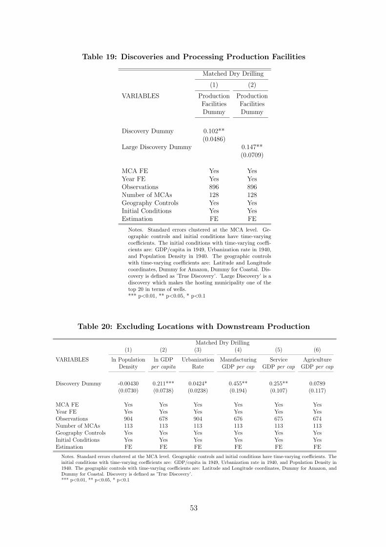
Table 19: Discoveries and Processing Production Facilities

Matched Dry Drilling

(1) (2)

VARIABLES Production ProductionFacilities FacilitiesDummy Dummy

Discovery Dummy 0.102**(0.0486)

Large Discovery Dummy 0.147**(0.0709)

MCA FE Yes YesYear FE Yes YesObservations 896 896Number of MCAs 128 128Geography Controls Yes YesInitial Conditions Yes YesEstimation FE FE

Notes. Standard errors clustered at the MCA level. Ge-ographic controls and initial conditions have time-varyingcoefficients. The initial conditions with time-varying coeffi-cients are: GDP/capita in 1949, Urbanization rate in 1940,and Population Density in 1940. The geographic controlswith time-varying coefficients are: Latitude and Longitudecoordinates, Dummy for Amazon, Dummy for Coastal. Dis-covery is defined as ’True Discovery’. ’Large Discovery’ is adiscovery which makes the hosting municipality one of thetop 20 in terms of wells.*** p<0.01, ** p<0.05, * p<0.1

Table 20: Excluding Locations with Downstream Production

Matched Dry Drilling(1) (2) (3) (4) (5) (6)

VARIABLES ln Population ln GDP Urbanization Manufacturing Service AgricultureDensity per capita Rate GDP per cap GDP per cap GDP per cap

Discovery Dummy -0.00430 0.211*** 0.0424* 0.455** 0.255** 0.0789(0.0730) (0.0738) (0.0238) (0.194) (0.107) (0.117)

MCA FE Yes Yes Yes Yes Yes YesYear FE Yes Yes Yes Yes Yes YesObservations 904 678 904 676 675 674Number of MCAs 113 113 113 113 113 113Geography Controls Yes Yes Yes Yes Yes YesInitial Conditions Yes Yes Yes Yes Yes YesEstimation FE FE FE FE FE FE

Notes. Standard errors clustered at the MCA level. Geographic controls and initial conditions have time-varying coefficients. Theinitial conditions with time-varying coefficients are: GDP/capita in 1949, Urbanization rate in 1940, and Population Density in1940. The geographic controls with time-varying coefficients are: Latitude and Longitude coordinates, Dummy for Amazon, andDummy for Coastal. Discovery is defined as ’True Discovery’.*** p<0.01, ** p<0.05, * p<0.1

53

B Appendix: On Drilling and Production

There is an extensive literature on the principles and practises of oil drilling and production(e.g., from petroleum geology and petroleum engineering). In this appendix, we aim toclarify selected aspects of drilling and production that are relevant to our research design,without detailing every single aspect of oil (and gas) exploration and production.

Oil exploration and production are associated with risk. Although there are severaltechnical methods for appraising hydrocarbon resources, the industry always works withlimited information on the existence of hydrocarbon deposits. The uncertainty is relatedto the location, volume, and quality of hydrocarbon deposits. Even with enough geologicalinformation, there is always the risk of drilling a dry exploratory hole or not discoveringcommercial quantities of oil. There are also risks during the production phase such as theprice of oil, costs and taxes, institutional uncertainty, regulation, natural disasters, andaccidents. Offshore drilling in deep water presents even greater challenges. According toHarbaugh, Davis, and Wendebourg (1995), luck is a major factor in oil exploration. Thename for an exploratory well (called a “wildcat”) talks by itself regarding the inherent riskof oil business.

The petroleum industry is loosely divided into two segments: upstream and down-stream. Upstream industry comprises exploration and production activities. By produc-tion activities, the process of recovering petroleum from the subsurface is meant. Upstreamactivities occur both onshore and offshore. In turn, downstream industry entails process-ing, retailing and transporting petroleum.

Oil exploration involves several steps using a compilation of knowledge from geology,geophysics, and geochemistry. The oil company aims to find an oil field - a contiguousgeographic area with oil. First, petroleum professionals collect useful geological informa-tion on a “prospect” (a delimited area that possesses certain geological features that mayinduce drilling). By “useful information”, they mean a source rock, a reservoir, and atrap42. A source rock is a rock within which oil or gas is generated from organic material(Petroleum Extension Service (2005)). A source rock is usually a shale rock. Nevertheless,not every shale has enough biogenic material to be classified as a source rock. The reservoiraccumulates hydrocarbons and is made from porous rocks. Rocks must have porosity toaccumulate hydrocarbons and basically only sedimentary rocks are porous enough. Typi-cal sedimentary rocks forming a reservoir include sandstone and limestone. The “quality”of the oil inside the reservoir can vary depending on its properties and impurities (e.g., thepresence of sulfur and metals). The company also looks for areas with specific geologicalfeatures called traps. The hydrocarbon trap is composed of two elements: a structure(subsurface contortion) and a seal. Hydrocarbon molecules are lighter than water, andthere are subsurface contortions that induce the hydrocarbons moving upward towards thesurface (e.g., anticlines and faults). Therefore, there is a need of a “seal” to prevent thehydrocarbons from spilling out on the surface. A seal is another rock with low perme-ability (as porosity to accumulate hydrocarbons in the reservoir is important, the degreeof connections between pore spaces of the rock formation is relevant to have a seal rock).Shale rock is typically a good seal to avoid the spilling because it has low permeability.

42There are three type of rocks according to how they are formed: ignite (from magma), sedimentary(from erosion) and metamorphic (a heated sedimentary or a heated ignite rock). Sedimentary rocks aremore interesting because petroleum accumulation chiefly occur in them. An example of a sedimentaryrock is the shale rock, originated by clay compacted by subsurface pressure and weight. Other examplesof sedimentary rocks include sandstone (from sand) and limestone (from shells).

54

Shale rock has porosity too, but it has very low permeability (thus it is a good seal).In sum, the area should contain selected characteristics, such as abundant sandstone

reservoir rocks, shale for hydrocarbon source rock and numerous geological structures forpotential trapping of hydrocarbons. Each oil field has a “fingerprint” and its uniquecharacteristics lead to a case-by-case analysis of drilling attempts. Wells are very expensiveto drill, so previous studies must be as accurate and precise as possible.

After inferring the subsurface and if there are strong indications of potentially oil-bearing formations, the oil company may drill an exploratory well. Even with all positiveindications of oil presence, only by making a hole can the company be sure of the pres-ence (or absence) of oil. During the drilling process, data acquisition is key. There areseveral logging (recording information) procedures during the drilling phase so as to, forexample, differentiate permeable and impermeable rock formations (called “‘logging-while-drilling”).43 Depending on the outcome of the exploratory drilling, the company evaluatesthe well’s hydrocarbon potential. Not even an evidence of hydrocarbon deposit as told bylogs is a guarantee that producing oil is really possible. One can assign a priori probabilitiesbefore drilling, and revise the probability of success given the proven result of the drillingattempt. Updated probabilities can be used as a source of experience to be transferredto future drilling attempts. Depending on the preliminary information received duringdrilling, the well can be abandoned or not. In the end, using all information available thecompany decides whether the drilling had generated a discovery or a dry hole.

After a discovery, the appraisal continues: additional drilling is required to delineate thesize and extension of the oil field44. “Step-out” wells (delineation or appraising wells) arethe wells used to evaluate the extent of the field. The more is known about the oil field, theeasier and less expensive to drill additional wells. Generally, the number of step-out wellsis positively correlated with the magnitude of the field that was discovered. Once the oilcompany has delineated the oil field and is secure on the viability of production, it starts to(i) complete the existing wells and (ii) to drill additional production wells (producer wells).To complete a well means to perform the necessary operations to bring fluids to the surface(Petroleum Extension Service (1997)). After completion and the drilling of producer wells,oil and gas production cycle begins. Production cycle occurs after exploration has provensuccessful. An economic assessment of the production cycle should entail reserve and riskcalculations (Hyne (2001)).

The production cycle involves a natural phase and enhanced phase. Initially, naturalpressure from the reservoir brings oil from the reservoir to the surface. As productionproceeds, the reservoir pressure goes down. However, pressure is important because itdrives oil and gas out of the reservoir. Normally, after some time producing from an oilwell, pressure decreases and the oil company needs to (artificially) add pressure to the well.The addition of artificial pressure to optimize production is broadly called “enhanced oilrecovery” and is divided into primary, secondary, and tertiary recovery. Primary recovery(or primary production) means to use an artificial method of lifting. The most commonartificial lift system is a beam pump to pump up the oil. During primary recovery, onlya small percentage of the hydrocarbon deposits are produced. Secondary recovery aimsat restoring the reservoir pressure by injecting water (waterflooding) or gas. Secondaryrecovery is costly because it deals with huge amounts of water and gas. To supplementfalling pressure due to production, new wells are drilled (injection wells) to inject water

43One example is the logging from the drilling fluid.44“Play” is the name used to describe the extent of a hydrocarbon-bearing formation.

55

and gas usually at the edges of the oil field. This injection aims to either slow productiondecline or to increase production. Finally, tertiary recovery happens when there is injectionof steam or special chemicals (chemical flooding) into the reservoir. In practise, all threerecovery phases can occur concomitantly45.

Enhanced recovery is so important in the petroleum industry that the location of theproducer well is chosen with the secondary well (injection well) in mind. As mentionedbefore, efforts to enhance recovery are costly and are dependent upon the state of the econ-omy and potential oil recovery volume. Consequently, repeated monitoring of a reservoir isessential to locate injection wells. The idea is to design an optimal distribution of injectionwells to optimize long-term production.

There are several types of wells: wildcat well, rank wildcat well, step-out well, producerwell, injection well, etc. Since there are different steps to obtain oil, wells are classifiedbroadly as exploratory wells and development wells. Examples of exploratory wells arewildcat wells (drilled a mile or more from an area of existing oil production) and rankwildcat wells (drilled in an area where there is no existing production). If the exploratorydrilling is proven successful, the company starts to drill step-out wells (also included inthe exploratory well category). After the oil field has been delineated, the company startsto drill production wells in the known extent of the field. Every well drilled inside theknown extent of the field is called development wells (Hyne (2001)). The developmentwell category includes producer wells and injection wells (recall that injection wells are toenhance oil recovery). Different categories of wells have different probabilities of finding oil.A rank wildcat exploratory well have on average lower success ratio than a step-out well.An oil company can rank wells in terms of probability even working under uncertainty.The American Petroleum Institute reported that in 2000 the success rate for wildcat wellwas 39% (Hyne (2001)). Note that an unsuccessful drilling is classified as a dry hole inboth exploratory and development well categories.

The evolution of knowledge to identify potentially oil-bearing formations also helpsto understand the oil industry. This evolution comprises both advances of the theory onpetroleum-bearing formations and ever-improving technology. In the very beginning of oilexploration, conspicuous targets were searched in order to extract oil without any geologytheory (e.g., surface pools in the form of natural oil seeps) or using geology knowledge (e.g.,anticlines and salt domes). Surface investigation (topography) of the region could pointout conspicuous areas of oil-bering formations. In 1920’s and 1930’s, aerial photographicexpanded the possibilities for mapping areas suitable for drilling. In the mid 1900’s, seismictechnology improved subsurface mapping to locate potential petroleum-bearing formations.By and large, seismic activities produce sound waves that aim at interpreting subsurfaceformations, i.e., sound waves are generated and recorded by receivers to infer rock forma-tions. The idea is to map the subsurface rock layers by using sound waves as differentrock layers have different acoustical properties. The recorded sounds are processed andassembled to be interpreted. Existing seismic and well information highlights the potentialfor exploration of large hydrocarbon resources. Computerization of seismic data provideda leap to the extraction industry: high amount of data could be processed at high speedand precision. Another big revolution was the 3D visualization that made possible a morereliable selection of the best targets to the drilled. Moreover, 4D visualization (repeated3D through time) helped the planning of well life-time operation. More recently, in thelast decade the discussion on automated drilling (the evolution of automation in drilling)

45There are other forms of well stimulation such as hydraulic fracturing.

56

is an ongoing topic. Modern technology helps the decisions regarding the best drill sites.Computers and satellite images improved the assessment of deposits. Nevertheless, ulti-mately it is only by drilling that a company can be certain that hydrocarbon depositsreally exist. In other words, even investing substantially in using modern technology, it isonly by drilling that the existence of oil can be confirmed.

Up to this point, we described some general aspects of the upstream industry. Down-stream industry includes the refining industry, petrochemicals plant, and distribution fa-cilities (e.g., ports and terminals). Crude oil and natural gas are of little use in their rawstate (Petroleum Extension Service (1997)). Refining and processing to select groups ofcomponents (called “fractions”) is what creates value. Refining means applying chemi-cal processes to convert fractions into commercial products. Oil and gas vary in theirhydrocarbon compounds and impurities (such as sulfur and metals). For instance, thereare light crude oils as well as heavy and thick crude oils. The complexity of the com-position of petroleum fractions leads to more than 2,000 individual refinery products(Fahim, Al-Sahhaf, and Elkilani (2009)). Examples of refining products include gasoline,jet fuel, kerosene, diesel fuel, and feedstocks for the petrochemical industry.

C Appendix: Royalties and Oil in Brazil

The distribution of Royalties started in 1953. Federal Law n. 2,004/53 stipulated that5% of the revenue from onshore oil production should be distributed to states (80%) andmunicipalities (20%) in the form of Royalties. Offshore oil royalties paid to states andmunicipalities were introduced by 1986. In 1997, Federal Law n. 9,496/97 changed theformula to distribute Royalties (e.g., the international price of oil started to be used inthe distribution formula). This led to a huge increase in royalty payments as illustratedbelow in Figure 10, transforming it from a minor to a very significant source of income formunicipalities.

Fig. 10: Distribution of Royalties: 1994-2000

1994 1995 1996 1997 1998 1999 20000

0.2

0.4

0.6

0.8

1

1.2

1.4

1.6

1.8

2x 10

6

Year

Roy

altie

s (in

thou

sand

s R

$)

Federal + States + MunicipalitiesMunicipalities only

Federal Lawn. 9,496/97

Notes. In 1997, Federal Law n. 9,496/97 changed the rules for distributing royalties.

The rules following the 1997 law require that an oil company must allocate between 5%and 10% of the value of the gross output in the form of royalties. Royalties are then divided

57

among the three administrative levels in Brazil (National, States, and Municipalities).Municipalities are eligible to receive royalties based on (i) geography (if the productiontakes place in their territory or, in the case of offshore production, if it is a “facing”municipality, i.e., there is an oilfield that lies inside the municipality’s maritime border), (ii)oil-related infrastructure (if within their borders there is storage, transportation, or landingof oil and gas), and (iii) an equalization rule (there is a “special fund” that allocates partof the royalties’ revenue to all Brazilian municipalities). For some municipalities, royaltiesrepresent a significant part of their total revenue (more than half of total revenue in extremecases). According to ANP (Brazil’s oil and gas industry regulator), over R$ 4.5 billions(circa US$ 2.2 billion) in oil windfalls were distributed to the Brazilian municipalities in2010, which represented on average 2.5% of the total revenue of municipalities receivingoil windfalls.

For a much more detailed description of the history and technicalities of royalty pay-ments in Brazil see Caselli and Michaels (2013) and Monteiro and Ferraz (2012).

58