calsimetaw and weap models for water...

111

ICID 21st Congress, Tehran, October 2011 Symp.09

CALSIMETAW AND WEAP MODELS FOR WATER DEMAND PLANNING

MODELES CALSIMETAW ET WEAP POUR LA PLANIFICATION DES BESOINS EN EAU

Mohammad Rayej1, Richard. L. Snyder2, Morteza N. Orang3, Shu Geng4 and Sara Sarreshteh5

ABSTRACT

The CALSIMETAW computer model estimates crop evapotranspiration (ETc) and evapotranspiration from applied water (ETaw) for use in California water resources planning. The model accounts for soils, crop coefficients, rooting depths, seepage, etc., that influence crop water balance. It provides spatial soil and climate information and it uses historical crop category information to provide seasonal water balance estimates by combinations of county and detailed analysis units (DAU/County). The seasonal water balance is used to estimate the ETaw by crop category for each DAU/County combination over the State. The model uses monthly PRISM (USDA-NRCS) data or a weather generator to estimate daily maximum and minimum air temperatures and rainfall from monthly means. Reference evapotranspiration (ETo) is estimated from a calibrated Hargreaves-Samani equation that accounts for spatial climate differences. In addition to using historical data, CALSIMETAW can use near-real-time data from the combination of weather station and remote sensing data to provide current ETc and ETaw estimates. The ability to use forecast weather data from the National Weather Service is currently under investigation. Using the weather generator, CALSIMETAW projects possible impacts of climate change on water demand.

As a part of the recent California Water Plan Update (2009), a physically-based water resources model called Water Evaluation and Planning (WEAP) was used to project the impacts of climate change on Agricultural and Urban water demand into the mid-century (2050) planning horizon for the 10 hydrologic regions of California. WEAP is a demand-driven water resources allocation model that integrates sources of supply and demand. It has a powerful scenario-building capability and can be used as a long-term planning tool for water

1 Senior Water Resources Engineer, California Department of Water Resources, 901 P street, 2nd floor, Sacramento, CA, U.S.A. 95814, E-mail: [email protected]

2 Biometeorology Specialist, Univ. of Calif., Dept. of Land, Air and Water Res., Davis, CA 95616, E-mail: [email protected] Senior Land & Water Use Scientist, Calif. Dept. of Water Res., P.O. Box 942836, Sacramento, CA 94236-0001, E-mail: [email protected] Professor,Plant Science (Ret.). Univ. of Calif., Dept. of Land, Air and Water Res., Davis, CA 956165 Junior Specialist, Univ. of Calif., Dept. of Land, Air and Water Res., Davis, CA 95616

ICID 21st International Congress on Irrigation and Drainage, 15-23 October 2011, Tehran, Iran

ICID 21st Congress, Tehran, October 2011 International Commission on Irrigation and Drainage

112

managers and government agencies to explore water management strategies like demand reductions and/or supply augmentations. Similar to CALSIMETAW it uses weather, crop and soil information to estimate ETaw under different climate change scenarios, but on a large scale. There exists, however, a great potential to link CALSIMETAW and WEAP for a more detailed representation of ETaw in space and time in the future.

Key words: Water demand planning, CALSIMETAW and WEAP models, Water balance calculations.

RESUME

Le modèle informatique CALSIMETAW évalue l’évapotranspiration des cultures (ET) et l’évapotranspiration de l’eau appliquée (ETaw) pour une utilisation en planification des ressources hydriques en Californie. Le modèle tient compte des sols, les coefficients des cultures, des profondeurs d’enracinement, d’infiltration, etc. qui influencent l’équilibre de l’eau de la culture. Il fournit les informations du sol et du climatique particulières à un endroit et il utilise les données historiques sur la catégorie des cultures pour fournir une estimation des bilans hydriques saisonniers par des combinaisons de comté et des unités d’analyse détaillée (DAU / Comté). Le bilan hydrique saisonnier est utilisé pour estimer le ETaw selon la catégorie de culture pour chaque combinaison DAU / Comté dans l’Etat. Le modèle utilise les données mensuelles fournies par PRISM (USDA-NRCS) ou un générateur météorologique pour estimer les températures quotidiennes minimales et maximales de l’air et des précipitations selon des moyennes mensuelles. L’évapotranspiration de référence (ETo) est estimée à partir d’une équation calibrée Hargreaves-Samani qui tient compte des différences climatiques particulières à un endroit. A part ces données historiques, CALSIMETAW peut utiliser les données quasi-temps réel par la combinaison de la station météo et des données de télédétection pour fournir un ETc actuel et les estimations d’ETaw. La possibilité d’utiliser les données de prévisions météorologiques du Service météorologique national actuellement fait objet d’enquête. En utilisant le générateur de météo, CALSIMETAW prévoit les impacts possibles du changement climatique sur la demande d’eau.

Dans le cadre de la mise à jour récente de Planification d’eau en Californie (2009), un modèle des ressources en eau d’une base physique appelé l’Evaluation et la Planification d’eau (WEAP) a été mise en œuvre. Ce modèle a été utilisé pour prévenir les impacts du changement climatique sur la demande en eau des secteurs agricoles et urbains dans l’horizon de planification du milieu du siècle (2050) pour les 10 régions hydrologiques de la Californie. WEAP est un modèle d’allocation des ressources en eau et il est axé sur la demande d’eau. Donc il s’agit à la fois des sources d’approvisionnement et de la demande. Il a une puissante capacité de la construction de scénarios et peut être utilisé comme un outil de planification à long terme pour les gestionnaires de l’eau et les organismes gouvernementaux qui explorent des stratégies de gestion de l’eau comme les réductions de la demande et / ou des augmentations d’approvisionnement. Comme CALSIMETAW, il utilise les données météorologiques, celles des cultures et l’information sur les sols afin d’estimer l’ETaw selon les scénarios différents de changement climatique, mais sur une grande échelle. Il existe, cependant, un grand potentiel de relier CALSIMETAW et WEAP pour une représentation plus détaillée des ETaw en espace et au temps dans le futur.

113


Mots clés : Planification de la demande en eau, modèles CALSIMETAW et WEAP, calculs du bilan hydrique.

1. INTRODUCTION

Water resource planning is critical for maintaining the quality of life in California. Population growth raises the demand for food and fiber but at the same time increases the demand for water for agricultural, urban, and environmental uses. The California Department of Water Resources and the University of California are keenly aware of the need for good planning, and two computer application models are under development to address the planning needs. The CALSIMETAW model is designed to provide the State with the best possible information on agricultural water demand. It uses the PRISM climate data base (PRISM Group, 2011) and a calibrated Hargreaves-Samani (1982, 1985) equation to estimate reference evapotranspiration (ETo). Crop evapotranspiration is estimated using the single crop coefficient approach (Doorenbos and Pruitt, 1977; Allen et al., 1998). The model uses SSURGO soil data (SSURGO, 2011). Up to Twenty four land-use categories are used to determine weighted crop coefficients to estimate Crop evapotranspiration (ETc) using the single crop coefficient approach (Doorenbos and Pruitt, 1977; Allen et al., 1998). A daily water balance is computed using input soil and crop information and ETc. The model determines effective rainfall and evapotranspiration of applied water (ETaw) which is an estimate of the seasonal irrigation requirement assuming 100% application efficiency. The model can use daily climate data or can generate simulated daily climate data from monthly data to estimate daily ETo. CALSIMETAW also can employ near real-time ETo information from Spatial-CIMIS, which is a model that combines weather station data and remote sensing to provide a grid of ETo information. The ability to use short term 7-day forecast ETo is being added to the program is under development. Climate change impacts are also possible to assess using climate projections of monthly data and the weather generator.

The second application is the Water Evaluation and Planning (WEAP) model, which is used to project the impacts of climate change on Agricultural and Urban water demand into 2050 planning horizon for the State. WEAP is a demand-driven water resources allocation model that integrates supply and demand sources and sinks. A powerful scenario-building capability is used as a long-term planning tool for water managers and government agencies to explore water management strategies like demand reductions and/or supply augmentations. Like CALSIMETAW, WEAP uses weather, crop and soil information to estimate ETaw under different climate change scenarios but on a large scale. There is a great potential to link CALSIMETAW and WEAP for a more detailed representation of ETaw for use in the California Water Plan. Both the CALSIMETAW and the WEAP models are discussed in this paper.

2. CALSIMETAW APPLICATION

CALSIMETAW is a tool used by the California Department of Water Resources (DWR) for estimating crop evapotranspiration (ETc) and evapotranspiration of applied water (ETaw), which is the sum of net irrigation applications needed to produce a crop. Note that each net irrigation application (NA) is equal to the product of the applied water (AW) and the application efficiency (AE), which is the fraction of applied water that is stored in the soil root zone and


114

contributes to evapotranspiration. Thus, ETaw is a seasonal estimate of the water needed to fully irrigate a crop assuming 100% application efficiency. A first guess for the ETaw would be SETc, which is the seasonal total ETc. However, not all of the vaporized water comes from applied irrigation water. In-season effective rainfall and preseason stored soil water also contribute to SETc. Therefore, one can estimate the evapotranspiration of applied water as: ETaw = SETc-SRe-DSW, where SRe is the seasonal effective rainfall and DSW = SWi – SWf is change in soil water from the initial soil water content (SWi) to the final soil water content (SWf). If calculated correctly, the seasonal sum of net irrigation applications should equal ETaw calculated using SETc, SRe, and DSW. The CALSIMETAW model uses crop, soil, and climate or weather data to determine the ETaw using the sum of a daily water balance. The generated ETaw information provides an estimate of agricultural water demand and thus is important for the California Water Plan.

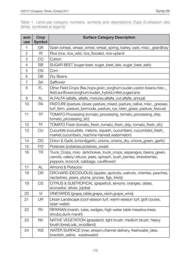
Crops and Land-use Categories. Daily water balance is the key component of the ETaw model. The calculations require input of weather or climate data, soil depth and water-holding capacity, crop root depth, and seasonal crop coefficient curves. Because there are thousands of soil and cropping pattern combinations in different cropping seasons, it is impossible to account for all combination in the State. The biggest limitation is the lack of both historical and current cropping pattern information, which has, however, greatly improved in the recent years and refinements are likely in the future. To overcome the problem of too many crop and soil combinations, the crops are separated into 24 land-use categories that consist of individual crops or crops with similar characteristics (Table 1).

Reference Evapotranspiration. Weather and climate data are used to calculate standardized reference evapotranspiration (ETo) for short canopies (Allen et al. 1998; Allen et al., 2005; Monteith, 1965; Monteith and Unsworth, 1990) but there was a lack of solar radiation, humidity, and wind speed data to compute standardized ETo prior to development of CIMIS, i.e. the California Irrigation Management Information System (Snyder and Pruitt, 1995). Since only temperature data were available prior to about 1986, it was decided to use daily maximum and minimum temperature and the Hargreaves and Samani (1982; 1985) equation to calculate reference evapotranspiration (ETHS) as an approximation for ETo. Using recent climate data from CIMIS, comparisons were made between ETHS and ETo and discrepancies were noted depending on regional climate differences. In general, ETHS was lower than ETo under windy conditions and it was higher than ETo under calm conditions. Using approximately 130 CIMIS weather stations distributed across the State, a 4X4 km grid of correction factors for the ETHS equation was developed. There are many daily temperature and precipitation weather stations in California, but the PRISM data set, which was developed by Oregon State University (PRISM Group, 2011) provided a long-term GIS data base of historical daily maximum and minimum temperature and precipitation on the same 4X4 km grid as the correction factor GIS map. Thus, using the PRISM historical temperature data to compute ETHS and the calibration factors, CALSIMETAW is able to produce ETo estimates on a 4X4 km grid over the State.

115


Table 1. Land-use category numbers, symbols and descriptions (Type d’utilisation des terres, symboles et legend)

and-use

Crop Symbol

Surface Category Description

1 GR Grain (wheat, wheat_winter, wheat_spring, barley, oats, misc._grain&hay

2 RI Rice (rice, rice_wild, rice_flooded, rice-upland

3 CO Cotton

4 SB SUGAR BEET (sugar-beet, sugar_beet_late, sugar_beet_early

5 CN Corn

6 DB Dry Beans

7 SA Safflower

8 FL Other Field Crops (flax,hops,grain_sorghum,sudan,castor-beans,misc._field,sunflower,sorghum/sudan_hybrid,millet,sugarcane

9 AL ALFALFA (alfalfa, alfalfa_mixtures,alfalfa_cut,alfalfa_annual)

10 PA PASTURE (pasture, clover, pasture_mixed, pasture_native, misc._grasses, turf_farm, pasture_bermuda, pasture_rye, klein_grass, pasture_fescue)

11 TP TOMATO Processing (tomato_processing, tomato_processing_drip, tomato_processing_sfc)

12 TF TOMATO Fresh (tomato_fresh, tomato_fresh_drip, tomato_fresh_sfc)

13 CU Cucurbits (cucurbits, melons, squash, cucumbers, cucumbers_fresh_market,cucumbers_machine-harvest,watermelon)

14 OG Onion & Garlic (onion&garlic, onions, onions_dry, onions_green, garlic)

15 PO Potatoes (potatoes,potatoes_sweet

16 TR Truck_Crops_misc (artichokes, truck_crops, asparagus, beans_green, carrots, celery,l ettuce, peas, spinach, bush_berries, strawberries, peppers, broccoli, cabbage, cauliflower)

17 AL Almond & Pistacios

18 OR ORCHARD (DECIDUOUS) (apples, apricots, walnuts, cherries, peaches, nectarines, pears, plums, prunes, figs, kiwis)

19 CS CITRUS & SUBTROPICAL (grapefruit, lemons, oranges, dates, avocados, olives, jojoba)

20 VI VINEYARDS (grape_table,grape_raizin,grape_wine)

21 UR Urban Landscape (cool-season turf, warm-season turf, golf course, open water)

22 RV RIPARIAN (marsh, tules, sedges, high water table meadow,trees, shrubs,duck marsh)

23 NV NATIVE VEGETATION (grassland, light brush, medium brush, heavy brush,forest,oak_woodland)

24 WS WATER SURFACE (river, stream,channel delivery, freshwater_lake, brackish_saline, wastewater)


116

Soils Characteristics and Rooting Depths

A database containing the soil water holding capacity, soil depth, and rooting depth information for all of California was developed from the USDA-NRCS SSURGO database (SSURGO, 2011). The developed database covers all of California on the same 4×4 km grid for all locations that are included in the PRISM database, which covers most of California.

Crop Coefficients. Crop evapotranspiration is estimated as the product of reference evapotranspiration (ETo) and a crop coefficient (Kc) value. Crop coefficients are commonly developed by measuring ETc, calculating ETo, and determining the ratio Kc = ETc / ETo. Most of the crop coefficients used in CALSIMETAW were developed in California. Some were adopted from the literature Doorenbos and Pruitt, (1977) and Allen et al., (1998). While crop coefficients are continuously developed and evaluated, CALSIMETAW was designed for easy updates of both Kc and crop growth information. Also, Kc values need adjustment for microclimates, which are plentiful and extreme in California. A microclimate Kc correction based on the ETo rate is included in the CALSIMETAW model. The Kc values and corresponding growth dates are included by crop in the model. These dates and Kc values are used to estimate daily Kc values during a season.

The State is separated into 272 detailed analysis unit (DAU) regions based on watershed and other factors related to water transfer and use within the region. Crop surveys are periodically completed within each DAU by DWR staff, and the percentages of individual crops within a multiple crop land-use category are known for most DAU regions. Using the percentages of each crop within a DAU, the crop coefficient and growth data are analyzed to determine a weighted mean Kc curve for each crop category. Thus, there are as many as 24 crop category weighted mean Kc curves for each of the DAU regions.

Water Balance Calculations. Although CALSIMETAW has soil characteristic information and computes ETo on a 4X4 km grid, crop planting information is limited to the detailed analysis unit (DAU). Therefore, the DAU is the smallest unit for calculation of the water balance and thus ETaw. Using GIS, a weight mean value is determined by DAU for the soil water holding characteristic, soil depth, root depth, and ETo. The smaller of the soil and root depth and the weighted mean water holding characteristics are used to determine the plant available water (PAW). A 50% allowable depletion is used to estimate the readily available water (RAW) for the effective rooting zone. A management allowable depletion (MAD) is determined by comparing the RAW with the cumulative ETc during the season. The MAD is always less than or equal to RAW, and it is set so that the soil water content at the end of the season is between RAW and PAW.

Weighted crop coefficient curves for each land-use category are used with the daily ETo estimates to calculate daily ETc. The ETc is subtracted from the soil water content on each day until the soil water depletion (SWD) exceeds the MAD. Then an irrigation is applied and the soil water depletion goes back to zero (i.e. back to field capacity). Similarly, rainfall will decrease the soil water depletion to zero but never negative. When rainfall depths are greater than the SWD, the rainfall is effective only up to a depth equal to SWD. There is no correction for runoff or runon to the field. It is assumed that if rainfall is sufficient to have appreciable runoff, then the soil will be filled to field capacity and our assumption that effective rainfall cannot exceed SWD still applies. This method works because the water balance calculations are daily. It might fail for intervals longer than a day.

117


Fig. 1. Fluctuations in soil water content (SWC) between field capacity (FC) and maximum soil water content (SWCx) over the period of one year (Evolution du contenu en eau du sol (SWC) entre la capacité au champs (FC) et le contenu maximum en eau (SWCx) sur la période d’un an)

Real-time CALSIMETAW. CALSIMETAW provides a method to analyze historical data to determine trends in agricultural water demand, but it is also useful for near real-time demand estimates. The CIMIS weather network for estimating ETo is operated by DWR, and recently, DWR and the University of California (UC) Davis developed a new map product called “Spatial CIMIS”, which is available and explained on the CIMIS website (CIMIS, 2011). Although there are about 130 CIMIS weather stations in California, many locations have limited weather data for ETo estimation, so there are gaps in the spatial data. To resolve this problem, DWR and UC Davis used satellite data to estimate solar radiation between stations and algorithms to estimate changes in temperature, humidity, and wind speed between stations. The result is spatial CIMIS, which provides spatial ETo estimation over the State. CALSIMETAW uses GIS to incorporate the spatial ETo estimates into the program and provide daily maps of crop ETc over the State. Forecast CALSIMETAW. In cooperation with DWR and UC Davis, the National Weather Service (NWS) has developed an ETo forecast product that is currently available in much of California. DWR and UC Davis are working with the NWS to incorporate this forecast ETo into the CALSIMETAW model. This will provide useful information to hydrologists who manage the canal system in California and could improve management of the Sacramento – San Joaquin River Delta.


118

Climate Change. The ability to adjust for climate change impacts on evapotranspiration and more importantly water balance are included in the CALSIMETAW model. The model includes a weather generator that provides 30 or more years of simulated daily weather data from monthly inputs. Statistics from the generated data are nearly identical to observed data. The simulated data are used like observed data to compute ETo and estimate ETc. To study climate change, one only needs to change the monthly mean climate variables to the projected climate. The program adjusts for radiation, temperature, humidity, wind speed, and carbon dioxide concentration. Of course, a bigger effect on irrigated agriculture is the expected change in precipitation. Changing the input monthly precipitation data will result in different precipitation patterns and CALSIMETAW will indicate if the demand for irrigation water will change due to the precipitation changes. Thus, CALSIMETAW does allow for the input of projected climate change and it will provide information on agricultural water demand in the new scenario.

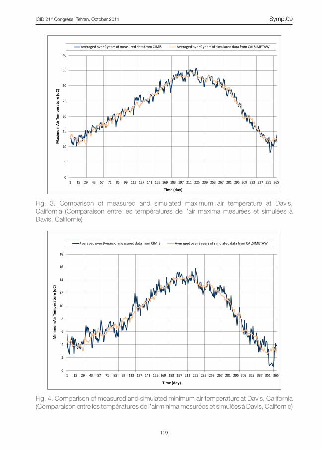
Simulation Accuracy. To test the accuracy of CALSIMETAW, nine years of daily measured weather data (1990–1998) from the California Irrigation Management Information System (CIMIS) in Davis were used in the model to simulate 30 years of daily weather data. The weather data consist of Rs, Tmax, Tmin, wind speed, Tdew, and rainfall. The weather data simulated from CALSIMETAW were compared with the data from CIMIS. Figures 2, 3, 4, and 5 illustrate that Rs, Tmax, Tmin, and SIMETAW predicted ETo values were well correlated with those values obtained from CIMIS. Similar results were observed for rainfall, wind speed, and Tdew data.

Fig. 2. Comparison of measured and simulated solar radiation at Davis, California (Compraison entre la radiation solaire mesurée et simulée à Davis, Californie)

119


Fig. 3. Comparison of measured and simulated maximum air temperature at Davis, California (Comparaison entre les températures de l’air maxima mesurées et simulées à Davis, Californie)

Fig. 4. Comparison of measured and simulated minimum air temperature at Davis, California (Comparaison entre les températures de l’air minima mesurées et simulées à Davis, Californie)


120

Fig. 5. Comparison of estimated and simulated reference evapotranspiration at Davis, California (Comparaison entre l’évapotranspiration de référence mesurée et simulée à Davis, Californie)

Application Software. The CALSIMETAW application model was written using Microsoft C# for numerical calculations, graphics, etc. and Oracle software for data storage.

3. WEAP APPLICATION

Model Overview. WEAP (Water Evaluation and Planning) model is a fully integrated water resources system analysis tool. It is a physically-based simulation model that integrates water demands from all sectors directly with the elements of water supply such as rivers, reservoirs, canals, groundwater, desalination and hydropower projects (Yates et al. 2005). It uses a rainfall-runoff “catchment” module which simulates hydrologic processes including surface runoff, subsurface interflow and baseflow, deep percolation, surface-ground water interaction, root zone soil moisture, and irrigation demand based on crop ET. This integration of watershed hydrology with water planning process makes WEAP particularly suitable to evaluate the potential impacts of climate change both on water demand and supply of a region’s water management project in a single tool.

Another important feature of WEAP is the ability to build and organize multiple scenarios with ease. Scenarios are a range of alternative futures which can address a broad range of “what if” questions. They are designed to deal with uncertainties inherent in the future which are beyond the control of water managers. For example, WEAP can be used to evaluate future impacts of changes in land use, demographics, socioeconomics, and climate. Once,

121


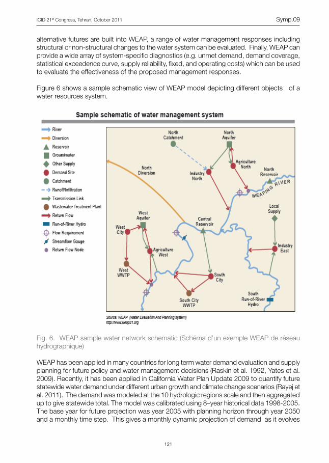
alternative futures are built into WEAP, a range of water management responses including structural or non-structural changes to the water system can be evaluated. Finally, WEAP can provide a wide array of system-specific diagnostics (e.g. unmet demand, demand coverage, statistical exceedence curve, supply reliability, fixed, and operating costs) which can be used to evaluate the effectiveness of the proposed management responses.

Figure 6 shows a sample schematic view of WEAP model depicting different objects of a water resources system.

Fig. 6. WEAP sample water network schematic (Schéma d’un exemple WEAP de réseau hydrographique) WEAP has been applied in many countries for long term water demand evaluation and supply planning for future policy and water management decisions (Raskin et al. 1992, Yates et al. 2009). Recently, it has been applied in California Water Plan Update 2009 to quantify future statewide water demand under different urban growth and climate change scenarios (Rayej et al. 2011). The demand was modeled at the 10 hydrologic regions scale and then aggregated up to give statewide total. The model was calibrated using 8–year historical data 1998-2005. The base year for future projection was year 2005 with planning horizon through year 2050 and a monthly time step. This gives a monthly dynamic projection of demand as it evolves


122

through time, rather than a static snap shot of the future conditions. Below is a narrative description of future scenarios (Source: California Water Plan, Update 2009)

4. FUTURE SCENARIOS

Urban Growth

• Current Trends. Recent trends are assumed to continue into the future. In 2050, nearly 60 million people live in California. The search for affordable housing has drawn families to the interior valleys. Commuters take longer trips in distance and time. In some areas where urban development and natural resources restoration has increased, irrigated cropland has decreased. The state faces lawsuits on a regular basis: from flood damages to water quality and endangered species protections. Regulations are not comprehensive or coordinated, creating uncertainty for local planners and water managers.

• Slow & Strategic Growth. Private, public, and governmental institutions form alliances to provide for more efficient planning and development that is less resource intensive than conditions in the early 21st century. Population growth is slower than projected—about 45 million people live here in 2050. Compact urban development has eased commuter travel. Californians embrace water and energy conservation. Conversion of agricultural land to urban development has slowed and occurs mostly for environmental restoration and flood protection. State government implements comprehensive and coordinated regulatory programs to improve water quality, protect fish and wildlife, and protect communities from flooding.

• Expansive Growth. Development is more resource intensive than conditions in the early 21st century. Population growth is greater than projected with 70 million people living in California in 2050. Families prefer low-density housing, and many seek rural residential properties, expanding urban area boundaries. Where urban development and natural restoration have increased, irrigated crop land has decreased. Some water and energy conservation programs are offered but at a slower rate than trends in the early century. Protection of water quality and endangered species is driven mostly by lawsuits, creating uncertainty for local planners and water managers.

Climate Change. To incorporate the impacts of global warming and climate change on the future water demand, each of the three growth scenarios mentioned above was evaluated under 12 climate scenarios. These climate scenarios were identified by the Governor’s Climate Action Team (CAT) to be used for planning studies in California. The 12 climate scenarios were based on the results of 6 General Circulation Models (GCM) and 2 Greenhouse Gas Emission (GHG) scenarios. These scenarios have distinct estimates of future precipitation and temperature that were used with other factors to estimate future water demands. The 6 climate models were:

• FromFrance:CNRMCM3

• FromUSA:GFDLCM2.1

• FromJapan:MIROC3.2(med)

• FromGermany:MPIECHAM5

• FromUSA:NCARCCSM3

123


• FromUSA:NCARPCM1

These models were chosen on the basis of the availability of detailed outputs for use in various parts of the assessment process and upon consideration of certain aspects of their performance. The results from the 12 future climates were downscaled to the hydrologic regions of California to give time series of future climate (temperature, precipitation) for each of the three urban growth scenarios.

5. FUTURE DEMAND

Future water demand is affected by a number of demographic, socioeconomic and land use factors like population growth, single family and multi-family housing types, family income, water price, urban outdoor landscapes and cropping patterns of agricultural areas. Values of these factors were varied according to scenario themes to test their effects upon the system being analyzed. In this way, scenario analysis is similar to sensitivity analysis, but the scenario analysis tests groups of factors in an organized way.

Together, these factors are used to quantify future water demand for urban, agricultural, and environmental sectors. Each factor is varied between the three scenarios to describe some of the uncertainty that water managers face. For example, the three scenarios use three different, but plausible values of future population when determining future urban water demands. In this section, some of the key factors used to quantify urban, agricultural, and environmental water demands are described.

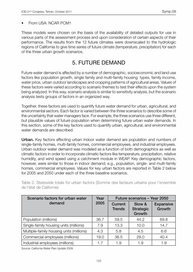
Urban. Key factors affecting urban indoor water demand are population and numbers of single-family homes, multi-family homes, commercial employees, and industrial employees. Urban outdoor water demand was modeled as a function of both demographics as well as climatic factors in order to incorporate climatic factors like temperature, precipitation, relative humidity, and wind speed using a catchment module in WEAP. Key demographic factors, however, were similar to those in indoor demand; e.g., population, single- and multi-family homes, commercial employees. Values for key urban factors are reported in Table 2 below for 2005 and 2050 under each of the three baseline scenarios.

Table 2. Statewide totals for urban factors (Somme des facteurs urbains pour l’ensemble de l’état de Californie)

Scenario factors for urban water demand

Year 2005

Future scenarios – Year 2050Current Trends

Slow & Strategic Growth

Expansive Growth

Population (millions) 36.7 59.5 44.2 69.8Single-family housing units (millions) 7.9 13.3 10.0 14.7Multiple-family housing units (millions) 4.3 5.8 4.5 6.6Commercial employees (millions) 19.0 36.5 28.0 40.4Industrial employees (millions) 1.7 1.9 1.9 1.9

Source: California Water Plan Update 2009


124

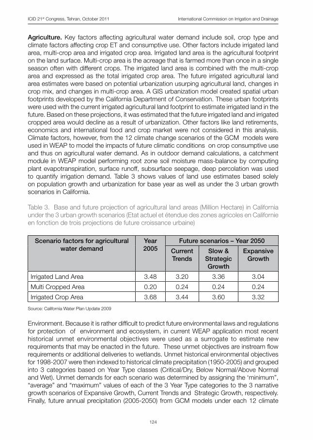
Agriculture. Key factors affecting agricultural water demand include soil, crop type and climate factors affecting crop ET and consumptive use. Other factors include irrigated land area, multi-crop area and irrigated crop area. Irrigated land area is the agricultural footprint on the land surface. Multi-crop area is the acreage that is farmed more than once in a single season often with different crops. The irrigated land area is combined with the multi-crop area and expressed as the total irrigated crop area. The future irrigated agricultural land area estimates were based on potential urbanization usurping agricultural land, changes in crop mix, and changes in multi-crop area. A GIS urbanization model created spatial urban footprints developed by the California Department of Conservation. These urban footprints were used with the current irrigated agricultural land footprint to estimate irrigated land in the future. Based on these projections, it was estimated that the future irrigated land and irrigated cropped area would decline as a result of urbanization. Other factors like land retirements, economics and international food and crop market were not considered in this analysis. Climate factors, however, from the 12 climate change scenarios of the GCM models were used in WEAP to model the impacts of future climatic conditions on crop consumptive use and thus on agricultural water demand. As in outdoor demand calculations, a catchment module in WEAP model performing root zone soil moisture mass-balance by computing plant evapotranspiration, surface runoff, subsurface seepage, deep percolation was used to quantify irrigation demand. Table 3 shows values of land use estimates based solely on population growth and urbanization for base year as well as under the 3 urban growth scenarios in California.

Table 3. Base and future projection of agricultural land areas (Million Hectare) in California under the 3 urban growth scenarios (Etat actuel et étendue des zones agricoles en Californie en fonction de trois projections de future croissance urbaine)

Scenario factors for agricultural water demand

Year 2005

Future scenarios – Year 2050

Current Trends

Slow & Strategic Growth

Expansive Growth

Irrigated Land Area 3.48 3.20 3.36 3.04

Multi Cropped Area 0.20 0.24 0.24 0.24

Irrigated Crop Area 3.68 3.44 3.60 3.32

Source: California Water Plan Update 2009

Environment. Because it is rather difficult to predict future environmental laws and regulations for protection of environment and ecosystem, in current WEAP application most recent historical unmet environmental objectives were used as a surrogate to estimate new requirements that may be enacted in the future. These unmet objectives are instream flow requirements or additional deliveries to wetlands. Unmet historical environmental objectives for 1998-2007 were then indexed to historical climate precipitation (1950-2005) and grouped into 3 categories based on Year Type classes (Critical/Dry, Below Normal/Above Normal and Wet). Unmet demands for each scenario was determined by assigning the ‘minimum”, “average” and “maximum” values of each of the 3 Year Type categories to the 3 narrative growth scenarios of Expansive Growth, Current Trends and Strategic Growth, respectively. Finally, future annual precipitation (2005-2050) from GCM models under each 12 climate

125


scenarios was referenced back to Year Type to give future additional environmental demand over and above the baseline (2005) demand. This was done at each monthly time step in WEAP to give an estimate of future projection of environmental demand over time 2005-2050.

6. RESULTS AND DISCUSSION

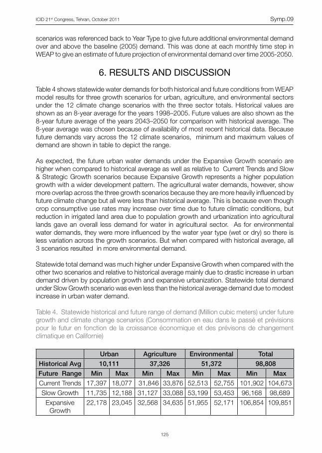
Table 4 shows statewide water demands for both historical and future conditions from WEAP model results for three growth scenarios for urban, agriculture, and environmental sectors under the 12 climate change scenarios with the three sector totals. Historical values are shown as an 8-year average for the years 1998–2005. Future values are also shown as the 8-year future average of the years 2043–2050 for comparison with historical average. The 8-year average was chosen because of availability of most recent historical data. Because future demands vary across the 12 climate scenarios, minimum and maximum values of demand are shown in table to depict the range.

As expected, the future urban water demands under the Expansive Growth scenario are higher when compared to historical average as well as relative to Current Trends and Slow & Strategic Growth scenarios because Expansive Growth represents a higher population growth with a wider development pattern. The agricultural water demands, however, show more overlap across the three growth scenarios because they are more heavily influenced by future climate change but all were less than historical average. This is because even though crop consumptive use rates may increase over time due to future climatic conditions, but reduction in irrigated land area due to population growth and urbanization into agricultural lands gave an overall less demand for water in agricultural sector. As for environmental water demands, they were more influenced by the water year type (wet or dry) so there is less variation across the growth scenarios. But when compared with historical average, all 3 scenarios resulted in more environmental demand.

Statewide total demand was much higher under Expansive Growth when compared with the other two scenarios and relative to historical average mainly due to drastic increase in urban demand driven by population growth and expansive urbanization. Statewide total demand under Slow Growth scenario was even less than the historical average demand due to modest increase in urban water demand.

Table 4. Statewide historical and future range of demand (Million cubic meters) under future growth and climate change scenarios (Consommation en eau dans le passé et prévisions pour le futur en fonction de la croissance économique et des prévisons de changement climatique en Californie)

Urban Agriculture Environmental TotalHistorical Avg 10,111 37,326 51,372 98,808Future Range Min Max Min Max Min Max Min Max

Current Trends 17,397 18,077 31,846 33,876 52,513 52,755 101,902 104,673Slow Growth 11,735 12,188 31,127 33,088 53,199 53,453 96,168 98,689

Expansive Growth

22,178 23,045 32,568 34,635 51,955 52,171 106,854 109,851


126

Because Table 4 only shows the historical and future “average” demand, figures below are given to depict the temporal projection of statewide demand by WEAP model as it steps through time. They are shown for all 3 demand sectors and for 3 growth scenarios under the 12 climate scenarios. The 8 years of actual historical demand data (1998-2005) are also shown for comparison.

1 MAF = 1233 Million cubic meters Source: California Water Plan Update 2009

Fig. 7. Statewide water demand under 12 climate change scenarios (Demande en eau dans l’état de Californie en fonction de 12 hypothèses de changement climatique)

127


As shown in the three figures below, environmental demand tops agricultural demand followed by urban sector in all 3 growth scenarios. Although, urban sector demand increases over time due to population growth and urbanization in all 3 growth scenarios, but Expansive Growth showed a faster rate of increase as expected. Because climate factors impacted only the outdoor portion of the urban demand, variability across the 12 climate change scenarios on total urban sector is less visible. Also shown in these figures, agricultural demand shows decline over time due to decline in irrigated lands as a result of urbanization and urban encroachment into agricultural lands. This decline in irrigated lands was such that it overshadowed the rise in evapotranspiration and crop water use rates due to warming trend in climate over time, resulting in agricultural water demand “volume” to decline following the declining pattern of irrigated lands over time. Variability across the 12 climate change scenarios, however, was more apparent in agricultural sector than in Urban sector as shown in the figures below. This was because climate factors were key factors in determining demand in agricultural sector. Environmental demand on the other hand increased little over time when compared with urban and agricultural sector for all three growth scenarios. This was because instream flow was the major component of environmental sector demand and was more influenced by the year type (wet or dry) so there was less variations across the was growth scenarios.

7. SUMMARY AND CONCLUSIONS

A water resources system evaluation model (WEAP) was used to project future urban, agricultural and environmental demand under 3 urban growth and 12 climate change scenarios as a part of analysis and quantifications required in California Water Plan Update 2009. Three demand sectors; urban, agricultural and environmental were evaluated. The model was applied at the 10 hydrologic regions of State and then the results were aggregated up to give statewide total. Though, the WEAP model can evaluate both the demand and supply side of local or regional water projects, only the demand side was evaluated in this analysis. The effort reported above showed that WEAP is a powerful tool in building multiple scenarios to project the future demand under various urban growth and climate change scenarios. This gives a dynamic time-varying level of demand as it evolves over time, rather than a static future level. The results showed future urban water demands increased with rapid pace under the three growth scenarios and were heavily influenced by the assumptions of future population growth and to a lesser extent by future climate. Future agricultural water demands, however, declined mainly because of decline in agricultural lands due to urbanization but were heavily influenced by future climate conditions across the 12 climate scenario examined. Environmental water demands were more influenced by the year type (wet or dry) so there is less variation across the three growth scenarios.

REFERENCES

Allen, R.G., Pereira, L.S., Raes, D., and Smith, M., 1998. Crop evapotranspiration: Guidelines for computing crop water requirements. FAO Irrigation and Drainage Paper 56, FAO, Rome.

Allen, R.G., Walter, I.A., Elliott, R.L., Howell, T.A., Itenfisu, D., Jensen, M.E. and Snyder, R.L. 2005. The ASCE Standardized Reference Evapotranspiration Equation. Amer. Soc. of Civil Eng. Reston, Virginia. 192p.


128

California Department of Water Resources, California Water Plan Update 2009. http://www.waterplan.water.ca.gov/cwpu2009.

CIMIS (2011). Spatial CIMIS. http://wwwcimis.water.ca.gov/cimis/cimiSatOverview.jsp

Doorenbos, J. and Pruitt, W.O. 1977. Guidelines for predicting crop water requirements. FAO Irrigation and Drainage Paper 24, FAO, Rome.

Hargreaves, G.H., and Samani, Z.A. (1982). “Estimating potential evapotranspiration.” Tech. Note, J. Irrig. and drain. Engrg., ASCE, 108(3):225-230.

Hargreaves, G.H., and Samani, Z.A. (1985). “Reference crop evapotranspiration from temperature.” Applied Eng. in Agric., 1(2):96-99.

Monteith, J. L., 1965. Evaporation and Environment. 19th Symposia of the Society for Experimental Biology, University Press, Cambridge, 19:205-234.

Monteith, J. L. and Unsworth, M. H. 1990. Principles of Environmental Physics, 2nd ed., Edward Arnold, London.

PRISM. Oregon State University. http://prism.oregonstate.edu/

Raskin, P., Hansen, E. and Zhu, Z. 1992. Simulation of water supply and demand in the Aral Sea Region. Water Int. 17, 55-67.

Rayej, M., Juricich, R., Groves, D., Yates, D., 2011. Scenarios of future California water demand through 2050: Growth and Climate Change. World Environmental and Water Resources Congress, Palm Spring, California, May 2011.

SSURGO, 2011. Soil Survey Geographic (SSURGO) Database. USDA NRCS http://soils.usda.gov/survey/geography/ssurgo/

Yates, D., Sieber, J., Purkey, D., and Huber Lee, A. 2005a. WEAP21: A demand priority and preference driven planning model. Part 1: Model characteristics. Water Int. 30, 487-500.

Yates, D., Sieber, J., Purkey, D., and Huber-Lee, A. and Galbraith H. 2005b. WEAP21: A demand priority and preference driven planning model. Part 2: Aiding freshwater ecosystem service evaluation. Water Int. 30, 501-512.

Yates, D., Purkey D., Sieber J., Huber-Lee A., Galbraith H., West, J., Herrod-Julius, S., Young C., Joyce B. and Rayej, M. 2009. Climate driven water resources model of the Sacramento basin. Journal of Water Resources Planning and Management, American Society of Civil Engineers, Vol. 135 (5), 303-313.

calsimetaw and weap models for water...

Documents