calculus - school of mathematicsppmartin/learn/calculus/calcbk.pdf · we assume that you have...
TRANSCRIPT

Calculus
P P Martin
November 19, 2006

2
Contents
1 Introduction 5
1.1 Review of Differentiation . . . . . . . . . . . . . . . . . . . . . 5
1.1.1 Functions . . . . . . . . . . . . . . . . . . . . . . . . . 5
1.1.2 Limits . . . . . . . . . . . . . . . . . . . . . . . . . . . 6
1.1.3 Differentiation . . . . . . . . . . . . . . . . . . . . . . . 7
1.2 Other things we expect you to know! . . . . . . . . . . . . . . 7
1.3 Other support material . . . . . . . . . . . . . . . . . . . . . . 8
2 Functions of more than one variable 9
2.1 Introduction . . . . . . . . . . . . . . . . . . . . . . . . . . . . 9
2.2 Partial Differentation . . . . . . . . . . . . . . . . . . . . . . . 10
2.2.1 Higher derivatives . . . . . . . . . . . . . . . . . . . . . 11
2.3 Chain Rule . . . . . . . . . . . . . . . . . . . . . . . . . . . . 12
2.4 Maxima and Minima . . . . . . . . . . . . . . . . . . . . . . . 12
2.4.1 Several variables . . . . . . . . . . . . . . . . . . . . . 15
2.5 Lagrange Multipliers . . . . . . . . . . . . . . . . . . . . . . . 16
2.6 Taylor series . . . . . . . . . . . . . . . . . . . . . . . . . . . . 20
2.7 Further Notes and Exercises . . . . . . . . . . . . . . . . . . . 22
3 Multiple integration 25
3.1 Ordinary integration revisited . . . . . . . . . . . . . . . . . . 25
3.2 Multiple integration . . . . . . . . . . . . . . . . . . . . . . . . 26
3.3 Further Notes and Exercises . . . . . . . . . . . . . . . . . . . 30
3

4 CONTENTS
3.4 Polar coordinates . . . . . . . . . . . . . . . . . . . . . . . . . 32
3.5 General change of variables . . . . . . . . . . . . . . . . . . . 34
3.6 Spherical polar coordinates . . . . . . . . . . . . . . . . . . . . 35
3.7 Examples and Exercises . . . . . . . . . . . . . . . . . . . . . 37
3.7.1 Actuarial Science, Quantity and Physics . . . . . . . . 37
3.7.2 Integration related examples . . . . . . . . . . . . . . . 40
4 Differential Equations 43
4.1 Solutions I . . . . . . . . . . . . . . . . . . . . . . . . . . . . . 44
4.1.1 Homogeneous Linear DEs . . . . . . . . . . . . . . . . 45
4.1.2 Inhomogeneous DEs . . . . . . . . . . . . . . . . . . . 47
4.2 Wronskians, Variation etc. . . . . . . . . . . . . . . . . . . . . 49
4.3 General linear second order equations . . . . . . . . . . . . . . 50
4.4 Series solution methods . . . . . . . . . . . . . . . . . . . . . . 52
5 Laplace Transforms 55
5.1 Inverse operator . . . . . . . . . . . . . . . . . . . . . . . . . . 56
5.2 Transforms of differentials . . . . . . . . . . . . . . . . . . . . 57
5.3 Solution of Ordinary Differential Equations . . . . . . . . . . . 57
6 More exercises 61
Chapter 1
Introduction
We assume that you have attended a first year calculus course. This would
have covered topics such as Limits, Continuity and Differentiability for func-
tions of one variable. Just in case you are feeling rusty, here is a brief review.
1.1 Review of Differentiation
We will need to recall the notions of Function, Limit, and Differentiation.
1.1.1 Functions
There are many kinds of function, and a formal mathematical definition can
be given which encompasses them all. You may know it. For our purposes it
will be sufficient to start by thinking about real functions of real variables.
A real function is something which takes as input a real
number, and gives as output another real number.
There are all sorts of special cases. None of the special cases we will need
are any cause for alarm!
Example 1.1.
f(x) = x2
5
6 CHAPTER 1. INTRODUCTION
Example 1.2.
f(x) = sin(x)
1.1.2 Limits
Some functions f(x) break down at certain values of x.
Example 1.3. Consider
f(x) = x−1
at x = 0!
Other functions have similar looking problems at certain values of x, but
can usefully be studied by using the notion of limit.
A function f(x) has a limit l at x = c (c some given
constant),
if we can make the value of f(x) − l arbitrarily small,
by choosing x suitably close to c.
We write
limx→c
f(x) = l
if such a limit exists.
The function f(x) = x−1 has no limit at x = 0. The closer we get to
x = 0, the bigger it gets, without bound! We say f(x) is divergent at x = 0.
However,
Example 1.4. Consider
f(x) = x−1 sin(x)
at x = 0. Again there is a problem, caused by the x−1 part. We can see that
the sin(x) part, which gets small close to x = 0, might restrain this divergence,
but we can’t tell just by staring at it! In fact, by carefully calculating the
value of this function for values of x close to (but not at) 0 we can see that
limx→0
f(x) = 1
1.2. OTHER THINGS WE EXPECT YOU TO KNOW! 7
1.1.3 Differentiation
Not every function can be differentiated. If a function can be differentiated
(at x), the differential is given by
df(x)
dx= lim
h→0
f(x + h) − f(x)
h
Note that this is exactly what we mean by the tangent to the curve of the
graph of f(x) at x.
Example 1.5. For
f(x) = x2
we get
df(x)
dx= lim
h→0
(x + h)2 − x2
h= lim
h→0
2xh + h2
h
= limh→0
2xh
h+ lim
h→0
h2
h= 2x
(I hope this is what you were expecting!)
1.2 Other things we expect you to know!
de Moivre’s theorem etc.:
eiθ = cos θ + i sin θ
so
(cos θ + i sin θ)n = cos nθ + i sin nθ
so, for example,
cos 2θ = cos2 θ − sin2 θ = 2 cos2 θ − 1 (1.1)

8 CHAPTER 1. INTRODUCTION
1.3 Other support material
Check out the course homepage.
Check out the vast amount of related material on the web.
Check out past exam papers and solutions.
Check out books called ‘CALCULUS’ (or similar); such as the SCHAUM
OUTLINE SERIES book on this topic, and other books mentioned on the
course homepage.
Check out ‘Mathematical Methods for Science Students’ by G Stephenson
(Longman). 1
Check out the DERIVE mathematical software package.
1Some of the examples in the present draft of this work are taken from my own un-
dergraduate Calculus notes (from a course given by the legendary Dr Ian Ketley). This
means that they are inspired by, or directly taken from, examples and exercises to be found
in Stephenson’s excellent book. As a result, the present version of this work is possibly
suitable only for its present educational purpose, and not for publication or any other form
of redistribution. Buy Stephenson’s book.
Chapter 2
Functions of more than one
variable
2.1 Introduction
If we collate the data from enough actuarial tables (say), we can construct
a function which, when we input the age of a person in years, returns the
probability that they will have a serious illness within the next twelve months.
This is, potentially, a very useful function to help assess risk in health
insurance.
Of course it is a very crude model of the health profile of any given
candidate for insurance. There are a number of other factors which directly
affect the probability of illness, besides age. For example, the number of
cigarettes smoked each day.
Based on this and countless other examples it will be obvious that func-
tions which model aspects of real life are likely to need to be models with
more than one input parameter. That is, functions of more than one variable.
Example 2.1.
f(x, y) = x2 − 2xy
9
10 CHAPTER 2. FUNCTIONS OF MORE THAN ONE VARIABLE
2.2 Partial Differentation
The graph of a function f(x, y) has two base axes (x, y) and a value axis f .
This makes it difficult to draw on the page, but the concept is just the same
as for graphing f(x). Such functions can have maxima, and minima, and it
is very useful to be able to locate these features.
Finding the maxima and minima of ordinary funtions is one of the jobs
which differentiation helps us enormously with, as we know. Is there some
version of differentiation we can use for f(x, y)?
There are two partial derivatives:
fx =∂f
∂x= lim
h→0
f(x + h, y) − f(x, y)
h
fy =∂f
∂y= lim
h→0
f(x, y + h) − f(x, y)
h
Note that in each case we pick a variable to differentiate with respect to,
and then differentiate treating the other variable as if it were a constant.
Example 2.2. We can’t differentiate f(x, y) = x2−2xy in the ordinary way,
but if we fix y = 3 (say), then f(x, 3) = x2 − 6x, which we can differentiate.
We can do it again for any other ‘fixed’ value of y. All these differentiations
can be summarized by the partial differentiation with respect to x:
fx = 2x − 2y.
Similarly
fy = −2x.
Note that the differentiated function can still be a function of one or more
variables!
Example 2.3. Yes, that’s right
∂x2
∂y= 0.
Here we are holding x constant, so we are differentiating a constant!
2.2. PARTIAL DIFFERENTATION 11
Exercise 2.4.
f(x, y) = sin2(x) cos(x) +x
y2
Determine fx and fy.
2.2.1 Higher derivatives
Any function may, in principle, be differentiated. The output of the opera-
tion of differentiating a function is another function, so we may differentiate
multiple times. The same idea works for partial differentiation.
The notion is straightfoward! What we have to grasp is really just nota-
tion.
fxx =∂2f
∂x2=
∂
∂xfx =
∂
∂x
(∂f
∂x
)
fyy =∂2f
∂y2=
∂
∂yfy =
∂
∂y
(∂f
∂y
)
fxy = fyx ==∂2f
∂xy=
∂
∂xfy =
∂
∂x
(∂f
∂y
)
(In this last one we have been a bit glib. Think about it!)
These are the second derivatives. Higher derivatives work similarly.
Example 2.5. For
f(x, y) = x2 − 2xy
then
fxx = 2
fyy = 0
fxy = −2
fxxxx = 0

12 CHAPTER 2. FUNCTIONS OF MORE THAN ONE VARIABLE
2.3 Chain Rule
Suppose
z = f(x, y)
given, but
x = x(r, s)
y = y(r, s)
How do we compute ∂z∂r
? (Compare this with the similar problem for the
one–variable case.)
Answer:∂z
∂r=
∂f
∂x
∂x
∂r+
∂f
∂y
∂y
∂r
(and similarly for s).
Exercise 2.6. Verify that this reduces to the usual one–variable case.
Example 2.7.
z = x3 + y3
where
x = 2r + s
y = 3r − 2s
Find ∂z∂r
, ∂z∂s
1
2.4 Maxima and Minima
We can find the maxima of f(x) by differentiation, but the underlying def-
inition is more straightforward. The point x = c is a (local) maximum of
1Partial answer:∂z
∂r= 6(2r + s)2 + 9(3r − 2s)2

2.4. MAXIMA AND MINIMA 13
f(x) if the value of f(x) is lower than f(c) for every point in the immediate
neighbourhood of x = c.
This definition generalises in a simple way to f(x, y).
A point (x, y) = (c, d) is a maximum of f(x, y) if the
value of f(x, y) is lower than f(c, d) for every point in
the immediate neighbourhood of (c, d).
Here is a picture of a simple mountain. The maximum is the highest
point.
y
(x,y)
x
f
0
The coordinate system in this picture is not intrinsic to the mountain. It
is something we put on so that we can give the location of the maximum, and
other features, in a convenient format. Once we have a coordinate system we
can, in principle, give the height of the mountain at each point of the (x, y)
base plane.
This height function will thus be a function of two variables.
Given this function, f(x, y) say, how do we find the maximum (mini-
mum)?
Once again consider f(x, y) as a function of one variable by holding y
constant. If f(x, y) is a maximum at, say, (x, y) = (xc, yc) (xc, yc given
constants), it is also a maximum of the function f(x, yc).
14 CHAPTER 2. FUNCTIONS OF MORE THAN ONE VARIABLE
Thus a necessary condition for an extremum is
fx = fy = 0
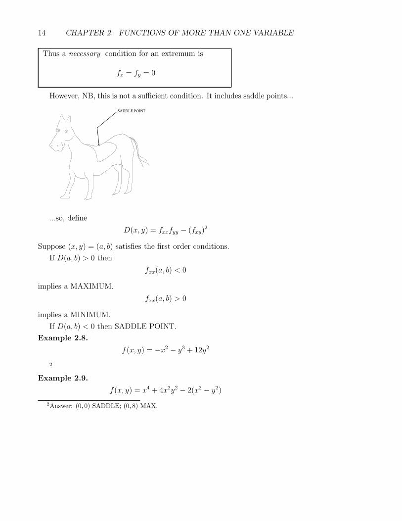
However, NB, this is not a sufficient condition. It includes saddle points...
SADDLE POINT
...so, define
D(x, y) = fxxfyy − (fxy)2
Suppose (x, y) = (a, b) satisfies the first order conditions.
If D(a, b) > 0 then
fxx(a, b) < 0
implies a MAXIMUM.
fxx(a, b) > 0
implies a MINIMUM.
If D(a, b) < 0 then SADDLE POINT.
Example 2.8.
f(x, y) = −x2 − y3 + 12y2
2
Example 2.9.
f(x, y) = x4 + 4x2y2 − 2(x2 − y2)
2Answer: (0, 0) SADDLE; (0, 8) MAX.
2.4. MAXIMA AND MINIMA 15
3
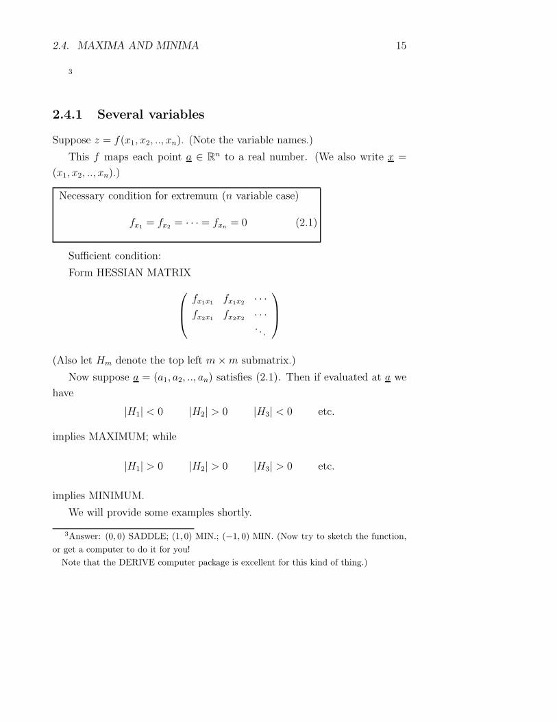
2.4.1 Several variables
Suppose z = f(x1, x2, .., xn). (Note the variable names.)
This f maps each point a ∈ Rn to a real number. (We also write x =
(x1, x2, .., xn).)
Necessary condition for extremum (n variable case)
fx1= fx2
= · · · = fxn = 0 (2.1)
Sufficient condition:
Form HESSIAN MATRIX
fx1x1fx1x2
· · ·fx2x1
fx2x2· · ·. . .
(Also let Hm denote the top left m × m submatrix.)
Now suppose a = (a1, a2, .., an) satisfies (2.1). Then if evaluated at a we
have
|H1| < 0 |H2| > 0 |H3| < 0 etc.
implies MAXIMUM; while
|H1| > 0 |H2| > 0 |H3| > 0 etc.
implies MINIMUM.
We will provide some examples shortly.
3Answer: (0, 0) SADDLE; (1, 0) MIN.; (−1, 0) MIN. (Now try to sketch the function,
or get a computer to do it for you!
Note that the DERIVE computer package is excellent for this kind of thing.)

16 CHAPTER 2. FUNCTIONS OF MORE THAN ONE VARIABLE
2.5 Lagrange Multipliers
Problem:
Maximize f(x1, x2) subject to a constraint on the allowable values of
x1, x2, let us say of the form g(x1, x2) = k, where g is a given function and k
a constant.
(Typically an analyst might be asked to determine the production pa-
rameters for a company so as to maximize profit.
Suppose the company makes TVs and RADIOs, and the profit function
depends on the number of each made.
Naively we maximize profit by making infinitely many of each, but of
course there will be practical limitations on the total number of devices which
can be produced in the real world factory.
We want to maximize subject to these realistic constraints.)
Solution:
Form
L(x1, x2, λ) = f(x1, x2) − λ[g(x1, x2) − k]
(λ is called the LAGRANGE MULTIPLIER.)
Now find unconstrained maximum of L:
Necessary:
Lx1= Lx2
= Lλ = 0
(Note that the last condition enforces the original constraint!)
Example 2.10.
f(x1, x2) = 25 − x21 − x2
2
subject to
2x1 + x2 = 4
so
L = 25 − x21 − x2
2 − λ[2x1 + x2 − 4]
Lx1= −2x1 − 2λ
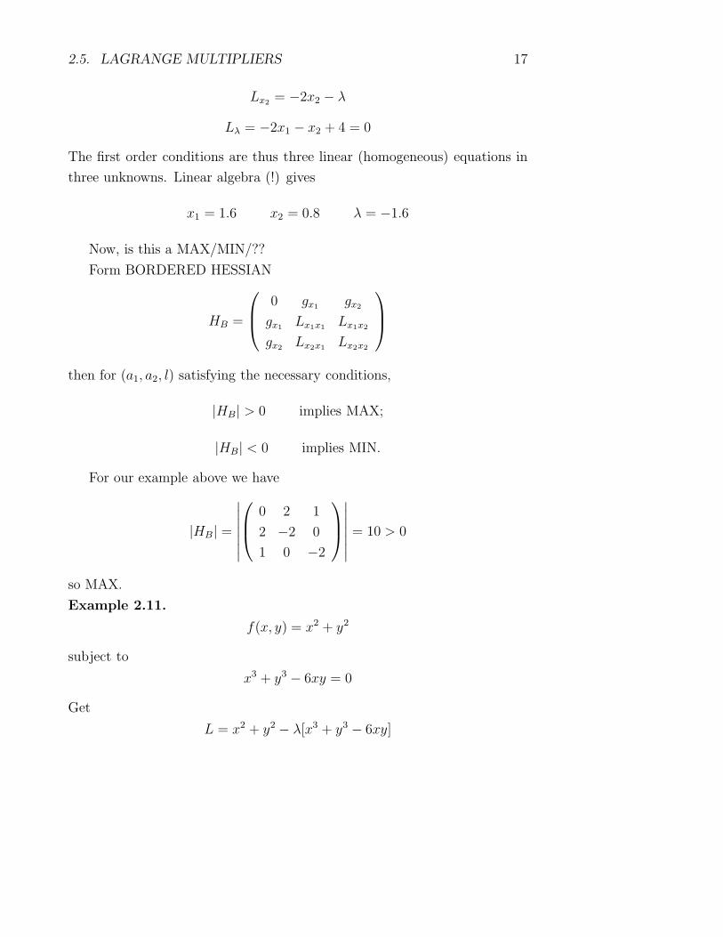
2.5. LAGRANGE MULTIPLIERS 17
Lx2= −2x2 − λ
Lλ = −2x1 − x2 + 4 = 0
The first order conditions are thus three linear (homogeneous) equations in
three unknowns. Linear algebra (!) gives
x1 = 1.6 x2 = 0.8 λ = −1.6
Now, is this a MAX/MIN/??
Form BORDERED HESSIAN
HB =
0 gx1gx2
gx1Lx1x1
Lx1x2
gx2Lx2x1
Lx2x2
then for (a1, a2, l) satisfying the necessary conditions,
|HB| > 0 implies MAX;
|HB| < 0 implies MIN.
For our example above we have
|HB| =
∣∣∣∣∣∣∣
0 2 1
2 −2 0
1 0 −2
∣∣∣∣∣∣∣
= 10 > 0
so MAX.
Example 2.11.
f(x, y) = x2 + y2
subject to
x3 + y3 − 6xy = 0
Get
L = x2 + y2 − λ[x3 + y3 − 6xy]

18 CHAPTER 2. FUNCTIONS OF MORE THAN ONE VARIABLE
Necessary conditions:
Lx = 2x − 3x2λ + 6yλ = 0 (2.2)
Ly = 2y − 3y2λ + 6xλ = 0 (2.3)
Lλ = −(x3 + y3 − 6xy) = 0
Together (2.2) and (2.3) imply
λ =2x
3x2 − 6y=
2y
3y2 − 6x
so
x2y − xy2 + 2x2 − 2y2 = 0
so
(x − y)(2x + 2y + xy) = 0
Evidently x = y is a solution to this. Substitute back into the constraint:
2x3 − 6x2 = 0
with solutions x = 0, 3.
So, we have (0, 0) (a MINIMUM) and (3, 3) (a local MAXIMUM).
(Sketch the curve implied by the constraint to confirm this.)
Example 2.12. In a suitable coordinate system, the Chicago Beltway lies
on the curve
3(x2 + y2) + 4xy = 2
You are tendering for the job of building a connecting road from the Beltway
to Soldier Field sports stadium (at coordinates (0,0)).
It costs your company $5× 10⁷ per kilometre to build road. What is the
minimum tender you could bid without making a loss?4
4Answer: (±1√5, ±1√
5) min.; (±1,∓1) max., so $
√2
5.5.107.

2.5. LAGRANGE MULTIPLIERS 19
Figure 2.1: Plot of x3 + y3 − 6xy = 0 in the interval −4 < x, y < 4.
Figure 2.2: Plot of 3x2 + 3y2 + 4xy = 2 in the interval −4 < x, y < 4.
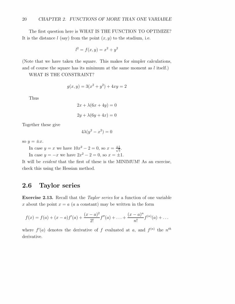
20 CHAPTER 2. FUNCTIONS OF MORE THAN ONE VARIABLE
The first question here is WHAT IS THE FUNCTION TO OPTIMIZE?
It is the distance l (say) from the point (x, y) to the stadium, i.e.
l2 = f(x, y) = x2 + y2
(Note that we have taken the square. This makes for simpler calculations,
and of course the square has its minimum at the same moment as l itself.)
WHAT IS THE CONSTRAINT?
g(x, y) = 3(x2 + y2) + 4xy = 2
Thus
2x + λ(6x + 4y) = 0
2y + λ(6y + 4x) = 0
Together these give
4λ(y2 − x2) = 0
so y = ±x.
In case y = x we have 10x2 − 2 = 0, so x = ±1√5.
In case y = −x we have 2x2 − 2 = 0, so x = ±1.
It will be evident that the first of these is the MINIMUM! As an exercise,
check this using the Hessian method.
2.6 Taylor series
Exercise 2.13. Recall that the Taylor series for a function of one variable
x about the point x = a (a a constant) may be written in the form
f(x) = f(a) + (x − a)f ′(a) +(x − a)2
2!f ′′(a) + . . . +
(x − a)n
n!f (n)(a) + . . .
where f ′(a) denotes the derivative of f evaluated at a, and f (n) the nth
derivative.
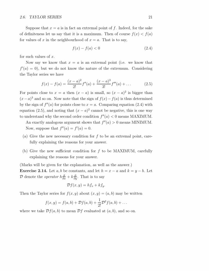
2.6. TAYLOR SERIES 21
Suppose that x = a is in fact an extremal point of f . Indeed, for the sake
of definiteness let us say that it is a maximum. Then of course f(x) < f(a)
for values of x in the neighbourhood of x = a. That is to say,
f(x) − f(a) < 0 (2.4)
for such values of x.
Now say we know that x = a is an extremal point (i.e. we know that
f ′(a) = 0), but we do not know the nature of the extremum. Considering
the Taylor series we have
f(x) − f(a) =(x − a)2
2!f ′′(a) +
(x − a)3
3!f ′′′(a) + . . . (2.5)
For points close to x = a then (x − a) is small, so (x − a)2 is bigger than
(x−a)3 and so on. Now note that the sign of f(x)− f(a) is thus determined
by the sign of f ′′(a) for points close to x = a. Comparing equation (2.4) with
equation (2.5), and noting that (x − a)2 cannot be negative, this is one way
to understand why the second order condition f ′′(a) < 0 means MAXIMUM.
An exactly analogous argument shows that f ′′(a) > 0 means MINIMUM.
Now, suppose that f ′′(a) = f ′(a) = 0.
(a) Give the new necessary condition for f to be an extremal point, care-
fully explaining the reasons for your answer.
(b) Give the new sufficient condition for f to be MAXIMUM, carefully
explaining the reasons for your answer.
(Marks will be given for the explanation, as well as the answer.)
Exercise 2.14. Let a, b be constants, and let h = x − a and k = y − b. Let
D denote the operator h ∂∂x
+ k ∂∂y
. That is to say
Df(x, y) = hfx + kfy.
Then the Taylor series for f(x, y) about (x, y) = (a, b) may be written
f(x, y) = f(a, b) + Df(a, b) +1
2!D2f(a, b) + . . .
where we take Df(a, b) to mean Df evaluated at (a, b), and so on.
22 CHAPTER 2. FUNCTIONS OF MORE THAN ONE VARIABLE
(a) Show that the usual necessary condition for an extremal point of f(x, y)
at (a, b) implies Df(a, b) = 0.
(b) Write out explicitly what is meant by the shorthand D2f(a, b).
(c) Hence derive the usual full second order condition for a maximum at
(a, b).
Exercise 2.15. OPTIONAL: By considering the above two exercises to-
gether, think about how to proceed to investigate the nature of extremal
points f(a, b), when the quatities evaluated in the second order test (as de-
fined in section 2.4 of the notes) turn out to vanish.
Another exercise relevant for this section is Exercise 6.1 below.
2.7 Further Notes and Exercises
Exercise 2.16. The trajectory through space of a 150 x 106 kg chunk of
cosmic debris lies in a plane through the Earth. Suitably coordinatizing this
plane, with the centre of the Earth at the point (0, 0), the trajectory is given
by the curve
x2 + 8xy + 7y2 − 225 = 0
(units are thousands of kilometres). What is the closest distance which the
object comes to the Earth?
(HINT: Use the method of Lagrange multipliers. What is the function to be
minimized? What is the constraint equation? Give a sketch of the trajectory
if it helps you to envisage the problem and/or check the reasonableness of
your answer.)
OPTIONAL: Is it safe for your company to insure against damage result-
ing from the passage of this object?
Exercise 2.17. Using the method of Lagrange’s multipliers, find the shortest
distance from the point P (0, 0, 1) on the z-axis, to the curve y3+x3+y2+x2 =
0 which lies in the (x, y)-plane.

2.7. FURTHER NOTES AND EXERCISES 23
Exercise 2.18.
1. Find all the stationary points (maxima, minima and saddle points) of
the function
g(x, y) = x2y2.
2. Show that the function
f(x, y) = −xy e−x2
+y2
2
has a stationary point at x = 0, y = 0.
Find all the other stationary points of f(x, y).
Determine the nature of the stationary point at (0, 0).
The next few exercises really are just that, i.e. relatively routine opti-
misation problems designed to build up your mathematical ‘muscles’. They
can all be solved simply by other means, but the point here is to practice
Lagrange multipliers!
Exercise 2.19. Find all the stationary points of the function
g(x, y) = x2 + y2
subject to
x2 + 2y2 = 1
using the method of Lagrange Multipliers. (Check your answer by sketching
the curve defined by the constraint; and separately by elementary substitu-
tion!)
Exercise 2.20. Find all the stationary points of the function
g(x, y) = xy
subject to
x + y − 6 = 0

24 CHAPTER 2. FUNCTIONS OF MORE THAN ONE VARIABLE
using the method of Lagrange Multipliers. (Check your answer by sketching
the curve defined by the constraint; and separately by elementary substitu-
tion!)
Exercise 2.21. Find all the stationary points of the function
g(x, y) = x2 + y2
subject to
x + y − 1 = 0
using the method of Lagrange Multipliers. (Check your answer by sketching
the curve defined by the constraint; and separately by elementary substitu-
tion!)
Chapter 3
Multiple integration
We will start by reviewing ordinary integration. Then we will look at the
meaning and uses of integration, when functions of more than one variable
are involved.
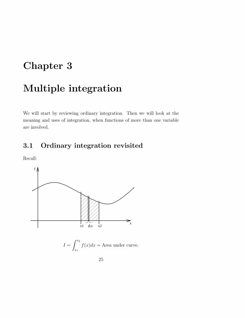
3.1 Ordinary integration revisited
Recall:
x1 x2
f
x∆ x
I =
∫ x2
x1
f(x)dx = Area under curve.
25

26 CHAPTER 3. MULTIPLE INTEGRATION
∼=∑
i
f(xi)∆x
3.2 Multiple integration
Now:
f
x
y
∆ x∆ y
Volume undersurface
Here the generalisation of the usual limits of integration (which define an
interval of the real line — a region of the real line) is an ‘interval’ of the base
plane — a region of the base plane.
Such a thing is more complicated to specify precisely, but the concept is
not so complex.
Let us call the region of the base plane which we are integrating over R.
The volume under the surphace is
I =
∫
R
f(x, y)dR =
∫ ∫
f(x, y)dxdy
∼=∑
i
f(xi, yi) ∆x∆y︸ ︷︷ ︸
∆R

3.2. MULTIPLE INTEGRATION 27
28 CHAPTER 3. MULTIPLE INTEGRATION
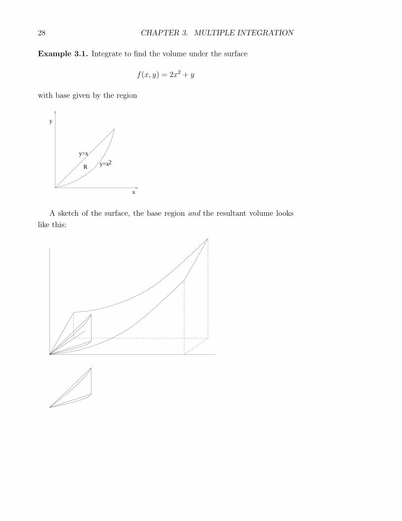
Example 3.1. Integrate to find the volume under the surface
f(x, y) = 2x2 + y
with base given by the region
R
y=x
y=x2
x
y
A sketch of the surface, the base region and the resultant volume looks
like this:

3.2. MULTIPLE INTEGRATION 29
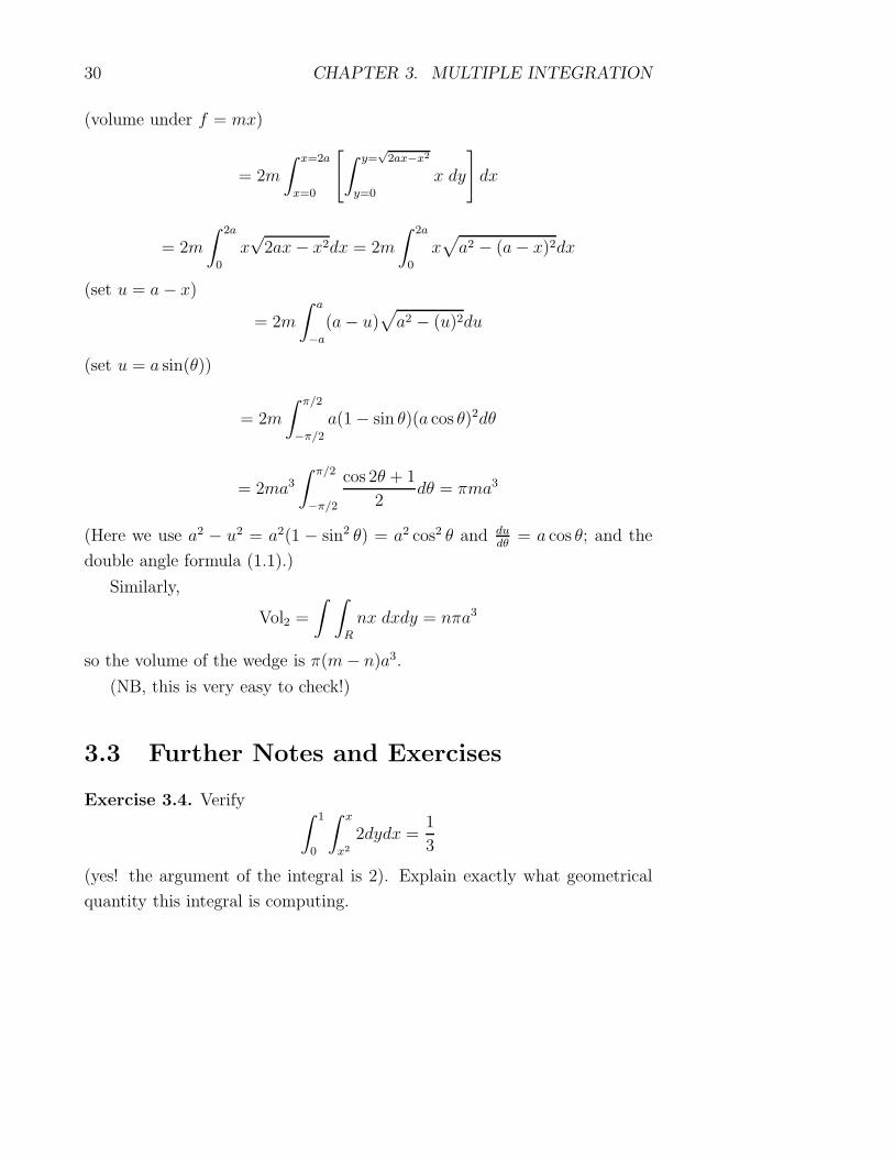
(Here at the bottom we have extracted a little sketch of the volume on
its own, as a guide to the eye.)
The integral is
I =
∫∫
R
(2x2 + y)dxdy
Basic idea:
I =
∫ x=1
x=0
[∫ y=x
y=x2
(2x2 + y)dy
]
dx
In the part in square brackets we regard x as constant (!) — then we can do
the integral (but the answer will depend on x):
I =
∫ x=1
x=0
F (x)dx
where
F =
∫ y=x
y=x2
(2x2 + y)dy = [2x2y +y2
2]y=xy=x2
= 2x3 +x2
2− 2x4 − x4
2so
I =
∫ 1
0
(2x3 +x2
2− 5x4
2)dx
=
[2x4
4+
x3
6− 5
2
x5
5
]1
0
=1
2+
1
6− 1
2=
1
6
Exercise 3.2. Compute the same integral, but performing the∫
dx first.
(Hint: the main problem is to correctly give the limits.)
Example 3.3. Consider the cylinder (tube) in 3d given by
x2 + y2 = 2ax (a a constant)
Consider further that we cut through this tube in 2 planes: z = mx and
z = nx (m, n constants).
Find the volume of the resultant wedge.
Idea: Volume = Volume1 - Volume2 where
Vol1 =
∫ ∫
R
mx dxdy
30 CHAPTER 3. MULTIPLE INTEGRATION
(volume under f = mx)
= 2m
∫ x=2a
x=0
[∫ y=
√2ax−x2
y=0
x dy
]
dx
= 2m
∫ 2a
0
x√
2ax − x2dx = 2m
∫ 2a
0
x√
a2 − (a − x)2dx
(set u = a − x)
= 2m
∫ a
−a
(a − u)√
a2 − (u)2du
(set u = a sin(θ))
= 2m
∫ π/2
−π/2
a(1 − sin θ)(a cos θ)2dθ
= 2ma3
∫ π/2
−π/2
cos 2θ + 1
2dθ = πma3
(Here we use a2 − u2 = a2(1 − sin2 θ) = a2 cos2 θ and dudθ
= a cos θ; and the
double angle formula (1.1).)
Similarly,
Vol2 =
∫ ∫
R
nx dxdy = nπa3
so the volume of the wedge is π(m − n)a3.
(NB, this is very easy to check!)
3.3 Further Notes and Exercises
Exercise 3.4. Verify∫ 1
0
∫ x
x2
2dydx =1
3
(yes! the argument of the integral is 2). Explain exactly what geometrical
quantity this integral is computing.
3.3. FURTHER NOTES AND EXERCISES 31
Exercise 3.5. Verify
∫ 2
1
∫ 3y
y
(x + y)
9dxdy =
14
9
Explain exactly what geometrical quantity this integral is computing.
Exercise 3.6. Verify
∫ 2
−1
∫ x(x+1)
2(x+1)(x−1)
x
2dydx =
9
8
Explain exactly what geometrical quantity this integral is computing.
Exercise 3.7. A cylindrical well is bored vertically down into the New
Mexico desert, with interior sectional radius 3m. The well wall is made of a
relatively thin layer of concrete.
A cylindrical tunnel is bored horizontally under the desert, again with
interior sectional radius 3m, by a separate Engineering company, but follow-
ing a similar construction method. Unfortunately the central axes of the two
tubes coincide at one point under the desert! What is the volume of the
region common to these two tubes.
(HINT: Set up a coordinate system with the y and z axes being the axes of
the two tubes. Then they can meet at (0, 0, 0) say. You could draw a picture
of this situation. Now construct a suitable double integral by considering the
equations describing the shapes of the two tubes.)

32 CHAPTER 3. MULTIPLE INTEGRATION
2003 COURSEWORK 1: Do exercises 2.13, 2.14, 2.16,
2.17, and 3.7.
You must read the separate sheet of advice and rules for coursework submis-
sion. The rules are binding on any submission.
3.4 Polar coordinates
In ordinary integration, we are familiar with the method of change of vari-
ables (we just used it several times above!). There is a multiple integral
generalisation which can be just as useful.
We begin with an example. Recall:
(x,y)
r
x
y
θ
That is, x = r cos θ, y = r sin θ.
The approximate area of the shaded region in
x
y
θ
∆ r
∆θ

3.4. POLAR COORDINATES 33
is r∆r∆θ.
Thus we can make a change of variables in a double integral (correspond-
ing to moving from the Cartesian to the polar coordinate system) as follows:
I =
∫∫
R
f(x, y)dxdy =
∫∫
R
f(r cos θ, r sin θ)rdrdθ
(Note the ‘extra’ r!)
To see the point of this we need an example.
Example 3.8.
I =
∫∫
R
1 −√
x2 + y2dxdy
where the region R is the disk bounded by the unit circle.
I =
∫ 2π
0
∫ 1
0
(1 − r)rdrdθ
=
∫ 2π
0
[r2
2− r3
3
]1
0
dθ = 2π1
6=
π
3.
Example 3.9. The integral
I =
∫ ∞
0
exp(−x2)dx
is a very important (Gaussian) and difficult single integral. (Sketch the curve
of the argument, and recall the role of this function in, for example Statistics,
to see why it is so important.)
I2 = I.I =
(∫ ∞
0
exp(−x2)dx
)(∫ ∞
0
exp(−y2)dy
)
=
∫ ∞
0
∫ ∞
0
exp(−x2 − y2)dxdy =
∫ ∫
R
exp(−x2 − y2)dxdy
=
∫ ∫
R
exp(−r2)rdrdθ =
∫ π/2
0
[∫ ∞
0
exp(−r2)rdr
]
dθ
(We are doing an improper integral here. The answer we will get is correct,
but to be more careful we could have considered
I = lima→∞
∫ a
0
e−x2
dx

34 CHAPTER 3. MULTIPLE INTEGRATION
for which the change of variables is slightly harder to implement.) So
I2 =
∫ π/2
0
[
−1
2exp(−r2)
]∞
0
dθ =π
4.
So I =√
π2
.
3.5 General change of variables
Just as
x = r cos θ = x(r, θ)
y = y(r, θ) = r sin θ
we could have x = x(u, v), y = y(u, v). Then
∫ ∫
R
f(x, y)dxdy =
∫ ∫
R
f(x(u, v), y(u, v)) |D| dudv
where D is the JACOBIAN:
D =
(∂x∂u
∂x∂v
∂y∂u
∂y∂v
)
.
This generalises the single change of variables∫
f(x)dx =
∫
f(x(u))dx
dudu.
Example 3.10. x = r cos θ, y = r sin θ
|D| = r cos2 θ + r sin2 θ = r
as we argued explicitly earlier!
Exercise 3.11. Compute
I =
∫ ∫
R
√
1 − (x2 + y2)dxdy
where R is the interior of the unit disk. Interpret your answer geometrically.

3.6. SPHERICAL POLAR COORDINATES 35
I =
∫ 2π
0
∫ 1
0
√1 − r2 rdrdθ
Substituting r = sin φ we get
I =
∫ 2π
0
∫ π2
0
cos φ sin φ cos φ dφdθ.
Now
cos φ sin φ cos φ = sin φ − sin3 φ =1
4(sin 3φ + sin φ)
(hint: compute sin3 φ = ( eiφ−e−iφ
2i)3). So
I =
∫ 2π
0
[1
4(− cos 3φ
3− cos φ)
]π2
0
dθ =2π
3.
3.6 Spherical polar coordinates
Spherical polar coordinates are the generalisation of polar coordinates to
three dimensions. We have (x, y, z) → (r, θ, φ) as follows.
x
y
z
(x,y,z)
r
φ
θ
36 CHAPTER 3. MULTIPLE INTEGRATION
That is
x = r cos φ sin θ
y = r sin φ sin θ
z = r cos θ
so the Jacobian is
D =
∣∣∣∣∣∣∣
∂x∂r
∂x∂θ
∂x∂φ
∂y∂r
∂y∂θ
∂y∂φ
∂z∂r
∂z∂θ
∂z∂φ
∣∣∣∣∣∣∣
=
∣∣∣∣∣∣∣
cos φ sin θ r cos φ cos θ . . .
sin φ sin θ ∂y∂θ
∂y∂φ
cos θ −r sin θ 0
∣∣∣∣∣∣∣
= r2 sin θ.
Example 3.12. A solid object S has density δ(x, y, z). Then it has mass
m(S) =
∫ ∫ ∫
S
δ(x, y, z) dxdydz. (3.1)
Consider a hemispherical object with density
δ = 17√
(x − xc)2 + (y − yc)2 + (z − zc)2 Kg m−3,
where (xc, yc, zc) is the centre of the corresponding full sphere. What is its
mass?
m(S) =
∫ 2π
0
∫ π2
0
∫ a
0
17r(r2 sin θ)drdθdφ
= 17
∫ 2π
0
∫ π2
0
a4
4sin θ dθdφ =
17a4
4
∫ 2π
0
[− cos θ]π2
0 dφ =17πa4
2.
The CENTRE OF MASS of S is (x, y, z) where
x =
∫ ∫ ∫
Sx δ(x, y, z) dxdydz
m(S)
y =
∫ ∫ ∫
Sy δ(x, y, z) dxdydz
m(S)

3.7. EXAMPLES AND EXERCISES 37
z =
∫ ∫ ∫
Sz δ(x, y, z) dxdydz
m(S)
Exercise 3.13. Compute the CoM of our hemisphere. I.e.
x =
∫ ∫ ∫
Sr cos φ sin θ (17r)r2 sin θ drdθdφ
m(S)= 0 = y
z =
∫ ∫ ∫
Sr cos θ (17r)r2 sin θ drdθdφ
m(S)
=
∫ 2π
0
∫ π2
0
∫ a
0r cos θ (17r)r2 sin θ drdθdφ
m(S)
=2
πa4
a5
52π
∫ π2
0
cos θ sin θ dθ =4
5a
[sin2 θ
2
]π2
0
=2a
5
Thus the CoM is (0, 0, 2a5).
Is this realistic??!!
3.7 Examples and Exercises
3.7.1 Actuarial Science, Quantity and Physics
This section is not examinable. It is here to provide an intuitive and appli-
cable context for problems in integration.
Recall the following facts from elementary Newtonian mechanics. 1 If
you push an object along a line through its centre of mass you will accelerate
it. For a given force applied F , the acceleration a is inversely proportional
to the mass m of the object:
F = ma = mdv
dt= m
d2x
dt2=
dM
dt
1See any standard Physics or Engineering text, for example. (One such is W. Wilson’s
Theoretical Physics (Methuen).)
38 CHAPTER 3. MULTIPLE INTEGRATION
where t is time, v is velocity, x is distance and M = mv is momentum, all in
appropriate units.
If you accelerate the object over some distance, raising its velocity, you
have put energy into it. This movement energy is called kinetic energy. The
total kinetic energy an object has (relative to some coordinate system in
which velocity is measured) is given by
E =1
2mv2 =
1
2Mv
in appropriate units.
Now suppose that our object and forces applied to it ‘live’ in two dimen-
sions rather than one. There is an equation of motion for each direction.
Suppose for definiteness that the force F acts along the line between the ob-
ject and the centre of coordinates (i.e. this is how we choose our coordinate
frame — which we are free to do); and let (x1, x2) be the coordinates of our
object. We can resolve the force into x1 and x2 components by elementary
trigonometry:
md2xi
dt2= F
xi√
x21 + x2
2
(i = 1, 2)
Considering the combination of these equations x2(i = 1) − x1(i = 2) we
haved(Ω = m(x1x
′2 − x2x
′1))
dt= 0
that is, Ω is constant in this situation. This Ω is called the angular momentum
of the object. It is the angular equivalent of the ordinary momentum mv. As
we have seen, it is not changed by a radial force. It is changed by a tangential
force.
If our object is moving with velocity v at an angle θ to the radial line
from the centre to the object, then its velocity component in the tangential
direction is v sin(θ) (elementary trigonometry) and its angular velocity is the
analogue of ordinary velocity defined by
ω =v sin(θ)
r
3.7. EXAMPLES AND EXERCISES 39
where r is the distance from the origin. The angular momentum is propor-
tional to the mass times the angular velocity:
Ω = mr2ω
This is the same as for ordinary momentum (except for the factor r2 which
allows for the fact that, for a given angular velocity, the further away from
the origin we are the greater the ‘linear’ velocity).
Now consider an object in the xy plane rotating about a fixed axis (for
simplicity let us make it the z-axis). If φ measures the angle made by the
line from the object to the origin and the x-axis, then
v = rdφ
dt
so the kinetic energy is
1
2mv2 =
1
2mr2
(dφ
dt
)2
Now suppose we have a rigid object made up of many particles (m1,
m2, ..., say), again rotating about the fixed axis. Since it is rigid, all the
particles have the same angular velocity. The total kinetic energy, the sum
of individual energies computed above, is thus
T =1
2
(∑
i
mir2i
)(dφ
dt
)2
The quantity (∑
i mir2i ) is the moment of inertia of the composite object
with respect to the given axis. It plays the same role in rotating motion
as the mass does in the expression (1/2)mv2 for the kinetic energy in linear
motion.
By considering a solid object as the limit of a collection of tiny individual
chunks we can reduce the computation of its moment of inertia to an integral.
Suppose that ρ(x, y, z) gives the density per unit volume, and that the object

40 CHAPTER 3. MULTIPLE INTEGRATION
occupies a volume of shape V . Since the distance from the z-axis is r2 =
x2 + y2 we have
Iz =
∫ ∫ ∫
V
ρ(x, y, z)(x2 + y2) dx dy dz
where Iz denotes that this is the moment with respect to the z-axis. (This
generalises in a natural way to rotation about an arbitrary axis, but this need
not concern us here.)
3.7.2 Integration related examples
A straight line in the xy plane partitions the plane into two parts (y = 0
partitions the plane into a region above the line and a region below the
line, for example). A curved line without an endpoint (i.e. either closed or
infinite) partitions the plane similarly.
Sets of curves will further partition the plane into subregions. For exam-
ple, three straight lines, none of which are parallel, will partition the plane
into a number of regions. Most of these regions are infinite in extent (‘un-
bounded’), but one is finite — a triangle (unless all three lines intersect at
the same point!). In such a case we say the finite region is bounded by the set
of lines. Generalising from this: even if the set of lines is curved, provided
that precisely one part of the partition of the plane they describe is finite,
we call this the region bounded by the curves.
Exercise 3.14. Sketch the region of the xy plane bounded by each of the
following sets of curves:
x2 + y2 = 16;
x = y, x = 2, y = 3;
x = 1, x = 2, y = 3, y = 6;
y = sin(x) (0 ≤ x ≤ π/3), x = π/3, y = 0.
Express the area of the region as a double integral (or multiple thereof) in
each case. Evaluate this double integral.
Exercise 3.15. Sketch the volume bounded by x = 0, y = 0, z = 6,
z = x + y. Compute this volume by means of a double integral. (Ans=36)
3.7. EXAMPLES AND EXERCISES 41
Exercise 3.16. Sketch and Evaluate:∫ a
0
∫ a−x
01 dy dx;
∫ 1
0
∫ x1/2
xxy2 dy dx;
∫ a
0
∫ x
0(x2 + y2)dy dx;
∫ π/2
−π/2
∫ 2a cos(θ)
0r2 cos(θ) dr dθ.
(Ans=a2/2; 1/35; a4/3; πa3)
Exercise 3.17. A new design of motorised food slicer blade (or helocopter
rotor, take your pick!) has shape given by the region R of the x1x2-plane
bounded by the curves x21 = x2, x2 = 1, x1 = 2. It has uniform thickness and
density in this region (and has unit mass per unit area). Sketch the shape of
the slicer blade. Work out the moment of inertia with respect to the x3-axis:∫ ∫
R
(x21 + x2
2) dx1 dx2
(Ans=1006/105)
Exercise 3.18. Formulate and compute a double integral which determines
the volume of a sphere.
Formulate and compute a triple integral which determines the volume of a
sphere.
Exercise 3.19. Recall that the region of integration of the double integral
I1 =
∫ 1
0
(∫ 1
0
3 dy
)
dx
is the square in the (x, y) plane with corners (0,0),(1,0),(1,1),(0,1). Sketch
this region. What is the value of I1? (Hint: you do not need to do an
integral!)
Exercise 3.20. Sketch the region of integration in the double integral
I =
∫ 1
0
(∫ 1
√x
sin
(y3 + 1
2
)
dy
)
dx.
Re–express I with the x–integral as the inner (first) integral. By thus chang-
ing the order of integration, evaluate I. (Hint: you will need to make at least
one change of variables.)
42 CHAPTER 3. MULTIPLE INTEGRATION
Exercise 3.21. Show that in polar coordinates the equation of the circle
(x − 1)2 + y2 = 1 takes the form
r = 2 cos θ,
where −π2≤ θ ≤ π
2.
Hence, by using the cylindrical coordinate system (r, θ, z) or otherwise,
find the volume of the solid enclosed in the vertical cylinder (x−1)2 +y2 = 1
bounded below by the plane z = 0 and bounded above by the cone z =
2 −√
x2 + y2.

Chapter 4
Differential Equations
Examples:
df(x)
dx= 3 (4.1)
d2f(x)
dx2= 6x (4.2)
d2f(x)
dx2+ 7
df(x)
dx= (f(x))2 + 7 loge(x) (4.3)
Solution: Find a function f(x) such that the Differential Equation (DE) is a
true identity. E.g.
(4.1) f(x) = 3x + 7
(4.2) f(x) = x3 + πx − 4
(4.3) ?!
A DE is linear if it can be expressed in the form
P (D) f(x) = q(x)
where D is the “differential operator” ddx
(which is only meaningful when
acting on a f(x) on its right!) and P (D) is a polynomial; and q(x) is a given
function.
Example 4.1.d2f
dx2+ 7x
df
dx− 2f = sin x
43

44 CHAPTER 4. DIFFERENTIAL EQUATIONS
= (D2 + 7xD − 2)f = sin x
If the coefficients in P are constants it is a CONSTANT COEFFICIENT
LINEAR DE. The order of P is the ORDER of the DE. For example,
(D3 − 7D + 3)f(x) = tanx
is a third order linear constant coefficient DE.
Exercise 4.2. Find a 2nd order linear DE for which f(x) = e3x is a solution.
In general, solving DEs is HARD. So, in general, we use guesswork and
standard recipes to find solutions. Here we will look at many such recipes.
4.1 Solutions I
1. Ifdf
dx= q(x)
f =
∫df
dxdx =
∫
q(x)dx + c
(note the constant of integration c).
2. Ifdf
dx= 7f
∫df
f=
∫
7dx
“separation of variables”, giving
loge f = 7x + c
so f = ece7x = Ce7x where C is a constant.
DEs may have multiple possible solutions in general (or none!). For eachddx
we can (think of) undoing it with an∫−dx. Each such integration has
an integration constant, so a DE of order n has n undetermined constants in
its general solution. That is, n constants which can be determined freely to
obtain a specific solution.
4.1. SOLUTIONS I 45
DEs often appear like this:
Solved2f
dx2+ 3
df
dx= 2x
subject to f(0) = 0, f ′(0) = 7. These x = 0 conditions are called INITIAL
CONDITIONS. Using them (if there are enough) we can fix the constants of
integration.
4.1.1 Homogeneous Linear DEs
A linear DE of form
P (D)f(x) = 0 (4.4)
is called HOMOGENEOUS.
Proposition 4.3. Suppose f1(x), f2(x) are specific given solutions to (4.4).
(This means that P (D)f1(x) = 0 and P (D)f2(x) = 0 are true identities.)
Then A1f1(x) + A2f2(x) is also a solution for any constants A1, A2.
This is the miracle of LINEARITY.
Proof:
P (D)(A1f1(x) + A2f2(x)) = A1P (D)f1(x) + A2P (D)f2(x) = 0 + 0 = 0.
Done.
Example 4.4. (D − 3)(D − 4)f(x) = 0
Trial form of solution:
f(x) = eλx
Now,
Deλx =deλx
dx= λeλx
so substitution gives
(λ − 3)(λ − 4)eλx = 0.
This is true for all x only when λ = 3 or 4, so f1(x) = e3x and f2(x) = e4x
are both solutions.
Exercise 4.5. So is 7e3x + 21πe4x. Confirm.

46 CHAPTER 4. DIFFERENTIAL EQUATIONS
More generally, suppose
n∏
i=1
(D − λi)f(x) = 0
where the product is the factored form of P (D). Then
f(x) =∑
i
Aieλix
is the general solution.
(Note
Proposition 4.6. Every complex polynomial may be factorised with linear
factors over the complex numbers.
so we can ALWAYS solve constant coefficient P (D)f = 0 in this way.)
Example 4.7.d2f
dx2= −9f
(D2 + 9)f = 0 = (D + 3i)(D − 3i)
so
f = A1e3ix + A2e
−3ix.
Note as usual thate3ix + e−3ix
2= cos 3x
e3ix − e−3ix
2i= sin 3x
so
f = C cos 3x + D sin 3x
is an equally good way of writing the answer.
Note here that 2nd order DE, implies 2 undetermined constants in the
general solution.
Overall, solving an nth order linear homogeneous constant coefficient DE
requires only to find the roots of the associated P (D).

4.1. SOLUTIONS I 47
The polynomial equation P (m) = 0 is sometimes called the auxilliary
equation (the dummy variable name m here has just been chosen to avoid
confusion with commonly used variable names, already possibly occuring in
the problem).
4.1.2 Inhomogeneous DEs
P (D)f(x) = q(x) 6= 0 (4.5)
where q(x) is given.
We break the problem of finding the general solution into 2 parts:
1. find any single solution by guesswork (!) (called the particular solution
fP );
2. find the general solution to P (D)f(x) = 0 (called the associated homoge-
neous DE) as above. (NB, we again refer to the corresponding polynomial
equation as the auxilliary equation.)
The general solution to the associated homogeneous DE is called the
Complementary Function fCF .
Proposition 4.8. The general solution to (4.5) is the sum of these.
Proof: Exercise.
Example 4.9.df
dx− 3f = 7x2 + 3x
Looking at the form of the RHS, we guess that f(x) a polynomial might
be a solution. Try it! . . .
More Clues:
If the RHS looks like aebx then try
fP = Axkebx
where k is such that the auxilliary equation has m = b as a root of multiplicity
k.
If the RHS looks like a sin(bx) then try
fP = xk(A sin(bx) + B cos(bx))
48 CHAPTER 4. DIFFERENTIAL EQUATIONS
where k is such that the auxilliary equation has m2 + b2 as a real quadratic
factor of multiplicity k.
Example 4.10.d2y
dx2− 3
dy
dx+ 2y = e2x
The auxilliary equation is m2 −3m+2 = 0, so m = 1, 2, so try a solution
of form
Y (x) = Axe2x
Substituting in gives
A(x4e2x + 2.2e2x − 3x2e2x − 3e2x + 2xe2x) = e2x
so that A = 1. Thus the general solution is
y = Cex + De2x + xe2x
where C, D are arbitrary constants.
Example 4.11.d2y
dx2+ 4y = 3 sin 2x
m2 + 4 = 0
so try
Y (x) = x(A sin 2x + B cos 2x).
Substitute into the DE to get
Y = −3
4x cos 2x
then
y = Ce2ix + De−2ix − 3
4x cos 2x = E cos 2x + F sin 2x − 3
4x cos 2x.
Exercise 4.12.
d3y
dx3− 2
d2y
dx2− dy
dx+ 2y = 6x + sin x

4.2. WRONSKIANS, VARIATION ETC. 49
1
4.2 Wronskians, Variation etc.
Consider
a0d2y
dx2+ a1
dy
dx+ a2y = f(x) (4.6)
(f(x) given), with Complementary Function (CF)
y = A1y1 + A2y2
(A1, A2 constants). Now try to find
Y = v1(x)y1 + v2(x)y2
a solution of (4.6), given that
v′1y1 + v′
2y2 = 0 (4.7)
(so thatdY
dx= v1y
′1 + v2y
′2
d2Y
dx2= v1y
′′1 + v2y
′′2 + v′
1y′1 + v′
2y′2
etc.). Substituting into (4.6):
v′1y
′1 + v′
2y′2 =
f(x)
a0
so from (4.7) we have
v′1 =
−y2f
a0(y1y′2 − y′
1y2)
1Answer for Particular solution:
Y (x) = 3(x +1
2) +
1
10(2 sinx + cosx).
50 CHAPTER 4. DIFFERENTIAL EQUATIONS
(y1y′2 − y′
1y2 is called the WRONSKIAN)
v′2 =
y1f
a0(y1y′2 − y′
1y2)
so
v1 = − 1
a0
∫y2f
y1y′2 − y′
1y2
dx
and v2 similarly. Thus the general solution to (4.6) is
y = (A1 + v1)y1 + (A2 + v2)y2.
Example 4.13.d2y
dx2− y = ex
CF: y1 = ex, y2 = e−x
Y (x) = v1ex + v2e
−x
where
v1 = −∫
e−xex
−exe−x − exe−xdx = x/2
v2 = . . . = −−e2x
4.
Thus the general solution is
y = (A1 +x
2)ex + (A2 −
e2x
4)e−x
4.3 General linear second order equations
d2y
dx2+ p(x)
dy
dx+ q(x)y = f(x)
with p, q, f given, CANNOT always be solved!
Sometimes it can be . . . E.g. by substitution, or by knowing one solution
already (somehow!).

4.3. GENERAL LINEAR SECOND ORDER EQUATIONS 51
Example 4.14. Suppose y = v(x) IS a solution of
xd2y
dx2+
dy
dx+ xy = 0.
A second solution can be found by putting
y = u(x)v(x)
and solving for u(x). This gives
1
w
dw
dx+
2
v
dv
dx+
1
x= 0
(w = dudx
), sodu
dx=
A
xv2
(by integration, with A the integration constant) and
u(x) = A
∫dx
xv2+ B
so
y = Av
∫dx
xv2+ Bv.
In particular, consider
Example 4.15.
x2 d2y
dx2− x(x + 2)
dy
dx+ (x + 2)y = 0
One solution, note, is y1 = x. So, try y2 = xu(x). Substituting:
d2u
dx2− du
dx= 0
so u = Aex + B and
y = x(Aex + B)
is the general solution.
52 CHAPTER 4. DIFFERENTIAL EQUATIONS
4.4 Series solution methods
Example 4.16. To solve
(1 − x2)d2y
dx2− 5x
dy
dx− 3y = 0 (4.8)
guess a solution of the form
y = y(0) + xy(1)(0) +x2
2!y(2)(0) + . . . +
xr
r!y(r)(0) + . . .
where y(r)(0) = drydyr
∣∣∣x=0
a constant (as before).
This is the MacLaurin Expansion (ME) of an arbitrary differentiable func-
tion y(x). Repeatedly differentiating (4.8) gives
(1 − x2)y(n+2) − x(2n + 5)y(n+1) − (n + 1)(n + 3)y(n) = 0
(exercise!). Substituting our ME in:
y(n+2)(0) = (n + 1)(n + 3)y(n)(0)
(using x = 0).
Hence
y(2)(0) = 1 × 3 × y(0)
y(3)(0) = 2 × 4 × y(1)(0)
y(4)(0) = 3 × 5 × y(2)(0) = 1 × 32 × 5 × y(0)
etc., giving
y = y(0)
(
1 +1.3
2!x2 +
1.32.5
4!x4 + ...
)
+y(1)(0)
(
x +2.4
3!x3 +
2.42.6
5!x5 + ...
)
Note as usual 2 constants undetermined. Fixing these with 2 initial con-
ditions we would have a good (!) approximation to y close to x = 0.
To obtain an approximate solution which is good close to x = a use the
TAYLOR EXPANSION.

4.4. SERIES SOLUTION METHODS 53
Example 4.17. Solve
xd2y
dx2+ (1 + x)
dy
dx+ 2y = 0 (4.9)
near x = 0.
Differentiate n times:
xy(n+2) + (1 + n + x)y(n+1) + (n + 2)y(n) = 0
taking x = 0:
y(n+1)(0) = −n + 2
n + 1y(n)(0).
Thus the coefficients y(r)(0) in the ME are:
y(1)(0) = −2y(0)
y(2)(0) = −3
2y(1)(0) = 3y(0)
y(3)(0) = −4
3y(2)(0) = −4y(0)
y(4)(0) = −5
4y(3)(0) = 5y(0)
so
y = y(0)
(
1 − 2x +3
2!x2 − 4
3!x3 +
5
4!x4 + . . . + (−1)r r + 1
r!xr + . . .
)
(y(0) arbitrary).
NB, only one arbitrary constant, so this is not the general solution. Fol-
lowing our previous notes we may call this solution y1 and try y2 = u(x)y1
in (4.9).
Exercise 4.18. Solve for u(x).
Answer:
u = c
∫e−x
xy21
dx.

54 CHAPTER 4. DIFFERENTIAL EQUATIONS

Chapter 5
Laplace Transforms
Lp[f(x)] =
∫ ∞
0
e−pxf(x) dx
is the Laplace transform of f(x) (x > 0).
IT IS A LINEAR OPERATOR:
Lp[kf(x)] = kLp[f(x)]
Lp[f(x) + g(x)] = Lp[f(x)] + Lp[g(x)]
Simple ones:
Lp[eax] =
∫ ∞
0
e−pxeax dx =1
p − a
(provided p > a).
Lp[xn] =
∫ ∞
0
e−pxxn dx =?
Recall the mnemonic for integration by parts:
duv = udv + vdu
or ∫
udv = uv −∫
vdu.
55

56 CHAPTER 5. LAPLACE TRANSFORMS
In our case we have u = xn and dv = e−px so we get
Lp[xn] =
[xne−px
−p
]∞
0
−∫ ∞
0
e−px
−pnxn−1dx =
n!
pn+1.
Exercise 5.1. Use deMoivre’s theorem etc. to compute Lp[sin ax], Lp[cos ax],
Lp[sinh ax].
“Shift theorem”:
Lp[e−axf(x)] =
∫ ∞
0
e−pxe−axf(x) dx
=
∫ ∞
0
e−(p+a)xf(x) dx = Lp+a[f(x)]
Thus
Lp[e−ax sin(bx)] =
b
(p + a)2 + b2
(p > −a).
5.1 Inverse operator
L−1x [Lp[f(x)]] = f(x)
Again L−1x is linear.
E.g. Since Lp[1] = 1p
L−1x [
1
p] = 1
and L−1x [k
p] = k.
Example 5.2. L−1x
[1
(p+a)(p+b)
]
— use PARTIAL FRACTIONS.
1
(p + a)(p + b)=
A
(p + a)+
B
p + b
implies B = −A = 1a−b
(a 6= b), so
L−1x
[1
(p + a)(p + b)
]
=1
b − a
(e−ax − e−bx
).

5.2. TRANSFORMS OF DIFFERENTIALS 57
Exercise 5.3. Use partial fractions to determine
L−1x
[p
(p2 + a2)(p2 + b2)
]
and
L−1x
[1
p2(p2 + a2)
]
1
Now, what is the point of all this?!
5.2 Transforms of differentials
Lp[dy
dx] =
∫ ∞
0
e−px dy
dxdx =
[ye−px
]∞0
+ p
∫ ∞
0
e−pxydx
= −y(0) + pLp[y]
(assume e−pxy → 0 as x → ∞).
Similarly,
Lp[d2y
dx2] = (exercise)
Lp[dny
dxn] = pnLp[y] − pn−1y(0) − pn−2y(1)(0) − . . . − py(n−2)(0) − y(n−1)(0).
5.3 Solution of Ordinary Differential Equa-
tions
Solve
(D + 2)y = cos x
1Answers:1
b2 − a2(cos ax − cos bx)
x
a2− 1
a3sin ax.

58 CHAPTER 5. LAPLACE TRANSFORMS
given y(0) = 1.
Apply the Laplace transform to both sides:
pLp[y] − y(0) + 2Lp[y] =p
p2 + 1
so
Lp[y] =p
(p + 2)(p2 + 1)+
y(0)
p + 2.
Nowp
(p + 2)(p2 + 1)=
A
p + 2+
Bp + C
p2 + 1
implies A = −B = −2/5, C = 1/5. Thus
Lp[y] =1
5
1
p2 + 1+
2
5
p
p2 + 1+
3
5
1
p + 2.
Now invert the Laplace transform:
y(x) =1
5sin x +
2
5cos x +
3
5e−2x.
Example 5.4. Solve (D2 + a2)y = sin bx.
Laplace:
p2Lp[y] − py(0)− y(1)(0) + a2Lp[y] =b
p2 + b2
so
Lp[y] =b
(p2 + a2)(p2 + b2)+
y(0)
(p2 + a2)+
y(1)(0)
(p2 + a2)
Partial fractions:
Lp[y] =b
b2 − a2
(1
(p2 + a2)− 1
(p2 + b2)
)
+y(0)p
(p2 + a2)+
y(1)(0)
a
a
(p2 + a2)
Invert Laplace:
y(x) =b sin ax
a(b2 − a2)− sin bx
(b2 − a2)+ y(0) cos ax +
y(1)(0)
asin ax.

5.3. SOLUTION OF ORDINARY DIFFERENTIAL EQUATIONS 59
Example 5.5.
(D2 + 2)y(t) − x(t) = 0
(D2 + 2)x(t) − y(t) = 0
Solve simultaneously! for x and y, subject to x(0) = 2, y(0) = 0, x(1)(0) = 0,
y(1)(0) = 0.
First Laplace transform everything:
p2Lp[y] − py(0) − y(1)(0) + 2Lp[y] − Lp[x] = 0
p2Lp[x] − px(0) − x(1)(0) + 2Lp[x] − Lp[y] = 0
Rearranging:
(p2 + 2)Lp[y] − Lp[x] = 0
(p2 + 2)Lp[x] − Lp[y] = 2p
Eliminate, say, Lp[y]:
Lp[x] =2p(p2 + 2)
(p2 + 1)(p2 + 3)
Apply partial fractions method:
x(t) = cos t + cos√
3t
Now eliminate Lp[x] instead:
y(t) = cos t − cos√
3t.
Note that it is relatively easy to check answers by substitution. So, always
check! CHECK NOW!
Exercise 5.6. Verify
Lp[a + bx] =ap + b
p2
Lp[1√x
] =
√π
p.
Exercise 5.7. Solve
(D2 + 4D + 8)y = cos 2x
given y(0) = 2, dydx
∣∣x=0
= 1, using Laplace transforms. (And check your
answer!)

60 CHAPTER 5. LAPLACE TRANSFORMS

Chapter 6
More exercises
Exercise 6.1. This question begins with some revision of Taylor series for
functions of one variable, before going on to investigate the integral of a
function of two variables.
(a) Show that every Taylor series is a Maclaurin series for a certain related
function.
(b) For g(x) a differentiable function, let gi(x) denote the Maclaurin series
for g up to the term in xi.
Recall that the Taylor series for cos(x) about x = 0 (the Maclaurin
series) begins 1 − x2
2+ x4
4!+ . . .. Thus we have the approximation
cos(.1) ∼= 1 − .01
2+
.0001
24+ ... = 1 − .005 + .000004 + ... ∼= .9950
(angles in radians) correct in all four significant figures. Note that each
term in the series contributes in a lower decimal place than the one
before, which makes it clear that the series is convergent.
Using our notation above, if g = cos(x) then g2 = 1 − x2
2. Sketch the
functions g and g2 on the same graph, in the region −.1 < x < .1. Make
a separate sketch showing the functions g and g2 on the same graph, in
the region −1 < x < 1. Comment on the relationships between g and
g2 illustrated by your sketches.
61

62 CHAPTER 6. MORE EXERCISES
(c) Let f(x, y) = cos(x) cos(y). Let f22 denote the Taylor series about
(0, 0) for f up to terms quadratic in x and y (i.e. neglecting cubic, bi-
quadratic, and higher order terms). Determine f22 and hence compute
I1 =
∫ ∫
R
f22dxdy
where R is the square region given by −.1 < x, y < .1. Compute
I2 =
∫ ∫
R
fdxdy
directly for the same region R. Compare and comment on your answers.
Bibliography
[1] G Stephenson, Mathematical Methods for Science Students, 2nd Edition
(Longman, 1973).
[2] M R Spiegel, Theory and Problems of Advanced Calculus, Schaum’s
Outline Series (McGraw Hill, 1988).
63