calculus review
DESCRIPTION
Calculus Review. GLY-4822. Slope. Slope = rise/run = D y/ D x = ( y 2 – y 1 )/( x 2 – x 1 ) Order of points 1 and 2 not critical, but keeping them together is Points may lie in any quadrant: slope will work out - PowerPoint PPT PresentationTRANSCRIPT
Calculus Review
GLY-4822
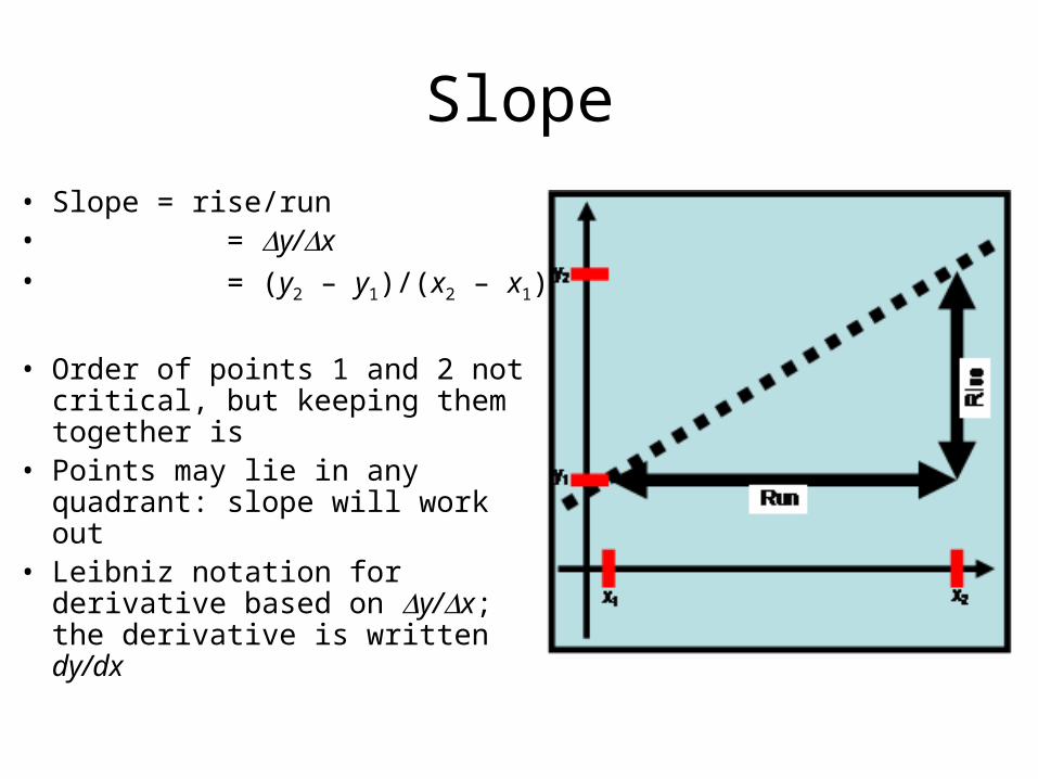
Slope• Slope = rise/run • = y/x • = (y2 – y1)/(x2 – x1)
• Order of points 1 and 2 not critical, but keeping them together is
• Points may lie in any quadrant: slope will work out
• Leibniz notation for derivative based on y/x; the derivative is written dy/dx
Exponents
• x0 = 1
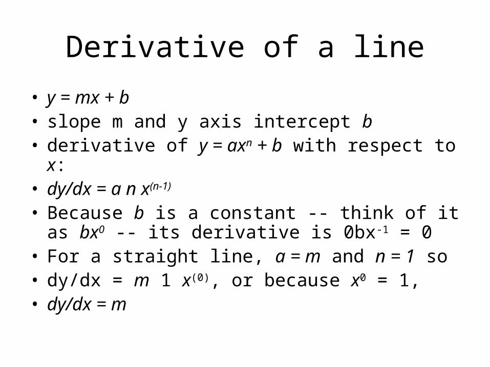
Derivative of a line• y = mx + b• slope m and y axis intercept b• derivative of y = axn + b with respect to x:• dy/dx = a n x(n-1) • Because b is a constant -- think of it as bx0 -- its
derivative is 0bx-1 = 0 • For a straight line, a = m and n = 1 so• dy/dx = m 1 x(0), or because x0 = 1, • dy/dx = m
Derivative of a polynomial
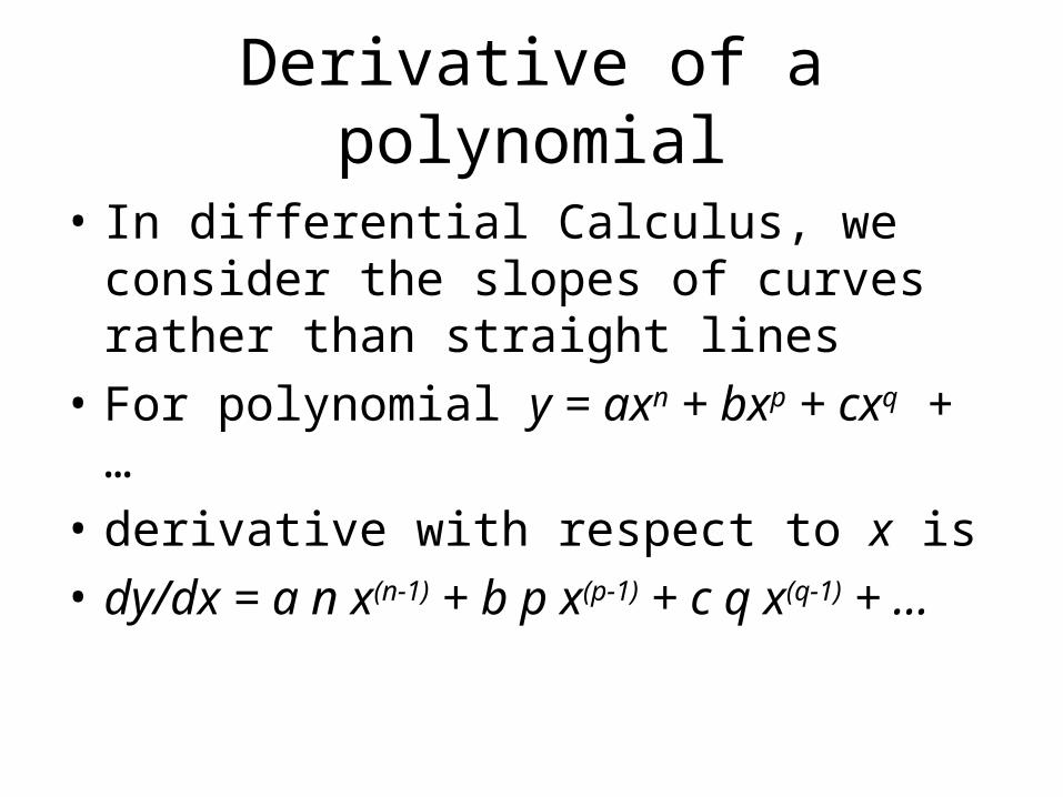
• In differential Calculus, we consider the slopes of curves rather than straight lines
• For polynomial y = axn + bxp + cxq + …• derivative with respect to x is • dy/dx = a n x(n-1) + b p x(p-1) + c q x(q-1) + …
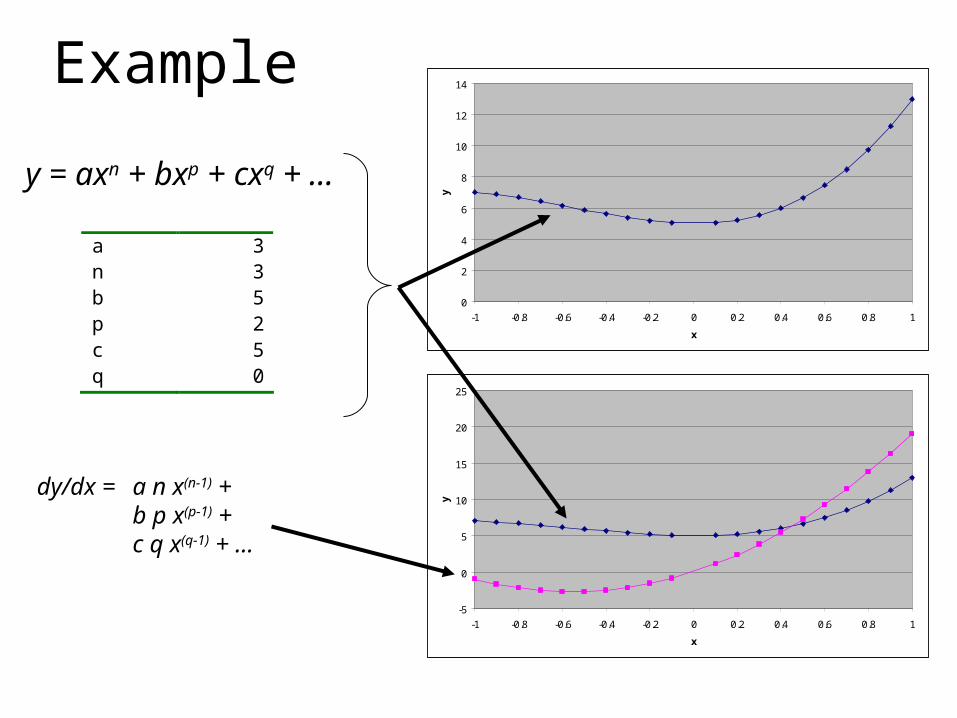
Example
a 3 n 3 b 5 p 2 c 5 q 0
0
2
4
6
8
10
12
14
-1 -0.8 -0.6 -0.4 -0.2 0 0.2 0.4 0.6 0.8 1
x
y
y = axn + bxp + cxq + …
-5
0
5
10
15
20
25
-1 -0.8 -0.6 -0.4 -0.2 0 0.2 0.4 0.6 0.8 1
x
y
dy/dx = a n x(n-1) + b p x(p-1) + c q x(q-1) + …
Numerical Derivatives
• slope between points
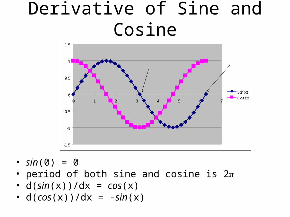
Derivative of Sine and Cosine
• sin(0) = 0 • period of both sine and cosine is 2• d(sin(x))/dx = cos(x) • d(cos(x))/dx = -sin(x)
-1.5
-1
-0.5
0
0.5
1
1.5
0 1 2 3 4 5 6 7
Sin(x)Cos(x)
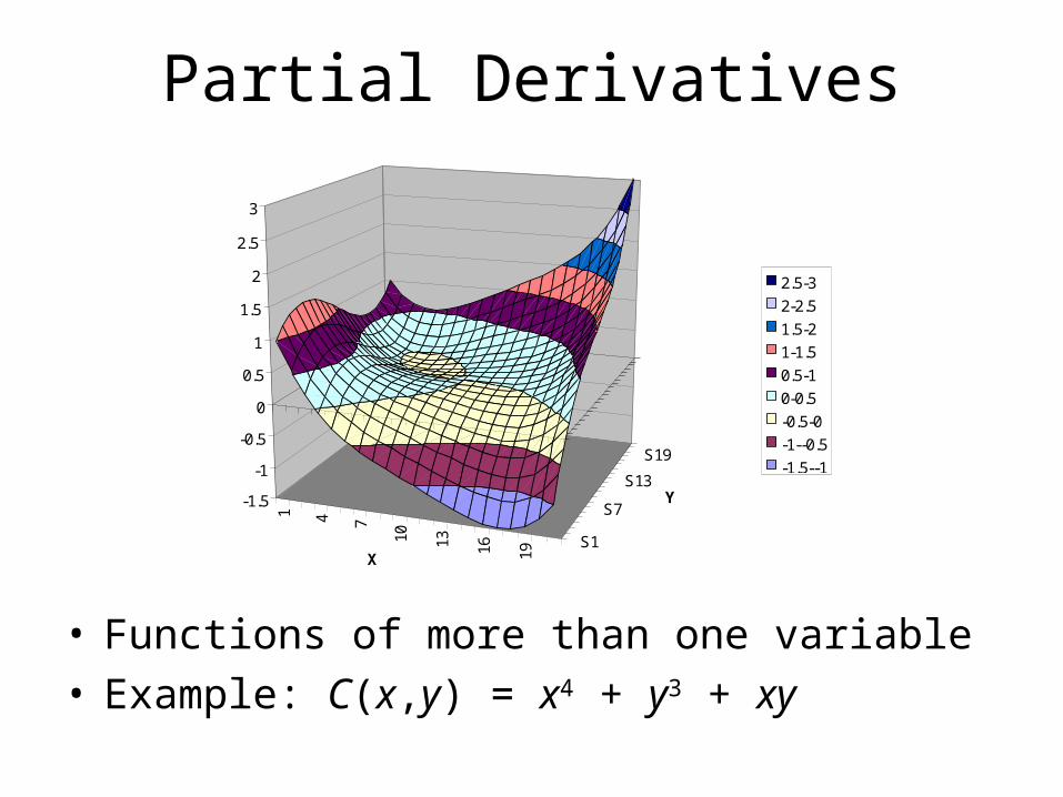
Partial Derivatives
• Functions of more than one variable• Example: C(x,y) = x4 + y3 + xy
1 4 7
10 13 16 19S1
S7
S13
S19
-1.5
-1
-0.5
0
0.5
1
1.5
2
2.5
3
X
Y
2.5-32-2.51.5-21-1.50.5-10-0.5-0.5-0-1--0.5-1.5--1
Partial Derivatives
• Partial derivative of h with respect to x at a y location y0
• Notation h/x|y=y0
• Treat ys as constants• If these constants stand alone, they drop out
of the result• If they are in multiplicative terms involving x,
they are retained as constants
Partial Derivatives
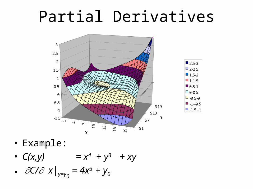
• Example: • C(x,y) = x4 + y3 + xy • C/x|y=y0
= 4x3 + y0
1 4 7
10 13 16 19S1
S7
S13
S19
-1.5
-1
-0.5
0
0.5
1
1.5
2
2.5
3
X
Y
2.5-32-2.51.5-21-1.50.5-10-0.5-0.5-0-1--0.5-1.5--1
WHY?
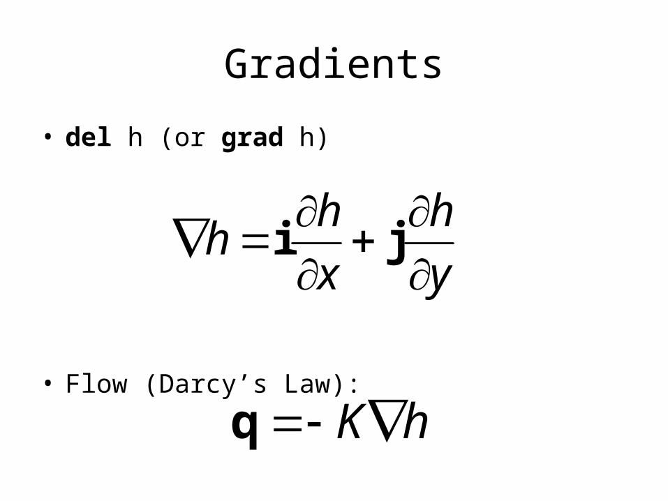
Gradients
• del h (or grad h)
• Flow (Darcy’s Law):
yh
xhh
ji
hKq
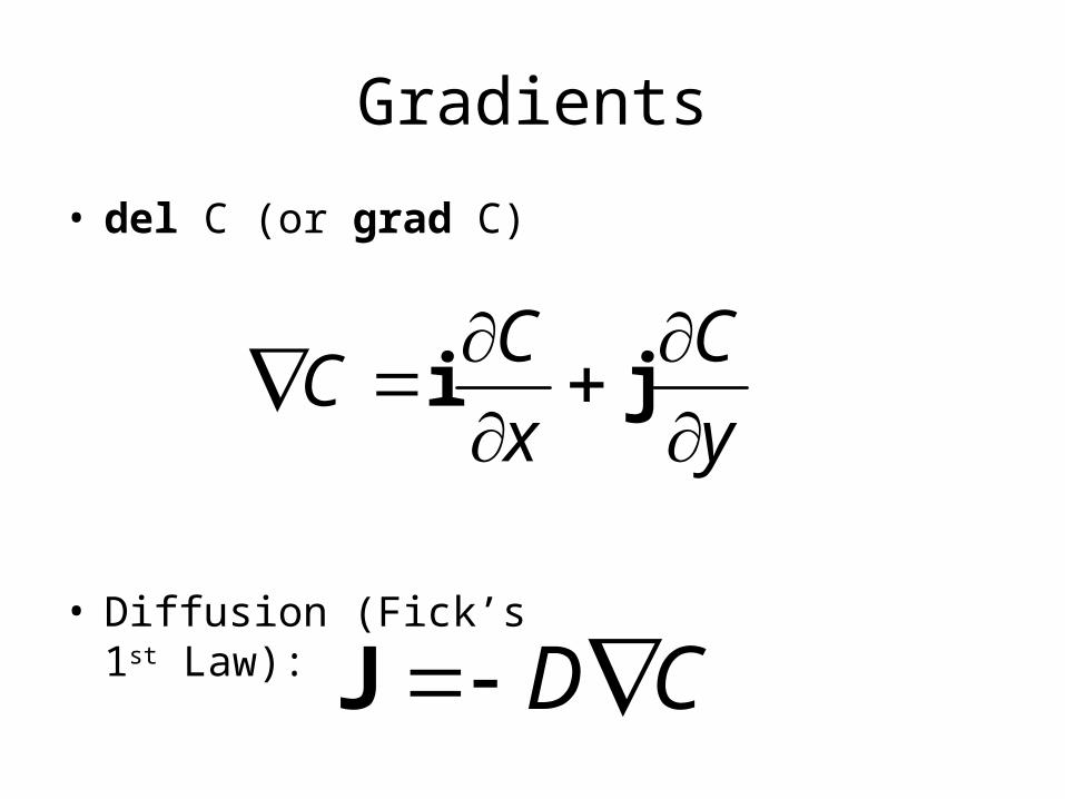
Gradients
• del C (or grad C)
• Diffusion (Fick’s 1st Law):
yC
xCC
ji
CDJ
Basic MATLAB
Matlab
• Programming environment• Post-processer• Graphics• Analytical solution comparisons
• Use File/Preferences/Font to adjust interface font size
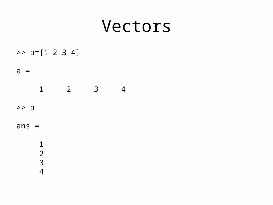
Vectors>> a=[1 2 3 4]
a =
1 2 3 4
>> a'
ans =
1 2 3 4
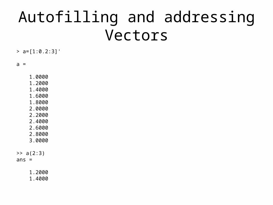
Autofilling and addressing Vectors> a=[1:0.2:3]'
a =
1.0000 1.2000 1.4000 1.6000 1.8000 2.0000 2.2000 2.4000 2.6000 2.8000 3.0000
>> a(2:3)ans =
1.2000 1.4000
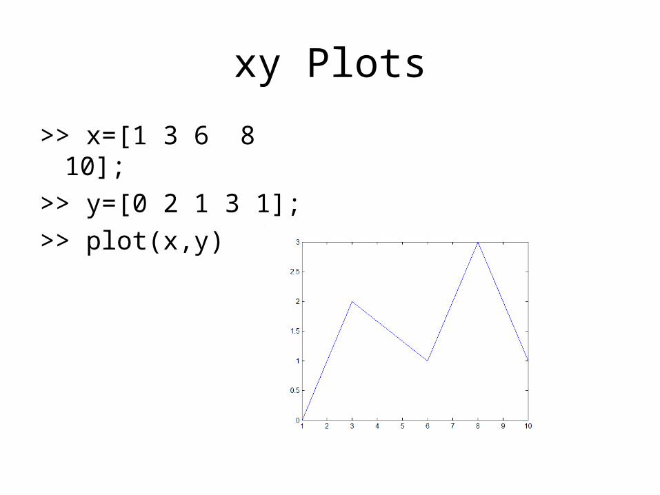
xy Plots
>> x=[1 3 6 8 10];>> y=[0 2 1 3 1];>> plot(x,y)
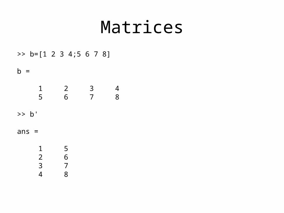
Matrices>> b=[1 2 3 4;5 6 7 8]
b =
1 2 3 4 5 6 7 8
>> b'
ans =
1 5 2 6 3 7 4 8
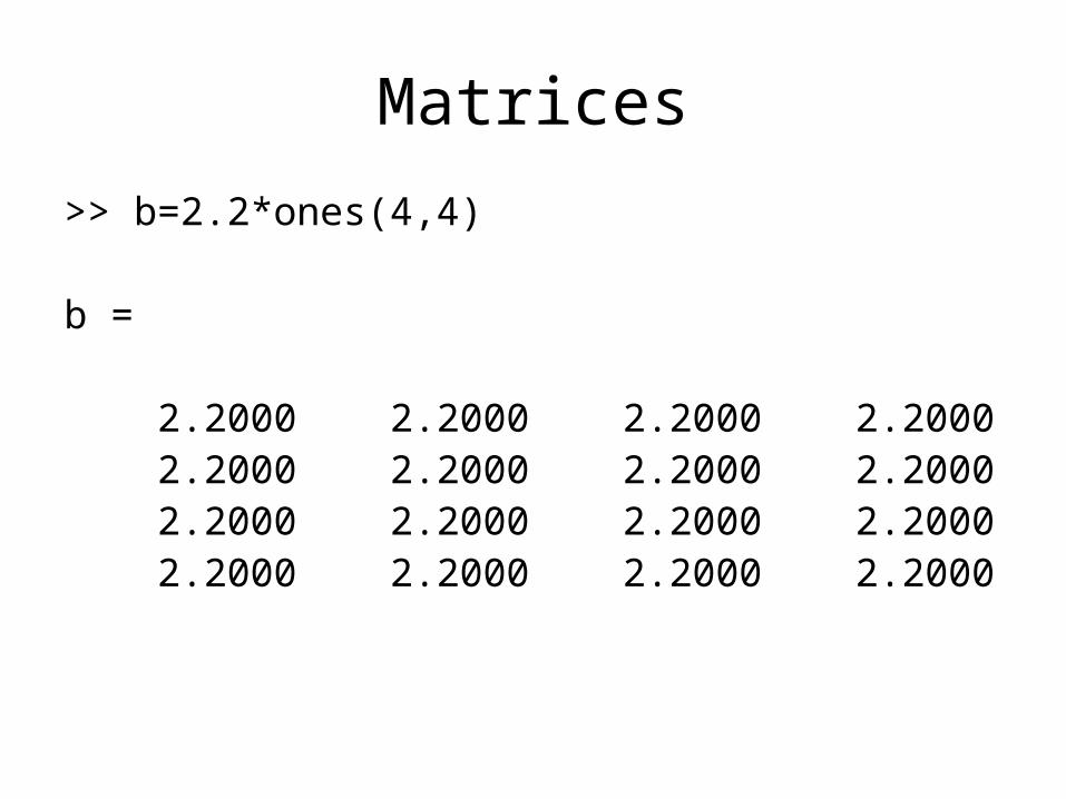
Matrices
>> b=2.2*ones(4,4)
b =
2.2000 2.2000 2.2000 2.2000 2.2000 2.2000 2.2000 2.2000 2.2000 2.2000 2.2000 2.2000 2.2000 2.2000 2.2000 2.2000
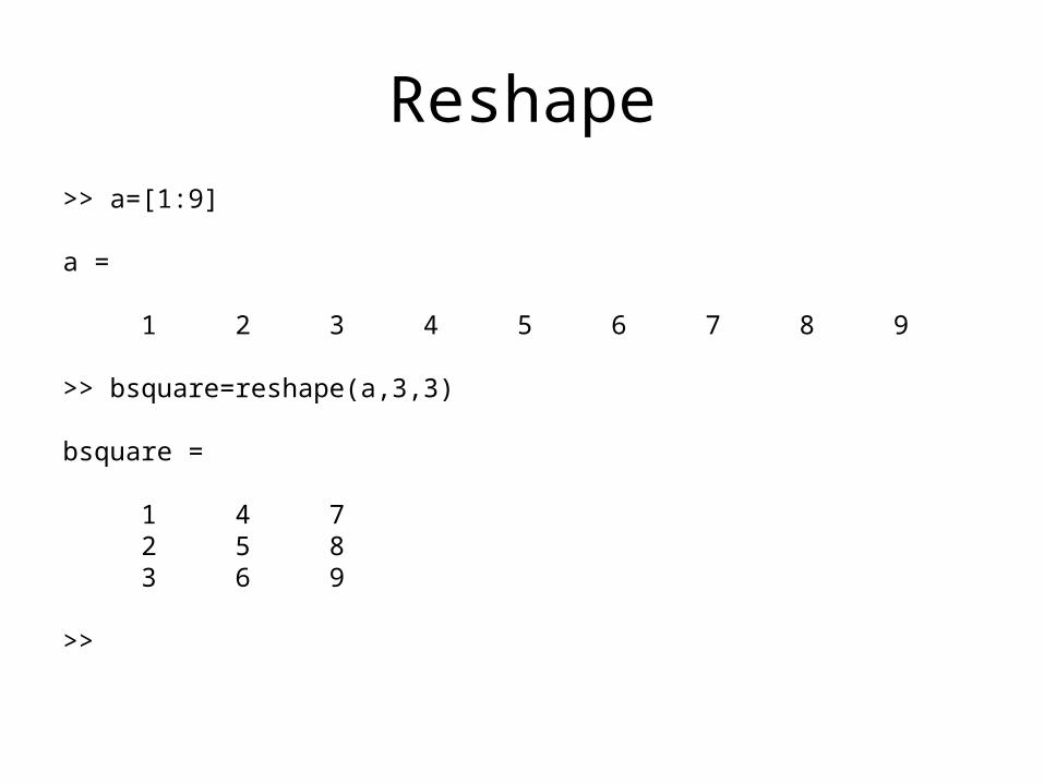
Reshape>> a=[1:9]
a =
1 2 3 4 5 6 7 8 9
>> bsquare=reshape(a,3,3)
bsquare =
1 4 7 2 5 8 3 6 9
>>
Load
• a = load(‘filename’); (semicolon suppresses echo)
If
• if(1)…else…end
For
• for i = 1:10• …• end
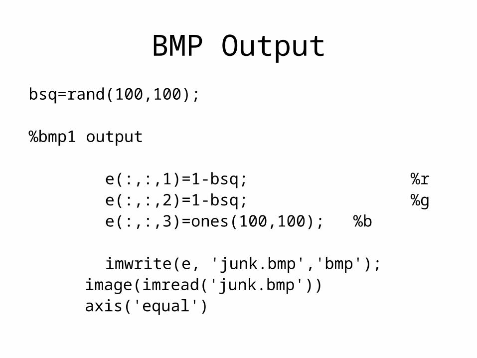
BMP Outputbsq=rand(100,100);
%bmp1 output
e(:,:,1)=1-bsq; %r e(:,:,2)=1-bsq; %g e(:,:,3)=ones(100,100); %b imwrite(e, 'junk.bmp','bmp');
image(imread('junk.bmp')) axis('equal')
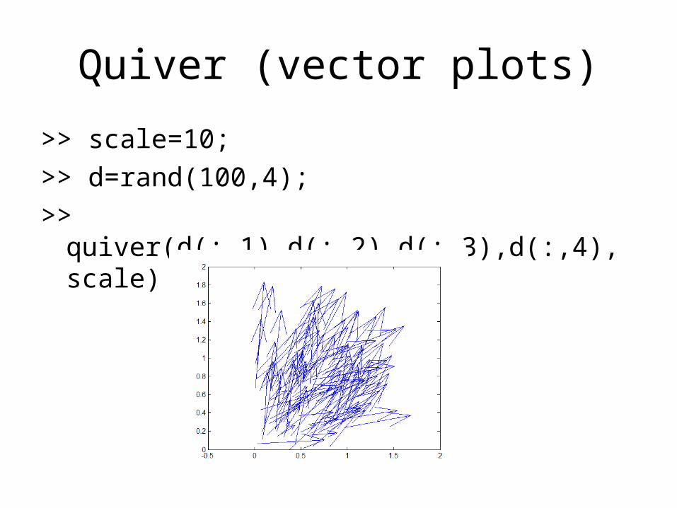
Quiver (vector plots)
>> scale=10;>> d=rand(100,4);>> quiver(d(:,1),d(:,2),d(:,3),d(:,4),scale)
Contours
• h=[…];• Contour(h)• Or Contour(x,y,h)
Contours w/labels
• C=[…];• [c,d]=contour(C);• clabel(c,d), colorbar
Numerical Partial Derivatives
• slope between points • MATLAB
– h=[]; (order assumed to be low y on top to high y on bottom!)
– [dhdx,dhdy]=gradient(h,spacing)
– contour(x,y,h)– hold– quiver(x,y,-dhdx,-dhdy)
Gradient Function and Streamlines• [dhdx,dhdy]=gradient(h);• [Stream]= stream2(X,Y,U,V,STARTX,STARTY);• [Stream]= stream2(-dhdx,-dhdy,
[51:100],50*ones(50,1));• streamline(Stream)• (This is for streamlines starting at y = 50 from x
= 51 to 100 along the x axis. Different geometries will require different starting points.)
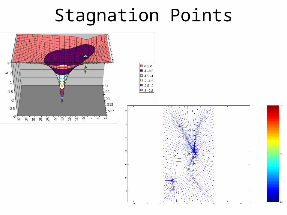
Stagnation Points
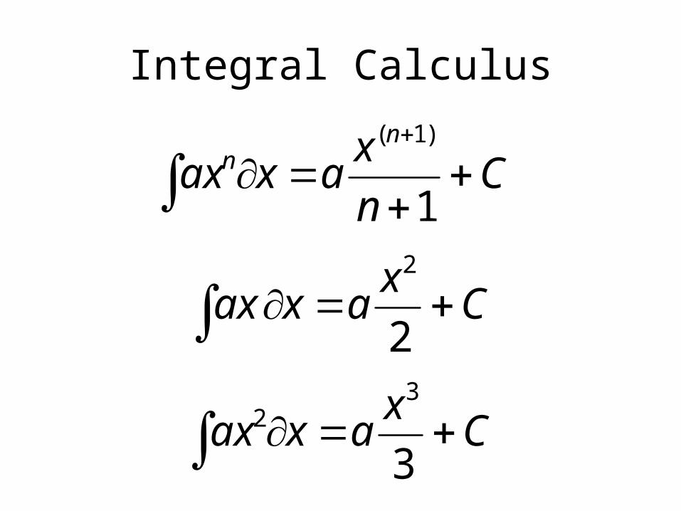
Integral Calculus
Cnxaxaxn
n
1
)1(
Cxaxax 2
2
Cxaxax 3
32
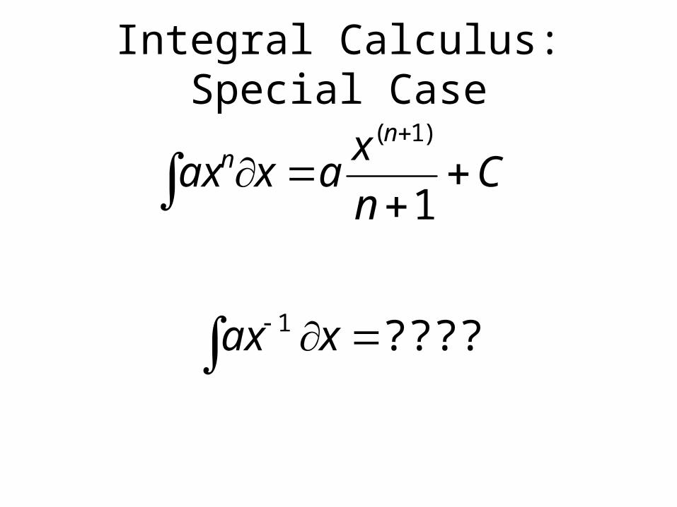
Integral Calculus: Special Case
Cnxaxaxn
n
1
)1(
????? 1 xax
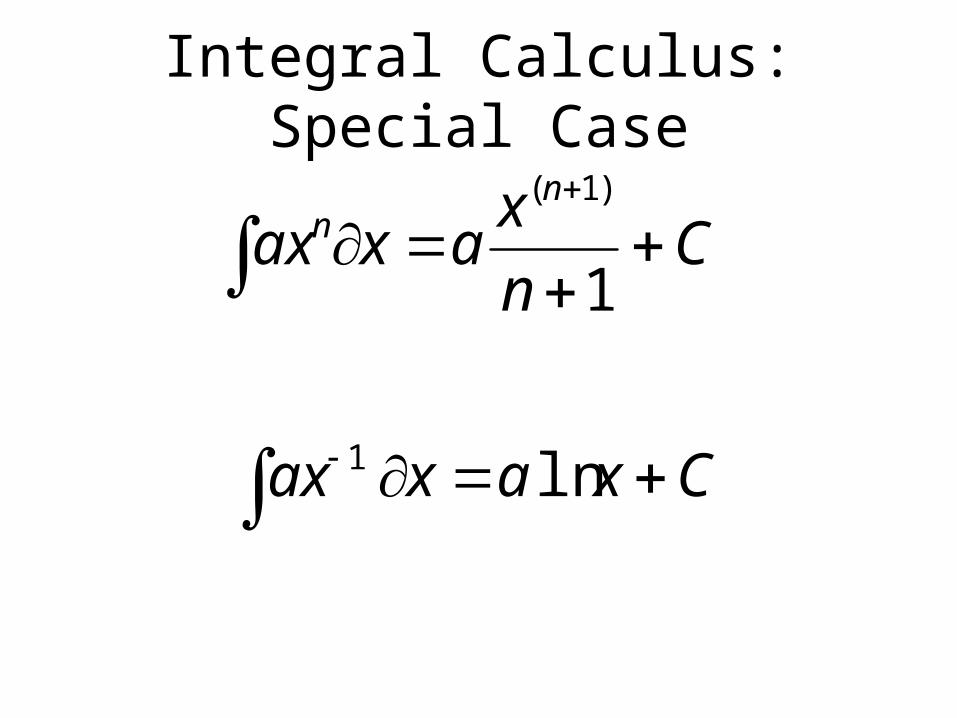
Integral Calculus: Special Case
Cnxaxaxn
n
1
)1(
Cxaxax ln 1