CALCULUS III: PROJECT 1A

1. Approximating Minima of a Function

1.1. Gradient Descent. For this project we will explore the method of finding a localminimum1 of a differentiable function called gradient descent. We have learned in classthat if a differentiable function f : Rn → R attains a relative minimum at a point p =(x1, x2, . . . , xn), then the gradient ∇f necessarily vanishes at p. But, solving the equation∇f(p) = 0 analytically might not be possible. For example, consider the function

f(x, y) = x6 + y6 + xy + (xy)4 + 1

The gradient of f is

∇f(x, y) = 〈6x5 + y + 4x3y4, 6y5 + x + 4x4y3〉so you would have to solve the system of equations

6x5 + y + 4x3y4 = 0

6y5 + x + 4x4y3 = 0

attempting which is not advised.

Figure 1.1. The graph of f .

The function f does attain a minimum though, as can be seen in figure 1.1, so wewould like to have a method for finding it.

Suppose you were hiking in the mountains and decided that you want to descend inthe most direct way. How would you go about doing it? A natural thing to do is to keepwalking in the direction of steepest descent. Recall that the gradient ∇f of a functionf points in the direction the function increases at the highest rate and −∇f pointsin the direction the function decreases at the highest rate. Therefore, if the functionf(x, y) denotes the height at the point with horizontal coordinates (x, y), the direction ofsteepest descent at the point with horizontal coordinates (x, y) is −∇f(x, y). To descendthe mountain we can follow the path whose horizontal projection is always tangent to−∇f as in figure 1.2b

1Finding a local maximum is completely analogous, but since the method is called gradient descent,we will stick to finding local minima.

1

CALCULUS III: PROJECT 1A 2

(a) The gradient of f at one point and thevector field −∇f .

(b) The flow line for−∇f and the correspond-ing path down the mountain.

We can apply the same reasoning to find the local minima of our first example. Westart at a random point (x, y) and we find the flow line for the vector field −∇f as infigure 1.3.2 Recall that a flow line for a vector field FFF is a path c(t) such that for all t,c′(t) = FFF (c(t)). In other words, the velocity vector of the path at each point c(t) equalsthe value of the vector field at that point.

Figure 1.3. The flow lines flow to the local minima. In this case, thereare two local minima and depending on your starting point you either endup at one or the other. (All vectors are drawn with the same length forease of viewing)

Viewing the flow lines in the x − y plane, we can estimate the location of the localminima to be approximately at (0.59,−0.59) and (−0.59, 0.59).

2It might happen that a flow line ends up at a saddle point instead of a local minimum. For example,consider the function f(x, y) = x2 − y2 and the flow line starting at (1, 0). This will not happen for a

generic starting point, so we will not consider it in this project.

CALCULUS III: PROJECT 1A 3

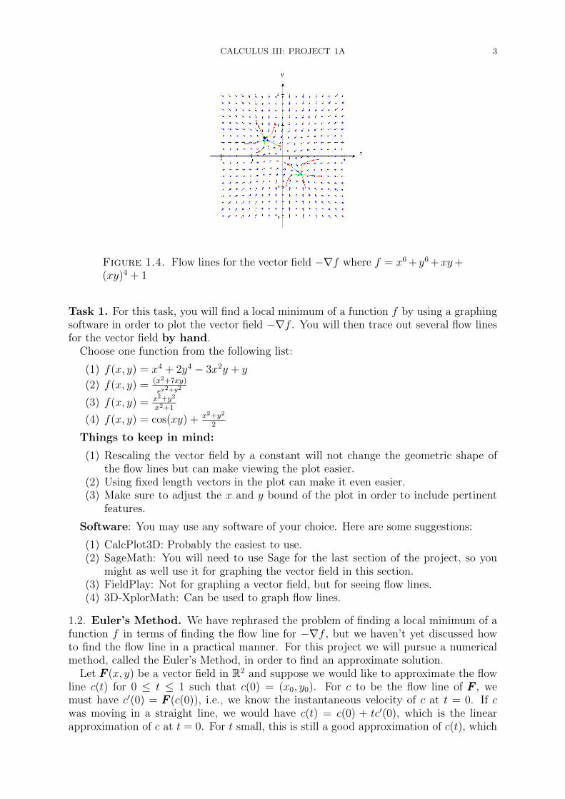
Figure 1.4. Flow lines for the vector field −∇f where f = x6 +y6 +xy+(xy)4 + 1

Task 1. For this task, you will find a local minimum of a function f by using a graphingsoftware in order to plot the vector field −∇f . You will then trace out several flow linesfor the vector field by hand.

Choose one function from the following list:

(1) f(x, y) = x4 + 2y4 − 3x2y + y

(2) f(x, y) = (x2+7xy)

ex2+y2

(3) f(x, y) = x2+y2

x2+1

(4) f(x, y) = cos(xy) + x2+y2

2

Things to keep in mind:

(1) Rescaling the vector field by a constant will not change the geometric shape ofthe flow lines but can make viewing the plot easier.

(2) Using fixed length vectors in the plot can make it even easier.(3) Make sure to adjust the x and y bound of the plot in order to include pertinent

features.

Software: You may use any software of your choice. Here are some suggestions:

(1) CalcPlot3D: Probably the easiest to use.(2) SageMath: You will need to use Sage for the last section of the project, so you

might as well use it for graphing the vector field in this section.(3) FieldPlay: Not for graphing a vector field, but for seeing flow lines.(4) 3D-XplorMath: Can be used to graph flow lines.

1.2. Euler’s Method. We have rephrased the problem of finding a local minimum of afunction f in terms of finding the flow line for −∇f , but we haven’t yet discussed howto find the flow line in a practical manner. For this project we will pursue a numericalmethod, called the Euler’s Method, in order to find an approximate solution.

Let FFF (x, y) be a vector field in R2 and suppose we would like to approximate the flowline c(t) for 0 ≤ t ≤ 1 such that c(0) = (x0, y0). For c to be the flow line of FFF , wemust have c′(0) = FFF (c(0)), i.e., we know the instantaneous velocity of c at t = 0. If cwas moving in a straight line, we would have c(t) = c(0) + tc′(0), which is the linearapproximation of c at t = 0. For t small, this is still a good approximation of c(t), which

CALCULUS III: PROJECT 1A 4

is the approximation we will use.

c(t) ≈ c(0) + tc′(0) = c(0) + tFFF (c(0))

Figure 1.5. Linear approximation to a path c(t).

Fixing a step size ∆t, we can approximate the value of c(∆t) by c(0) + ∆tFFF (c(0)) andthen repeat the process starting with c(∆t) instead of c(0). The algorithm then becomesthe following:

(1) Fix a step size ∆t.(2) Set c0 = c(0) = (x0, y0).(3) Compute

c1 = c0 + ∆tFFF (c0),

c2 = c1 + ∆tFFF (c1),

... =...

cn = cn−1 + ∆tFFF (cn−1)

(4) The result is the polygonal line with vertices c0, . . . , cn.

Figure 1.6. Example with FFF = 〈y,−x〉, (x0, y0) = (0, 1), and ∆t = 14

Note that the linear approximation gets better as ∆t gets smaller. But, making thestep size too small has the drawback that you need to perform more steps.

Task 2. Pick the following objects of your choice:

(1) A two-dimensional vector field FFF .(2) A starting point (x0, y0).

CALCULUS III: PROJECT 1A 5

(3) Step size ∆t.

Then, use the Euler method to find the approximate flow line c(t) of FFF with c(0) =(x0, y0). Compute at least 5 steps of the Euler process. Then, plot the vector field andthe corresponding polygonal line (either by hand or using a software). One conditionthat your vector field has to satisfy is that the points ci have to not lie on a line.

1.3. Imprecisions. Figure 1.6 shows that the solution obtained by Euler’s method, beingonly an approximation, can diverge from the actual flow line over time. This might seemto be a problem if we are trying to find a local minimum of a function f by approximatingthe flow of −∇f . It turns out to not be a problem: the Euler’s method approximationwill converge to the same minimal value of f even if along the way it diverges from theactual flow line. 3

One way to understand why that is the case is the following. Applying the Euler’smethod to −∇f , we get a sequence of points c0, c1, c2, . . . , cn. Each subsequent point isobtained by the formula ci+1 = ci + ∆t(−∇f(ci)), i.e., ci+1 is a small distance away fromci in the directions in which f is decreasing. Therefore, as long as ∆t is small enough,we have f(ci+1) < f(ci). In other words, we get a sequence of points with decreasingvalues of f . Eventually, we will approach the local minimum of f . Another thing to noteis that as ci approaches a local minimum, −∇f(ci) approaches 0, and therefore ci+1 − ciapproaches 0. In other words, once we are close enough to the local minimum, each stepof the Euler’s method only moves the point ci by a very small amount.

Figure 1.7. The flow line and the Euler’s method approximation with∆t = 1

4for f(x, y) = x2 + y2 + xy starting at (−1, 0)

3There are several caveats to this statement. The step size needs to be small enough and it mighthappen that the approximate flow line will converge to a different local minima than the original flowlines.

CALCULUS III: PROJECT 1A 6

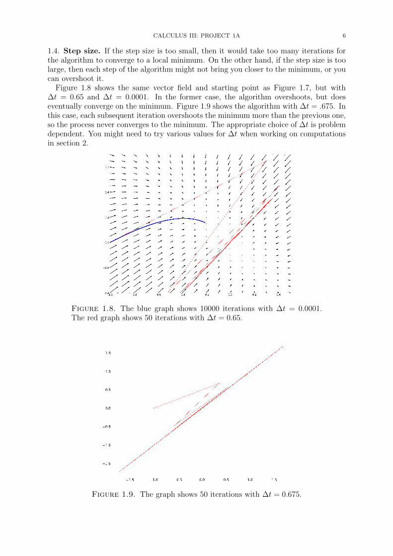
1.4. Step size. If the step size is too small, then it would take too many iterations forthe algorithm to converge to a local minimum. On the other hand, if the step size is toolarge, then each step of the algorithm might not bring you closer to the minimum, or youcan overshoot it.

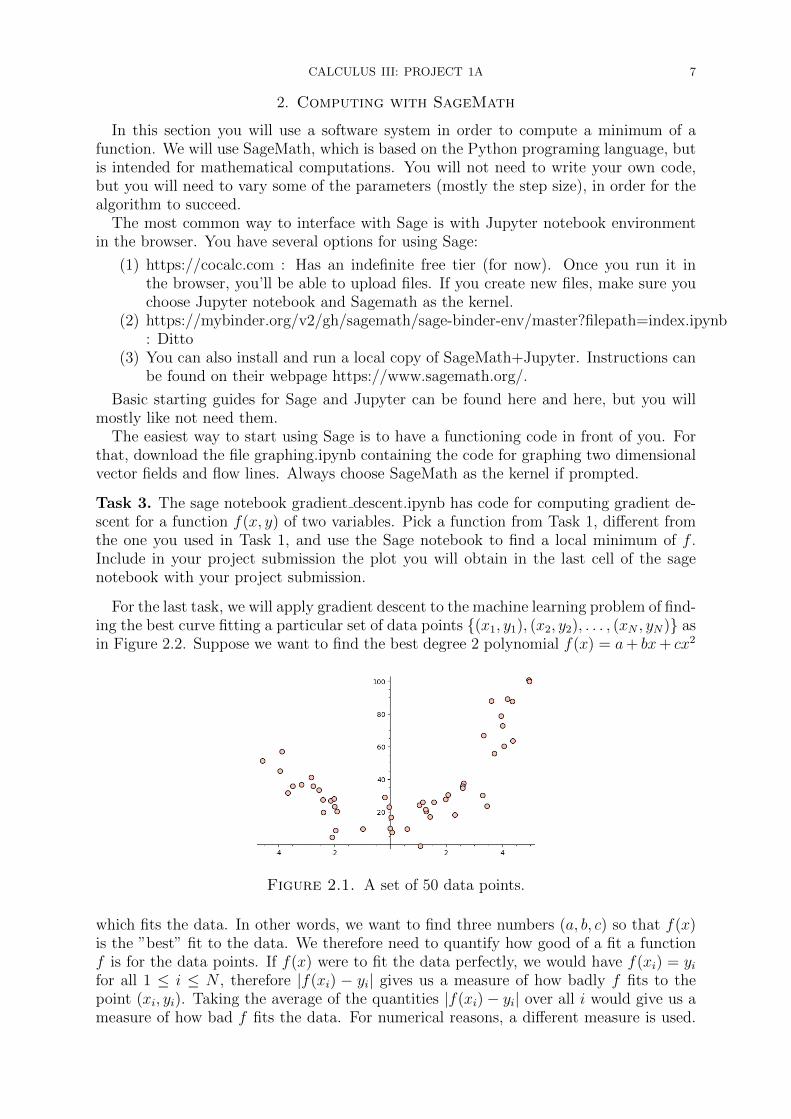
Figure 1.8 shows the same vector field and starting point as Figure 1.7, but with∆t = 0.65 and ∆t = 0.0001. In the former case, the algorithm overshoots, but doeseventually converge on the minimum. Figure 1.9 shows the algorithm with ∆t = .675. Inthis case, each subsequent iteration overshoots the minimum more than the previous one,so the process never converges to the minimum. The appropriate choice of ∆t is problemdependent. You might need to try various values for ∆t when working on computationsin section 2.

Figure 1.8. The blue graph shows 10000 iterations with ∆t = 0.0001.The red graph shows 50 iterations with ∆t = 0.65.

Figure 1.9. The graph shows 50 iterations with ∆t = 0.675.

CALCULUS III: PROJECT 1A 7

2. Computing with SageMath

In this section you will use a software system in order to compute a minimum of afunction. We will use SageMath, which is based on the Python programing language, butis intended for mathematical computations. You will not need to write your own code,but you will need to vary some of the parameters (mostly the step size), in order for thealgorithm to succeed.

The most common way to interface with Sage is with Jupyter notebook environmentin the browser. You have several options for using Sage:

(1) https://cocalc.com : Has an indefinite free tier (for now). Once you run it inthe browser, you’ll be able to upload files. If you create new files, make sure youchoose Jupyter notebook and Sagemath as the kernel.

(2) https://mybinder.org/v2/gh/sagemath/sage-binder-env/master?filepath=index.ipynb: Ditto

(3) You can also install and run a local copy of SageMath+Jupyter. Instructions canbe found on their webpage https://www.sagemath.org/.

Basic starting guides for Sage and Jupyter can be found here and here, but you willmostly like not need them.

The easiest way to start using Sage is to have a functioning code in front of you. Forthat, download the file graphing.ipynb containing the code for graphing two dimensionalvector fields and flow lines. Always choose SageMath as the kernel if prompted.

Task 3. The sage notebook gradient descent.ipynb has code for computing gradient de-scent for a function f(x, y) of two variables. Pick a function from Task 1, different fromthe one you used in Task 1, and use the Sage notebook to find a local minimum of f .Include in your project submission the plot you will obtain in the last cell of the sagenotebook with your project submission.

For the last task, we will apply gradient descent to the machine learning problem of find-ing the best curve fitting a particular set of data points {(x1, y1), (x2, y2), . . . , (xN , yN)} asin Figure 2.2. Suppose we want to find the best degree 2 polynomial f(x) = a+ bx+ cx2

Figure 2.1. A set of 50 data points.

which fits the data. In other words, we want to find three numbers (a, b, c) so that f(x)is the ”best” fit to the data. We therefore need to quantify how good of a fit a functionf is for the data points. If f(x) were to fit the data perfectly, we would have f(xi) = yifor all 1 ≤ i ≤ N , therefore |f(xi) − yi| gives us a measure of how badly f fits to thepoint (xi, yi). Taking the average of the quantities |f(xi)− yi| over all i would give us ameasure of how bad f fits the data. For numerical reasons, a different measure is used.

CALCULUS III: PROJECT 1A 8

Instead of taking the average of |f(xi) − yi|, we take the average of their squares. Thecorresponding function is called the mean square error. In other words, we have

MSE(a, b, c) =1

N

N∑i=1

(a + bxi + cx2i − yi)

2

This is the function we would like to minimize, and we can use the gradient descent forthat purpose. We have

∇MSE(a, b, c) =2

N

N∑i=1

(a + bxi + cx2i − yi)〈1, xi, x

2i 〉.

Figure 2.2. The best fitting degree 2 after 1000 iterations of gradientdescent.

Task 4. The sage notebook best fit.ipynb has code for computing the best fitting degree2 polynomial using gradient descent. For this task, you need to use Sage to find thebest fitting curve for the set of data generated randomly at http://math.jhu.edu/

~vzakhar2/teaching/spring2021/data.php. There is a clearly labeled cell in the Sagenotebook where you will need to copy and paste the data. You will have to adjust thestep size and the number of iteration in order to get a reasonable answer. Include in yourproject submission the plot of the function with the data points. You will need to adjustthe x bounds for your graph.