calculation of the free energy of crystalline solids · imperial college london calculation of the...
TRANSCRIPT

Imperial College London
Calculation of the free
energy of crystalline
solids
Manolis Vasileiadis
A thesis submitted for the Doctor of Philosophy degree of Imperial College London and for
the Diploma of Imperial College
Centre for Process Systems Engineering
Department of Chemical Engineering
Imperial College London
London SW7 2AZ
United Kingdom
28th
of November 2013

Abstract | i
Abstract
The prediction of the packing of molecules into crystalline phases is a key step
in understanding the properties of solids. Of particular interest is the phenomenon of
polymorphism, which refers to the ability of one compound to form crystals with
different structures, which have identical chemical properties, but whose physical
properties may vary tremendously. Consequently the control of the polymorphic
behavior of a compound is of scientific interest and also of immense industrial
importance. Over the last decades there has been growing interest in the development
of crystal structure prediction algorithms as a complement and guide to experimental
screenings for polymorphs.
The majority of existing crystal structure prediction methodologies is based on
the minimization of the static lattice energy. Building on recent advances, such
approaches have proved increasingly successful in identifying experimentally
observed crystals of organic compounds. However, they do not always predict
satisfactorily the relative stability among the many predicted structures they generate.
This can partly be attributed to the fact that temperature effects are not accounted for
in static calculations. Furthermore, existing approaches are not applicable to
enantiotropic crystals, in which relative stability is a function of temperature.
In this thesis, a method for the calculation of the free energy of crystals is
developed with the aim to address these issues. To ensure reliable predictions, it is
essential to adopt highly accurate molecular models and to carry out an exhaustive
search for putative structures. In view of these requirements, the harmonic
approximation in lattice dynamics offers a good balance between accuracy and
efficiency. In the models adopted, the intra-molecular interactions are calculated using
quantum mechanical techniques; the electrostatic inter-molecular interactions are
modeled using an ab-initio derived multipole expansion; a semi-empirical potential is
used for the repulsion/dispersion interactions. Rapidly convergent expressions for the
calculation of the conditionally and poorly convergent series that arise in the
electrostatic model are derived based on the Ewald summation method.
Using the proposed approach, the phonon frequencies of argon are predicted
successfully using a simple model. With a more detailed model, the effects of
temperature on the predicted lattice energy landscapes of imidazole and
tetracyanoethylene are investigated. The experimental structure of imidazole is

Abstract | ii
correctly predicted to be the most stable structure up to the melting point. The phase
transition that has been reported between the two known polymorphs of
tetracyanoethylene is also observed computationally. Furthermore, the predicted
phonon frequencies of the monoclinic form of tetracyanoethylene are in good
agreement with experimental data. The potential to extend the approach to predict the
effect of temperature on crystal structure by minimizing the free energy is also
investigated in the case of argon, with very encouraging results.
Declarations | iii
Declaration
I confirm that the work presented in this thesis is my own. Any information derived
from other sources is appropriately referenced.
Manolis Vasileiadis
The copyright of this thesis rests with the author and is made available under a
Creative Commons Attribution-Non Commercial-No Derivatives licence. Researchers
are free to copy distribute or transmit the thesis on the condition that they attribute it,
that they do not use it for commercial purposes and that they do not alter, transform of
build upon it. For any reuse or distribution, researchers must make clear to others the
licence terms of this work.

Acknowledgment | iv
Acknowledgments
The past four years have been a unique experience in my life. Without doubt
completing this Ph.D. would have not been possible without the support of many
people. I am grateful and I would like to thank my supervisors Prof. Claire Adjiman
and Prof. Costas Pantelides for their effort and support all these years, the ―crystal
prediction‖ team and especially Panos and Andrei, the Molecular Systems
Engineering group, my friends Vasilis, Esther, Apostolis, Thomas and Evangelia, my
―koumparous‖ and close friends Xenia and George, their son Leuteris, my parents
Michalis and Fotini and my brother Vasilis. Finally I am more than grateful to Eirini,
whose multiple contributions to this work and presence in my life are invaluable.
Manolis

Στοςρ γονείρ μος, Φωτεινή και Μισάλη

Contents | vi
Contents Abstract ........................................................................................................................... i
Declaration ................................................................................................................... iii
Acknowledgments......................................................................................................... iv
Contents ........................................................................................................................ vi
List of tables .................................................................................................................. ix
List of figures ................................................................................................................ xi
1. Introduction ............................................................................................................ 1
1.1. Polymorphism ................................................................................................. 1
1.2. Scope and outline ............................................................................................ 4
2. Crystals and free energy ......................................................................................... 6
2.1. Structure and classifications of crystals .......................................................... 6
2.2. Free energy—Definition ................................................................................. 7
2.3. Challenges in the calculation of the free energy ............................................. 9
2.4. Methods for the calculation of the free energy ............................................. 11
2.4.1. Overlap methods .................................................................................... 11
2.4.2. Thermodynamic integration ................................................................... 15
2.4.3. Expanded ensemble methods ................................................................. 23
2.4.4. Other methods ........................................................................................ 23
3. Lattice dynamics ................................................................................................... 25
3.1. Harmonic approximation............................................................................... 25
3.2. Assumptions and necessary conditions ......................................................... 30
3.3. The permissible wave vectors ....................................................................... 32
3.4. Normal modes & dispersion curves .............................................................. 34
3.5. Calculation of the free energy ....................................................................... 35
3.6. The density of vibrational states.................................................................... 40
3.7. Evaluation of the free energy expression ...................................................... 41
Contents | vii
3.8. The quasi-harmonic approximation .............................................................. 45
3.9. Applications of lattice dynamics ................................................................... 47
3.9.1. Inorganic crystals ................................................................................... 47
3.9.2. Organic molecular crystals .................................................................... 49
4. Molecular models ................................................................................................. 55
4.1. Intra-molecular interactions .......................................................................... 57
4.2. Pairwise additive potentials ........................................................................... 58
4.2.1. Energy .................................................................................................... 58
4.2.2. Dynamical matrix................................................................................... 62
4.3. Repulsion/dispersion interactions ................................................................. 64
4.4. Electrostatic interactions ............................................................................... 66
4.4.1. Electrostatic interactions using distributed multipoles .......................... 68
4.4.2. Orientation dependence of distributed multipoles ................................. 71
4.4.3. Derivatives of the electrostatic contributions ........................................ 73
4.5. Summary ....................................................................................................... 74
5. Evaluation of lattice sums..................................................................................... 75
5.1. The need for a ―lattice sum method‖ ............................................................. 75
5.2. Lattice sum methods...................................................................................... 77
5.3. Generalized Ewald summation method......................................................... 84
5.3.1. Calculation of the lattice energy of molecular crystals .......................... 90
5.3.2. Efficient summation scheme for the dynamical matrix ......................... 98
5.4. The Γ-point in the reciprocal space sum ..................................................... 107
6. Results ................................................................................................................ 110
6.1. The Lennard-Jones solid; Dispersion curves and density of states ............. 110
6.2. Crystal structure prediction methodology ................................................... 114
6.2.1. Overview of the approach .................................................................... 114
6.2.2. Comparison of crystal structures ......................................................... 115
Contents | viii
6.3. Imidazole ..................................................................................................... 116
6.3.1. Experimental information .................................................................... 116
6.3.2. Crystal structure prediction .................................................................. 117
6.3.3. Temperature effects in crystal structure prediction ............................. 120
6.4. Tetracyanoethylene ..................................................................................... 125
6.4.1. Experimental information .................................................................... 125
6.4.2. Crystal structure prediction .................................................................. 127
6.4.3. Calculation of the dispersion curves .................................................... 129
6.4.4. Temperature effects in crystal structure prediction ............................. 133
6.4.5. The effect of the molecular model on the lattice energy calculation ... 141
6.5. Quasi-harmonic free energy minimisation; Argon example revisited ........ 150
7. Conclusion and Perspectives .............................................................................. 153
7.1. Summary ..................................................................................................... 153
7.2. Future work ................................................................................................. 157
Conference presentations & publication .................................................................... 160
8. Bibliography ....................................................................................................... 162
Appendix A—Relations for the
tensor ..................................................... 195
Appendix B—The term
....................................................... 199

List of tables | ix
List of tables
Table 2-1 Summary of the most widely used thermodynamic potentials ...................... 9
Table 3-1 The coefficients and corresponding abscissas for Gauss-Legendre
quadrature. The density of sampling is limited to four nodes per direction. ............... 45
Table 4-1 Summary of all the contributions that are included in the electrostatic
interactions, when the multipole expansion is truncated at interactions of fourth order.
...................................................................................................................................... 71
Table 5-1 The self correction term for the different components of the various
contributions to the electrostatic energy gradient (equation 5-31). ............................. 99
Table 6-1 Basic characteristics of the unit cell of the two resolved forms of imidazole.
Lattice angles α and γ are equal to 90o for all forms at all temperature because of
symmetry constraints. ................................................................................................ 117
Table 6-2 Summary of the lattice energy, rank and the Helmholtz free energy of the α
and β forms of imidazole, as function of temperature. .............................................. 121
Table 6-3 Basic characteristics of the unit cell of the two resolved forms of TCNE.
Lattice angles α and γ are equal to 90o for all forms at all temperatures because of
symmetry constraints. ................................................................................................ 126
Table 6-4 The Helmholtz free energy A and rank of the cubic and monoclinic forms of
TCNE, as function of temperature T. The value of the global minimum free energy is
presented in the last column for comparison. In the bottom, the lattice energy and
rank of the relevant structures are also presented. Quantum mechanical calculations
were performed at the HF/6-31G(d,p) level. ............................................................. 135

List of tables | x
Table 6-5 Comparison of the unit cells of the two predicted forms of TCNE at M06
and HF level of theory. Lattice angle α is equal to 90o for all forms because of
symmetry constraints. ................................................................................................ 143
Table 6-6 The Helmholtz free energy A and rank of the cubic and monoclinic forms of
TCNE, as function of temperature T. The value of the global minimum free energy is
presented in the last column for comparison. In the bottom, the lattice energy and
rank of the relevant structures are also presented. Quantum mechanical calculations
were performed at the M06/6-31G(d,p) level. ........................................................... 144
Table 8-1 The self correction term for the different components of the contributions
up to second order to the electrostatic energy hessian (equation 5-34). .................... 201
Table 8-2 The self correction term for the different components of the contributions
from the third order to the electrostatic energy hessian (equation 5-34). .................. 202

List of figures | xi
List of figures
Figure 1-1 Two views of the crystal of α-glycine (Marsh, 1958), with the unit cell
indicated by a box. ......................................................................................................... 1
Figure 1-2 The chemical diagram and unit cell of (a) paracetamol and (b) ibuprofen,
two widely known pharmaceuticals. .............................................................................. 3
Figure 5-1 (a) The chemical diagram of tetracyanoethylene and (b) the experimental
unit cell of the monoclinic form at 298K. .................................................................... 93
Figure 5-2 The value of the charge-charge contribution to the electrostatic energy of
the calculated monoclinic form of tetracyanoethylene, as a function of the Ewald
convergence parameter. The direct space sum, the reciprocal space sum, the molecular
correction, and the self correction are also presented. Distributed multipoles were
derived at the M06/6-31G(d,p) level. .......................................................................... 94
Figure 5-3 The value of the charge-dipole contribution to the electrostatic energy of
the calculated monoclinic form of tetracyanoethylene, as function of the Ewald
convergence parameter. The direct space sum, the reciprocal space sum, and the
molecular correction are also presented. Distributed multipoles were derived at the
M06/6-31G(d,p) level. ................................................................................................. 95
Figure 5-4 The value of the charge-quadrupole contribution to the electrostatic energy
of the calculated monoclinic form of tetracyanoethylene, as function of the Ewald
convergence parameter. The direct space sum, the reciprocal space sum, and the
molecular correction are also presented. Distributed multipoles were derived at the
M06/6-31G(d,p) level. ................................................................................................. 96
Figure 5-5 The value of the dipole-dipole contribution to the electrostatic energy of
the calculated monoclinic form of tetracyanoethylene, as function of the Ewald
convergence parameter. The direct space sum, the reciprocal space sum, and the
molecular correction are also presented. Distributed multipoles were derived at the
M06/6-31G(d,p) level. ................................................................................................. 97

List of figures | xii
Figure 5-6 (a) The element of the dynamical matrix is related the interaction of
the red atom ( ) with the atom and its periodic images (green). (b) The
element of the dynamical matrix is related to the self-interaction of the green
atoms ( ) ..................................................................................................... 101
Figure 5-7 The value of the component (0,1s) of the charge-dipole contribution to the
element of matrix (defined in equation 4-22, page 63), for
as function of the Ewald convergence parameter α. The calculation is
performed for the predicted structure that corresponds to the monoclinic form of
tetracyanoethyelene (see section 6.4.2). The quantum mechanical calculations were
performed at the M06/6-31G(d,p) level. The direct space sum and the reciprocal space
sum are also shown. ................................................................................................... 103
Figure 5-8 A projection onto the complex plane of the dynamical matrix element
shown in Figure 5-7. The correction term and the direct and reciprocal space sums are
also shown. ................................................................................................................. 104
Figure 5-9 The value of the component (0,2c) of the charge-quadruple contribution to
the element of matrix (defined in equation (4-22), page 63), for
as a function of the Ewald convergence parameter α. The calculation
is performed for the predicted structure that corresponds to the monoclinic form of
tetracyanoethyelene (see section 6.4.2). The quantum mechanical calculations were
performed at the M06/6-31G(d,p) level. The direct space sum and the reciprocal space
sum are also shown. ................................................................................................... 105
Figure 5-10 A projection onto the plane defined by the real part of the dynamical
matrix element shown in Figure 5-9, and the α parameter. The correction term and the
direct and reciprocal space sums are also shown. ...................................................... 106
Figure 6-1 Dispersion curves of Argon when the wave vectors vary along three
directions , , and , as a function of the reduced wave vector
coordinate . The dots are the calculated points, while the triangles are experimental
data (Fujii et al., 1974).. ............................................................................................. 112

List of figures | xiii
Figure 6-2 (a) Normalized density of vibrational sates as a function of frequency; (b) a
close-up of the normalized density of states in the low frequency region. A quadratic
trend curve is is also fitted to the low frequency region and shown in red. ............... 113
Figure 6-3 The molecular diagram of imidazole. ...................................................... 116
Figure 6-4 Visualisation of the experimental unit cells of the two forms of imidazole
a) the unit cell of the α-form at 103 K and ambient pressure (McMullan et al., 1979) ;
b) the unit cell of the β-form at 298K and 0.8GPa (Paliwoda et al., 2012). ............. 117
Figure 6-5 Final lattice energy landscape of imidazole. Red dot and diamond
represent the experimentally known α and β forms. Quantum mechanical calculations
were performed at M06/6-31G(d,p) level. ................................................................. 119
Figure 6-6 Overlay between the predicted (green) and experimental (coloured by
element) forms of imidazole. a) the α-form, with rms15=0.133Å, b) the β-form, with
rms15=0.425Å. Quantum mechanical calculations were performed at the Μ06/6-
31G(d,p) level.. .......................................................................................................... 119
Figure 6-7 The Helmholtz free energy landscape of imidazole at (a) 0 K ; (b) 100 K.
All necessary quantum mechanical (charge density and geometry) calculations were
performed at M06/6-31G(d,p) level. The colour scale describes the difference in the
rank of each structure before and after the vibrational contributions are included. .. 122
Figure 6-8 The Helmholtz free energy landscape of imidazole at (a) 200K ; (b) 300K.
All necessary quantum mechanical (charge density and geometry) calculations were
performed at M06/6-31G(d,p) level. The colour scale describes the difference in the
rank of each structure before and after the vibrational contributions are included. .. 123
Figure 6-9 The Helmholtz free energy landscape of imidazole at 350K. All necessary
quantum mechanical (charge density and geometry) calculations were performed at
M06/6-31G(d,p) level. The colour scale describes the difference in the rank of each
structure before and after the vibration contributions are included. .......................... 124

List of figures | xiv
Figure 6-10 a) The molecular diagram of tetracyanoethylene ; b) A visualisation of
the geometry of the isolated molecule of TCNE obtained by quantum mechanical
calculations at MP2/6-31G(d,p) level. ....................................................................... 125
Figure 6-11 Visualization of the experimental unit cells of the two forms of
tetracyanoethylene. a) the unit cell of the cubic form at 298K (Little et al., 1971); b)
the unit cell of the monoclinic form also at 298K (Chaplot et al., 1984). ................. 126
Figure 6-12 Final lattice energy landscape of TCNE. The red dot and diamond
represent the monoclinic and cubic experimentally known forms. Quantum
mechanical calculation were performed at HF/6-31G(d,p) level. .............................. 128
Figure 6-13 Overlay of the two known experimental forms of TCNE (coloured by
element) and the corresponding predicted structures (green). a) the cubic form
compares to the experimental with an rms15=0.039Å; b) the predicted monoclinic
form is different from the experimental by an rms15=0.285Å. Quantum mechanical
calculations were performed at the HF/6-31G(d,p) level. ......................................... 129
Figure 6-14 Dispersion curves of TCNE. The three panels correspond to different
wave vectors as indicated at the top. The 12 lowest energy branches represent the
external modes of vibration while the remaining branches represent the internal
modes. ........................................................................................................................ 131
Figure 6-15 Comparison of the 8 experimentally determined lowest frequency modes
of vibration of TCNE (in red) with the corresponding calculated modes (in black).
The wave vector varies along directions , and . ................... 132
Figure 6-16 Comparison of the 4 experimentally determined highest frequency
external modes of vibration of TCNE (in red) with the corresponding calculated
modes (in black). The wave vector varies along directions , and
. ...................................................................................................................... 133

List of figures | xv
Figure 6-17 The Helmholtz free energy landscape of tetracyanoethylene at (a) 0 K ;
(b) 50 K. All necessary quantum mechanical (charge density and geometry)
calculations were performed at HF/6-31G(d,p) level. The colour scale describes the
difference in the rank of each structure before and after the vibrational contributions
are included. ............................................................................................................... 136
Figure 6-18 The Helmholtz free energy landscape of tetracyanoethylene at (a) 100 K ;
(b) 200 K. All necessary quantum mechanical (charge density and geometry)
calculations were performed at HF/6-31G(d,p) level. The colour scale describes the
difference in the rank of each structure before and after the vibrational contributions
are included. ............................................................................................................... 137
Figure 6-19 The Helmholtz free energy landscape of tetracyanoethylene at (a) 300 K ;
(b) 400 K. All necessary quantum mechanical (charge density and geometry)
calculations were performed at HF/6-31G(d,p) level. The colour scale describes the
difference in the rank of each structure before and after the vibrational contributions
are included. ............................................................................................................... 138
Figure 6-20 The Helmholtz free energy landscape of tetracyanoethylene at (a) 450 K
(b) 500 K. All necessary quantum mechanical (charge density and geometry)
calculations were performed at HF/6-31G(d,p) level. The colour scale describes the
difference in the rank of each structure before and after the vibrational contributions
are included. ............................................................................................................... 139
Figure 6-21 The free energy difference between the cubic and monoclinic forms of
TCNE as function of temperature. The red dashed line is a linear interpolation of the
free energy difference in the region of temperatures between 60K and the melting
point. The transition temperature is obtained as the solution of the equation on the
plot, setting y to 0....................................................................................................... 140
Figure 6-22 The free energy difference between the structure that corresponds to the
monoclinic form and structure #24 as a function of temperature. The red dashed line
is a linear interpolation of the free energy difference in the region of temperatures

List of figures | xvi
between 60K and the melting point. The transition temperature is obtained as solution
of the equation on the plot setting y to 0. ................................................................... 140
Figure 6-23 Overlay of the predicted and experimental forms of TCNE. a) the cubic
form matches the experimental with an rms15=0.103Å, b) the predicted monoclinic
form matches the experimental form with an rms15=0.299Å. Quantum mechanical
calculations were performed at the M06/6-31G(d,p) level of theory. ....................... 142
Figure 6-24 Final lattice energy landscape of TCNE. Red dot and diamond represent
the monoclinic and cubic experimentally known forms. Quantum mechanical
calculation were performed at M06/6-31G(d,p) level. .............................................. 142
Figure 6-25 Dispersion curves of TCNE. The 12 lowest energy branches represent the
external modes of vibration while the remaining branches represent the internal
modes. Quantum mechanical calculations were performed at the M06/6-31G(d,p)
level of theory. ........................................................................................................... 145
Figure 6-26 Comparison of the 8 experimentally determined lowest frequency modes
of vibration of TCNE (in red) with the corresponding calculated modes (in black).
The wave vector varies along directions , and . Calculations
were carried out at the M06/6-31G(d,p) level of theory ............................................ 146
Figure 6-27 Comparison of the 4 experimentally determined highest frequency
external modes of vibration of TCNE (in red) with the corresponding calculated
modes (in black). The wave vector varies along directions , and
. Calculations were carried out at the M06/6-31G(d,p) level of theory. ........ 147
Figure 6-28 The Helmholtz free energy landscape of tetracyanoethylene at (a) 0 K ;
(b) 100 K. All necessary quantum mechanical (charge density and geometry)
calculations were performed at M06/6-31G(d,p) level. The colour scale describes the
difference in the rank of each structure before and after the vibrational contributions
are included. ............................................................................................................... 148

List of figures | xvii
Figure 6-29 The Helmholtz free energy landscape of tetracyanoethylene at (a) 200 K ;
(b) 300 K. All necessary quantum mechanical (charge density and geometry)
calculations were performed at M06/6-31G(d,p) level. The colour scale describes the
difference in the rank of each structure before and after the vibration contributions are
included. ..................................................................................................................... 149
Figure 6-30 The lattice constant of argon as function of temperature.. ..................... 152
Figure 6-31 The thermal expansion coefficient of argon as function of temperature.
.................................................................................................................................... 152

Chapter 1. Introduction | 1
Figure 1-1 Two views of the crystal of α-glycine (Marsh, 1958), with the unit cell indicated
by a box.
1. Introduction
1.1. Polymorphism
Solid materials can be either amorphous or crystalline. Crystals are unique
because they exhibit long range spatial order in all directions, in contrast to
amorphous solids. An example is shown in Figure 1-1, where the crystal of α-glycine
(Marsh, 1958) can be seen. The ordered packing of crystals is a key characteristic that
essentially distinguishes the crystalline phases from other types of phases such as
liquid and gas. In addition, the ordered packing is the reason why most of the physical
properties of crystalline solids are anisotropic, i.e., depend on direction. The other
major states (liquids and gases), with the notable exception of liquid crystals which
exhibit a degree of order, have an isotropic structure and thus also have isotropic
properties.
A phenomenon related to the crystalline state is polymorphism. This term
describes the ability of any compound, inorganic or organic, to arrange itself in more
than one crystal structure; these different structures are referred to as the polymorphs
of the compound. The most common and one of the earliest examples of
Chapter 1. Introduction | 2
polymorphism, dating back to the early 19th
century, is the discovery of the existence
of two allotropic forms of carbon, diamond and graphite (McCrone, 1965). The
importance, industrial and academic, of polymorphism arises from the fact that
different polymorphs have different physical properties. For example the melting
point of diamond is close to 3900oC, while graphite disintegrates above 700
oC.
Furthermore, graphite is an electric conductor along a specific direction, while
diamond is not. As McCrone noted in a widely quoted statement (McCrone, 1965):
“It is at least this author’s opinion that every compound has different polymorphic
forms and that, in general the number of forms known for a given compound is
proportional to the time and money spent in research on that compound.”
I believe the following is an equally important and instructive phrase in McCrone‘s
(1965) text:
“…different polymorphs of a given compound are, in general, as different in structure
and properties as the crystals of two different compounds…”
Many solid state industrial products such as agrochemicals and pharmaceuticals
are produced in crystalline form. Pharmaceuticals such as paracetamol (Figure 1-2, a)
or ibuprofen (Figure 1-2, b) are common examples of organic molecular crystals of
industrial relevance. The understanding of the dependence of the properties of the
product on its structure is key for the design and manufacturing of crystalline
products. The implications of polymorphism in pharmaceutical development have
been described by many authors (Campeta et al., 2010; Chekal et al., 2009; Hilfiker
2006). The most notorious example of the impact of polymorphism in the production
of pharmaceuticals is that of ritonavir (Chemburkar et al, 2000; Bauer et al., 2001), a
novel anti-HIV drug developed by Abbott Laboratories, for which a more stable
polymorph appeared years after the start of production. The new form was much less
soluble, and much more stable. The significantly different solubility required a new
design for both product formulation and production. This incident threatened the
supply of the drug to patients. There are also other examples of the appearance of a
new polymorph during the late stage of drug development (Desikan et al. 2005), albeit
with less impact on drug development and production.

Chapter 1. Introduction | 3
(a)
(b)
Figure 1-2 The chemical diagram and unit cell of (a) paracetamol and (b) ibuprofen,
two widely known pharmaceuticals.
It is evident that the control and prediction of the polymorphic landscape, i.e. the
relative stability of different polymorphs, is not only academically interesting, but is
also crucial for industry. The exploration of the polymorphic landscape is usually
done through experimental screening for polymorphs. Unfortunately this task, in
addition to being costly, cannot guarantee that all polymorphs (stable and metastable)
have been found, nor that the thermodynamically most stable polymorph for a given
compound for given temperature and pressure conditions is known. Therefore there
has been a growing interest in the development of crystal structure prediction

Chapter 1. Introduction | 4
techniques as a tool complementary to the experimental screening for polymorphs. In
crystal structure prediction the aim is to identify all (stable and metastable)
polymorphs into which a compound may crystallise. The determination of the relative
thermodynamic stability of the polymorphs of the compound is also required as part
of the investigation of the polymorphic landscape.
1.2. Scope and outline
The vast majority of the methods that aim to tackle the problem of crystal
structure prediction are based on static lattice energy minimisation algorithms (Day,
2011; Price 2008). Based on these algorithms, it is in general possible to predict the
structure of small molecules with limited flexibility (Bardwell et al., 2010; Day et al.,
2005, 2009; Motherwell et al. 2002; Lommerse et al. 2000). Furthermore recent
advances, mainly in the handling of flexibility (Kazantsev et al., 2010, 2011:a), have
allowed the successful prediction of the crystal of a large flexible molecule that
resembles those of pharmaceutical interest (Bardwell et al., 2010; Kazantsev et al.,
2011:b). Despite their success the applicability of these algorithms is limited to
monotropically-related polymorphs. The relative stability of enantiotropically-related
polymorphs is a function of temperature (McCrone, 1965), and therefore they cannot
be studied by consideration of the lattice energy only, as this restricts the calculations
to 0 K.
In this thesis a method for the calculation of the free energy of crystal structures
is presented, and integrated into a lattice energy based crystal structure prediction
technique. The purpose of the work is to design a methodology that would allow the
prediction of the thermodynamically stable crystal structure as function of
temperature without dependence on experimentally available structures for the
compound of interest.
Some fundamentals of crystallography and a brief survey of the most widely used
free energy methods are presented in chapter 2. In chapter 3 the calculation of the free
energy using the method of lattice dynamics under harmonic approximation is
described in detail. Furthermore useful concepts of the dynamical theory of crystal
lattices are introduced.

Chapter 1. Introduction | 5
The molecular models adopted in the calculations involved in this thesis are presented
in chapter 4. The modeling approach is chosen as a compromise between the
conflicting requirements of high accuracy and reasonable computational cost.
When static or dynamical calculations are performed in crystals usually one
encounters the problem of the evaluation of lattice sums, i.e. infinite summations over
all the unit cells of the crystal. In chapter 5 a method based on the Ewald summation
technique is developed to perform the necessary lattice sums.
Lattice dynamics and free energy calculations are performed on computationally
generated crystals including argon and two small rigid organic molecules, imidazole
and tetracyanoethylene. The crystal structures are generated by the CrystalPredictor
algorithm and, for the organic molecules, ranked using the more sophisticated
electrostatic models in the DMACRYS package. Furthermore the free energy of the
fcc crystal of argon is minimised at various temperatures from 0 K to 84 K. The
results of these calculations are presented in chapter 6.
Finally some concluding remarks are presented in chapter 7. Directions for future
work are also suggested.
Chapter 2. Crystals and free energy | 6
2. Crystals and free energy
2.1. Structure and classifications of crystals
The structure of crystals is periodic, allowing their description by means of a unit
cell, usually defined by three lattice vectors (or equivalently by three lattice lengths
and three lattice angles), the number of molecules in the unit cell, and the positions of
all the atoms in the cell. By translation of the unit cell along the three lattice vectors, it
is possible to obtain the coordinates of all the remaining atoms in the crystal. The unit
cell for -glycine is shown as a box in Figure 1-1. The atomic positions within the
unit cell can be defined in many equivalent ways; this has been extensively discussed
elsewhere (Karamertzanis, 2004).
In crystallography crystals are categorized based on the symmetry properties they
exhibit. Here I briefly describe those terms that are useful for the purpose of this
thesis. More detailed information on the subject of symmetry can be found in several
textbooks e.g. (McWeeny, 1963). There are two kinds of symmetry properties. In the
first kind are operations that leave only one point of the crystal unmoved. Such
symmetry operations are the so-called proper and improper rotations, which form
groups that are commonly known as point groups. Reflection and inversion are
special cases of improper rotations. The other kind of symmetry operations that is
found in crystals does not leave any point of the crystal at its original position. Those
are translations along the three vectors that define the crystal lattice. Sets that are
composed of point group operations and translations are called space groups. Space
groups can describe fully the symmetry properties of crystalline solids, and therefore
crystals are classified based on their space group. One important concept is that of the

Chapter 2. Crystals and free energy | 7
symmetry element, which should not be confused with the symmetry operation. The
symmetry element is the ―reference‖ with respect to which a symmetry operation is
defined. For example if rotation is performed about the y-axis, the y-axis is the
symmetry element. Another example of a symmetry element is the point with respect
to which an inversion is performed.
The symmetry operations that form a point group within a space group must be
compatible with each other. For example the rotations that compose a point group
must be such that, when an operation is performed, the symmetry elements of the
object must be transformed into new symmetry elements. As a result, only 32 of the
possible point groups can be sub-groups of a space group as a consequence of the
presence of translational symmetry. Each of these point groups defines a crystal class.
Each of the crystal classes may belong to one of the 7 crystal systems and one of the
14 Bravais lattices. The term ―crystal system‖ is defined by the point group associated
with the empty lattice of a crystal if it is described by a primitive unit cell (i.e. only
one point is included in each unit cell). There are seven point groups that are
compatible with an empty lattice and they define the following crystal systems: cubic,
tetragonal, hexagonal, rhombohedral, orthorhombic, monoclinic, and triclinic. The 14
Bravais lattices include the 7 primitive lattices in each crystal system and 7 more
lattices described by non-primitive (off-centred) unit cells. The seven non primitive
lattices are the body centred cubic (bcc), the face centred cubic (fcc), the body centred
rhombohedral, the face centred orthorhombic, the base centred orthorhombic, the
body centred orthorhombic, and the base centred monoclinic. In general not all 32
point groups defining a crystal class are compatible with every one of the 14 Bravais
lattices. As a result it can be proven that only 230 space groups can be formed.
2.2. Free energy—Definition
The general framework of chemical thermodynamics can be used to describe any
system by means of the so-called characteristic function:
d
(2-1)

Chapter 2. Crystals and free energy | 8
Equation (2-1) gives the internal energy, , of a system of components as function
of the entropy , volume and the number of particles of each component , its
natural variables. , and are the temperature, pressure and chemical potential of
component respectively. They are related to the natural variables of by:
(2-2)
Although the characteristic function provides information that allows the full
description of the system by means of the formalism of the chemical thermodynamics,
in most cases this function is not known. For example, the lack of a direct method for
the measurement of entropy hinders its use.
As a result it is common practice to work using a thermodynamic potential or
fundamental equation instead of the internal energy (McQuarrie, 2000; Sandler,
1999). A thermodynamic potential is a function that contains all the information
included in the characteristic function but whose natural variables are different. The
most convenient choice of thermodynamic potential function depends on the
application. Thermodynamic potentials are constructed as Legendre transforms of the
internal energy (McQuarrie, 2000):
(2-3)
where and represent any of the natural variables of the internal energy and is
the thermodynamic potential obtained. The most widely used thermodynamic
potentials are summarized in Table 3-1.

Chapter 2. Crystals and free energy | 9
Thermodynamic
potential Symbol Legendre transform Natural Variables
Helmholtz free energy A
Enthalpy H
Gibbs free energy G =
Grand potential Ω Ω
Table 2-1 Summary of the most widely used thermodynamic potentials.
According to chemical thermodynamics, for a system at equilibrium each
thermodynamic potential is minimum when its natural variables have been
constrained (Sandler, 1999). If for example the volume, temperature and particle
numbers are specified for a closed system then the Helmholtz free energy is at a
minimum when the system reaches equilibrium. On the other hand if pressure,
temperature and particle numbers are specified the Gibbs free energy is at a minimum
when the system reaches equilibrium.
2.3. Challenges in the calculation of the free
energy
Statistical mechanics (Hill, 1986; McQuarrie, 2000) provides the formalism for
the macroscopic description of a system using information on its microscopic states.
The ensemble is the core concept of statistical thermodynamics. An ensemble is a
virtual collection of a large number of replicas of the system, each one compatible
with the macroscopic state of the system being studied. Some of the most common
ensembles are the canonical ensemble (or ensemble) defined by specification
of the number of particles, volume and temperature, the grand canonical ensemble (or
ensemble) where volume, temperature and chemical potential are constrained
and the isothermal isobaric ensemble (or ensemble), where the macroscopic
properties specified are the number of particles, the pressure and the temperature. The
number of times each microscopic state is found in an ensemble is proportional to its
probability, which is defined by statistical mechanics. Details of the probability
distribution in each ensemble can be found in the standard textbooks (Allen &

Chapter 2. Crystals and free energy | 10
Tildesley, 1987; Frenkel & Smit, 2002; Hill, 1986; McQuarrie, 2000). The
normalization factor of the probability distribution is known as the partition function,
.
In general the free energy, whose natural variables are the defining quantities of a
statistical ensemble, is associated with the partition function of the ensemble with an
equation of the form (Allen & Tildesley, 1987; Hill, 1986; McQuarrie, 2000):
(2-4)
In the canonical ensemble for example the Helmholtz free energy is given by:
(2-5)
while the Gibbs free energy is given by:
(2-6)
where is the Boltzmann constant.
Thus in principle the ―absolute‖ free energy could be calculated with a standard
molecular simulation. Unfortunately this is not the case. The canonical partition
function for example can be expressed as an ensemble average (Allen & Tildesley,
1987; Lyubartsev et al., 1992):
(2-7)
where the notation indicates a canonical ensemble average, obtained in a
Metropolis Monte Carlo or a molecular dynamics simulation (Allen & Tildesley,
1987; Frenkel & Smit, 2002). Since the configuration space is sampled proportionally
to the Boltzmann factor:
(2-8)

Chapter 2. Crystals and free energy | 11
the quantity
(which is the reciprocal to the Boltzmann factor) in the
configurations that are sampled more often is small. In contrast the configurations
whose
value is high are only rarely sampled, and therefore the estimate of the
average in equation (2-7) would be very poor.
2.4. Methods for the calculation of the free
energy
In order to overcome the difficulties in the calculation of the free energy many
ingenious algorithms have been designed. Their common characteristic is that they
aim to calculate a free energy difference instead of an ―absolute‖ free energy. The
various free energy methods are going to be categorized in a way similar to Kofke &
Cummings (1998). Three broad categories are identified, (a) the overlap methods (b)
the thermodynamic integration methods and (c) the expanded ensemble methods. In
this section some of the methods that can be found in the literature and can be
potentially used for the calculation of the free energy of a crystal are summarized.
2.4.1. Overlap methods
Zwanzig (1954) proposed the free energy perturbation method for the calculation
of free energy differences. The method was originally presented as a perturbation
theory for the calculation of the thermodynamic properties of a system. The free
energy difference between two systems ―0‖ (the reference) and ―1‖ (the system of
interest) is calculated as:
(2-9)
where and denotes an average over the ensemble of the
reference system. It is important to note that in equation (2-9) the subscripts may be
interchanged, having as a consequence the requirement of sampling the distribution of
system ―1‖.

Chapter 2. Crystals and free energy | 12
The calculation of the free energy by means of equation (2-9) is often very
difficult. Free energy perturbation offers an efficient calculation method for the free
energy if the important region of the configuration space of the reference system and
the system of interest overlap sufficiently (Allen & Tildesley, 1987; Frenkel & Smit,
2002). A method that was proposed in order to tackle this problem is umbrella
sampling (Torrie & Valeau, 1974, 1976; Valleau & Card, 1972). In umbrella
sampling, a calculation of the free energy is performed via an average
according to a distribution modified by a weighting function . The bias introduced is
then removed and the calculation of the free energy is performed as:
(2-10)
The modified distribution is necessary to have a ―bridging‖ property i.e. to
overlap (almost completely) with both the distributions of the systems ―0‖ and ―1‖. It
is adjusted so that it is nearly uniform. Umbrella sampling can also be applied in a
multistage fashion (Valleau & Card, 1972).
Bennett in 1976 proposed the acceptance ratio method in order to overcome the
difficulties associated with the calculation of the free energy differences. He wrote the
ratio of the configurational integral of the two systems ―0‖ and ―1‖ as:
(2-11)
and determined the weighting function that minimizes the variance of the free
energy calculation. The functional form of the optimal comprises a parameter, ,
that has the physical significance of a shift of the potential energy. The determination
of the optimal parameter is done in a self-consistent, iterative, way. Note that in
contrast to umbrella sampling, the acceptance ratio method requires the performance
of two simulations for the estimation of the free energy difference.
In the same paper (Bennett,1976) the interpolation or curve fitting method is also
presented. In this method during the two Monte Carlo runs necessary for the

Chapter 2. Crystals and free energy | 13
evaluation of (2-11) the histograms and are stored. These show the
probability of generating microstates with energy difference when sampling the
Boltzmann distributions of systems ―0‖ and ―1‖ respectively. Nearly identical
polynomials are then fitted to both histograms, with the only difference being the
constant terms. The free energy is then estimated as the difference of the constant
terms. The method of Bennett is also found in literature under the name overlapping
distribution method (Frenkel & Smit, 2002). Bennett uses the term ―overlap methods‖
to describe all the methods mentioned so far in this section as a general category
within free energy methods.
Kofke and co-workers (Kofke & Cummings, 1997, 1998; Lu & Kofke, 1999)
adopted a different point of view from the previously mentioned methods. They
pointed out the similarities between them and classified umbrella sampling and
acceptance ratio methods as staged versions of the free energy perturbation method,
where an intermediate system is used to facilitate the calculation. They also suggested
that it is more efficient to adopt a free energy method where sampling is performed
according to the distribution of the higher entropy system. The authors call this
approach sampling in the ―insertion‖ direction by analogy to Widom‘s test particle
insertion method (Widom, 1963). When the distribution of the lower entropy system
is sampled they refer to sampling in the ―deletion‖ direction. Based on this way of
thinking they also proposed two analogous schemes for the calculation of the free
energy, namely staged deletion (or annihilation) and staged insertion. In the former
scheme, the energy difference is obtained as:
(2-12)
where ―1‖ is assumed to be the system of lower entropy and in staged insertion, it is
given by:
(2-13)
Chapter 2. Crystals and free energy | 14
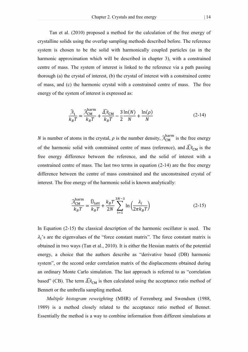
Tan et al. (2010) proposed a method for the calculation of the free energy of
crystalline solids using the overlap sampling methods described before. The reference
system is chosen to be the solid with harmonically coupled particles (as in the
harmonic approximation which will be described in chapter 3), with a constrained
centre of mass. The system of interest is linked to the reference via a path passing
thorough (a) the crystal of interest, (b) the crystal of interest with a constrained centre
of mass, and (c) the harmonic crystal with a constrained centre of mass. The free
energy of the system of interest is expressed as:
(2-14)
is number of atoms in the crystal, is the number density,
is the free energy
of the harmonic solid with constrained centre of mass (reference), and is the
free energy difference between the reference, and the solid of interest with a
constrained centre of mass. The last two terms in equation (2-14) are the free energy
difference between the centre of mass constrained and the unconstrained crystal of
interest. The free energy of the harmonic solid is known analytically:
(2-15)
In Equation (2-15) the classical description of the harmonic oscillator is used. The
‘s are the eigenvalues of the ―force constant matrix‖. The force constant matrix is
obtained in two ways (Tan et al., 2010). It is either the Hessian matrix of the potential
energy, a choice that the authors describe as ―derivative based (DB) harmonic
system‖, or the second order correlation matrix of the displacements obtained during
an ordinary Monte Carlo simulation. The last approach is referred to as ―correlation
based‖ (CB). The term is then calculated using the acceptance ratio method of
Bennett or the umbrella sampling method.
Multiple histogram reweighting (MHR) of Ferrenberg and Swendsen (1988,
1989) is a method closely related to the acceptance ratio method of Bennet.
Essentially the method is a way to combine information from different simulations at

Chapter 2. Crystals and free energy | 15
more than two state points so that the free energy difference between any two points
can be calculated. In the limit of two simulations (two different state points) this
method reduces to the acceptance ratio method. The method was originally used in
MC simulations in the canonical ensemble. The method has also been used in Grand
canonical Monte Carlo (GCMC) simulations of Stockmayer fluids (Kiyohara et al.,
1997) and Lennard-Jones fluids (Shi & Johnson, 2001). Conrad & De Pablo (1998)
studied a Lennard-Jones fluid and water using MHR within GCMC and isothermal-
isobaric Monte Carlo.
Other free energy methods exist, such as the test particle insertion method of
Widom (1963), the method of Shing & Gubbins (1982) and its multistage extension
(Mon & Griffiths, 1985). These methods depend on inserting a particle in a
configuration of the system of interest. Another method whose success depends
strongly on successful particle insertions is the Gibbs ensemble method of
Panagiotopoulos (1987). Theodorou (2006) proposed a general method for the
calculation of free energy difference of two systems by establishing a bijective
mapping between disjoint subsets of the two configuration spaces. The way to
establish this mapping in the general case of two arbitrary systems is not clarified.
Furthermore he proposed a realization of the bijective mapping methodology in the
special case of the calculation of the chemical potential based on gradual particle
insertion/deletion. Particle insertion and deletion procedure is inefficient in dense
systems and produce a defective crystal. For these reasons, methods that depend on
the insertion/deletion of particles are not appropriate for the calculation of the relative
stability of crystalline phases and therefore they are not discussed in detail.
2.4.2. Thermodynamic integration
Thermodynamic integration (Allen & Tildesley, 1987; Frenkel & Smit, 2002) is
another class of methods for the calculation of free energy differences. In these
methods a mechanical quantity which is a derivative of the free energy is calculated
using molecular simulations as an ensemble average. The free energy is then obtained
by integration of its derivative. In general we have:

Chapter 2. Crystals and free energy | 16
(2-16)
Of course there is a large number of ways in which this equation can be exploited.
Some common options are integration along an isotherm:
(2-17)
or integration along an isochore:
(2-18)
The pressure as function of volume, , and potential energy per molecule as
function of temperature, , can be calculated as canonical ensemble averages in
multiple Monte Carlo or molecular dynamics simulations. The integration of
equations (2-17) and (2-18) can then be performed using standard numerical
integration techniques, such as the trapezoidal rule or the Gauss-Legendre quadrature.
Thermodynamic integration can also be performed along an isobar:
(2-19)
The enthalpy per molecule as a function of temperature is obtained as an average in
the isothermal-isobaric ensemble via multiple molecular dynamics or Monte Carlo
simulations. The configurational entropy has also been calculated using the same
method (Herrero & Ramírez, 2013):

Chapter 2. Crystals and free energy | 17
(2-20)
Here the heat capacity at constant volume is obtained as a canonical ensemble average
of the fluctuations of energy in a molecular simulation.
The main requirement for thermodynamic integration to be performed is that the
path connecting the two states, the free energy difference being calculated, is
reversible. Consequently no phase transition should occur.
Thermodynamic integration can also be performed along a path connecting two
different systems in the same state, and is known as integration along a Hamiltonian
path. This idea was first introduced by Kirkwood in 1935. In general if both systems
can be described by a Hamiltonian containing a parameter λ , the extreme
values of which define each system, the free energy difference between the two
systems can be obtained as:
(2-21)
The integral of equation (2-21) is also evaluated using standard numerical techniques,
for values of the integrand that have been obtained as NVT ensemble averages using
ordinary simulation techniques for different values of the parameter λ.
To the best of my knowledge Hoover and Ree (1967, 1968) were the first to
try to calculate the free energy of solids. Their method is based on the single
occupancy cell (SOC) model that had been introduced earlier (Kirkwood, 1950) and is
essentially an extension of the ―cell model‖ that had been proposed for liquids
(Lennard-Jones & Devonshire, 1937). Each particle in the solid is confined to a
private cell, and is allowed to collide both with the cell walls and the other particles.
A single occupancy system can be extended to arbitrarily low densities without
melting. Furthermore, at sufficiently low density, the free energy of the SOC system
can be calculated analytically, therefore serving as a reference state for the calculation
of the ―absolute‖ free energy of solids. Integration along an isotherm was employed in
the work of Hoover and Ree (1967, 1968). The authors also used a similar method for
the calculation of the free energy difference between the solid and the liquid phases

Chapter 2. Crystals and free energy | 18
by constructing an artificial reversible path between liquid and solid, within a
Hamiltonian path thermodynamic integration scheme. Hoover and Ree studied the
hard sphere system in this way. The SOC method was later used by other authors
together with the histogram reweighting method for the study of the hard sphere
system (Nayhouse et al., 2011:a), the Lennard-Jones system (Nayhouse et al.,2011:b)
and a system of repulsive particles (Nayhouse et al., 2012)
Thermodynamic integration has also been used to calculate anharmonic effects on
the harmonically coupled approximation to the real crystal (Hoover et al., 1970). The
free energy difference between the crystal at the state of interest and a state in which
harmonic approximation is accurate enough is calculated using thermodynamic
integration (equation 2-17). Then the ―absolute‖ free energy at the high density
(harmonic) state is calculated analytically using lattice dynamics theory.
The Einstein Crystal method (Frenkel & Ladd, 1984; Polson et al., 2000) is
another method for the calculation of the free energy of solids via thermodynamic
integration. The reference state here is the Einstein crystal in which the atoms do not
interact but vibrate around their equilibrium position via harmonic springs (ideal
Einstein crystal). Another option could be the interacting Einstein crystal where the
atoms are harmonically held around their equilibrium position while interacting with
the other atoms of the crystal. The latter option is more appropriate for discontinuous
potentials such as the hard sphere model (Frenkel & Ladd, 1984). The free energy of
the Einstein crystal is obtained by a correction to the free energy of the interacting
Einstein crystal. The method has also been used for ellipsoid particles (Frenkel &
Mulder, 2002), and hard dumbbells (Vega et al., 1992).
In the case of continuous potentials (Polson et al., 2000) the ideal Einstein crystal
is more appropriate. The ―absolute‖ free energy of the solid of interest is calculated
via a path connecting four systems (a) the solid of interest (free energy ), (b) the
solid of interest with constrained centre of mass ( ), (c) the Einstein crystal with
constrained centre of mass (
) and (d) the unconstrained ideal Einstein crystal
(
). The free energy is then obtained as (Polson et al., 2000):
(2-22)

Chapter 2. Crystals and free energy | 19
Apart from the difference
the remaining terms are known analytically.
The term
is obtained via integration along a Hamiltonian path. The final
expression for the free energy in the case of a single component system of particles
is:
(2-23)
where is the mass of the particles, is the Boltzmann constant, is temperature,
and is a constant associated with the spring constants of the ideal Einstein crystal.
The integral in equation (2-23) is performed by averaging based on the potential
energy given by:
(2-24)
where is the potential energy of the crystal of interest and is the potential
energy of the Einstein crystal:
(2-25)
being the equilibrium positions of the particles of the crystal. It is important to note
that the centre of mass constraint is adopted so that the integration of equation (2-23)
can be performed more efficiently and more accurately. A similar method had been
used earlier for the calculation of the absolute free energy of a modified Lennard-
Jones crystal (Broughton & Gilmer, 1983). The major difference was that in their
method Broughton & Gilmer did not impose the centre of mass constraint but they
allowed it to move within a box of ( being the Lennard-Jones unit of length),
with periodic boundary conditions.

Chapter 2. Crystals and free energy | 20
The lattice-coupling expansion method (Meijer et al., 1990) is a variant of the
Einstein crystal method. The reference state here is also the Einstein crystal, but it is
reached in two stages, via the intermediate state of the interacting Einstein crystal.
Both stages are performed using Hamiltonian thermodynamic integration. In the first
stage, the free energy difference between the interacting Einstein crystal and the
crystal of interest is calculated. Then, with the aid of another parameter, the solid is
expanded to the limit of zero density so that the inter-atomic interactions vanish, and
the crystal becomes an Einstein crystal. During these stages the crystal does not melt.
Both integrals involved are well-behaved and there is no need for the centre of mass
constraint. The method was applied to the crystal of N2.
Vega and Noya (2007) proposed a modified version of the Einstein crystal
method. They called their method Einstein molecule to distinguish it from Frenkel &
Ladd‘s method. The Einstein molecule, which is the reference state, is an Einstein
crystal in which one the molecules does not vibrate. Furthermore instead of
performing simulations with fixed centre of mass, Monte Carlo simulations are
performed with a molecule fixed in its position. Vega and Noya demonstrated their
method on a hard sphere system.
Later Vega and co-workers (2008) published a review on the methods for the
calculation of solid-solid and solid-liquid equilibria with a focus mainly on the
Einstein crystal and the Einstein molecule approaches, showing how they can be used
for calculations on rigid molecules. The configuration integral of the Einstein crystal
is split into two contributions, orientational and tanslational. The orientational
contribution, which depends on the geometry, is calculated numerically, although
some analytical expressions exist. The orientational configuration integral of the
Einstein molecule is the same as that of the Einstein crystal. Vega et al. computed the
free energy difference between the solid of interest with fixed centre of mass and the
Einstein crystal with fixed centre of mass in two steps:
(2-26)
where
is the free energy of a system whose particles interact with the true
potential of the crystal but where the springs of the Einstein crystal are also present.
The free energy difference
is calculated using the free energy
Chapter 2. Crystals and free energy | 21
perturbation method, while the free energy difference
is calculated
using Hamiltonian integration.
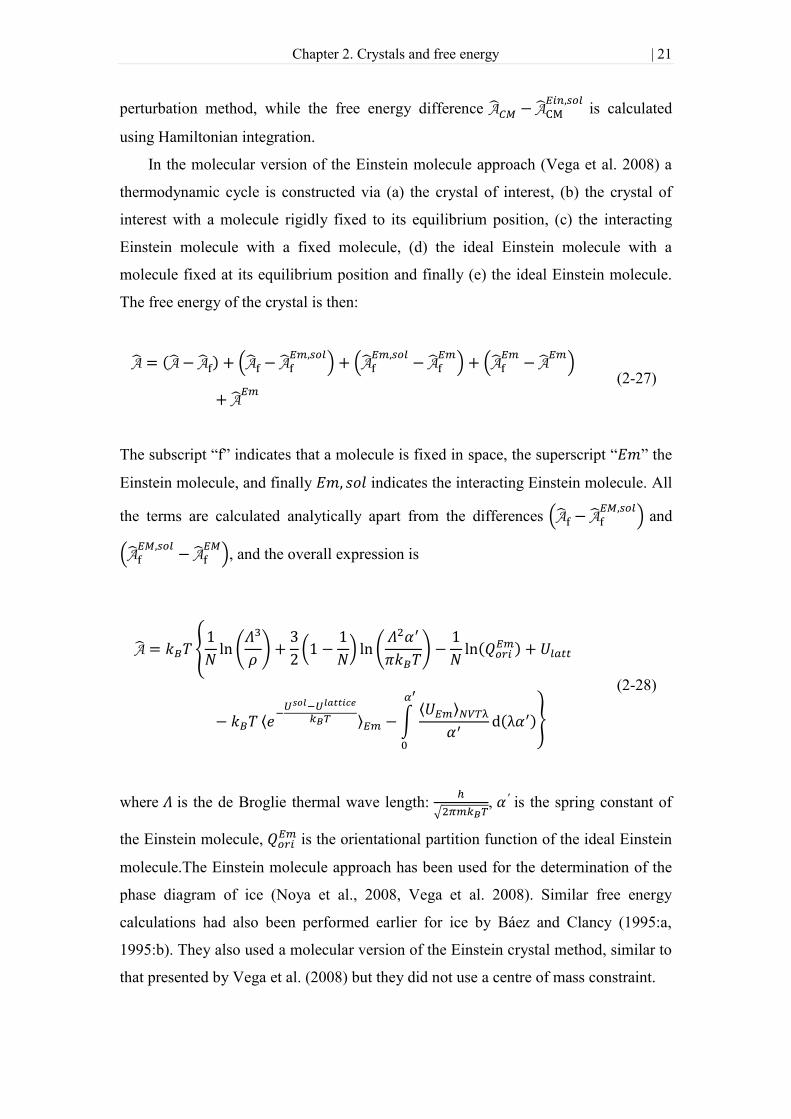
In the molecular version of the Einstein molecule approach (Vega et al. 2008) a
thermodynamic cycle is constructed via (a) the crystal of interest, (b) the crystal of
interest with a molecule rigidly fixed to its equilibrium position, (c) the interacting
Einstein molecule with a fixed molecule, (d) the ideal Einstein molecule with a
molecule fixed at its equilibrium position and finally (e) the ideal Einstein molecule.
The free energy of the crystal is then:
(2-27)
The subscript ― ‖ indicates that a molecule is fixed in space, the superscript ― ‖ the
Einstein molecule, and finally indicates the interacting Einstein molecule. All
the terms are calculated analytically apart from the differences
and
, and the overall expression is
(2-28)
where is the de Broglie thermal wave length:
, is the spring constant of
the Einstein molecule, is the orientational partition function of the ideal Einstein
molecule.The Einstein molecule approach has been used for the determination of the
phase diagram of ice (Noya et al., 2008, Vega et al. 2008). Similar free energy
calculations had also been performed earlier for ice by Báez and Clancy (1995:a,
1995:b). They also used a molecular version of the Einstein crystal method, similar to
that presented by Vega et al. (2008) but they did not use a centre of mass constraint.

Chapter 2. Crystals and free energy | 22
Baele in 2002 proposed the acoustic crystal thermodynamic integration method,
another variation of the Einstein crystal method in which the reference state is the so-
called acoustic crystal, in which the atoms vibrate harmonically and are coupled only
with their nearest neighbours.
A method for the direct calculation of the free energy difference between the
solid and the liquid phases is the constrained λ-integration (Grochola, 2004). A three
stage thermodynamic cycle is employed in which (a) the liquid is transformed into a
weakly attractive fluid, (b) the weakly attractive fluid is constrained to the solid
configuration space via the insertion of Gaussian wells distributed in a lattice, and
finally (c) the Gaussians are turned off, while simultaneously the true potential of the
system is reinstated. The free energy differences between all stages are calculated
using thermodynamic integration along a Hamiltonian path, an approach referred by
Grochola as λ-integration. During the first stage a contraction of the volume is applied
simultaneously with the decrease of the attractive forces. The author clarifies that
although such a decrease in volume is necessary since the solid is denser, it needs not
be done at the first stage. Grochola used this method in conjunction with linear
interpolation in order to determine the solid-liquid coexistence of a truncated and
shifted Lennard-Jones system.
Eike et al. (2005) used slightly modified constrained λ-integration method
together with multiple histogram reweighting and Gibbs-Duhem integration (Kofke,
1993), to determine the solid-liquid coexistence of a Lennard-Jones solid and NaCl.
Eike et al. use the term pseudosupercritical path (PSCP) instead of the constrained λ-
integration, by analogy to the supercritical paths that allow the transformation of the
liquid to the gas without a phase transition to occur. In contrast to Grochola the
reduction of the simulation cell volume is performed during the second stage of the
integration, a choice that is justified by the allowance of more free space for the
particle during the early parts of the second stage. Similar calculations were later
performed for the crystals of triazole and benzene (Eike & Maginn 2006). The
pseudosupercritical path is further modified here and the volume contraction is
performed in a separate stage using integration along an isotherm (equation 2-17).
Using this methodology the melting point and relative thermodynamic stability of the
orthorhombic and monoclinic polymorphs of a salt have also been calculated
(Jayaraman & Maginn, 2007).

Chapter 2. Crystals and free energy | 23
2.4.3. Expanded ensemble methods
A set of methods that have also been used for the calculation of free energy
differences is the so called expanded ensemble methods. Lyubartsev et al. (1992)
proposed a Monte Carlo scheme in which an expanded canonical ensemble is
sampled. The expanded ensemble is a weighted sum of canonical (sub-)ensembles of
the same system but at difference temperatures. The expanded ensemble is sampled in
a single ordinary Monte Carlo simulation, in which additional ―moves‖ are included
so that various temperatures are sampled. In this way the free energy of each
temperature can be obtained with reference to one of them. Other expanded ensemble
techniques exist such as the augmented grand canonical technique of Kaminsky
(1994), or the method of Wilding and Müller (1994) for polymers. Those methods do
not seem appropriate for solids as they rely on the insertion and deletion of molecules.
The lattice-switch method (Bruce et. al., 1997, 2000) is a Monte Carlo technique
that allows direct evaluation of the free energy difference between two crystalline
states. The configuration space of both states is visited in a single simulation. This is
accomplished by Monte Carlo ―moves‖ that involve the switch of the lattice vectors
from those of one crystal to those of the other. When such a move is attempted the
position of the atoms relative to the origin of the unit cell they belong to does not
change. In order for the lattice-switch moves to be accepted multicanonical Monte
Carlo (Berg & Neuhaus T, 1992), a biased Monte Carlo technique, is used. The
method was used for the calculation of the free energy difference between the two
closed packed structures, the face centred cubic (fcc) and the hexagonal closed packed
(hcp).
2.4.4. Other methods
The method of metadynamics (Laio & Parrinello, 2002) can also be used to
estimate the free energy of a crystal (Martoňak et al., 2003). In metadynamics a free
energy basin is explored in a steepest-decent fashion. The system is prevented from
being confined in the basin by a history-dependent term. The history-dependent term
is a superposition of Gaussians accumulated while the procedure evolves. Each
Gaussian is constructed at every step of the algorithm and prevents the system from

Chapter 2. Crystals and free energy | 24
revisiting configurations already visited. In this way all free energy barriers can be
overcome and the hyper-surface is explored. The free energy hyper-surface is then
obtained (within an additive constant) by using the penalizing history term. Although
in principle the free energy can be estimated by metadynamics that is usually not done
(Martoňak et al., 2003). The method has found applications in the study of phase
transitions (Karamertzanis et al. 2008; Raiteri et al., 2005)
Finally the free energy of a solid can be calculated using the method of lattice
dynamics under the so-called harmonic approximation. In this method an analytical
expression is obtained for the free energy of the crystal by approximating its lattice
energy with a quadratic function. The fact that no molecular simulation is required
significantly reduces the computational cost. This is a considerable advantage over the
other methods for the calculation of the free energy, especially in the context crystal
structure prediction where it is necessary to evaluate the free energy of a large number
of structures (of the order of hundreds). The approximation is valid for a restricted
temperature range, but such an approach should nevertheless provide some useful
information on temperature effects. Therefore this method is adopted and a detailed
description follows in the next chapter.

Chapter 3. Lattice dynamics | 25
3. Lattice dynamics
Lattice dynamics is a method that is commonly used for the calculation of the free
energy of a crystal and many other properties. Despite the fact that more accurate an-
harmonic methods are known (Dove, 1993; Ghatak & Kothari, 1972), we will study
lattice dynamics under the widely used harmonic approximation. The advantages of
simplicity and low computational cost of the harmonic approximation outclass the
slightly improved accuracy of the an-harmonic approach. Another widely used option
is the quasi-harmonic approximation, in which the local minimum of the free energy
is obtained.
In order to obtain an analytical solution for the Newton‘s equations of motion a
quadratic approximation of the true potential of the crystal is adopted. In this way the
problem is reformulated into an eigenvalue problem, the solution of which allows the
calculation of the frequencies of atomic vibrations. This approach has its roots in the
work of Born and von Kàrmàn (1912, 1913). Given this information an analytical
expression for the free energy can be obtained. A detailed description of the theory of
harmonic and quasi-harmonic approximations follows in subsequent sections. The
chapter ends with a brief survey of various applications of the method that can be
found in the literature.
3.1. Harmonic approximation
We assume that the crystal has unit cells in the three directions, where is
sufficiently large that the crystal can be considered infinite, i.e. . The unit cell
contains molecules. Indices , and , are used to
enumerate the molecules in the unit cell. The number of atoms in molecules and
are denoted by and , respectively. Note that any two molecules in the unit

Chapter 3. Lattice dynamics | 26
cell can have different numbers of atoms. The indices , and
, to enumerate the atoms in molecules and , respectively. Given an
arbitrarily chosen unit cell (the reference unit cell), a set of vectors , , can be
defined such that exactly one vector corresponds to every unit cell. This vector
indicates the translation operation that allows the coordinates of an arbitrary point in
an arbitrary unit cell to be obtained from those of the same point in the reference unit
cells. Thus the element of a given vector l are the integer numbers of lattice vectors
that must be added to an arbitrary point in the reference unit cell to obtain the
completely equivalent point in the unit cell to which the vector corresponds. It is
obvious that the reference unit cell has l=(0,0,0) and that there are vectors l. The
configuration of the crystal is defined by means of the atomic coordinates:
where is the position vector of the ith
atom of the Ith
molecule of the lth unit cell.
can also be expressed as the sum of the position vector of the origin of the lth
unit
cell, , and the position vector of atom Ii with reference to the origin of the unit cell,
:
The lattice energy, , of the crystal is a function of the configuration, U=U( ),
and can be approximated using a Taylor series expansion around any reference point
:
(3-1)

Chapter 3. Lattice dynamics | 27
where H.O.T. denotes the higher-order terms. The Taylor expansion of equation (3-1)
is valid for any expansion point . The solution of the lattice dynamics equations
within the harmonic approximation requires the expansion point to be a minimum
with respect to the lattice energy (equilibrium position). At any such point, the forces
on all atoms vanish:
(3-2)
In addition, the higher-order terms of equation (3-1) are also ignored and the lattice
energy becomes a quadratic function of the displacement:
(3-3)
In equation (3-3), is the displacement of atom Ii in lth
unit cell from its
equilibrium position: .
The vibration of atoms in the crystal can be modeled with Newton‘s equations
of motion. By substituting equation (3-3) into (3-2) and considering that the
derivatives of the lattice energy with respect to atomic positions are equal to its
derivatives with respect to the displacement, Newton‘s equations become:
(3-4)
where is the mass of the atom characterized by the indices , and the symbol
followed by one or more indices implies that each of the indices takes all the
permissible values.
The solution of equations (3-4), , has the general form of a harmonic wave:
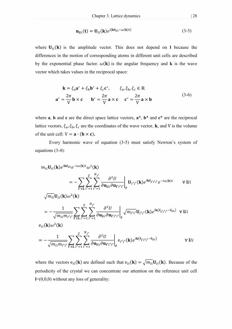
Chapter 3. Lattice dynamics | 28
(3-5)
where is the amplitude vector. This does not depend on l because the
differences in the motion of corresponding atoms in different unit cells are described
by the exponential phase factor. is the angular frequency and k is the wave
vector which takes values in the reciprocal space:
(3-6)
where a, b and c are the direct space lattice vectors, a*, b* and c* are the reciprocal
lattice vectors, are the coordinates of the wave vector, , and is the volume
of the unit cell: .
Every harmonic wave of equation (3-5) must satisfy Newton‘s system of
equations (3-4):
where the vectors are defined such that . Because of the
periodicity of the crystal we can concentrate our attention on the reference unit cell
l=(0,0,0) without any loss of generality:

Chapter 3. Lattice dynamics | 29
(3-7)
We define the polarization vectors and the
symmetrical dynamical matrix:
(3-8)
containing an array of blocks, each defined as:
(3-9)
Then equation (3-7) can be written as:
(3-10)
This last equation describes an eigenvalue problem. Because the elements of
the dynamical matrix are matrices, matrix is a matrix. In addition
the elements of the matrix are matrices. Thus each polarization
vector has elements. As a result there are eigenvalues, and
eigenvectors, for the eigenvalue problem defined in equation (3-10).
From equation (3-10), it can be seen that the squares of the angular
frequencies (and hence the vibrational frequencies
) and the polarization vectors (up to a multiplication constant) can be
obtained by diagonalizing the dynamical matrix . It can be seen readily from
equation (3-9) that the dynamical matrix is Hermitian as and therefore it
has real eigenvalues (positive or negative). Negative eigenvalues of the dynamical
matrix imply that the structure is unstable.

Chapter 3. Lattice dynamics | 30
It is important to note that if a harmonic wave such as that of equation (3-5) were
propagating in a continuous medium, then for every wave vector k there would be
infinite number of compatible angular frequencies . The discontinuity of the
crystal implicitly results in the restriction of the number of compatible wave vectors,
so that only such vectors exist. The 3N corresponding frequencies are those which
allow the compatibility of the harmonic wave equation (3-5) with the equations
of motion (3-4).
It is interesting to point out that the dynamical matrix is closely related to the
force constant matrix use by Tan et al. (2010). The dynamical matrix is the mass
weighted force constant matrix of the derivative based harmonic system (section
2.4.1).
3.2. Assumptions and necessary conditions
It is worth stressing that the lattice energy to which we refer in section 3.1
differs from the lattice energy of a single unit cell which is calculated and
minimized in the lattice energy minimisation algorithms for crystal structure
prediction in that is the lattice energy of the whole crystal.
The use of the whole crystal rather than the unit cell is necessary for the
calculation of second derivatives in equation (3-9), which must be computed without
imposing periodicity during differentiation, because the derivative
involves the displacement of atom in the reference unit cell (cell 0) and the atom
in unit cell l only, i.e., with all other atoms fixed at their equilibrium positions.
These gradients differ from the gradients of that are used in lattice energy
minimisation algorithms. When calculating the gradients of with respect to the
atomic positions of any atom in the reference unit cell, all its periodic images are
perturbed. This is because in lattice energy minimisation algorithms the periodic
structure with minimum energy is sought.
In principle, the conditions implied by equation (3-2) should be true for all the
structures on which lattice dynamics calculation are performed. Unfortunately it is not
possible to check directly if this condition is fulfilled because (a) the lattice energy
cannot be calculated since an infinite summation is involved, and (b) condition (3-2)

Chapter 3. Lattice dynamics | 31
describes an infinite number of gradients that need to be calculated. The validity of
conditions (3-2) is checked in an implicit way, using the (periodic) gradients of .
Three further assumptions are adopted, in keeping with many crystal modeling
studies:
1. Our crystal extends from minus infinity to infinity in every direction (
). This assumption is justified by the fact that we are interested in bulk
properties and consequently we want to avoid surface effects.
2. The crystal is perfect (i.e. there are no defects) and periodic in every direction.
3. The cyclic (or periodic) boundary condition (Born & Huang, 1954; Dove,
1993; Ghatak & Kothari, 1972), due to Born and von Kàrmàn (1912, 1913) is
adopted.
Under the first two assumptions, condition (3-2) is completely equivalent to the
condition:
(3-11)
It is intuitively understood that if the number of unit cells ―approaches‖ infinity and
the crystal is perfect and fully periodic, the environment is the same around every unit
cell. As a result, the energy of every atom in a given unit cell will be the same as that
of the corresponding atom in every other unit cell. The last assumption (cyclic
boundary condition) has no immediate impact, but it will be useful later in the
discussion.
Although condition (3-11) is necessary and sufficient for equation (3-2) to be
true, a minimization of the lattice energy with respect to the atomic positions and the
lattice unit vectors is always performed before every lattice dynamics calculation. At
the lattice energy minimum, in addition to condition (3-11), the following condition is
true:
(3-12)
where R is a matrix whose columns are the lattice vectors of the crystal .
Although this condition is not necessary for lattice dynamics calculation to be

Chapter 3. Lattice dynamics | 32
performed, in practice it holds for every structure for which such a calculation is
carried out. This is because the result of a minimisation which is performed solely
with respect to the atomic position is a structure without physical meaning.
Once the minimum lattice energy structure is obtained then the second
derivatives of interest,
, are calculated and the lattice dynamics calculation
is performed.
3.3. The permissible wave vectors
The translational symmetry of the crystal allows a description of the crystal by means
of the formalism of group theory (McWeeny, 1963). The set of all possible
translations in the crystal, i.e., mappings of the form:
where
(3-13)
form a group. Under the Born and von Kàrmàn cyclic boundary condition adopted
here (see section 3.2):
, (3-14)
the sub-group of translations becomes a cyclic group, whose representations are those
of any ordinary cyclic group (McWeeny, 1963):
(3-15)
In equation (3-15) each combination of the indices ξ
, ξ
and ξ
describes a
representation of the (cyclic) sub-group of translations. In this way equation (3-15)
provides representations of the translation sub-group of the crystal. In
addition, ξ ξ ξ represent non-normalized coordinates of the wave vector, .

Chapter 3. Lattice dynamics | 33
The major conclusion from equation (3-15) is that there are wave vectors
permitted for the crystal, i.e., the number of wave vectors is the same as the number of
unit cells in the crystal. These have (positive) coordinates :
(3-16)
This suggests that it is sufficient to restrict the wave vector, , to the ―first‖ unit cell
of the reciprocal lattice. If a wave vector is related by a reciprocal lattice vector, ,
to a wave vector , , in the first reciprocal unit cell:
where
then the wave vector is such that (a) identical motion is described by equation
(3-5), (b) identical solutions are obtained to the eigenvalue problem of equation (3-10)
and (c) in the language of group theory, an indistinguishable representation is
obtained. It is easy to prove that is equal to , where is an integer, and
consequently:
(3-17)
A discussion of the issue of permissible wave vector values and their effect on the
atomic vibrations can be found in Born & Huang (1954), Dove (1993, 2003) and
Ghatak & Kothari (1972). A formal and robust mathematical discussion of this issue
based on arguments of group theory can be found in McWeeny (1963).
In the limit of an infinite number of unit cells (see section 3.2) the upper bound
for the wave vector coordinates is
This suggests that restricting the wave vector to the reciprocal lattice unit cell ,i.e.,
, would produce sufficient information for the complete study of
the dynamical properties of the crystal.
Sometimes, instead of restricting the wave vector to a unit cell of the reciprocal
lattice it is confined to the first Brillouin zone (Born & Huang, 1954; Dove, 1993,

Chapter 3. Lattice dynamics | 34
2003; Ghatak & Kothari, 1972), defined as a section of the reciprocal space that has a
volume equal to that of a reciprocal lattice unit cell, therefore containing all the
necessary information. A discussion of the construction of the various Brillouin zones
can be found in Brillouin (1953). In this thesis calculations are performed within a
reciprocal lattice unit cell rather than in the Brillouin zone. The value of the free
energy, which is a scalar quantity, is independent of the choice of the period to be
studied, and therefore the easiest choice in terms of implementation is adopted.
3.4. Normal modes & dispersion curves
Each of the solutions of the eigenvalue problem (3-10), and
describes a mode of vibration of the crystal. The quantities
(3-18)
are known as normal modes or normal mode coordinates. The normal modes can be
used as generalized degrees of freedom (―coordinates‖) by means of which the system
can be described, i.e. the Hamiltonian can by expressed (Born & Huang, 1954; Dove,
1993; Ghatak & Kothari, 1972). In this form of the Hamiltonian each of the terms of
the potential energy is a function of the square of one of the normal modes:
(3-19)
The Cartesian form (equation 3-3) of the potential energy, on the other hand,
comprises terms coupling the various degrees of freedom. Equation (3-18) is the
complex form of a harmonic wave, therefore it is usually said that the crystal can be
analyzed as a set of harmonic waves independent with each other.
The number of normal modes is equal to the number of degrees of freedom of the
crystal in its Cartesian representation. The normal modes are connected to the
Cartesian displacements of the atoms via a linear transformation:

Chapter 3. Lattice dynamics | 35
(3-20)
Equations (3-20) are intuitively understood as an analysis of the true motion of the
atoms in the crystal into a set of harmonic waves, or that the true motion of the atoms
in the crystal is the superposition of all the harmonic waves that are allowed to
propagate in the crystal.
The plot of the frequency of each mode of vibration as function of the
wave vector is called the dispersion curve and the curve associated with each mode
is known as branch of the dispersion curve. In general there are modes of vibration
whose frequency vanish at the Γ-point of the Brillouin zone ( ), i.e.
. These modes are known as acoustic modes. The frequency
of all the other modes has a non-zero value for , and are known as optical
modes. Another distinction of the modes can be made when the crystal consists of
polyatomic entities, such as molecules or polyatomic ions. If there are molecules in
the unit cell and atoms, then out of the branches of the dispersion curve, the
lowest frequency represent the so-called external modes, and correspond to the
motion of the polyatomic entities as rigid objects. The remaining modes are
the so-called internal modes. The 3 acoustic modes belong to the set of external
modes.
More details on the various types of modes can be found in Born & Huang
(1954), Dove (1993, 2003) and Ghatak & Kothari (1972). The formulation of the
calculation of the external modes has been presented by Venkataraman & Sahni
(1970) and Pawley (1972).
3.5. Calculation of the free energy
In order to calculate the Helmholtz free energy of the crystal a quantum
description of the energy states of the system is adopted. The quanta associated with
each normal mode are known as phonons in analogy with the photons of the
electromagnetic theory of light. Each normal mode is described quantum

Chapter 3. Lattice dynamics | 36
mechanically via the quantum harmonic oscillator equations. This result can be
obtained more formally by applying the commutation relations between the normal
mode coordinates and the corresponding momenta, as is done, for example, in Ghatak
& Kothari (1972). The total vibrational energy of the crystal is then the sum of the
energies of the various independent waves.
Within the quantum mechanical framework the energy states of a harmonic
oscillator whose frequency is are separated by an energy gap of :
(3-21)
where is Planck‘s constant and η is the quantum number. It is important to note that
the ground state of the quantum harmonic oscillator, which corresponds to , is
equal to
and not equal to zero.
Equation (3-21) can be used to derive a description of each mode of vibration
of the crystal (i.e. each branch of the dispersion curve), as follows:
(3-22)
This equation describes the energy states of the th mode of vibration for a given
value of the wave vector, k.
Statistical mechanics can be used to formulate an expression for the Helmholtz
free energy of the crystal. This is done in two steps:
1. Initially the canonical partition function is constructed.
2. The free energy is formulated, employing the general equation
The definition of the partition function of the canonical ensemble is (Allen
& Tildesley, 1987; Frenkel & Smit, 2002; Hill, 1986; McQuarrie, 2000):
(3-23)

Chapter 3. Lattice dynamics | 37
where the summation is over all energy states of the system , enumerated by the
index . The energy of the crystal is the sum of the static and vibrational
parts. The vibrational part results from the superposition of all possible waves
propagating along the crystal:
(3-24)
The partition function is then given by:
(3-25)
When exploiting the properties of the exponential and the distributive property, the
partition function takes the form:
(3-26)
Finally using the series expansion:
(3-27)
we can convert the last summation in equation (3-26) so that :

Chapter 3. Lattice dynamics | 38
(3-28)
The free energy is then obtained by substitution of the partition function expression in
the well-known formula:
, (3-29)
giving as a final expression:
(3-30)
The last expression for the Helmholtz free energy (equation 3-30) often appears in the
literature in other forms (Kopsias & Theodorou, 1998; Westacott & Rodge, 1996,
1998 ):
(3-31)
where is related to Planck‘s constant
. Note that these expressions for the
free energy of the harmonic oscillator differ from the expression used by Tan et al.
(2010) and described in section 2.4.1 (equation (2-15)). This is because here we are
using the quantum description for the harmonic oscillator while equation (2-15)
corresponds to the partition function of the classical harmonic oscillator.
Equation (3-31) is a general equation derived without any approximation other
that the quadratic expansion of the lattice energy and is true for every perfect crystal.
Of course the number of wave vectors propagating along the crystal is infinite since it

Chapter 3. Lattice dynamics | 39
is equal to the number of the unit cells in the crystal (see section 3.4), which we have
assumed to tend to infinity, and therefore it is not possible to evaluate it directly. For
this reason a number of alternative expressions can be used to evaluate the Helmholtz
free energy.
If equation (3-30) is divided by we obtain an expression for the free
energy that involves an average over all possible wave vectors:
(3-32)
where is the Helmholtz free energy per unit cell of the crystal and indicates
an average over all possible wave vectors.
As was shown in section 3.3, the feasible wave vectors are infinite, evenly-
distributed wave vectors in the unit cube , therefore the average
over discrete vectors described in equation (3-32) can be expressed as an integral:
(3-33)
If the free energy of interest is the Gibbs free energy, , we need to formulate the
grand canonical partition function . This is done in a completely analogous way
to the derivation of equation (3-28) and one obtains:
(3-34)
The Gibbs free energy is then obtained using :

Chapter 3. Lattice dynamics | 40
(3-35)
where is the Gibbs free energy per unit cell and is the volume per unit cell.
3.6. The density of vibrational states
The density of vibrational states, widely denoted by , is a comprehensive way
to characterize the dynamical state of the system. It is also referred to in the literature
as vibrational spectrum or normal mode density. The density of states is defined as
follows (Ghatak & Kothari, 1972):
“The frequency distribution function is the number of vibrational modes per
unit frequency around .”
In mathematical terms, in the limit of an infinite crystal lattice, is given by (Born
& Huang, 1954):
(3-36)
Here is the volume of the reciprocal unit cell given by . It is
easy to prove that
As a result is the number of modes per unit volume lying between and
. The density of states has the property:
(3-37)
Using the density of states, the Helmholtz free energy can be written as:

Chapter 3. Lattice dynamics | 41
(3-38)
and the Gibbs free energy as:
(3-39)
There are a number of methods for approximating the density of states (Blackman,
1937; Gilat & Raubenheimer, 1966; Houston, 1948; Montroll, 1942) that are
summarized in Born & Huang (1954), De Launay (1956) and Ghatak & Kothari
(1972). One can even find analytical expressions for simple systems, such as a one-
dimensional crystal of equally spaced identical atoms (Ghatak & Kothari, 1972). The
capabilities of modern computers allow the calculation of for complex systems
directly via sampling, using its definition (equation 3-36).
In a sampling approach, given a sufficiently large number of wave vectors
, the frequencies of atomic vibrations are calculated by solution of the
eigenvalue problem given by equation (3-10). Then a ―binning‖ procedure is applied:
(3-40)
is an upper bound for the frequencies of the crystal and
is the number of
intervals (―bins‖) in which the domain is divided.
3.7. Evaluation of the free energy expression
The expression for the free energy (equation 3-33 or 3-35) can be evaluated in
many ways. A rather coarse categorization of available methods can be made on the

Chapter 3. Lattice dynamics | 42
basis of the following classes: ―approximate” methods, non-symmetry based
methods, symmetry-based methods and quadrature methods.
There are two widely known approximate methods for the evaluation of the free
energy, the Einstein approximation (Dove, 1993; De Launay, 1956) and the Debye
approximation (Dove, 1993; Wallace, 1972; De Launay, 1956). Einstein (1907) first
used quantum mechanics to describe the vibrations of atoms within a crystal. He
assumed that the atoms in the crystal do not interact, and that they all vibrate
harmonically and independently with the same frequency. Under those assumptions
he obtained a simple analytical expression for the free energy and every other
property of the crystal. The frequency of atomic vibrations is usually fitted when
applying this approach. On the other hand, Debye ignored the optical modes and
considered only acoustic modes which were assumed to be linear and to have the
same slope. He assumed an upper bound for the frequencies of the vibrations,
obtaining a quadratic expression for the density of the vibrational frequencies
(equation 3-36), which could then be used to evaluate the free energy.
Various methods can be found in literature in which the wave vectors are
sampled in the first Brillouin zone, the density of states is then constructed on this
basis and finally the free energy is evaluated using equations (3-38) and (3-39). We
refer to these methods as non-symmetry based methods. For example, van Eijk (2001)
sampled wave vectors randomly in the primitive reciprocal lattice unit cell, in crystals
of glycerol and glycol. He used 50 wave vectors to ensure the density of states
converges. One can also construct a grid in the Brillouin zone which can be even
(Dove, 1993) or uneven (Filippini et al., 1976). The main advantage of these methods
is their simplicity, while their main disadvantage is the limited efficiency.
One can also find in the literature a number of methods that take advantage of
the symmetry properties of the crystal in order to improve the efficiency of Brillouin
zone sampling. We refer to these methods as symmetry-based methods. Bladereschi
(1972) proposed a method for the identification of a unique point in the Brillouin zone
that has the property that the value of any periodic function of the wave vector at this
point is the same as the average of that function over the Brillouin zone. Such a point
may be difficult, if not impossible, to identify, and for this reason another method was
proposed (Chadi & Cohen, 1973) for the identification of an arbitrarily small number
of points in the Brillouin zone, chosen such that the weighted sum of the value of the
function at these points is a good approximation of the mean value of the function.

Chapter 3. Lattice dynamics | 43
Other methods that take advantage of the symmetry of the crystal include the
Monkhorst & Pack (1976) method, and the ―special directions‖ method (Bansil, 1975;
Prasad & Bansil, 1980). Although these methods allow the efficient evaluation of the
free energy, their applicability to crystals of arbitrary symmetry is questionable.
Finally the triple integral of equation (3-33) can be evaluated using any of the
numerical analysis methods that are suitable for this type of integral. We adopt this
approach here, and the Gauss-Legendre quadrature is chosen for the evaluation of the
free energy.
The Gauss-Legendre method is a special case of the Gaussian quadrature class of
methods. In Gaussian quadrature, a weighted integral of the function f(x) between
limits and is approximated as:
(3-41)
where is a weighting function, the ‘s, which are elements of the N-
dimensional vector x, are known as the abscissae or nodes of the quadrature method,
are the coefficients of the method and is an natural number
The various Gaussian quadrature methods, such as Gauss-Jacobi or Gauss-
Chebyshev differ in and in the way the coefficients and the abscissae are
chosen. In the Gauss-Legendre quadrature the weighting function is constant and
equal to one and the general form of the integral is:
(3-42)
The coefficients in the Gauss-Legendre quadrature method for a specific are the
roots of the th order Legendre polynomial defined as:
(3-43)

Chapter 3. Lattice dynamics | 44
As soon as the roots of the Legendre polynomial have been found,
the coefficient of the quadrature formula associated with each root can be calculated
using the equation:
(3-44)
where is the gradient of at
and is the leading coefficient of the
normalized th order Legendre polynomial:
This coefficient can be proven that are equal to:
(3-45)
If the limits of the integration are different from and , as in equation (3-33), then
the same abscissae and coefficients can be used, but the quadrature formula must be
modified as follows:
(3-46)
Finally, the extension of the quadrature formula in the case of multiple integrals is
straight forward:
(3-47)

Chapter 3. Lattice dynamics | 45
In Table 3-1 the abscissae and coefficients of the Gauss-Legendre quadrature for
different values of the number of nodes are summarized. Details about the method and
extended tables with abscissae and coefficients can be found in literature
(Abramowitz & Stegun, 1972; Krylov, 1962; Stroud, 1966).
3.8. The quasi-harmonic approximation
Within the harmonic approximation, the minimum of the free energy coincides
with the minimum of the lattice energy function. This is readily understood if we
differentiate the expression for the free energy (equation 3-30):
(3-48)
where is any variable of the crystal structure. The derivative can equivalently be
written in terms of the derivative of the corresponding eigenvalue of the dynamical
matrix
(3-49)
N ( Coefficient , Abscissa(s) )
1
2
3
4
Table 3-1 The coefficients and corresponding abscissas for Gauss-Legendre
quadrature. The density of sampling is limited to four nodes per direction.

Chapter 3. Lattice dynamics | 46
Using first-order perturbation theory, it can be proven that the derivative of each
eigenvalue of the dynamical matrix is given by (Gale, 1998; Gale & Rohl, 2003;
Kantorovich 1995; Taylor, 1997, 1998):
(3-50)
The formalism of the harmonic approximation is built on the assumption that the
potential is a quadratic function and that the dynamical matrix is essentially a sum of
the second derivatives (equation 3-9), so that the derivative of the dynamical matrix is
related to the third derivative of the lattice energy. For a quadratic lattice energy
function, this derivative is zero. Therefore the minimum of the free energy within the
harmonic approximation coincides with the lattice energy minimum. In addition, any
attempt to minimize the free energy derived under the harmonic approximation by
moving the system from its minimum lattice energy configuration would violate the
necessary condition on which all the formalism has been built (equation 3-2).
In spite of this, it is common practice to minimize a free energy obtained using the
harmonic approximation. This is done by calculating the derivative in equation (3-50)
using the third derivative of the true lattice energy function, . This derivative had
been truncated from the Taylor expansion approximation of (equation 3-1) in
order to simplify the solution of lattice dynamics in the form of the eigenvalue
problem (3-10). When reinstating this derivative, the necessary conditions (3-2) no
longer hold. For these reasons, minimization schemes that are performed using
equations (3-49) and (3-50) are said to adopt a quasi-harmonic approximation (Dove,
1993).
It should be also stressed that in the literature (Gale, 1998; Gale & Rohl, 2003;
Kantorovich 1995; Taylor et al., 1997, 1998), it is common practice to perform a free
energy minimization using a quasi-Newton algorithm, such as the Broyden-Fletcher
Goldfarb-Shano (BFGS) algorithm (Press et al., 1986), because it does not require the
calculation of the Hessian, which would involve the calculation of the second
derivative of the dynamical matrix, and hence the fourth derivative of the lattice
energy. Impractically long CPU time would be necessary for a full Newton algorithm,
rendering the calculation infeasible.

Chapter 3. Lattice dynamics | 47
3.9. Applications of lattice dynamics
Lattice dynamics has been used for many years (Born & von Kàrmàn, 1912,
1913), mainly under the harmonic and quasi-harmonic approximations, in several
applications and on various systems, including organic compounds such as
naphthalene and inorganic systems such as ArO. In this section, we provide an
overview of some of the key applications of lattice dynamics, to illustrate the breadth
of systems studied, and the range of properties that have been investigated within this
framework. It should be stressed that this is only a brief survey of the literature which
is by no means exhaustive.
3.9.1. Inorganic crystals
Rare gas crystals have provided a useful testing ground for lattice dynamics.
Using the Lennard-Jones potential (Kaplan, 2006; Lennard-Jones, 1937) for modeling
repulsion and dispersion interactions De Wette and co-workers (1971) derived phonon
dispersion curves of the Lennard-Jones system in reduced units. Under the quasi-
harmonic approximation they calculated the specific heat and thermal expansion of Ar
as a function of temperature. The necessary lattice sums in this study were calculated
using tabulated values found in the literature (Misra, 1940). Recently lattice dynamic
calculations were adopted to study compressed rare gas crystals (Ne, Ar etc.). The
calculations were performed within the framework of the Tolpygo model using ab-
initio potentials (Horbenko et al., 2007, Troitskaya et al., 2005, 2009).
Inorganic solids, for which there is a wealth of data, have also been the subject of
numerous investigations with lattice dynamics. One of the early applications of the
harmonic theory of lattice dynamics is the calculation of the phonon frequencies and
density of states of NaCl, in the pioneering work of Kellermann (1940). This
information was later used for the calculation of the specific heat of sodium chloride
(Kellermann, 1941). In contrast to Kellermann, who assumed ―rigid ions‖, Caldwell
& Klein (1967) used the ―shell model‖ to include the effect of polarizability in the
calculation of the phonon dispersion curves and the density of states of NaCl. The
―shell model‖, originally proposed by Dick & Overhauser (1958), had earlier been

Chapter 3. Lattice dynamics | 48
extended and applied to NaI and KBr crystals (Cowley et al., 1963; Woods et al.,
1960, 1963). Another model aiming to model the deformation of the electronic cloud
is the ―deformation-dipole‖ (DD) model (Karo & Hardy, 1966). The DD model has
been shown by Karo and Harding to give very accurate dispersion curves, density of
states, and heat capacity of NaCl. In all these studies, the calculations were performed
using the experimentally-determined crystal structure. Permanent electrostatic
interactions were usually calculated using the Madelung treatment (Madelung, 1918)
while repulsion interactions were calculated considering interactions up to second
neighbors only. A variation on this type of model is the so-called ―van der Waals
three-body force shell model‖ (VTSM), where three-body and dispersion interactions
are also included in the calculations. This has been applied to lattice dynamical
calculations of thallous bromide, TlBr, (Tiwari et al., 2009, 2010), thallous chloride,
TlCl, (Tiwari et al., 2010) and potassium bromide, KBr, (Srivastava et al., 2010), for
which various properties related to the dynamics (such as optical properties, dielectric
constant) are available. Jaswal and co-workers have obtained phonon dispersion
curves in crystals of lithium deuteride, LiD, (Jaswal & Dilly, 1977:a), magnesium
oxide, MgO, (Jaswal & Dilly, 1977:b), zinc sulfide, ZnS, (Jaswal, 1978:a) and copper
chloride, CuCl, (Jaswal, 1978:b), using the so called ―deformable-ion‖ model, a
generalization of the shell model and the deformation-dipole based on Tolpygo‘s
theory.
More complex problems can also be tackled using the method of lattice dynamics.
Self-diffusion coefficients in MgO crystals that have a defect, a system of geological
interest since it is abundant in the Earth‘s mantle, have been calculated under the
harmonic approximation (Vočadlo et al., 1995). The shell model and the Buckingham
potential were used for modeling inter-atomic interactions. The thermal properties and
elastic properties of calcite (CaCO3), a system composed of polyatomic ions, as a
function of temperature have also been studied using the quasi-harmonic
approximation (Pavese et al., 1996). Electrostatic interactions were modeled using
point charges and the shell model was used for modeling the polarizability of the
oxygen atom. The repulsive interactions were calculated using an exponential pair
potential, while dispersion interactions were included only for the O—O interaction.
The deviations from the ideal planar conformation for the [CO3]-2
ion were modeled
using an empirical potential. Many other studies can be found in the literature such as

Chapter 3. Lattice dynamics | 49
normal mode analysis in SiO4 (Patel et.al., 1991) and in Mg3Al2Si3O12, a commonly
used gemstone also known as ―pyrope garnet‖ (Chaplin et al., 1998).
3.9.2. Organic molecular crystals
The harmonic approximation method has also been applied to organic crystals.
The hexamine crystal (IUPAC name: 1,3,5,7-Tetraazatricyclo[3.3.1.13,7
]decane, with
chemical formula (CH2)6N4) is one of the first organic molecular systems to have
been studied (Cochran & Pawley 1964; Rafizadeh & Yip, 1970). Hexamine is used as
a hardening additive to resins. In these early works, the external modes of the
dispersion curves were derived based on rigid body models. The parameters of the
models were fitted to experimental spectroscopic data. The phase transitions between
the α- and β- forms of p-dichlorobenzene (C6H4Cl2) and those of 1,2,4,5-
tetrachlorobenzene (C6H2Cl4) were the subject of another early study (Bonadeo et al.,
1978). In this work, the lattice dynamics equations were solved using the harmonic
approximation and adopting a rigid-body formalism, and therefore ignoring internal
modes. No electrostatic contributions were considered and the only inter-atomic
interactions considered were of the Buckingham type. The evaluation of the free
energy expression was carried out within the Debye approximation for the acoustic
modes and the Einstein approximation for the optical modes. The method failed to
identify the α- to β- transition in the case of p-dichlorobenzene. Although no phase
transition was identified, the free energy between the two polymorphs was found to be
very small for the whole temperature range studied. A justification put forward by the
authors for this result is the fact that each of the polymorphs can crystallize as a
metastable structure (depending on the experimental conditions) in the temperature
region in which the other polymorph is stable (Ghelfenstein & Szwarc; 1971). This
result suggests that the real free energy difference between the two polymorphs must
be very small. In the case of 1,2,4,5-tetrachlorobenzene, a stability shift is identified at
200 K, surprisingly close to the experimental transition temperature (188±2K)
reported by Herbstein (1965).
A much more sophisticated model was used for frequency calculations for the
experimentally-determined crystals of ammonia (NH3) and deuterated ammonia
(ND3) (Righini et al., 1978). The authors calculated the frequencies of the external

Chapter 3. Lattice dynamics | 50
modes of vibration at the Γ-point, using the Buckingham potential for the calculation
of the repulsion-dispersion interactions. The electrostatic interactions were modeled
using molecular multipole moments up to fourth order of interaction (Neto et al.,
1978). Experimentally-determined dipole and quadrupole moments were used, while
higher moments were determined using ab-initio methods. Later, a full dispersion
curve was calculated (Della Valle et al., 1979).
Different approaches to the modeling of interactions have been investigated in the
application of lattice dynamics to naphthalene (IUPAC name: bicyclo[4.4.0]deca-
1,3,5,7,9-pentene, with chemical formula C10H8). The inclusion of a molecular
quadrupole moment was found to significantly improve the accuracy of the dispersion
curves obtained using lattice dynamics calculations (Righini et al., 1980). Here
calculations had been performed for a crystal in which the lattice variables were those
measured experimentally at 4.7 K, while the molecular conformation and orientation
were those determined at 120 K. Similar dispersion curves had earlier been calculated
without including any electrostatic interactions (Natkaniec et al., 1980). In these
calculations, the authors calculated the phonon frequencies within the quasi-harmonic
approximation by using the experimental unit cell information (at 4.7 K) and by
allowing the molecular orientation to vary. For a similar molecule, anthracene
(C14H10), the external modes and the 4 lowest-energy internal modes have also been
calculated (Dorner et.al., 1982), without consideration of electrostatic interactions.
The dispersion curves of anthracene and naphthalene have also been calculated using
atomic point charges to account for the electrostatic interactions (Criado, 1989). The
effects of temperature and pressure on the crystals of naphthalene have also been
studied (Della Valle et al., 1995). The authors performed their study within the quasi-
harmonic approximation, adopting the Einstein approximation for the optical modes
and the Debye approximation for acoustic modes. A rigid body approximation was
adopted for the calculation of phonon frequencies and no electrostatic interactions
were included in the molecular model.
Ethenetetracarbonitrile, C6N4, (also known as Tetracyanoethylene or TCNE) is
another small rigid molecule that has been widely studied both experimentally and
theoretically because of its exceptional properties (Chetkina & Bel‘skiĭ, 2002) and its
rich phase behavior. TCNE finds various applications such as in superconductors and
magnets. In 1979 a first study of the dynamics of the two polymorphs of TCNE was
published (Luty et al., 1979). A simple ―exp-6‖ potential was used, without any

Chapter 3. Lattice dynamics | 51
explicit accounting of the electrostatic interactions. The lattice energies of both
polymorphs were minimized and frequency calculations were performed under the
harmonic approximation. In later work, the monoclinic phase was studied under strain
using the same model, aiming to ascertain whether lattice dynamics could predict a
phase transition between the two polymorphs (Munn & Luty, 1980). The authors
concluded that since the frequencies associated with certain modes of vibration
become imaginary, it is indeed possible that a phase transition occurs. In both these
studies the lattice dynamics equations were solved for the external modes (within the
rigid-body approximation). The phonon frequencies of TCNE were also calculated by
employing an improved model that includes point charges (Criado, 1990). In this
study, similar calculations were performed for the crystals of 1,1,2,2,-
cyclopropanetetracarbonitrile (C7H2N4), hexamine, pyrimidine (C4H4N2), pyrazine
(C4H4N2) and s-triazine (C3H3N3). The phase diagram for TCNE from 0 K up to 450
K (approaching the normal melting point of 472 K (Funasako et al. 2012; Radomska
& Radomski, 1991)) and up to 4 GPa has also been constructed using harmonic lattice
dynamics (Chaplot, 1987). The model was based on the Buckingham potential and
Coulombic interactions were not considered. The lattice dynamics equations were
solved in a semi-rigid fashion. The approach failed to identify the phase transition
occurring at ambient pressure and the monoclinic polymorph was calculated to be
stable for the whole range of temperatures, contrary to experimental evidence
(Mierzejewski & Chaplot, 1980; Mukhopadhyay et al., 1985; Murgich & Pissanetzky,
1972). A similar study of the relative stability of the cubic and monoclinic forms of
TCNE was carried out very recently in an ab-initio manner (Schatschneider et al.,
2012). A dispersion corrected density function theory (DFT+vdw) methodology
(Tkatchenko & Scheffler, 2009) was used, with a PBE functional. The phase
transition was found to occur at 160 K. This value is lower than both reported
experimentally determined temperatures, 320K in Mierzejewski & Chaplot (1980)
and Mukhopadhyay et al. (1985) and 292 K in Murgich & Pissanetzky (1972).
Day and co-workers (2003) compared the performance of various models of the
repulsion/dispersion and electrostatic interactions in calculations of the harmonic &
quasi-harmonic phonon frequencies at the Γ-point for five small organic molecules
(hexamethylenetetramine, naphthalene, α-glycine (C2H5NO2), imidazole (C3H4N2),
and pyrazine). Calculations were performed under the rigid body assumption. It was
found that both the model for the repulsion/dispersion interactions and the model for

Chapter 3. Lattice dynamics | 52
the electrostatics can have a significant effect on the calculated phonon frequencies.
Smaller differences in the quasi-harmonic approximation phonon frequencies revealed
that the source of error in the harmonic approximation could be partly attributed to the
differences in the relaxed structures. Similar calculations have also been performed
for 5-auzouracil (Gray et al., 2004). A comparison with phonon frequencies obtained
using molecular dynamics simulations showed only minor deviations from those
obtained by lattice dynamics under harmonic and quasi-harmonic approximation for
5-auzouracil and imidazole (Gray et al., 2004)
The Local Harmonic (LH) method of LeSar et al. (1989) is a further simplified
variation of the harmonic approximation. In the LH method all the inter-atomic
coupling system is neglected, by approximating the dynamical matrix by a
block diagonal matrix, i.e., by equating the elements that describe the coupling of the
motion of different atoms to zero. This approach has been used within a free energy
minimization algorithm for the calculation of the free energy of a perfect copper
crystal, and the free energy of a copper crystal with a defect. The result was found to
be in good agreement with the result obtained via Frenkel & Ladd‘s thermodynamic
integration method (see section 2.4). Similar calculations with the LH model have
been performed to obtain the boundary free energy of Au (Najafabadi et al., 1991:a)
or Ni-Cu alloys (Najafabadi et al., 1991:b).
Sutton (1989) studied gold grain boundaries in a different way. A second moment
approximation was adopted for the local phonon density of states, and approximate
expressions were obtained for the free energy gradients. The second moment
approximation has also been used for calculations on alloys, with a slightly modified
expression for the free energy gradients (Sutton et al., 1992).
A similar methodology has been used for the study of complex hydrate systems.
The free energies of hexagonal ice and of the methane hydrate with hexagonal ice
were minimized within the ―local molecular harmonic model‖ (LMHM) (Westacott &
Rodger, 1996). The LMHM method is a generalization of the LH method that was
first presented by LeSar et al. (1989). In the LMHM, all the elements describing the
coupling of atoms that do not belong to the same molecule are assumed to be zero.
The water molecule was modeled using the SPC model (Berendsen et al., 1981) while
a coarse-grained model was adopted for methane, which was represented by a single
Lennard-Jones sphere. The minimizations were performed using numerical gradients,
and the phonon frequencies were assumed to have no dispersion, i.e. only the zero
Chapter 3. Lattice dynamics | 53
reciprocal space vector (Γ-point) was sampled for the evaluation of the free energy
expression. Westacott and Rodger investigated the three-phase equilibria between
methane hydrate, methane gas and ice and obtained results in good agreement with
experimental data for the equilibrium pressure at 270 K and 17% (mol) methane in the
hydrate phase. The authors have also used similar models and the LMHM method for
the determination of critical nuclei for crystallization for methane hydrates (Westacott
& Rodger, 1998).
The quasi-harmonic approximation has also been used to study the amorphous
state of a Lennard-Jones system (Kopsias & Theodorou, 1998). Various potential
energy minima in the amorphous system hyper-surface are identified, by rapid
decrease of the temperature in a molecular dynamics simulation, followed by constant
volume steepest decent potential energy minimization. The free energy minimum is
then obtained by free energy minimization, which is performed under constant
pressure and temperature within the quasi-harmonic approximation. Elementary
transitions are then identified among the minima and the rate constant associated with
the transition from one minimum to another are calculated based on the
multidimensional transition state theory.
Lattice dynamics calculations have also been used to assess the effect of
temperature on the result of a crystal structure prediction study (van Eijk, 2001). van
Eijk calculated the free energy using the harmonic and quasi-harmonic
approximations for hypothetical structures that had been generated by crystal structure
prediction studies of glycerol and glycol (Mouij et al., 2000; van Eijk et al., 2001). In
this work, no Ewald summation was used and electrostatic interactions were
calculated using a direct space sum by application of a cut-off radius for neutral
charge groups (see section 5.2). The lattice dynamics calculations were performed in a
fully atomistic manner. Free energy minimization was not performed in a rigorous
way. The quasi-harmonic free energy was calculated over a grid in the parameter
space and a quadratic polynomial was fitted. The minimum was then obtained with
the aid of this polynomial. The free energy was calculated using a density of states
that had been constructed by random sampling of 50 wave vectors. The density of
states was also calculated using Molecular Dynamics for the experimental structure of
both molecules. No significant deviation was observed between the density of states
obtained by the two methods. This result indicates that the harmonic approximation in
lattice dynamics offers good accuracy. Perhaps one of the main findings of this study

Chapter 3. Lattice dynamics | 54
is that the result of a crystal structure prediction study can be influenced by including
harmonic temperature effects. In the case of glycol, the incorporation of a harmonic
free energy correction led to a re-ranking so that the predicted structure corresponding
to the experimental crystal became the global minimum, improving its rank by two.
Quasi-harmonic free energy minimization had the same effect. In the case of glycerol,
although the rank of the minimum corresponding to the experimental structure did not
improve, its energy difference from the global minimum decreased. Finally van Eijk
(2001) presents a discouraging example of dioxane to give a broader picture. Here no
complete prediction was attempted but the calculated relative stability between two
known forms deteriorated compared to the static lattice energy calculations.
The methods of harmonic and quasi-harmonic approximation are two of the oldest
methods that allow the calculation of the free energy and other thermodynamic
properties. They have been widely developed over the past century and have found
many applications. The methods are based on a quadratic approximation of the lattice
energy of the crystal, but without any other assumptions. Therefore the method is
applicable to any model describing the inter-atomic interactions, as is also evident
from the survey of the literature presented here. Although experience with this
approach has been mixed, the results achieved so far warrant its further exploration in
the context of crystal structure prediction. A discussion of the models used in the
calculations for this thesis follows in Chapter 4. The form taken by the lattice
dynamics equations based on the assumed models is also discussed.

Chapter 4. Molecular models | 55
4. Molecular models
As in every computational study it is necessary to assume a model for the
description of the inter-atomic interactions. It is evident from section 3.9 that over a
long period various models have been used for modeling the crystalline state, and
more specifically the organic molecular solid state, which is relevant to this thesis. A
wide variety of modeling approaches has also been used in crystal structure
prediction. From the AMBER (Bazterra et al., 2004; Cornell et al., 1994) and
DREIDING (Kim et al., 2011; Mayo et al. 1990; Panina et al., 2008) force fields to
fully periodic density functional theory (DFT) calculations, corrected with a term to
account for the dispersion interactions (Neumann & Perrin, 2005; Chan et al., 2011).
Several papers review the various modeling approaches that have been used in
organic crystal structure prediction endeavors (Day, 2011; Price 2008). The five
international blind tests held in the last decade (Bardwell et al., 2010; Day et al., 2005,
2009; Motherwell et al. 2002; Lommerse et al. 2000) also provide a broad overview
of the various models and their performance. Furthermore the blind tests have
revealed that the accurate modeling of organic crystals requires detailed calculations,
whose accuracy reaches the quantum mechanical (QM) level. In addition in a crystal
structure prediction study the identification of all the free energy minima of the
compound (~100.000) of interest need to be identified, thus posing an extra
requirement of limited computational cost. The problem of achieving the high
accuracy within limited cost is exacerbated in large flexible molecules which are
relevant to industrial applications (Bardwell et al., 2010; Kazantsev et al., 2011:b)
Here we assume that the only contributions to the lattice energy come from the
electrostatic, , repulsion/dispersion, , and the bonding (intra-molecular),
interactions. Intra-molecular repulsion/dispersion and electrostatic interactions
are assumed to be included within the bonding contribution, so that and

Chapter 4. Molecular models | 56
contribute to inter-molecular interactions, , exerted only between atoms that
belong to different molecules. The total lattice energy of the static crystal (packing
energy) is thus approximated in the following way:
(4-1)
In all contributions to the intra- and inter-molecular interactions not accounted
for in the first three terms are included. A detailed discussion of what those
contributions are is found in Stone (1996). Of the various contributions represented by
this term the importance of the induction contribution for modeling organic crystalline
materials has been investigated in particular. It was found that induction is a
considerable proportion of total energy (Chipot & Luque, 2000; Welch et al., 2008)
and that by including it, it is possible to improve the result of a crystal structure
prediction study (Welch et al., 2008).
Simplification of the lattice energy calculation according to equation (4-1) results
in a corresponding simplification for the dynamical matrix:
(4-2)
It is common practice (Karamertzanis & Price, 2006; Kazantsev et al., 2010,
2011:a; Price, 2008; van Eijk et al. 2000) in molecular crystal studies to choose as a
reference state the gas phase energy of the isolated molecule(s), :
(4-3)
In this way the ―intramolecular energy‖ represents the increase in the energy of the
isolated molecule associated with the change in its conformation due to the crystalline
environment.
Equivalently, the free energy is normalized also with respect to the vibrational
energy of the isolated molecule(s):

Chapter 4. Molecular models | 57
(4-4)
4.1. Intra-molecular interactions
The intra-molecular interactions refer to the interactions between atoms bonded
within the same molecule. For rigid molecules, the net intra-molecular energy (with
reference to the isolated molecule(s)) is by definition zero. However, for flexible
molecules, experience shows (Karamertzanis & Price, 2006; Uzoh et al., 2012; van
Eijk et al. 2001) that it is a significant contribution to the total lattice energy.
Furthermore the balance between intra- and inter-molecular energy plays a decisive
role in determining the conformation of the molecule within the crystal. The
phenomenon of conformational polymorphism, the variation of conformation of the
molecule in different polymorphs, is widely known (Mattei & Li, 2011; McCrone
1965; Smith et al., 1998; Yu, 2002). As a consequence it is essential for modeling and
predicting the organic solid state that the intra-molecular contribution is calculated at
a high level of accuracy and efficiency (Kazantsev et al., 2010, 2011:a, 2011:b,
Vasileiadis et.al., 2012). For this reason we calculate the intra-molecular interactions
using quantum mechanical (QM) calculations. These normally consist of perturbation
theory calculations such as MP2, or density function theory (DFT) calculations such
as B3LYP or M06. For computational efficiency reasons these calculations are
performed for isolated molecules.
The calculation of the intra-molecular energy via QM consists in isolated
molecule geometry optimization. In this thesis geometry optimizations are performed
in the Gaussian 09 package (Frisch et al., 2009). Thus, an outcome of this calculation
is the molecular conformation. In the case of rigid molecules it is assumed that the
crystalline environment has only a minor effect on the molecular geometry, and
therefore the geometry in the crystal is identical to the gas phase conformation
(Karamertzanis, 2004; Karamertzanis & Pantelides, 2005). In such a case, the
minimization problem solved to determine the molecular geometry is unconstrained.
In the case of flexible molecules, the effect of the crystalline environment on the

Chapter 4. Molecular models | 58
conformation is determined via a constrained optimization (e.g., Kazantsev et.al.,
2010, 2011:a) in which selected degrees of freedom (the most flexible ones) are
optimized, while other geometry variables are allowed to relax to the most favourable
conformation based on the optimized degrees of freddom.
4.2. Pairwise additive potentials
In general a contribution to the total energy of interaction, , of the system can be
computed as a sum of the interactions of all pairs, triplets etc (Kaplan, 2006):
(4-5)
where is a function describing the interaction energy of atom i with atom j, is
a function describing the potential energy of the system i, j and k etc. One of the most
essential assumptions in almost every computational study is that the energy of the
system can be described solely based on the interactions of all possible pairs of atoms,
ignoring the interaction of triplets and higher groups. As a consequence equation (4-5)
is simplified to:
(4-6)
where is an effective potential that is used in the calculations. In this thesis the
inter-molecular interactions, i.e. the electrostatic, repulsion and dispersion
interactions, are assumed to be pairwise additive. In the following sections the effect
of the pairwise additivity assumption on the calculation formulas for these
contributions to lattice energy per unit cell, , and the dynamical matrix, ,
are discussed.
4.2.1. Energy
Under the assumption of pairwise additivity any contribution to the inter-molecular
component of the lattice energy of the unit cell, κ, is given by:

Chapter 4. Molecular models | 59
κ
κ
κ
κ
(4-7)
where the columns of matrix are the unit cell vectors (see section 3.1)
and the factor
ensures that interactions are not taken into account twice. κ is any
contribution to the potential energy of a unit cell (arbitrarily chosen) of a fully
periodic crystal, in which the lattice energy only depends on the coordinates of the
atoms in the unit cell and the unit cell vectors. κ is the potential
describing the κ-type interaction between the atom and the atom.
The calculation of the atom-atom energy κ derivatives with
respect to the atomic coordinates is straightforward:
κ
κ
κ
(4-8)
The second derivatives are given by:
κ
κ
(4-9)

Chapter 4. Molecular models | 60
In the last equation is the unitary matrix. Finally it easy to prove the following
properties for any choice of l, l‘, I, J, i, j:
κ
κ
κ
κ
κ
κ
κ
(4-10)
The first derivatives of the lattice energy κ with respect to the positions of the atoms
in the unit cell are:
κ
κ
(4-11)
Equation (4-11) is obtained if all periodic images of atom are also ―perturbed‖
during the differentiation process. This type of derivative is useful only in the context
of lattice energy minimization schemes. The diagonal elements of the Hessian matrix
are given by:
κ
κ
κ
(4-12)
The off-diagonal elements are given by:

Chapter 4. Molecular models | 61
κ
κ
κ
κ
(4-13)
The first derivatives with respect to the three lattice vectors are:
κ
κ
(4-14)
The second derivative with respect to the cell and the mixed cell-atom position
coordinates are not reported because they are not necessary for lattice dynamics nor
for lattice energy minimization if a quasi-Newton algorithm is used.
The first derivatives of a contribution κ to the total lattice energy , assuming
that perturbation of an atom in the unit cell does not affect its periodic images, are
given as a function of the atom-atom potential κ by:
κ
κ
(4-15)
Under the same assumption, the second derivatives are as follows:
If we have a diagonal element, i.e. the indices defining the atoms are the same
0Ii=0Jj
κ
κ
(4-16)

Chapter 4. Molecular models | 62
In the case where the second derivative is with respect to the atomic positions
of two different atoms:
κ
κ
(4-17)
The second derivatives of the pair potential that are necessary for the evaluation of
equations (4-16) and (4-17) are given by equation (4-13).
4.2.2. Dynamical matrix
The pairwise additivity assumption for the inter-molecular interactions
determines the formulae for the dynamical matrix. This is of course a consequence of
the fact that this assumption determines the form of the second derivatives of the
lattice energy (equations (4-16) and (4-17)).
By substitution of equation (4-17) into equation (3-9) we can see that all the off-
diagonal blocks of equation (3-8) (i.e. those that are associated with the
interactions of different atoms) are given by:
κ
κ
(4-18)
while the blocks on the diagonal of dynamical matrix (equation 3-8) are given
by:
κ
(4-19)
The equation above is equivalent to:

Chapter 4. Molecular models | 63
κ
κ
κ
(4-20)
Considering the properties listed in equations (4-10) together with equation (3-9), the
equation for the diagonal blocks of the dynamical matrix becomes:
κ
κ
(4-21)
At this point, we introduce the matrix defined as
κ
κ
(4-22)
Then we can calculate the dynamical matrix using the equations:
κ
κ
κ
κ
κ
(4-23)

Chapter 4. Molecular models | 64
These last equations ((4-22) and (4-23)) are valid for any contribution to the
dynamical matrix, when the corresponding contribution to the lattice energy is
calculated under the pairwise additive assumption. Consequently within this thesis
these equations are used for the repulsion/dispersion and electrostatic interactions.
The models used for these interactions are introduced in Sections 4.3 and 4.4,
respectively.
4.3. Repulsion/dispersion interactions
The repulsion/dispersion interaction is calculated using empirical or semi-
empirical potentials, such as the Buckingham or Lennard-Jones potential (Kaplan,
2006; Lennard-Jones, 1937):
(4-24)
The most popular choice for crystal structure prediction is the Buckingham potential:
(4-25)
mainly because transferable parameters, ι ξ , ι ξ and ι ξ , for most elements
found in organic crystals are available in the literature. The Greek non-italic
subscripts, ι, ξ represent the chemical element or interaction site of atoms and
respectively, i.e. ι , ξ=C, H, N,... The parameters ι ι , ι ι and ι ι , which
describe same site/element interactions, are usually fitted to experimental data. The
parameters for cross-interactions between different sites/elements ι and ξ are
obtained by application of the following combining rules (Coombes et al., 1996; Cox
et al., 1981 ; Day et al., 2003; Williams & Cox, 1984;) which are of the Lorentz
(arithmetic mean) (Lorentz, 1881) and Berthelot (geometric mean) (Berthelot, 1898)
forms, for , and , respectively:

Chapter 4. Molecular models | 65
(4-26)
The dispersion term
of the Buckingham potential is semi-empirical,
while the repulsive exponential term
is purely empirical (Born & Huang,
1954).
One of the most popular parameterizations is the so-called ―FIT‖ parameters,
with parameters for C, N and H (Coombes et al., 1996; Williams & Cox, 1984), O
(Cox et al., 1981), Cl (Hsu & Williams, 1980), and F (Williams & Houpt, 1986). One
can also find parameters for other elements such as S (Abraha & Williams, 1999;
Lommerse, 2000; Motherwell, 2002), or P (Hanke et al., 2001), which have been
derived from limited experimental data and whose transferability is therefore
questionable.
Another parameterization of the Buckingham potential (equation (4-25)) was
proposed by Williams (2001). One of the distinctive characteristics of this
parameterization is that the same element is assigned different parameters depending
on which atom it is bonded to e.g. the parameters for the hydroxyl group hydrogen are
different to the parameters of a hydrogen bonded to nitrogen. Furthermore, hydrogen
interaction sites differ from the hydrogen atomic position by 0.1Å along the bond
direction. For reasons of simplicity the ―FIT‖ parameterization is used in all the
calculations presented in this thesis with the Buckingham potential.
In the context of lattice dynamics calculations we need to evaluate the second
derivatives of the lattice energy. Such a calculation requires a knowledge of the
derivatives of the repulsion/dispersion pair potential (see section 4.2). The first
derivatives of the Buckingham potential with respect to the inter-atomic distances are:
(4-27)

Chapter 4. Molecular models | 66
The second derivatives are:
(4-28)
The first and second derivatives of the Lennard-Jones potential are
(4-29)
(4-30)
4.4. Electrostatic interactions
The electrostatic interactions between molecules can be modeled in many ways.
If one does not follow a full periodic quantum mechanical calculation (Neumann &
Perrin, 2005), a popular method for the calculation of the electrostatic interactions is
the use of point charges placed on the atoms. The use of multipole moments, also
placed on the atoms, has found increasing use in crystal structure prediction (Day
2011; Price 2008).
A common approach in studies of the crystalline solid state is to fit atomic point
charges to the electrostatic potential of the molecule. This approach is used, for
example, at an early stage of a search for crystal structures, when it is not necessary to
use the most accurate model. The electrostatic potential is usually derived using ab-
initio methods. Some of the algorithms designed for this purpose include the Chelp
algorithm (Chirlian & Francl, 1987), the ChelpG algorithm (Breneman & Wiberg,
1990), the Merz & Kollman algorithm (Besler et al., 1990), the method proposed by
Woods et al. (1990), RESP (Bayly et al, 1993), the method of Spackman (1996), the
Chelp-Bow and ChelpMo methods (Sigfridsson & Ryde, 1998), and the REPEAT
algorithm (Campaña at al. 2009) and its extension (Chen et al., 2010). The
electrostatic energy is then calculated under the pairwise additive assumption. This

Chapter 4. Molecular models | 67
approach has been used in various calculations in the organic solid state (Day et al.,
2003; Karamertzanis & Pantelides, 2005, 2007; Kazantsev et al., 2011:b; Ismail et al.,
2013; Vasileiadis et al., 2012). Another approach is the use of off-atom point charges
fitted to the ab-initio derived electrostatic potential (Karamertzanis & Pantelides,
2004; Williams, 1994) or derived based on multipole moments (Sokalski et al. 1993).
Zhang & Maginn (2012) fitted point charges to the DFT derived electrostatic potential
around the molecules in the crystalline phase. This approach showed improved
performance in modelling salts where polarizability and charge transfer are important.
In the calculations presented in this thesis whenever electrostatic interactions are
modeled using point charges the ChelpG algorithm is used and the charges are fitted
to the isolated molecule charge density.
Another way to model the electrostatic interactions between molecules is a
multipole expansion. Here the electrostatic potential created around a continuous or
discrete charge distribution, such as that of a molecule, is approximated using a series
expansion. In order to overcome problems of convergence and stability (Stone, 1981,
1996) associated with a single-centre multipole expansion, it is common practice to
divide the molecule into smaller regions, each one described by a different multipole
expansion. The multipole moments are also commonly derived based on the results of
ab-initio calculations, using one of many methods. Some of these methods are the
“distributed multipole analysis” (DMA) (Stone, 1981, 1996, 2005:a; Stone &
Alderton, 1985), the “atoms in molecules” approach (AIM) (Kosov & Popelier,
2000), the “transferable atom equivalents” (TAE) (Whitehead et al., 2003), which is
a variation of the AIM method, the “cumulative atomic multipole moments” (CAMM)
method (Sokalski & Poirier, 1983), and its variation the “correlated cumulative
atomic multipole moments” (CCAMM) method (Sokalski & Sawaryn, 1987).
In this thesis, an atomic multipole representation of the electrostatic
interactions is adopted. The multipole moments are derived using the distributed
multipole analysis method (Stone, 2005:a) using Stone‘s GDMA 2.2 program (Stone,
2005:a). GDMA 2.2 generates atomic multipole moments based on the wave function
that had earlier been calculated using the Gaussian 09 (Frisch et al., 2009). In
subsequent sections, the calculation of the electrostatic interactions in a crystal by
means of a multipole expansion, for a given description of the electrostatic potential,
is described. The equivalent calculation using a point charge representation of the

Chapter 4. Molecular models | 68
electrostatic potential is simply the special case in which the multipole expansion is
truncated to the 0th
order term.
4.4.1. Electrostatic interactions using distributed multipoles
The calculation of the electrostatic interactions between a pair of atoms can be
carried out using a multipole expansion. There are two popular variations of the
formalism for the description of electrostatics using a multipole expansion, the
Cartesian formalism and the Spherical tensor formalism (Stone, 1996). In the
Cartesian formalism the electrostatic potential created by the charge distribution
around an atom is approximated by a Taylor series expansion. On the other hand in
the spherical tensor formalism the electrostatic potential is expanded in a series of
spherical harmonics. The formalism for the transition from one of the formalisms to
the other and vice versa can be found in Stone (1975, 1976). One can find other
definitions in the literature (e.g., Der Chao et al., 2004). Here we adopt the spherical
tensor formulation, mainly because the crystal structure prediction technique
developed in the Molecular Systems Engineering research group at Imperial College
makes use of the spherical tensor formulation (Kazantsev et al., 2010, 2011:a) and this
choice allows the lattice dynamics calculations to be consistent with our lattice energy
minimization algorithms. In addition, the formalism is less cumbersome and it is
easily extended to multipole moments of arbitrarily high order.
Within the spherical tensor formalism the energy arising from the electrostatic
interactions of a pair of atoms is given by (Stone, 1996; Stone & Tough 1984):
(4-31)
where enumerates the order of the multipole moment,
, on atom Ii and
indicates the components of the multipole moment . Each moment takes its name
based on its order: charge for , dipole for , quadrupole for ,
octopole for and in general, the -pole moment corresponds to lIi. Each

Chapter 4. Molecular models | 69
moment has components enumerated as:
. The order of interaction, , is equal to . The quantity is
the so-called Wigner 3j symbol. It is associated with the Clebsch-Gordan coefficients
and analytical expressions for its calculation are available in the literature (Zare,
1988; Stone, 1996). is the distance vector between the two interacting
atoms and is the irregular solid spherical harmonics:
(4-32)
where is the normalized spherical harmonics and and are the polar and
azimuthal angles of position vector , respectively.
In equation (4-31) the multipole moments are expressed with reference to a
global axis system. This reference system is not convenient for calculations in the
crystal because different molecules with identical conformation (e.g. molecules
related by a point group symmetry operation) have different moments. To avoid this
problem, the multipole moments are instead calculated by expressing the molecular
conformation with reference to a local axis system which is rigidly fixed to the
molecule. Local axis systems are defined in an equivalent way for symmetry-related
molecules, so that multipoles are only conformation dependent. A more complete
discussion on global and local axis systems and how they are determined can be found
elsewhere (Karamertzanis, 2004; Stone 1996). When the multipole moments are
calculated with respect to a local axis system the energy of a pair of atoms is given by
(Stone, 1996; Stone & Tough 1984; Price et al. 1984):
(4-33
)
Here the hat symbol is used to indicate the fact that, in contrast to equation (4-31), the
multipole moments in equation (4-33) ,
, are calculated with reference to a local
axis system. Different components of the multipole moments are enumerated using

Chapter 4. Molecular models | 70
the indices denoted by non-italic symbols, i.e. (instead of ). The two sets of
multipole moments are related via a linear transformation of the form:
(4-34)
where
is the Wigner rotation matrix (Stone; 1996) and * indicates its complex
conjugate.
denotes a tensor that accounts for the orientation-
dependence of the multipole moments (Stone 1978 & 1996; Stone & Tough 1984;
Price et al. 1984). and are matrices defining the local axis system on molecules
and respectively. is the unit vector along the direction of the distance vector
between and :
.
A last comment that needs to be made is that in order to be consistent with
current lattice energy minimization algorithms (Kazantsev et al., 2011:a; Price et al.,
2010), we truncate the infinite sums in such a way that interactions up to fourth order
only are considered (i.e. the interactions that decay to the inverse fifth power of the
distance):
(4-35)
The contributions that are considered if the multipole expansion is truncated in this
way are summarized in Table 4-1.

Chapter 4. Molecular models | 71
Order of multipole moment
0 1 2 3 4
Ord
er o
f m
ult
ipo
le
mom
ent
0 Charge-
Charge
Charge-
Dipole
Charge-
Quadrupole
Charge-
Octopole
Charge-
Hexadecapole
1 Dipole-
Charge
Dipole-
Dipole
Dipole-
Quadrupole
Dipole-
Octopole
2 Quadrupole-
Charge
Quadrupole-
Dipole
Quadrupole-
Quadrupole
3 Octopole-
Dipole
Octopole-
Dipole
4 Hexadecapole-
Charge
Table 4-1 Summary of all the contributions that are included in the electrostatic
interactions, when the multipole expansion is truncated at interactions of fourth
order.
4.4.2. Orientation dependence of distributed multipoles
The orientation dependence of the distributed multipole moments is described by
the tensor,
, defined as (Stone, 1978, 1996; Price et al., 1984):
(4-36)
This last equation is not directly useful for calculations because of the appearance of
the Wigner rotation matrices and the normalized spherical harmonics. In the literature
one can find recurrence relations for its calculation (Hätting, 1996) or for the
calculation of the so-called interaction tensor, usually denoted by
, which is
essentially the quantity
(Challacombe et al., 1995; Hätting, 1996).
To the best of our knowledge, the most general recurrence relation is (Price et
al., 1984):

Chapter 4. Molecular models | 72
(4-37)
and it is adopted here. In Price et al. (1984) one can also find that analytical
expressions for ,
, ,
, ,
, and as a function of the unit
vectors along the local axis systems of the molecules to which the two atoms belong
and of the unit vector along the direction of the distance vector between the two
atoms. These expressions can be used together with equation (4-37) in order to obtain
relations for any other element of the
tensor that is of interest. In this way,
we can obtain equations of the form:
(4-38)
that allow us to calculate the necessary elements of . The equations that we obtained
in this way are presented in detail in Appendix A.
Another way to obtain the orientation dependence of multipole interactions is the
ladder operator described in Price et al. (1984). Again the available analytical
expressions for low order elements are used as a starting point and analytical
expressions are obtained for the elements of interest. Finally, another strategy (Price
et al., 2010) is to use analytical expressions for certain contributions to the
electrostatic energy that can be found in the literature (Price et al., 1984; Stone, 1996).

Chapter 4. Molecular models | 73
4.4.3. Derivatives of the electrostatic contributions
In order to differentiate the expressions adopted for the electrostatic contribution
to the lattice energy (equation 4-33), we make the assumption that infinitesimal
changes to the conformation of the molecule do not modify the charge density of the
molecule and therefore that the multipole moments do not change. As a consequence
of this assumption the derivatives of the multipole moments with respect to the
positions of the atoms are zero, and therefore the derivative of the electrostatic
contribution is given by:
(4-39)
where . The calculation of the derivative
is carried out using the chain rule. In this calculation, the derivatives of the unit vector
are required:
(4-40)
The gradient of the unit vector is:

Chapter 4. Molecular models | 74
(4-41)
Higher-order derivatives of the unit vector are obtained by applying the chain rule to
equation (4-41).
4.5. Summary
The modelling approach that is adopted for the calculations to be presented in this
work has been described. The intra-molecular interactions are calculated using
quantum mechanical calculations, while the repulsion and dispersion interactions are
calculated using empirical potentials with transferable parameters available in
literature. A distributed multipole approach is used for the electrostatic interactions.
Expressions for the calculation of the intermolecular contribution to the lattice energy
per unit cell (4-7), and the dynamical matrix (4-22) were derived and found to involve
infinite series. In the next chapter an appropriate method for evaluating these series is
discussed.

Chapter 5. Evaluation of lattice sums | 75
5. Evaluation of lattice sums
5.1. The need for a ―lattice sum method‖
The term lattice sum refers to summations over all the unit cells of a crystal.
Under the widely used assumption of an infinite crystal such a summation becomes an
infinite sum and a special technique needs to be employed in order to evaluate it. The
major common characteristic of the various sums that appear in physical problems is
that each term of the summation depends on an inverse power law of the distance:
(5-1)
In modeling fluids, it is common practice to apply a quintic spline and a tail
correction (Theodorou & Suter, 1984) in order to facilitate convergence and ensure
accuracy when evaluating this type of sums. It is not possible to do this in solids
because in order to apply the tail correction it is necessary to assume that the radial
distribution function is equal to one for r greater than the point where the spline
applies, an assumption that is not valid in solids. In addition, these types of
summations converge slowly for small values of or conditionally converge for
the case of interactions such as charge-charge or charge-dipole ( . As a
consequence it is necessary to find an efficient and accurate method for calculating
sums of this kind.
For the purpose of the work described in this thesis, we need special summation
techniques in two cases, (a) the calculation of the electrostatic contribution to the

Chapter 5. Evaluation of lattice sums | 76
lattice energy and (b) the calculation of the electrostatic contribution to the dynamical
matrix.
a) Summation for the electrostatic contribution to the lattice energy
By substitution of equation (4-33) into equation (4-7) we obtain the following
expression for the electrostatic contribution to the lattice energy under the pairwise
additivity assumption:
(5-2)
which is equivalent to:
(5-3)
It is apparent from equation (5-3) that in order to evaluate the electrostatic
contribution to the lattice energy poorly converging (e.g. hexadecapole-charge, i.e.
and ) or conditionally converging (e.g. charge-quadrupole, i.e.
and ) lattice sums are involved. All these sums are of the general form:
(5-4)

Chapter 5. Evaluation of lattice sums | 77
b) Summation for the electrostatic contribution to the dynamical matrix
It is apparent from equations (4-22) and (4-23) that the core part for calculation of
the dynamical matrix is a calculation of a lattice sum described in equation (4-22).
While this calculation is straightforward for the repulsion/dispersion contribution, it is
not at all trivial for the electrostatic contribution. By substitution of equation (4-39)
for in equation (4-22), the following expression is obtained:
(5-5)
This equation shows that we need to evaluate a lattice sum of the form:
(5-6)
This lattice sum also converges conditionally or poorly for small values of (<~4).
5.2. Lattice sum methods
The scientific literature is rich in methods that try to tackle the problem of
evaluating the lattice sums that appear in several types of calculations in crystalline
materials and in which long range Coulomb interactions are present. A first approach
widely adopted in the early decades was to assume only nearest neighbours
interaction or interaction up to second neighbour need to be taken into account. This
approach, a crude truncation of the lattice sum, is of course not accurate and lacks a
physical justification. The first effort to formally treat the problem of lattice sums was
that of Madelung (1918) followed by Ewald (1917, 1921) and Evjen (1931).

Chapter 5. Evaluation of lattice sums | 78
Evjen (1931) suggested a scheme for the calculation of the Coulomb potential of
ionic crystals of the NaCl type in direct space. More specifically he suggested that the
potential should be calculated directly for the ions inside an arbitrarily chosen volume
of the material, containing ―N‖ unit cells. The potential for ions on the surface of that
portion of the material should then be added to the sum but weighted with a factor of
1/2 if the ion resides on a face of the chosen volume, a factor of 1/4 if the ion resides
on an edge, or with a factor of 1/8 if the ion resides on a vertex. This is a very simple
method, whose disadvantage is that it cannot be used for an arbitrary crystal. Evjen
(1931) pointed out this problem with the CsCl-type crystal.
The reason why the method of Evjen is not applicable to any crystal was revealed
by Dahl (1965), who attributed the issue to the presence of a dipole moment in the
chosen ―reference‖ volume for the summation. By directly solving Poisson‘s equation
Dahl proposed a solution. Later it became clear that in order to have absolute
convergence on an arbitrarily chosen ―reference‖ volume, it is necessary for all the
multipole moments of the volume up to quadrupole to vanish (Coogan, 1967).
Another method that employs different weights for the ―surface charges‖ than those
proposed by Evjen has also been put forward (Marathe et.al., 1983). The weights are
selected such that that the chosen reference volume has zero charge and dipole and
thus convergence is guaranteed. The authors demonstrate the method in a one-
dimensional lattice of alternating point charges. One can also find methods that
attribute weights not only to the charges at the surface but also to those within the
chosen volume, such as the method of Derenzo et al. (2000), or the recent method of
Gellé & Lepetit (2008), in which volumes with an arbitrarily large number of
vanishing multipole moments are constructed.
Another method developed for the calculation of the Coulomb interactions of a
system of charges by direct summation is the ―Wolf‖ method (Wolf, 1992; Wolf et
al., 1999). Wolf, as Evjen, recognizes the fact that convergence issues arise because
the fraction of material included in a cut-off sphere is not neutral, so he suggested that
the summation should be performed over ―dipolar molecules‖, where each ―molecule‖
consists of a pair of opposite ions. In such a way, the necessary lattice sum converges,
albeit to an incorrect value. This is because the material within the cut-off sphere is
polarized in the presence of the field created by the material outside the sphere. The
correct value is then obtained by adding a term accounting for polarization as
proposed by de Leeuw et al. (1980). An alternative method to obtain a series that
Chapter 5. Evaluation of lattice sums | 79
converges directly to the correct limit is to sum over ―quadrupolar molecules‖ or
―octopolar molecules‖, where the result obtained is the same as the result of the
―dipolar molecule‖ with the polarization correction (Wolf, 1992; Wolf et al., 1999).
The method was demonstrated in the simple NaCl system. The authors also presented
a way in which the method can be extended to simulations of disordered phases where
it is difficult to identify charge-neutral entities such as the ―dipolar molecules‖. The
extension to disordered phases is based on a term neutralizing the net charge within
the cut-off sphere. Wolf‘s method has found wide application in various studies such
as molecular simulations of electrolyte systems (Avendaño & Gil-Villegas, 2006,
Viveros-Méndez & Gil-Villegas, 2012), the study of zeolites (Demontis et al., 2001),
thin films of PbTiO3 (Sepliarsky et al., 2006), simulations of nematic liquid crystals
(Goto et al., 2007), and the calculation via Molecular Dynamics simulations of
dynamical information (speed of sound and acoustic modes) of 2Ca(NO3)23KNO3
glass (Ribeiro, 2007).
A modified version of Wolf‘s potential with improved dielectric properties via
Molecular Dynamics simulation was proposed a few years later (Zhan et al., 2002).
Fukuda et al. (2011) presented the ―zero-dipole summation method‖ (ZD) as an
extension of Wolf‘s method for molecular simulations of disordered phases (Wolf et
al., 1999) in order to perform direct space calculations of the electrostatics within a
cut-off sphere whose dipole moment is also neutralized. The method has been applied
to water (Fukuda et al., 2012) and a biological system (Kamiya et al., 2013).
Another large class of methods consists of those which are based on Ewald‘s
method for performing a lattice sum in a periodic system. In the early 20th
century,
Ewald studied the interaction of crystalline solids with light (this early work is
reviewed in Ewald (1965, 1979)). Although there was no experimental evidence for
the periodicity of crystals at that time1, Ewald found the ―generalized Θ-function
transformation‖, which is the basis for the summation technique after his name, by
studying the field created by an array of dipoles placed on an orthorhombic lattice. It
is interesting to mention Ewald‘s comments (Ewald, 1979):
1 ―In 1910 when I began to work on my thesis there was no quantitative proof for the
internal periodicity of the crystal.‖ (Ewald, 1979).

Chapter 5. Evaluation of lattice sums | 80
“The extraction of one dipole field seemed, however, hopeless because it was
thoroughly mixed up with all others. Here a remark of Debye (at the time
Sommerfeld’s assistant) at a ski meeting in Mittenland helped. e recalled a method
Riemann had used in a similar case.”
He further remarked:
―I often feel embarrassed when the now generally accepted method of summation of
potentials in crystals is given my name. True I extended it later to non-orthogonal
axes and I gave an explanation why it produces very rapid convergence-but
essentially the method seems to go back to Riemann.‖
Born, Misra and Fürth published a series of four papers (Born, 1940; Born &
Fürth 1940; Born & Misra, 1940; Misra 1940) in which they investigated the stability
of crystal lattices. In two of these papers (Born & Misra, 1940; Misra 1940), they
presented two methods for the calculation of lattice sums, one based on the Θ-
function transformation and one on the generalized Θ-function transformation. The
latter is what is widely known as the Ewald summation method. Both methods consist
of transforming the lattice sum into two integrals: the first consists of the short range
part of the potential while the second corresponds to the long range part, which is
evaluated in the reciprocal space, using the generalized Θ-function transformation.
The methods and the close connection between them were demonstrated on the simple
face centered and body centered cubic lattice in the early papers. Later, other types of
lattice sums were evaluated using these methods. These include more complicated
lattice sums on the cubic lattice (Born & Bradburn, 1943), and the electric field of a
dipole lattice (Born & Huang, 1954). Lattice sums of oscillating functions that are
involved in magnetic and electric problems in dipole cubic crystals (simple, face and
body centered) were also evaluated using the generalized Θ-function transformation
(Cohen & Keffer, 1955).
Nijboer & De Wette (1957) introduced an alternative way to derive the Ewald
method of sums. They presented the lattice sum method as a mathematical process of
the form:

Chapter 5. Evaluation of lattice sums | 81
(5-7)
Here while the lattice sum of diverges, the lattice sum of converges if
is chosen based on criteria the authors define. Then the series of
converges in Fourier space. Apart from presenting this elegant and simple method to
prove the summation formulas, the authors derived for the first time, the lattice sum
expressions for series of spherical harmonics. Using the principles presented in their
1957 paper, Nijboer & De Wette calculated the field at a lattice point due to the
presence of the rest of the lattice in a simple cubic and a monoclinic dipole lattice
(Nijboer & De Wette, 1958), later extending this to a general dipole lattice (De Wette
& Schacher, 1965). Grant (1965:a,1965:b) later generalized the method presented by
Nijboer & De Wette (1957) to include an even wider class of lattice sums.
Soon the method found application in Monte Carlo simulations of plasma (Brush
et al., 1966) and salts (Woodcock & Singer, 1971). To the best of my knowledge
these were the first studies to present Ewald summations with the aid of screened
charges. Later the problem of conditionally converging series was revisited (de Leeuw
et al. 1980), and the properties that the screening function should possess were
investigated from a mathematical point of view. The authors also presented an Ewald
summation technique for the point charge-dipole interactions and the point charge-
quadrupole interactions. They did not proceed to higher order multipole interactions
because the associated lattice sums converge.
In 1972 Aung & Strauss presented an extended list of the lattice sums involved in
various types of calculations, when the inter-atomic and/or inter-molecular
interactions are modeled using the Cartesian formalism of a multipole expansion. The
authors gave an extended list of various interactions that decay up to inverse 8th
power
of distance (interactions of 7th
order). In 2000 Nymand and Linse presented Ewald
type expressions for the electrostatic potential, electrostatic field, electrostatic field
gradient and forces, i.e., all the quantities that are necessary for molecular simulations
when molecular models that include charge and dipole moment are used. Similar
equations for interactions up to quadrupole moment were given later (Aguado &
Madden, 2003). The formulas for the real space sum of Aguado & Madden were later

Chapter 5. Evaluation of lattice sums | 82
corrected and the reciprocal space sums were presented in a more compact way in the
work of Laino & Hutter (2008).
The principles of the Ewald summation were also used to derive the lattice sum
arising from the interaction of a multipole moment with a two-dimensional lattice of
multipole moments (van der Berg & van der Avoird, 1989). This method is poorly
converging when the off-plane multipole is a small distance from the plane of the
periodic arrangement of multipole moments, a problem later solved by Stone
(2005:b). The extension of the Ewald method to systems that are periodic along only
two directions (e.g. surfaces) has also been the subject of extensive research. Some of
the published work on the subject can be found in Bródka & Grzybowski (2002),
Heyes et al. (1977), Spohr (1997) and Yeh & Berkowitz (1999).
Fuchizaki (1994, 2010) further generalised the Ewald method to lattice sums in
spaces of arbitrary dimensionality. Furthermore the lattice sums considered consisted
in a scalar, oscillatory function:
(5-8)
where is a direct space vector, is a direct space lattice vector, is a reciprocal
space vector, all of them of arbitrary dimensionality, and is the wave number
characterising .
The behaviour of the Ewald summation method as a function of system size
motivated the development of a number of variations. The computational cost of the
reciprocal sum of the conventional Ewald technique scales as N2 (where N is the
number of particles), thus for large systems the computational cost become
prohibitive. ―Particle-Particle/Particle-Mesh‖ (PPPM or P3M), ―Particle Mesh Ewald‖
(PME) (Darden et al., 1993), and the ―Smooth Particle Mesh Ewald‖ (SPME)
(Essmann et al., 1995) summation methods are based on improved numerical
algorithms for the calculation of the reciprocal sum, the basis of which is the Fast
Fourier Transform (FFT). The direct space sum is calculated normally, with a
sufficiently large value of the Ewald convergence parameter so that it converges fast.
The reciprocal space sum then becomes the most computationally demanding
component and is therefore calculated approximately.

Chapter 5. Evaluation of lattice sums | 83
In the various mesh methods, the charge that is distributed in a simulation box is
assigned to the nodes of a grid (mesh). In PME (Darden et al., 1993) the barymetric
form of the weights of the Lagrangian interpolation is used. The SPME (Essmann et
al., 1995) approach is an extension of PME that uses Cardinal B-splines instead. This
allows direct differentiation of the energy expression to obtain the forces instead of
resorting to interpolation as is used in PME. In P3M an assignment scheme is chosen
that distributes the charges onto a user-defined number of nearest mesh nodes
(Deserno & Holm, 1998). The ―Triangle Shape Charge‖ (TSC) method (Luty et al.,
1995; Toukmaji & Board, 1996) is a specific case of the assignment scheme in P3M,
where each charge is distributed onto the 27 nearest mesh points.
The other major difference between different approaches is the way Poisson‘s
equation is solved in order to obtain the electrostatic potential created by the discrete
distribution of charge. In PME (Darden et al., 1993 ; Deserno & Holm, 1998 ; Luty et
al., 1995) the solution of Poisson‘s equation is taken to be the same for the mesh and
the continuous charge distribution, while in SPME, the solution is modified by a pre-
factor (Darden et al., 1993; Deserno & Holm, 1998; Essmann et al., 1995). In P3E, the
solution is optimized in such a way that the resulting potential is as close as possible
to the continuous charge distribution (Deserno & Holm, 1998; Luty et al., 1995).
Other variations are also available such as the ―Multi-Level Ewald‖ method
(Cerutti & Case, 2010), the variation of SPME for three-dimensional systems
exhibiting two-dimensional periodicity (Kawata & Nagashima, 2001), the parallel
version of SPME (Oh & Deng, 2007), the variations of SPME (Essman net al., 1995)
and P3M (Isele-Holder et al., 2012) for dispersion interactions, the ―Staggered Mesh
Ewald‖ (StME) (Cerutti et al., 2009) and the ―Fast Multipole Method‖ (Greengard &
Rokhlin, 1987).
Other methods that are used in the calculation of electrostatic interactions are the
―pre-averaging method‖ of Yakub & Ronchi (2003) and the reaction field method
(Fukuda & Nakamura, 2012). The pre-averaging method is suitable only for isotropic
systems where the charge is uniformly distributed, such as ionic fluids or plasmas.
It is apparent that the problem of the evaluation of lattice sums of long-range
(electrostatic) interaction potentials is a very broad subject; a number of studies
comparing and reviewing the various methods have been published and provide a
useful overview of the field. Fennell & Gezelter (2006) performed comparisons of the
direct space summation methods and the Ewald-type summation schemes. A more

Chapter 5. Evaluation of lattice sums | 84
specific comparison between Wolf‘s method and Ewald‘s method is also available
(Gdoutos et al., 2010). The ―traditional‖ Ewald summation technique has also been
compared to the ―Mesh‖ variations of Ewald (Luty et al., 1995). A similar comparison
of two Ewald-type summation methods, SPME and StME, in terms of accuracy has
also been performed (Wang et al., 2012). Fukuda and Nakamura (2012) published a
review of direct summation methods while reviews of the various Ewald type
summation techniques are also available (Hünenberger 1999; Toukmaji & Board ;
1995).
The problem of evaluating the lattice sums associated with long range
interactions has been the subject of extensive research over the past century. A variety
of methods are available, each one designed to tackle different aspects of the problem.
The choice of method is mainly related to the specific application of interest. Here we
use the method of Ewald. Its efficiency and accuracy in perfect crystal calculations
have been widely tested. The systems that are of interest are relatively small (of the
order of a few hundred Daltons) and therefore none of the various mesh methods is
expected to be significantly more efficient.
5.3. Generalized Ewald summation method
In this section a method for the calculation of the sums necessary to compute the
electrostatic contributions to the lattice energy and the dynamical matrix is presented
when these are expressed within the spherical tensor formalism of a multipole
expansion. Expressions for arbitrarily high order of interaction are derived.
The lattice sums of interest have the general form:
(5-9)
(5-10)
and
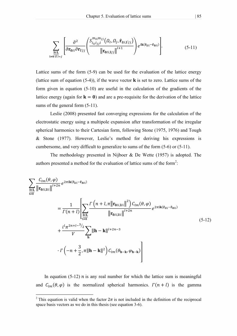
Chapter 5. Evaluation of lattice sums | 85
(5-11)
Lattice sums of the form (5-9) can be used for the evaluation of the lattice energy
(lattice sum of equation (5-4)), if the wave vector is set to zero. Lattice sums of the
form given in equation (5-10) are useful in the calculation of the gradients of the
lattice energy (again for ) and are a pre-requisite for the derivation of the lattice
sums of the general form (5-11).
Leslie (2008) presented fast converging expressions for the calculation of the
electrostatic energy using a multipole expansion after transformation of the irregular
spherical harmonics to their Cartesian form, following Stone (1975, 1976) and Tough
& Stone (1977). However, Leslie‘s method for deriving his expressions is
cumbersome, and very difficult to generalize to sums of the form (5-6) or (5-11).
The methodology presented in Nijboer & De Wette (1957) is adopted. The
authors presented a method for the evaluation of lattice sums of the form2:
(5-12)
In equation (5-12) is any real number for which the lattice sum is meaningful
and is the normalized spherical harmonics. is the gamma
2 This equation is valid when the factor is not included in the definition of the reciprocal
space basis vectors as we do in this thesis (see equation 3-6).

Chapter 5. Evaluation of lattice sums | 86
function, while is the upper incomplete gamma function, which is related
to the lower incomplete gamma function, , and the gamma function by
(Abramowitz & Stegun, 1972):
. (5-13)
is a reciprocal lattice vector, while is a reciprocal space vector. The first
summation on the right hand side of equation (5-12) is known as a direct space sum or
real space sum, while we refer to the second as a reciprocal space sum.
The applicability of equation (5-12) is limited to the case of the sum of a property
of periodic images, i.e. . Furthermore in equation (5-12) there is no Ewald
convergence parameter (Frenkel & Smit, 2002), whose existence is very convenient
for optimisation of the relative rate of convergence between the reciprocal and the
direct space sums. As a result we propose a modified version of equation (5-12) that
can be used for an arbitrary pair of atoms and we also introduce the Ewald
convergence parameter . To do so, we follow the procedure described in Nijboer &
De Wette, (1957). A similar generalization of Nijboer & De Wette‘s method has also
been published by Grant (1965:a,1965:b). His result is apparently different and further
discussion on this issue will follow after the presentation of the method. Here we do
not present in detail all the derivation but only the key intermediate results.
The proof is developed by introducing an auxiliary function, F , that
transforms the sum of interest in the following way
(5-14)
The second sum on the right hand of equation (5-14) is the reciprocal sum, because it
can only be calculated (after Fourier transformation) in the reciprocal space. We
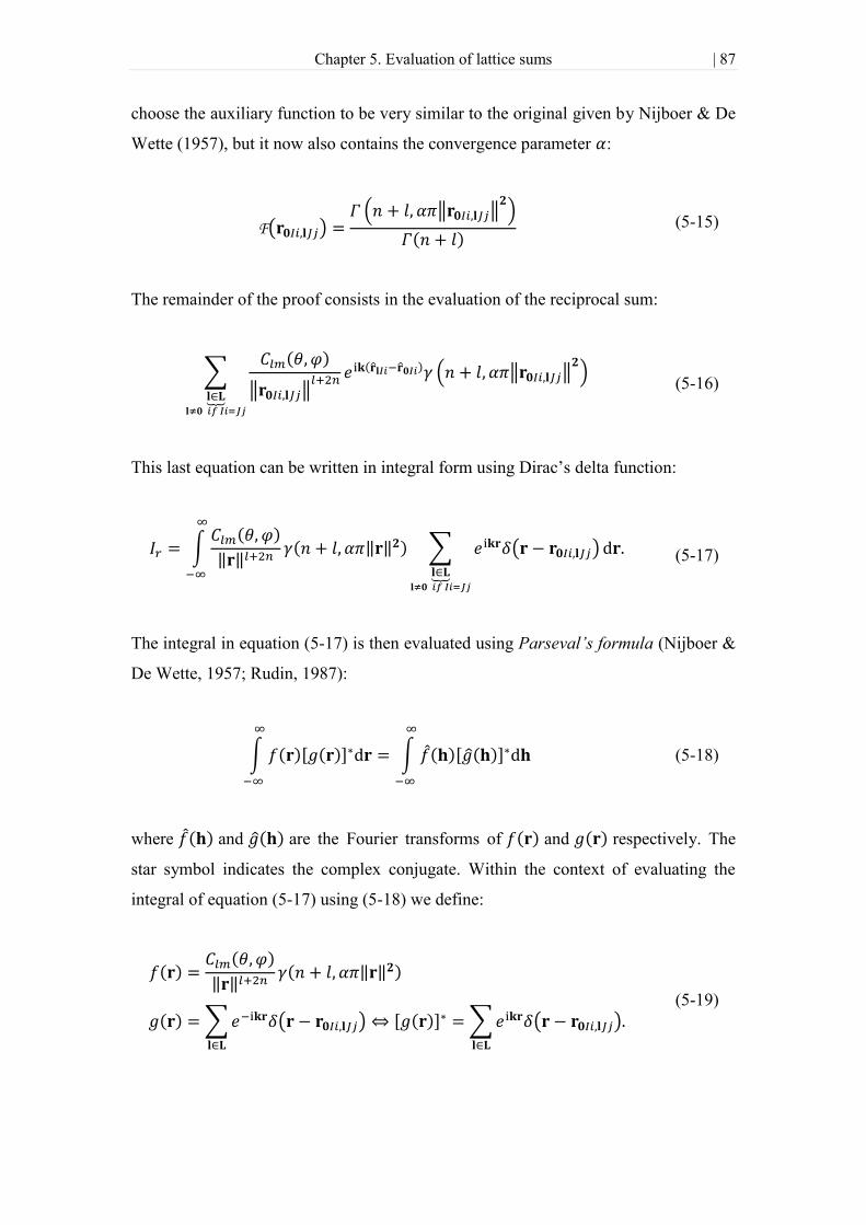
Chapter 5. Evaluation of lattice sums | 87
choose the auxiliary function to be very similar to the original given by Nijboer & De
Wette (1957), but it now also contains the convergence parameter :
(5-15)
The remainder of the proof consists in the evaluation of the reciprocal sum:
(5-16)
This last equation can be written in integral form using Dirac‘s delta function:
(5-17)
The integral in equation (5-17) is then evaluated using Parseval’s formula (Nijboer &
De Wette, 1957; Rudin, 1987):
(5-18)
where and are the Fourier transforms of and respectively. The
star symbol indicates the complex conjugate. Within the context of evaluating the
integral of equation (5-17) using (5-18) we define:
(5-19)

Chapter 5. Evaluation of lattice sums | 88
Following Nijboer & De Wette (1957) we can prove that the Fourier transform, ,
of as defined by equation (5-19) is:
(5-20)
A crucial step in deriving equation (5-20) is the evaluation of the integral:
(5-21)
where α is the Bessel function (Abramowitz & Stegun, 1972). The equality can be
proved using the general expression (Watson, 1944):
(5-22)
The evaluation of , the Fourier transform of , described in (5-19), is also
carried out along the lines described by Nijboer & De Wette (1957):
(5-23)
Finally by substitution of equations (5-19), (5-20) and (5-23) into equation (5-18), we
can obtain an expression for the integral, , of equation (5-17):
(5-24)
where is the Kronecker delta and is the self-correction term given by:

Chapter 5. Evaluation of lattice sums | 89
(5-25)
For our purpose (i.e. the evaluation of summation (5-4)), the suitable sum is that for
which
, which is summarized as:
(5-26)
To obtain the last result we have used the identity:
Finally, it is trivial to derive the necessary expression for sum (5-4) if we substitute
equation (4-36) into expression (5-26):
Chapter 5. Evaluation of lattice sums | 90
(5-27)
In this last expression the self correction term is now given by:
(5-28)
The evaluation of limit (5-28) for the case
, which is the one we are interested
in, is straightforward thanks to the definition of the lower incomplete gamma
function,
:
(5-29)
5.3.1. Calculation of the lattice energy of molecular crystals
In the case of molecular crystals modeled according to the approach described in
Chapter 4, it is necessary to exclude from the lattice sum in equation (5-27) the term
arising from the interactions of atoms that belong to the same molecule. This is
necessary in order to avoid the double counting of the electrostatic interactions
between these atoms, which are already included in the intra-molecular contribution
Chapter 5. Evaluation of lattice sums | 91
computed using ab-initio calculations. This is done by means of a molecular
correction term (Karamertzanis, 2004) that is added to the right side of equation
(5-27). Note also that the terms excluded from the lattice sum of equation (5-27) are
not the same as those excluded from the required lattice sum (equation 5-9).
The appropriate functional form of the molecular correction term is obtained
by subtracting the term to be excluded from both sides of equation (5-27). On the left
hand side, this implies removing components of the summation corresponding to the
interactions of any two atoms in the same molecule in reference unit cell (i.e., for l =
0,. I=J but i not necessarily equal to j). Then we have:
(5-30)
Equation (5-30) provides a transformation of the general lattice sum (5-9) into
two rapidly converging series. This result can be used to evaluate the electrostatic
contribution to the lattice energy (equation (5-4)). Equation (5-30) is valid for any
wave vector , and therefore for , which if substituted into (5-30) leads directly to
lattice sum (5-4). The calculation of the lattice energy by substitution of equation
(5-27) or equation (5-30) into (5-3) gives identical results to those obtained when
using the formalism presented in Leslie (2008). One difference between the two
approaches is that the general form of the lattice sum (5-9) which we use for the

Chapter 5. Evaluation of lattice sums | 92
evaluation of the lattice energy represents a wider class of sums than the sums for
which Leslie (2008) provides a fast converging expression.
It might seem surprising that in the reciprocal sum of expressions (5-27) and
(5-30) the reciprocal space vector appears instead of , which is often
found in similar expressions (Aung & Strauss, 1973; Fuchizaki, 1994, 2010; Nijboer
& De Wette, 1957; Grant, 1965:a). This is a consequence of our choice of the
functions and (equation 5-19) for the application of Parseval‘s formula.
This choice was made for convenience and it is trivial to prove that if the opposite
definition was chosen then would appear with opposite sign. In addition it is easy to
prove that for the lattice sums that are of interest in Aung & Strauss (1973), and
Fuchizaki (1994, 2010) the sign of the wave vector does not affect the value of the
reciprocal sum. Furthermore these particular sums are not of interest here so they are
not discussed further. On the other hand in the lattice sums (5-27) and (5-30) as well
as the very closely related lattice sums presented in Nijboer & De Wette (1957) and in
Grant (1965:a), the sign of in principle affects the value of the reciprocal sum.
These authors seem to have ignored, without stating a reason, the fact that in equation
(5-18) the complex conjugate of the Fourier transform of (equation (5-19)) is
required. Finally the wave vector in the reciprocal sum of the Ewald expression for
the field of a lattice of dipoles presented in Born & Huang (1954) appears with a
positive sign.
A visual demonstration of the way in which the Ewald summation technique
operates is presented in this section based on an analysis of the individual
contributions to the electrostatic energy of the monoclinic form (Chaplot et al., 1984)
of tetracyanoethylene (see Figure 5-1, p.93). The different contributions to the
electrostatic energy of the predicted structure, from charge-charge to charge-
quadrupole, are plotted against the value of the Ewald convergence parameter ― ‖ of
equation (5-30). Furthermore the various components of the Ewald method, namely
the direct space, reciprocal space, molecular correction and self correction
contributions, are also plotted as function of the parameter . Details of the
computational model used and the structure are presented in section 6.4.2, where an
in-depth study of tetracyanoethylene is undertaken.
The charge-charge contribution is shown in Figure 5-2, the charge-dipole
contribution is shown in Figure 5-3, the charge-quadrupole contribution is shown in

Chapter 5. Evaluation of lattice sums | 93
(a) (b)
Figure 5-1 (a) The chemical diagram of tetracyanoethylene and (b) the experimental unit
cell of the monoclinic form at 298K.
Figure 5-4 and the dipole-dipole contribution is shown in Figure 5-5. The cut-off of
the direct space sum is 17Å, while reciprocal cells up to the 6th
are considered in the
reciprocal sum. These parameters are sufficiently large to ensure that the sums are
converged. It is apparent that for every contribution, although the different
components of the sum vary significantly with the value of ― ‖, the total contribution
is unaffected by this choice. This is intuitively understood as the cancellation of the
error induced in the lattice sum by the auxiliary function (5-15), by the other
components (reciprocal space sum, molecular and self correction). This is a validation
of equations (5-27) and (5-30). Such a validation can also be achieved by following
the approach of Fuchizaki‘s (2010), i.e., by proving that the gradient of the right part
of equation (5-30) with respect to vanishes. If the gradient is zero the total
contribution is a constant function of , which implies that the modification incurred
in the lattice sum by the presence of the auxiliary function (5-15) in the real space
sum is fully compensated by the other terms, namely the reciprocal space sum, the
molecular correction, and the self correction (equation 5-14).
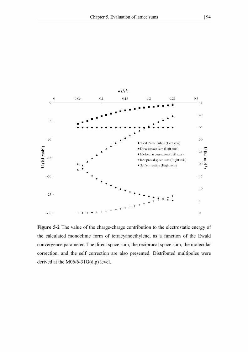
Chapter 5. Evaluation of lattice sums | 94
Figure 5-2 The value of the charge-charge contribution to the electrostatic energy of
the calculated monoclinic form of tetracyanoethylene, as a function of the Ewald
convergence parameter. The direct space sum, the reciprocal space sum, the molecular
correction, and the self correction are also presented. Distributed multipoles were
derived at the M06/6-31G(d,p) level.

Chapter 5. Evaluation of lattice sums | 95
Figure 5-3 The value of the charge-dipole contribution to the electrostatic energy of
the calculated monoclinic form of tetracyanoethylene, as function of the Ewald
convergence parameter. The direct space sum, the reciprocal space sum, and the
molecular correction are also presented. Distributed multipoles were derived at the
M06/6-31G(d,p) level.

Chapter 5. Evaluation of lattice sums | 96
Figure 5-4 The value of the charge-quadrupole contribution to the electrostatic energy
of the calculated monoclinic form of tetracyanoethylene, as function of the Ewald
convergence parameter. The direct space sum, the reciprocal space sum, and the
molecular correction are also presented. Distributed multipoles were derived at the
M06/6-31G(d,p) level.

Chapter 5. Evaluation of lattice sums | 97
Figure 5-5 The value of the dipole-dipole contribution to the electrostatic energy of
the calculated monoclinic form of tetracyanoethylene, as function of the Ewald
convergence parameter. The direct space sum, the reciprocal space sum, and the
molecular correction are also presented. Distributed multipoles were derived at the
M06/6-31G(d,p) level.

Chapter 5. Evaluation of lattice sums | 98
5.3.2. Efficient summation scheme for the dynamical matrix
In this section a method for the efficient evaluation of the lattice sums of
equations (5-10) and (5-11) is derived. Lattice sum (5-11) is necessary for the
efficient evaluation of the electrostatic contribution to the dynamical matrix
(essentially the sum of equation (5-6)). On the other hand, lattice sum (5-10) is a
necessary intermediate step, which can find use in the evaluation of the gradient of the
lattice energy, but it is not used for calculations presented in this thesis. The starting
point is the equation derived for the calculation of the lattice energy (equation 5-27).
Following Signorini et al. (1991), we differentiate equation (5-27) with respect to ,
and we subsequently subtract equation (5-27) multiplied by .
The following result is obtained:
(5-31)
The self correction term
is equal to:
(5-32)

Chapter 5. Evaluation of lattice sums | 99
The derivative involved in expression (5-32) is obtained using the definition of the
self correction of the lattice energy (equation 5-28), carrying out the differentiation
before the calculation of the limit. If the opposite order is followed, i.e.,
differentiation of equation (5-29), an invalid result is obtained in which the value of
the lattice sum depends on the chosen value of the parameter , contrary to
expectations. The value of the self correction term
in terms of
the local axis system of molecule defined by the unit vectors , and and the
corresponding vectors rigidly fixed on molecule : , and is summarized in
Table 5-1. One very interesting feature of the tabulated values is that none of them
depends on the wave vector .
Following the same procedure we obtain the following expression for the lattice
sum of second derivatives:
0
0
Table 5-1 The self correction term for the different components of the various
contributions to the electrostatic energy gradient (equation 5-31).

Chapter 5. Evaluation of lattice sums | 100
(5-33)
where the self correction term
is
(5-34)
The values of the self correction term
are presented in detail in
Appendix B.
In the case of molecular crystals where the dynamical matrix calculation requires
the evaluation of a lattice sum of the form (5-11), it is necessary to include a
―molecular correction term‖ in equation (5-33), in a way that is equivalent to the
molecular correction term for the lattice energy that was described in section 5.3.1.
This is done as described in section 5.3.1, and the expression that is obtained is:

Chapter 5. Evaluation of lattice sums | 101
(5-35)
The validity of equation (5-35) is assessed graphically in a similar way as
equation (5-30) in section 5.3.1. Figure 5-7 shows the value of one component of the
charge/dipole contribution to the element of matrix associated with the interaction
between the third and second atom (and its periodic images) of the first molecule in
the unit cell (see Figure 5-6,a), as function of the convergence parameter . A three-
dimensional plot is needed because matrix mplex. Figure 5-8 is a projection of
matrix onto the complex plane. The wave vector was chosen arbitrarily to be
(a) (b)
Figure 5-6 (a) The element of the dynamical matrix is related the interaction
of the red atom ( ) with the atom and its periodic images (green). (b)
The element of the dynamical matrix is related to the self-interaction of the
green atoms ( )
Chapter 5. Evaluation of lattice sums | 102
Figure 5-9 is obtained in a similar manner to Figure 5-7 but is used to
display a component of the charge quadrupole contribution for the element of matrix
related to the self-interaction of the first atom of the first molecule, and its periodic
images (see Figure 5-6,b) and for the same wave vector. Since the chosen contribution
happens to be real, Figure 5-10 shows a projection on the plane defined by the real
part of the dynamical matrix element and the parameter . All these plots show a
behavior independent of the chosen value of parameter , a result which is identical to
that obtained for the lattice energy (see figures in section 5.3.1)

Chapter 5. Evaluation of lattice sums | 103
Figure 5-7 The value of the component (0,1s) of the charge-dipole contribution to the
element of matrix (defined in equation 4-22, page 63), for
as function of the Ewald convergence parameter α. The calculation is performed for
the predicted structure that corresponds to the monoclinic form of tetracyanoethylene
(see section 6.4.2). The quantum mechanical calculations were performed at the
M06/6-31G(d,p) level. The direct space sum and the reciprocal space sum are also
shown.

Chapter 5. Evaluation of lattice sums | 104
Figure 5-8 A projection onto the complex plane of the dynamical matrix element
shown in Figure 5-7. The correction term and the direct and reciprocal space sums are
also shown.

Chapter 5. Evaluation of lattice sums | 105
Figure 5-9 The value of the component (0,2c) of the charge-quadruple contribution to
the element of matrix (defined in equation (4-22), page 63), for
as a function of the Ewald convergence parameter α. The calculation is
performed for the predicted structure that corresponds to the monoclinic form of
tetracyanoethylene (see section 6.4.2). The quantum mechanical calculations were
performed at the M06/6-31G(d,p) level. The direct space sum and the reciprocal space
sum are also shown.

Chapter 5. Evaluation of lattice sums | 106
Figure 5-10 A projection onto the plane defined by the real part of the dynamical
matrix element shown in Figure 5-9, and the α parameter. The correction term and
the direct and reciprocal space sums are also shown.

Chapter 5. Evaluation of lattice sums | 107
5.4. The Γ-point in the reciprocal space sum
In equations (5-27), (5-30) the contribution of the -point, , to the
reciprocal lattice sum is undefined if the wave vector for and therefore it
is omitted. The same behaviour is observed in the reciprocal sum of equations (5-33),
(5-35) for . Therefore the lattice sums of interest for the calculation of the lattice
energy and the dynamical matrix take the form:
(5-36)
and

Chapter 5. Evaluation of lattice sums | 108
(5-37)
respectively. The fact that the point is omitted in reciprocal sum
(5-36) clearly does not affect interactions for which . The same is true in
equation (5-37) for interactions for which .
The omitted terms do not have a contribution to the lattice sums of
centrosymmetic unit cells crystals, while for non-centrosymmetric unit cells these
terms have a finite contribution. The way the contribution of the Γ-point to reciprocal
lattice sums (5-36) and (5-37) can be calculated has been discussed by many authors
(Born & Huang, 1954; de Leeuw et al., 1980; Deem et al., 1990; Nymand & Linse,
2000; Smith, 1981; van Eijk & Kroon 1997; Minicozzi & Stroot, 1971) for several
specific cases. This term is known to have an effect similar to that of an external field
(Born & Huang, 1954) and it is associated with non-zero charge at the surface of polar
crystals. It is commonly referred to as the surface correction term. In contrast to any
other term in the lattice sums, this value of this term depends on the crystal‘s shape.
Its dependence on the shape of the crystal has led to some discussions in the literature
questioning whether it should be included or not (Pillardy et al., 2000; van Eijk &
Kroon, 1997, 2000; Wedemeyer et al., 2000), especially in the course of a crystal
structure prediction study based on lattice energy calculations. The main argument

Chapter 5. Evaluation of lattice sums | 109
against the use of the term is that ―material‖ external to the crystal needs to
accumulate at the surface in order to cancel the surface charge which is responsible
for this term (van Eijk & Kroon, 1997, 2000). This is known as the tin foil boundary
condition and is a reasonable assumption when the crystal is grown from a solvent
with a high dielectric constant. Furthermore, in the course of a crystal structure
prediction study, the crystal shape is not known and therefore it is challenging to
include this term in a meaningful way. On the other hand it is argued that there are
some cases where the conditions under which the surface correction term is negligible
are not met (Pillardy et al., 2000; Wedemeyer et al., 2000). Therefore, surface
correction term cannot be regarded as negligible in all cases, and its importance
should in principle be assessed in each new study.
With regards to lattice dynamics calculations, there is evidence suggesting that
this term does not significantly affect the result (Aung & Strauss, 1973; van Eijk,
2001). Finally the compatibility of the surface correction term with the Born & von
Kàrmàn cyclic boundary condition that is adopted in lattice dynamics calculations is
not clear. Here, we omit it following van Eijk & Kroon (1997, 2000).
Chapter 6. Results | 110
6. Results
In this chapter the extension of a crystal structure prediction methodology
through the integration of a methodology for the calculation of the free energy based
on the harmonic approximation is investigated. As a first test of the approach, the fcc
crystal of argon (Ar) is studied within the harmonic approximation. The Ar crystal is
modeled as an fcc Lennard-Jones crystal. Then the methodology that we adopt for
crystal structure prediction is briefly described and is subsequently applied to
imidazole and tetracyanoethylene. The free energies, from 0 K to the melting point, of
the low-lying lattice energy minima of imidazole and tetracyanoethylene are
evaluated as described in chapters 3,4 and 5. A small investigation of the effect of the
chosen model on the calculations is also presented. Finally the free energy, from 0 K
to 80 K, of the ambient pressure crystal of Ar is calculated using a quasi-harmonic
free energy minimisation algorithm. This allows changes in the structure of Ar as a
function of temperature to be determined.
6.1. The Lennard-Jones solid; Dispersion
curves and density of states
A solid of Lennard-Jones spheres (Choi et al., 1993; Kaplan, 2006; Lennard-
Jones, 1937) is a useful model system that allows the initial validation of the
harmonic approximation method. In such a system, particles are held together because
they interact isotropically via the Lennard-Jones potential (see section 4.3). The
Lennard-Jones model system offers a good description of real solids that interact
primarily via repulsion and dispersion interactions such as the rare gas solids, such as
argon, krypton, xenon. In this work, the Lennard-Jones potential is used to study
argon (Ar), whose crystalline form has been extensively studied experimentally at

Chapter 6. Results | 111
temperatures up to its melting point (84 K, Dobbs & Jones, 1957) and for which
different types of measured data are available. Argon is known to crystallize in a face
centered cubic (fcc) lattice at ambient pressure (Born & Huang, 1954).
Many different sets of Lennard-Jones parameters for Ar can be found in the
literature (Diemand et al., 2013; Freeman & Doll, 1985; Goharshadi et al., 2007;
Özgen et al., 1996; Kittel 2005, Laasonen et al., 2000; Rahman, 1964; Salonen et al.,
2007; Singer & Smith, 1987; White 1999). Here we are not interested in the optimal
model for the description of argon but in an investigation of the capabilities of method
of harmonic approximation. Therefore no assessment of the reliability of the various
sets was attempted. We use values proposed by Rahman (1964) in the study of the
dynamics of liquid argon, specifically and Å. Most of the
various other parameters sets differ slightly from these values, with the largest
differences observed for , which in the vast majority of cases varies by only
. Another popular choice for the parameter is only higher.
The most stable structure is known qualitatively (fcc), and the lattice constant
describing the unit cell has been measured by Barrett & Meyer (1964) as 5.311 Å at
4.2 K and by Peterson et al. (1966) as 5.30017 Å at 4.25 K. Here, the lattice constant
is computed by determining the global minimum of the lattice energy function. For
comparison with the experimental dispersion curves, it is necessary to use the
primitive unit cell, which is rhombohedral (Hawkins et al., 2008). The lattice energy
and its derivatives are calculated in a pairwise additive manner as described in section
4.2, without any consideration of the efficiency of convergence of the lattice sum, or
any correction for the potential tail region. In order to limit the negative effects of
such an approach, a large radial cut-off distance equal to is used; in the case of
Ar, this is equal to the very large value of Å. Lattice energy minimization is
performed with respect to the lattice lengths and lattice angles, using the BFGS
method, which does not require a calculation of the Hessian. This confirms that a fcc
primitive cell (α,β,γ=60ο and a=b=c) is reproduced by the chosen potential. The
minimum energy lattice constant of Ar is 5.25 Å. As soon as the lattice energy
minimum is obtained, harmonic properties such as the phonon frequencies and the
density of vibrational states can be calculated.
The dispersion curves of Ar along three high symmetry directions, ,
and , are shown in Figure 6-1. Because the primitive unit cell of the

Chapter 6. Results | 112
Figure 6-1 Dispersion curves of Argon when the wave vectors vary along three
directions , , and , as a function of the reduced wave vector
coordinate . The dots are the calculated points, while the triangles are experimental
data (Fujii et al., 1974).
fcc crystal contains only one atom, there are three modes of vibration described by
three branches on the dispersion curves. Along directions and two
modes coincide as a result of the high symmetry of the crystal. Experimental points
(Fujii et al., 1974) for every mode and along all directions compare very well with the
calculated values.
The density of vibrational states, shown in Figure 6-2, is generated as described
in section 3.6, based on one million randomly sampled wave vectors and is
normalized to unity. It is found to be in good qualitative agreement (within a
multiplicative constant) with the density of states calculated using the method of Gilat
& Raubenheimer (1966), as reported in Fujii et al. (1974). A quadratic function is
also fitted to the low frequency region of the density of states ( THz ). The fit
was obtained in MS Excel, and it shows that in this region, the density of states can
indeed be approximated by a quadratic function verifying the validity of the Debye
approximation (see section 3.7).

Chapter 6. Results | 113
(a)
(b)
Figure 6-2 (a) Normalized density of vibrational states as a function of frequency;
(b) a close-up of the normalized density of states in the low frequency region. A
quadratic trend curve is also fitted to the low frequency region and shown in red.

Chapter 6. Results | 114
6.2. Crystal structure prediction methodology
It is common practice to perform crystal structure prediction based on
optimization algorithms in which the lattice energy function is used as an objective
function (Day, 2011; Price, 2008). A distinctive characteristic of crystal structure
prediction as an optimization problem is that it is not sufficient to look for the global
minimum, but that all low-energy minima are sought. This is because one is interested
in metastable polymorphs that are higher in energy than the most stable polymorph,
but also because this helps to overcome the limitations of existing techniques, in
which model uncertainty may lead to inaccuracies in the relative energies of different
structures.
6.2.1. Overview of the approach
From a practical perspective, it is known (Lommerse et al., 2000; Motherwell et
al., 2002; Day et al., 2005,2009; Bardwell et al., 2011) that the reliable modeling of
the organic solid state requires highly accurate and hence computationally-demanding
models. As a consequence, it is necessary to adopt a hierarchical methodology to
crystal structure prediction in order to achieve reasonable efficiency. Our group has
been performing crystal structure prediction studies over the past years using a
multistage methodology, tackling different problems at different stages.
1) Stage 1. A conformational analysis is performed based on a survey of the
Cambridge Structural Database (CSD), and isolated molecule quantum
mechanical calculations. The purpose is to identify the set of intra-
molecular degrees of freedom that must to be treated as flexible during
stage 2, as well as their range of variation. Furthermore, an appropriate
model is chosen for the inter-atomic interactions, as specified by a level of
theory and a basis set for isolated molecule quantum mechanical
calculations, and a semi-empirical model for the repulsion and dispersion
interactions with an associated set for parameters.
2) Stage 2. A global search is carried out with the aim to identify all low
energy minima of the lattice energy hyper-surface. The number of minima
identified is of the order of millions and a simplified model is adopted to

Chapter 6. Results | 115
achieve this. This stage is performed using the CrystalPredictor algorithm
(Karamertzanis & Pantelides, 2005, 2007)
3) Stage 3. The most promising minima (i.e., with the lowest lattice energy)
identified in the previous stage are further minimized using a much more
accurate, and hence computationally-demanding model:
a. In the case of rigid molecules, accuracy is increased by using a
more detailed model for the electrostatic interactions, based on a
distributed multipole expansion. The DMACRYS software is used
for this purpose (Price et al., 2010).
b. In the case of flexible molecules higher accuracy is achieved in one
or more ways: by using a more detailed model for the electrostatic
interactions, based on a distributed multipole expansion, by
allowing additional molecular flexibility, and by calculating the
intra-molecular energy with a higher quantum mechanical level of
accuracy. In this case the CrystalOptimizer algorithm (Kazantsev et
al., 2010, 2011:a) is used.
4) Stage 4: In the final analysis stage, additional criteria can be used to
identify the most likely polymorphs from the ranking generating. This may
include more accurate calculations on selected structures or the evaluation
of additional information. In this work, this stage is extended to include a
re-ranking based on the results of free energy calculations under the
harmonic approximation.
6.2.2. Comparison of crystal structures
The program COMPACK (Chisholm & Motherwell, 2005) is used for assessing the
similarity of any two crystals. The default settings of 15 molecules in the coordination
sphere and 20% for the angle and distance tolerance are used. In this way the
geometry of a cluster of 15 molecules in one structure is compared with that of the
equivalent cluster in the other structure. The quantification of the difference between
the two structures is done by a root mean squared deviation of the atomic positions,
rms15. The subscript 15 implies that the coordination sphere consists of 15 molecules.
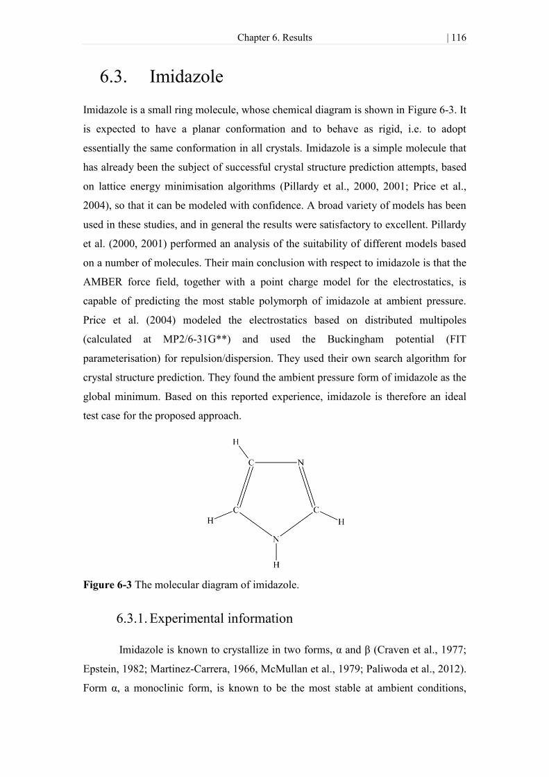
Chapter 6. Results | 116
Figure 6-3 The molecular diagram of imidazole.
6.3. Imidazole
Imidazole is a small ring molecule, whose chemical diagram is shown in Figure 6-3. It
is expected to have a planar conformation and to behave as rigid, i.e. to adopt
essentially the same conformation in all crystals. Imidazole is a simple molecule that
has already been the subject of successful crystal structure prediction attempts, based
on lattice energy minimisation algorithms (Pillardy et al., 2000, 2001; Price et al.,
2004), so that it can be modeled with confidence. A broad variety of models has been
used in these studies, and in general the results were satisfactory to excellent. Pillardy
et al. (2000, 2001) performed an analysis of the suitability of different models based
on a number of molecules. Their main conclusion with respect to imidazole is that the
AMBER force field, together with a point charge model for the electrostatics, is
capable of predicting the most stable polymorph of imidazole at ambient pressure.
Price et al. (2004) modeled the electrostatics based on distributed multipoles
(calculated at MP2/6-31G**) and used the Buckingham potential (FIT
parameterisation) for repulsion/dispersion. They used their own search algorithm for
crystal structure prediction. They found the ambient pressure form of imidazole as the
global minimum. Based on this reported experience, imidazole is therefore an ideal
test case for the proposed approach.
6.3.1. Experimental information
Imidazole is known to crystallize in two forms, α and β (Craven et al., 1977;
Epstein, 1982; Martinez-Carrera, 1966, McMullan et al., 1979; Paliwoda et al., 2012).
Form α, a monoclinic form, is known to be the most stable at ambient conditions,

Chapter 6. Results | 117
while the cubic β form is stable at high pressures (greater than 0.5 GPa). The major
characteristics of the two unit cells are summarized in Table 6-1. A visualisation of
the unit cell of the two polymorphs of imidazole is found in Figure 6-4.
The normal melting point of imidazole is 364 K; no other form other than α
has been observed experimentally from 103 K, the lowest temperature at which
experiments have been performed, to the melting point (Paliwoda, 2012). As a
consequence we do not expect a polymorphic phase transition to occur in our study.
Finally to the best of our knowledge, there are no available dynamical information,
i.e., frequencies of vibration.
6.3.2. Crystal structure prediction
The crystal structure prediction methodology described in section 6.2 is
applied to imidazole. The molecule is treated as rigid during the search stage and
(a) (b)
Figure 6-4 Visualisation of the experimental unit cells of the two forms of imidazole
a) the unit cell of the α-form at 103 K and ambient pressure (McMullan et al., 1979) ;
b) the unit cell of the β-form at 298K and 0.8GPa (Paliwoda et al., 2012).
Form Space
group Z' Z a (Å) b (Å) c (Å) β (
o) π ( g cm
-3)
α (103K) P21/c 1 4 7.57 5.37 9.79 119.08 1.300
α (293K) P21/c 1 4 7.73 5.45 9.78 117.28 1.235
β (298K/0.8GPa) Aba2 1 8 13.91 8.60 5.34 90.00 1.416
Table 6-1 Basic characteristics of the unit cell of the two resolved forms of
imidazole. Lattice angles α and γ are equal to 90o for all forms at all temperatures
because of symmetry constraints.

Chapter 6. Results | 118
therefore stage 1 consists only of the determination of the conformation of imidazole,
namely the gas phase conformation (the unconstrained global minimum) obtained at
the MP2/6-31G(d,p) level. The repulsion and dispersion interactions are calculated
using the Buckingham potential with the FIT parameterization described in section
4.3. During stage 2 atomic point charges are used to model the electrostatic
interactions. The point charges are derived using the ChelpG method (Breneman &
Wiberg, 1990) from the ab-initio derived electrostatic potential calculated at the
MP2/6-31G(d,p) level of theory for the gas phase conformation.
The search stage is performed with the rigid version of the CrystalPredictor
algorithm (Karamertzanis & Pantelides, 2005). Half a million crystals are generated in
59 commonly encountered space groups: , , , , , ,
, , , , , , , , , , , , ,
, , , , , , , , , ,
, , , , , , , , , , , ,
, , , , , , , , , , , , ,
, , and . It is assumed that there is only one molecule in the
asymmetric unit. The global search results in the identification of 811 structures
within 10 kJ mol-1
of the global minimum and 3263 structures within 15 kJ mol-1
of
the global minimum. The global search identifies the β-form of imidazole as the
global minimum with an rms15 equal to 0.272Å, while the α-form corresponds to the
6th
lowest energy minimum with a match of the experimental structure quantified by
an rms15=0.200Å.
The 200 unique lowest energy structures generated by CrystalPredictor are
minimised in Stage 3 using the DMACRYS local lattice energy minimisation program
(Price et al., 2010), in which a more accurate representation of the electrostatic
interactions is used. The gas-phase conformation and energy are re-calculated at the
M06/6-31G(d,p) level. Distributed multipoles up to hexadecapole are determined
based on the wave function of the resulting gas phase conformation. In general several
of the structures obtained at the global search stage may lead to the same minimum
during the structure refinement in stage 3. In this case, our final landscape consists of
149 unique structures. Moreover, during 19 of the 200 minimizations, a symmetry
reduction was performed because the final structure was found to be a saddle point,
giving 19 =2 structures. The final lattice energy landscape is shown in Figure 6-5.

Chapter 6. Results | 119
Figure 6-5 Final lattice energy landscape of imidazole. Red dot and diamond
represent the experimentally known α and β forms. Quantum mechanical calculations
were performed at M06/6-31G(d,p) level.
The α-form is correctly predicted as the most stable structure with rms15=0.133Å,
while the β-form, which is unstable at ambient pressure, is found to be 16th
lowest-
energy structure. The rms15 for the β-form is 0.421Å. These differences can be
visualized on Figure 6-6 where the experimental and predicted structures are overlaid.
Figure 6-6 Overlay between the predicted (green) and experimental (coloured by
element) forms of imidazole. a) the α-form, with rms15=0.133Å, b) the β-form, with
rms15=0.425Å. Quantum mechanical calculations were performed at the Μ06/6-
31G(d,p) level.
.

Chapter 6. Results | 120
It should be pointed out that the β-form is predicted as the densest structure compared
to the other predicted structures, in line with the experimental evidence that it is
stabilized via pressurisation.
6.3.3. Temperature effects in crystal structure prediction
The free energy landscape is constructed from 0 K to 350 K, very close to the
melting point. Integration of the free energy expression (equation 3-33) is carried out
using the Gauss-Legendre quadrature (see section 3.7) over a 64-node grid in the
reciprocal unit cell. The Helmholtz free energy landscapes at 0 K, 100 K, 200 K, 300
K and 350 K are shown in Figure 6-7, Figure 6-8 and Figure 6-9. The dots in Figure
6-7 to Figure 6-9 are coloured based on the change in rank of the corresponding
structure from the lattice energy landscape to that including the vibrational
contributions to the free energy, i.e. based on the value of the quantity R R ,
where R is the rank of the structure in the free energy landscape at temperature
and R is the rank in the lattice energy landscape.
Dynamical calculations reveal that 18 structures are unstable, corresponding
approximately to 12% of the structures generated in stage 3. This leads to changes in
the rank of remaining structures, especially the highest energy ones.
Temperature is found to affect mainly the high free energy structures, while the
lowest ranked structures practically remain unaffected. Somewhat unexpectedly at
first, the structures that are in the high free energy region appear to achieve an
improved rank (they are coloured in blue tones) even at low temperatures. This can in
fact be attributed to the elimination of some of the structures with a lower lattice
energy as unstable. The stable α-form remains the most stable structure for the whole
range of temperatures from 0 K to the melting point. The rank of the unstable β-form
deteriorates with increasing temperature.
In order to investigate the effect of the choice of computational model, these
calculations are repeated for at the HF/6-31G(d,p) level of theory. The free energy
and rank as function of temperature for the two forms, for the HF and M06 level, are
summarized in Table 6-2. A similar result is obtained with both models, although
some re-ordering of the low energy minima is observed for HF at higher temperatures.
The structure that is the global minimum for 300 K and 350 K in the HF/6-
31G(d,p) landscapes is very closely related to the structure that corresponds to the α-

Chapter 6. Results | 121
(K)
M06/6-31G(d,p) HF/6-31G(d,p)
α-form β-form α-form β-form A
(kJ mol-1
) Rank
A
(kJ mol-1
) Rank
A
(kJ mol-1
) Rank
A
(kJ mol-1
) Rank
0 -68.69 1 -63.95 16 -78.08 1 -69.99 31
50 -69.03 1 -64.23 16 -78.37 1 -70.22 32
100 -70.61 1 -65.68 17 -79.79 1 -71.52 32
200 -76.76 1 -71.55 19 -85.50 1 -76.96 38
300 -85.86 1 -80.38 21 -94.00 2 -85.21 39
350 -91.42 1 -85.80 21 -99.17 2 -91.02 41
-73.83 1 -69.06 16 -83.80 1 -75.56 30
Table 6-2 Summary of the lattice energy, rank and the Helmholtz free energy of
the α and β forms of imidazole, as function of temperature.
form. Its deviation (rms15) from the experimental structure is 0.442Å; from the
predicted structure that corresponds to the experimental form, it is 0.234Å only. The
rms15 of the β-form for the HF calculation is 0.420Å. The complete free energy
landscapes for the HF calculations are not presented.

Chapter 6. Results | 122
(a)
(b)
Figure 6-7 The Helmholtz free energy landscape of imidazole at (a) 0 K ; (b) 100 K.
All necessary quantum mechanical (charge density and geometry) calculations were
performed at M06/6-31G(d,p) level. The colour scale describes the difference in the
rank of each structure before and after the vibrational contributions are included.
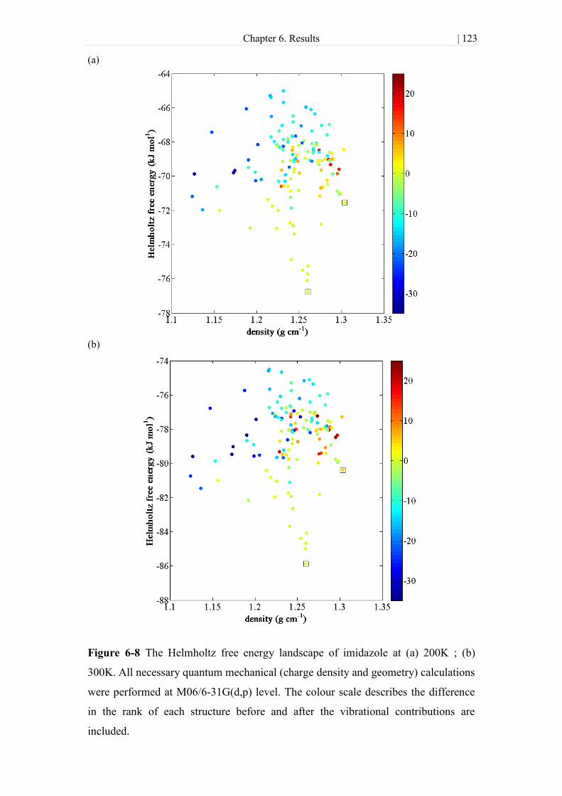
Chapter 6. Results | 123
(a)
(b)
Figure 6-8 The Helmholtz free energy landscape of imidazole at (a) 200K ; (b)
300K. All necessary quantum mechanical (charge density and geometry) calculations
were performed at M06/6-31G(d,p) level. The colour scale describes the difference
in the rank of each structure before and after the vibrational contributions are
included.

Chapter 6. Results | 124
Figure 6-9 The Helmholtz free energy landscape of imidazole at 350K. All
necessary quantum mechanical (charge density and geometry) calculations were
performed at M06/6-31G(d,p) level. The colour scale describes the difference in the
rank of each structure before and after the vibration contributions are included.

Chapter 6. Results | 125
(a) (b)
Figure 6-10 a) The molecular diagram of tetracyanoethylene; b) A visualisation of the
geometry of the isolated molecule of TCNE obtained by quantum mechanical
calculations at MP2/6-31G(d,p) level.
6.4. Tetracyanoethylene
The crystal structure prediction methodology described in section 6.2 is applied
to tetracyanoethylene (Figure 6-10), a small rigid molecule, whose geometry is
expected to be planar. To the best of our knowledge no similar crystal structure
prediction study has been performed for this molecule. The geometry of the molecule
is obtained by an unconstrained geometry optimisation at various levels of theory:
HF, B3LYP, PBE0, M06 and MP2, all with a 6-31G(d,p) basis. A visualisation of the
geometry can be found in Figure 6-10, confirming that a planar conformation is
favored. Following crystal structure prediction, a free energy calculation is carried out
for each of the predicted structures.
6.4.1. Experimental information
Tetracyanoethylene is known to have a rich polymorphic landscape (Little et
al., 1971; Chaplot et al., 1984). The structures of two polymorphs are known: the
cubic form (Little et al., 1971) and the monoclinic form (Chaplot et al., 1984).
Another polymorph (form III) is reported (Yamawaki et al., 1992, 1996) to be
obtained reversibly after pressurization of the monoclinic phase higher than 3GPa but
its existence is questioned (Chaplot & Mukhopadhyay 1986; Mukhopadhyay et al.,
2009). These authors suggest that when pressurized, an amorphous (Chaplot &
Mukhopadhyay 1986) or a disordered crystalline phase (Mukhopadhyay et al., 2009)
appears, which leads to the cubic phase after depressurization. Finally a fourth

Chapter 6. Results | 126
(a) (b)
Figure 6-11 Visualization of the experimental unit cells of the two forms of
tetracyanoethylene. a) the unit cell of the cubic form at 298K (Little et al., 1971); b)
the unit cell of the monoclinic form also at 298K (Chaplot et al., 1984).
Form Space
group Z' Z
a
(Å)
b
(Å)
c
(Å)
β
(o)
π
( g cm-3
)
Cubic (298K) Im 0.13 6 9.74 9.74 9.74 90 1.383
Monoclinic (5K) P21/n 1/2 2 7.33 6.11 6.93 97.43 1.380
Monoclinic
(298K) P21/n 1/2 2 7.51 6.21 7.00 97.17 1.312
Table 6-3 Basic characteristics of the unit cell of the two resolved forms of TCNE.
Lattice angles α and γ are equal to 90o for all forms at all temperatures because of
symmetry constraints.
polymorph is reported to grow from chloride/ethyl-acetate solution at room
temperature (Schatsneider et al., 2012), but this structure does not seem to be widely
accepted by the crystallographic community. A visualisation of the unit cells of the
cubic and monoclinic forms can be found in Figure 6-11. The major characteristics of
the unit cells are summarized in Table 6-3. To the best of my knowledge dynamical
information is available in the form of dispersion curves only for the monoclinic form
(Chaplot et al., 1983) at 5 K. The melting point of tetracyanoethylene is 472 K
(Funasako et al., 2012; Radomska & Radomski, 1991). This is likely to be the
monoclinic form although no characterisation data are provided. As far as the relative
stability of the two polymorphs is concerned, it is widely accepted that the cubic form
is more stable at low temperatures than the monoclinic form, but that the monoclinic
form becomes more stable than the cubic form at higher temperatures. However, it is
difficult to find conclusive evidence in the literature when it comes to determining a

Chapter 6. Results | 127
transition temperature. Murgich & Pissanetzky (1972) report a reversible transition
from the cubic form to the monoclinic form occurring at 292±0.5 K. On the other
hand, it is more widely reported (Mierzejewski & Chaplot, 1980; Mukhopadhyay et
al., 1985) that an irreversible transition is obtained when heating the cubic form. This
transition to the monoclinic form has been found to occur at approximately 320 K.
When cooling the monoclinic form, it is reported that it remains stable at least down
to 5 K (Chaplot et al., 1983, 1984). This hysteresis in the observed transition
behaviour is expected, especially given that the activation energy barrier for the
transition is reported to be fairly large, at 230±20 kJ mol-1
(Mukhopadhyay et al.,
1985). Thus the transition temperature is expected to lie between 5 and 320 K. The
pressure at which the experiments were carried out has not been reported and is
assumed to be atmospheric; at moderate pressures, the transition temperature is
expected to be relatively insensitive to pressure.
6.4.2. Crystal structure prediction
Since the molecule is rigid, stage 1 of the crystal structure prediction methodology
described in section 6.2 simply consists in determining the geometry of the
conformation which is subsequently used in stage 2. It is chosen to be the gas phase
conformation at the HF/6-31G(d,p) level of theory.
During the search stage the electrostatic interactions are modeled using atomic
point charges fitted using ChelpG (Breneman & Wiberg, 1990) to the ab-initio
derived electrostatic potential at the HF/6-31G(d,p) level. The repulsion and
dispersion interactions are calculated using the Buckingham potential with the ―FIT‖
parameters described in section 4.3.
A global lattice energy landscape search (Stage 2 of section 6.2) is performed
using the CrystalPredictor (Karamertzanis & Pantelides, 2005) algorithm. Molecules
are assumed to be rigid and 500,000 structures are generated in 59 common space
groups: , , , , , , , , , , ,
, , , , , , , , , , , , ,
, , , , , , , , , , ,
, , , , , , , , , , , ,
, , , , , , , , , and .

Chapter 6. Results | 128
The 200 lowest energy structures are further minimized using the DMACRYS
program (Price, 2010). At this stage electrostatic interactions are modeled using
distributed multipoles up to 4th
order of interactions. The multipoles have been
calculated based on the optimal HF/6-31G(d,p) wave function using the distributed
multipole analysis proposed by Stone (1981, 2005) and Stone & Alderton (1985). The
final lattice energy landscape is shown in Figure 6-12. An overlay between the
predicted and experimental structures can be found in Figure 6-13. The final lattice
energy landscape contains 148 unique minima, 122 with =1, 25 with =2 and 1
with =8. The number of minima obtained is smaller than the number of starting
points because structures obtained as minima of the global search stage model may
merge into the same minimum after DMACRYS minimization. Minima having higher
values are obtained as a result of re-minimization after symmetry reduction of the
structures corresponding to saddle points instead of minima. These saddle points had
been obtained as a consequence of the fact that the minimization is performed under
space group symmetry constraints.
Figure 6-12 Final lattice energy landscape of TCNE. The red dot and diamond
represent the monoclinic and cubic experimentally known forms. Quantum
mechanical calculation were performed at HF/6-31G(d,p) level.

Chapter 6. Results | 129
Figure 6-13 Overlay of the two known experimental forms of TCNE (coloured by
element) and the corresponding predicted structures (green). a) the cubic form
compares to the experimental with an rms15=0.039Å; b) the predicted monoclinic
form is different from the experimental by an rms15=0.285Å. Quantum mechanical
calculations were performed at the HF/6-31G(d,p) level.
This approach results in a successful prediction of the polymorphic landscape of
TCNE. Both polymorphs are predicted as lattice energy minima. Furthermore the
experimental structures occupy the first and second place among the predicted
structures, with the cubic form being first and the monoclinic form being second by
the small difference of 0.669kJ mol-1
. Quantification of the difference between these
two predicted structures and the actual experimental structures (Figure 6-13) indicates
a high predictive accuracy has been achieved with the chosen computational model.
6.4.3. Calculation of the dispersion curves
Dispersion curves for the monoclinic form are available at 5 K (Chaplot et al.,
1983). This temperature is sufficiently low so that the dispersion curves calculated for
the predicted structure (which correspond to 0 K) are comparable with the
experimental data. The experimental data are available for the wave vectors varying
along three directions , and . In the experimental data only the
24 modes of vibrations with the lowest energy (and therefore frequency) are included.
These refer to the 12 external modes of vibration and the 12 lowest internal modes.
Chapter 6. Results | 130
The dispersion curves are calculated for the minimum lattice energy form, which
corresponds to the monoclinic crystal (rms15=0.285Å). The necessary quantum
mechanical calculations were performed at the HF/6-31G(d,p) level of theory.
The complete calculated dispersion curves are presented in Figure 6-14 while a
comparison between the calculated and predicted external modes is presented in
Figure 6-15 and Figure 6-16. The calculated dispersion curves are in good qualitative
agreement with the experimentally-determined ones. The values of the calculated
phonon frequencies are also found to be of the correct order of magnitude.
Quantitatively, the agreement between experimental and calculated frequencies is
satisfactory, with errors up to about 0.5THz to 1THz (approximately 16.5 cm-1
to 33
cm-1
). This level of accuracy is typical in phonon frequency calculations (Day et al.,
2003; Della Valle et al., 1995; Gray et al., 2004; Natkaniec et al., 1980; Righini et al.,
1980) and therefore it is considered acceptable for the calculation of the free energy.
Equivalent calculations are not presented for the cubic form because there are no
experimental data available for comparison.

Chapter 6. Results | 131
Figure 6-14 Dispersion curves of TCNE. The three panels correspond to different
wave vectors as indicated at the top. The 12 lowest energy branches represent the
external modes of vibration while the remaining branches represent the internal
modes.

Chapter 6. Results | 132
Figure 6-15 Comparison of the 8 experimentally determined lowest frequency modes
of vibration of TCNE (in red) with the corresponding calculated modes (in black).
The wave vector varies along directions , and .

Chapter 6. Results | 133
Figure 6-16 Comparison of the 4 experimentally determined highest frequency
external modes of vibration of TCNE (in red) with the corresponding calculated
modes (in black). The wave vector varies along directions , and
.
6.4.4. Temperature effects in crystal structure prediction
The free energy of each structure in the landscape shown in Figure 6-12 is
calculated using lattice dynamics under the harmonic approximation from 0 K up to
500 K. The evaluation of integrals of the free energy expression (equation 3-33, page
39) is carried ou using the Gauss-Legendre quadrature (see subsection 3.7), with 64
wave vector samples (4 nodes for each direction in the reciprocal space). The
landscapes obtained for 0 K, 50 K, 100 K, 200 K, 300 K, 400 K, 450 K and 500 K are
shown in Figure 6-17 (0 K and 50 K), Figure 6-18 (100 K and 200 K), Figure 6-19
(300 K and 400 K), and finally in Figure 6-20 (450 K and 500K).
During the calculation of the free energy 36 structures out of the 148 structures
of Figure 6-12 (approximately 24%) are found to be unstable as imaginary
frequencies of atomic vibrations are obtained for at least one wave vector. These
unstable structures are therefore eliminated from Figure 6-17 to 6-20. The colour of

Chapter 6. Results | 134
the dots in Figure 6-17 to Figure 6-20 has the same significance as in the landscapes
of imidazole (section 6.3.3) i.e. it describes the change of the rank of the structures
compared to the lattice energy landscape (Figure 6-12).
It is apparent from the energy landscapes that all major qualitative changes that
could be expected as temperature increases are indeed observed. The Helmholtz free
energy of the structures decreases with increasing temperature. The impact of the
contributions of the atomic vibrations increases at higher temperatures. In fact there is
only a minor effect on the rank of all structures of in low and medium free energy
regions for up to 50 K to 100 K. Finally it should be stressed that we also observe that
in general vibrational contributions favour the less dense structures as has been
pointed out in the literature (Chaplot, 1987 ; Day, 2011; Dunitz et al., 2000; Dunitz &
Gavezzotti, 1998), although this is not the case for all crystals (van Eijk, 2000). This
is indicated by the fact that the low density region of all plots of Figure 6-17, Figure
6-18, Figure 6-19 and Figure 6-20 are mainly populated by structures coloured in blue
tones while the red tones are seen in the high density region.
The Helmholtz free energy and rank for the predicted structures corresponding
to the experimental cubic and monoclinic forms are presented in Table 6-4. The cubic
form is found to be more stable at lower temperatures and subsequently, at medium
temperatures the monoclinic form is the most stable. The transition between the cubic
and monoclinic form occurs at approximately 74 K, based on a linear interpolation of
the free energy difference between the two forms (see Figure 6-21). The free energy is
interpolated between 60 K and the melting point. This calculated transition
temperature is in line with available experimental (Mierzejewski & Chaplot, 1980;
Mukhopadhyay et al., 1985) and calculated data (Schatschneider et al., 2012). When
the temperature is increased further the rank of the cubic form deteriorates while other
structures are stabilised over the monoclinic form. Particularly from 368 K (obtained
in a similar way, as shown in Figure 6-22) to the melting point the 24th structure of
the lattice energy landscape, hereafter referred as , becomes the global minimum
structure in terms of free energy as shown in Table 6-4. To the best of my knowledge
there are no available experimental data (Murgich & Pissanetzky, 1972;
Mukhopadhyay et al., 1985) to agree or disagree with such a result. On the other
hand, the harmonic approximation is known to have a validity which is limited to low
temperatures and therefore this observation cannot be considered to be reliable.
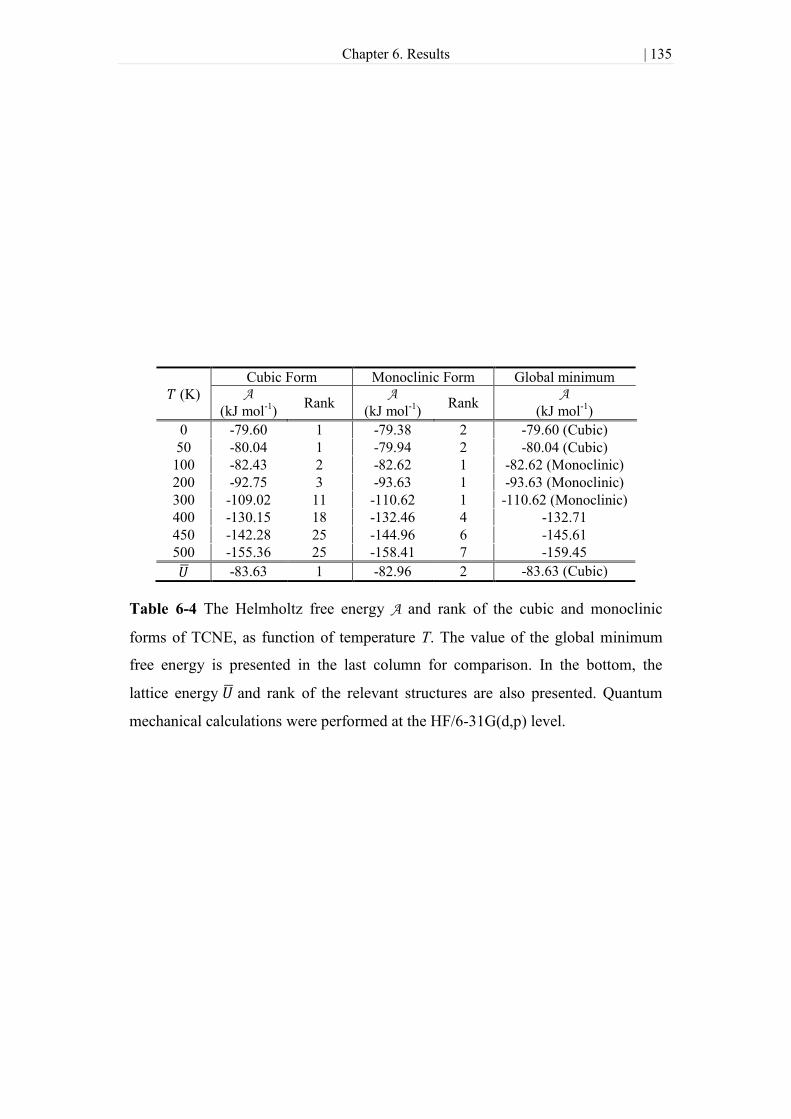
Chapter 6. Results | 135
(K)
Cubic Form Monoclinic Form Global minimum A
(kJ mol-1
) Rank
A
(kJ mol-1
) Rank
A
(kJ mol-1
)
0 -79.60 1 -79.38 2 -79.60 (Cubic)
50 -80.04 1 -79.94 2 -80.04 (Cubic)
100 -82.43 2 -82.62 1 -82.62 (Monoclinic)
200 -92.75 3 -93.63 1 -93.63 (Monoclinic)
300 -109.02 11 -110.62 1 -110.62 (Monoclinic)
400 -130.15 18 -132.46 4 -132.71
450 -142.28 25 -144.96 6 -145.61
500 -155.36 25 -158.41 7 -159.45
-83.63 1 -82.96 2 -83.63 (Cubic)
Table 6-4 The Helmholtz free energy A and rank of the cubic and monoclinic
forms of TCNE, as function of temperature T. The value of the global minimum
free energy is presented in the last column for comparison. In the bottom, the
lattice energy and rank of the relevant structures are also presented. Quantum
mechanical calculations were performed at the HF/6-31G(d,p) level.

Chapter 6. Results | 136
(a)
(b)
Figure 6-17 The Helmholtz free energy landscape of tetracyanoethylene at (a) 0 K ;
(b) 50 K. All necessary quantum mechanical (charge density and geometry)
calculations were performed at HF/6-31G(d,p) level. The colour scale describes the
difference in the rank of each structure before and after the vibrational contributions
are included.

Chapter 6. Results | 137
(a)
(b)
Figure 6-18 The Helmholtz free energy landscape of tetracyanoethylene at (a) 100 K
; (b) 200 K. All necessary quantum mechanical (charge density and geometry)
calculations were performed at HF/6-31G(d,p) level. The colour scale describes the
difference in the rank of each structure before and after the vibrational contributions
are included.

Chapter 6. Results | 138
(a)
(b)
Figure 6-19 The Helmholtz free energy landscape of tetracyanoethylene at (a) 300 K
; (b) 400 K. All necessary quantum mechanical (charge density and geometry)
calculations were performed at HF/6-31G(d,p) level. The colour scale describes the
difference in the rank of each structure before and after the vibrational contributions
are included.

Chapter 6. Results | 139
(a)
(b)
Figure 6-20 The Helmholtz free energy landscape of tetracyanoethylene at (a) 450 K
(b) 500 K. All necessary quantum mechanical (charge density and geometry)
calculations were performed at HF/6-31G(d,p) level. The colour scale describes the
difference in the rank of each structure before and after the vibrational contributions
are included.

Chapter 6. Results | 140
Figure 6-22 The free energy difference between the structure that corresponds to the
monoclinic form and structure #24 as a function of temperature. The red dashed line is a
linear interpolation of the free energy difference in the region of temperatures between
60K and the melting point. The transition temperature is obtained as solution of the
equation on the plot setting y to 0.
Figure 6-21 The free energy difference between the cubic and monoclinic forms of
TCNE as function of temperature. The red dashed line is a linear interpolation of the
free energy difference in the region of temperatures between 60K and the melting point.
The transition temperature is obtained as the solution of the equation on the plot, setting
y to 0.

Chapter 6. Results | 141
6.4.5. The effect of the molecular model on the lattice energy
calculation
In this section the effect of the choice of level of theory for the quantum
mechanical calculations and on the free energy landscapes is investigated.
Calculations are performed using the M06 functional with a 6-31G(d,p) basis set. In
order to perform a free energy calculation under the harmonic approximation, it is
necessary for the structure to be a minimum of the corresponding model. As a
consequence each of the structures of the lattice energy landscape obtained during the
search stage described in section 6.4.2 is minimised again with DMACRYS but the
distributed multipoles and the geometry of the molecules in the gas phase are obtained
at the M06/6-31G(d,p) level and the multipole moments to be used are derived again
at the new level of theory. Following the minimization of 200 structures, 151 unique
structures were obtained, 123 with =1, 27 with =2 and 1 with =8.
The lattice energy landscape obtained is shown in Figure 6-24. The structure
corresponding to the cubic form is ranked second while the monoclinic form
corresponds to the 6th
predicted structure. The cubic form structure is reproduced with
an rms15 equal to 0.103Å, while the monoclinic form is predicted with an rms15 equal
to 0.299Å. While the structure of the monoclinic form is reproduced with similar
accuracy to the HF calculation, the reproduction of the structure of the cubic form is
significantly worse, although still within acceptable limits. An overlay of the
experimental and predicted structures is shown in Figure 6-23. The significantly better
reproduction of the structure of the cubic polymorph and its stabilization with the HF
level of theory may be due to the way in which the Buckingham potential parameters
were derived. The parameters were fitted to reproduce a number of experimental
azahydrocarbon structures using a model based on atomic point charges, where the
atomic point charges had been fitted to reproduce the HF-derived electrostatic
potential around the molecules (Williams & Cox, 1984). In addition, one of the
structures to which the potential parameters were fitted is the cubic polymorph of
TCNE. It can thus be expected that the cubic form of TCNE is best reproduced using
HF. A comparison of the predicted unit cells of the monoclinic and cubic forms at the
M06 and HF levels is found in Table 6-5.
The dispersion curves are once again calculated for the monoclinic form only.
The full set of dispersion curves is shown in Figure 6-25. The external modes are

Chapter 6. Results | 142
compared with the experimental data (Chaplot et al., 1983). The comparison is shown
in Figure 6-26 (the 8 lowest energy modes) and in Figure 6-27 (the remaining four
modes). Qualitatively, the dispersion curves obtained are practically the same as those
obtained using the HF level of theory. The absolute values of the frequencies are
significantly different, however. For example the highest energy mode in the HF level
Figure 6-24 Final lattice energy landscape of TCNE. Red dot and diamond represent
the monoclinic and cubic experimentally known forms. Quantum mechanical
calculation were performed at M06/6-31G(d,p) level.
Figure 6-23 Overlay of the predicted and experimental forms of TCNE. a) the cubic
form matches the experimental with an rms15=0.103Å, b) the predicted monoclinic
form matches the experimental form with an rms15=0.299Å. Quantum mechanical
calculations were performed at the M06/6-31G(d,p) level of theory.

Chapter 6. Results | 143
Form Space
group
QM
level Z a (Å) b (Å) c (Å) β (
o) γ (
o)
π
( g cm-3
)
Cubic HF 18 13.82 13.82 16.94
90 120 1.364
M06 18 13.97 13.97 17.11 1.324
Monoclinic P21 HF 2 6.74 6.00 7.86 80.87
90 1.355
P21 M06 2 6.76 6.05 7.95 80.83 1.326
Table 6-5 Comparison of the unit cells of the two predicted forms of TCNE at M06
and HF level of theory. Lattice angle α is equal to 90o for all forms because of
symmetry constraints.
of theory has a frequency of 79.02 THz while at the M06 level of theory, the
frequency obtained is 71.38 THz.
The comparison of the computed external modes of the monoclinic form with
the available experimental results shows a deterioration in the agreement when
moving to the M06 functional. This effect is more obvious for the lowest 4 modes.
That can be attributed partly in the change of the level of theory for quantum
mechanical calculations and the fact that the minimum obtained at the M06 level is
not identical to the minimum obtained at the HF level.
The free energy landscape is again calculated in the same way it was
calculated for the HF/6-31G(d,p) level (see section 6.4.4), again for the temperature
range 0 K to 500 K. The landscapes for temperatures 0 K, 100 K, 200 K and 300 K
are shown in Figure 6-28 and Figure 6-29. The general qualitative observations
regarding the free energy landscapes at the HF level (see section 6.4.4) are equally
applicable. The variation of the free energy and rank as a function of temperature for
the two polymorphs and that of the global minimum are summarized in Table 6-6, and
several differences are evident from this table.
In contrast to the calculations at the HF/6-31G(d,p) level of theory, the cubic
form here is never predicted as the thermodynamically most stable structure.
Furthermore, the cubic form is predicted to be less dense than the monoclinic form
when using the M06 functional, in contrast to the experimental result. For a wide
range of temperatures (up to approximately 100 K) it remains one of the most stable
structures and is ranked within the 5 lowest free energy structures. The most stable
structure in the low temperature range corresponds to the third-ranked structure on the
HF lattice energy landscape (with an rms15=0.105Å), and is hereafter referred to as
. The transition from this postulated structure to the monoclinic form occurs at

Chapter 6. Results | 144
(K)
Cubic Form Monoclinic Form Global minimum A
(kJ mol-1
) Rank
A
(kJ mol-1
) Rank
A
(kJ mol-1
)
0 -71.87 3 -71.62 6 -72.11
50 -72.39 3 -72.26 5 -72.68
100 -75.06 4 -75.21 2 -75.45
200 -86.28 10 -87.07 1 -87.07 (Monoclinic)
300 -103.70 18 -105.16 4 -110.62
400 -126.15 24 -128.28 8 -132.71
450 -138.99 26 -141.46 10 -145.61
500 -152.80 30 -155.62 10 -159.45
-75.84 2 -75.19 6 -75.17
Table 6-6 The Helmholtz free energy A and rank of the cubic and monoclinic
forms of TCNE, as function of temperature T. The value of the global minimum
free energy is presented in the last column for comparison. In the bottom, the
lattice energy and rank of the relevant structures are also presented. Quantum
mechanical calculations were performed at the M06/6-31G(d,p) level.
163 K, while the cubic form becomes less stable than the monoclinic form at a
temperature of 79.5K, which is very close to the value we calculated using the HF
level. Finally, in the region between 276 K and the melting point, another structure is
stabilized over the monoclinic form. It is the same structure as that was predicted
to be stable at high temperatures at the HF level of theory (within rms15=0.066Å). The
transition temperatures reported here are determined by linear interpolation, in the
same way as in section 6.4.4.
The results obtained using this level of theory are to a large extent different
from the results obtained using the HF level of theory revealing, as expected, the large
degree of dependence of the final result on the chosen computational model. The
choice of functional for the DFT calculations has a pronounced effect on the relative
lattice energy and free energy of the structures. On the other hand the actual structures
obtained are much less sensitive on this choice. Calculations using both functionals
reveal a polymorphic landscape that is dense in structures separated by very small
lattice energy and free energy differences. Although the existence of the high pressure
form cannot be verified by these calculations (performed at 0 atm), the results are
consistent with the puzzling experimental evidence suggesting that at least one more
polymorph may exist. The overall better performance of the HF level of theory may
be due to the fact that a description of the electrostatic potential at this level of theory
was used for the parameterization of the Buckingham potential.

Chapter 6. Results | 145
Figure 6-25 Dispersion curves of TCNE. The 12 lowest energy branches represent
the external modes of vibration while the remaining branches represent the internal
modes. Quantum mechanical calculations were performed at the M06/6-31G(d,p)
level of theory.

Chapter 6. Results | 146
Figure 6-26 Comparison of the 8 experimentally determined lowest frequency
modes of vibration of TCNE (in red) with the corresponding calculated modes (in
black). The wave vector varies along directions , and .
Calculations were carried out at the M06/6-31G(d,p) level of theory.

Chapter 6. Results | 147
Figure 6-27 Comparison of the 4 experimentally determined highest frequency
external modes of vibration of TCNE (in red) with the corresponding calculated
modes (in black). The wave vector varies along directions , and
. Calculations were carried out at the M06/6-31G(d,p) level of theory.

Chapter 6. Results | 148
(a)
(b)
Figure 6-28 The Helmholtz free energy landscape of tetracyanoethylene at (a) 0 K ;
(b) 100 K. All necessary quantum mechanical (charge density and geometry)
calculations were performed at M06/6-31G(d,p) level. The colour scale describes the
difference in the rank of each structure before and after the vibrational contributions
are included.

Chapter 6. Results | 149
(a)
(b)
Figure 6-29 The Helmholtz free energy landscape of tetracyanoethylene at (a) 200 K
; (b) 300 K. All necessary quantum mechanical (charge density and geometry)
calculations were performed at M06/6-31G(d,p) level. The colour scale describes the
difference in the rank of each structure before and after the vibration contributions
are included.

Chapter 6. Results | 150
6.5. Quasi-harmonic free energy minimisation;
Argon example revisited
In order to investigate the effect of temperature on the structure of the argon fcc
crystal, free energy minimization is performed within the quasi-harmonic
approximation, as described in section 3.8. The necessary integrals for the calculation
of the vibrational part of the Helmholtz free energy (equation 3-33) and the free
energy gradient (equation 3-49) are calculated using the Gauss-Legendre quadrature
(subsection 3.7) by sampling 512 wave vectors (8 points for each direction).
The quasi-harmonic approximation is found to provide an accurate estimate of the
effect of temperature on the structure of argon. In Figure 6-30 the lattice constant of
the face centred cubic unit cell fcc of argon is plotted as function of temperature. This
quantity is related to the lattice length of the primitive unit cell αp which is obtained
by the minimization via the relation:
fcc αp (6-1)
The lattice constant fcc compares very well with the experimental values (Berrett &
Jones, 1964; Dobbs et al., 1956; Dobbs & Jones, 1957; Peterson et al., 1966) up to 50
K and the error is satisfactorily low for 15 to 20 K beyond this temperature. This
corresponds to a temperature range that is more than half the melting point. A similar
behavior is observed for the coefficient of thermal expansion :
fcc fcc
fcc (6-2)
The coefficient is shown in Figure 6-31. For the thermal expansion coefficient
there are one set of experimental data (Peterson et al., 1966). For comparison reasons
equation (6-2) is used to convert the experimentally available lattice constants
presented in Figure 6-30 to the coefficient . For that conversion the value for
fcc accepted by each author was used. Good agreement is observed at low
temperatures, and the computational model tends to overestimate the extent of the
variation. It is reasonable to expect that an adjustment of the Lennard-Jones potential

Chapter 6. Results | 151
parameters would allow an even better representation of the temperature dependence
of the geometry of the lattice.
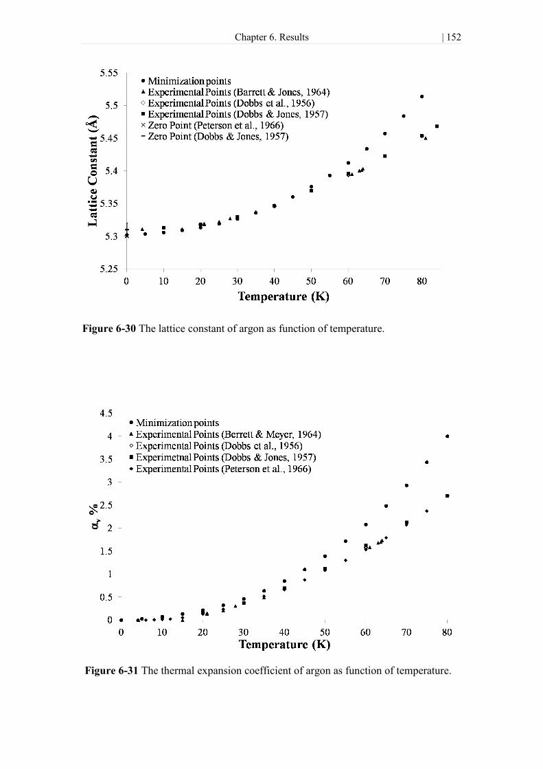
Chapter 6. Results | 152
Figure 6-31 The thermal expansion coefficient of argon as function of temperature.
Figure 6-30 The lattice constant of argon as function of temperature.

Chapter 7. Conclusion and Perspectives | 153
7. Conclusion and Perspectives
7.1. Summary
A method for the incorporation of temperature effects in crystal structure
prediction has been described. The interaction potential of the crystal is approximated
via a Taylor series expansion truncated at second order. The approximate potential
allows the analytical solution of Newton‘s equations of motion, in the general form of
a harmonic plane wave. The indeterminate parameters of the harmonic wave equation
i.e. the frequency of atomic vibrations, and the amplitude of the wave can be obtained
as eigenvalues and eigenvectors of the dynamical matrix. The eigenvalues and
eigenvectors are obtained by diagonalization of the dynamical matrix. In this way the
problem of solving Newton‘s equations of motion is reformulated as an eigenvalue
problem. This method, known as the harmonic approximation in lattice dynamics, has
been widely used in the literature, but has not yet found widespread use in crystal
structure prediction.
Once the frequencies of vibration of the atoms within the crystal have been
obtained, the energy states of the crystal can be calculated by using the equations for
the energy states of the quantum harmonic oscillator. An analytical expression for the
total canonical partition function of the crystal can then be formulated. The canonical
partition function is then used within the framework of statistical mechanics in order
to derive an analytical expression for the Helmholtz free energy of the crystal. In a
similar way, the isothermal-isobaric ensemble partition function can also be
constructed and the Gibbs free energy can be obtained. Under the widely used
assumption of an infinite periodic crystal, the resulting free energy expressions take
an integral form. The efficient evaluation of this integral plays a decisive role in

Chapter 7. Conclusion and Perspectives | 154
determining the computational cost of the method. The main obstacle to overcome
then is the non-trivial task of calculating the dynamical matrix.
The formalism of the harmonic approximation is applicable to any choice of
computational model. Long experience has shown that an accurate representation of
the crystalline solid state requires very detailed models. The intra-molecular
interactions are typically modeled using ab-initio methods. In order to manage the
computational cost of the structure search in a crystal prediction study, such
calculations are often performed for isolated molecules, ignoring the effects of the
crystalline environment. The electrostatic interactions between the molecules are
calculated using multipole expansions truncated at the fourth order. Atomic multipole
moments up to hexadecapole are derived based on the ab-initio derived wave
function, by means of a distributed multipole analysis. In such a way, the applicability
of the method is not restricted by the requirement of experimental data, and high
accuracy is maintained. Finally the repulsion and dispersion interactions are modelled
using the semi-empirical Buckingham potential together with transferable sets of
parameters that are available in the literature for the atoms that are most commonly
found in organic compounds. A detailed description of the molecular models used
was presented in Chapter 4 and a major part of the work was dedicated to the
challenge of calculating the dynamical matrix when using such models.
A major implication of the assumption of an infinite periodic crystal on the
dynamical matrix calculations is that the lattice sums (i.e. the sums over all unit cells
of the crystal) that appear in the calculations are infinite series. When these series
exhibit good convergence properties, such as in the case of the repulsion interactions,
the evaluation of lattice sums is trivial. On the other hand, the infinite series
associated with the electrostatic interactions are not only poorly convergent but also in
some cases converge under conditions. A method for the efficient calculation of the
electrostatic contribution to the lattice energy and the dynamical matrix was
developed in Chapter 5, based on a generalization of the method of Ewald.
The method of harmonic approximation was tested for three compounds, starting
with crystalline argon. The crystal was modeled using a Lennard-Jones potential with
parameters from the literature. The structure of the crystal is known to be face-centred
cubic, and calculations were performed for the primitive unit cell of the fcc crystal.
The primitive unit cell contains only one atom, and the lattice angles are known to be
60o. The lattice lengths are equal, and they were determined via lattice energy

Chapter 7. Conclusion and Perspectives | 155
minimization. Dispersion curves were calculated and found to be in excellent
agreement with the experimentally-determined curves at 5 K. The density of
vibrational states was also calculated based on one million randomly sampled wave
vectors. It was found to be in qualitative agreement with other calculated density of
states. The low frequency region (<0.5THZ) of the density of states is found to have a
quadratic form in line with Debye‘s theory.
To assess the potential for the integration of free energy calculations based on the
harmonic approximation in a crystal structure prediction study, the free energy of
computationally-generated crystal structures was calculated at temperatures from
absolute zero to the melting point for two molecules. An ab-initio crystal structure
prediction methodology based on the CrystalPredictor and DMACRYS algorithms
was applied to imidazole and tetracyanoethylene. Both polymorphs of imidazole were
identified as lattice energy minima. The stable α-form was found as the global
minimum while the β-form, which is unstable at ambient pressure, was found a few kJ
mol-1
higher in lattice energy. The free energy was calculated under the harmonic
approximation from 0 K to the melting point using the 64-node Gauss-Legendre
quadrature method for the evaluation of the free energy integrals. The α-form was
found to remain the global minimum for the whole range of temperatures, while the
free energy difference between the β-form and the global minimum increased as
function of temperature. The calculations were performed using M06/6-31G(d,p) and
HF/6-31G(d,p) level for all the necessary quantum mechanical calculations (intra-
molecular interactions, conformation and charge density). The results obtained are
similar for both ab-initio levels of theory and in good agreement with experimental
data.
Similar calculations were carried out for tetracyanoethylene. TCNE is known to
form four crystals, and structural information is available for two of these: the
monoclinic polymorph and the cubic polymorph. Both of these crystals were
predicted as minima of the lattice energy hypersurface (at the HF/6-31G(d,p) and
M06/6-31G(d,p) levels of theory for the quantum mechanical calculations). With the
HF functional, the cubic form was found to be the global minimum, while the second
lowest energy minimum was found to correspond to the monoclinic form. There was a
small energy difference between these two structures. Dispersion curves were
calculated for the monoclinic form, for which experimental data are available. The
calculated dispersion curves compare very well qualitatively with the experimental
Chapter 7. Conclusion and Perspectives | 156
data. The quantitative differences between the experimentally-determined and
calculated dispersion curves were found to be satisfactorily low. The free energy
calculations indicate that a polymorphic phase transition from the cubic to the
monoclinic form occurs at 74 K. As the temperature was further increased the
structure that corresponds to the 24th
lowest lattice energy minimum became stable.
The transition occurred at 368 K and the structure remained the most stable until the
melting point. This result is in qualitative agreement with the experimental evidence,
although there is some uncertainty about the transition temperature.
The effect of the choice of quantum mechanical model was also investigated for
TCNE. In contrast to imidazole, when calculations were performed using the M06/6-
31G(d,p) level of theory the final result was significantly different from the HF
calculations. Although the shape of the dispersion curve remains the same,
quantitatively, the agreement with experimental data deteriorates slightly. In the free
energy landscapes the cubic form was not found to be the most stable at any
temperature. The structure that was found to be the global minimum of the lattice
energy landscape, , remains the most stable up to 163 K, at which temperature the
monoclinic form becomes the most stable. Finally at 276 K the same structure that
was found to be the most stable at high temperatures in the HF/6-31G(d,p) free energy
landscapes, becomes the most stable. The cubic form was found to be a low-energy
form, more stable at 0 K than the monoclinic form, but becoming less stable at 79.5
K.
Finally the effect of temperature on the structure of the Ar crystal was investigated
within the quasi-harmonic approximation. The free energy of the crystal was
minimized within the quasi-harmonic approximation. The necessary integrals for the
free energy and its gradient were calculated using a 512-node Gauss-Legendre
quadrature. The free energy was minimized from 0 K to 80 K, very close to the
melting point of Ar, which is 84 K. The calculated lattice constant is found to be in
excellent agreement with the experimental constant up to 60K. The thermal expansion
coefficient is exactly the same as the experimental for low temperatures and in very
good agreement in the medium temperature range (30 K to 50 K). When the
temperature increases further the calculations deviate from experimental results.
The results in the studies of imidazole and TCNE suggest that vibrational
contributions to the free energy in principle cannot be neglected, especially in cases
such as TCNE. The effect of temperature on the various landscapes is profound.

Chapter 7. Conclusion and Perspectives | 157
Many structures are eliminated as unstable and extensive rearrangement of the
structures can be achieved. Even if the effect of temperature were overestimated
under the harmonic approximation, the small energetic differences among the putative
structures indicate that entropic contributions cannot be ignored. The harmonic
approximation is thus an excellent first estimate of the effect that temperature may
have on putative crystal structures, especially in the low temperature region. Its
relatively small computational cost allows the evaluation of the free energy of a large
number of structures that are described with detailed but computationally-expensive
models. This approach can be applied as a post-processing stage, following a crystal
structure prediction based on already available lattice energy-based algorithms. The
success of the harmonic approximation in the example of Ar, where an accurate and
widely tested model is used, and other reports that are found in the literature (Falter et
al., 1999; Day et al., 2003; Natkanienc et al, 1980; Righini et al., 1980) suggest that
the errors that are observed in the other examples, e.g., in the calculation of dispersion
curves of TCNE, can to a large extent be attributed to the assumptions in the chosen
model, and secondarily, to an-harmonic effects. This is in accordance with the finding
that the choice of level of theory has a large effect on the calculations for TCNE. The
example of the minimisation of the free energy of Ar under the quasi-harmonic
approximation is an encouraging start for a more comprehensive approach to
modeling temperature effects on the structure of predicted crystals.
7.2. Future work
Lattice dynamics under the harmonic approximation has been shown to be a
promising method for the estimation of the effect of temperature on putative crystal
structures. The work presented in this thesis can be the starting point for many other
advances. A few possible avenues of research are presented in this section.
Issues associated with the computational cost of the method were not addressed
in the thesis. The computations reported here are of the order of one hour per structure
on a single processor (usually an Intel Xeon 5150 2.66GHz). The CPU time
consumed can be significantly reduced in one of many ways. A parallel
implementation of the integration algorithm that is used to evaluate the free energy
expression is a natural step that would significantly reduce the computational cost.
Furthermore the symmetry properties of the crystal impose constraints that allow

Chapter 7. Conclusion and Perspectives | 158
much faster evaluation of the dynamical matrix since it is necessary to calculate only
a portion of the complete matrix. The current implementation does not take symmetry
effects into account. Apart from the computational cost associated with the actual
calculation of the dynamical matrix, this would also reduce the time spent on the
evaluation of the second derivatives of lattice energy. An optimization of the relative
computational cost between the direct space sum and the reciprocal sum by means of
the choice of the Ewald convergence parameter can also be carried out. The
computational cost of the evaluation lattice sums can also be reduced by a
factorization of the orientation dependence of distributed multipoles as described by
Leslie (2008). Although in principle not necessary, it is worth investigating the
possible computational cost savings when evaluating the dispersion contribution in an
Ewald-type manner, as has been done by other authors (in‘t Veld et al., 2007; Isele-
Holder et al., 2012)
The reduced computational cost would allow the use more accurate and detailed
models. The effect that the assumption that atomic vibrations have a negligible effect
on the charge density (described in section 4.4.3) is worth investigating. Adding more
terms in the multipole expansion may also facilitate the determination of the correct
relative stability in cases where many predicted crystals are separated by small,
almost indistinguishable, energy and free energy differences. More accurate
repulsion/dispersion potential parameters can also be obtained by fitting to
experimental data for the vibrations in the crystal, e.g., IR spectra. One must also bear
in mind that these parameters were obtained using a specific level of theory, atomic
point charges, and without accounting for any entropic contributions. Thus, the
derivation of a revised set of parameters, taking into account the use of different
levels of theory, more detailed electrostatics, and entropic contributions, may yield
improved agreement with experimental data.
Harmonic free energy calculations were performed for the hypothetical and
experimental crystal structures of two small rigid molecules, imidazole and
tetracyanoethylene. It is necessary to further validate and investigate the method on
other examples. Comparison with other available dispersion curves would allow a
broader understanding of the capabilities and limitations of the method. The
estimation of the effect of temperature on the computationally generated polymorphic
landscapes of other molecules is also necessary for further assessment of the harmonic
approximation. The method can also be extended to other classes of systems that are

Chapter 7. Conclusion and Perspectives | 159
of interest, such as co-crystals, hydrates, and salts. The method also needs to be tested
on molecules of varying size and flexibility.
The structure of the fcc Ar crystal as function of temperature was determined
with satisfactory accuracy up to half the melting point by free energy minimisation
using the quasi-harmonic approximation. This encouraging result suggests that it is
worth extending the method to organic molecular crystals modeled as described in
chapter 4. This can first be done within a rigid-molecule minimization algorithm. In
this way the effect of temperature on the various predicted structures would also be
estimated, in addition to its effect on their relative stability, as obtained within the
harmonic approximation.
In the second chapter a number of methods were discussed in which the harmonic
crystal was used as a reference state for the calculation of free energy differences in
which anharmonic effects are also included. The calculations presented in this thesis
are an excellent basis for calculation of free energy differences using methods such as
the method of Tan et al. (2010) or the method of Hoover et al. (1970).
Although the methodology presented here does not provide a complete account of
the effect of temperature on crystals, it is a step towards a better understanding of the
organic solid state and brings us closer to the overall objective of determining ab-
initio the phase diagram of organic compounds. .
Conference presentations & publication | 160
Conference presentations & publication
M. Vasileiadis, C.S. Adjiman, & C.C. Pantelides, ―Ab initio prediction of crystal
structure and the effect of temperature on the relative stability of enantiotropic
polymorphs‖, AIChE annual meeting, San Francisco, USA, November 2013 - (talk)
M. Vasileiadis, C.S. Adjiman, & C.C. Pantelides, ―Temperature effects in crystal
structure prediction‖, PPEPPD, Iguazu Falls, Argentina, May 2013 - (talk)
M. Vasileiadis, P.G. Karamertzanis, C.S. Adjiman, & C.C. Pantelides, ―Computation
of entropic effects in crystal structures‖, AIChE annual meeting, Pittsburgh, USA,
October/November 2012 - (talk)
M. Vasileiadis, P.G. Karamertzanis, C.S. Adjiman, & C.C. Pantelides, ―Computation
of entropic effects in crystal structures‖, 5th
FOMMS, Mt. Hood, Oregon, USA, July
2012 - (poster)
M. Vasileiadis, A.V. Kazantsev, P.G. Karamertzanis, O. Lyngverg, C.S. Adjiman, &
C.C. Pantelides, ―Ab initio crystal structure prediction; Methodology & applications
to flexible molecules‖, 6th
CF@Bo, Bologna, Italy, January 2012 - (poster)
M. Vasileiadis, A.V. Kazantsev, P.G. Karamertzanis, C.S. Adjiman, & C.C.
Pantelides, ―The polymorphs of ROY: Application of crystal structure prediction
techniques‖, AIChE annual meeting, Minneapolis, USA, October 2011 - (talk)
M. Vasileiadis, P.G. Karamertzanis, C.S. Adjiman, & C.C. Pantelides, ―Towards
lattice dynamics in crystal structure prediction‖, Thermodynamics conference,
Athens, Greece, September 2011 - (short oral presentation/poster)
M. Vasileiadis, A.V. Kazantsev, P.G. Karamertzanis, C.S. Adjiman, & C.C.
Pantelides, ―Polymorph prediction of a challenging molecule‖, CAPE Forum,
Bradford, UK, March 2011 - (talk)
M. Vasileiadis, E. Siougkrou, D.N. Theodorou, ―MC simulation of a polyethylene
melt: Prediction of volumetric properties under negative pressure. Local density-
cavitation.‖, Thermodynamics conference, London, United Kingdom, September
2009 - (poster)

Conference presentations & publication | 161
M. Vasileaidis, A.V. Kazantsev, P.G. Karamertzanis, C.S. Adjiman & C.C.
Pantelides, ―The polymorphs of ROY: application of a systematic crystal structure
prediction technique‖, Acta Cryst., B68, (2012), 677-685

Chapter 8. Bibliography | 162
8. Bibliography
Abraha A., & Williams D.E., ―Spherical and aspherical intermolecular force fields for
sulphur allotropes‖, Inorg. Chem., 38, 19, (1999), 4224-4228
Abramowitz M., & Stegun I.A., ―Handbook of mathematical functions with formulas,
graphs, and mathematical tables‖, Dover Publications, New York, 1972
Aguado A., & Madden P. A., ―Ewald summation of electrostatic multipole
interactions up to the quadrupolar level‖, J. Chem. Phys., 119, 14, (2003), 7471-
7482
Allen M.P., & Tildesley D.J., ―Computer simulation of liquids‖, Clarendon Press,
Oxford, (1987)
Aung S., & Strauss H.L., ―Lattice sum transformations and potential function
expansions in lattice dynamics‖, J. Chem. Phys., 58, 7, (1973), 2737-2745
Avendaño C., & Gil-Villegas A., ―Monte Carlo simulations of primitive models for
ionic systems using the Wolf method‖, Molecular Physics, 104, 9, (2006), 1475-
1486
Baele P.D., ―Acoustic crystal thermodynamic integration method‖, Phys. Rev. E., 66,
(2002), 036132
Báez L.A., & Clancy P., ―Calculation of free energy for molecular crystals by
thermodynamic integration‖, Molecular Physics, 86, 3, (1995:a), 385-396
Báez L.A., & Clancy P., ―Phase equilibria in extended simple point charge ice-water
systems‖, J. Chem. Phys., 103, 22, (1995:b), 9744-9755
Bansil A., ―Special directions in the Brillouin zone‖, Solid State Communications, 16,
(1975), 885-889
Bardwell D.A., Adjiman C.S., Arnautova Y.A., Bartashevich E., Boerrigter S.X.M.,
Braun D.E., Cruz-Cabeza A.J., Day G.M., Della Valle R.G., Desiraju G.R., van
Eijk B.P., Facelli J.C., Ferraro M.B., Grillo D., Habgood M., Hofmann D.W.M.,
Hofmann F., Jose K.V.J., Karamertzanis P.G., Kazantsev A.V., Kendrick J.,
Kuleshova L.N., Leisen F.J.J., Maleev A.V., Misquitta A.J., Mohamed S.,

Chapter 8. Bibliography | 163
Needs R.J., Neumann M.A., Nikylov D., Orendt A.M., Pantelides C.C., Pickard
C.J., Price L.S, Price S.L., Scheraga H.A., van de Streek J., Thakur T.S., Tiwari
S., venuti E., & Zhitkov I.K., ―Towards crystal structure prediction of complex
organic compounds—a report on the fifth blind test‖, Acta Cryst, B67, (2011),
535-551
Barrett C.S., & Meyer L., ―X-Ray diffraction study of solid argon‖, J. Chem. Phys.,
41, 4, (1964), 1078-1081
Bauer J., Spanton S., Henry R., Quick J., Dziki W., Porter W., & Morris J.,
―Ritonavir: An extraordinary example of conformational polymorphism‖,
Pharmaceutical Research, 18, 6, (2001), 859-866
Bayly C.I., Cieplak P., Cornell W.D., & Kollman P.A., ―A well-behaved electrostatic
potential based method using charge restraints for deriving atomic charges: The
RESP model‖, J. Phys. Chem., 97, 40, (1993), 10269-10280
Bazterra V.E., Ferraro M.B., & Facelli J.C., ―Modified genetic algorithm to model
crystal structures: III. Determination of crystal structures allowing simultaneous
geometry relaxation.‖, International Journal of Quantum Chemistry, 96, 4,
(2004), 312-320
Bennett C.H., ―Efficient estimation of free energy differences from Monte Carlo
data‖, J. Comput. Phys., 22, (1976), 245-268
Berendsen H.J.C., Postma J. P.M., van Gusteren W.F., & Hermans J.: in
Intermolecular forces, edited by Pullman B., (1981), Reidel, Dordrecht, 331
Berg B.A., & Neuhaus T., ―Multicanonical ensemble: a new approach to simulate
first-first order phase transitions‖, Phys., Rev. Lett., 68, 1, (1992), 9-12
Berthelot D., Compte rendus hebdomadaires des séances de l‘academie des sciences,
Academie des sciences (Bechelier, Paris), 126, (1898), 1703-1706
Besler B.H., Merz Jr. K.M., & Kolllman P.A., ―Atomic charges derived from
semiempirical methods‖, J. Comput. Chem., 11, 4, (1990), 431-439
Blackman M., ―On the vibrational spectrum of a three-dimensional lattice‖, Proc.
Roy. Soc. Lond. A, 159, (1937), 416-431

Chapter 8. Bibliography | 164
Bladereschi A., ―Mean-value point in the Brillouin zone‖, Phys. Rev. B, 7, 12, (1973),
5212-5215
Bonadeo H., D‘ Alessio E., Halac E., & Burgos E., ―Lattice dynamics,
thermodynamic function, and phase transitions of p-dichloro and 1,2,4,5-
tetrachlorobenzene‖, J. Chem. Phys., 68(10), (1978), 4714-4721
Born M., ―On the stability of crystal lattices. I‖, Proc. Cambridge Phil. Soc., 36, 2,
(1940), 160-172
Born M., & Bradburn M., ―The thermodynamics of crystal lattices II. Calculation of
certain lattice sums occurring in thermodynamics‖, Proc. Cambridge Phil. Soc.,
39, (1943), 104-113
Born M., & Fürth, ―The stability of crystal lattices. III‖, Proc. Cambridge Phil. Soc.,
36, 4, (1940), 454-465
Born M., & Huang K., ―Dynamical theory of crystal lattices‖, Clarendon Press-
Oxford, (1954)
Born M., & Misra R.D., ―On the stability or crystal lattices.IV‖, Proc. Cambridge
Phil. Soc., 36, (1940), 466-478
Born M., & von Kármán Th., ―Über schwingungen in raumgittern‖, Phys. Zeit., 13,
(1912), 297-309
Born M., & von Kármán Th., ―Über die verteilung der eigenschwingungen von
Punktgittern‖, Phys. Zeit., 14, (1913), 65-71
Breneman C.M., & Wiberg K.B., ―Determining atom-centered monopoles from
molecular electrostatic potentials. The need of high sampling density in
formamide conformational analysis‖, J. Comput. Chem., 11, 3, (1990), 361-373
Brillouin L., ―Wave propagation in periodic structures; electric filters and crystal
lattices‖, Dover publications Inc., (1953)
Bródka A., & Grzybowski A., ―Electrostatic interactions in computer simulations of
three-dimensional system periodic in two directions: Ewald-type summation‖, J.
Chem. Phys., 117, (2002), 8208

Chapter 8. Bibliography | 165
Broughton J.Q., & Gilmer G.H., ―Molecular dynamics investigation of the crystal
fluid interface. I., Bulk properties‖, J. Chem. Phys., 79, 10, (1983), 5095-5104
Bruce A.D., Jackson A.N., Ackland G.J., & Wilding N.B., ―Lattice-switch Monte
Carlo method‖, Phys. Rev. E, 61, 1, (2000), 906-919
Bruce A.D., Wilding N.B., & Ackland G.J., ―Free energy of crystalline solids: a
lattice-switch Monte Carlo method‖, Phys. Rev. Lett., 79, 16, (1997), 3002-
3005
Brush S.G., Sahlin H.L., & Teller E., ―Monte Carlo study of a one-component plasma.
I‖, J. Chem. Phys., 45, 6, (1966), 2102-2118
Caldwell R.F., & Klein M.V., ―Experimental and theoretical study of phonon
scattering from simple point defects in sodium chloride‖, Phys. Rev., 158, 3,
(1967), 851-875
Campaña C., Mussard B., & Woo T.K., ―Electrostatic potential derived atomic
charges for periodic systems using a modified error functional‖, J. Chem.
Theory Comput., 5, 10, (2009), 2866-2878
Campeta A.M., Chekal B.P., Abramov Y.A., Meenan P.A., Henson M.J., Shi B.,
Singer R.A., & Horspool K.R., ―Development of targeted polymorph screening
approach for a complex polymorphic and highly solvating API‖, J. Pharm. Sci.,
99, 9, (2010), 3874-3886
Cerutti D.S., & Case D.A., ―Multi-Level Ewald: A hybrid multigrid/Fast Fourier
transform approach to the electrostatic particle-mesh problem‖, J. Chem.
Theory Comput., 6, (2010), 443-458
Cerutti D.S., Duke R.E., Darden T.A., & Lybrand T.P., ―Staggered mesh Ewald: an
extension of the smooth particle-mesh Ewald adding great versatility‖, J. Chem.
Theory Comput., 5, 9, (2009), 2322-2338
Chadi D.J., & Cohen M.L., ―Special points in the Brillouin zone‖, Phys. Rev. B, 8,
12, (1973), 5747-5753
Challacombe M., Schwegler E., & Almlöf J., ―Recurrence relations for calculation of
the Cartesian multipole tensor‖, Chemical Physics Letters, 241, (1995), 67-72

Chapter 8. Bibliography | 166
Chan H.C.S., Kendrick J., & Leusen F.J.J., ―Molecule VI, a benchmark crystal-
structure-prediction sulfonimide: Are its polymorphs predictable?‖, Angew.
Chem. Int. Ed., 50, (2011), 2979-2981
Chaplin T., Price G.D., & Ross N.L., ―Computer simulation of the infrared and
Raman activity of pyrope garnet and assignment of calculated modes to specific
atomic motions‖ American Mineralogist, 83, (1998), 841-847
Chaplot S.L., ―Free energy and the relative stability of the phases of solid
tetracyanoethylene with pressure and temperature‖, Phys. Rev. B, 36, 16,
(1987), 8471-8477
Chaplot S.L., Mierzejewski A., & Pawley G.S., ―The monoclinic structure of
tetracyanoethylene (TCNE), C6N4, at 5, 150 and 295K; Powder diffraction
analysis‖, Acta Cryst., C40, (1984), 663-666
Chaplot S.L., Mierzejewski A., Pawley G.S., Lefebvre J., & Luty T., ―Phonon
dispersion of external and low-frequency internal vibrations in monoclinic
tetracyanoethylene at 5K‖, J. Phys. C: Solid State Phys., 16, (1983), 625-644
Chaplot S.L., & Mukhopadyay R., ―Monoclinic-amorphous-cubic phase transitions in
tetracyanoethylene under high pressure‖, Phys. Rev. B, 33, 7, (1986), 5099-
5101
Chaplot S.L., Pawley G.S., Bokhenkov E.L., Sheka E.F. Dorner B., Kalus J., Jindal
V.K., & Natkaniec I., ―Eigenvectors of low frequency internal phonons in
crystalline anthrcene-d10‖, Chem. Phys., 57, (1981), 407-414
Chekal B.P, Campeta A.M., Abramov Y.A., Feeder N., Glynn P.P., McLaughlin
R.W., Meenan P.A., & Singer R.A., ―The challenges of developing an API
crystallization process for a complex polymorphic and highly solvating system.
Part I‖, Org. Process Res. & Dev., 13, (2009), 1327-1337
Chemburkar S.R., Bauer J., Deming K., Spiwek H., Patel K., Morris J., Henry R.,
Spanton S., Dziki W., Porter W., Quick J., Bauer P., Donaubauer J., Narayanan
B.A., Soldani M., Riley D., & McFarland K., ―Dealing with the impact of
ritonavir polymorphs on the late stages of bulk drug process development‖, Org.
Process Res. Dev., 4, (2000), 413-417

Chapter 8. Bibliography | 167
Chen D.-L., Stern A.C., Space B., & Johnson J.K., ―Atomic charges derived from
electrostatic potentials for molecular and periodic systems‖, J. Phys. Chem. A,
114, (2010), 10225-10233
Chetkina L.A., & Bel‘skiĭ V.K., ―Structures of tetracyanoethylene and its
tricyanovinyl derivatives with intramolecular charge charge transfer: a review‖,
Crystallography Reports, 47, 4, (2002), 581-602
Chipot C., & Luque F.J., ―Fast evaluation of induction energies: a second-order
perturbation theory approach‖, Chem. Phys., Lett., 332, (2000), 190-198
Chirlian L.E., & Francl M.M., ―Atomic charges derived from electrostatic potentials:
A detailed study‖, J. Comput. Chem., 8, 6, (1987), 894-905
Chisholm J.A., & Motherwell S., ―COMPACK: a program for identifying crystal
structure similarity using distances‖, J. Appl. Cryst., 38, (2005), 228-231
Choi Y., Ree T., & Ree F.H., ―Phase diagram of a Lennard-Jones solid‖, J. Chem.
Phys., 99, 12, (1993), 9917-9919
Cochran W., & Pawley G.S., ―The theory of diffuse scattering of X-rays by a
molecular crystal‖, Proc. Roy. Soc. Lond. A, 280, (1964), 1-22
Cohen M.H., & Keffer F., ―Dipolar sums in the primitive cubic lattices‖, Phys. Rev.,
99, 4, (1955), 1128-1134
Conrad P.B., & de Pablo J.J., ―Comparison of histogram reweighting techniques for a
flexible water model‖, Fluid Phase Equilibria, 150-151, (1998), 51-61
Coogan C.K., ―Some simple theorems concerning crystal lattice sums of electric
potential, electric field, and electric filed gradient in crystals‖, Aust. J. Chem.,
20, (1967), 2551-2565
Coombes D.S., Price S.L., Willock D.J., & Leslie M., ―Role of electrostatic
interactions in determining the crystal structures of polar organic molecules. A
distributed multipole study‖, J. Chem. Phys., 100, 18, (1996), 7352-7360
Cornell W.D., Cieplak P., Bayly C.I., Gould I.R., Merz Jr. K.M., Ferguson D.M.,
Spellmeyer D.C., Fox T., Caldwell J.W., & Kollman P.A., ―A second

Chapter 8. Bibliography | 168
generation force field for the simulation of proteins, nucleic acids, and organic
molecules‖, J. Am. Chem. Soc., 117, (1995), 5179-5197
Cowley R.A., Cochran W., Brockhouse B.N., & Woods A.D.B., ―Lattice dynamics of
alkali halide crystals. III. Theoretical‖, Phys. Rev., 131, 3, (1963), 1030-1039
Cox S.R., Hsu L.-Y., & Williams D.E., ―Nonbonded potential function models for
crystalline oxyhydrocarbons‖, Acta Cryst., A37, (1981), 293-301
Craven B.M., McMullan R.K., Bell J.D., & Freeman H.C., ―The crystal structure of
imidazole by neutron diffraction at 20 oC and -150
oC‖, Acta Cryst., B33,
(1977), 2585-2589
Criado A., ―The influence of Coulombic interactions on thermal parameters for
naphthalene and anthracene: a lattice-dynamical approach‖, Acta Cryst., A45,
(1989), 409-415
Criado A. ―Lattice dynamics and thermal parameters in azahydrocarbons‖, Acta
Cryst., A46, (1990), 489-494
Dahl J.P., ―Correction and extension of Evjen‘s method for evaluating crystal
potential by means of lattice sums‖, J. Phys. Chem. Solids, 26, (1965), 33-40
Darden T., Darrin Y., & Pedersen L., ―Particle mesh Ewald: An method
for Ewald sums in large systems‖, J. Chem. Phys., 98, 12, (1993), 10089-10092
Day G.M., ―Current approaches to predicting molecular organic crystal structures‖,
Cryst. Rev., 17, 1, (2011), 3-52
Day G.M., Cooper T.G., Cruz-Cabeza A.J., Hejczyk K.E., Ammon H.L., Boerrigter
S.X.M., Tan J.S., Della Valle R.G., venuti E., Jose J., Gadre S.R., Desiraju
G.R., Thakur T.S., van Eijk B.P., Facelli J.C., Bazterra V.E., Ferraro, V.E.,
Hofmann D.W.M., Neumann M.A., Leusen F.J.J., Jendrick J., Price S.L.,
Misquitta A.J., Karamertzanis P.G., Welch G.W.A., Scheraga H.A., Arnautova
Y.A., Schmidt M.U., van de Streek J., Wolf A.K., & Schweizer B., ―Significant
progress in predicting the crystal structures of small organic molecules—a
report on the fourth blind test‖, Acta Cryst., B65, (2009), 107-125

Chapter 8. Bibliography | 169
Day G.M., Motherwell W.D.S., Ammon H.L., Boerrigter S.X.M., Della Valle R.G.,
Venuti E., Dzyabchenko A., Dunitz J.D., Schweizer B., van Eijk B.P, Erk P.,
Facelli J.C., Bazterra V.E., Ferraro M.B., Hofmann D.W.M., Leusen F.J.J.,
Liang C., Pantelides C.C., Karamertzanis P.G., Price S.L., Lewis T.C., Nowell
H., Torrisi A., Scheraga H.A., Arnautova Y.A., Schmidt M.U., & Verwer P.,
―A third blind test of crystal structure prediction‖, Acta Cryst., B61, (2005),
511-527
Day G.M., Price S.L., & Leslie M., ―Atomistic calculations of phonon frequencies
and thermodynamic quantities for crystals of rigid organic molecules‖, J. Phys.
Chem. B, 107, 39, (2003), 10919-10933
De Launay J. ―Theory of specific head and lattice vibrations‖, Solid state physics, 2,
(1956), 219-304
De Leeuw S.W., Perram J.W., & Smith E.R., ―Simulation of electrostatic systems in
periodic boundary conditions. I. Lattice sums and dielectric constants‖, Proc. R.
Soc. Lond. A. 373, (1980), 27-56
De Wette F.W., Fowler L.H., & Nijboer B.R.A., ―Lattice dynamics, thermal
expansion and specific heat of a Lennard-Jones solid in teh quasi-harmonic
approximation‖, Physica, 54, (1971), 292-304
De Wette F.W., & Schacher G.E., ―The internal field in general dipole lattices‖, Phys.
Rev., 137, 1A, (1965), 78-91
Deem M.W., Newsam J.M., & Sinha S.K., ―The h=0 term in Coulomb sums by the
Ewald transformation‖, J. Phys. Chem., 94, (1990), 8356-8359
Della Valle R.G., Fracassi P.F., Righini R., Califano S., & Walmsley S.H., ―Phonon
dispersion curves and phonon lifetimes in crystalline ammonia‖, Chem. Phys.,
44, (1979), 189-196
Della Valle R.G., Venuti E., & Brillante A., ―Pressure and temperature effects in
lattice dynamics: the case of naphthalene‖, Chem. Phys., 198, (1995), 79-89

Chapter 8. Bibliography | 170
Demontis P., Spanu S., & Suffritti G.B., ―Application of the Wolf method for the
evaluation of Coulombic interactions to complex condensed matter systems:
Aluminosilicates and water‖, J. Chem. Phys., 114, (2001), 7980
Der Chao S., Kress J. D., & Redondo A., ―An alternative multipolar expansion for
intermolecular potential functions‖, J. Chem. Phys., 120, 12, (2004), 5558-
55765
Derenzo S.E., Klintenberg M.K., & Weber M.J., ―Determining point charge arrays
that produce accurate ionic crystal fields for atomic cluster calculations‖, J.
Chem. Phys., 112, 5, (2000), 2074-2081
Deserno M., & Holm C., ―How to mesh up Ewald sums. I. A theoretical and
numerical comparison of various particle mesh routines‖, J. Chem. Phys.,
109,18, (1998), 7678-7693
Desikan S., Parsons Jr. R.L., Davis W.P, Ward J.E., Marshall W.J., & Toma P.H.,
―Process development challenges to accommodate a late-appearing stable
polymorph: A case study on the polymorphism and crystallization of a fast-track
drug development compound‖, Org. Process Res. Dev., 9, (2005), 933-942
Dick B.G. Jr., & Overhauser A.W., ―Theory of the dielectric constants of alkali halide
crystals‖, Phys. Rev., 112, 1, (1958), 90-103
Diemand J., Angélil R., Tanaka K.K., & Tanaka H., ―Large scale molecular dynamics
simulations of homogeneous nucleation‖, J. chem. Phys., 139, (2013), 074309
Dobbs E.R., Figgins B.F., Jones G.O., Piercey D.C., & Riley D.P., ―Density and
expansivity of solid argon‖, Nature, 178, (1956), 483
Dobbs E.R., & Jones G.O., ―Theory and properties of solid argon‖, Rep. Prog. Phys.
20, (1957), 516
Dorner B., Bokhenkov E.L., Chaplot S.L., Kalus J., Natkaniec I., Pawley G.S.,
Schmelzer U., & Sheka E.F., ―The 12 external and the 4 lowest internal phonon
dispersion branched in d10 – anthracene at 12K‖, J. Phys. C: Solid State Phys.,
15 (1982), 2353-2365
Dove M.T., ―Introduction to lattice dynamics‖, Cambridge University Press, (1993)
Chapter 8. Bibliography | 171
Dove M.T., ―Structure and dynamics: an atomic view of materials‖, Oxford
University Press, (2003)
Dunitz J.D., Filippini G., & Gavezzotti A., ―Molecular shape and crystal packing: a
study of C12H12 isomers, real and imaginary‖, Helv. Chim. Acta., 83, (2000),
2317-2335
Dunitz J.D., & Gavezzotti A., ―Attractions and repulsions in molecular crystals: What
can be learned from the crystal structures of condensed ring aromatic
hydrocarboncs?‖, Acc. Chem. Res., 32, (1999), 677-684
Eike D.M., & Maginn E.J., ―Atomistic simulation of solid-liquid coexistence for
molecular systems: application to triazole and benzene‖, J. Chem. Phys., 124,
(2006), 164503
Eike D.M., Brennecke J.F., & Maginn E.J., ―Towards a robust and general molecular
simulation method for computing solid-liquid coexistence‖, J. Chem. Phys.,
122, (2005), 014115
Einstein A. ―Die Plancksche theorie der strahlung und die theorie der spezifischen
wärme‖, Ann. Phys., 22, (1907), 180-190
Epstein J., Ruble R. J., & Craven B.M., ―The charge density in imidazole by X-ray
diffraction at 103 and 293K‖, Acta Cryst., B38, (1982), 140-149
Essmann U., Perera L., Berkowitz M.L., Darden T., Lee H., & Pedersen L.G., ―A
smooth particle mesh Ewald method.‖ J. Chem. Phys., 103, (19), (1995), 8577-
8593
Evjen H.M., ―On the stability of certain heteropolar crystals‖, Phys. Rev., 39, (1972),
675-687
Ewald P.P., Ann. D. Phys., 54, (1917), 519
Ewald P.P., ―Die berenchnung optischer und elektrostatischer gitteropotentiale.‖,
Ann. D. Phys., 64, (1921), 253-287
Ewald P.P., ―Crystal optics for visible light and X-Rays‖, Rev. Mod. Phys., 37, 1,
(1965), 46-56

Chapter 8. Bibliography | 172
Ewald P.P., ―A review of my papers on crystal optics 1912 to 1968‖, Acta Cryst.,
A35, (1979), 1-9
Falter C., Klenner M., Hoffmann G.A., & Schnetgöke F., ―Dipole polarization and
charge transfer effects in the lattice dynamics and dielectric properties of ionic
crystals‖, Phys. Rev. B, 60, 17, (1999), 12051-12060
Fenell C.J., & Gezelter J.D., ―Is Ewald summation still necessary? Pairwise
alternatives to the accepter standard for long-range electrostatics‖, J. Chem.
Phys., 124, (2006), 234104
Ferrenberg A.M., & Swendsen R.H., ―New Monte Carlo technique for studying phase
transitions‖, Phys. Rev. Lett., 61, 23, (1988), 2635-2638
Ferrenberg A.M., & Swendsen R.H., ―Optimized Monte Carlo data analysis‖, Phys.
Rev. Lett., 63,12, (1989), 1195-1198
Filippini G., Gramaccioli C.M., Simonetta M., & Suffritti G.B., ―Lattice-dynamical
applications to crystallographic problems: Consideration of the Brillouin zone
sampling‖, Acta Cryst., A32, (1976), 259-264
Freeman D.L., & Doll J.D., ―Quantum Monte Carlo study of the thermodynamic
properties of argon clusters: The homogenous nucleation of argon in argon
vapour and ―magic number‖ distributions in argon vapor‖, J. Chem. Phys., 82,
(1985), 462
Frenkel D., & Ladd A.J.C., ―New Monte Carlo method to compute the free energy of
arbitrary solids. Application to the fcc and hcp phases of hard spheres‖, J.
Chem. Phys., 81, 7, (1984), 3188-3191
Frenkel D., & Mulder B.M., ―The hard ellipsoid-of-revolution fluid I. Monte Carlo
simulations‖, Molecular Physics, 100, 1, (2002), 201-217
Frenkel D., & Smimt B., ―Understanding molecular simulation‖, Academic Press,
(2002)
Frisch M. J., Trucks G. W., Schlegel H. B., Scuseria G. E., Robb M. A., Cheeseman J.
R., Scalmani G., Barone V., Mennucci B., Petersson G. A., Nakatsuji H.,
Caricato M., Li X., Hratchian H. P., Izmaylov A. F., Bloino J., Zheng G.,
Chapter 8. Bibliography | 173
Sonnenberg J. L., Hada M., Ehara M., Toyota K., Fukuda R., Hasegawa J.,
Ishida M., Nakajima T., Honda Y., Kitao O., Nakai H., Vreven T., Montgomery
Jr. J. A., Peralta J. E., Ogliaro F., Bearpark M., Heyd J. J., Brothers E., Kudin K.
N., Staroverov V. N., Kobayashi R., Normand J., Raghavachari K., Rendell A.,
Burant J. C., Iyengar S. S., Tomasi J., Cossi M., Rega N., Millam J. M., Klene
M., Knox J. E., Cross J. B., Bakken V., Adamo C., Jaramillo J., Gomperts R.,
Stratmann R. E., Yazyev O., Austin A. J., Cammi R., Pomelli C., Ochterski J.
W., Martin R. L., Morokuma K., Zakrzewski V. G., Voth G. A., Salvador P.,
Dannenberg J. J., Dapprich S., Daniels A. D., Farkas O., Foresman J. B., Ortiz
J. V., Cioslowski J. & Fox D. J. (2009), ‗Gaussian 09 Revision C.1‘, Gaussian,
Inc., Wallingford, CT
Fuchizaki K., ―Towards generalization of Ewald sum‖, J. Phys. Soc. Jap., 63, 11,
(1994), 4051-4059
Fuchizaki K., ―Application of the Generalized Ewald method to a molecular system‖,
J. Phys. Soc. Jap., 79, 2, (2010), 024004
Fujii Y., Lurie N.A., Pynn, R., & Shirane G., ―Inelastic neutron scattering from solid
36Ar‖, Phys. rev. B, 10, 8, (1974), 3647-3659
Fukuda I., & Nakamura H., ―Non-Ewald methods: theory and applications to
molecular systems‖, Biophys. Rev., 4, (2012), 161-170
Fukuda I., Kamiya N., Yonezawa Y., & Nakamura H., ―Simple and accurate scheme
to compute electrostatic interaction: Zero-dipole summation technique for
molecular system and application to bulk water‖, J. Chem. Phys., 137, (2012),
054314
Fukuda I., Yonezawa Y., & Nakamura H., ―Molecular dynamics scheme for precise
estimation of electrostatic interaction via zero-dipole summation principle‖, J.
Chem. Phys., 134, (2011), 164107
Funasako Y., Abe K.-i., & Mochida T., ―Thermal properties of
alkyloctamethylferrocenium salts with TFSA and TCNE (TFSA =
bis(trifluoromethylsulfonyl)amide and TCNE = tetracyanoethylene)‖,
Thermochimica Acta, 532, (2012), 78-82

Chapter 8. Bibliography | 174
Gale J.D., ―Analytical free energy minimisation of silica polymorphs‖, J. Phys. Chem.
B, 102, (1998), 5423-5431
Gale J.D., & Rohl A.L., ―The general utility lattice program‖, Molecular Simulation,
29, 5, (2003),291-341
Gdoutos E.E., Agrawal R., & Espinosa H.D., ―Comparison of the Ewald and Wolf
methods for modelling electrostatic interactions in nonwires‖, Int. J. Numer.
Meth. Eng., 84, (2010), 1541-1551
Gellé A. & Lepetit M.-B., ―Fast calculation of the electrostatic potential in ionic
crystals by direct summation method‖, J. Chem. Phys., 128, (2008), 244716
Ghatak A.K., & Kothari L.S., ―An introduction to lattice dynamics‖, Addison-Wesley,
(1972)
Ghelfenstein M., & Szwarc H., ―Raman spectra in molecular solids II. Low frequency
Raman spectroscopy as a means to study phase changes: More about the
―anomalous‖ γ-phase of p-dichlorobenzene‖, Mol. Cryst. Liq. Cryst., 14, 3-4,
(1971), 283-288
Gilat G., & Raubenheimer L.J., ―Accurate numerical method for calculating
frequency-distribution functions in solids‖, Phys. Rev., 144, 2, (1966), 390-395
Goharshadi E.K., Morsali A., & Mansoori G.A., ―A molecular dynamics study on the
role of attractive and repulsive forces in internal energy, internal pressure and
structure of dense fluids‖, Chem. Phys., 331, (2007), 332-338
Goto M., Takezoe H., & Ishikawa K., ―Carrier transport simulation of anomalous
temperature dependence in nematic liquid crystals‖, Phys. Rev. E, 76, (2007),
040701
Grant W.J.C, ―Computation of lattice sums: Generalization of the Ewald method‖,
B.S.T.J., 44, (1965:a), 427-437
Grant W.J.C, ―Computation of lattice sums: Generalization of the Ewald method II‖,
B.S.T.J., 44, (1965:b), 2433-2446

Chapter 8. Bibliography | 175
Gray A.E., Day G.M., Leslie M., & Price S.L, ―Dynamics in crystals of rigid organic
molecules: contrasting the phonon frequencies calculated by molecular
dynamics with harmonic lattice dynamics for imidazole and 5-azauracil‖,
Molecular Physics, 102, 9-10, (2004), 1067-1083
Greengard L., & Rokhlin V., ―A fast algorithm for particle simulations‖, J. Comput.
Phys., 73, (1987), 325-348
Grochola G., ―Constrained fluid λ-integration: Constructing a reversible
thermodynamic path between the solid and the liquid state‖, J. Chem. Phys.,
120, 5, (2004), 2122-2126
Hanke C.G., Price S.L., & Lynden-Bell R.M., ―Intermolecular potentials for
simulation of liquid imidazolium salts‖, Molecular Physics, 99,10, (2001), 801-
809
Hätting C., ―Recurrence relations for the direct calculation of spherical multipole
interaction tensors and Coulomb-type interaction energies‖, Chem. Phys. Lett.,
260, (1996), 341-351
Hawkins J.A., Rittenhouse J.L, Soper L.M., & Rittenhouse R.C., ―Use of the
primitive unit cell in understanding subtle features of the cubic closest-packed
structure‖, J. Chem. Educ., 85, 1, (2008), 90-92
Herbstein F.H., ―Twinned crystals. II. a-1,2:4,5-tetrachlorobenzene‖, Acta Cryst.,
A18, (1965), 997-1000
Herrero C.P., & Ramírez R., ―Configurational entropy of ice from thermodynamic
integration‖, Chem. Phys. Lett., 568-569, (2013), 70-74
Heyes D.M., Barber M., & Clarke J.H.R., ―Molecular dynamics computer simulation
of surface properties of crystalline potassium chloride‖, J. Chem. Soc. Faraday
Trans II., 73, (1977), 1485-1496
Hilfiker R., ―Polymorphism in the pharmaceutical industry‖, (2006), Wiley-VCH:
New York
Hill T.L., ―An introduction to statistical thermodynamics‖, Dover Publications,
(1986), New York

Chapter 8. Bibliography | 176
Hoover W.G., & Ree F.H., ―Use of computer experiments to locate the melting
transition and calculate the entropy in solid phase‖, J. Chem. Phys., 47,12,
(1967), 4873-4878
Hoover W.G., & Ree F.H., ―Melting transition and communal entropy for hard
spheres‖, J. Chem. Phys., 49, 8, (1968), 3609-3617
Hoover W.G., Ross M., Johnson K.W., Henderson D., Barker J.A., & Brown B.C.,
―Soft-sphere equation of state‖, J. Chem. Phys., 52,10, (1970), 4931-4941
Horbenko E.E., Troitskaya E.P., & Chabanenko V.V., ―Lattice dynamics of
cryocrystals at high pressure‖, Low Temp. Phys., 33, 6-7, (2007), 573-577
Houston W.V., ―Normal vibrations of a crystal lattice‖, Rev. Mod. Phys. 20, 1,
(1948), 161-165
Hsu L.-Y., & Williams D.E., ―Intermolecular potential-function models for crystalline
perchlorohydrocarbons‖, Acta Cryst., A36, (1980), 277-281
Hünenberger P.H., ―Lattice-sum methods for computing electrostatic interactions in
molecular simulations‖, AIP Conf. Proc., 492, 17 (1999), 17-83
in‘t Veld P.J., Ismail A., & Grest G.S., ―Application of Ewald summations to long
range dispersion forces‖, J. Chem. Phys., 127, 14, (2007), 144711
Isele-Holder R.E., Mitchell W., & Ismail A.E., ―Development and application of a
particle-particle particle-mesh Ewald method for dispersion interactions‖, J.
Chem. Phys., 137, (2012), 174107
Ismail S.Z., Anderton C.L., Copley R.C.B., Price L.S., & Price S.L., ―Evaluating the
lattice energy landscape in the context of industrial polymorph screening‖,
Cryst. Growth Des., 13(6), (2013), 2396-2406
Jaswal S.S., ―Deformable-ion model and the lattice dynamics of II-IV compounds:
ZnS‖, J. Phys. C: Solid State Phys., 11, (1978:a), 3559-3563
Jaswal S.S., ―Lattice dynamics of CuCl at 4.2 oK‖, Solid State Communications, 27,
10, (1978:b), 969-971

Chapter 8. Bibliography | 177
Jaswal S.S., & Dilly V.D., ―Deformable-ion model and lattice dynamics of 7LiD‖,
Phys. Rev. B, 15, 4, (1977:a), 2366-2370
Jaswal S.S., & Dilly V.D., ―Second order Raman scattering in MgO‖, Solid state
communications, 24, 8, (1977:b), 577-581
Jayaraman S., & Maginn E. J., ―Computing the melting point and thermodynamic
stability of the orthorhombic and monoclinic crystalline polymorphs of the ionic
liquid 1-n-butyl-3-methylimidazolium chloride‖, J. Chem. Phys., 127, (2007),
214504
Kaminsky R.D., ―Monte Carlo evaluation of ensemble averages involving particle
number variations in dense fluid systems‖, J. Chem. Phys., 101, 6, (1994),
4986-4994
Kamiya N., Fukuda I., & Nakamura H., ―Application of the zero-dipole summation
method to molecular dynamics simulations of a membrane protein system‖,
Chem. Phys. Lett., 568-569, (2013), 26-32
Kantorovich L.N., ―Thermoelastic properties of perfect crystals with nonprimitive
lattices. I. General theory‖, Phys. Rev. B, 51, 6, (1995), 3520-3534
Kaplan I.G., ―Intermolecular interactions: physical picture, computational methods,
model potentials‖, Wiley, (2006), Hoboken, NJ
Karamertzanis P.G., Raiteri P., Parrinello M., Leslie M., & Price S.L., ―The thermal
stability of lattice-energy minima of 5-fuorouracil: Metadynamics as an aid to
polymorph prediction‖, J. Phys. Chem. B., 112, (2008), 4298-4308
Karamertzanis P.G., ―Prediction of crystal structure of molecular solids‖, Ph.D.
Thesis, Imperial College London, (2004)
Karamertzanis P.G., & Pantelides C.C., ―Optimal site charge models for molecular
electrostatic potentials‖, Molecular Simulation, 30, 7, (2004), 413-436
Karamertzanis P.G., & Pantelides C.C., ―Ab-initio Crystal Structure Prediction—I.
Rigid Molecules‖, J. Comput. Chem., 26, 3, (2005), 304-323

Chapter 8. Bibliography | 178
Karamertzanis P.G., & Pantelides C.C., ―Ab-initio Crystal Structure Prediction—II.
Flexible Molecules‖, Molecular Physics, 105, 2-3, (2007), 273-291
Karamertzanis P.G., & Price S.L., ―Energy minimization of crystal structures
containing flexible molecules‖, J. Chem. Theory Comput., 2, (2006), 1184-1199
Karo A.M., & Hardy J.R., ―Precise vibrational frequency distributions and the
second-order Raman spectrum and specific heat of NaCl‖, Phys. Rev., 141, 2,
(1966), 696-710
Kawata M., & Nagashima U., ―Particle mesh Ewald method for three-dimensional
systems with two-dimensional periodicity‖, Chem. Phys. Lett., 340, (2001),
165-172
Kazantsev A.V., Karamertzanis P.G., Adjiman C.S., & Pantelides C.C.,
―CrystalOptimizer: An efficient algorithm for lattice energy minimisation of
organic crystals using quantum mechanical calculations‖, Molecular Systems
Engineering, (2010), edited by C.S. Adjiman & A. Galindo. Germany: Wiley-
VCH
Kazantsev A.V., Karamertzanis P.G., Adjiman C.S., & Pantelides C.C., ―Efficient
handling of molecular flexibility in lattice energy minimization of organic
crystals‖, J. Chem. Theory Comput., 7, 6, (2011: a), 1998-2016
Kazantsev A.V., Karamertzanis P.G., Adjiman C.S., Pantelides C.C., Price S.L.,
Galek P.T.A., Day G.M., & Cruz-Cabeza A.J., ―Successful prediction of a
model pharmaceutical in the fifth blind test of crystal structure prediction‖, Int.
J. Pharmaceuticals, 418, 2, (2011: b), 168-178
Kellermann E.W., ―Theory of the vibrations of the sodium chloride lattice‖, Phil.
Trans. R. Soc. Lond. A, 238, (1940), 513-548
Kellermann E.W., ―On the specific hear of the sodium chloride crystal‖, Proc. Roy.
Soc. A, 178, (1941), 17-24
Kim K.-H., Jung D.H., Kim D., Lee A., Choi K., Kim Y., & Choi S.-H., ―Crystal
structure prediction of organic materials: Tests on the 1,4-diketo-3,6-

Chapter 8. Bibliography | 179
diphenylpyrrolo(3,2-c)pyrrole and 1,4-diketo-3,6-bis(4‘-dipyridyl)-pyrrolo-[3,4-
c]pyrrole‖, Dyes and pigments, 89, 1, (2011), 37-43
Kirkwood J.G., ―Statistical mechanics of fluid mixtures‖, J. Chem. Phys., 3 (1935),
300-313
Kirkwood J.G., ―Critique of the free volume theory of the liquid state‖, J. Chem.
Phys., 18, 3,(1950), 380-382
Kittel C., ―Introduction to solids state physics‖, John Wiley & Sons Inc., (2005),
Kiyohara K., Gubbins K.E., & Panagiotopoulos Z., ―Phase coexistence properties of
polarisable Stockmayer fluids‖, J. Chem. Phys., 106, 8, (1997), 3338-3347
Kofke D.A., ―Direct evaluation of phase coexistence by molecular simulation via
integration along a saturation line‖, J. Chem. Phys., 98, (1993), 4149
Kofke D.A., & Cummings P.T., ―Quantitative comparison and optimization of
methods for evaluating the chemical potential by molecular simulation‖,
Molecular Physics, 92,6, (1997), 973-996
Kofke D.A., & Cummnings P.T., ―Precision and accuracy of staged free-energy
perturbation methods for computing the chemical potential by molecular
simulation‖, Fluid Phase Equilibria, 150-151, (1998), 41-49
Kopsias N.P., & Theodorou D.N., ―Elementary structural transitions in the amorphous
Lennard-Jones solid using multidimensional transition state theory‖, J. Chem.
Phys., 109, 19, (1998), 8573-8582
Kosov D.S., & Popelier P.L.A., ―Atomic partitioning of molecular electrostatic
potentials‖, J. Phys. Chem. A, 104, (2000), 7339-7345
Krylov V.I., ―Approximate calculation of integrals‖, Macmillian, (1962)
Laasonen K., Wonczak S., Strey R., & Laaksonen A., ―Molecular dynamics
simulations of gas-liquid nucleation of Lennard-Jones fluid‖, J. Chem. Phys.,
113, (2000), 9741-9747
Chapter 8. Bibliography | 180
Laino T., & Hutter J., ―Notes on ―Ewald summation of electrostatic multipole
interaction up to quadrupolar level‖ [J. Chem. Phys., 119, 74171, (2003)]‖, J.
Chem. Phys., 129, (2008), 074102
Laio A., & Parrinello M., ―Escaping free energy minima‖, Proc. Nat. Ac. Sci USA,
99, 20, (2002), 12562-12566
Lennard-Jones J.E., ―The equation of state of gases and critical phenomena‖, Physica
IV, (1937), 941-956
Lennard-Jones J.E., & Devonshire A.F., ―Critical phenomena in gases. I‖, Proc. Roy.
Soc. A, 163, (1937), 53-70
LeSar R., Najafabadi R., & Srolovitz D.J., ―Finite-temperature defect properties from
free-energy minimisation‖, Phys. Rev. Lett., 63, 6, (1989), 624-627
Leslie M., ―DL_MULTI—A molecular dynamics program to use distributed
multipole electrostatic models to simulate the dynamics of organic crystals‖,
Molecular Physics, 106, 12-13, (2008), 1567-1578
Little R.G., Pautler D., & Coppens P., ―X-ray structure analysis of cubic
Tetracyanoethylene and the length of the –C N bond. Application of a double-
atom refinement method‖, Acta Cryst., B27, (1971), 1493-1499
Lommerse J.P.M., Motherwell W.D.S., Ammon H.L., Dunitz J.D., Gavezzotti A.,
Hofmann D.W.M., Leusen F.J.J., Mooij W.T.M., Price S.L., Schwizer B.,
Schmidt M.U., van Eijk B.P., Verwer P., Williams D.E., ―A test of crystal
structure prediction of small organic molecules‖, Acta Cryst., B56, (2000), 697-
714
Lorentz H.A., ―Uber die anwendung des statez vom virial in der kinetischen theorie
der gase‖, Ann. Phys., 248, 1, (1881), 127-136
Lu N., & Kofke D.A., ―Optimal intermediates in staged free energy calculations‖, J.
Chem. Phys., 111, 10, (1999), 4414-4423
Luty B.A., Tironi I.G., & van Gunsteren W.F., ―Lattice-sum methods for calculating
electrostatic interactions in molecular simulations‖, J. Chem. Phys., 103, 22,
(1995), 3014-3021

Chapter 8. Bibliography | 181
Luty T., Van Der Avoird A., & Mierzejewski A., ―Lattice dynamics of
tetracyanoethylene‖, Chem. Phys. Lett., 61, 1,(1979), 10-14
Lyubartsev A.P., Martsinovski A.A., Shevkunov S.V., & Vorontsov-Velyaminov
P.N., ―New approach to Monte Carlo calculation of the free energy: Method of
expanded ensembles‖, J. Chem. Phys., 96, 3, (1992), 1776-1783
Madelung E. Phys. Z., (1918), 524
Marathe V.R., Lauer S., & Trautwein A.X., ―Electrostatic potentials using direct-
lattice summations‖, Phys. Rev. B., 27, 8, (1983), 5162-5165
Marsh R.E., ―A refinement of the crystals structure of glycine‖, Acta Cryst. 11,
9,(1958), 654-663
Martinez-Carrera S., ―The crystal structure of imidazole at -150 oC‖, Acta Cryst., 20,
(1966), 783-789
Martoňak R., Laio A., & Parrinello M., ―Predicting crystal structures: The Parrinello-
Rahman method revisited‖, Phys. Rev. Lett., 90, 7, (2003), 075503
Mattei A., & Li T., ―Interplay between molecular conformation and intermolecular
interactions in conformational polymorphism: A molecular perspective from
electronic calculations of tolfenamic acid‖, Int. J. Pharm., 418, (2011), 179-186
Mayo S.L., Olafson B.D., & Goddard W.A., ―DREIDING: A generic force field for
molecular simulations‖, J. Phys. Chem., 94, (1990), 8897-8909
McCrone W.C., ―Polymorphism‖, in ―Physics and chemistry of the organic solid
state‖, vol. 2, edited by Fox D., (1965)
McMullan R.K., Epstein J., Ruble J.R., & Craven B.M., ―The crystal structure of
imidazole at 103K by neutron diffraction‖, Acta Cryst., B35, (1979), 688-691
McQuarrie D.A., ―Statistical Mechanics‖, University Science Books, (2000),
Sausalito, California
McWeeny R., ―Symmetry-introduction to group theory‖, (1963), The international
encyclopedia of physical chemistry and chemical physics, Topic I, Vol. 3.,
edited by: Jones H., Pergamon Press

Chapter 8. Bibliography | 182
Meijer E.J., Frenkel D., LeSar R.A, & Ladd A.J.C., ―Location of melting point at
300K of nitrogen by Monte Carlo simulation‖, J. Chem. Phys., 92, 12, (1990),
7570-7575
Mierzejewski A., & Chaplot S.L., ―Raman scattering study of phase transition in
tetracyanoethylene‖, Conf. Int. Raman. Spectrosc. 7th
(1980), 46-47
Minicozzi W.P., & Stroot M.T., ―Solutions for the indeterminate term occurring in
infinite multipole cubic lattice sums‖, Physica, 51, (1971), 503-508
Misra R.D., ―On the stability of crystal lattices.II‖, Proc. Cambridge Phil. Soc., 36,
(1940), 173-182
Monkhorst H.J., & Pack J.D., ―Special points for Brillouin-zone integrations‖, Phys.
Rev. B, 13, 12, (1976), 5188-5192
Montroll E.W., ―Frequency spectrum of crystalline solids‖, J. Chem. Phys., 10,
(1942), 218-229
Mooij W.T.M., van Eijk B.P., & Kroon J., ―Ab initio crystal structure predictions for
flexible hydrogen-bonded molecules‖, J. Am. Chem. Soc.., 122, (2000), 3500-
3505
Motherwell W.D.S., Ammon H.L., Dunitz J.D., Dzyabchenko A., Erk P., Gavezzotti
A., Hofmann D.W.M., Leusen F.J.J., Lommerse J.P.M., Mooij W.T.M., Price
S.L., Scheraga H., Schweizer B., Schmidt M.U., van Eijk B.P., Verwer P.,
Williams D.E., ―Crystal structure prediction of small organic moleculs: a second
blind test‖, Acta Cryst., B58, (2002), 647-661
Mukhopadhyay R., Chaplot S.L., & Rao K.R., ―Phase transition in
tetracyanoethylene‖, Physica Status Solidi A., 92, (1985), 467-474
Mukhopadhyay R., Deb S.K., Das A., & Chaplot S.L., ―Phase transitions at high
pressure in tetracyanoethylene‖, Solid State Communications, 149, (2009),
1914-1918
Munn R.W., & Luty T., ―Theoretical studies of phase transitions in
tetracyanoethylene‖, Faraday Discuss. Chem. Soc., 69, (1980), 107-114

Chapter 8. Bibliography | 183
Murgich J., & Pissanetzky S., ―Temperature dependence of the 14
N nuclear
quadrupole resonance and the observation of the phase transition in cubic
tetracyanoethylene‖, J. Chem. Phys., 62, (1975), 92-93
Najafabadi R., Srolovitz D.J., & LeSar R., ―Thermodynamic and structural properties
of [001] twist boundaries in gold‖, J. Mater. Res., 6, 5, (1991:a), 999-1011
Najafabadi R., Wang H.Y., Srolovitz D.J., & LeSar R., ―A new method for the
simulation of alloys: Application to interfacial segregation‖, Acta metall.
Mater., 39, 12, (1991:b), 3071-3082
Natkaniec I., Bokhenkov E.L., Dorner B., Kalus J., Mackenzei G.A., Pawley G.S.,
Schmelzer U., & Sheka E.F. ―Phonon dispersion in d8-naphthalene crystal at
6K‖, J. Phys. C: Solid State Phys., 13, (1980), 4265-4283
Nayhouse M., Amlani A.M., & Orkoulas G., ―A Monte Carlo study of the freezing
transition of hard spheres‖, J. Phys.: Condens. Matter, 23, (2011:a), 325106
Nayhouse M., Amlani A.M., & Orkoulas G., ―Precise simulation of the freezing
transition of supercritical Lennard-Jones‖, J. Chem. Phys., 135, (2011:b),
154103
Nayhouse M., Amlani A.M., Heng V.R., & Orkoulas G., ―Simulation of fluid-solid
coexistence via thermodynamic integration using a modified cell model‖, J.
Phys.: Condens. Matter, 24, (2012), 155101
Neto N., Righini R., Califano S., & Walmsley S.H., ―Lattice dynamics of molecular
crystals using atom-atom and multipole-multipole potentials‖, Chem. Phys., 29,
(1978), 167-179
Neumann M.A., & Perrin M.-A., ―Energy ranking of molecular crystals using density
functional theory calculations and an empirical van der Waals correction‖, J.
Phys. Chem. B., 109, (2005), 15531-15541
Nijboer B.R.A., & De Wette F.W., ―On the calculation of lattice sums‖, Physica
XXIII, (1957), 309-321
Nijboer B.R.A., & De Wette F.W., ―The internal field in dipole lattices‖, Physica
XXIV, (1958), 422-431

Chapter 8. Bibliography | 184
Noya E.G., Conte M.M., & Vega C., ―Computing the free energy of molecular solids
by the Einstein molecule approach: Ices XIII and XIV, hard-dumbbells and a
patchy model or proteins‖, J. Chem. Phys., 129, (2008), 104704
Nymand T.M., & Linse P., ―Ewald summation and reaction field methods for
potentials with atomic charges, dipoles and polarizabilities‖, J. Chem. Phys.,
112, (2000), 6152-6160
Oh K.J., & Deng Y., ―An efficient parallel implementation of the smooth particle
mesh Ewald method for molecular dynamics simulations‖, Computer Physics
Communications, 177, (2007), 426-431
Özgen S., Kuzucu V., & Adigüzel, ―Investigation of solid argon crystal by means of
isobaric isoenthalpic MD method‖, Erc. Ünv. Fen. Bil. Derg., 12, 1-2, (1996),
60-74
Paliwoda D., Dziubek K.F., & Katrusiak A., ―Imidazole hidden polar phase‖, Cryst.
Growth Des., 12,9, (2012), 4302-4305
Panagiotopoulos A.Z., ―Direct determination of phase coexistence properties of fluids
by Monte Carlo simulation in a new ensemble‖, Molecular Physics, 61, 4,
(1987), 813-816
Panina N., van de Ven R., Verwer P., Meekes H., Vileg E., & Deroover G.,
―Polymorph prediction of organic pigments‖, Dyes and Pigments, 79, (2008),
183-192
Patel A., Price G.D., & Mendelssohn, M.J., ―A computer simulation of approach to
modelling the structure thermodynamics and oxygen isotope equilibria in
silicates‖, Phys. Chem. Minerals, 17, (1991), 690-699
Pavese A., Catti M., Parker S.C., & A. Wall, ―Modelling of the thermal dependence
of structural and elastic properties of calcite, CaCO3‖, Phys. Chem. Minerals,
23, (1996), 89-93
Pawley G.S., ―Analytic formulation of molecular lattice dynamics based on pair
potential functions‖, Physica Status Solidi B, 49, (1972), 475-488

Chapter 8. Bibliography | 185
Peterson O.G., Batchelder D.N., & Simmons R.O., ―Measurements of X-Ray lattice
constant, thermal expansivity, and isothermal compressibility of argon crystals‖,
Phys., Rev., 150, 2, (1966), 703-711
Pillardy J., Arnautova Y.A., Czaplewski C., Gibson K.D., & Scheraga H.A.,
―Conformation-family Monte Carlo: A new method for crystal structure
prediction‖, PNAS, 98, 22, (2001), 12351-12356
Pillardy J., Wawak R.J., Arnautova Y.A., Czaplewski C., & Scheraga H.A., ―Crystal
structure prediction by global optimization as a tool for evaluating potentials:
role of the dipole moment correction term in successful predictions‖, J. Am.
Chem. Soc., 122, (2000), 907-921
Polson J.M., Trizac E., Pronk S., & Frenkel D., ―Finite-size corrections to the free
energies of crystalline solids‖, J. Chem. Phys., 112, 12, (2000), 5339-5342
Prasad R., & Bansil A. ―Special directions for Brillouin-zone integration: Application
to density-of-states calculations‖, Phys. Rev. B, 21, 2, (1980), 496-503
Press W.H., Teukolsky S.A., Vetterling W.T., & Flannery B.P., ―Numerical recipies:
the art of scientific computing‖, Cambridge University Press, (1986),
Cambridge
Price S.L., ―Computational prediction of organic crystal structures and
polymorphism‖, International Reviews in Physical Chemistry, 27, 3, (2008),
541-568
Price S.L., Leslie M., Welch G.W.A., Habgood M., Price L.S., Karamertzanis P.G., &
Day G.M., ―Modelling organic crystal structures using distributed multipole and
polarizability-based model intermolecular potentials‖, Phys. Chem. Chem.
Phys., 12, (2010), 8478-8490
Price S.L., Patel B., Pridhanani-Jethani P., & Torrisi A., ―Crystal structure prediction
and polymorphism-some mutual insights‖, ACA Transactions, 39, (2004), 2-13
Price S.L., Stone A.J., & Alderton M., ―Explicit formulae for the electrostatic energy,
forces and torques between a pair of molecules of arbitrary symmetry‖, 52, 4,
(1984), 987-1001

Chapter 8. Bibliography | 186
Radomska M., & Radomski R., ―Phase diagrams in the binary systems of
tetracyanoethylene with mesitylene, durene and pentamethylbenzene‖, J.
Therm. Anal., 37, (1991), 693-704
Rafizadeh H.A., & Yip S., ―Lattice dynamics of hexamine—A rigid molecule
approximation‖, J. Chem. Phys., 53, 1, (1970), 315-325
Rahman A., ―Correlations in the motion of atoms in liquid argon‖ Phys. Rev., 136,
2A, (1964), A405-A411
Raiteri P., Martoňak R., & Parrinello M., ―Exploring polymorphism: The case of
benzene‖, Angew. Chem. Int. Ed., 44, (2005), 3769-3773
Ribeiro M.C.C., ―High frequency sound velocity in the glass former
2Ca(NO3)2 3KNO3: Molecular dynamics simulations‖, Phys. Rev. B, 75, 14,
(2007), 144202
Righini R., Califano S., & Walmsley S.H., ―Calculated phonon dispersion curves for
fully deuterated naphthalene crystals at low temperature‖, Chem. Phys., 50,
(1980), 113-117
Righini R., Neto N., Califano S., & Walmsley S.H., ―Lattice dynamics of crystalline
ammonia and deutero-ammonia‖, Chem. Phys., 33, (1978), 345-353
Rudin W., ―Real & Complex analysis‖, McGraw-Hill, (1987)
Salonen M., Napari I., Vehkamäki H., ―Molecular dynamics simulation of atomic
clusters in equilibrium with a vapour‖, Molecular Simulation, 33, 3, (2007),
245-251
Sandler S.I., ―Chemical engineering and thermodynamics‖, John Wiley& Son Inc.,
(1999)
Schatschneider B., Liang J.J., Jezowski S., & Tkatchenko A., ―Phase transition
between cubic and monoclinic polymorphs of the tetracyanoethylene crystal: the
role of temperature and kinetics‖, CrystEngComm, 14, (2012), 4656-4663

Chapter 8. Bibliography | 187
Sepliarsky M., Stachiotti M.G., & Migoni R.L., ―Interface effects in ferroelectric
PbTiO3 ultrathin films on a paraelectric substrate‖, Phys. Rev. Lett., 96, (2006),
137603
Shi W., & Johnson J.K., ―Histogram reweighting and finite-size scaling study of the
Lennard-Jones fluids‖, Fluid Phase Equilibria, 187-188, (2001), 171-191
Sigfridsson E., & Ryde U., ―Comparison of methods for deriving atomic charges from
the electrostatic potential and moments‖, J. Comput. Chem., 19, 4,(1998), 377-
395
Signorini G.F., Righini R., & Schettino V., ―Lattice dynamics of the orthorhombic
phase of KClO4: Ewald‘s method in molecular coordinates‖, Chem. Phys., 154,
(1991), 245-261
Singer K., & Smith W., ―The classical and quantum-mechanical free energy of solid
(Lennard-Jones) argon‖, Chem. Phys. Lett., 140, 4, (1987), 406-410
Smith E.R., ―Electrostatic energy in ionic crystals‖, Proc. R. Soc. Lond. A, 375,
(1981), 475-505
Smith J., MacNamara E., Raftery D., Borchardt T., & Byrn S., ―Application of two-
dimensional 13
C solid-state NMR to the study of conformational
polymorphism‖, J. Am. Chem. Soc., 120, (1998), 11710-11713
Sokalski W.A., & Poirier R.A., ―Cumulative atomic multipole representation of the
molecular charge distribution and its basis set dependence‖, Chem. Phys. Lett.,
98, 1, (1983), 86-92
Sokalski W.A., & Sawaryn A., ―Correlated molecular and cumulative atomic
multipole moments‖, 87, 1, (1987), 526-534
Sokalski W.A., Shibata M., Ornstein R.L., & Rein R., ―Point charge representation of
multicenter multipole moments in calculation of electrostatic properties‖, Theor.
Chim. Acta, 85, (1993), 209
Spackman M.A., ―Potential derived charges using a geodesic point selection scheme‖,
J. Comput. Chem., 17, 1,(1996), 1-18

Chapter 8. Bibliography | 188
Spohr E., ―Effect of electrostatic boundary conditions and system size on the
interfacial properties of water and aqueous solutions‖, J. Chem. Phys., 107,
(1997), 6342-6348
Srivastava U.C., Pandey R.S., & Upadayaya K.S., ―Lattice dynamical study of
potassium bromide using theoretical approach‖, Int. J. Phys. Sci., 5,7, (2010),
972-977
Stone A.J., ―Transformation between Cartesian and spherical tensors‖, Molecular
Physics, 29, 5, (1975), 1461-1471
Stone A.J., ―Properties of Cartesian-spherical transformation coefficients‖, J. Phys. A:
Math. Gen., 9, 4, (1976), 485-497
Stone A.J., ―The description of bimolecular potentials, forces and torques: the S and
V function expansions ‖, Molecular Physics, 36, 1, (1978), 241-256
Stone A.J., ―Distributed multipole analysis, or how to describe a molecular charge
distribution‖, Chem. Phys. Lett., 83, 2, (1981), 233-239
Stone A. J., ―The theory of intermolecular interactions‖, Clarendon Press, Oxford,
(1996)
Stone A.J., ―Distributed multipole analysis: Stability for large basis sets‖, J. Chem.
Theory Comput., 1, 6, (2005:a), 1128-1132
Stone A.J., ―Lattice sums and their derivatives for surface adlayers‖, Molecular
Physics, 103, 18, (2005:b), 2427-2481
Stone A.J., & Alderton M., ―Distributed multipole analysis; Methods and
applications‖, Molecular Physics, 100, 1, (2002), 221-233
Stone A.J., & Tough R.J.A., ―Spherical tensor theory of long-range intermolecular
forces‖, Chem. Phys. Lett., 110, 2, (1984), 123-129
Stroud A.H. ―Gaussian quadrature formulas‖, Prentice-Hall, (1966)
Sutton A.P., ―Temperature-dependent interatomic forces‖, Philosophical Magazine A,
60, 2, (1989), 147-159

Chapter 8. Bibliography | 189
Sutton A.P., Mulheran P.A., & Stoneham A.M., ―Direct free energy minimisation
methods: application to grain boundaries‖, Phil. Trans. R. Soc. Lond. A, 341,
(1992), 233-245
Tan T.B., Schultz A.J., & Kofke D.A., ―Suitability of umbrella- and overlap-
sampling methods for calculation of solid-phase free energies by molecular
simulation‖, J. Chem. Phys., 132, (2010), 214103
Taylor M.B., Barrera G.D., Allan N.L., & Barron T.H.K., ―Free energy derivatives
and structure optimization within quasiharmonic lattice dynamics‖, Phys. Rev.
B, 56, 22, (1997), 14380- 14390
Taylor M.B., Barrera G.D., Allan N.L., Barron T.H.K. & Mackrodt W.C., ―Shell: a
code for lattice dynamics and structure otpimisation of ionic crystals‖, Comput.
Phys. Comm., 109, (1998), 135-143
Theodorou D.N., & Suter U.W., ―Detailed molecular structure of a vinyl polymer
glass‖, Macromolecules, 18, 7, (1985), 1467-1478
Tiwari S.K., Pandey L.K., Shukla L.J., & Upadhyaya K.S., ―van der Walls three body
force shell model (VTSM) for the lattice dynamical studies of thallous
bromide‖, Phys. Scr., 80, (2009), 065603
Tiwari S.K., Shukla L.J, & Upadhyaya K.S., ―Harmonic dynamical behaviour of
thallous halides‖, Pramana—J. Phys., 74, 5, (2010), 793-804
Tkatchenko A., & Scheffler M., ―Accurate molecular van der Waals interaction from
ground-state electron density and free-atom reference data‖, Phys. Rev. Lett.,
102, (2009), 073005
Torrie G.M. & Valleau J.P., ―Monte Carlo free energy estimates using non-Boltzmann
sampling: Application to sub-critical Lennard-Jones fluid‖, Chem. Phys. Lett.,
28, 4, (1974), 578-581
Torrie G.M. & Valleau J.P., ―Nonphysical sampling distributions in Monte Carlo free-
energy estimation: Umbrella sampling‖, J. Comput. Phys., 23, (1977), 187-199
Tough R.J.A., & Stone A.J., ―Properties of the regular and irregular solid harmonics‖,
J. Phys. A., Math. Gen., 10, 8, (1977), 1261-1269

Chapter 8. Bibliography | 190
Toukmaji A.Y., & Board J.A. Jr., ―Ewald summation techniques in perspective: a
survey‖, Computer Physics Communications, 95, (1996), 73-92
Troitskaya E.P., Chabanenko V.V., & Horbenko E.E., ―Nonadiabatic effects in the
lattice dynamics of compressed rare-gas crystals‖, Phys. Sol. State, 47, 9,
(2005), 1748-17584
Troitskaya E.P., Chabanenko V.V., & Horbenko E.E., ―Lattice dynamics in light rare-
gas crystals under pressure‖, Phys. Sol. State, 51, 10, (2009), 2121-2128
Uzoh O.G., Cruz-Cabeza A.J., & Price S.L., ―Is the fenamate group a
polymorphophore? Contrasting the crystal energy landscapes of fenamic acid
and tolfenamic adcids‖, Crys. Growth. Des., 12, 8, (2012), 4230-4239
Valleau J. P., & Card D.N., ―Monte Carlo estimation of the free energy by multistage
sampling‖, J. Chem. Phys., 57, 12, (1972), 5457-5462
Van Der Berg T.H.M., & Van Der Avoird A., ―Analytical two- and three-
dimensional lattice sums for general multipole interactions‖, Chem. Phys. Lett.,
160, 2, (1989), 223-227
van Eijk B.P., ―Ab initio crystal structure predictions for flexible hydrogen-bonded
molecules. Part III. Effect of lattice vibrations‖, J. Comput. Chem., 22, 8,
(2001), 816-826
van Eijk B.P., & Kroon J., ―Coulomb energy of polar crystals‖, J. Phys. Chem. B,
101, (1997), 1096-1100
van Eijk B.P., & Kroon J., ―Comment on ―Crystal structure prediction by global
optimization as a tool for evaluating potentials: role of the Dipole moment
correction term in successful predictions‖‖, J. Chem. Phys. B, 104, (2000),
8089-1100
van Eijk B.P., Mooij W.T.M., & Kroon J., ―Ab initio crystal structure predictions for
flexible hydrogen-bonded molecules. Part II. Accurate energy minimization‖, J.
Comput. Chem., 22, 8, (2001), 805-815

Chapter 8. Bibliography | 191
Vasileiadis M., Kazantsev A.V., Karamertzanis P.G., Adjiman C.S., & Pantelides
C.C., ―The polymorphs of ROY: application of a systematic crystal structure
prediction technique‖, Acta Cryst., B68, (2012), 677-685
Vega C., & Noya E.G., ―Revisiting the Frenkel-Ladd method to compute the free
energy of solids: The Einstein molecule method‖, J. Chem. Phys., 127, (2007),
154113
Vega C., Paras E.P.A., & Monson P.A., ―Solid-fluid equilibria for hard dumbbells via
Monte Carlo simulation‖, J. Chem. Phys., 96, 12, (1992), 9060-9072
Vega C., Sanz E., Abascal J.L.F., & Noya E.G., ―Determination of phase diagrams via
computer simulation: Methodology and applications to water, electrolytes and
proteins‖, J. Phys. Condens. Matter, 20, (2008), 153101
Venkataraman G., & Sahni V.C., ―External vibrations in complex crystals‖, Rev.
Mod. Phys., 42, 4, (1970), 409-470
Viveros-Méndez P.X., & Gil-Villegas A., ―Computer simulation of sedimentation of
ionic systems using the Wolf method‖, J. Chem. Phys., 136, (2012), 154507
Vočadlo L., Wall A., Parker S.C., & Price G.D., ―Absolute ionic diffusion in MgO—
computer simulations via lattice dynamics‖, Physics of the Earth and Planetary
Interiors, 88, (1995), 193-210
Wallace D.C., ―Thermodynamics of crystals‖, Dover Publications, New York, 1972
Wang H., Zhang P., & Schütte C., ―On the numerical accuracy of Ewald, Smooth
Particle Mesh Ewald and Staggered Mesh Ewald methods for correlated
molecular systems‖, J. Chem. Thoery Comput., 8, (2012), 3243-4256
Watson G.N., ―A treatise on the theory of Bessel functions‖, Cambridge University
Press, (1944)
Wedemeyer W., Arnautova Y.A., Pillardy J. Wawak R.J., Czaplewski C., & Scheraga
H.A., ―Reply to ―Comment on ‗Crystal structure prediction by global
opitimization as a tool for evaluating potentials: Role of the dipole moment
correction term in successful predictions‘‖ by B.P. van Eijk and J. Kroon‖, J.
Chem. Phys. B,104, (2000), 8090-8092

Chapter 8. Bibliography | 192
Welch G.W.A., Karamertzanis P.G., Misquitta A.J., Stone A.J., & Price S.L., ―Is the
induction energy important for modelling organic crystals?‖, J. Chem. Theory
Comput., 4, 3, (2008), 522-532
Westacott R.E., & Rodger P.M., ―Full-coordinate free-energy minimisation for
complex molecular crystals: type I hydrates‖, Chem. Phys. Lett., 262, (1996),
47-51
Westacott R.E., & Rodger P.M., ―A local harmonic study of clusters of water and
methane‖, J. Chem. Soc. Faraday Trans., 94, (1998), 3421-3426
White J.A., ―Lennard-Jones as a model for argon and test of extended renormalization
group calculations‖ J. Chem. Phys., 111, 20, (1999), 9352
Whitehead C.E., Breneman C.M., Sukumar N., & Ryan M.D., ―Transferable atom
equivalent multicentered multipole expansion method‖, J. Comput. Chem., 24,
4, (2003), 512-529
Widom B., ―Some topics in the theory of fluids‖, J. Chem. Phys., 39, 11, (1963),
2808-2812
Wilding N.B., and Müller M., ―Accurate measurements of the chemical potential of
polymeric systems by Monte Carlo simulation‖, J. Chem. Phys., 101, (1994),
4324-4330
Williams D.E., ―Failure of net atomic charge models to represent the van der Waals
envelope electric potential of n-alkanes‖, J. Comput. Chem., 15, 7, (1994), 719-
732
Williams D.E., ―Improved intermolecular force field for molecules containing H, C, N
and O atoms with application to nucleoside and peptide crystals‖, J. Comput.
Chem., 22, 11, (2001), 1154-1166
Williams D.E., & Cox S.R., ―Nonbonded potentials for azahydrocarbons: the
Importance of the Coulombic interaction‖, Acta Cryst., B40, (1984), 404-417
Williams D.E., & Houpt D.J., ―Fluorine nonbonded potential parameters derived from
crystalline perfluorocarbons‖, Acta Cryst., B42, (1986), 286-295

Chapter 8. Bibliography | 193
Wolf D., ―Reconstruction of NaCl surfaces from a dipolar solution to the Madelung
problem‖, Phys. Rev. Lett., 68, 22, (1992), 3315-3318
Wolf D., Keblinski P., Phillpot S.R., & Eggebrecht J., ―Exact method for the
simulation of Coulombic systems by spherically truncated, pairwise r-1
summation‖, J. Chem. Phys., 110, 17, (1999), 8254-8282
Woodcock L.V., & Singer K., ―Thermodynamic and structural properties of liquid
ionic salts obtained by Monte Carlo computation. Part 1.-Potassium chloride‖,
Trans. Faraday Soc., 67, (1971), 12-30
Woods A.D.B., Brockhouse B.N., Cowley R.A., & Cochran W., ―Lattice dynamics of
alkali halide crystals. II. Experimental studies of KBr and NaI‖, Phys. Rev.,
131, 3, (1963), 1025-1029
Woods A.D.B., Cochran W., & Brockhouse B.N., ―Lattice dynamics of alkali halide
crystals‖, Phys. Rev., 119, 3, (1960), 980-999
Woods R.J., Khalil M., Pell W., Moffat S.H., & Smith V.H. Jr., ―Derivation of net
atomic charges from molecular electrostatic potentials‖, J. Comput. Chem., 11,
3, (1990), 297-310
Yamawaki H., Aoki K., Kakudate Y., Yoshida M., Usuba S., & Fujiwara S., ―Infrared
study of phase transition and chemical reaction in tetracyanoethylene under high
pressure‖, Chem. Phys. Lett., 198, 1-2, (1992), 183-187
Yamawaki H., Sakashita M., Aoki K., & Takemura K., ―Reversible phase transition
between the metastable phases of tetracyanoethylene under high pressure‖,
Phys. Rev. B, 53, 17, (1996), 11403-11407
Yakub E., & Ronchi C., ―An efficient method for computation of long-ranged
Coulomb forces in computer simulation of ionic fluids‖, J. Chem. Phys., 119,
22, (2003), 11556-11560
Yeh I.-C., & Berkowitz M.L., ―Ewald summation for systems with slab geometry‖, J.
Chem. Phys., 111, 7, (1999), 3155-3162

Chapter 8. Bibliography | 194
Yu L., ―Color changes caused by conformational polymorphism: optical –
crystallography single-crystal spectroscopy, and computational chemistry‖, J.
Phys. Chem. A, 106, (2002), 544-550
Zahn D., Schilling B., & Kast S. M., ―Enhancement of the Wolf damped Coulomb
potential: static, dynamic, and dielectric properties of liquid water from
molecular simulation‖, J. Phys. Chem. B., 106, (2002), 10725-10732
Zare R.N., ―Angular momentum‖, Wiley Interscience, (1988)
Zhang Y., & Maginn E.J., ―A simple AIMD approach to derive atomic charges for
condensed phase simulation of ionic liquids‖, J. Phys. Chem. B, 116, (2012),
10036-10048
Zwanzig R.W., ―High-temperature equation of state by a perturbation method. I.,
Nonpolar gases‖, J. Chem. Phys., 22, 8, (1954), 1420-1426

Appendix A | 195
Appendix A—Relations for the
tensor
The equations obtained using the recurrence relation for the
are reported
here for all the contributions to the electrostatic energy considered in our calculations
for which analytical expressions were not available. These are the charge/quadruple,
quadruple/charge, dipole/dipole, charge/octopole, octopole/charge, dipole/quadruple,
quadruple/dipole, chage/hexadecapole, hexadecapole/charge, octopole/dipole,
dipole/octopole and quadruple/quadruple.
Charge/Quadruple & Quadruple Charge
Dipole/Dipole
Charge/Octopole & Octopole/Charge

Appendix A | 196
Dipole /Quadruple & Quadruple/Dipole
Where
is obtained using the following equations:
Where
is obtained using the following equations:
Charge/Hexadecapole & Hexadecapole/Charge

Appendix A | 197
Dipole/Octopole & Octopole/Dipole
Where
is calculated in the following way:
Where
is calculated in the following way:
Appendix A | 198
Quadruple/Quadruple
Where
and
are calculated as:

Appendix A | 199
The components
and
that are necessary for the calculation of some
components of
are calculated in the following way:
It should be stressed here that the expressions given here are not unique equation
(4-37) gives also other, completely equivalent, expressions for the calculation of the same
.
Appendix B—The term
The calculation of the self correction term
given by equation
(5-34) requires the knowledge of the orientation dependence for all interactions up
second order: charge/charge, charge/dipole, dipole/charge, charge/quadruple,
quadruple/charge and dipole/dipole. While the value of the is known equal to 1
(i.e. there is no orientation dependence for the charge/charge interaction) and
analytical expressions are available for
and
(Price et al., 1984), there
are no available analytical expressions for the second order interactions i.e.
charge/quadruple (
), quadruple/charge (
) and dipole/dipole
.
Those are derived using the ladder operator method (Price et al., 1984) using as
starting points the available analytical expressions for ,
and (Stone,
1978).

Appendix B | 200
Charge/quadruple
Quadruple /Charge
Dipole /Dipole

Appendix B | 201
Using those expressions equation (5-34) can be evaluated and the result is
summarised on the table
0
0
Table 8-1 The self correction term for the different components of the contributions up
to second order to the electrostatic energy hessian (equation 5-34).

Appendix B | 202
0
Table 8-2 The self correction term for the different components of the contributions
from the third order to the electrostatic energy hessian (equation 5-34).