Calculation of Oyster Benefits with a Bioenergetics Model of the Virginia

Oyster

Carl F. Cerco

Environmental Laboratory, US Army Engineer Research and Development Center

April 2014 Draft

Abstract A bioenergetics model is formulated and validated for the Virginia oyster (Crassostrea virginica). The model considers two basic properties of a bivalve population: number of individuals and individual size. Individuals are represented as three energy stores: soft tissue, shell, and reproductive material. The bioenergetics model is coupled to an oyster benefits module. Calculated benefits include various aspects of carbon removal, nitrogen removal, phosphorus removal, solids removal, and shell production. Benefits are calculated for natural mortality and for fisheries harvest. The calculation of benefits is based on mass-balance principles and upon user-supplied values for parameters including resuspension, sediment diagenesis, and dentrification rate. The bioenergetics model is coupled with a representation of the physical environment based on the tidal prism approach and with eutrophication kinetics from the CE-QUAL-ICM model. The bioenergetics model was demonstrated through application to the Great Wicomico River, Virginia, 2000 - 2009. The model provided excellent representation of individual oyster size, of population number, and of average individual age. An overarching conclusion from the application was that representation of the detailed data set collected in this system required corresponding detailed information on recruitment, mortality, and other factors. We concluded that 164 metric tons of carbon per annum was filtered from the water column by oysters and 15.2 tons was buried to deep inactive sediments. An additional 13 metric tons of carbon was buried in the form of shell. Oysters filtered 28 metric tons nitrogen per annum from the Great Wicomico water column. Most was recycled but, ultimately, 6.2 metric tons nitrogen per annum was removed through denitrification and burial of oyster deposits. This nitrogen rate compared favorably with the 18.6 metric tons per annum calculated watershed load of total Kjeldahl nitrogen. The report concludes with recommended next steps. The two foremost recommendations are for additional validation through application to additional systems and for operation with the eutrophication kinetics activated. For further information, contact: Carl F. Cerco, PhD, PE Research Hydrologist, Environmental Laboratory US Army Engineer Research and Development Center Vicksburg MS 39180 601-634-4207 carl.f.cerco@usace.army.mil

Table of Contents Chapter 1. Introduction 1

References 1 Chapter 2. Bivalve Bioenergetics Model 2

References 7 Tables 8 Figures 13 References

Chapter 3. The Tidal Prism Model 18

References 20 Tables 20 Figures 21

Chapter 4. Oyster Benefits 22

References 27 Figures 28

Chapter 5. Application to the Great Wicomico River 33

References 42 Tables 44 Figures 45

Chapter 6. Summary and Conclusions 73

References 77

1 Introduction This document describes the formulation and application of a bivalve bioenergetics model. The first section details the model formulation and parameterization for the Virginia oyster Crassostrea virginica. The bioenergetics model considers energy as its currency and provides advantages for modeling the life cycle of individual organisms. The bioenergetics model described here is derived from a bioenergetics model of the planktivorous fish Brevoortia tyrannus, commonly known as Atlantic menhaden. The menhaden model (Dalyander and Cerco, 2010) was developed as part of the System-Wide Water Resources Program (SWRRP) and is patterned after formulations in the Wisconsin Fish Model (Hanson et al., 1997). A subsequent SWRRP investigation explored the generality of the menhaden bioenergetics approach by adopting the model framework to Virginia oysters. To the greatest extent possible, the model utilized parameters adopted from a mass-balance model of Virginia oysters in Chesapeake Bay (Cerco and Noel, 2005). The description and parameterization provided here are specific to Virginia oysters but the model framework is applicable to a wide range of bivalve filter feeders when provided with appropriate parameter values. The second section of the report describes a newly-developed Oyster Benefits module appended to the bioenergetics calculations. These latter model developments were funded through the (EMRRP). Calculated benefits include nutrient removal (through natural processes and harvesting), shell production, and carbon sequestration. In order to calculate benefits, the bioenergetics and benefits modules are inserted into a simple representation of a tidal embayment. Conditions in the embayment are determined by runoff, tide range, and boundary conditions specified at the head and at the mouth. The report concludes with model application to the Great Wicomico River, a Virginia tributary of the Chesapeake Bay. Computed bivalve biomass and population are compared to observations (Southworth et al., 2010) followed by estimation of oyster benefits. References Cerco, C., and Noel, M. (2005). “Assessing a ten-fold increase in the Chesapeake Bay native

oyster population,” Report to the EPA Chesapeake Bay Program, Annapolis MD. (available at )

Dalyander, P., and Cerco, C. (2010). “Integration of an individual-based fish bioenergetics model

into a spatially-explicit water quality model (CE-QUAL-ICM),” ERDC TN-SWWRP-10-1, US Army Engineer Research and Development Center, Vicksburg MS. (available at )

Hanson, P., Johnson, T., Schindler, D., and Kitchell, J. (1997). “Fish bioenergetics 3.0,” WISCU-

T-97-001, University of Wisconsin Sea Grant Institute, Madison WI. Southworth, M., Harding, J., Wesson, J., and Mann, R. (2010). “Oyster (Crassostrea virginica,

Gmelin 1791) population dynamics on public reefs in the Great Wicomico River, Virginia, USA,” Journal of Shellfish Research 29(2), 271-290.

1

2 Bivalve Bioenergetics Model The Model The model considers two basic properties of a bivalve population: number of individuals and individual size. Individuals are organized in “schools,” a term which originated in the menhaden model which preceded this application (Dalyander and Cerco, 2010). Schools are divided into classes. All individuals in a class share identical characteristics e.g. age and size, but the classes that comprise a school customarily differ in one or more characteristics. Model Description The model considers three stores of energy within the individual oyster (Figure 1). These are shell, soft tissue, and reproductive material. The oysters filter overlying water continuously, although the rate is affected by individual characteristics and by properties of the environment. When the quantity of particulate matter filtered from the water column exceeds the amount the oyster can ingest, the excess is rejected as pseudofeces. The remainder is consumed. A portion of consumption is ejected as feces and excretion. The remainder goes into production of one or more of the energy stores. Soft tissue is lost through respiration, at a rate determined by individual characteristics and by properties of the environment. Two forms of respiration are considered. Active respiration is a constant fraction of the energy expended in feeding. Basal metabolism proceeds at a rate independent of activity. Reproductive material is lost through spawning, which occurs when sufficient reproductive energy is accumulated and when conditions in the environment are appropriate. Number of Individuals The number of individuals in a school is initiated when a school enters the model domain. This conceptualization derives from menhaden, which migrate into and out of Chesapeake Bay. Recruitment is an analogous process that initiates the number of oysters in a school. Subsequently, the number of individuals can only decline due to mortality from four processes: starvation, suffocation, predation, and fishery. The model description is:

∆N = ∆Nstv + ∆Nsuf + ∆Nprd + ∆Nfsh (1) in which: ∆N = number of individuals lost within a model time step ∆Nstv = number of individuals lost to starvation within a model time step ∆Nsuf = number of individuals lost to suffocation within a model time step ∆Nprd = number of individuals lost to predation within a model time step ∆Nfsh = number of individuals lost to fishery within a model time step The number lost to each process is the product of the mortality rate and the number of individuals. In the case of starvation, for example:

2

∆Nstv = Nt⋅ Mstv⋅ ∆t (2) in which: Nt = number of individuals within a class Mstv = mortality rate (time-1) ∆t = model time step A starvation rate of 0.025 day-1 is introduced when the individual weight falls below 50% of the “healthy” weight for that individual. Healthy weight is determined by an allometric relationship:

W = AL ⋅ LBL (3) in which: W = individual weight (g DW) L = individual length (mm) AL, BL = parameters which relate weight and length Mortality due to suffocation is introduced when the dissolved oxygen (DO) concentration falls below 2 g m-3. A maximum mortality rate is multiplied by a logistic function such that the mortality is zero at 2 g m-3 DO and approaches the maximum as DO approaches zero (Figure 2). The functional form and parameter values are adopted from the Chesapeake Bay oyster model (Cerco and Noel, 2005):

Msuf = RD⋅exp 1.1⋅

DOhx − DODOhx − DOqx

1+ exp 1.1⋅DOhx − DO

DOhx − DOqx

(4)

in which: Msuf = mortality rate from suffocation (time-1) RD = mortality rate at zero DO (time-1) DO = dissolved oxygen concentration in overlying water (g m-3) DOhx = DO concentration at which the value of the function is one-half (1.0 g m-3) DOqx = DO concentration at which the value of the function is one-quarter (0.7 g m-3) Mortality rates from predation and fishery are user-specified constants. Bioenergetics The bioenergetics portion of the model determines the size and status of individuals. The bioenergetics model considers energy (quantified in joules) as its currency. Since most conventional environmental models and observations are mass-based, however, conversion between energy and mass is required when employing bioenergetics models with other models or field observations. Our model tracks the energy content, weight, and composition of each oyster school and class. The basic bioenergetics relationship is:

3

dWd t

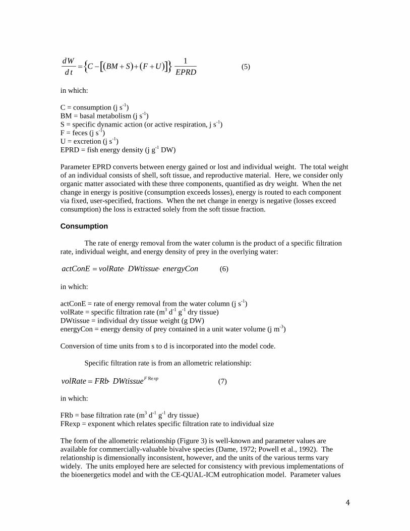
= C − BM + S( )+ F +U( )[ ]{ }⋅1

EPRD (5)

in which: C = consumption (j s-1) BM = basal metabolism (j s-1) S = specific dynamic action (or active respiration, j s-1) F = feces (j s-1) U = excretion (j s-1) EPRD = fish energy density (j g-1 DW) Parameter EPRD converts between energy gained or lost and individual weight. The total weight of an individual consists of shell, soft tissue, and reproductive material. Here, we consider only organic matter associated with these three components, quantified as dry weight. When the net change in energy is positive (consumption exceeds losses), energy is routed to each component via fixed, user-specified, fractions. When the net change in energy is negative (losses exceed consumption) the loss is extracted solely from the soft tissue fraction. Consumption

The rate of energy removal from the water column is the product of a specific filtration rate, individual weight, and energy density of prey in the overlying water:

actConE = volRate⋅ DWtissue⋅ energyCon (6) in which: actConE = rate of energy removal from the water column (j s-1) volRate = specific filtration rate (m3 d-1 g-1 dry tissue) DWtissue = individual dry tissue weight (g DW) energyCon = energy density of prey contained in a unit water volume (j m-3) Conversion of time units from s to d is incorporated into the model code.

Specific filtration rate is from an allometric relationship:

volRate = FRb⋅ DWtissueF Re xp (7) in which: FRb = base filtration rate (m3 d-1 g-1 dry tissue) FRexp = exponent which relates specific filtration rate to individual size The form of the allometric relationship (Figure 3) is well-known and parameter values are available for commercially-valuable bivalve species (Dame, 1972; Powell et al., 1992). The relationship is dimensionally inconsistent, however, and the units of the various terms vary widely. The units employed here are selected for consistency with previous implementations of the bioenergetics model and with the CE-QUAL-ICM eutrophication model. Parameter values

4

are specified such that the filtration rate calculated for a 2 g DWtissue oyster, 0.275 m3 g-1 DW d-

1, agrees with the value derived by Cerco and Noel (2005) from measures conducted in Chesapeake Bay (Jordan, 1987). The volumetric rate determined via Equation 7 is modified to account for effects of temperature, salinity, and suspended solids as per Cerco and Noel (2005).

Prey energy density is patterned after the implementation of the oyster model in the CE-QUAL-ICM eutrophication model. Prey is considered to be the sum of phytoplankton, zooplankton, and detritus, quantified as carbon. A conversion factor is utilized for each prey category to convert from carbon units to energy units. The amount filtered from the water may exceed the rate at which an oyster can ingest material or energy. The maximum ingestion rate is conceived as a fraction of individual weight or energy content per unit time. The fraction is related to individual weight:

fingest = fib⋅ DWtissueing _ exp (8) in which: fingest = ingested fraction (s-1) fib = base ingested fraction (s-1) ing_exp = exponent which relates ingested fraction to individual size The effect of the allometric relationship is to reduce the ingested fraction as an individual increases in size (Figure 4). In the event actConE exceeds the product of the ingested fraction and individual energy content, the excess is rejected as pseudofeces and the remainder is consumption. If ActConE is less than the product of the ingested fraction and individual energy content, the entire amount filtered is consumed. Respiration, Feces, and Excretion Feces are treated as a constant fraction of consumption. Active respiration and excretion are treated as constant fractions of consumption less feces. Basal metabolism is from an allometric relationship that relates specific metabolic rate to individual weight:

RESPCT = BMro⋅ DWtissueBM exp (9) in which: RESPCT = specific metabolic rate (d-1) BMro = base specific metabolic rate (d-1) BMexp = exponent which relates specific metabolism to individual size Parameter values in Equation 9 are specified such that the metabolic rate calculated for a 2 g DWtissue oyster, 0.008 d-1, agrees with the value employed by Cerco and Noel (2005) for Virginia oysters in Chesapeake Bay. The specific metabolic rate is modified to account for temperature and DO as per Cerco and Noel (2005). Specific metabolic rate is converted to energy loss through multiplication by individual weight and energy density:

respireL = RESPCT⋅ DWtissue⋅ EPRD (10)

5

in which: respireL = respiration loss through basal metabolism (j s-1) Conversion of time units from s to d is incorporated into the model code. Energy Gains and Losses The net energy (and equivalent weight) gained or lost must be apportioned to the three compartments: soft tissue, reproduction, and shell. The apportionment is according to a rule set, or decision tree (Figure 5), derived from literature review and model investigation. The rule set is invoked after each discrete time step completed in the numerical integration of Equation 5. The first decision is based on whether energy is gained or lost. Energy loss is removed solely from the soft tissue compartment. The role in respiration of organic material stored in shell and reproduction is unclear and the additional complication of considering energy loss from these components is unwarranted. The allocation of energy (and equivalent weight) gain depends on the health status of the organism, as determined by Equation 3. If the individual is “unhealthy” (tissue weight less than the amount calculated for individual length), all gain goes to soft tissue. If the individual is “healthy” (tissue weight equal to or greater than the amount calculated for individual length), the gain is divided between two or three compartments. A fixed fraction, Fshell, goes to shell organic matter. The fate of the remainder depends on spawning status. If more than six months has passed since the last spawning event, a fixed fraction, Frepro, of the gain not allocated to shell goes to reproduction. The remainder goes to soft tissue. If less than six months has passed since the last spawning event, all gain not allocated to shell goes to soft tissue. Spawning The occurrence of spawning requires simultaneous fulfillment of two criteria:

• The energy stored in reproduction must equal or exceed a specified fraction of the energy stored in soft tissue, and

• Water temperature must equal or exceed a specified value. The criteria for spawning are checked at the completion of each discrete model time step. When these criteria are met, all energy stored in reproduction is released instantaneously and completely. The biomass equivalent of the energy is released to the water column. Due to the unknown fate of the reproductive material, as well as the potential for introduction of larvae from outside the system, recruitment is treated as a model input and is not related to the timing and magnitude of spawning events. Oyster Composition The bioenergetics calculations are based on energy conservation but, when coupled to an environmental model, constituent element mass must be conserved as well. Oyster composition (carbon, nitrogen, phosphorus) is specified in the model parameter set and these elements are cycled between the environment and the organisms as described by Dalyander and Cerco (2010). Under certain environmental conditions, it is possible that consumption of an element relative to growth determined by energy consumption is insufficient to maintain the specified composition.

6

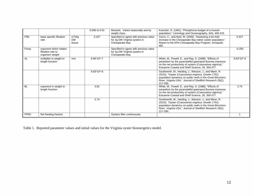
Therefore, elasticity is allowed in composition wherein an oyster can incur an elemental deficit and subsequently retain higher fractions of that element when it is abundant to regain the target composition. Details of this procedure are provided by Dalyander and Cerco (2010). Parameter Values Initial parameter values (Table 1) were selected from published values and from the Cerco and Noel (2005) Virginia oyster model applied to Chesapeake Bay. Initial values were revised and vetted through model simulations of prototype conditions, as described in a subsequent chapter. References Cerco, C., and Noel, M. (2005). “Assessing a ten-fold increase in the Chesapeake Bay native

oyster population,” Report to the EPA Chesapeake Bay Program, Annapolis MD. (available at )

Dalyander, P., and Cerco, C. (2010). “Integration of an individual-based fish bioenergetics model

into a spatially-explicit water quality model (CE-QUAL-ICM),” ERDC TN-SWWRP-10-1, US Army Engineer Research and Development Center, Vicksburg MS. (available at el.erdc.usace.army.mil/elpubs/pdf/swwrp-10-1.pdf )

Dame, R. (1972). “The ecological energies of growth, respiration and assimilation in the intertidal

American oyster Crassostrea virginica,” Marine Biology 17, 243-250. Jordan, S. (1987). “Sedimentation and remineralization associated with biodeposition by the

American oyster Crassostrea virginica (Gmelin),” Ph.D. diss, University of Maryland, College Park.

Powell, E., Hofmann, E., Klinck, J., and Ray, S. (1992). “Modeling oyster populations I. A

commentary on filtration rate. Is faster always better?,” Journal of Shellfish Research 11(2), 387-398.

7

PARM Definition Units Value Notes Reference Initial Model

Value EPLK energy density of

phytoplankton J/g C 54340 Cited by Langefloss and Maurer

(1975) as 5200 cal/g AFDW. Davis, H., and Guillard, R. (1958). “Relative value of ten genera of microorganisms as food for oyster and clam larvae,” Fisheries Bulletin, 136, 293-304.

46000

47700 Converted from cal/mg C using 4.184 J/cal. Mean of 10 values

Platt, T., and Irwin, B. (1973). “Caloric content of phytoplankton,” Limnology and Ocenaography, 18, 306-309

EZOO energy density of zooplankton

J/g C 45000 to 46000 For copepods. Converted from ash-free DW using 0.5 g C/g DW.

Slobodkin, L., and Richman, S. (1961). “Calories/gm in species of animals,” Nature, 4785, 299.

46000

50000 Small copepods. Converted from 5000 J/g WW. Water content is given as 80%

Smith, I., Booker, D., and Wells, N. (2009). “Bioenergetic modeling of the marine phase of Atlantic salmon (Salmo salar L>),” marine Environmental Research, 67, 246-258.

EDET energy density of detritus

J/g C 3600 (winter) to 9200 (summer).

Reported for total seston. Converted to carbon using 0.5 g C/g seston.

Bayne, B., and Worrall, C. (1980). “Growth and production of mussels Mytilus edulis from two populations,” Marine Ecology Progress Series, 3, 317-328.

23000

EPRD predator energy density J/g DW 21800 For mussels. Reported as dry flesh weight.

Bayne, B., and Worrall, C. (1980). “Growth and production of mussels Mytilus edulis from two populations,” Marine Ecology Progress Series, 3, 317-328.

22000

23000 For macoma balthica. Converted from calorie/mg DW

Beukema, J., and de Bruin, W. (1979). “Calorific values of the soft parts of the tellinid bivalve Macoma balthica (L.) as determined by two methods,” Journal of Experimental Marine Biology and Ecology, 37(1), 19-30.

20866 For mussel somatic tissue. Brigolin, D., Dal Maschio, G., Rampazzo, F., Giani, M., and Pastres, R. (2009). “An individual-based population dynamic model for estimating biomass yield and nutrient fluxes through an off-shore mussel (Mytilus galloprovincialis) farm,” Estuarine, Coastal and Shelf Science, 82, 365-376.

21760 For Ostrea edulis. Rodhouse, P. (1978). “Energy transformations by the oyster Ostrea edulis L. in a temperate estuary,” Journal of Experimental Marine Biology and Ecology, 34, 1-22.

fib base value, fraction of filtered material ingested

1/s 1.6*10^-5 For mussels. See July 11 notes Bayne, B., and Worrall, C. (1980). “Growth and production of mussels Mytilus edulis from two populations,” Marine Ecology Progress Series, 3, 317-328.

6.5 * 10^-7

1.4*10^-6 Value used in previous oyster model. See July 11 notes

2.1 to 2.9 * 10^-6 Langefloss, C., and Maurer, D. (1975). “Energy partitioning in the American oyster, Crassostrea virginica (Gmelin),” proceedings of the National Shellfish Association, 65, 20-25.

8

2.2 * 10^-7 For mussels. Brigolin, D., Dal Maschio, G., Rampazzo, F., Giani, M., and Pastres, R. (2009). “An individual-based population dynamic model for estimating biomass yield and nutrient fluxes through an off-shore mussel (Mytilus galloprovincialis) farm,” Estuarine, Coastal and Shelf Science, 82, 365-376.

ing_exp exponent in relationship of ingested fraction to tissue weight

-0.333

BMro base specific metabolic rate

1/d 0.0095 Specified to agree with previous value for 2g DW Virginia oysters in Chesapeake Bay

Cerco, C., and Noel, M. (2005). “Assessing a ten-fold increase in the Chesapeake Bay native oyster population,” Report to the EPA Chesapeake Bay Program, Annapolis MD.

0.0095

exponent which relates metabolic rate to organism weight

Specified to agree with previous value for 2g DW Virginia oysters in Chesapeake Bay

-0.25

RD rate of mortality from suffocation

0.329

SDA fraction of ingestion that goes to specific dynamic action

0.2 Annual average respiration for Macoma Balthica. This combines basal metabolism and SDA.

Hummel, H. (1985). “An energy budget for a Macoma balthica (Mollusca) population living on a tidal flat in the Dutch Wadden Sea,” Netherlands Journal of Sea Research, 19(1), 84-92.

0.2

0.48 Annual respiration for Crassostrea gigas. Combines basal metabolism and SDA.

Kim (1980) cited by Deslous-Paoli, J. “Assessment of energetic requirements of reared molluscs and of their main competitors<’ Laboratoire Aquaculture IFREMER, La Tremblade, France.

0.21 Based on budget that includes feces and pseudofeces. Likely low relative to ingestion. Annual average for 1-year old oyster

Heral, M. “Traditional oyster culture in France” IFREMER. La Tremblade, France.

FA fraction of ingestion that goes to egestion

0.58 Annual average for Macoma balthica. Calculated from stomach contents so this is ingested ration. Pseudofeces not a factor

Hummel, H. (1985). “An energy budget for a Macoma balthica (Mollusca) population living on a tidal flat in the Dutch Wadden Sea,” Netherlands Journal of Sea Research, 19(1), 84-92.

0.5

0.24 Annual average for Crassostrea gigas. Kim (1980) cited by Deslous-Paoli, J. “Assessment of energetic requirements of reared molluscs and of their main competitors<’ Laboratoire Aquaculture IFREMER, La Tremblade, France.

0.74 Includes feces and pseudofeces. Annual average for 1-year old oyster

Heral, M. “Traditional oyster culture in France” IFREMER. La Tremblade, France.

UA fraction of ingestion that goes to excretion

0.05

9

FTISS fraction of assimilation that goes to tissue when time since last spawning event is less than six months

0.75 Annual average for Crassostrea gigas. Kim (1980) cited by Deslous-Paoli, J. “Assessment of energetic requirements of reared molluscs and of their main competitors<’ Laboratoire Aquaculture IFREMER, La Tremblade, France.

0.4

0.55 Annual average or 1-year old oyster Heral, M. “Traditional oyster culture in France” IFREMER. La Tremblade, France.

FSHELL fraction of assimilation that goes to shell

0.3 Dame, R. (1976). “Energy flow in an intertidal oyster population,” Estuarine and Coastal marine Science, 4, 243-253.

0.6

0.02 Annual average for Crassostrea gigas. Kim (1980) cited by Deslous-Paoli, J. “Assessment of energetic requirements of reared molluscs and of their main competitors<’ Laboratoire Aquaculture IFREMER, La Tremblade, France.

0.27 Annual average or 1-year old oyster Heral, M. “Traditional oyster culture in France” IFREMER. La Tremblade, France.

0.1 to 0.3 For mussel. Duarte, P., Fernandes-Reiriz, M., Filgueira, R., Labarta, U. (2010). “Modeling mussel growth in ecosystems wiith low suspended matter loads,” Journal of Sea Research, 64, 273-286.

FREPRO fraction of assimilation, after shell production, that goes to reproduction when time since last spawning event is greater than six months

mean value = 0.2. range = 0.013 to

0.60.

For mussels. Bayne, B., and Worrall, C. (1980). “Growth and production of mussels Mytilus edulis from two populations,” Marine Ecology Progress Series, 3, 317-328.

0.5

0.146 Dame, R. (1976). “Energy flow in an intertidal oyster population,” Estuarine and Coastal marine Science, 4, 243-253.

0.13 Annual average for Crassostrea gigas. 0.18 Annual average or 1-year old oyster Heral, M. “Traditional oyster culture in France” IFREMER. La

Tremblade, France.

0.37 (25C, July to December) to

0.62 (25C, January to June)

Varies with temperature and season. For Crassostrea virginica

Hofmann, E., Klinck, J., Powell, E., Boyles, S., and Ellis, M. (1994). “Modeling oyster populations II. Adult size and reproductive effort,” Journal of Shellfish Research, 13(1), 165-182.

RPRTEMP spawning temperature C 20 actually reported by Bacher & Gangnery, attributed to Pouvreau et al.

Pouvreau, S., Bourles, Y., Lefebvre, S., Gangnery, A., and Alunno-Bruscia, M. (2006). “Application of a dynamic energy budget model to the Pacific oyster, Crassostrrea gigas, reared under various environmental conditions,” Journal of Sea Research, 56, 156-167.

23

10

SPFRAC fraction of reproductive tissue required for spawning

0.04 to 0.15 weight loss calculated for 2.5 g dry body weight. For mussels.

Bayne, B., and Worrall, C. (1980). “Growth and production of mussels Mytilus edulis from two populations,” Marine Ecology Progress Series, 3, 317-328.

0.2

0.35 actually reported by Bacher & Gangnery, attributed to Pouvreau et al.

Pouvreau, S., Bourles, Y., Lefebvre, S., Gangnery, A., and Alunno-Bruscia, M. (2006). “Application of a dynamic energy budget model to the Pacific oyster, Crassostrrea gigas, reared under various environmental conditions,” Journal of Sea Research, 56, 156-167.

AFNM annual rate of natural mortality

0.58 to 0.77 Derived from reported average life span of 6 to 8 years

National Research Council. (2004). “Oyster biology”. Nonnative oysters in the Chesapeake Bay. Committee on Nonnative Oysters in Chesapeake Bay, National Academies Press, Washington DC, 70.

1.2

0.12 to 0.18 Predation rate on Delaware Bay oysters. About half the mortality rate from disease.

Ford, S., and Haskin, H. (1982). “History and epizootiology of Haplosporidium nelsoni (MSX), an oyster pathogen in Delaware Bay, 1957-1980,” Journal of Invertebrate Pathology, 40(1), 118-141. (reference from NRC above, I don’t have original source).

0.1 to 1.0 Annual mortality rate calculated for Great Wicomico River, Virginia

Southworth, M., Harding, J., Wesson, J., and Mann, R. (2010). "Oyster (Crassostrea virginica, Gmelin 1791) population dynamics on public reefs in the Great Wicomico River, Virginia USA," Journal of Shellfish Research 29(2), 217-290.

AFFM annual rate of fishing mortality

0.01

FCDW carbon to dry weight ratio

g C/g DW 0.35 to 0.44 For mussel. Duarte, P., Fernandes-Reiriz, M., Filgueira, R., Labarta, U. (2010). “Modeling mussel growth in ecosystems wiith low suspended matter loads,” Journal of Sea Research, 64, 273-286.

0.5

FNDW nitrogen to dry weight ratio

g N/g DW 0.12 Converted from 0.24 g N/g C Brigolin, D., Dal Maschio, G., Rampazzo, F., Giani, M., and Pastres, R. (2009). “An individual-based population dynamic model for estimating biomass yield and nutrient fluxes through an off-shore mussel (Mytilus galloprovincialis) farm,” Estuarine, Coastal and Shelf Science, 82, 365-376.

0.08

0.09 to 0.12 For mussels. Converted from g N/g C. Duarte, P., Fernandes-Reiriz, M., Filgueira, R., Labarta, U. (2010). “Modeling mussel growth in ecosystems wiith low suspended matter loads,” Journal of Sea Research, 64, 273-286.

FPDW phosphorus to dry weight ratio

g P/g DW 0.01 Converted from 0.02 g P/C Brigolin, D., Dal Maschio, G., Rampazzo, F., Giani, M., and Pastres, R. (2009). “An individual-based population dynamic model for estimating biomass yield and nutrient fluxes through an off-shore mussel (Mytilus galloprovincialis) farm,” Estuarine, Coastal and Shelf Science, 82, 365-376.

0.008

11

0.006 to 0.01 Mussels. Varies seasonally and by weight class.

Kuenzler, E. (1961). “Phosphorus budget of a mussel population,” Limnology and Oceanography, 6(4), 400-415.

FRb base specific filtration rate

m3/d/g DW tissue

0.327 Specified to agree with previous value for 2g DW Virginia oysters in Chesapeake Bay

Cerco, C., and Noel, M. (2005). “Assessing a ten-fold increase in the Chesapeake Bay native oyster population,” Report to the EPA Chesapeake Bay Program, Annapolis MD.

0.327

Frexp exponent which relates filtration rate to organism weight

Specified to agree with previous value for 2g DW Virginia oysters in Chesapeake Bay

-0.250

AL multiplier in weight to length function

mm 8.96*10^-7 White, M., Powell. E., and Ray, S. (1988). “Effects of parasitism by the pyramidellid gastropod Boonea impressa on the net productivity of oysters (Crassostrea viginica),” Estuarine Coastal and Shelf Science, 26, 359-377.

9.63*10^-6

9.63*10^-6 Southworth, M., Harding, J., Wesson, J., and Mann, R. (2010). "Oyster (Crassostrea virginica, Gmelin 1791) population dynamics on public reefs in the Great Wicomico River, Virginia USA," Journal of Shellfish Research 29(2), 217-290.

BL exponent in weight to length function

3.81 White, M., Powell. E., and Ray, S. (1988). “Effects of parasitism by the pyramidellid gastropod Boonea impressa on the net productivity of oysters (Crassostrea viginica),” Estuarine Coastal and Shelf Science, 26, 359-377.

2.74

2.74 Southworth, M., Harding, J., Wesson, J., and Mann, R. (2010). "Oyster (Crassostrea virginica, Gmelin 1791) population dynamics on public reefs in the Great Wicomico River, Virginia USA," Journal of Shellfish Research 29(2), 217-290.

FFRC fish feeding fraction Oysters filter continuously 1

Table 1. Reported parameter values and initial values for the Virginia oyster bioenergetics model.

12

Figure 1. Energy flows in the bivalve energetics model.

13

Figure 2. Modeled effect of dissolved oxygen on filtration and suffocation (mortality) rates.

14

Figure 3. The effect of individual size on specific filtration rate. As an individual increases in size, the filtration rate diminishes. The relationship is calculated for Frexp = -0.25. The same relationship applies to the effect of individual size on specific metabolic rate.

15

Figure 4. The effect of individual size on ingested fraction. As an individual increases in size, the ingested fraction diminishes. The relationship is calculated for ing_exp = -0.333.

16

Figure 5. Allocation of energy gains/losses to energy stores with individual oysters.

17

3 The Tidal Prism Model Introduction Operation of the bioenergetics model requires a description of the surrounding environment – temperature, salinity, dissolved oxygen, and other factors which influence organism growth and mortality. The environmental conditions are typically provided by a detailed predictive model of the system in which the organisms are found. The menhaden bioenergetics model, for example, operates within a Chesapeake Bay model in which the system volume is divided into 4,000 discrete computation cells (Dalyander and Cerco, 2010). The bioenergetics model is modularized and should operate in any system representation including the current 50,000-cell Chesapeake Bay computational grid (Cerco et al., 2010). Model parameterization and calibration are facilitated by operation on a reduced system, however. The oyster bioenergetics model is more likely to find widespread use when application does not require operation of sophisticated hydrodynamic and eutrophication models. To both facilitate and promote model usage, the oyster bioenergetics model is coupled with a basic tidal prism model applicable to tidal rivers and embayments. The tidal prism model considers a single, well-mixed water body (Figure 1). Runoff enters at the head and an equivalent water volume leaves through the mouth. An additional volume, the tidal prism, is exchanged with the external environment through the mouth during every tidal cycle. Runoff carries with it dissolved and particulate materials including suspended solids and nutrients. Material is also exchanged with the external environment through the mouth. The direction of the net exchange, into or out of the system, depends on the relative magnitudes of runoff versus tidal prism and upon relative material concentrations inside and outside the system. The concentration of materials within the system is also influenced by internal sources and sinks. For this application, the only internal sources and sinks considered are oyster uptake and release. More sophisticated representations of transformations in the water column can be added but are left for future developments. The Tidal Prism Model Consider a system as described in the introductory paragraph. The concentration of a dissolved or particulate substance is described:

V ⋅dCdt

= Qin⋅ Cin + Tp⋅ Cb − Tp⋅ C − Qin⋅ C ± S (1)

in which: C = concentration (M L-3) V = volume (L3) Qin = runoff rate (L3 T-1) Cin = concentration in runoff (M L-3) Tp = tidal prism (L3 T-1) S = sum of internal sources and sinks (M T-1) t = time (T) The quantity on the left-hand side of the equation is the rate of change of mass within the system. The quantities on the right hand are the processes which contribute to the change: runoff, import

18

on the incoming tide, loss on the outgoing tide, loss through runoff leaving the system, and internal sources/sinks, respectively. Equation 1 can be rearranged to represent concentration:

dCdt

= −C⋅(Tp + Qin)

V+

Qin⋅ CinV

+Tp⋅ Cb

V±

SV

(2)

In this case, the first term on the right-hand side represents loss through the mouth while the remaining terms represent runoff, import through the mouth, and internal sources/sinks respectively. Summarizing the last three terms on the right gives

dCdt

= −C⋅(Tp + Qin)

V±

S∑V

(3)

Equation 3 can be solved exactly using an integrating factor:

C =S∑

Qin + Tp⋅ 1− exp(−

Qin + TpV

⋅ t)

+ Co⋅ exp(−

Qin + Tp)V

⋅ t) (4)

in which: Co = initial concentration at time t=0 The model advances time in discrete time steps and solves for concentration at time t+∆t as:

Ct +∆t =S∑

Qin + Tp⋅ 1− exp(−

Qin + TpV

⋅ ∆t)

+ Ct ⋅ exp(−

Qin + Tp)V

⋅ ∆t) (5)

in which: ∆t = discrete model time step Model State Variables The tidal prism model accounts for a state variable suite (Table 1) derived from the comprehensive suite in the complete CE-QUAL-ICM model (Cerco et al., 2010). The ICM kinetics are not activated at present. The only internal transformations of state variables occur as a result of oyster uptake and output. This representation is appropriate for a system in which external loads and boundary conditions prevail over local transformation processes.

19

References Cerco, C., Kim, S.-C., and Noel, M. (2010). “The 2010 Chesapeake Bay eutrophication model,”

Report to the US Environmental Protection Agency Chesapeake Bay Program and to the US Army Engineer District Baltimore. (available at http://www.chesapeakebay.net/publications/title/the_2010_chesapeake_bay_eutrophication_model1)

Dalyander, P., and Cerco, C. (2010). “Integration of a fish bioenergetics model into a spatially-

explicit water quality model: Application to menhaden in Chesapeake Bay,” Ecological Modelling 221, 1922-1933.

Table 1 Tidal Prism Model State Variables Salinity Ammonium Temperature Dissolved Organic Nitrogen Suspended Solids Labile Particulate Organic Nitrogen Algal Group 1 (Usually Cyanobacteria) Refractory Particulate Organic Nitrogen Algal Group 2 (Usually Spring Diatoms) Phosphate Algal Group 3 Dissolved Organic Phosphorus Mesozooplankton Labile Particulate Organic Phosphorus Dissolved Organic Carbon Refractory Particulate Organic Phosphorus Labile Particulate Organic Carbon Dissolved Oxygen Refractory Particulate Organic Carbon

20

Figure 1. Tidal Prism Model Schematic. The system has volume V, surface area A, and concentration C. The tidal prism, Tp, is the product of the tide range and surface area. Runoff, Qin, enters from the watershed carrying concentration Cin. Concentration Cb prevails outside the mouth.

21

4 Oyster Benefits Introduction

A list of potential benefits attributable to oysters is extensive. The benefits can be economic, for example the value of fisheries harvest, or environmental, for example improved water clarity. Environmental benefits can sometimes be assigned economic value via relationship to processes for which costs are known. For example, nitrogen removal via enhanced denitrification can be valued as the cost of equivalent nitrogen removal by advanced waste treatment (Grabowski and Peterson, 2007; Ferreira et al., 2009). The benefits enumerated here are those that can be quantified within the model framework. Carbon Benefits

Quantifiable carbon benefits include:

• Carbon filtered from the water column • Enhanced carbon burial to deep inactive sediments • Carbon removed through oyster harvesting • Carbon sequestered in oyster biomass

Carbon filtered from the water column includes phytoplankton, zooplankton, and detritus.

The fundamental value produced by the model is the sum, since initiation of the simulation, over all classes and schools:

totalCFilt = volRateij ⋅ DWtissueij ⋅ B + LPOC + RPOC + MZ[ ]⋅ dt0

t

∫j

∑i

∑ (1)

in which: totalCFilt = total carbon filtered from the water column (kg) volRateij = specific filtration rate of class j, school i (m3 d-1 g-1 dry tissue) DWtissueij = total dry tissue weight of class j, school i (g DW) B = algal biomass (g C m-3) LPOC = labile particulate organic carbon (g C m-3) RPOC = refractory particulate organic carbon (g C m-3) MZ = mesozooplankton (g C m-3) The model also outputs the rate of carbon filtration, which can be obtained by analogy to Equation 1 without the time integral. All carbon filtered from the water column is not removed from the system. The carbon is recycled through the oysters, via myriad processes (Figure 1), in organic and inorganic form. Particulate carbon is deposited, as feces and pseudo-feces, at the sediment-water interface where it is subject to resuspension into the water column. The fraction not resuspended is subject to diagenesis in the sediments and the respired carbon is returned to the water column as CO2. The fraction not respired is eventually buried to deep sediments isolated from the water column. This fraction buried to deep sediments is considered removed from the system. The removal rate is:

22

rateCRe moved = rateCRecycle + rateCNatMort + rateCSpawn[ ]⋅FLPOC + FRPOC[ ]⋅ 1− resusp( )⋅ (1− respr)

(2)

in which: rateCRemoved = rate of organic carbon burial to deep inactive sediments (kg d-1) rateCRecycle = rate at which oysters recycle organic carbon through the processes of respiration, feces, and pseudofeces (kg d-1) rateCNatMort = rate at which oysters recycle organic carbon through natural mortality (kg d-1) rateCSpawn = rate at which organic carbon is recycled through spawning (kg d-1) FLPOC = fraction of recycled organic carbon that is labile particulate organic carbon (0 < FLPOC < 1) FRPOC = fraction of recycled organic carbon that is labile particulate organic carbon (0 < FRPOC < 1) resusp = fraction of material deposited at sediment-water interface that is resuspended (resusp < 1) respr = fraction of material incorporated into sediments that undergoes diagenesis (respr < 1) The rate of carbon removal is summed over all classes and schools and integrated over time to give totalCRemoved (kg), the total organic carbon removed via burial since initiation of the model run. Note that carbon produced through natural mortality includes organic carbon in all stores including shell, soft tissue, and reproduction. Inorganic carbon incorporated into shell CaCO3 is considered separately. Also note that material released during spawning is recycled into organic carbon. The fraction of spawn that returns as viable recruits is considered negligibly small. The harvest of oysters through fisheries also permanently removes carbon from the system. The value produced by the model is the sum, since initiation of the simulation, over all classes and schools:

totalCHarvest = FCDW ⋅ Nij ⋅ Wij ⋅ Mfsh j ⋅ dt0

t

∫j

∑i

∑ (3)

in which: totalCHarvest = total organic carbon removed through fisheries harvest (kg) FCDW = fraction of dry weight that is organic carbon (0 < FCDW < 1) Nij = number of individuals in class j, school i Wij = organic matter dry weight of individuals in class j, school i (g) Mfshj = fishing mortality rate on class j (yr-1) The model also outputs the removal rate, which can be obtained by analogy to Equation 3 without the time integral. Note that the harvest includes organic carbon in all stores: shell, soft tissue, and reproduction. Inorganic carbon incorporated into shell CaCO3 is considered separately. The organic carbon sequestered in biomass at any time is given as:

23

massCFish = FCDW ⋅ grpWeightijj

∑i

∑ (4)

in which: massCFish = total organic carbon sequestered in oyster biomass (kg) grpWeightij = total dry weight of organic matter in class j, school i (g) Nitrogen Benefits

Quantifiable nitrogen benefits include:

• Nitrogen filtered from the water column • Enhanced nitrogen burial to deep inactive sediments • Enhanced denitrification in active bottom sediments • Nitrogen removed through oyster harvesting • Nitrogen sequestered in oyster biomass

Nitrogen benefits are largely analogous to carbon benefits (Figure 2), with the addition of denitrification in bottom sediments. Denitrification is the reduction of nitrogen to a gaseous form that is biologically unavailable. Denitrification usually proceeds in a sequence of reactions including oxidation (nitrification) of ammonium to nitrate and reduction (denitrification) of nitrate to nitrogen gas (Jenkins and Kemp, 1984). Nitrogen that undergoes denitrification is considered permanently removed from the system. Enhanced denitrification is one of the commonly cited advantages of oyster restoration (Newell, 2004; Kellogg et al., 2013). Denitrification is considered by first computing the rate of nitrogen incorporation into active bottom sediments (that is, the fraction not resuspended):

rateNDeposited = rateN Recycle + rateNNatMort + rateNSpawn[ ]⋅FLPON + FRPON[ ]⋅ 1− resusp( )

(5)

in which: rateNDeposited = rate of organic nitrogen deposition to active surficial sediments (kg d-1) rateNRecycle = rate at which oysters recycle organic nitrogen through the processes of respiration, feces, and pseudofeces (kg d-1) rateNNatMort = rate at which oysters recycle organic nitrogen through natural mortality (kg d-1) rateNSpawn = rate at which organic nitrogen is recycled through spawning (kg d-1) FLPOCN = fraction of recycled organic nitrogen that is labile particulate organic nitrogen (0 < FLPON < 1) FRPON = fraction of recycled organic nitrogen that is labile particulate organic nitrogen (0 < FRPON < 1)

The nitrogen deposited can undergo two fates: diagenesis (respr) or burial (1-respr). A fraction of the portion that undergoes diagenesis can undergo further denitrification (denitr). The total removal rate becomes:

rateN Re moved = rateNDeposited⋅ (1− respr) + rateNDeposited⋅ respr⋅ denitr (6)

24

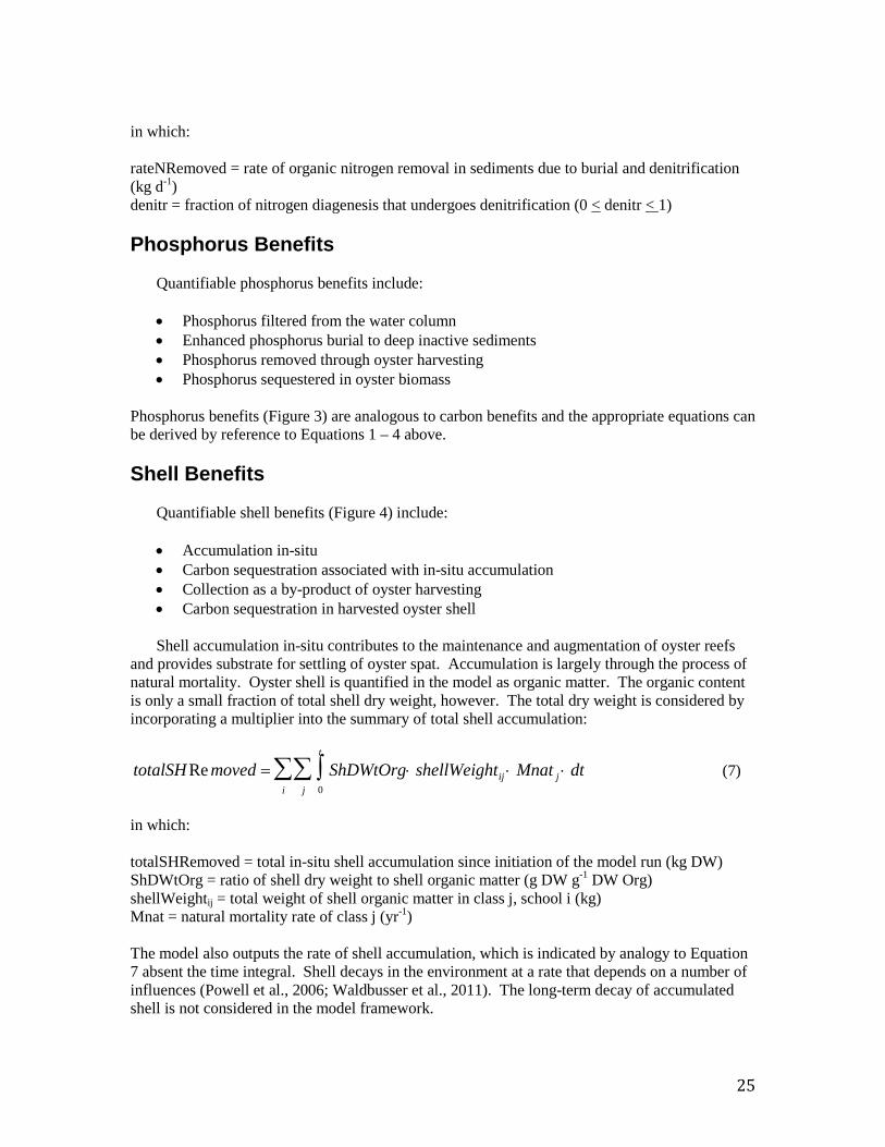
in which: rateNRemoved = rate of organic nitrogen removal in sediments due to burial and denitrification (kg d-1) denitr = fraction of nitrogen diagenesis that undergoes denitrification (0 < denitr < 1) Phosphorus Benefits

Quantifiable phosphorus benefits include:

• Phosphorus filtered from the water column • Enhanced phosphorus burial to deep inactive sediments • Phosphorus removed through oyster harvesting • Phosphorus sequestered in oyster biomass

Phosphorus benefits (Figure 3) are analogous to carbon benefits and the appropriate equations can be derived by reference to Equations 1 – 4 above. Shell Benefits

Quantifiable shell benefits (Figure 4) include:

• Accumulation in-situ • Carbon sequestration associated with in-situ accumulation • Collection as a by-product of oyster harvesting • Carbon sequestration in harvested oyster shell

Shell accumulation in-situ contributes to the maintenance and augmentation of oyster reefs

and provides substrate for settling of oyster spat. Accumulation is largely through the process of natural mortality. Oyster shell is quantified in the model as organic matter. The organic content is only a small fraction of total shell dry weight, however. The total dry weight is considered by incorporating a multiplier into the summary of total shell accumulation:

totalSH Re moved = ShDWtOrg⋅ shellWeightij ⋅ Mnat j ⋅ dt0

t

∫j

∑i

∑ (7)

in which: totalSHRemoved = total in-situ shell accumulation since initiation of the model run (kg DW) ShDWtOrg = ratio of shell dry weight to shell organic matter (g DW g-1 DW Org) shellWeightij = total weight of shell organic matter in class j, school i (kg) Mnat = natural mortality rate of class j (yr-1) The model also outputs the rate of shell accumulation, which is indicated by analogy to Equation 7 absent the time integral. Shell decays in the environment at a rate that depends on a number of influences (Powell et al., 2006; Waldbusser et al., 2011). The long-term decay of accumulated shell is not considered in the model framework.

25

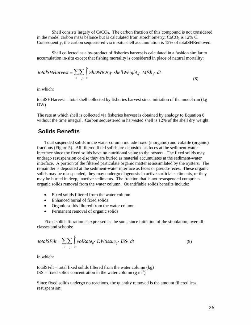
Shell consists largely of CaCO3. The carbon fraction of this compound is not considered in the model carbon mass balance but is calculated from stoichiometry; CaCO3 is 12% C. Consequently, the carbon sequestered via in-situ shell accumulation is 12% of totalSHRemoved. Shell collected as a by-product of fisheries harvest is calculated in a fashion similar to accumulation in-situ except that fishing mortality is considered in place of natural mortality:

totalSHHarvest = ShDWtOrg⋅ shellWeightij ⋅ Mfsh j ⋅ dt0

t

∫j

∑i

∑ (8)

in which: totalSHHarvest = total shell collected by fisheries harvest since initiation of the model run (kg DW) The rate at which shell is collected via fisheries harvest is obtained by analogy to Equation 8 without the time integral. Carbon sequestered in harvested shell is 12% of the shell dry weight. Solids Benefits

Total suspended solids in the water column include fixed (inorganic) and volatile (organic) fractions (Figure 5). All filtered fixed solids are deposited as feces at the sediment-water interface since the fixed solids have no nutritional value to the oysters. The fixed solids may undergo resuspension or else they are buried as material accumulates at the sediment-water interface. A portion of the filtered particulate organic matter is assimilated by the oysters. The remainder is deposited at the sediment-water interface as feces or pseudo-feces. These organic solids may be resuspended, they may undergo diagenesis in active surficial sediments, or they may be buried in deep, inactive sediments. The fraction that is not resuspended comprises organic solids removal from the water column. Quantifiable solids benefits include:

• Fixed solids filtered from the water column • Enhanced burial of fixed solids • Organic solids filtered from the water column • Permanent removal of organic solids

Fixed solids filtration is expressed as the sum, since initiation of the simulation, over all

classes and schools:

totalSFilt = volRateij ⋅ DWtissueij ⋅ ISS⋅ dt0

t

∫j

∑i

∑ (9)

in which: totalSFilt = total fixed solids filtered from the water column (kg) ISS = fixed solids concentration in the water column (g m-3) Since fixed solids undergo no reactions, the quantity removed is the amount filtered less resuspension:

26

totalSRe moved = totalSFilt⋅ 1 − resusp( ) (10) in which: totalSRemoved = fixed solids permanently deposited in the bottom sediments (kg) Organic solids in the model framework include phytoplankton, zooplankton, and detritus and are quantified as carbon. The particulate organic carbon in each of these classes can be converted to volatile solids via the quantity DWtoC, which is the ratio of dry weight to organic carbon in volatile solids. Consequently, the quantity of volatile solids filtered from the water column is a multiplier of the quantity of particulate carbon filtered from the water column:

totalVSSFilt = DWtoC⋅ totalCFilt (11) in which: totalVSSFilt = total volatile solids filtered from the water column (kg).

Volatile solids are removed from the system at the same rate at which particulate organic carbon is deposited in the active sediments. Once material is deposited, the influence of diagenesis is irrelevant since respired carbon does not return in particulate form. By incorporating DWtoC and eliminating respiration, Equation 2 yields:

rateVSSRe moved = DWtoC⋅ rateCRecycle + rateCNatMort + rateCSpawn[ ]⋅FLPOC + FRPOC[ ]⋅ 1 − resusp( ) (12)

in which: rateVSSRemoved = rate at which volatile solids are removed from the water column (kg d-1)

The rate of volatile solids removal is summed over all classes and schools and integrated over time to give totalVSSRemoved (kg), the total volatile solids removed via deposition since initiation of the model run. References Ferreira, J., Sequeira, A., Hawkins, A., Newton, A., Nickell, T., Pastres, R., Forte, J., Bodoy, A.,

and Bricker, S. (2009). “Analysis of coastal and offshore aquaculture: Application of the FARM model to multiple systems and shellfish species,” Aquaculture, 289(1-2,3), 32-41.

Grabowski, J., and Peterson, C. (2007) “Restoring oyster reefs to recover ecosystem services,”

Theoretical Ecology Series 4, 281-298. Jenkins, M., and Kemp, W. (1984). “The coupling of nitrification and denitrification in two

estuarine sediments,” Limnology and Oceanography 29(3), 609-619. Kellogg, L., Cornwell, J., Owens, M., and Paynter, K. (2013). “Denitrification and nutrient

assimilation on a restored oyster reef,” Marine Ecology Progress Series 480, 1-19.

27

Newell, R. (2004). “Ecosystem services of natural and cultivated populations of suspension-

feeding bivalve mollusks: A review,” Journal of Shellfish Research 23(1), 51-61. Powell, E., Kraeuter, J., and Ashton-Alcox, K. (2006). “How long does oyster shell last on an

oyster reef?,” Estuarine, Coastal and Shelf Science 69(3-4), 532-542. Waldbusser, G., Steenson, R., and Green, M. (2011). “Oyster shell dissolution rates in estuarine

waters: Effects of pH and shell legacy,” Journal of Shellfish Research 30(3), 659-669.

Figure 1. The model carbon cycle including oysters. The quantifiable benefits include carbon removal via fisheries harvest and carbon removal via burial to deep, inactive sediments.

28

Figure 2. The model nitrogen cycle including oysters. The quantifiable benefits include nitrogen removal via fisheries harvest, nitrogen removal through burial to deep, inactive sediments, and nitrogen removal via denitrification.

29

Figure 3. The model phosphorus cycle including oysters. The primary benefits include phosphorus removal via fisheries harvest and phosphorus removal via burial to deep, inactive sediments.

30

Figure 4. A simplified representation of processes affecting oyster shell in the water column and bottom sediments. Quantifiable benefits include shell accumulation in-situ and shell collected as a by-product of fisheries harvest.

31

Figure 5. The modeled influence of oysters on fixed and volatile suspended solids. The primary benfits are burial of both forms to deep, inactive sediments.

32

5 Application to the Great Wicomico River

The bioenergetics model is parameterized and demonstrated through application to the Great Wicomico River, Virginia (Figure 1). The Great Wicomico, a tributary located on the western shore of Chesapeake Bay between the mouths of the Potomac and Rappahannock Rivers, is selected for two reasons. First, the system is the subject of multiple studies by the Corps of Engineers including several investigations related to this effort. Second, oyster dynamics in the system have been extensively studied and published (Southworth et al., 2010). The reported population dynamics provide an excellent data set for evaluating model parameters and demonstrating applicability. The Great Wicomico River The Great Wicomico extends roughly 20 km from the junction with Chesapeake Bay to the upstream limit of tidal influence. The geometry is convoluted and the shoreline is punctuated with numerous embayments and tributaries. Mean depth is 2.7 m, surface area is 25 km2, and tide range is 0.335 m. Computations from a watershed model (Shenk and Linker, 2013) indicate the average flow at the head of tide is 1 to 2 m3 s-1. During a typical 12-hour period, less than 105 m3 of runoff enters the system from the watershed. During the same interval, 8.4 x 106 m3 of water is exchanged with Chesapeake Bay through tidal action. Thus, tidal exchange is the primary transport process in the system despite the small tide range. Water temperature cycles from roughly 5 to 30 oC over the course of a year while salinity ranges from roughly 10 to 20 ppt. Oyster Population Dynamics Population trends in the Great Wicomico from 2000 through 2009 were examined in detail by Southworth et al. (2010). They examined seven public reefs that were separated by physical features into upstream and downstream populations. One overarching conclusion of their study was that high mortality from disease was balanced by episodic and extraordinary recruitment events. Data they reported that found use in model parameterization and validation included:

• Individual oyster biomass (dry tissue weight) • Oyster age vs. shell length • Standing stock (population and biomass) • Shell accretion rates • Age structure and age-specific mortality • Recruitment rates

Model Parameter Values The Tidal Prism Model The tidal prism model (Chapter 3) requires specification of three physical properties: volumetric runoff rate (Qin), tidal prism volume (Tp), and system volume (V). Runoff was obtained from the Chesapeake Bay Program Watershed Model (WSM, Shenk and Linker, 2013). Since the WSM application period did not correspond to the study interval, ten years of daily

33

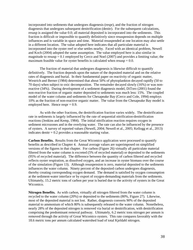
computed runoff (1991 – 2000) were summarized into long-term monthly values for use in the tidal prism representation. The monthly runoff varied from 0.45 m3 s-1 in June to 2.10 m3 s-1 in March. Volumes of the tidal prism (8.4 x 106 m3) and of the system at mean tide (67.5 x 106 m3) were obtained from a preceding model of the Great Wicomico (Kim et al., 2001). Loads and Boundary Conditions The tidal prism representation requires specification of concentrations in runoff and at the open mouth for each simulated substance (Table 3-1). Runoff concentrations were obtained from the WSM. The procedure for obtaining concentration followed the procedure for runoff volume; monthly means were determined from WSM output for the period 1991 – 2000. Concentrations at the mouth were obtained from a monitoring program conducted by the USEPA Chesapeake Bay Program (CBP, 2013). Samples for 2000 – 2009 were available at roughly monthly intervals at station CB5.4W (Figure 1). Linear interpolation was employed to estimate daily values between sampling events. Water temperature at the mouth cycles between 2 and 30 oC on an annual basis (Figure 2). Salinity at the mouth ranges from 9 to 21 ppt (Figure 3). Salinity fluctuations are irregular and influenced by freshwater pulses from the large watersheds in the upper Bay and Potomac River. Dissolved oxygen cycles between 6 and 14 g m-3 (Figure 4). The cycling corresponds to the annual cycling of temperature. Minimum DO concentration occurs during mid-summer when saturation concentration is least and temperature-driven respiration is high. Maximum DO concentration occurs in winter when saturation concentration is highest and temperature-driven respiration is low. The model calculates that temperature, salinity, and DO within the Great Wicomico are nearly identical to conditions outside the mouth. Model Application and Validation Temperature and Salinity The temperature computed by the tidal prism model was compared to reported temperature for the Great Wicomico (Figure 5). The model is in close agreement with the preponderance of reported values. The computed temperature falls short of the maxima (≅ 30 oC) reported for several years, however. In the present application, water temperature is determined solely by the temperature of the inflows at either end of the system. The excess of reported temperature over the boundary conditions likely represents atmospheric heat input, which can be considered in more advanced applications. The optimal temperature for filtration is specified in the model as 27 oC; filtration declines at temperature above and below this maximum. Consequently, the filtration rate at 30 oC is little different from the filtration rate at 25 oC. The respiration rate, however, increases with temperature throughout the temperature range so that computed respiration is less than it would be if the reported maximum temperatures were achieved in the model. The reported salinity is based on multiple sources including in-situ measurements at two locations and regression relationship to observations in the near-by York River. The tidal prism model well-reflects the in-situ observations (Figure 6). The model parameterization computes no effect of salinity on filtration unless salinity falls below 10 ppt. Both the observations and the model indicate salinity effects on oysters in this system are minimal.

34

Individual Oysters Southworth et al. (2010) provide observations of “age at length” for the Great Wicomico oyster population. Comparison to shell length computed by the model is excellent (Figure 7). Both observations and model indicate an oyster achieves shell length ≅ 20 mm three months after entering the population. An oyster four years of age achieves shell length ≅ 100 mm. The observed population-average individual dry tissue weight ranges from 0.1 to 0.7 g (Figure 8). The observations indicate increasing weight from 2002 through 2005 and from 2006 to 2009. The trend in weight reflects trends in population (Figure 9). Large recruitment events occurred in 2002 and 2006 resulting in a large population of young, small oysters. Subsequent mortality produced a population of older, larger oysters (Figure 10). The model reproduces the trends in individual weight as well as the preponderance of observed values. The computed individual weight is high from 2005 to 2006 when the population consists of relatively few, older individuals. Population and Biomass The observed and computed populations reflect the magnitude of recruitment events. Population peaks in 2002 and 2006 (Figure 9) reflect large recruitment events in the same years (Figure 11). Recruitment was modeled by introducing a “school” of oysters equivalent to the reported young-of-year on July 1 of each year. Specification of young-of-year is crucial to modeling the population in the Great Wicomico. Employment of an average recruitment rate, for example, results in a different and far less accurate picture of the population, especially in the years after 2006 (Figure 12). Total oyster biomass is the product of two quantities: population and individual size. The observed biomass is uniform for 2000 through 2005 and is matched in magnitude by the model (Figure 13). The observed biomass climbs steeply following the 2006 recruitment event and is two to three times the model value. Inspection of the computed population and individual size indicates the model shortfall is the result of a shortfall in population (Figure 9). Two sensitivity runs were conducted in an attempt to increase the population and, hence, the total oyster biomass. In the first run, annual mortality was reduced from the calibration value of 1.2 yr-1 to 0.77 yr-1. In the second run, recruitment rate was doubled. The increase in recruitment resulted in an excess population (Figure 14). Although the rate could be “tuned” to reproduce the observed population, comparison of computed and observed biomass with increased recruitment (Figure 15) suggests this path is not worthwhile. The increased number of small individuals does not produce a sufficiently large increase in biomass for the years subsequent to 2006. Reducing the mortality improves computed population and biomass in the years 2006 - 2010 at the expense of diminished model performance in the years 2000 to 2005 (note especially the computed biomass in the years 2003 to 2005, Figure 15). The calibration mortality value was based on the observation that “four-year olds were absent throughout the system in all years examined” (Southworth et al., 2010). An annual mortality rate of 1.2 yr-1 results in 99% mortality at the end of four years. The mortality rate 0.77 yr-1 is based on the report that the lifespan of Virginia oyster is 6 to 8 years (National Research Council, 2004). From the viewpoint of model-data agreement, the resolution of the dilemma is to use a higher mortality rate for the years 2000 to 2005 and a lower rate for the years 2006 to 2009 (Figures 16, 17). The lower value conflicts with the noted absence of four-year-old oysters, however. The uniform rate of 1.2 yr-1 is retained for the balance of the report but the reader is

35

advised that improved model-data agreement could be obtained through detailed parameter specification. Shell Accretion Computed shell accretion rates are “order of magnitude” correct but generally fall short of reported values (Figure 18). The computed shortfall reflects similar trends in computed and observed population but the magnitude of the disparity between computed and observed accretion warrants the consideration of additional factors. The reported rates are in L m-2 yr-1 while shell in the model is quantified on the basis of energy content. The model energy content is equated to dry weight organic matter through the parameter EPRD (Table 2-1) and subsequently converted to dry weight shell through parameter ShDWtOrg (Chapter 4). The reported rates are readily converted to total volume through multiplication of the rate per unit area by the reported areas of the oyster reefs. Subsequent conversion of volume to dry weight shell, for comparison with the model, is problematic, however. The procedure used here is to first convert volume to wet weight using the factor 1 L wet shell = 587.3 g (Mann et al., 2009). Wet weight is converted to dry weight by noting that shell is 1.9 to 5.0% water (Waldbusser et al., 2011). For practical purposes, the citation indicates wet weight and dry weight are equivalent. The shells employed by Waldbusser et al., however, were cleaned after shucking or else aged and weathered. Their reported value likely represents the water content of shell but not the wet weight of fresh shell with residual organic material attached. Conversion problems may also result from the use of a volume-to-wet-weight ratio based on fresh live oysters to convert the mixture of live oysters, aged shell, and fragments collect in-situ by Southworth et al. Consequently, we conclude the computed shell accretion rates are within the order of magnitude of observed rates but site-specific volume-to-weight conversions are necessary for more accurate quantification. Material Recycling The cycling of material from the water, through oysters, and back to the water or bottom sediments is of critical interest when considering the impact of oysters on water quality. The results of oyster activity are usually considered beneficial (e.g. removal of particulate material from water and deposition to bottom sediments) and are cited as justification for the restoration of oyster populations. Potential detrimental effects (e.g. oxygen consumption, nutrient release) have been occasionally cited, however. Cerco and Noel (2007) summarized observed values of key recycle rates and compared them to rates computed in a mass-balance oyster model applied to Chesapeake Bay. The observed rates included filtration, respiration, ammonium excretion, and carbon deposition. The rates for these processes computed in the present model are presented in Figures 19 – 22. The computed rates are influenced by two principal factors. The first is temperature; minimum values for all rates correspond to the interval of minimum water temperature. The second is population. Biomass-specific rates tend to be higher when the population consists of a large number of small individuals e.g. 2006. Specific rates tend to be lower when the population is dominated by larger, older individuals. Computed rates from this study are compared to observations in Table 1. This table also reports values from Cerco and Noel (2007) to provide comparison between the mass-balance and bioenergetics model approaches. The filtration rate for this study is comparable, although lower, than most reported values. The difference is attributed to temperature effects. Most reported values are for temperature greater than 20 oC while the value for this study is an average which incorporates the annual temperature cycle. We conclude the filtration rate in this study

36

agrees with reported values and with the original model from which it was derived. Examination of computed and observed respiration rates reinforces the impact of temperature on the comparisons. The average value computed by the present model agrees well with the annual average reported by Dame et al. (1992) but is less than reported values restricted to spring and summer. The ammonium excretion rates and carbon deposition rates from the present model are large compared to observations and to the previous model. The large values from the present model reflect differences in reported quantities. The model values are the total ammonium and carbon recycled through excretion (ammonium), feces and psuedofeces (carbon), and also mortality and spawning. The reported rates for ammonium represent excretion only while the reported carbon deposition values are for feces and pseudofeces. The values from the present model are, therefore, expected to exceed the values reported for processes that make up only a portion of the total recycled material. The model values are appropriate for mass-balance purposes although they do not compare perfectly with values based on recycling from live oysters only. Budgets and Benefits Nutrient and Solids Fluxes The quantification of oyster benefits amounts to a quantification of material fluxes, in particular the transfer of material from the water column to bottom sediments. Improved insight into these transfers comes from viewing first the material fluxes through the system from the watershed and out the mouth. The flux through the system consists of three components: load from the watershed, load on the incoming tidal prism and loss on the outgoing tidal prism. Each component is readily calculated via the mass-balance equation that describes the tidal prism approach (Equation 2, Chapter 3). The fluxes for total Kjeldahl Nitrogen (TKN), total phosphorus, and fixed solids are shown in Figures 23 – 25 respectively. We consider TKN here since it represents the nitrogen forms (ammonium plus organic nitrogen) that are influenced by oysters. Nitrate nitrogen can be a large fraction of total nitrogen load, especially for the watershed, but the nitrate is not influenced by oyster activity. The figures indicate the predominant nutrient and solids fluxes in the Wicomico are through the mouth. The quantities carried in and out on the tidal prism are two orders of magnitude greater than the load from the watershed. In the absence of any biological activity, we would expect the material flux on the outgoing tidal prism to exceed the flux on the incoming prism. The excess consists of the load from the watershed. Fluxes on the outgoing prism do, in fact, often exceed incoming fluxes, especially during colder portions of the year, when oyster activity is minimal, and during intervals of higher watershed loading. There are intervals, however, when the outgoing prism carries less material than the incoming prism. In these instances, the difference represents material retained in the Wicomico through oyster activity. At all times, however, the watershed loads and the accumulations due to oysters are vastly exceeded by the twice-daily tidal flows through the mouth of the embayment. Oyster Benefits

Calculation of oyster benefits requires the specification of several key parameters. These include the fraction of deposited material that is resuspended (resusp), the fraction of material

37

incorporated into sediments that undergoes diagenesis (respr), and the fraction of nitrogen diagenesis that undergoes subsequent denitrification (denitr). For the subsequent calculations, resusp is assigned the value 0.0; all material deposited is incorporated into the sediments. This fraction is difficult or impossible to quantify definitively since resuspension depends on multiple influences and is variable in space and time. Material resuspended at one location may also settle in a different location. The value adopted here indicates that all particulate material is incorporated into the oyster reef or else settles nearby. Faced with an identical problem, Newell and Koch (2004) adopted the same assumption. The value employed here is also similar in magnitude to resusp = 0.1 employed by Cerco and Noel (2007) and provides a limiting value; the maximum feasible value for oyster benefits is calculated when resusp = 0.0.

The fraction of material that undergoes diagenesis is likewise difficult to quantify

definitively. The fraction depends upon the nature of the deposited material and on the relative rates of diagenesis and burial. In their fundamental paper on reactivity of organic matter, Westrich and Berner (1984) determined that about 50% of phytoplankton decayed rapidly (50 to 70 days) when subject to oxic decomposition. The remainder decayed slowly (16%) or was non-reactive (34%). During development of a sediment diagenesis model, DiToro (2001) found the non-reactive fraction of organic matter deposited to sediments was much less: 15%. The coupled model of the water column and sediments for Chesapeake Bay (Cerco and Cole, 1994) employs 10% as the fraction of non-reactive organic matter. The value from the Chesapeake Bay model is employed here. Hence respr = 0.9.

As with the other fractions, the denitrification fraction varies widely. The denitrification

rate in sediments is largely influenced by the rate of sequential nitrification-denitrification reactions (Jenkins and Kemp, 1984). The initial nitrification reaction requires oxygen in sediment microzones and in the overlying water. The rate can also be influenced by the presence of oysters. A survey of reported values (Newell, 2004; Newell et al., 2005; Kellogg et al., 2013) indicates denitr = 0.2 provides a reasonable starting value. Carbon Benefits. Results from the Great Wicomico application were processed to quantify benefits as described in Chapter 4. Annual average values are superimposed on simplified versions of the figures in that chapter. For carbon (Figure 26) virtually all particulate material filtered from the water column is excreted (5% of recycled material) or deposited to the sediments (95% of recycled material). The difference between the quantity of carbon filtered and recycled reflects oyster respiration, as dissolved oxygen, and an increase in oyster biomass over the course of the simulation (Figure 13). Although resuspension is zero, material deposited to the sediments influences the water column. Ninety percent of the deposited carbon undergoes diagenesis, thereby creating corresponding oxygen demand. The demand is satisfied by oxygen consumption at the sediment-water interface or by export of oxygen-demanding materials from the sediments. Ultimately, 15.2 metric tons of carbon per year is buried due to the activity of oysters in the Great Wicomico. Nitrogen Benefits. As with carbon, virtually all nitrogen filtered from the water column is recycled to the water column (20%) or deposited to the sediments (80%, Figure 27). Likewise, most of the deposited material is not lost. Rather, diagenesis converts 90% of the deposited material to ammonium of which 80% is subsequently released to the water column. Nonetheless, nearly 28% of the deposited nitrogen is removed via burial or denitrification, with denitrification comprising the predominant removal pathway. Ultimately, 6.2 metric tons nitrogen per annum is removed through the activity of Great Wicomico oysters. This rate compares favorably with the 18.6 metric tons per annum calculated watershed load of total Kjeldahl nitrogen.

38

Phosphorus Benefits. Consistent with the other components of biomass, virtually all phosphorus filtered from the water column is recycled (20%) or deposited to the sediments (80%, Figure 28). The values adopted for the calculation indicate 90% of the deposited material undergoes diagenesis and is recycled to the water column. The remainder is buried. Ultimately, 0.2 metric tons phosphorus per annum is removed through the activity of oysters in the Great Wicomico. This rate is about 10% of the estimated total phosphorus loading from the watershed, 2.3 metric tons per annum. Solids Benefits. The oysters cannot retain fixed solids. Consequently, all filtered fixed solids must be deposited at the sediment-water interface (Figure 29). As a first approximation, we assume none of this material is resuspended and all is buried. In the absence of resuspension, all filtered organic solids are also permanently removed although the pathway is not as simple as for fixed solids. A large fraction of organic solids is composed of organic carbon. Here, in fact, we use a simple multiplier, DWtoOrgC, to quantify organic solids as a multiple of organic carbon. The processes that convert organic carbon to dissolved or gaseous forms reduce organic solids in proportionate amounts. Organic solids disappear when filtered particulate organic carbon is excreted in dissolved form. Likewise, organic solids deposited to the sediments disappear when respiration converts organic carbon to CO2. Consequently, the burial of organic solids is much less that the amount filtered although the amount filtered is the amount removed. Under the present assumptions, 822 metric tons fixed solids and 492 metric tons organic solids per annum are removed from the Great Wicomico water column through the activity of oysters. Shell Benefits. Natural oyster mortality contributes 108 tons DW shell to the Great Wicomico each year (Figure 30). We neglect the effects of decay, which impacts accumulation rather than deposition. Considering that shell is 12% carbon, 13 metric tons of carbon is deposited each year. This amount rivals the burial of organic carbon, 15.2 tons. The sources and forms of the carbon are different as is the environmental significance. The organic carbon originates as organic matter in the water column. Removal and subsequent burial removes potentially oxygen-demanding material from the water. The burial also contributes to sequestration of atmospheric carbon since a portion of the organic carbon originates through primary production of organic matter from CO2. The shell carbon originates as CO2 and is incorporated into shell through formation of CaCO3. The burial of shell contributes to carbon sequestration but the CO2 incorporated into shell has no alternative detrimental potential. Discussion We present here a basic approach to calculating oyster benefits. Numerous simplifications have been made to facilitate the calculation. We review in this section the costs and benefits of the simplifications and when more complex approaches might yield superior results.

We did not consider biogeochemical transformations in the water column. This simplification vastly eases the application of the bioenergetics model and allows the user to focus on oysters. The material fluxes attributable to oysters are isolated since these are the only biogeochemical fluxes calculated. This approach is most suitable when the concentrations of substances within a system are dominated by loads and boundary conditions rather than by transformations within the water column. In view of the volume of materials carried on the tidal prism, this approximation seems warranted for the Wicomico although proof requires calculation of the neglected transformations. The greatest loss in not considering the water column is the neglect of primary production of particulate carbon and associated transformation of dissolved

39

nutrients to particulate form. Absent the primary production of particulate carbon, the amount of carbon filtered by oysters and subsequently deposited to the bottom is potentially underestimated. Absent the transformation of dissolved nutrients into particulate form, the deposition of nitrogen and phosphorus may also be underestimated. The links to the CE-QUAL-ICM eutrophication model remain in the bioenergetics model code and ICM can be readily implemented. CE-QUAL-ICM has demonstrated capacity to calculate primary production (Cerco and Noel, 2004) and detailed capacity for calculating nutrient transformations (Cerco and Cole, 1994). The price for the implementation is in labor and complexity. We employ a single parameter, resusp, to quantify the fraction of deposited material that is subsequently resuspended by the actions of currents and waves. In fact, this fraction is virtually impossible to quantify precisely (Newell and Koch, 2004) and not readily addressed by more complex models that incorporate physical sediment transport processes. The fraction is variable in space and time, as are the currents and winds that drive resuspension. Studies indicate that waves and currents are themselves influenced by the presence of oyster reefs (Smith et al., 2009). Resuspension is also dependent on local bathymetry and bottom characteristics. The application of more advanced techniques is hampered by the difficulty and cost of relevant field measurements for parameterizing and verifying more advanced calculations. In view of these factors, the single parameter employed here presents a reasonable approach and more complex methods are not recommended. The prudent employer of this approach will, however, consider a range of potential resuspension fractions and report a range of potential benefits. The fraction of material that undergoes diagenesis requires lengthy and complex laboratory experiments to measure. The difficulty associated with measurement likely accounts for the paucity of observations. The predominant means of evaluating the fraction is through recursive parameter evaluation in coupled models of loading, water column processes, and sediment diagenesis. Two well-accepted studies that followed this procedure (DiToro, 2001; Cerco and Cole, 1994) evaluate the reactive fraction at 85% to 90% of the material deposited. These fractions are larger than the results obtained from one of the few detailed studies of organic matter reactivity (Westrich and Berner, 1984). In view of the extensive employment of the higher reactivity fractions, however, the employment of respr = 0.85 to 0.90 is recommended. As with resuspension and reactivity, the fraction of nitrogen diagenesis that undergoes denitrification is uncertain. Unlike resuspension and reactivity, denitrification is subject to measurement in specialized laboratories (Cornwell et al., 1999). Due to the variable rates of denitrification and the myriad factors that influence the process, exact specification of the fraction would require measurements at virtually every location where oysters contribute to the nitrogen budget. Oysters themselves influence the rate, positively or negatively. Enhanced nitrogen deposition enhances denitrification but associated oxygen consumption of freshly deposited organic matter can deplete the oxygen supply required for the first step of the nitrification-denitrification reactions (Newell, 2004). Consequently, potential restoration actions that will substantially change organic matter deposition will require prediction of dentrification under the proposed new conditions. These predictions could be made with a predictive diagenesis model (e.g. DiToro, 2001) with associated cost in labor and complexity. For most cases, the approach considered here is sufficient. As with resuspension, the prudent employer of this approach will consider a range of values in his estimates of denitrification. The calculated carbon benefits are based on watershed loads and tidal prism fluxes of particulate carbon only. As noted earlier, primary production of particles within the Wicomico is neglected. Thus the calculated values likely represent minimum values of carbon benefits contributed by oysters. The nitrogen benefits are also likely minimum values since particulate

40

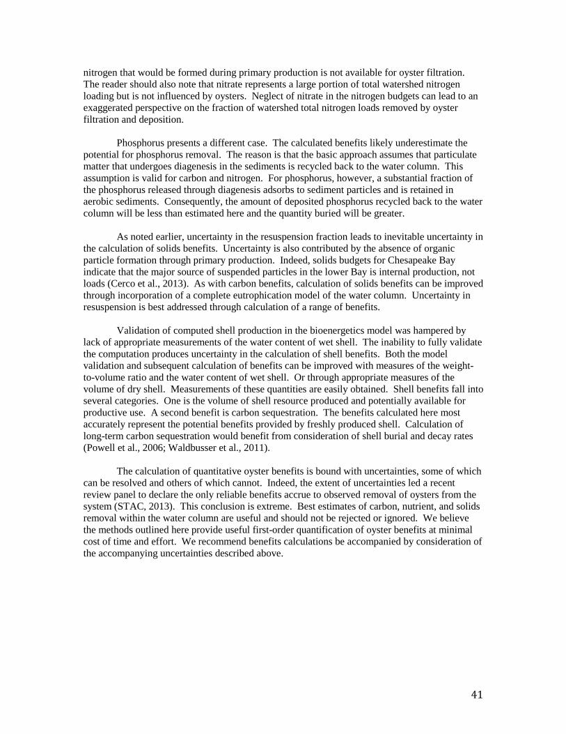
nitrogen that would be formed during primary production is not available for oyster filtration. The reader should also note that nitrate represents a large portion of total watershed nitrogen loading but is not influenced by oysters. Neglect of nitrate in the nitrogen budgets can lead to an exaggerated perspective on the fraction of watershed total nitrogen loads removed by oyster filtration and deposition. Phosphorus presents a different case. The calculated benefits likely underestimate the potential for phosphorus removal. The reason is that the basic approach assumes that particulate matter that undergoes diagenesis in the sediments is recycled back to the water column. This assumption is valid for carbon and nitrogen. For phosphorus, however, a substantial fraction of the phosphorus released through diagenesis adsorbs to sediment particles and is retained in aerobic sediments. Consequently, the amount of deposited phosphorus recycled back to the water column will be less than estimated here and the quantity buried will be greater. As noted earlier, uncertainty in the resuspension fraction leads to inevitable uncertainty in the calculation of solids benefits. Uncertainty is also contributed by the absence of organic particle formation through primary production. Indeed, solids budgets for Chesapeake Bay indicate that the major source of suspended particles in the lower Bay is internal production, not loads (Cerco et al., 2013). As with carbon benefits, calculation of solids benefits can be improved through incorporation of a complete eutrophication model of the water column. Uncertainty in resuspension is best addressed through calculation of a range of benefits.

Validation of computed shell production in the bioenergetics model was hampered by lack of appropriate measurements of the water content of wet shell. The inability to fully validate the computation produces uncertainty in the calculation of shell benefits. Both the model validation and subsequent calculation of benefits can be improved with measures of the weight-to-volume ratio and the water content of wet shell. Or through appropriate measures of the volume of dry shell. Measurements of these quantities are easily obtained. Shell benefits fall into several categories. One is the volume of shell resource produced and potentially available for productive use. A second benefit is carbon sequestration. The benefits calculated here most accurately represent the potential benefits provided by freshly produced shell. Calculation of long-term carbon sequestration would benefit from consideration of shell burial and decay rates (Powell et al., 2006; Waldbusser et al., 2011).

The calculation of quantitative oyster benefits is bound with uncertainties, some of which

can be resolved and others of which cannot. Indeed, the extent of uncertainties led a recent review panel to declare the only reliable benefits accrue to observed removal of oysters from the system (STAC, 2013). This conclusion is extreme. Best estimates of carbon, nutrient, and solids removal within the water column are useful and should not be rejected or ignored. We believe the methods outlined here provide useful first-order quantification of oyster benefits at minimal cost of time and effort. We recommend benefits calculations be accompanied by consideration of the accompanying uncertainties described above.

41

References Cerco, C., and Cole, T. (1994). “Three-dimensional eutrophication model of Chesapeake Bay,”

Technical Report EL-94-4, US Army Corps of engineer Waterways Experiment Station, Vicksburg MS.

Cerco, C., and Noel, M. (2004). “Process-based primary production modeling in Chesapeake

Bay,” Marine Ecology Progress Series, 282, 45-58. Cerco, C., and Noel, M. (2007). “Can oyster restoration reverse cultural eutrophication in

Chesapeake Bay?,” Estuaries and Coasts 30(2), 331-343. Cerco, C., Kim, S-C., and Noel, M. (2013). “Management modeling of suspended solids in the

Chesapeake Bay, USA,” Estuarine, Coastal and Shelf Science 116, 87-98. Chesapeake Bay Program. (2013). “Chesapeake Bay Program Data Hub,” US EPA Chesapeake

Bay Program, Annapolis MD (http://www.chesapeakebay.net/data). Cornwell, J., Kemp, W., and Kana, T. (1999). “Denitrification in coastal ecosystems: methods,

environmental controls, and ecosystem level controls, a review,” Aquatic Ecology 33, 41-54.

Dame, R., Spurrier, J., and Zingmark, R. (1992). “In situ metabolism of an oyster reef,” Journal

of Experimental Marine Biology and Ecology 164, 147-159. DiToro, D. (2001). Sediment Flux Modeling, John Wiley and Sons, New York. Jenkins, M., and Kemp, W. (1984). “The coupling of nitrification and denitrification in two

estuarine sediments,” Limnology and Oceanography 29(3), 609-619. Kellogg, M., Cornwell, J., Owens, M., and Paynter, K. (2013). “Denitrification and nutrient

assimilation on a restored oyster reef,” Marine Ecology Progress Series 480, 1-19. Kim, S-C., Wetzel, R., Haas, L., and Kuo, A. (2001). “Application of a watershed model

(BASINSIM) and a tidal prism model to the Great Wicomico River, Virginia,” Virginia Institute of Marine Science, Gloucester Point VA.

Mann, R., Southworth, M., Harding, J., and Wesson, J. (2009). “Population studies of the native

oysters, Crassostrea virginica (Gmelin), in the James River, Virginia, USA,” Journal of Shellfish Research 28, 193-220.

National Research Council. (2004). “Oyster biology,” Committee on Nonnative Oysters in

Chesapeake Bay, National Academies Press, Washington DC. Newell, R. (2004). “Ecosystem influences of natural and cultivated populations of suspension-

feeding bivalve molliscs: A review,” Journal of Shellfish Research 23(1), 51-61.

42

Newell, R., and Koch, E. (2004). “Modeling seagrass density and distribution in response to changes in turbidity stemming from bivalve filtration and seagrass sediment stabilization,” Estuaries 27(5), 793-806.

Newell, R., Fisher, T., Holyoke, R., and Cornwell, J. (2005). “Influence of eastern oysters on

nitrogen and phosphorus regeneration in the Chesapeake Bay, USA.” The comparative roles of suspension-feeders in ecosystems. R. Dame and S. Olenin eds., Springer, the Netherlands.

Powell, E., Kraeuter, J., and Ashton-Alcox, K. (2006). “How long does oyster shell last on an

oyster reef?,” Estuarine, Coastal and Shelf Science 69, 531-542. Shenk, G., and Linker, L. (2013). “Development and application of the 2010 Chesapeake TMDL

watershed model,” Journal of the American Water Resources Association, 49(5), 1042-1056.

Smith, K., North, E., Shi, F., Chen, S-N., Hood, R., Koch, E., and Newell, R. (2009). “Modeling

the effects of oyster reefs and breakwaters on seagrass growth,” Estuaries and Coasts 32(4), 748-757

Southworth, M., Harding, J., Wesson, J., and Mann, R. (2010). “Oyster (Crassostrea virginica,

Gmelin 1791) population dynamics on public reefs in the Great Wicomico River, Virginia, USA,” Journal of Shellfish Research 29(2), 271-290.

Scientific and Technical Advisory Commitee. (2013). “Evaluation of the use of shellfish as a

method of nutrient reduction in the Chesapeake Bay,” STAC Publication 13-005, Chesapeake Research Consortium, Edgewater MD. (http://www.chesapeake.org/pubs/307_Luckenbach2013.pdf)

Waldbusser, G., Steenson, R., and Green, M. (2011). “Oyster shell dissolution rates in estuarine

waters: Effects of pH and shell legacy,” Journal of Shellfish Research 30(3), 659-669. Westrich, J., and Berner, R. (1984). “The role of sedimentary organic matter in bacterial sulfate

reduction: The G model tested,” Limnology and Oceanography 29(2), 236-249.

43

Table 1 Modeled and Observed Biomass-Specific Oyster Effects Property Rate Source Comments Filtration rate, m3 g-1 oyster C d-1

0.17 This study Ten-year average

0.24 Cerco and Noel (2007)

Summer average

0.22 Jordan (1987)

Mean value, T > 20 oC

0.26 Newell and Koch (2004)

Average of measures at 20 and 25 oC

0.027 to 0.33 Epifanio and Ewart (1977)

For algal suspensions > 1 g C m-3

0.27 Riisgard (1988)

Calculated for a 2.1 g DW oyster at 27 to 29 oC

Respiration rate, g DO g-1 oyster C d-1

0.013 This study Ten-year average

0.04 Cerco and Noel (2007)

Summer average

0.03 to 0.06 Boucher and Boucher-Rodini (1988)

Spring and summer rates

0.017 Dame et al. (1992)

Annual average

0.02 Dame (1972) 1 g DW oyster at 20 to 30 oC Ammonium excretion, mg N g-1 oyster C d-1

6.13 This study Ten-year average

1.43 Cerco and Noel (2007)

Summer Average

< 0.1 Hammen et al. (1966)

Ammonium plus urea

2.8 to 3.88 Boucher and Boucher-Rodini (1988)

Spring and summer rates, includes urea

0.8 Srna and Baggaley (1976)

1 g DW oyster at 20 oC

4.8 to 7.9 Magni et al (2000)

Ruditapes and musculista

Carbon deposition, g C g-1 oyster C d-1

0.223 This study Ten-year average

0.088 Cerco and Noel (2007)

Summer average

0.099 Jordan (1987)

Mean value, T > 20 oC

0.03 Haven and Morales-Alamo (1966)

0.002 to 0.012

Tenore and Dunstan (1973)

Depends on C concentration, range is 0.1 to 0.7 g C m-3

44

Figure 5-1. The Great Wicomico River. Sample station CB5.4W is indicated.

45

Figure 5-2. Temperature observed at the mouth of the Great Wicomico and computed in the interior.

46

Figure 5-3. Salinity observed at the mouth of the Great Wicomico and computed in the interior.

47

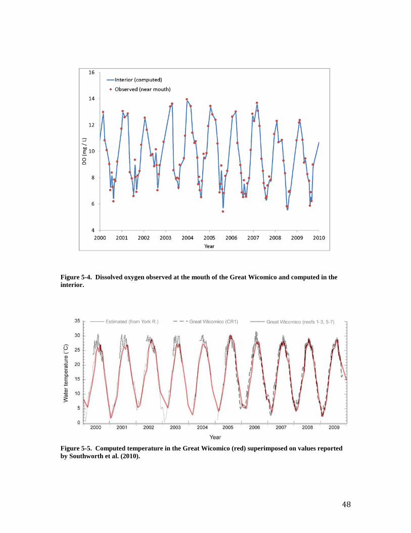
Figure 5-4. Dissolved oxygen observed at the mouth of the Great Wicomico and computed in the interior.

Figure 5-5. Computed temperature in the Great Wicomico (red) superimposed on values reported by Southworth et al. (2010).

48

Figure 5-6. Computed salinity in the Great Wicomico (red) superimposed on values reported by Southworth et al. (2010).

Figure 5-7. Computed and observed (Southworth et al., 2010) “age at length” relationships.

49

Figure 5-8. Computed and observed (Southworth et al., 2010) population-average individual dry tissue weight.

50

Figure 5-9. Computed and observed (Southworth et al., 2010) oyster population.

51

Figure 5-10. Computed and observed (Southworth et al., 2010) average age of oyster population.

52

Figure 5-11. Observed (Southworth et al., 2010) “young-of-year.”

53

Figure 5-12. Sensitivity of computed population to recruitment rate. Two computations are shown, one based on observed recruitment in individual years, the other based on recruitment rate averaged over all years.

54

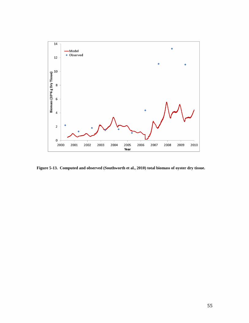
Figure 5-13. Computed and observed (Southworth et al., 2010) total biomass of oyster dry tissue.

55

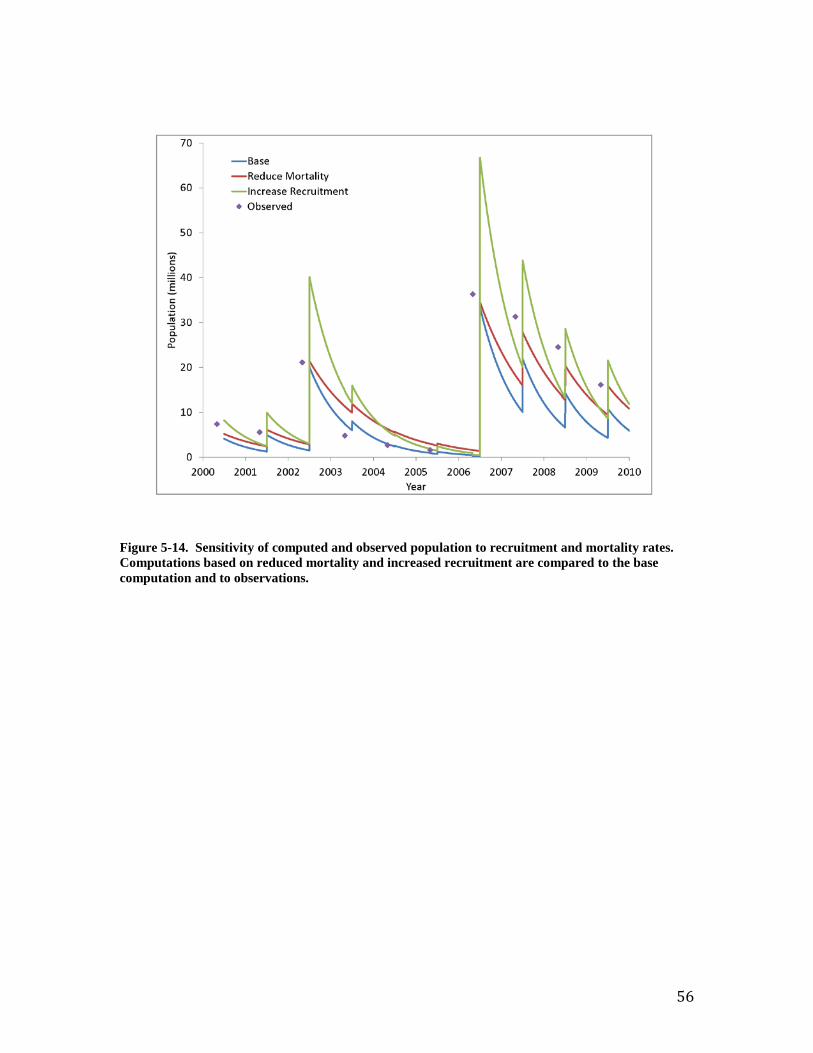
Figure 5-14. Sensitivity of computed and observed population to recruitment and mortality rates. Computations based on reduced mortality and increased recruitment are compared to the base computation and to observations.

56

Figure 5-15 Sensitivity of computed total biomass to recruitment and mortality rates. Computations based on reduced mortality and increased recruitment are compared to the base computation and to observations.

57

Figure 5-16. Population computed on the basis of two mortality rates, 1.2 yr-1 for 2000 – 2005 and 0.77 yr-1 for 2006 – 2010.

58

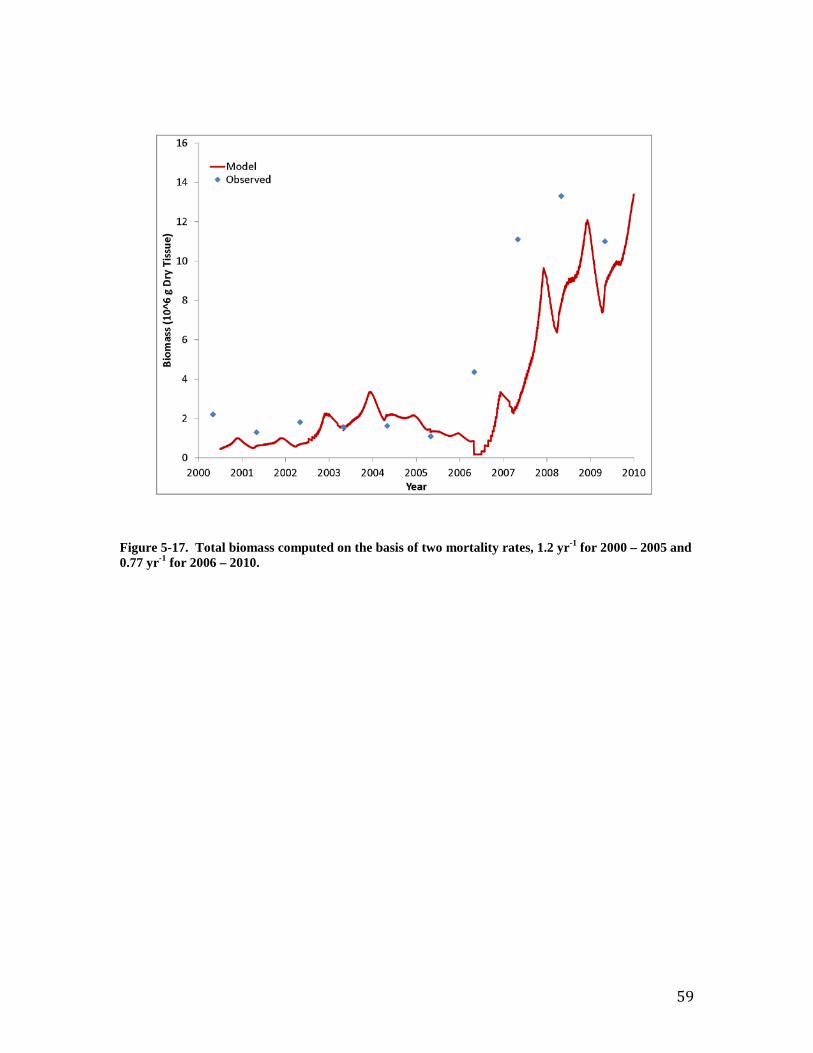
Figure 5-17. Total biomass computed on the basis of two mortality rates, 1.2 yr-1 for 2000 – 2005 and 0.77 yr-1 for 2006 – 2010.

59

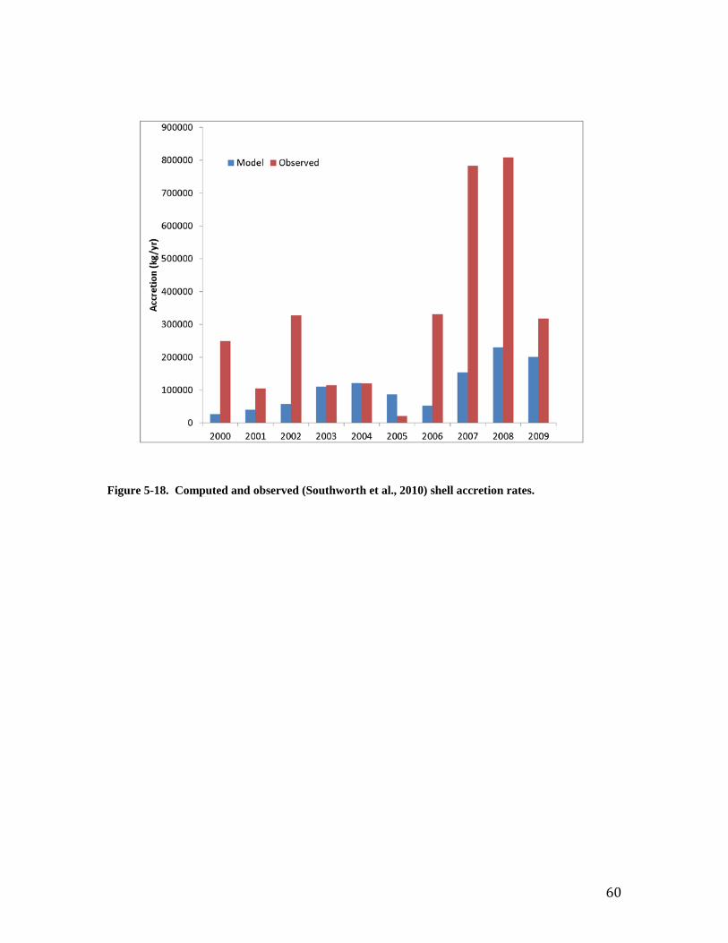
Figure 5-18. Computed and observed (Southworth et al., 2010) shell accretion rates.

60

Figure 5-19. Computed specific filtration rate, averaged over all individuals.

61

Figure 5-20. Computed specific respiration rate, averaged over all individuals.

62

Figure 5-21. Computed specific ammonium excretion rate, averaged over all individuals.

63

Figure 5-22. Computed specific carbon deposition rate, averaged over all individuals.

64

Figure 5-23. Computed TKN fluxes through the Great Wicomico.

65

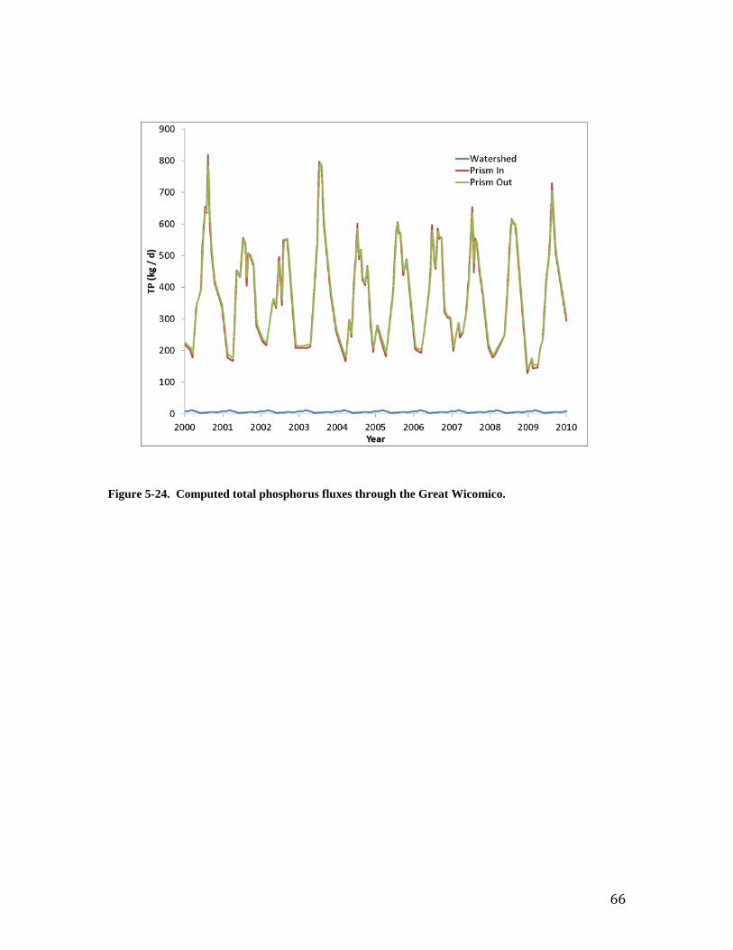
Figure 5-24. Computed total phosphorus fluxes through the Great Wicomico.

66

Figure 5-25. Computed fixed (inorganic) solids fluxes through the Great Wicomico.

67

Figure 5-26. Computed carbon fluxes and benefits in the Great Wicomico. All values are annual averages in metric tons.

68

Figure 5-27. Computed nitrogen fluxes and benefits in the Great Wicomico. All values are annual averages in metric tons.

69

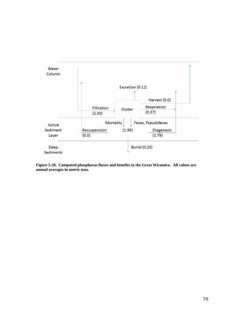
Figure 5-28. Computed phosphorus fluxes and benefits in the Great Wicomico. All values are annual averages in metric tons.

70

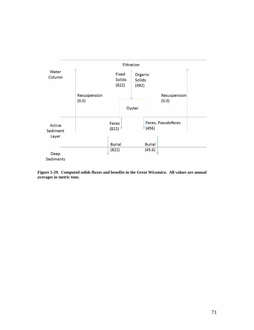
Figure 5-29. Computed solids fluxes and benefits in the Great Wicomico. All values are annual averages in metric tons.

71

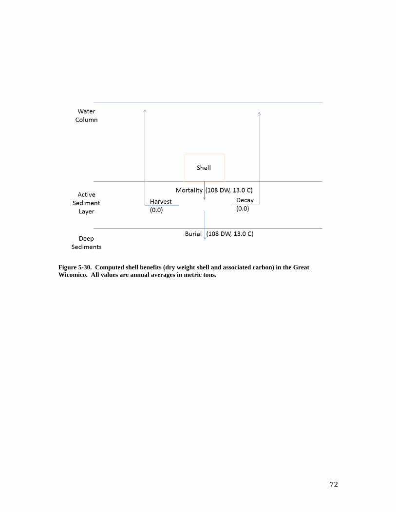
Figure 5-30. Computed shell benefits (dry weight shell and associated carbon) in the Great Wicomico. All values are annual averages in metric tons.

72

6 Summary and Conclusions Bivalve Bioenergetics Model The model considers two basic properties of a bivalve population: number of individuals and individual size. Energy (quantified in joules) is the basic model “currency.” The model formulation originated in the Wisconsin Fish Model (Hanson et al., 1997) and was adapted for a model of Atlantic menhaden in Chesapeake Bay (Dalyander and Cerco, 2010). Subsequent investigations explored the potential for extension of the menhaden bioenergetics model to Virginia oysters (Crassostrea virginica) and culminated in the present report. The model heritage also extends to a carbon-based mass-balance oyster model that was employed to investigate the impacts of a ten-fold increase in Chesapeake Bay oyster population (Cerco and Noel, 2007). Parameters quantified during that study were employed to the greatest extent possible in this investigation. The model considers three stores of energy within the individual oyster: shell, soft tissue, and reproductive material. The oysters filter overlying water continuously. When the quantity of particulate matter filtered from the water column exceeds the amount the oyster can ingest, the excess is rejected as pseudofeces. The remainder is consumed. A portion of consumption is ejected as feces and excretion. The remainder goes into production of one or more of the energy stores. Soft tissue is lost through respiration, at a rate determined by individual characteristics and by properties of the environment. Two forms of respiration are considered. Active respiration is a constant fraction of the energy expended in feeding. Basal metabolism proceeds at a rate independent of activity. Reproductive material is lost through spawning, which occurs when sufficient reproductive energy is accumulated and when conditions in the environment are appropriate. The bioenergetics model offers several advances over the preceding mass-balance model. The most significant is the representation of the three energy stores (shell, soft tissue, reproductive material). The preceding model considered only soft tissue. Significant quantities of energy (and equivalent organic matter) are in the two additional stores. Consequently, the present model is a more realistic representation of energy flow in bivalves. From a practical viewpoint, the present formulation considers the sequestration of carbon and nutrients in organic matter associated with shell. The transformation and fate of these elements can be significant when considering potential oyster benefits. Consideration of the number of individuals provides a much more realistic representation of population dynamics and population biomass than a mass-balance model. This advantage is countered, however, by the need for realistic estimates of annual recruitment. The use of long-term average values for recruitment produces a significantly different picture of oyster biomass than the use of annually varying values.

In summary, the detailed representations of individual and population processes in the present model are worthwhile developments. It is not clear, however, that energy needs to be the currency of the model. The use of energy is a hindrance when the bioenergetics model is coupled to a mass-balance model of a physical system. Conversion factors and multiple back-and-forth conversions between energy and mass are required. A carbon or dry-weight based oyster model, with the same processes and components as the present model, would serve as well as an

73

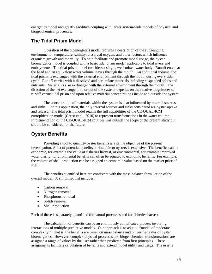
energetics model and greatly facilitate coupling with larger system-wide models of physical and biogeochemical processes. The Tidal Prism Model

Operation of the bioenergetics model requires a description of the surrounding environment – temperature, salinity, dissolved oxygen, and other factors which influence organism growth and mortality. To both facilitate and promote model usage, the oyster bioenergetics model is coupled with a basic tidal prism model applicable to tidal rivers and embayments. The tidal prism model considers a single, well-mixed water body. Runoff enters at the head and an equivalent water volume leaves through the mouth. An additional volume, the tidal prism, is exchanged with the external environment through the mouth during every tidal cycle. Runoff carries with it dissolved and particulate materials including suspended solids and nutrients. Material is also exchanged with the external environment through the mouth. The direction of the net exchange, into or out of the system, depends on the relative magnitudes of runoff versus tidal prism and upon relative material concentrations inside and outside the system.

The concentration of materials within the system is also influenced by internal sources

and sinks. For this application, the only internal sources and sinks considered are oyster uptake and release. The tidal prism model retains the full capabilities of the CE-QUAL-ICM eutrophication model (Cerco et al., 2010) to represent transformations in the water column. Implementation of the CE-QUAL-ICM routines was outside the scope of the present study but should be considered for the future. Oyster Benefits Providing a tool to quantify oyster benefits is a prime objective of the present investigation. A list of potential benefits attributable to oysters is extensive. The benefits can be economic, for example the value of fisheries harvest, or environmental, for example improved water clarity. Environmental benefits can often be equated to economic benefits. For example, the volume of shell production can be assigned an economic value based on the market price of shell. The benefits quantified here are consistent with the mass-balance formulation of the overall model. A simplified list includes:

• Carbon removal • Nitrogen removal • Phosphorus removal • Solids removal • Shell production

Each of these is separately quantified for natural processes and for fisheries harvest. The calculation of benefits can be an enormously complicated process involving interactions of multiple predictive models. Our approach is to adopt a “model of moderate complexity.” That is, the benefits are based on mass balance and on verified rates of oyster bioenergetics. However, complex physical processes and biogeochemical transformations are assigned a range of values by the user rather than predicted from first principles. These assignments facilitate calculation of benefits and extend model utility and usage. The user is

74

cautioned, however, that calculation of a range of benefits based on a reasonable range of parameter values is preferred to calculation of an exact benefit based on a single parameter assignment. The Great Wicomico River

The model is demonstrated through application to the Great Wicomico River, Virginia, 2000 - 2009. The Great Wicomico is selected for two reasons. First, the system is the subject of multiple studies by the Corps of Engineers including several investigations related to this effort. Second, oyster dynamics in the system have been extensively studied and published (Southworth et al., 2010). The reported population dynamics provide an excellent data set for evaluating model parameters and demonstrating applicability. Data that found use in model parameterization and validation included:

• Individual oyster biomass (dry tissue weight) • Oyster age vs. shell length • Standing stock (population and biomass) • Shell accretion rates • Age structure and age-specific mortality • Recruitment rates

The Great Wicomico was represented using the tidal prism approach and loads and boundary conditions adopted from various Chesapeake Bay Program data sets (Shenk and Linker, 2013; Chesapeake Bay Program, 2013). The approach provided good representation of temperature, salinity, and dissolved oxygen, the primary physical factors that drive oyster bioenergetics. Model representations of particulate carbon and nutrients would be improved, however, through implementation of the CE-QUAL-ICM kinetics in the water column. The bioenergetics model provided excellent representation of individual oyster size, of population number, and of average individual age. Representation of total population biomass fell short of observations at times, apparently due to the assignment of a constant mortality rate. Improved computations were possible by utilizing two mortality rates in the course of the ten-year simulation. An overarching conclusion from the application was that representation of the detailed data set required corresponding detailed information on recruitment, mortality, and other factors. The oyster benefits module was demonstrated through application to the Great Wicomico. We concluded that 164 metric tons of carbon per annum is filtered from the water column by oysters and 15.2 tons is buried to deep inactive sediments. An additional 13 metric tons of carbon is buried in the form of shell. Oysters filter 28 metric tons nitrogen per annum from the Great Wicomico water column. Most is recycled but, ultimately, 6.2 metric tons nitrogen per annum is removed through denitrification and burial of oyster deposits. This nitrogen rate compares favorably with the 18.6 metric tons per annum calculated watershed load of total Kjeldahl nitrogen. Oysters filter 2.5 metric tons phosphorus per annum of which 0.2 tons is permanently removed by burial to deep inactive sediments. The loss of phosphorus is proportionately less than nitrogen because no process analogous to denitrification exists for phosphorus. Oysters are calculated to remove 822 metric tons fixed solids and 492 metric tons organic solids per annum. Our estimates are the maximum potential amounts absent resuspension.

75

The calculation of quantitative oyster benefits is bound with uncertainties, some of which can be resolved and others of which cannot. We believe the methods described here provide useful first-order quantification of oyster benefits at minimal cost of time and effort. We recommend benefits calculations be accompanied by consideration of the accompanying uncertainties described in Chapter 5 of the text. Next Steps The bioenergetics model has been formulated, programmed, applied, and compared to observations. There are numerous next steps to facilitate model application, to further validate the model, and to extend the applicability. Graphical User Interface. The model presently operates on a linux workstation. Input files are prepared by the user, using a text editor. Output files are processed in MATLAB and graphed using a variety of user-provided applications. Transfer of the model to a PC Windows operating system is underway as is the completion of a Graphical User Interface to facilitate preparation of input and output files. Additional Validation for Virginia Oysters. The model has been extensively compared to multiple observed properties of Virginia oysters in the Great Wicomico River. Additional validation of the model parameter set against observations in other systems is desirable. Aquaculture. The model application is to a natural population at home in an oyster reef. In the Chesapeake Bay, especially, oyster cultivation is rapidly increasing and a range of benefits is touted to result (e.g. Bricker et al., 2014). Aquaculture facilities are different than natural reefs, however, and model modifications are required to represent various aquaculture practices. Model verification at one or more aquaculture facilities is also recommended. Implement with Full Eutrophication Model. The bioenergetics model is coupled to a complete model of eutrophication processes in estuarine waters. The eutrophication routines were not implemented, however, for the Great Wicomico. Since phytoplankton production was not computed, the filtration of carbon by oysters was potentially underestimated, as was the filtration of particulate nutrients incorporated into plankton biomass. As a consequence, carbon and nutrient benefits (removal) were potentially underestimated as well. Application of the complete model capabilities to compute biogeochemical transformation in the water column is recommended, followed by comparison to results from the simplified version employed here. Incorporate into Alternate System Models. A re-examination of the potential benefits of oyster restoration and of aquaculture is planned for the 2017 re-evaluation of the Chesapeake Bay Total Maximum Daily Loads. Following the recommended additional validation for Virginia oysters (above), the present formulation could be adopted for Chesapeake Bay. Extension to Other Bivalves. The bioenergetics formulation should be applicable to a range of filter-feeding bivalves. This includes other species of oysters, other desirable bivalves, as well as nuisance organisms such as Zebra mussels. The extension to other species requires model parameterization and validation with appropriate data sets.

76

References Bricker, S., Rice, K., and Bricker, O. (2014). “From headwaters to coast: Influence of human

activities on water quality of the Potomac River Estuary,” Aquatic Geochemistry 20, 291-323.

Cerco, C., and Noel, M. (2007). “Can oyster restoration reverse cultural eutrophication in

Chesapeake Bay?,” Estuaries and Coasts 30(2), 331-343. Cerco, C., Kim, S.-C., and Noel, M. (2010). “The 2010 Chesapeake Bay eutrophication model,”

Report to the US Environmental Protection Agency Chesapeake Bay Program and to the US Army Engineer District Baltimore. (available at http://www.chesapeakebay.net/publications/title/the_2010_chesapeake_bay_eutrophication_model1)

Chesapeake Bay Program. (2013). “Chesapeake Bay Program Data Hub,” US EPA Chesapeake

Bay Program, Annapolis MD (http://www.chesapeakebay.net/data). Dalyander, P., and Cerco, C. (2010). “Integration of a fish bioenergetics model into a spatially-

explicit water quality model: Application to menhaden in Chesapeake Bay,” Ecological Modelling 221, 1922-1933.

Hanson, P., Johnson, T., Schindler, D., and Kitchell, J. (1997). “Fish bioenergetics 3.0,” WISCU-

T-97-001, University of Wisconsin Sea Grant Institute, Madison WI. Shenk, G., and Linker, L. (2013). “Development and application of the 2010 Chesapeake TMDL

watershed model,” Journal of the American Water Resources Association, 49(5), 1042-1056.

Southworth, M., Harding, J., Wesson, J., and Mann, R. (2010). “Oyster (Crassostrea virginica,

Gmelin 1791) population dynamics on public reefs in the Great Wicomico River, Virginia, USA,” Journal of Shellfish Research 29(2), 271-290.

77