Institutionen f�or systemteknikDepartment of Electrical Engineering

Examensarbete

Brake Calculation Software for Commercial Vehicles

Tor-�Ake Fransson

LiTH-ISY-EX-1983

1998-12-01

TEKNISKA H�OGSKOLAN

LINK�OPINGS UNIVERSITET

Department of Electrical Engineering Link�opings tekniska h�ogskolaLink�opings universitet Institutionen f�or systemteknikS-581 83 Link�oping, Sweden 581 83 Link�oping

Brake Calculation Software for

Commercial Vehicles

M. Sc. Thesis for Vehicular Systemsat Link�oping Institute of Technologyperformed at Scania CV, S�odert�alje

by

Tor-�Ake Fransson

Reg nr: LiTH-ISY-EX-1983

Supervisor: Nils-Gunnar V�agstedt, Scania CV

Examiner: Lars Nielsen , Vehicular Systems LiTH

Link�oping, 2nd December 1998.

Avdelning, InstitutionDivision, Department

Datum:Date:

Spr�akLanguage

2 Svenska/Swedish

2 Engelska/English

2

RapporttypReport category

2 Licentiatavhandling

2 Examensarbete

2 C-uppsats

2 D-uppsats

2 �Ovrig rapport

2

URL f�or elektronisk version

ISBN

ISRN

Serietitel och serienummerTitle of series, numbering

ISSN

Titel:

Title:

F�orfattare:

Author:

Sammanfattning

Abstract

Nyckelord

Keywords

Department of Electrical Engineering

Division of Vehicular Systems

LiTH-ISY-EX-1983

http://www.vehicular.isy.liu.se/

1998-12-01

Bromsber�akningsprogram f�or tunga fordonBrake Calculation Software for Commercial Vehicles

Tor-�Ake Fransson

��

To ensure that a commercial vehicle has su�cient braking performance, prop-erties as friction utilization, braking rate and braking distances are examined.Calculating the brake performance is, though not matematically di�cult, verytime consuming. Using modular concepts of vehicle design, a vast number of con-�gurations regarding dimensions, weight and braking equipment adds further tothe time and energy laid on brake related calculations.

The natural solution to the problem is to seek aid from computers. However,computerized brake calculations, in order to be e�cient, needs highly special-ized software. Presented, is a program explicitly designed to calculate brakingperformance for commercial vehicles.

Design emphasis is laid upon user frendliness, and modularity providing foreasy upgrading of the program for dealing with future products.

The modular vehicle model used, tailored to computer aided braking perfor-mance calculation, is presented also.

Commercial vehicle, Brake performance calculation, Software

Abstract i

Abstract

To ensure that a commercial vehicle has su�cient braking performance, propertiesas friction utilization, braking rate and braking distances are examined. Calcu-lating the brake performance is, though not matematically di�cult, very timeconsuming. Using modular concepts of vehicle design, a vast number of con�gu-rations regarding dimensions, weight and braking equipment adds further to thetime and energy laid on brake related calculations.

The natural solution to the problem is to seek aid from computers. However,computerized brake calculations, in order to be e�cient, needs highly specializedsoftware. Presented, is a program explicitly designed to calculate braking perfor-mance for commercial vehicles.

Design emphasis is laid upon user frendliness, and modularity providing foreasy upgrading of the program for dealing with future products.

The modular vehicle model used, tailored to computer aided braking perfor-mance calculation, is presented also.

Keywords: Commercial vehicle, Brake performance calculation, Software

Preface iii

Preface

This thesis is the �nal report to a Masters degree in Mechanical Engineering atthe Link�oping Institute of Technology (Link�opings Tekniska H�ogskola, LiTH). Thework was conducted at Scania CV AB in S�odert�alje between June and November1998.

Acknowledgments

I would like to thank all the people at Scania CV and LiTH who have helped methrough this work.

Special thanks to Nils-Gunnar V�agstedt for guidance around the obstacles thatappeared during the work and valuable opinions in general.

Thanks also to Peter Engelke for proof reading and valuable feedback, and toall the people at the Brake, Suspension & General Vehicle Systems Departmentfor their support.

Contents

1 Introduction 1

1.1 Background . . . . . . . . . . . . . . . . . . . . . . . . . . . . . . . 1

1.2 Purpose . . . . . . . . . . . . . . . . . . . . . . . . . . . . . . . . . 2

1.3 Literature Survey . . . . . . . . . . . . . . . . . . . . . . . . . . . . 2

1.4 Disposition . . . . . . . . . . . . . . . . . . . . . . . . . . . . . . . 2

2 Problem Description 3

2.1 Brake Calculations . . . . . . . . . . . . . . . . . . . . . . . . . . . 3

2.2 Software Requirements . . . . . . . . . . . . . . . . . . . . . . . . . 4

3 Brake Calculation Software 7

3.1 The WBrake Program . . . . . . . . . . . . . . . . . . . . . . . . . 7

3.1.1 Design Philosophy . . . . . . . . . . . . . . . . . . . . . . . 7

3.1.2 Graphical User Interface . . . . . . . . . . . . . . . . . . . 8

3.1.3 Component Database . . . . . . . . . . . . . . . . . . . . . 9

3.1.4 Output . . . . . . . . . . . . . . . . . . . . . . . . . . . . . 10

3.1.5 Development Tools . . . . . . . . . . . . . . . . . . . . . . . 10

3.2 Use Example . . . . . . . . . . . . . . . . . . . . . . . . . . . . . . 11

4 Model and Calculation Methods 15

4.1 Vehicle and Brake System Model . . . . . . . . . . . . . . . . . . . 15

4.1.1 Vehicle . . . . . . . . . . . . . . . . . . . . . . . . . . . . . 16

4.1.2 Bogie . . . . . . . . . . . . . . . . . . . . . . . . . . . . . . 17

4.1.3 Axle . . . . . . . . . . . . . . . . . . . . . . . . . . . . . . . 19

4.1.4 Brake . . . . . . . . . . . . . . . . . . . . . . . . . . . . . . 19

4.1.5 Tire . . . . . . . . . . . . . . . . . . . . . . . . . . . . . . . 21

4.1.6 Brake Cylinder . . . . . . . . . . . . . . . . . . . . . . . . . 21

4.1.7 Load Sensing Valve . . . . . . . . . . . . . . . . . . . . . . 22

4.1.8 Putting it Together . . . . . . . . . . . . . . . . . . . . . . . 23

4.2 Calculation Objectives . . . . . . . . . . . . . . . . . . . . . . . . 24

4.2.1 Braking Rate . . . . . . . . . . . . . . . . . . . . . . . . . . 24

4.2.2 Friction Utilization . . . . . . . . . . . . . . . . . . . . . . 26

v

vi CONTENTS

5 Discussion and Future Work 295.1 Database Re�nement . . . . . . . . . . . . . . . . . . . . . . . . . . 295.2 User Feedback . . . . . . . . . . . . . . . . . . . . . . . . . . . . . 295.3 Model Veri�cation . . . . . . . . . . . . . . . . . . . . . . . . . . . 30

Appendices 32

A Model Component Interface A

B Development Tools B

C Pneumatic Brake System C

D Regulations D

E Sample Output E

F LSV Model Comparison F

Nomenclature

SymbolsD Distance [m]F Force [N ]L Load [N ]M Moment [Nm]H Height [m]W Weight [kg]l Length [m]g Gravity constant 9.82[m=s2]� Mechanical e�ciency [-]P Point -p Pressure [bar]C Constant -

IndicesF FrontR RearFjR Front OR Rearn Normal (force)b Brake (force)eff E�ective

Chapter 1

Introduction

This chapter describes the background and the purpose of this thesis work. Adescription of the disposition of this report is included to help the reader in navi-gating this document.

1.1 Background

Brake calculations are performed to determine stopping distances, braking rate andfriction utilization for a vehicle. These properties are needed for determination ofwhat braking system components, in terms of brake cylinders, brake levers andload sensing valves the vehicle should be equipped with, and to show that a vehicleof a certain con�guration can meet requirements imposed by law.

At Scania, module concepts of design o�er a high level of freedom for thecustomer to specify the overall con�guration of the vehicle when ordering. Thisresults in manufacturing a wide variety of vehicle speci�cations, from two to �veaxles, with a number of di�erent axle distances. Other properties a�ecting brakeperformance is the customers choice of tires, ground clearance and inter-axle loaddistribution. Additionally, there are also di�erences in legal requirements on brakesbetween di�erent parts of the world.

Whenever a new vehicle con�guration or model is introduced, a brake calcu-lation must be performed. In earlier days, engineers at Scania performed thesecalculations by hand, and later with the aid of computers.

The software tools in use today are custom-made, small programs and spread-sheet macros, written by consultants, and in many cases by the engineers them-selves. There is no uniformity in the di�erent tools, and calculation methods areoften obscure to everyone but the tool designer. Often, this is inadequate, andthe calculation has to be performed in a semi-manual way, or by combining anexisting tool with own assumptions. This make brake calculations consume a lotof e�ort and time, in addition to increasing the hazard of miscalculation

1

2 CHAPTER 1. INTRODUCTION

1.2 Purpose

The purpose of this thesis work is to develop a user-friendly and powerful toolfor calculating the impact on braking properties from a vehicles braking system,collecting the theories and methods into one program, with a consistent user in-terface.

1.3 Literature Survey

To get an understanding of commercial vehicles braking, a brief literature surveywas performed at the Scania library. Older manually performed braking calcula-tions were examined for algorithms and formulas to use in the program.

1.4 Disposition

To aid in reading this report, a short description of each chapter is provided,presenting the thread leading from one chapter to the next.

Chapter 2: Problem Description gives a speci�c description of the problem,as introduced in Chapter 1, in terms of calculation di�culties and the requirementsfor a tool used in these calculations.

Chapter 3: Brake Calculation Software presents the chosen solution, for theproblem de�ned in Chapter 2. Thoughts behind the design, as well as tools used inthe development process are discussed. The way calculated results are presentedto the user is also discussed here. Finally, an example of how the program is tobe used is provided.

Note that this section is not intended to serve as a user manual.

Chapter 4: Model and Calculation Methods describes the vehicle modelused in the program introduced in Chapter 3, gives a description of how the partsinteract during calculation of di�erent properties, and shows calculation algorithm,using the model.

Chapter 5: Discussion and Future Work The resulting program, calculationresults, users opinions and acceptance of the program is discussed. Included aresuggestions where to emphasize future development, plus some possible extensionsof the program.

Chapter 2

Problem Description

2.1 Brake Calculations

Calculations on properties of the brakes of a vehicle are not theoretically di�cultto accomplish, providing that you have a proper calculation basis. Propertiessuch as braking distances, braking ratio and distribution of braking e�ort amonga vehicles axles can easily, though time-consuming, be calculated by hand, usingcarefully balanced approximations.

The reason for interest in the braking properties varies. A commercial vehiclesbrake performance is of course always vital, but it is especially important whena vehicle manufacturer needs to show that his product ful�lls the requirementsimposed by laws and regulations.

Considering the fact that Scania sells vehicles in numerous countries, withdi�erent regulations and demands are put on the product, in combination withthe fact that the vehicles are sold in a wide variety of con�gurations, it's easy torealize that the calculations are numerous.

The properties of special interest here are the braking rate and the frictionutilization (see Section 4.2). Occasions for examining these can be:

I When certifying new vehicle types

I When the marketing department is submitting an o�er

I Introducing a vehicle on a new market

I Specializing a vehicle for a certain task

I Impact study on new developments

The ordering instance of a brake calculation might not have all the parameterson a vehicle. The basis for the calculation must therefor introduce a number ofapproximations, weighings and quali�ed guesses of vehicle parameters. It is vital

3

4 CHAPTER 2. PROBLEM DESCRIPTION

Figure 2.1: Eight-wheeled vehicle with two front axles

to understand that reasonable results can be achieved anyway, while the accuracyof the results is a matter of discussion.

Another reason for simplifying the calculation basis is reducing the informationquantity that goes into a calculation, in order to minimize the total time from brakecalculation order to actual result. Reusing vehicle parameters, by saving them foruse at other calculations, where large con�guration parts are the same allows forsomewhat more re�ned calculations, without having to input a large amount ofvehicle data.

At the same time, a mathematical model must not be too simple. If oneregards the vehicle in Figure 2.1, it becomes obvious that a sti� body model isnot adequate for calculating e.g the reaction forces from ground on wheels. Theimportance grows with the impact of brake pitching on the ground reactions.

Summarized, this will form the requirements set upon a tool to use for brakecalculations.

2.2 Software Requirements

From previous attempts of making a specialized application for brake calculationssome conclusions can be drawn:

User friendliness is important. A lot of time can be wasted if the functionof some part of the program is misunderstood. Also, credibility of the calculationcan get questioned if an incorrect calculation is presented to e.g certi�cation au-thorities.

Prepare for easy upgrading. Documentation of the inner structure of theprogram provides for code reusage, and is a requirement for adding functionalityto an existing program.

Stability. Few things are as annoying as having to redo work just becausethe tool crashed. If it, for some reason, is impossible for a program to continueexecuting, it should at least be possible to save partial work.

2.2. SOFTWARE REQUIREMENTS 5

Platform independence. Since computer evolution is rapid, software turnsunusable simply because the machine or operating system it executes on is re-placed. Preparing the source code for compilation on other architectures is a goodstrategic move.

Krister Lindstr�om, a former employee at the TCTSB department and extensiveuser of a brake calculation program developed for MS-DOS(R) in 1990-1993 drafteda set of requirements based on his experience:

I A new program should be written in a stable and well-known language

I Simple and nice-looking user interface

I Clear and self-instructing

I Nice-looking and legible result printouts

I Printout results in both tabular and plot form

I Should be able to calculate using di�erent types of brakes

I Should be able to calculate for various national regulations

Lindstr�om also emphasizes modularity and upgradability.Further demands regarding the vehicle component parameters storing were also

presented by Nils-Gunnar V�agstedt:

Data consistency. The parameters for a vehicle component should be con-tinuously updated to avoid deviation from reality. Some form of fully or partlyautomated updating of parameters regarding e.g geometry of a bogie, to avoiderroneous results caused by use of inactual data.

Automated calculations. Using already-present vehicle data e.g in an ex-isting database, the calculation should be performable without having to separatelyspecify these parameters through the user interface of the program.

Chapter 3

Brake Calculation Software

3.1 The WBrake Program

This section describes an implementation of software aided brake calculations, thewbrake program. It is an application built to serve one purpose: brake calculationsfor commercial vehicles.

3.1.1 Design Philosophy

The internal structure of the program was built with two major concerns: mod-ularity and object orientation. Figure 3.1 shows the main modules, events and

GUI

Calc.

Vehicle

Kernel

Calc.

Database

EventsData

Figure 3.1: Application internal structure

data ows within the program. Events trigger actions in a module, e.g causing

7

8 CHAPTER 3. BRAKE CALCULATION SOFTWARE

a window to redraw, or a recalculation of internal parameters. Only a modulesending events to another need knowledge of internal structures of the receiver.Data ows (e.g objects and parameters) are pulled by the receiver. In theory, amodule could be changed completely, without having to change a module fetchingdata from it, as long as the data interface is kept the same. Using this schemeprovides possibility to replace (some) modules without having to change others.

The modules in the WBrake program are:

Graphical User Interface. As Figure 3.1 imposes, it can be replaced with-out having to change the implementation of the vehicle model and parts database.

Kernel. This is where the work is done in the program. It controls calcu-lation through the vehicle model and forms user output shown in the GUI and onpaper printouts. This module can be changed without updating the vehicle modeland parts database.

Vehicle Model. This module implements the mathematical vehicle modeldescribed in 4.1.

Components Database. This module stores vehicle components and brakeregulation data. See Section 3.1.3.

3.1.2 Graphical User Interface

The GUI is what the user of the application sees, and through which the userinteracts with the program. Guidelines when designing this user interface were:

I Use computer memory rather than human. Present all information that isneeded simultaneously in one view, to avoid tiring the users mind.

I Place similar functions together. If functions, used for the same thing arescattered over a wide area, the user wastes time and energy refocusing at-tention.

I Use pictures and symbols wisely. A graphic can help the user get an overviewof a substantial amount of data, but unnecessary use of symbols instead oftext can cause great confusion.

I Input in any order. The basis for the calculation might come with vehicledata in any order. For �rst time users, 'any order' input can be confusing,but to slightly experienced users, �xed order input is an annoying constraint.

The user interface was built with the wxWindows library (see Appendix B and[4]).

3.1. THE WBRAKE PROGRAM 9

Figure 3.2: Graphical User Interface (Main window)

The main window of the user interface (see Fig 3.2) contains controls for alluser con�gureable parts of the vehicle model and calculation. These are: bogiecontrols (labelled 4), brake equipment controls (labelled 2), a display showing theoverall con�guration (labelled 1) and a calculation result display (labelled 3).

3.1.3 Component Database

The component database stores information about vehicle components, as e.g thegeometry for a bogie, in accordance with the requirements set in Section 2.1.

The database is loaded by the program upon startup, so de�ning the vehiclemodel properties is really done by selecting components, using the GUI controls.As a result of this, calculating the brake properties for a vehicle, though the modelcontains hundreds of parameters, is done in a matter of seconds.

Storing paramaters in a database also minimizes the hazard of miscalculationbecause of faulty parameters, providing, of course, that the parameters stored fora component is correct.

Ideal would be, if there was a company database, containing all the compo-nents available for building vehicles, to extract data from. That way, the dataused for calculations would always be consistent with reality. No such databaseis available at Scania at this point, however, but the modularity of the wbrakeprogram provides for an implementation change of the components database toinclude such functionality.

The storage method chosen here is plain text �les, with a program moduleacting as a database manager (DBMS), receiving queries and returning componentdata. This scheme opens the possibility to incorporate a commercial standarddatabase, should it be needed for performance reasons. The reason for not doingso in the current implementation is simplicity, plus avoiding platform dependance,

10 CHAPTER 3. BRAKE CALCULATION SOFTWARE

which would be the case with a commercial database where source code usually isnot supplied.

Figure 3.3: GUI for de�ning load sensing valve characteristics

De�ning components for storage in the database is done either by simply addingthe parameters to the plain text �les, or in the case of more obscure components,through the graphical user interface, as shown in Figure 3.3.

3.1.4 Output

Results from the calculations with the WBrake program are ground reaction forcesand brake forces for each axle. These results are processed in various ways topresent the sought properties, �rst in preview plots, see Figure 3.2, and then on atwo-page printout, see Figure 3.4.

On the result printouts, the vehicle is described in forms of overall con�guration(labelled 1 in Figure 3.4), and information about braking equipment (labelled 2and 3). The processed calculation results are presented as graphs (labelled 4) andtables (labelled 5 and 6).

The tables (5 and 6) provide essentially the same information as the plots (4),so the page layout is chosen so that all information is available on page 1, andprinting page 2 is optional.

Authentic printouts are provided in Appendix E.

3.1.5 Development Tools

The tools used for the development of the WBrake program had to ful�ll veryspeci�c requirements about cross-platform compability and performance.

The C++ compiler had to be available on all the intended platforms1and beable to generate working, debuggable programs from ANSI C++ code. The only

1Linux, IRIX, AIX and Win32

3.2. USE EXAMPLE 11

Figure 3.4: Result printouts

viable choice was the EGCS compiler from the GNU project (see [5]), which workson virtually all computer operating systems used today.

Likewise, the GUI library had to be multi-platform capable, though in theory,the GUI could be separately written for each platform. It also had to have properC++ bindings, to avoid having to revert to C2, for certain parts of the program.

The source code editor of choice was GNU Emacs, with an exception for theIRIX platform, where XEmacs was used. Emacs has the basic features of a sourcecode editor, e.g syntax indentation and highlighting, and it is, similar to EGCS,available on all the used platforms.

Debugging the program was done using the GNU debugger, gdb, which workedon all platforms except AIX, for unknown reasons. If development, other thancompiling already debugged source code, is to be performed on AIX, the debuggingissue has to be resolved.

A complete list of the used development software, including version informa-tion, is available in Appendix B.

3.2 Use Example

Using the program to calculate brake properties for a vehicle is done in a fewsimple steps, once the components used are stored in the database.

2C is the de-facto standard binding for GUI toolkits

12 CHAPTER 3. BRAKE CALCULATION SOFTWARE

Front Bogie Rear BogieUnladen Load [ton] 5.0 4.9Laden Load [ton] 8.2 16.0

Bogie Type Single axle Leaf spring suspended balance bogie

Axle 1 Axle 2 Axle 3Tire 14.00 - 20 14.00 - 20 14.00 - 20Brake drum brake drum brake drum brake

Brake Cylinder Size 30 20 16

Load Sensing Valve noneAxle Distance [mm] 4000

Trailer Valve Pred. [bar] 0.2

Unladen LadenCG Height [mm] 1100 1550

Table 3.1: Example Vehicle Con�guration

For �nding out the trailer compability (braking rate characteristics) for a ve-hicle with con�guration as table 3.1, the walkthrough looks like:

1. Create the vehicle by selecting 'new->truck' from the �le menu. The GUIshows a tractor (Figure 3.5) without wheels.

2. Select type of bogie for front and rear, respectively. Controls for per-axlecon�guration appears.

3. Fill in the values for CG height and axle distance.

4. For each axle of the vehicle, select tire, brake and chamber (Figure 3.6).

5. Select load sensing valve type and trailer valve predominance value.

6. Select regulations, and preview case (corridor position).

7. Fill out the loads for front and rear bogie. The program calculates thebraking rate and shows preview plots (Figure 3.7).

8. To get a paper hardcopy of the results, select 'print' from the �le menu. Aprint preview of page 1 is shown in Figure 3.8.

Conforming to the guidelines set in 3.1.2, step 3 to 7, above, can be performed inany order. The paper printout from step 8 is provided in appendix E.

3.2. USE EXAMPLE 13

Figure 3.5: Main window after creating new vehicle

Figure 3.6: Main window while selecting brake equipment

Figure 3.7: Main window when calculation is complete

Figure 3.8: Print preview window

Chapter 4

Model and Calculation

Methods

4.1 Vehicle and Brake System Model

This section describes a mathematical model of a vehicle, tailored to the speci�ccalculation objectives used in the program (see Section 4.2). Mathematical cor-rectness of the model, and adherence to 'the reality', is constrained, either bythe need to ful�ll algorithms de�ned in braking regulations, or by the strive forimplementation simplicity.

Since most equations used are linear, and many of the input values are some-what arbitrary, the accuracy of the results would not bene�t from a complex model,either. Instead, reasonable approximations are made where possible. Where atScania accepted algorithms exist, those have been used, even if their accuracy maydeviate somewhat from the model's general level.

The model is also created under the assumption that iteration is preferred overother mathematical solving techniques. The reason for this is that it is meant tobe easy to transform into C++ program code. While most desktop computers hascomputing power enough to iterate a formula several thousand times in fractionsof a second, a programmer needs several hours to implement any kind of 'smart'solving routine.

To provide for modularity, an object oriented approach is used throughoutthe model. Model parts are generalized as far as possible to form objects withconsistent interfaces.

A prerequisite for this is that model components need no knowledge of theintrinsics of components attached to it, they can only observe their behavior informs of outputs. This is also known as a 'black box' view. A component usinganother, typically, supplies inputs, e.g for a brake using a brake chamber, thecontrol pressure, and observes and uses the output, in this case a force. Figure 4.1shows the dependency tree for the whole vehicle model.

15

16 CHAPTER 4. MODEL AND CALCULATION METHODS

TyreBrake

Chamber

Axle (1) Axle (2) Axle (3)

Bogie (R)Bogie (F)

Regulations

LSV

Vehicle

Figure 4.1: Vehicle Model Components (tree view)

4.1.1 Vehicle

The vehicle model, preferably a tractor or truck, contains four or more wheels,certain dimensions and a mass. Since the concept of time is not at all used inany of the calculation objectives, there is no need for moments of inertia or otherdynamic properties.

It is also assumed that de ection of parts other than suspension is not of greatimportance for the results. Hence, the model does not rely upon information aboutthe physical structure of the vehicle it is modeling.

Consequently, the model part referred to as the 'Vehicle' is, from the programspoint of view, a 'black box' into which is put a weight, distributed over two suspen-sion points (bogies), a distance between these suspension points 1at rest, a centerof gravity height, and an air pressure, which represents the control pressure fromthe foot valve (see Appendix C).

The output consists of a retardation value (actually the ratio between brakingforce and weight) plus, for each axle on the vehicle, a ratio between the brake forceand the normal force, the adhesion utilization (see Section 4.2.2).

Transferring the inputs to outputs is done using two Bogie components. Eachof them are given a control pressure, which it transforms to a brake force. Thisinformation, along with the one supplied, is used to decide the resulting loaddistribution through equations 4.1 - 4.2. For symbols, see Figure 4.2.

1This property is given as an axle distance, de�ned as the distance between the frontmost axle

of the vehicle, and the �rst driven axle in the rear bogie.

4.1. VEHICLE AND BRAKE SYSTEM MODEL 17

LR �DA � Fb �HCG = 0 (4.1)

LR + LF �W � g = 0 (4.2)

If the vehicle is equipped with a load sensing valve (see Section 4.1.7), thecontrol pressure given to the rear bogie depends on the load distributed to it,which calls for iteration, since the brake force, in fact, becomes dependant of theretardation.

As a response to the loads, the bogie components also react with a de ection,from which the pitching angle of the vehicle is derived, through eqn. 4.3. Theneed for this is explained in section 4.1.2.

Fb1

Bogie

LF

DF DR

Bogie

CGH

L R

DA

Fb2

Fb

Figure 4.2: Vehicle - Bogie interaction

� = arcsin

�DF �DR

DA

�(4.3)

Regulations (see Appendix D) state how the center of gravity height shouldbe approximated. In general, the exact height of CG is not known, and oftennot derivable from supplied data either. This is unfortunate, since the impact onweight distribution calculation is directly proportional, as can be seen in eqn. 4.1.

The suspension point distance (axle distance when dealing with two-axle ve-hicles) in eqn. 4.1 is also a�ected by the output of the bogies. It is important tounderstand that this change does not come from any de ection of the vehicle. Itis simply a way to accommodate for the fact that the bogie can create a pitchingmoment, as well as a normal force.

A summary of inputs and outputs for this component is given in Appendix A.

4.1.2 Bogie

A bogie in its usual meaning, is a constellation of two or more axles mountedclose to eachother on a vehicle, more or less acting as a unit. In some cases amechanism for balancing load, on uneven surfaces, between the axles is present.This is usually a mechanical link system for leaf spring suspended bogies, or abellow pressure transfer device, of some sort, for air suspended bogies.

18 CHAPTER 4. MODEL AND CALCULATION METHODS

This makes the bogie the far most complex part of the vehicle model. It consistsof one to three axles, together with a set of functions to translate a load, a pitchangle and an air pressure, to forces and de ections that apply to the vehicle as awhole, and to forces that apply to each axle. To do this, it needs to be able to makequali�ed predictions about things like e.g spring constants for the suspension.

AxleAxle

PA

Fn Fb Fn Fb

FnM = 0

Figure 4.3: Bogie - Axle interaction

Given an air pressure, the bogie calculates the total braking force from itsaxles by summarizing their brake forces, respectively, and passes this value to thevehicle it is attached to. Calculated is also the normal force for each axle, withrespect to the bogie geometry, the pitching angle and the total load. The point ofattachment, (PAin Figure 4.2) which is used to calculate the dynamic axle distance(see Section 4.1.1) is the point in the bogie, around which the moment from normalforces is equal to zero.

FB1FB1

FB1

FB1

PA

DPA

l1 l2l3 l4

h1 h2 h3 h4

d2

Figure 4.4: Example bogie.

Exemplifying an air suspended two-axle bogie with direct pressure transfer,and bellows of equal size, as shown in Fig. 4.4, this model renders equations 4.4to 4.6 for the forces transfered to the vehicle, and eqn. 4.7 for the de ection.

FN1l1

l1 + l2+ FB1

h1

l1 + l2= FN2

l3l3 + l4

+ FB2h3

l3 + l4(4.4)

FN1 + FN2 = L � g (4.5)

DPA =FN2 � d2

FN1 + FN2(4.6)

4.1. VEHICLE AND BRAKE SYSTEM MODEL 19

DF jB = CB

l1l1+l2

+ l3l3+l4

2�

0@ FN1�l1+FB1�h1

l1+l2+ FN2�l3+FB2�h3

l3+l4

Lrest � g ��

l12(l1+l2)

+ l32(l3+l4)

� � 1

1A (4.7)

DPAis the distance from the �rst axle in the bogie to the point of attachmenton the vehicle. CB approximates the air bellow spring constant. Note that thereal spring constant for any air suspension is dependant on Lrest, the load at rest,because it e�ectively decides the air pressure in the bellow.

The di�erence in bogie behavior needs equations corresponding to eqn. 4.4- 4.7 to be set up for each bogie type, and ultimately coded in C++. That isnot ideal, but generalizing all bogie types to a �xed set of equations is virtuallyimpossible with the chosen approach.

A summary of all component inputs and outputs can be seen in Appendix A.

4.1.3 Axle

An axle is simply a sti� rod, laterally connecting two wheels. It can also providehousing for transmission, and/or steering, but that is of very little interest in thiscase.

The axles role in the vehicle model is merely to work as an attachment pointfor brakes and tires. The control pressure given to it by the bogie is passed onto the brake attached, and the resulting brake moment is divided by the dynamicrolling radius of the tire, thus giving a brake force, which is passed back to thebogie.

4.1.4 Brake

Using friction, a mechanical brake transfers energy in the form of motion intoenergy in the form of heat. Typically a pad is pressed against a rotating discor drum, creating a braking moment. The size of this braking moment can becalculated, with knowledge of how force (input) is transfered to the brake pad.

The brake cylinder force acts on a lever, which turns a cam, pressing the padagainst the rotating disc or drum. This is true for both the disc brake in Fig. 4.5,and the drum brake (see schematic in Fig. 4.6).

Equations 4.8 - 4.9 show how this model component transfers chamber force(Fcyl) to braking moment. Note that the 'servo factor', C in Eqn. 4.8 is 0.8 fora disc brake (roughly the number of pads times the friction coe�cient), while itis 1.9 for a drum brake, because of the self-amplifying geometry (the leading shoegets pressed towards the drum).

Mb =Mcam � C � Reff � �

Rcam

(4.8)

Mcam = llever � (Fcyl � Fthr) (4.9)

20 CHAPTER 4. MODEL AND CALCULATION METHODS

Figure 4.5: Disc brake with brake cylinder

FLever

Cam

Reff

Shoe

Figure 4.6: Drum brake schematic

4.1. VEHICLE AND BRAKE SYSTEM MODEL 21

Since the pads (disc brake) and shoes (drum brake) are springloaded, a thresh-old force is subtracted from the cylinder force. This threshold force is dependanton the brakes con�guration, and is given to the model component as a constant.

A summary of inputs and outputs of this component is provided in AppendixA.

4.1.5 Tire

The tire creates friction against the ground for braking, acceleration and corneringof the vehicle. It also de ects under load and provides for a somewhat smootherride.

From the WBrake model's point of view, however, it is only treated as a leverfrom the brake center to the ground, transferring braking moment to a force brak-ing the vehicle. The only important property is consequently its dynamic rollingradius, or the distance from its center to the ground, mounted on a vehicle.

4.1.6 Brake Cylinder

A brake cylinder contains a chamber, transforming air pressure into force. Itconsists of a spring-loaded diaphragm inside a cylinder, to which a pushrod isattached. The chamber is mounted near the brake, and actuates its force on alever mounted on the brake. See Figure 4.7 and schematic in Figure 4.8.

Figure 4.7: Brake cylinder �tted on vehicle (drum brake)

The mathematical model of this component is very simple. Air pressure (input)transforms to a force (output) through Eqn. 4.10.

F = C � Pm � Fthr (4.10)

The chamber diaphragm, on which the air pressure is applied is springloaded,which gives a threshold force, Fthr , being subtracted from the output force.

The chamber constant, C, in Eqn. 4.10 is a property proportional to thechamber diaphragm area, and is here chosen so that Eqn. 4.10 is true for achamber at 60% of its stroke.

22 CHAPTER 4. MODEL AND CALCULATION METHODS

F

F

P

F

Chamber

Cam

Lever

Spring

Figure 4.8: Brake cylinder schematic

4.1.7 Load Sensing Valve

For vehicles without electronic control of brake pressure, there is need to vary thecontrol pressure for di�erent load conditions. This in order to avoid the instabilitythat would occur if wheels lock (start skidding) in an unsuitable order. (See alsoSection 4.2.2).

This device is called a Load Sensing Valve.

For leaf spring suspended vehicles, there is a linkage, transferring the springde ection from load to a mechanical pressure limiter. Air suspended vehicles,however has no de ection, hence, the load is messaged to the valve through theair pressure in one or more of the air suspension bellows.

The valve is usually located at the rear of the vehicle, reducing control pressureto the brakes in the rear bogie. See Figure 4.9.

Figure 4.9: Load Sensing Valve (encircled)

Modeling this device is not entirely trivial. A glass box view of this componentwould require knowledge about both the characteristics of the valve itself, as well asabout the de ection (or pressure raise) that comes from a load. That information

4.1. VEHICLE AND BRAKE SYSTEM MODEL 23

cannot be easily obtained. Instead a function, by the author empirically found�ttable to most load sensing valve characteristics is used. See curve �t Eqn. 4.11.

P2 = P1 � (1�1

C1 � ln(1 + C2)� ln(1 + C2(C3 � (Lmax � L))) (4.11)

C3 =e

�P1�P2

P1�C1�ln(1+C2)

�

C2(Lmax � L)(4.12)

Since the combined characteristics of a load sensing valve mounted on a vehicleis known2, constants C1�C3 can be de�ned by insertion of three values of pressureand load into Eqn. 4.11 - 4.12.

To avoid having to manually calculate these constants, a program module isprovided, see Section 3.1.3. A comparison between sample characteristics andmodel approximation is provided in Appendix F.

Inputs and outputs of this model component is provided in Appendix A.

4.1.8 Putting it Together

Given that we want to �nd the brake forces and normal reactions of the wheels ofa truck with the following con�guration:

I 3 axles, 1 front and 2 rear axles, of which both rear axles are driven

I Front suspension is leaf springs

I Rear (bogie) suspension is air, as in 4.1.2

I A given brake con�guration

I Given loads, as front axle load and rear bogie load, for laden and unladencondition

I A given control pressure

I Given load sensing valve characteristics

I Given heights of center of gravity for laden and unladen condition.

The calculation algorithm, using the model components de�ned in this chapterwould be as follows:

1. Find the retardation

(a) Sum the retarding forces from both bogies3

i. For each bogie, sum the retarding force from the axles mounted onit

2The combined characteristics is the actual behaviour of the pressure reduction for di�erentload conditions

24 CHAPTER 4. MODEL AND CALCULATION METHODS

A. for each axle connected to the bogie, �nd its brake force bydividing the braking moment from the brakes connected to it,by the rolling radius of the tires.The control pressure given, transfers to a force using the cham-ber components. The force transfers to braking moment usingthe brake components (Eqn. 4.8 and 4.9)

(b) Divide the retarding forces with the vehicle mass.

2. Find the reaction force from ground on tires

(a) Find load transfer from rear to front suspension due to the retardationgotten in step 1. (Eqn. 4.1 and 4.2)

(b) Find the pitch angle of the vehicle.

i. Using the bogie components, �nd their de ection due to load andbrake force (Eqn. 4.4 to 4.7)

(c) Using pitch angle4 , brake force and load, �nd ground reaction force foreach axle.

i. For each bogie, evaluate Eqn. 4.4 to 4.7.

3. If the ground forces fall within the active area of the load sensing valve,reduce control pressure for the brakes it a�ects and go to step 1.

Steps 1-3 is iterated until some criteria is ful�lled, and the calculation has con-verged.

From step 1(a)iA, the brake forces can be extracted. Step 2(c)i gives thereaction forces, and the retardation of the vehicle is the result of step 1.

4.2 Calculation Objectives

This section describes how, and for what reason the calculation results from thevehicle model de�ned in Section 4.1 is used. Intuition tells that brake performanceof a vehicle is of vital interest. Especially when regarding that the vehicle brakescan be used to decelerate masses of up to 100,000kg, moving at a speed in themagnitude of 25 m=s, to complete standstill.

4.2.1 Braking Rate

The braking rate of a vehicle is, put simply, its retarding force divided by thevehicle's mass. This, plotted against the control pressure creating the brakingforce (see Figure 4.10), de�nes a behavior, to which a trailer towed by the vehiclemust adhere. If it doesn't, either the brakes on the trailer or the brakes on the

4.2. CALCULATION OBJECTIVES 25

Figure 4.10: Braking rate with tolerance acc. to 71/320/EEC

vehicle is retarding the whole vehicle, which leads to brake overheat, uneven padwear, and in some cases instability of the braking vehicle - trailer combination.

Brake regulations, as 71/320/EEC (see Appendix D) de�ne allowed values forbraking rates, and how the braking rate for di�erent vehicles should be calculated.

In the case of 71/320/EEC, the braking rate is de�ned as TM=PM , where TMis the sum of braking forces at the periphery of wheels, and PM the total normalstatic reaction of road surface on wheels. The control pressure pm, against whichthe braking rate is plotted is de�ned as the pressure at coupling head of controlline, i.e the pressure that is fed to a trailer connected to the vehicle. This is notthe same pressure as the brake cylinders of the vehicle experience, but instead thatpressure o�set with typically 0:0 to 1:0 bar.

Using the model de�ned in 4.1 to get values suiteable for plotting a diagram asin Fig. 4.10 is fairly straightforward. Just input a control pressure , read the sumof braking forces for all wheels, and divide it by the vehicle gross weight. If thevehicle is a tractor, however, or the vehicle is equipped with a load sensing valve,there are load issues to be considered.

In the case of an unladen tractor5, the EEC rules state that the semitrailerse�ect on the vehicle during braking (see Figure 4.11) is to be assumed as a staticmass of 15% of the payload6mounted at the 5:th wheel coupling of the tractiveunit. This e�ects the total mass to be retarded by the vehicles brakes, as well asthe height of the center of gravity.

A similar, but somewhat more complicated scheme is used in 71/320/EEC fora tractor with laden semitrailer, to calculate the total weight and the center of

3the single front axle is regarded as a bogie4The pitch angle (if it is small) does not e�ect the bogies chosen for this vehicle5tractive unit + unladen semitrailer6here the weight di�erence between an unladen and a laden vehicle

26 CHAPTER 4. MODEL AND CALCULATION METHODS

Figure 4.11: Tractor unit and semitrailer

gravity height (see Appendix D). The correctness of these approximations couldof course be a matter of discussion, but that is beyond the scope of this thesiswork.

4.2.2 Friction Utilization

What here is referred to as the friction utilization is the ratio between the brakingforce at the rim of a wheel, and the static reaction of road surface on that wheel.The reason for examining this property is mainly stability of a braked vehicle. If,for instance, wheel locking occur on rear tires of a vehicle at a braking rate wherefront vehicles still are rolling, or if trailer wheels lock before the towing unit's, thevehicle or vehicle combination acts as 'a dart thrown backwards'.

The way of examining this property here is plotting the adhesion used by thetires on each axle on the vehicle, against the braking rate of the vehicle as a whole.Figure 4.12 shows a plot for a three-axle vehicle (axle two and three have the exactsame friction utilization here) where instability would occur at braking rates above0:2.

Calculating the friction utilization for each axle is done using Eqn. 4.13, where

fi =FBi � L � g

Fni �Pj

1 FBi(4.13)

the brake forces for each axle (FB) and the normal reaction (Fn) is retrieved usingthe vehicle model from 4.1 at di�erent control pressures. Eqn. 4.2.2 is derivedfrom item 3.1.3 in the 71/320/EEC regulations, see appendix D.

The exact legal requirements on the friction utilization in terms of absolute andrelative positions of plotted curves such as in Figure 4.12 can be seen in AppendixD.

4.2. CALCULATION OBJECTIVES 27

Figure 4.12: Friction utilization plot with 71/320/EEC tolerance drawn (dashed)

Chapter 5

Discussion and Future Work

The WBrake program is in moderate use at time of writing, and after adding allcomponents used in vehicles at present to its database, it should be able to fullyreplace its MS-DOS(R)-based predecessor.

For veri�cation, a number of vehicles should be calculated simultaneously usingboth programs and examined for deviations other than those originating fromobvious di�erences in the vehicle models used.

Another point for future work is the stability of the WBrake program. Normaluse does not cause program execution errors, but for user acceptance, the programshould also handle user induced errors nicely.

5.1 Database Re�nement

Keeping the vehicle component database in accordance to reality is a hard task,requiring both information search for properties that have changed, and manualupdating of the database. By researching other database resources at Scania,perhaps a solution for automatic updating of the database could be found.

A �rst step could be adding a dependancy scheme, which could check forupdated products, and scan for property changes that a�ect the calculation valuesof components stored in the database.

5.2 User Feedback

Though user acceptance of the WBrake program is much higher than of its pre-decessor, there are still areas of improvement. Collecting and evaluating feedbackfrom users of the program would be a natural step to take, and modify the userinterface accordingly. If features are to be added, how should they preferably beintegrated into the user interface?

29

30 CHAPTER 5. DISCUSSION AND FUTURE WORK

5.3 Model Veri�cation

The vehicle model, though simple, introduces a not formally veri�ed way to calcu-late the impact from pitch on ground reaction. A reasonable next step would beto verify that the result, especially for vehicles with four or more axles, is a goodapproximation of reality.

The choice of representation of load sensing valves in the model is also a matterof discussion. Can acceptable results really be achieved, without modeling theintrinsics of the valve?

Bibliography

[1] Commercial Vehicle Braking { Newcomb & Spurr, 1979, ISBN: 0-408-00362-6

[2] Brake Design and Safety { Limpert, 1992, ISBN: 1-560-091261-8

[3] Brake Regulations, ECE R13 and 71/320/EEC { INTEREUROPE, 1997

[4] wxWindows website { http://web.ukonline.co.uk/julian.smart/wxwin/

[5] The GNU Project website { http://www.gnu.org/

31

List of Figures

2.1 Eight-wheeled vehicle with two front axles . . . . . . . . . . . . . . 4

3.1 Application internal structure . . . . . . . . . . . . . . . . . . . . . 73.2 Graphical User Interface (Main window) . . . . . . . . . . . . . . . 93.3 GUI for de�ning load sensing valve characteristics . . . . . . . . . 103.4 Result printouts . . . . . . . . . . . . . . . . . . . . . . . . . . . . 113.5 Main window after creating new vehicle . . . . . . . . . . . . . . . 133.6 Main window while selecting brake equipment . . . . . . . . . . . . 133.7 Main window when calculation is complete . . . . . . . . . . . . . 133.8 Print preview window . . . . . . . . . . . . . . . . . . . . . . . . . 14

4.1 Vehicle Model Components (tree view) . . . . . . . . . . . . . . . . 164.2 Vehicle - Bogie interaction . . . . . . . . . . . . . . . . . . . . . . . 174.3 Bogie - Axle interaction . . . . . . . . . . . . . . . . . . . . . . . . 184.4 Example bogie. . . . . . . . . . . . . . . . . . . . . . . . . . . . . . 184.5 Disc brake with brake cylinder . . . . . . . . . . . . . . . . . . . . 204.6 Drum brake schematic . . . . . . . . . . . . . . . . . . . . . . . . . 204.7 Brake cylinder �tted on vehicle (drum brake) . . . . . . . . . . . . 214.8 Brake cylinder schematic . . . . . . . . . . . . . . . . . . . . . . . . 224.9 Load Sensing Valve (encircled) . . . . . . . . . . . . . . . . . . . . 224.10 Braking rate with tolerance acc. to 71/320/EEC . . . . . . . . . . 254.11 Tractor unit and semitrailer . . . . . . . . . . . . . . . . . . . . . . 264.12 Friction utilization plot with 71/320/EEC tolerance drawn (dashed) 27

32

Appendix A

Model Component Interface

Vehicle

Methods:

getType() returns the vehicle type, e.g tractor or truck

getAxleType() returns the type of an axle connected to the vehicle

getTotalWeight() returns the total weight of the vehicle

getTotalBForce() returns the total braking force for a given control pressure

getTotalBogieLoad() returns the load acting on a bogie connected to the vehicle

SetLoads() sets the loads on all bogies connected to the vehicle

SetCG() sets the centre of gravity height

SetAxleDist() sets the axle distance

SetBogie() connects a bogie to the vehicle

LiftAxle() sets a (tag) axle's lifted status

SaveOnFile() saves the vehicle on �le

ReadFromFile() reads a vehicle from �le

IsValid() validates the vehicle

Properties: trailer valve predominance, ABS present/not present

A

Bogie

Methods:

SetAxles() connects axles to a bogie

GetAxles() returns axles connected to the bogie

getTotalBForce() returns the sum of braking forces exerted by axles connectedto this bogie at a given control pressure

LiftAxle() sets a (tag) axle's lifted status

GetDe ection() routine used in main calculation. Returns de ection, individualbrake forces and ground reactions for each axle in the bogie

Properties: bogie geometry parameters

Axle

Methods:

getBForce() returns the brake force for an axle at a given control pressure

Properties: lifted status

Tire

Methods: none

Properties: tire radius

Brake

Methods:

getBMoment() returns the braking moment for a given control pressure

Properties: lever length, e�ective diameter, cam radius, threshold force, me-chanical e�ciency

Chamber

Methods:

getForce() returns pushrod force at a given control pressure

Properties: treshold pressure, control pressure/force ratio

Regulations

Methods:

ForceRatioToAxis() converts brake/reaction force ratio to plot scaled value

ManPressureToAxis() converts control pressure to plot scaled value

Properties: regulated min/max values, plot labels

LSValve

Methods:

Reduce() returns reduced control pressure

Properties: curve �t function constants

Appendix B

Development Tools

Linux:

Name Version

Operating System Linux 2.1.108C++ Compiler EGCS 1.1b

Debugger GDB 4.17Source Editor GNU Emacs 20.2GUI Library wxGTK 1.95

IRIX:

Name Version

Operating System IRIX 6.2C++ Compiler EGCS 1.1b

Debugger GDB 4.17Source Editor XEmacs 20.4GUI Library wxGTK 1.95

Windows NT:

Name Version

Operating System MS Windows NT 4.0C++ Compiler EGCS 1.0.2 (MingW)

Debugger GDB 4.16 (gnu-win32-B19)Source Editor GNU Emacs 19.34GUI Library wxWindows 2.0 alpha 14

B

AIX:

Name Version

Operating System AIX 4.3.1C++ Compiler EGCS 1.1b

Debugger - -Source Editor GNU Emacs 20.4GUI Library wxGTK 1.94

Appendix

C

Pneumatic

BrakeSyste

m

Brakesystem

schem

atic:

���������������������������

���������������������������

Tire

Chamber

Chamber w. spring brake unit

reservoir

CompressorService

Sec./Parkingreservoir

Relay valve

Brake

Hand valve

reservoirService

Load sensing valve

Trailer service lineTrailer supply line

Quick release valve

Relay valve

Foot valve

Frontcircuit

Rear CircuitTrailer relay valve

C

Appendix D

Regulations

Vehicles discussed are categorized by EEC Directive 71/320 as:

Category N3: Vehicles used for carriage of goods and having a maximumweight exceeding 12 metric tons.

The following is a transcript of the rules that are of special interest here. From71/320/EEC of 1997, Annex II-Appendix:

Symbolsi axle index (i = 1, front axle;i = 2, second axle; etc.)Pi normal reaction of road surface on axle i under static conditionNi normal reaction of road surface on axle i under brakingTi force exerted by the brakes on axle i under normal braking conditions on the road

fi Ti=Ni, adhesion utilized by axle iJ deceleration of the vehicleg acceleration due to gravityz braking rate of vehicle = J=gP mass of vehicleh height above ground of centre of gravityk Theoretical coe�cient of adhesion between tyre and road

TM sum of braking forces at the periphery of wheels of towing vehiclesPM total normal static reaction of road surface on wheels of towing vehiclespm pressure at coupling head of control line... ...

...

3.1.1 For all cathegories of vehicles for k values between 0:2and 0:8:z � 0:1 + 0:85(k � 0:2)For all states of load of the vehicle, the adhesion utilization curve shall be

D

situated above that for the rear axle

...- for all braking rates of between 0:15 and 0:30

3.1.3 In order to verify the requirements of item 3.1.1., the manufacturer shouldprovide the adhesion utilization curves for the front and rear axles calculatedby the formulae:

f1 =T1N1

=T1

P1 + z hEP

; f2 =T2N2

=T2

P2 + z hEP

The graphs shall be plotted for both the following load conditions:

- unladen, in running order with the driver on board.

In the case of vehicle presented as a bare chassis-cab, a supplementary loadmey be added to simulate the mass of the body, not exceeding the minimummass declared by the manufacturer in Annex IX.

- laden

Where provision is made for several possibilities of load distribution, theone whereby the front axle is the most heavily laden shall be the one takeninto consideration.

3.1.4. Towing vehicles other than tractive units for semi-trailers.

3.1.4.1. In the case of a motor vehicle authorised to tow trailers of cathegoryO3or O4�tted with compressed air braking systems, the permissable re-lationship between the braking rate TM=PM and the pressure pmshallbe within the areas shown in diagram 2.

3.1.5. Tractive units for semi-trailers

3.1.5.1 Tractive units with unladen semi-trailer

An unladen articulated combination is considered to be a tractive unitin running order, with the driver on board, coupled to an unladen semi-trailer. The dynamic load of semi-trailer on the tractive unit shall berepresented by a static mass mounted at the �fth wheel coupling equalto 15% of the maximum mass on the coupling. The braking forces mustcontinue to be regulated between the state of the tractive unit withsemi-trailer (unladen) and that of the solo tractive unit; the brakingforces relating to the solo tracive unit shall be veri�ed.

3.1.5.2 Tractive units with laden semi-trailer

A laden articulated combination is considered to be a tractive unitin running order with the driver on board coupled to a laden semi-trailer. The dynamic load of the semi-trailer on the tractive unit shallbe represented by a static mass Psmounted at the �fth wheel couplingequal to:

Ps = PSO(1 + 0:45z)

where PSO represents the di�erence between the maximum laden massof the tractive unit and its unladen mass.

For h the following value should be taken: h = hoPo+hsPsP

where: hois the height of the centre of gravity of the tractive uniths is the height of the coupling on which the semi-trailer restsPo is the unladen mass of the solo tractive unit

P = Po + Ps = P1 + P2

3.1.5.3. In the case of a vehicle �tted with a compressed-air braking system,the permissable relationship between the braking rate TM=PM and thepressure pmshall be within the areas shown in diagram 3.

3.2. Vehicles with more than two axles

The requirements of item 3.1. shall apply to vehicles with more than twoaxles. The requirements of item 3.1.1. with respect to wheel-lock sequenceshall be considered to be met, if, in the case of braking rates between 0:15and 0:30, the adhesion used by at least one of the front axles is greater thanthat used by at least one of the rear axles.

Diagram 1B

Diagram 2

Diagram 3

Appendix E

Sample Output

E

Brake CalculationSign: ______ 5 November 1998

Conforming to: EEC Directive 71/320

Vehicle: Example truck

1 2 3

Vehicle is not equipped with ABS

Trailer Valve Predominance: 0.20

Axle

1

2

3

laden load

[daN]

8052

7856

7856

unladen load

[daN]

4910

2406

2406

Tyre radius

[mm]

595

595

595

Brake

drum/165

drum/165

drum/165

Chamber

30" - generic

20" - generic

16" - generic

Weight: 24200 kg (laden) 9900 kg (unladen)

Axle Distance: (as indicated in figure) 4000 mm

CG Height: 1550 mm (laden) 1100 mm (unladen)

Load Sensing Valve:

2 4 6 8 10 12 14 16 18 20 2233.3 %

50.0 %

66.7 %

83.3 %

none

pm

TM/PM Laden

lad

pm

TM/PM Unladen

ulad

z

k(f1) Unladen

1

2

3

z

k(f1) Laden

1

2

3

Page 1 (2)

Brake CalculationSign: ______ 5 November 1998

Vehicle: Example truck

Serv. Line Pres. [bar]

Braking Rate [-]

Normal Reaction [daN]

Axle 1

Axle 2

Axle 3

Brake Force [daN]

Axle 1

Axle 2

Axle 3

Unladen

1.20

0.17

5299

2211

2211

819

459

383

3.20

0.68

6458

1632

1632

3159

1873

1580

5.20

1.16

7556

1083

1083

5498

3148

2660

7.20

1.68

8727

497

497

7838

4591

3881

Laden

1.20

0.07

8600

7582

7582

819

459

383

3.20

0.28

10233

6766

6766

3159

1873

1580

5.20

0.49

11866

5949

5949

5498

3287

2778

7.20

0.69

13499

5133

5133

7838

4701

3975

Circ. Pres. front [bar]

-"- rear [bar]

Braking Rate [-]

Adhesion Utilization

(Fb/Fn)

Axle 1

Axle 2

Axle 3

Unladen

1.00

1.00

0.17

0.15

0.21

0.17

3.00

3.00

0.68

0.49

1.15

0.97

5.00

4.80

1.16

0.73

2.91

2.46

7.00

6.84

1.68

0.90

9.23

7.81

Laden

1.00

1.00

0.07

0.10

0.06

0.05

3.00

3.00

0.28

0.31

0.28

0.23

5.00

5.00

0.49

0.46

0.55

0.47

7.00

7.00

0.69

0.58

0.92

0.77

Page 2 (2)

Appendix F

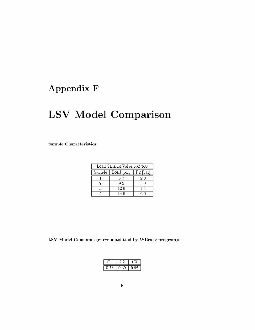
LSV Model Comparison

Sample Characteristics:

Load Sensing Valve 302 360

Sample Load [ton] P2 [bar]

1 5.7 2.02 9.5 3.03 12.0 4.44 14.0 6.0

LSV Model Constants (curve auto�tted by WBrake program):

C1 C2 C3

5.75 0.59 0.98

F

Comparative Plot:

0

1

2

3

4

5

6

2 4 6 8 10 12 14

P2

[bar

]

L [ton]

P1 = 6.0 bar

6*(1-(1/(C1*log(1+C2))*log(1+C2*(C3*(Lopen-L)))))302 360