calculating the effective permeability of sandstone with...

RESEARCH PAPER

Calculating the effective permeability of sandstone withmultiscale lattice Boltzmann/finite element simulations

Joshua A. White Æ Ronaldo I. Borja Æ Joanne T. Fredrich

Received: 1 September 2006 / Accepted: 10 October 2006 / Published online: 18 November 2006� Springer-Verlag 2006

Abstract The lattice Boltzmann (LB) method is an

efficient technique for simulating fluid flow through

individual pores of complex porous media. The ease

with which the LB method handles complex boundary

conditions, combined with the algorithm’s inherent

parallelism, makes it an elegant approach to solving flow

problems at the sub-continuum scale. However, the

realities of current computational resources can limit

the size and resolution of these simulations. A major

research focus is developing methodologies for upscal-

ing microscale techniques for use in macroscale prob-

lems of engineering interest. In this paper, we propose a

hybrid, multiscale framework for simulating diffusion

through porous media. We use the finite element (FE)

method to solve the continuum boundary-value prob-

lem at the macroscale. Each finite element is treated as a

sub-cell and assigned permeabilities calculated from

subcontinuum simulations using the LB method. This

framework allows us to efficiently find a macroscale

solution while still maintaining information about

microscale heterogeneities. As input to these simula-

tions, we use synchrotron-computed 3D microtomo-

graphic images of a sandstone, with sample resolution

of 3.34 lm. We discuss the predictive ability of these

simulations, as well as implementation issues. We also

quantify the lower limit of the continuum (Darcy) scale,

as well as identify the optimal representative elementary

volume for the hybrid LB–FE simulations.

Keywords Finite elements � Lattice Boltzmann �Multiscale simulation � Porous media � Synchrotron

microtomography � Upscaling

1 Introduction

Quantifying the permeability of geomaterials poses a

challenging task to the mathematical modeler because

this parameter depends strongly on the extremely

heterogeneous and complex microstructure of such

materials [5, 13–16, 18, 21, 22, 30, 31]. In addition to

porosity, the effective permeability of geomaterials

depends on pore geometry and connectivity, tortuosity

of flow, the presence of stagnant pockets created, for

example, by dead-end pores, and the degree of satu-

ration [5]. Microstructural changes induced by com-

paction or dilation banding could alter the effective

overall permeability of the medium by several orders

of magnitude [3, 4, 26, 27]. The presence of fissures in a

porous rock can induce preferential flow directions, so

that when viewed as a continuum the flow properties

could exhibit strong anisotropy [26, 27]. Unless we

resort to statistical simulations (see e.g., [1]), limita-

tions of continuum mechanics descriptions that have

been the cornerstone of many flow models inhibit our

ability to incorporate all of these microscale factors in

quantifying the effective permeability of geomaterials.

J. A. White � R. I. Borja (&)Department of Civil and Environmental Engineering,Stanford University, Stanford, CA 94305, USAe-mail: [email protected]

J. T. FredrichSandia National Laboratories,Albuquerque, NM 87185-0751, USA

Present Address:J. T. FredrichExploration and Production Technology Group,BP America, Inc., Houston, TX 77079, USA

123

Acta Geotechnica (2006) 1:195–209

DOI 10.1007/s11440-006-0018-4

Recent advances in high resolution 3D imaging offer

unparalleled opportunities for predicting macroscopic

properties of earth materials from microstructural

measurements [2, 4, 14, 15, 24, 29]. High-resolution 3D

synchrotron computed microtomographic experiments

provide micron-scale image resolution that is superior

to conventional X-ray computed tomography (CT).

The trade-off is that samples are correspondingly

small, approaching millimeters in diametric dimensions

for optimal image resolution. However, despite the

minute size of the specimen the technology provides

significant information on the microscopic structure of

complex porous media.

The past decade has also seen remarkable progress

in the numerical modeling of fluid flow processes at

the pore scale. One of the most promising techniques

is the lattice Boltzmann (LB) method [6, 13, 14, 16–

20, 23, 30, 32]. The LB approach considers a typical

volume element of fluid as composed of a collection

of particles that are represented in terms of a velocity

distribution function at each point in space. The LB

method utilizes nearest neighbor information, so it is

ideally suited for massively parallel computers. The

approach provides insight into the internal velocity

and kinetic energy distributions at the pore scale, and

can detect preferential flow paths and channeling

phenomenon not possible with any available contin-

uum flow models. Direct LB simulation on micron-

scale 3D image data thus offers a significant potential

for new fundamental insights and understanding of

fluid flow processes in a material with a complex

microstructure.

There are, however, potential concerns in any direct

numerical simulation, whether it be fluid flow, wave

propagation, electric transport, or others. In the first

place, such calculations are time-consuming and ex-

tremely memory intensive. For example, a typical LB

sparse storage scheme requires about 100 bytes/fluid-

cell. Therefore, a 3D volume at 30% porosity and

modeled with 10003 cells would require 30 Gb of

memory to store the relevant information throughout

the simulation. This storage space is well beyond the

capability of a typical workstation. Secondly, macro-

scopic properties are often measured by averaging

microscopic quantities over the domain. In many cases,

however, one is not only interested in a single global

value, but also in the spatial variation of the continuum

quantity. For example, in the region of a deformation

band there could be pervasive heterogeneity in the

permeability field, even in a very ‘‘small’’ specimen [3,

4, 7]. A simple global averaging approach masks the

complexity of these spatial variations by smearing

them through the specimen.

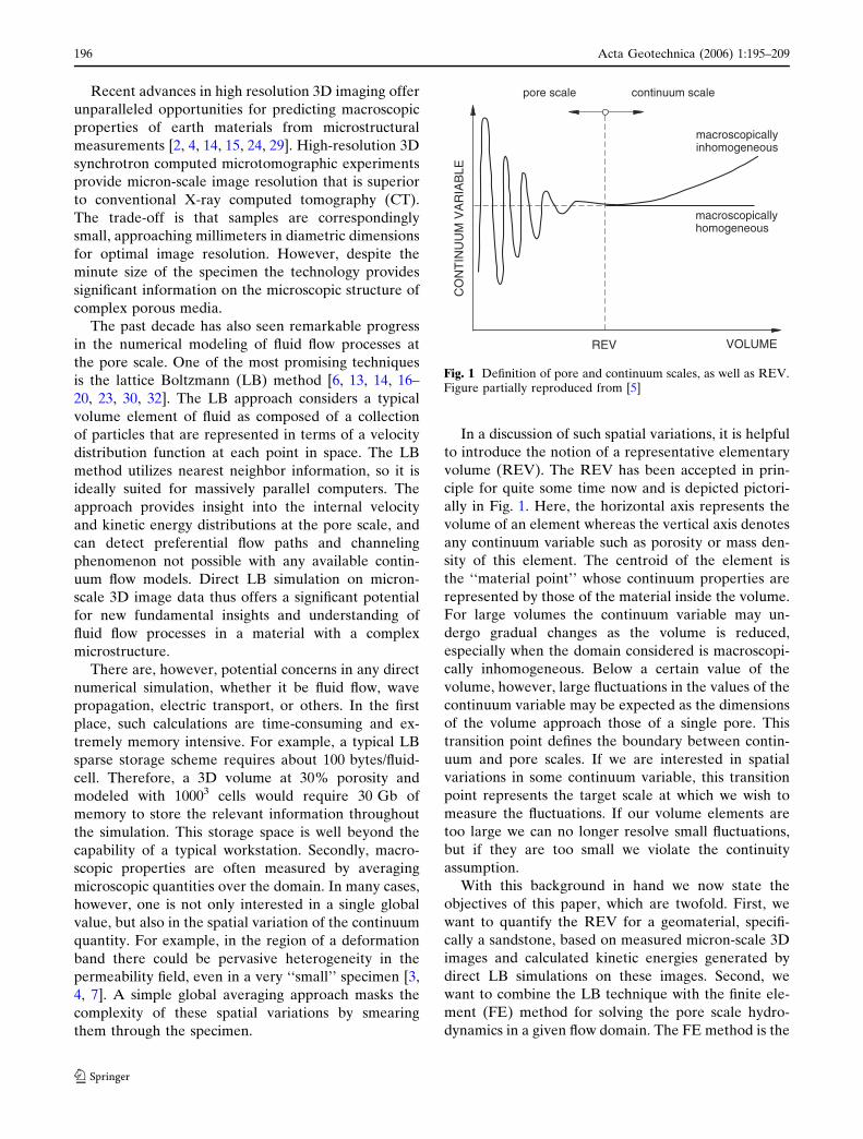
In a discussion of such spatial variations, it is helpful

to introduce the notion of a representative elementary

volume (REV). The REV has been accepted in prin-

ciple for quite some time now and is depicted pictori-

ally in Fig. 1. Here, the horizontal axis represents the

volume of an element whereas the vertical axis denotes

any continuum variable such as porosity or mass den-

sity of this element. The centroid of the element is

the ‘‘material point’’ whose continuum properties are

represented by those of the material inside the volume.

For large volumes the continuum variable may un-

dergo gradual changes as the volume is reduced,

especially when the domain considered is macroscopi-

cally inhomogeneous. Below a certain value of the

volume, however, large fluctuations in the values of the

continuum variable may be expected as the dimensions

of the volume approach those of a single pore. This

transition point defines the boundary between contin-

uum and pore scales. If we are interested in spatial

variations in some continuum variable, this transition

point represents the target scale at which we wish to

measure the fluctuations. If our volume elements are

too large we can no longer resolve small fluctuations,

but if they are too small we violate the continuity

assumption.

With this background in hand we now state the

objectives of this paper, which are twofold. First, we

want to quantify the REV for a geomaterial, specifi-

cally a sandstone, based on measured micron-scale 3D

images and calculated kinetic energies generated by

direct LB simulations on these images. Second, we

want to combine the LB technique with the finite ele-

ment (FE) method for solving the pore scale hydro-

dynamics in a given flow domain. The FE method is the

VOLUME

CO

NT

INU

UM

VA

RIA

BLE

macroscopicallyinhomogeneous

macroscopicallyhomogeneous

continuum scalepore scale

REV

Fig. 1 Definition of pore and continuum scales, as well as REV.Figure partially reproduced from [5]

196 Acta Geotechnica (2006) 1:195–209

123

most widely used continuum model for the numerical

analysis of complex boundary-value problems, and its

marriage with the LB technique offers unique oppor-

tunities for attacking the pore scale problem in a truly

multiscale way. The proposed hybrid modeling tech-

nique delivers at least two potential benefits. First,

because the domain of the LB simulations is reduced to

the smallest REV scale, LB calculations now become

significantly cheaper and less memory intensive (the

cost of the FE calculations is almost nil compared to

the cost of the LB simulations). Second, inhomogene-

ities of the macroscale variables such as the effective

permeability can now be quantified in the flow domain.

These benefits can be realized more clearly in 3D

simulations as we shall demonstrate with Castlegate

sandstone.

2 Description of LB–FE model

The challenging aspect of flow in porous media is that

the governing equations shift as one moves from one

length scale to the next. At the macroscale, we are

interested in solving the diffusion equation in the do-

main of interest, subject to specified boundary condi-

tions. We can readily solve this problem using a variety

of continuum methods (e.g., FE), but first we must

have some idea of the permeability of the porous

medium. This permeability, however, is an averaged

representation of complex solid–fluid interactions

occurring at a smaller scale. Typical continuum meth-

ods have no way of probing the pore scale to determine

the required permeability field. As a result, we typi-

cally turn to experimental data or simple analytical

relations.

As we look one level down, the flow through indi-

vidual pores is governed by the Navier–Stokes equa-

tions, whose solution we may recover using LB. In

principle, we could just use a very large LB simulation

to obtain the macroscopic solution we wanted in the

first place, but we are limited by the realities of current

computational resources. Beyond a certain volume, it

becomes impractical to discretize every pore with suf-

ficient fidelity and solve for the complete flow field.

The question we attempt to address in this work is

whether we can apply a multiscale approach to sidestep

the inherent difficulties of the single-scale methods just

described. We instead propose a hybrid method that

combines the advantages of both LB and FE methods.

In the macroscopic domain, we solve the diffusion

equation on a FE mesh. Instead of using experimental

data to calibrate the permeability field, we perform a

small LB simulation within each element to examine the

microstructure and assign an appropriate permeability

tensor. Thus we are able to incorporate information

about microscale interactions into our continuum

picture. Simultaneously, we limit the computational

requirements by running the expensive LB simulations

in a series of small domains instead of one large one. In

this way, we approach the solution from a perspective

which is appropriate to the multiscale nature of the

problem. Our goal in the next few sections is to establish

the details of this framework.

We would like to emphasize, however, that the

proposed framework is by no means a replacement for

detailed LB simulations. We have approached the

problem from a continuum perspective, in which we

are interested in the macroscopic effects of microscale

behavior. Our simulations, however, do not resolve the

details of the flow field in every pore. In many cases,

these details might be the primary objective of the

simulation—perhaps in an investigation of trapping

phenomena or mixing behavior. As such, a detailed LB

simulation may be appropriate and necessary. Our

perspective in this paper, however, is that the LB

method is a powerful microscale technique, but scales

poorly when one is interested in field-scale solutions.

2.1 Lattice Boltzmann technique

The lattice Boltzmann technique is uniquely suited to

modeling the complexities of fluid flow through disor-

dered media, including flow through porous geomate-

rials [2, 13, 14, 16, 18, 19, 21]. Given the ease with

which the method handles complex internal bound-

aries, LB is a natural choice for our microscale simu-

lations. In the following, we provide a brief description

for the unfamiliar reader. Several excellent references

that review the development and details of the LB

method may be found in the literature, including [10,

28].

In LB, we do not solve the Navier–Stokes (NS)

equations directly, but rather a discretization of the

Boltzmann equation is formulated such that the

velocity and pressure fields satisfy the NS equations. In

our computations the two-phase microstructure of the

porous medium is represented as a bitmap image, in

which each pixel (in 2D) or voxel (in 3D) represents

either solid or void. Each void pixel is assigned a node,

and the pore-space is represented by a lattice con-

necting each of these nodes. A typical unit cell for the

lattice is illustrated in the appendix. The unknown

quantities at each node are not velocity and pressure,

but rather a discrete distribution function fi(x,t).

This function represents the probability of finding a

particle at location x and time t moving with a certain

Acta Geotechnica (2006) 1:195–209 197

123

discrete velocity ei. These discrete velocities point

along the inter-node links in the lattice. The particle

distribution satisfies the discrete-velocity Boltzmann

equation,

@fi

@tþ ei � rfi ¼ Xi; ð1Þ

where Wi is a collision term that accounts for the net

addition of particles moving with velocity ei due to

inter-particle collisions. Once we solve for the particle

distribution function, quantities such as density, pres-

sure, and velocity may be recovered from the first two

moments of these distributions. In our implementation

we solve a discretized version of Eq. 1 using the line-

arized Bhatnagar, Gross, and Krook (LBGK) scheme

[6] on D2Q9 and D3Q19 lattices [23]. Internal solid-

fluid boundaries have been handled using the popular

‘‘bounce-back’’ rule. It should be noted that much re-

cent work has focused on improved hydrodynamic

boundary conditions [17, 20, 32], accelerating conver-

gence [30], and on other improvements to the standard

methods. Our goal in this work is not to focus on these

details, but rather outline a multiscale framework. Our

methodology is by no means limited to the particular

features chosen here.

In the hybrid LB–FE model, the global domain is

divided into a series of rectilinear sub-cells, each of

which will become a finite element. To determine the

local permeability in each sub-cell, we are interested in

solving for the steady-state flow field v(x) resulting

from a hydraulic gradient �h applied along basis

direction ej. For now, let us temporarily postpone the

discussion of the imposed sub-cell boundary condi-

tions. With the velocity field determined, we may re-

cover the jth column of the element permeability

tensor k according to

kij ¼ � vi xð Þh i lrhð Þj

; ð2Þ

where l is the kinematic viscosity, and Æ...æ denotes a

volume average over the domain. One could also

measure the specific discharge through a single plane

to determine the permeability; both methods produce

the same results. To determine the complete tensor, a

separate simulation must be run along each basis

direction ej—i.e., two in 2D and three in 3D.

We return now to the issue of boundary conditions

for the sub-cell simulations. The primary assumption

we have made in dividing the domain into individual

sub-cells is that the element permeability can be

approximated with no knowledge of neighbor cells—

i.e., a locality assumption. We therefore need to

impose boundary conditions that will reasonably mimic

the flow situation in the complete porous medium. In

this work, we have adopted periodic conditions in

which the particle distributions leaving one side of the

domain re-enter at the opposite plane. The element is

therefore treated as a unit cell in an infinite domain.

The hydraulic gradient is then imposed using a body

force scheme by exploiting the fact that force is equal

to change in momentum. During each time step, we

add additional density to the forward-pointing particle

distributions, while subtracting the same from the

backward directions. This does not alter the total

density at the node, but adds a constant amount of

momentum in the positive direction.

By using a periodic scheme, however, we encounter

the additional geometric restriction that the solid-void

geometry on the outgoing face must match the geo-

metry on the incoming face. This difficulty is readily

overcome by simply mirroring the domain in all

directions. If this is done explicitly, however, the lattice

size grows by a factor of four in 2D, and eight in 3D. A

scheme for side-stepping this difficulty and implicitly

mirroring the domain, while still working on the ori-

ginal size lattice, has been presented in [14]. We have

employed this scheme for our 3D simulations, with

significant computational savings. In 2D the computa-

tional requirements were not stringent, and the simpler

explicit scheme was used.

2.2 Finite element technique

Having solved for the local element tensors, we may

assign the appropriate permeability at every Gauss

point in the global finite element mesh. A straight-

forward solution of the diffusion equation, using a

standard Galerkin formulation, yields the desired

macroscopic pressure field. Compared with the LB

simulations, the additional computational time re-

quired by the FE solution is negligible.

Our FE implementation contains one unusual

feature, however. In the standard formulation of the

diffusion equation, the permeability tensor is assumed

symmetric. This then leads to a symmetric, positive

definite stiffness matrix after assembly. In our sub-cell

LB simulations, however, the measured permeability

tensors are not symmetric, leading to an asymmetric

stiffness matrix and requiring an appropriate linear

solver [8]. In the numerical examples to follow, we

explore the effect this asymmetry has on the solution

by comparing results to cases when (a) the tensor has

been symmetrized, and (b) the tensor has been

assumed isotropic.


123

2.3 Boundary between micro- and Darcy scales

A crucial step for the hybrid framework is determining

an appropriate FE discretization. By choosing a very

coarse mesh, we are forced to do expensive LB simu-

lations on each finite element (treated as a sub-cell)

and lose a great deal of computational efficiency. By

choosing a highly refined FE mesh, on the other hand,

we could get into the range of the pore scale where

continuum approximations clearly are inappropriate.

The challenge, then, is to find a method to quantify this

transition from pore scale to continuum scale behavior.

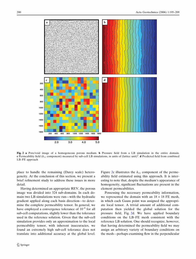
Returning to Fig. 1, we propose that the onset of the

continuum scale be quantified by observing the fluc-

tuations in the behavior of an energy measure—the

local rate of mechanical dissipation:

DðxÞ ¼ ð2lÞ�ij�ij; �ij ¼1

2vj;i þ vi;j

� �; ð3Þ

where �ij is the symmetric gradient of the velocity field.

As pointed out by Pilotti et al. [22], energy dissipation

governs the evolution of the total head, and thus is

closely linked to the absolute permeability of the

medium. As such, it can provide a meaningful indicator

of the onset of the Darcy scale, unlike other macro-

scale variables such as porosity which are insufficient to

describe the permeability of an arbitrary porous med-

ium [5]. If we choose a REV such that the dissipation

behaves as a continuum variable, one expects that any

quantity that depends on it will also behave as a con-

tinuum variable.

In the next two sections, we present numerical re-

sults using the hybrid LB–FE framework we have

established to clarify this discussion. We begin with

three 2D examples with artificially generated porous

media. We conclude with a 3D example based on

microtomographic images of an actual sandstone.

3 Two-dimensional examples

Our first 2D example is a macroscopically homoge-

neous porous medium (Fig. 2). The binary pore/void

image consists of 18002 pixels (Fig. 2a). To obtain a

reference solution, we performed a LB simulation in

the entire domain. A constant pressure was assigned

along the left and right boundaries, and a no flow

condition was imposed on the other two edges. The

question of how best to assign pressure boundary

conditions in the LB technique has prompted several

studies [17, 20, 32]. We have adopted an approach

based on the work of Zou and He [32] for the D2Q9

lattice. In an appendix we present a formulation for the

D3Q19 lattice. The assigned pressure drop was kept

small enough for the flow to remain in the low Rey-

nold’s number regime and ensure Darcy’s law remains

valid. With boundary conditions established, the LB

simulation was run until steady state was reached. Our

criteria for convergence was based upon the rate of

change of the velocity field, with a convergence toler-

ance of 10–7. This value was found sufficient to guar-

antee that the flow field had reached steady state.

Figure 2b illustrates the resulting pressure field, an

essentially linear head drop from inlet to outlet.

Having solved for the velocity field within the pore

space, we can calculate the local rate of mechanical

dissipation at each point using Eq. 3. In analogy to

Fig. 1, we then averaged this property over increas-

ingly large volumes (Fig. 3). In the figure, the volume is

represented by its side length s, normalized by the full

domain dimension L. For small element dimensions,

we see dramatic fluctuations in the averaged property,

indicative of the dominance of microscale behavior. As

the volume is increased, however, these oscillations

reduce dramatically and indicate the onset of what we

would consider the macroscale. Figure 3 thus provides

a meaningful way of determining how large an REV is

necessary for the continuum assumption to be valid.

We note, however, that the measured dissipation will

also depend on where in the sample the averaging

volume is located. Therefore, it makes sense to sample

at several different points in the domain in order to

obtain a more complete picture of the fluctuation

behavior.

It should be noted that we are at an advantage in

having a reference solution in a large domain in order

to develop Fig. 3. In practice one would most likely

take an incremental approach, beginning with some

small dimension and running increasingly large LB

simulations until confident that the continuum scale

had been reached. In either case, observing the aver-

aged behavior of the dissipation, or some other mea-

sure of interest, can provide a quantitative way to

evaluate this scale transition.

Based on the previous discussion, we felt that an

18 · 18 discretization of the flow domain would yield

sub-cells of sufficient size to be treated as REVs.

Again, our discretization criteria is to choose sub-cells

as small as possible to gain the greatest computational

advantage, but not so small that we violate the neces-

sary continuum assumption at the FE level. Never-

theless, it is not necessary to find an REV sufficiently

large that all oscillations have disappeared. Rather, we

are merely interested in avoiding the dramatic micro-

scale oscillations. The finite element solution is then in


123

place to handle the remaining (Darcy scale) hetero-

geneity. At the conclusion of this section, we present a

brief refinement study to address these issues in more

detail.

Having determined an appropriate REV, the porous

image was divided into 324 sub-domains. In each do-

main two LB simulations were run—with the hydraulic

gradient applied along each basis direction—to deter-

mine the complete permeability tensor. In general, we

have employed a convergence tolerance of 10–6 for all

sub-cell computations, slightly lower than the tolerance

used in the reference solution. Given that the sub-cell

simulation provides only an approximation to the local

permeability tensor, with inherent inaccuracies, we

found an extremely high sub-cell tolerance does not

translate into additional accuracy at the global level.

Figure 2c illustrates the k11 component of the perme-

ability field estimated using this approach. It is inter-

esting to note that, despite the medium’s appearance of

homogeneity, significant fluctuations are present in the

element permeabilities.

Possessing the necessary permeability information,

we represented the domain with an 18 · 18 FE mesh,

in which each Gauss point was assigned the appropri-

ate local tensor. A trivial amount of additional com-

putation then yielded the global solution for the

pressure field, Fig. 2d. We have applied boundary

conditions on the LB–FE mesh consistent with the

reference LB solution. One should recognize, however,

that having determined the permeability field we may

assign an arbitrary variety of boundary conditions on

the mesh—perhaps examining flow in the perpendicular

200 400 600 800 1000 1200 1400 1600 1800

200

400

600

800

1000

1200

1400

1600

1800

2.0 3.0 4.0 5.0

a

dc

b

200 400 600 800 1000 1200 1400 1600 1800

200

400

600

800

1000

1200

1400

1600

1800

2.0 3.0 4.0 5.0

a

dc

b

Fig. 2 a Pore/void image of a homogeneous porous medium. b Pressure field from a LB simulation in the entire domain.c Permeability field (k11 component) measured by sub-cell LB simulations, in units of (lattice unit)2. d Predicted field from combinedLB–FE approach


123

direction, or some source-to-sink behavior. In contrast,

the invested computational work in the pure LB ap-

proach only yields a single solution.

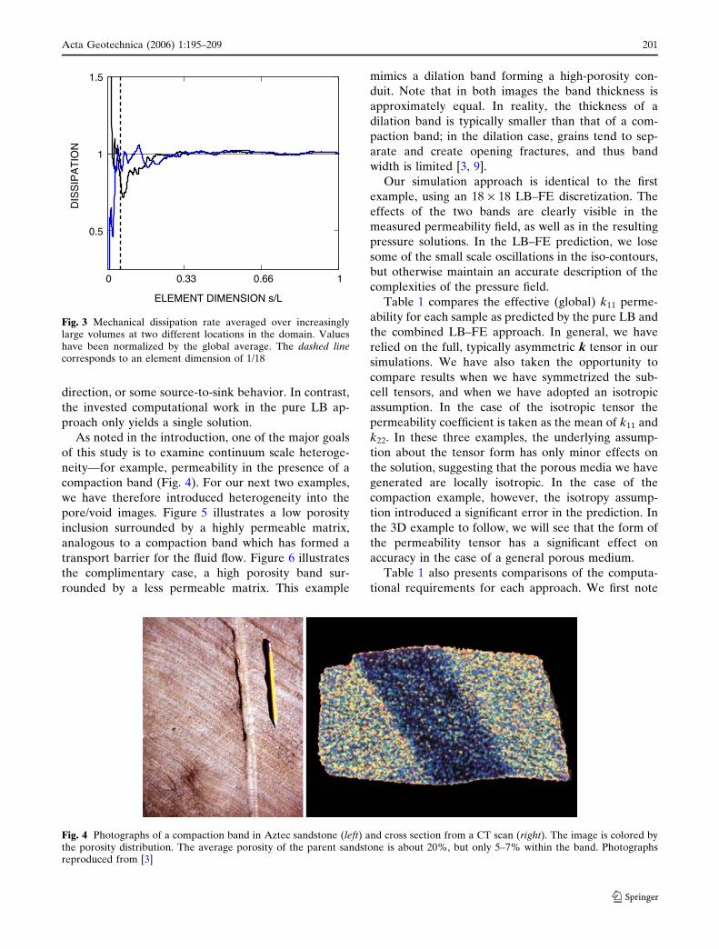
As noted in the introduction, one of the major goals

of this study is to examine continuum scale heteroge-

neity—for example, permeability in the presence of a

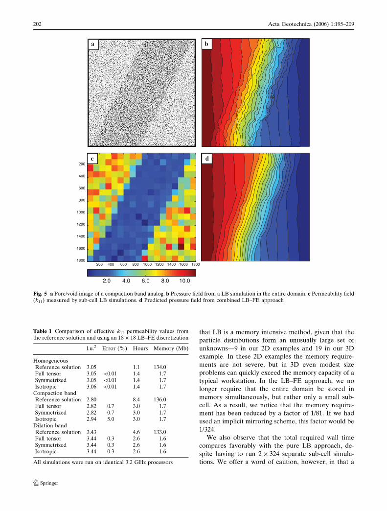
compaction band (Fig. 4). For our next two examples,

we have therefore introduced heterogeneity into the

pore/void images. Figure 5 illustrates a low porosity

inclusion surrounded by a highly permeable matrix,

analogous to a compaction band which has formed a

transport barrier for the fluid flow. Figure 6 illustrates

the complimentary case, a high porosity band sur-

rounded by a less permeable matrix. This example

mimics a dilation band forming a high-porosity con-

duit. Note that in both images the band thickness is

approximately equal. In reality, the thickness of a

dilation band is typically smaller than that of a com-

paction band; in the dilation case, grains tend to sep-

arate and create opening fractures, and thus band

width is limited [3, 9].

Our simulation approach is identical to the first

example, using an 18 · 18 LB–FE discretization. The

effects of the two bands are clearly visible in the

measured permeability field, as well as in the resulting

pressure solutions. In the LB–FE prediction, we lose

some of the small scale oscillations in the iso-contours,

but otherwise maintain an accurate description of the

complexities of the pressure field.

Table 1 compares the effective (global) k11 perme-

ability for each sample as predicted by the pure LB and

the combined LB–FE approach. In general, we have

relied on the full, typically asymmetric k tensor in our

simulations. We have also taken the opportunity to

compare results when we have symmetrized the sub-

cell tensors, and when we have adopted an isotropic

assumption. In the case of the isotropic tensor the

permeability coefficient is taken as the mean of k11 and

k22. In these three examples, the underlying assump-

tion about the tensor form has only minor effects on

the solution, suggesting that the porous media we have

generated are locally isotropic. In the case of the

compaction example, however, the isotropy assump-

tion introduced a significant error in the prediction. In

the 3D example to follow, we will see that the form of

the permeability tensor has a significant effect on

accuracy in the case of a general porous medium.

Table 1 also presents comparisons of the computa-

tional requirements for each approach. We first note

0 0.33 0.66 1

0.5

1

1.5

ELEMENT DIMENSION s/L

DIS

SIP

AT

ION

Fig. 3 Mechanical dissipation rate averaged over increasinglylarge volumes at two different locations in the domain. Valueshave been normalized by the global average. The dashed linecorresponds to an element dimension of 1/18

Fig. 4 Photographs of a compaction band in Aztec sandstone (left) and cross section from a CT scan (right). The image is colored bythe porosity distribution. The average porosity of the parent sandstone is about 20%, but only 5–7% within the band. Photographsreproduced from [3]


123

that LB is a memory intensive method, given that the

particle distributions form an unusually large set of

unknowns—9 in our 2D examples and 19 in our 3D

example. In these 2D examples the memory require-

ments are not severe, but in 3D even modest size

problems can quickly exceed the memory capacity of a

typical workstation. In the LB–FE approach, we no

longer require that the entire domain be stored in

memory simultaneously, but rather only a small sub-

cell. As a result, we notice that the memory require-

ment has been reduced by a factor of 1/81. If we had

used an implicit mirroring scheme, this factor would be

1/324.

We also observe that the total required wall time

compares favorably with the pure LB approach, de-

spite having to run 2 · 324 separate sub-cell simula-

tions. We offer a word of caution, however, in that a

200 400 600 800 1000 1200 1400 1600 1800

200

400

600

800

1000

1200

1400

1600

1800

2.0 4.0 6.0 8.0 10.0

a b

c d

Fig. 5 a Pore/void image of a compaction band analog. b Pressure field from a LB simulation in the entire domain. c Permeability field(k11) measured by sub-cell LB simulations. d Predicted pressure field from combined LB–FE approach

Table 1 Comparison of effective k11 permeability values fromthe reference solution and using an 18 · 18 LB–FE discretization

l.u.2 Error (%) Hours Memory (Mb)

HomogeneousReference solution 3.05 1.1 134.0Full tensor 3.05 <0.01 1.4 1.7Symmetrized 3.05 <0.01 1.4 1.7Isotropic 3.06 <0.01 1.4 1.7

Compaction bandReference solution 2.80 8.4 136.0Full tensor 2.82 0.7 3.0 1.7Symmetrized 2.82 0.7 3.0 1.7Isotropic 2.94 5.0 3.0 1.7

Dilation bandReference solution 3.43 4.6 133.0Full tensor 3.44 0.3 2.6 1.6Symmetrized 3.44 0.3 2.6 1.6Isotropic 3.44 0.3 2.6 1.6

All simulations were run on identical 3.2 GHz processors


123

strict comparison of the two times is ambiguous. The

LB–FE approach provides a full characterization of the

permeability field and allows one to solve additional

boundary-value problems with trivial additional com-

putational effort. This is not the case with a simple LB

solution. We also note that our LB implementation

does not take advantage of several methods available

for accelerating convergence, such as the method of

Verberg and Ladd [30]. Interestingly, this method has

even larger memory requirement than the standard LB

algorithm (on the order of 50% extra) so that savings

in computational time are balanced by the need for

greater memory. Utilizing the framework presented

here, however, one might take advantage of both im-

proved convergence and dramatic memory savings.

We conclude this section with a brief refinement

study based on the homogeneous example, to illustrate

the importance of choosing a proper discretization.

Figure 7 illustrates the relative error in the predicted

sample permeability for a large range of element sizes.

Above an element dimension of 1/18, the REV size we

identified using our dissipation methodology, we see

that the relative error remains bounded below 2%. The

striking feature of this graph, however, is the solution

behavior as one chooses extremely small elements. We

notice a sharp jump in error, indicating that the ele-

ments are no longer sufficiently large to be represen-

tative, and are dominated by large microscale

fluctuations in element properties.

There is one further observation to be made con-

cerning REVs for anisotropic media. The defining

characteristic of anisotropy is the fact that in different

directions different percolating pathways are activated,

and the primary transport mechanisms may change

radically. A typical example would be a medium

containing a series of subparallel fractures that may

200

400

600

800

1000

1200

1400

1600

1800

2.0 4.0 6.0 8.0 10.0 12.0

a

dc

b

200 400 600 800 1000 1200 1400 1600 1800

Fig. 6 a Pore/void image for a dilation band analog. b Pressure field from reference solution. c Permeability field (k11) measured bysub-cell LB simulations. d Predicted pressure field from combined LB–FE approach


123

become active or inactive depending on the local

hydraulic gradient. Thus, when dealing with such

anisotropy, there is no reason to expect that the REV

for a particular flow direction corresponds to the nec-

essary REV for an alternative flow direction. There-

fore, care should be taken when determining the

necessary element size such that the chosen REV is

appropriate for the entire suite of problems to be

modeled.

4 Castlegate sandstone

To this point, our examples have all been artificially

generated. In practice, however, one would most likely

be interested in 3D simulations based on actual geo-

logic microstructures. To this end, we conclude our

numerical examples with an example based on real

data from a natural sandstone sample from the Cast-

legate Formation (Cretaceous Mesa Verde Group,

eastern Utah). This fine- to medium-grained (~0.2 mm

grain size) sandstone is commonly used in experimen-

tal rock mechanics studies as an analogue reservoir

rock. A detailed description of the phase distribution is

provided in [11, 12]. Figure 8 presents an image of the

solid phase of the sandstone specimen. As reported by

Fredrich et al. [14], data for several sandstone samples

was originally collected using synchrotron microto-

mography at the Argonne Advanced Photon Source

and passed through a series of post-processing steps to

produce the final microtomographic images. A syn-

chrotron provides a high-energy, monochromatic X-

ray source that avoids many of the disadvantages of

standard X-ray tomography techniques such as beam

hardening [14, 24, 25]. As a result, one is able to gather

high-resolution, high-quality images. The drawback is

that sample sizes are correspondingly small. The image

resolution for this Castlegate sample is 3.34 lm, while

the overall sample volume is 1.4 mm3.

Fredrich et al. then ran detailed LB simulations

based on the resulting images. They compared the

predicted permeability with laboratory permeametry

experiments performed on centimeter-scale cores from

the same specimens, finding excellent agreement

among all samples. The permeability of Castlegate

sandstone has been well-characterized experimentally

by several authors, and generally falls in the range 0.8–

1.2 lm2. The LB simulations of the Castlegate samples

fell in the range 0.8–1.0 lm2. Given the demonstrated

ability of the LB method to predict macroscale per-

meability, we wished to see if we could get similar

results using a combined LB–FE approach.

As before, we ran a reference LB simulation in the

entire domain of our specimen. Constant pressure

conditions were specified on an inlet and outlet face,

and normal flow was prevented along the other four

boundaries. We interject that these boundary condi-

tions are an arbitrary choice, and one can imagine a

variety of other configurations for an upscaling study.

Several have been presented in the literature, with

advantages and disadvantages to each. Our purpose

here is not to advocate a particular choice, but rather

compare two methods in which consistent conditions

0 0.1 0.2 0.30

5

10

15

20

25

30


ER

RO

R %

Fig. 7 Mesh refinement study for the homogeneous example.Data points represent relative error in predicted effectivepermeability, based on the reference LB solution

Fig. 8 Microtomographic image of the solid phase of a Castle-gate sandstone. Image resolution is 3.34 lm. Image volume is1.4 mm3. Image reproduced from [14]


123

have been applied. Our pressure formulation is de-

tailed in an appendix. The computation was run in

parallel on eight processors of a distributed memory

cluster, with steady state reached after approximately

26 h (206 h of total wall time). Again, we used the

resulting velocity field to calculate the local rate of

mechanical dissipation, and averaged it over increas-

ingly large volumes (Fig. 9). From this analysis, we

determined that a 3 · 3 · 3 discretization of the do-

main would yield appropriately sized REVs. Figure 10

illustrates the FE mesh and boundary conditions we

have used. We note that oscillations in the dissipation

graph are fairly sizeable even as one approaches the

global sample size. This is not surprising given the

extremely small sample dimensions. Nevertheless, we

will see that reasonable results can be achieved despite

seemingly large fluctuations.

With the domain thus divided into 27 elements, 81

separate sub-cell simulations were required to deter-

mine the 27 local permeability tensors. Table 2 pro-

vides the complete tensor for a few typical elements,

which display significant asymmetry and anisotropy.

Table 3 compares the predicted effective k11 perme-

ability of the sandstone sample. Our predicted per-

meability value of 0.89 lm2 is in agreement with both

the full LB solution and with the experimental range

presented earlier. Again, we have also presented re-

sults based on the tensor form: asymmetric, symme-

trized, and isotropic. Using the full, asymmetric tensor

provides the best solution, with errors increasing as one

introduces symmetry and isotropy assumptions. These

results suggest that, in practice, the full tensor is most

appropriate. We also observe a significant execution

speedup and dramatic savings in required memory. It

appears then that the LB–FE methodology provides a

reasonable method for estimating a macroscale per-

meability value in a computationally efficient manner.

5 Closure

Several key issues have been addressed in this paper.

The first and foremost revolves around the notion of

the effective permeability as it applies to an REV. The

REV is the boundary between the micro-scale and

Darcy scale, and as such it represents the smallest

volume over which a granular material with a complex

microstructure may be considered a continuum. Al-

though the notion of an REV has been accepted in

principle, it is challenging to quantify in practice. In

this paper we used the local rate of mechanical dissi-

pation to quantify the REV for an actual sandstone,

not only for calculating its overall effective perme-

ability but also for describing how this very important

material parameter varies spatially throughout the

sample. Clearly, the spatial distribution of effective

permeability provides much more information than the

overall permeability itself, even if the volume of

interest is only 1.4 mm3.

None of these ideas would be useful in practice

without the recent advances in high resolution 3D

imaging and powerful numerical modeling techniques

currently at our disposal. High resolution 3D syn-

chrotron-computed microtomography combined with

the powerful lattice Boltzmann-finite element hybrid

method is an enviable combination to attack the pore

scale hydrodynamics problem. The proposed LB–FE

0 0.33 0.66 10

1

2

3

4


DIS

SIP

AT

ION

Fig. 9 Mechanical dissipation rate averaged over increasinglylarge volumes at two different locations in the domain,normalized with respect to the global average

INFLOW

12

3

OUTFLOW

NO FLOW

NO FLOW

3

2

1

6

5

4

9

8

7

Fig. 10 3 · 3 · 3 FE discretization used in the Castlegateexample. Normal flow is prevented along shaded boundaries


123

technique has dual advantages in that it not only

quantifies the spatial variation of effective permeabil-

ity, it also reduces the computing time and memory

requirements. Hybrid techniques are by no means un-

ique, but to the knowledge of the authors this is the

first time that the combined LB–FE methods have

been used for pore scale hydrodynamics on very high-

resolution images. As an aside, we noted that the full

(asymmetric) effective permeability tensor enhances

the accuracy of the LB–FE approach particularly in 3D

simulations. Other challenges ahead include enhancing

the performance of the LB–FE technique and devel-

oping more robust computational platforms for up-

scaling the modeling further to field dimensions.

Acknowledgments The first author gratefully acknowledges thesupport of a Stanford Graduate Fellowship, a National ScienceFoundation Graduate Research Fellowship, and two summerGraduate Research Internships at Sandia National Laboratories.The second author acknowledges the support of the U.S.Department of Energy Grant DE-FG02-03ER15454, and theU.S. National Science Foundation, Grant CMS-0324674. Thefirst and third author acknowledge support from the U.S.Department of Energy, Office of Basic Energy Sciences,Chemical Sciences and Geosciences Program. Portions of thiswork were performed at Sandia National Laboratories funded bythe US DOE under Contract DE-AC04-94AL85000. Sandia is amultiprogram laboratory operated by Sandia Corporation, aLockheed Martin Company, for the United States Departmentof Energy’s National Nuclear Security Administration. We aregrateful to David Noble of Sandia National Laboratories forhelpful discussions concerning boundary conditions, and toProfessor Atilla Aydin of Stanford University for allowing thereproduction of Fig. 4. We are also grateful to two anonymousreviewers for their constructive comments. Much of the com-putation was performed on Sandia’s 256-node ICC Libertycluster.

Appendix: Pressure boundary condition

In the LB method, pressure and density are related

through the equation of state

Table 2 Element permeability components (lm2) following the numbering scheme noted in Fig. 10

Element k11 k22 k33 k21 k12 k31 k13 k32 k23

1 2.4e-1 2.0e-1 1.5e-1 –2.3e-2 –6.6e-3 3.7e-2 3.5e-2 –3.5e-2 1.5e-12 2.6e-1 5.1e-1 3.3e-1 –6.9e-3 4.2e-2 –1.0e-2 –7.4e-2 –7.9e-3 3.3e-13 8.4e-1 5.1e-1 5.4e-1 –4.3e-1 –1.7e-1 2.8e-1 –6.4e-2 –4.0e-2 5.4e-14 9.6e-1 1.7 5.4e-1 –1.8e-1 –3.0e-1 2.1e-2 –3.2e-2 2.7e-1 5.4e-15 1.2 6.2e-1 7.1e-1 –2.6e-2 4.0e-2 2.6e-1 3.6e-2 9.2e-2 7.1e-127 1.1 9.0e-1 9.5e-1 –2.6e-1 –1.1e-1 –5.0e-2 –3.7e-2 6.1e-2 1.3e-1Average 1.2 8.3e-1 7.9e-1 –5.7e-4 –2.1e-2 4.2e-2 1.9e-3 4.8e-3 –3.5e-2

We have not listed all 27 elements for brevity

Table 3 Castlegate effective k11 permeability values from boththe reference solution and the LB–FE approach

Method lm2 Error(%)

Hours Memory(Mb)

Reference solution 0.893 206.1 1,630Full tensor 0.911 2.0 30.8 60Symmetrized 0.845 5.4 30.8 60Isotropic 0.803 10.1 30.8 60

All simulations were run on identical 3.06 GHz processors

Y

X

Z

X

(17) 4 (18)

(15) 3 (16)

10 8

9 7

(13)2

(14)

(11)1

(12)

(16) 6 (18)

(15) 5 (17)

14 12

13 11

(9)2

(10)

(7)1

(8)

(a) (b)

Fig. 11 a Typical unit cell for a D3Q19 lattice. Rest node is gray, and 18 neighbor nodes are black. Link vectors are omitted for clarity.b Two orthogonal views of the D3Q19 lattice, illustrating the present numbering scheme. Out-of-plane links are noted withparentheses


123

p ¼ c2q; ð4Þ

where c is the speed of sound (for a perfect gas) on the

given lattice. To impose a pressure boundary

condition, we therefore seek to impose a specified

density. Recall that the density q and macroscopic flow

velocity u are defined in terms of the discrete particle

distributions fi and their associated velocities ei,

q ¼X18

i¼0

fi; qu ¼X18

i¼1

fiei: ð5Þ

In our 3D simulations, we have used a D3Q19 lattice

consisting of 18 neighbor links and one rest state.

Figure 11 illustrates the basic lattice unit and the

numbering scheme we have employed.

Consider a typical lattice node located on the inlet

boundary. At this node we assign a density qin, and

further specify uy = uz = 0. Consider now the density

distribution after the streaming step in a typical LB

iteration. Any particle population coming from an

interior node becomes a known quantity. On the other

hand, f1, f7, f8, f11, and f12 remain undetermined since

these populations stream from points outside the do-

main. We therefore seek to determine these five

unknowns such that they satisfy the specified density

and velocity conditions.

To shorten notation let us group the particle popula-

tions into three sets according to whether ex = 1, 0, or –1.

Xþ ¼ f1; 7; 8; 11; 12g: ð6Þ

Xo ¼ f0; 3; 4; 5; 6; 15; 16; 17; 18g: ð7Þ

X� ¼ f2; 9; 10; 13; 14g: ð8Þ

In this notation, any fi 2 X+ is an unknown. Our first

task is to determine the inlet velocity ux in terms of the

known populations. From the density and momentum

equations

qin ¼X

X�fi þ

X

Xo

fi þX

Xþ

fi; ð9Þ

qinux ¼X

Xþ

fi �X

X�fi; ð10Þ

which implies

ux ¼ 1� 1

qin

X

Xo

fi þ 2X

X�fi

" #

: ð11Þ

Now that the complete vector u is determined, our goal

is to find a particle distribution that satisfies Eqs. 5.

These relations, however, are insufficient to determine

the unknown fi uniquely. In light of this fact, we have

adopted an approach like that of Zou and He [32]. We

note that the equilibrium particle distribution also

satisfies the momentum equations,

X18

i¼1

feqi ei ¼ qu: ð12Þ

This implies that the unknown fi must satisfy the fol-

lowing in order to maintain the appropriate x-

momentum:

X

Xþ

fi �X

X�fi ¼

X

Xþ

feqi �

X

X�f

eqi : ð13Þ

Let us denote by �fi the particle population traveling

in the opposite direction to fi; that is, ei and �ei point

in opposite directions. Zou and He noted that by

choosing the unknown fi such that

fi � feqi ¼ �fi � �f

eqi ; ð14Þ

Eq. 13 is automatically satisfied. They described this

approach as a ‘‘bounceback rule‘‘ for the non-

equilibrium distribution, in analogy to the commonly

used bounceback rule for dealing with solid interfaces.

In the D3Q19 model, the equilibrium distributions are

given by

feqi ¼ qxi 1þ 3u � ei þ

9

2ðu � eiÞ2 �

3

2u � u

� �; ð15Þ

with weights xi = 1/3, 1/18, and 1/36 for the rest par-

ticle, nearest neighbor links, and diagonal links,

respectively.

With this simple heuristic in hand, a scheme emerges

for determining the unknown particle populations.

First, we fix the unknown component normal to the

inlet plane,

f1 ¼ f2 þ feq1 � f

eq2

� �¼ f2 þ

1

3qinux: ð16Þ

For the four remaining unknowns, we apply a similar

bounceback rule to ensure that the x-momentum

equation is satisfied. We also note, however, that we

can adjust the y and z-momenta without altering the x-

momentum by using the populations tangential to the

inlet plane, fi 2 Xo. In particular, we choose

f7 ¼ f10 þ1

2f4 þ f17 þ f18ð Þ � 1

2f3 þ f15 þ f16ð Þ þ 1

6qinux;

ð17Þ


123

f8 ¼ f9 �1

2f4 þ f17 þ f18ð Þ þ 1

2f3 þ f15 þ f16ð Þ þ 1

6qinux;

ð18Þ

f11 ¼ f14 þ1

2f6 þ f16 þ f18ð Þ � 1

2f5 þ f15 þ f17ð Þ þ 1

6qinux;

ð19Þ

f12 ¼ f13 �1

2f6 þ f16 þ f18ð Þ þ 1

2f5 þ f15 þ f17ð Þ þ 1

6qinux:

ð20Þ

These algebraic expressions determine the unknown fi

such that q = qin and uy = uz = 0. An identical ap-

proach is applied to outlet nodes, except the unknowns

become fi 2 X–.

ux ¼1

qout

X

Xo

fi þ 2X

X�fi

" #

� 1: ð21Þ

f2 ¼ f1 �1

3qoutux: ð22Þ

f9 ¼ f8 þ1

2f4 þ f17 þ f18ð Þ � 1

2f3 þ f15 þ f16ð Þ � 1

6qoutux:

ð23Þ

f10 ¼ f7 �1

2f4 þ f17 þ f18ð Þ þ 1

2f3 þ f15 þ f16ð Þ � 1

6qoutux:

ð24Þ

f13 ¼ f12 þ1

2f6 þ f16 þ f18ð Þ � 1

2f5 þ f15 þ f17ð Þ � 1

6qoutux:

ð25Þ

f14 ¼ f11 �1

2f6 þ f16 þ f18ð Þ þ 1

2f5 þ f15 þ f17ð Þ � 1

6qoutux:

ð26Þ

References

1. Andrade JE, Borja RI (2006) Quantifying sensitivity of localsite response models to statistical variation in soil properties.Acta Geotechnica 1:3–14

2. Arns CH, Knackstedt MA, Val Pinczewski W, Martys NS(2004) Virtual permeametry on microtomographic images.J Pet Sci Eng 45:41–46

3. Aydin A, Borja RI, Eichhubl P (2006) Geological andmathematical framework for failure modes in granular rock.J Struct Geol 16:941–959

4. Baxevanis T, Papamichos E, Flornes O, Larsen I (2006) Com-paction bands and induced permeability reduction in Tuffeaude Maastricht calcarenite. Acta Geotechnica 1:123–135

5. Bear J (1972) Dynamics of fluids in porous media. AmericanElsevier, New York

6. Bhatnagar P, Gross E, Krook M (1954) A model for collisionprocesses in gases. I. Small amplitude processes in chargedand neutral one-component systems. Phys Rev E 94:511

7. Borja RI (2006) Conditions for instabilities in collapsiblesolids including volume implosion and compaction banding.Acta Geotechnica 1:107–122

8. Borja RI (2006) HEAT, a 3D finite element heat conductionprogram. Stanford University, Stanford

9. Borja RI, Aydin A (2004) Computational modeling ofdeformation bands in granular media. I. Geological andmathematical framework. Comput Methods Appl Mech Eng193:2667–2698

10. Chen S, Doolen GD (1998) Lattice Boltzmann method forfluid flows. Annu Rev Fluid Mech 30:329–364

11. DiGiovanni AA, Fredrich JT (2006) Micromechanics ofcompaction in an analogue reservoir sandstone. In: CouplesG, Meredith P, Main I (eds) Fracture, damage and relateddeformation features. Special Publication Geological Society(in press)

12. DiGiovanni AA, Fredrich JT, Holcomb DJ, Olsson WA(2000) Micromechanics of compaction in an analogue res-ervoir sandstone. In: Proceedings of the 4th U.S. Rock Mech.Symposium, pp 1153–1160

13. Ferreol B, Rothman DH (1995) Lattice-Boltzmann simula-tions of flow through Fontainebleau sandstone. Transp Por-ous Media 20:3–20

14. Fredrich JT, DiGiovanni AA, Noble DR (2006) Predictingmacroscopic transport properties using microscopic imagedata. J Geophys Res 111:B03201

15. Fredrich JT, Menendez B, Wong TF (1995) Imaging the porestructure of geomaterials. Science 28:276–279

16. Keehm Y, Mukerji T, Nur A (2004) Permeability predictionfrom thin sections: 3D reconstruction and lattice-Boltzmannflow simulation. Geophys Res Lett 31:L04606

17. Maier RS, Bernard RS, Grunau DW (1996) Boundary con-ditions for the lattice Boltzmann method. Phys Fluids8:1788–1801

18. Manwart C, Aaltosalmi U, Koponen A, Hilfer R, Timonen J(2002) lattice-Boltzmann and finite-difference simulations ofthe permeability for three-dimensional porous media. PhysRev E 66:016702

19. Martys N, Chen H (1996) Simulation of multicomponentfluids in complex three-dimensional geometries by the latticeBoltzmann method. Phys Rev E 53:743–750

20. Noble DR, Chen S, Georgiadis JG, Buckius RO (1995) Aconsistent hydrodynamic boundary condition for the latticeBoltzmann method. Phys Fluids 7:203–209

21. O’Connor RM, Fredrich JT (1999) Microscale flow modelingin geologic materials. Phys Chem Earth (A) 24:611–616

22. Pilotti M, Succi S, Menduni G (2002) Energy dissipation andpermeability in porous media. Europhys Lett 60:72–78

23. Qian Y, d’Humieres D, Lallemand P (1992) Lattice BGKmodels for the Navier–Stokes equation. Europhys Lett17:479

24. Sham TK, Rivers ML (2002) A brief overview of synchrotronradiation. In: Fenter PA (ed) Applications of synchrotronradiation in low-temperature geochemistry and environ-mental science. Reviews in Mineralogy and Geochemistry,vol 49, Mineralogical Society of America, Washington DC,pp 117–147

25. Spanne P, Thovert JF, Jacquin CJ, Lindquist WB, Jones KW,Adler PM (1994) Synchrotron computed microtomographyof porous media: Topology and transports. Phys Rev Lett73:2001–2004


123

26. Sternlof KR, Chapin JR, Pollard DD, Durlofsky LJ (2004)Permeability effects of deformation band arrays in sand-stone. AAPG Bull 88:1315–1329

27. Sternlof KR, Karimi-Fard M, Pollard DD, Durlofsky LJ(2006) Flow and transport effects of compaction bands insandstones at scales relevant to aquifer and reservoir man-agement. Water Resour Res 42:W07425

28. Succi S (2001) The lattice Boltzmann equation for fluiddynamics and beyond. Oxford University Press, Oxford

29. Ulm F-J, Abousleiman Y (2006) The nanogranular nature ofshale. Acta Geotechnica 1:77–88

30. Verberg R, Ladd AJC (1999) Simulation of low-Reynolds-number flow via a time-independent lattice-Boltzmannmethod. Phys Rev E 60:3336–3373

31. Zhu W, Wong T-F (1997) The transition from brittle faultingto cataclastic flow: permeability evolution. J Geophys Res102:3027–3041

32. Zou Q, He X (1997) On pressure and velocity boundaryconditions for the lattice Boltzmann BGK model. PhysFluids 9:1591–1598


123

calculating the effective permeability of sandstone with...

Documents