calculating the carbon footprint for the university …
TRANSCRIPT

CALCULATING THE CARBON FOOTPRINT FOR THE UNIVERSITY OF GEORGIA
SWINE AND DAIRY FARMS USING SELECTED MODELS
by
LIN MA
(Under the Direction of Mark Risse)
ABSTRACT
Greenhouse gas (GHG) emissions can create environmental problems. The University of
Georgia (UGA) committed to reduce its GHG emissions by 20% by 2020 and established a long-
term goal of carbon neutrality by 2060. The objective of our study was to find appropriate
models for estimating the carbon footprint for the UGA swine and dairy farms. While easy to
use, the current process model does not include many management options that could influence
the carbon footprint calculations significantly. In this study, the carbon footprint estimation from
a suite of models for the UGA swine and dairy farm were compared with each other.
Management options to reduce the carbon footprint were investigated using selected models to
analyze some of the changes each farm could make to reduce its carbon footprint in the future.
INDEX WORDS: Carbon footprint, Greenhouse gas emissions, Model, Dairy farm, Swine
farm

CALCULATING THE CARBON FOOTPRINT FOR THE UNIVERSITY OF GEORGIA
SWINE AND DAIRY FARMS USING SELECTED MODELS
by
LIN MA
B.S., China Agricultural University, China, 2012
A Thesis Submitted to the Graduate Faculty of the University of Georgia in Partial Fulfillment of
the Requirements for the Degree
MASTER OF SCIENCE
ATHENS, GEORGIA
2015

© 2015
Lin Ma
All Rights Reserved

CALCULATING THE CARBON FOOTPRINT FOR THE UNIVERSITY OF GEORGIA
SWINE AND DAIRY FARMS USING SELECTED MODELS
by
LIN MA
Major Professor: Mark Risse
Committee: Miguel Cabrera
Daniel Markewitz
Electronic Version Approved:
Julie Coffield
Interim Dean of the Graduate School
The University of Georgia
May 2015

iv
ACKNOWLEDGEMENTS
I would like to thank everyone whose time and knowledge contributed to my research. First
and foremost is my major professor, Mark Risse. Thank you for all of your help, guidance and
support. I also appreciate my other committee members, Prof. Miguel Cabrera and Prof. Daniel
Markewitz. Thank you for all of your help and advice. I also really thank Drs. Lane Ely and
Robert Dove and the employees and managers at the UGA Swine and Dairy Center for supplying
information and time to us for this effort. Last but not least, I want to thank my family and
friends for their love and support.

v
TABLE OF CONTENTS
Page
ACKNOWLEDGEMENTS ........................................................................................................... iv
LIST OF TABLES ........................................................................................................................ vii
LIST OF FIGURES ....................................................................................................................... ix
CHAPTER
1 INTRODUCTION ........................................................................................................ 1
Objectives ............................................................................................................... 2
2 LITERATURE REVIEW ............................................................................................. 3
Greenhouse Gas Emissions ..................................................................................... 3
Greenhouse Gas Emissions in Animal Industry ..................................................... 8
Methods to Mitigating Greenhouse Gas Emissions .............................................. 13
Models to Calculate the Carbon Footprint in Animal Industry ............................ 19
3 MATERIALS AND METHODS ................................................................................ 24
Study Area ............................................................................................................ 24
Tools and Procedures ............................................................................................ 33
4 RESULTS AND DISCUSSIONS ............................................................................... 39
Inputs and Time Required for Different Models .................................................. 39
Carbon Footprint for the UGA Swine Farm ......................................................... 42
Carbon Footprint for the UGA Dairy Farm .......................................................... 47
Management Options for Reducing the Carbon Footprint ................................... 53

vi
5 CONCLUSIONS......................................................................................................... 61
REFERENCES ............................................................................................................................. 62
APPENDICES
A THE UGA SWINE FARM DATA RECORD ............................................................ 86
B THE UGA DAIRY FARM DATA RECORD ............................................................ 93

vii
LIST OF TABLES
Page
Table 2.1: Global warming potential over a 100-year time span of several greenhouse gases ...... 4
Table 2.2: Typical absolute and relative CH4 emissions from enteric fermentation and manure 10
Table 4.1: Inputs and time required for different models ............................................................. 40
Table 4.2: Summary of the carbon footprint for the UGA swine farm ......................................... 42
Table 4.3: Summary of the carbon footprint for the UGA dairy farm .......................................... 47
Table 4.4: The carbon footprint for the UGA dairy farm from Farm Smart (Version 1.5) and the
national average reported by Farm Smart (Version 1.5) ................................................... 50
Table 4.5: The carbon footprint for the UGA dairy farm under different tillage using the
COMET-Farm tool........................................................................................................................ 54
Table 4.6: The carbon footprint for the UGA dairy farm under different manure managements
using the COMET-Farm tool ............................................................................................ 57
Table A.1: The UGA swine farm market hog diets in 2014 ......................................................... 86
Table A.2: The UGA swine farm gestation and lactation diets in 2014 ....................................... 87
Table A.3: The UGA swine farm irrigation pumping record ....................................................... 88
Table A.4: The UGA swine farm facility electricity usage .......................................................... 89
Table A.5: The UGA swine farm field electricity usage .............................................................. 90
Table A.6: The UGA swine farm methane digester building electricity usage ............................ 91
Table B.1: The UGA dairy farm feed ........................................................................................... 93
Table B.2: The UGA dairy farm manure application .................................................................. 94

viii
Table B.3: The UGA dairy farm inventory of animals ................................................................. 95
Table B.4: The UGA dairy farm yearly production in 2013 ......................................................... 96
Table B.5: The UGA dairy farm electricity usage ........................................................................ 98
Table B.6: The UGA dairy farm diesel usage ............................................................................... 99

ix
LIST OF FIGURES
Page
Figure 2.1: Relative contribution of greenhouse gas emissions by major emitters in the United
States ................................................................................................................................. 5
Figure 2.2: U.S. agricultural greenhouse gas sources ..................................................................... 5
Figure 2.3: Relative contributions of various sources to CH4 emissions in the United States ....... 7
Figure 2.4: Relative contributions of various sources to N2O emissions in the United States ....... 8
Figure 2.5: Greenhouse gas emissions from livestock in 2008 ...................................................... 9
Figure 3.1: The UGA swine farm center field map ...................................................................... 26
Figure 3.2: The UGA swine farm soil map................................................................................... 27
Figure 3.3: The UGA swine farm buildings map ......................................................................... 28
Figure 3.4: Location of the UGA dairy farm ................................................................................ 31
Figure 3.5: The UGA dairy farm field map .................................................................................. 32
Figure 4.1: Summary of the carbon footprint for the UGA swine farm ....................................... 43
Figure 4.2: The carbon footprint components for the UGA swine farm using Cool Farm Tool
(Version 2.0) ..................................................................................................................... 46
Figure 4.3: The carbon footprint components for the UGA swine farm using Pig Production
Environmental Footprint Calculator (Version 3.X) .......................................................... 47
Figure 4.4: Summary of the carbon footprint for the UGA dairy farm ........................................ 48
Figure 4.5: The carbon footprint components for the UGA dairy farm using Farm Smart (Version
1.5) .................................................................................................................................... 49

x
Figure 4.6: The carbon footprint components for the UGA dairy farm using Cool Farm Tool
(Version 2.0) ..................................................................................................................... 52
Figure 4.7: The carbon footprint for the UGA swine farm under different corn types as feed
using Pig Production Environmental Footprint Calculator (Version 3.X) ....................... 55
Figure 4.8: The carbon footprint for the UGA swine farm under different manure managements
using Pig Production Environmental Footprint Calculator (Version 3.X) ....................... 58
Figure 4.9: The carbon footprint for the UGA dairy farm under different manure managements
using Farm Smart (Version 1.5)........................................................................................ 59
Figure 4.10: The carbon footprint for the UGA dairy farm under different fertilizer types using
Cool Farm Tool (Version 2.0) .......................................................................................... 60

1
CHAPTER 1
INTRODUCTION
Greenhouse gases (GHG) are gases that absorb and emit radiation within the thermal
infrared range. The accumulation of GHG in the atmosphere has been associated with global
climate change. Anticipated and observed impacts of global climate change include increased sea
level (Gregory et al., 2001; Shepherd and Wingham, 2007), changes in rainfall distribution and
increased storm intensity (IPCC, 2007; Lowe et al., 2001) and accelerated species extinction rate
(Thomas et al., 2004). Human activities including modern agriculture contribute to the
production of GHGs, which have increased since the advent of the industrial age (IPCC, 1996).
World Agriculture is currently faced with the challenge of feeding a rapidly increasing
global population, predicted to peak at 9.2 billion by 2075 (FAO, 2006), while meeting an
obligation to reduce GHG emissions. Agriculture releases significant amounts of carbon dioxide
(CO2), methane (CH4) and nitrous oxide (N2O) to the atmosphere (Cole et al., 2007; IPCC, 2001;
Paustian et al., 2004). It is estimated that the agriculture sector contributes around 10-12% (~ 5-6
Gt CO2-equivelents yr-1
in 2005) of total global anthropogenic GHG emissions, which is about
50 and 60% of CH4 and N2O emissions, respectively (IPCC, 2007; Smith et al., 2007, 2008; EPA,
2006).
The University of Georgia (UGA) made a commitment to reduce its GHG emissions. These
emissions are currently calculated using a model called Clean Air-Cool Planet Campus Carbon
Calculator. However this model is limited for agricultural applications because it does not

2
account for many management changes that might reduce GHG emissions. It was necessary to
select a model to account for crop production, dairy production and swine production and it was
desirable for the model to have limited data requirements, be easy to use and allow for a variety
of management options to reduce GHG emissions. Five different models (Clean Air-Cool Planet
Campus Carbon Calculator (Version 6.9), Cool Farm tool, Farm Smart tool (Version 1.5),
COMET-Farm tool and Pig Production Environmental Footprint Calculator (Version3.X)) were
used to calculate GHG emissions on UGA’s swine farm and dairy farm. Carbon footprints and
time and effort required for the model were compared to each other. I also investigated a variety
of proposed management changes on the farms to determine the resulting impacts on carbon
footprints.
Objectives
1. Choose appropriate existing models to calculate GHG emissions on selected the UGA farms.
2. Make recommendations for future work when recalculating GHG emissions as necessary.
3. Make recommendations for management options to reduce GHG emissions on each farm.

3
CHAPTER 2
LITERATURE REVIEW
Greenhouse Gas Emissions
Anthropogenic emissions of the greenhouse gases CO2, CH4 and N2O have increased
significantly during the last century (Lelieveld et al. 1998; Kroeze et al. 1999; Dentener and Raes
2002). Within the agricultural sector, CO2, CH4 and N2O are the gases considered to be of
primary concern (Reicosky et al., 2000; EPA, 2005). Total GHG emission for the United States
in 2004 was estimated as 84.6% from CO2, 7.9% from CH4, 5.5% from N2O and 2% from
hydrochlorofluorocarbons (HFC), chlorofluorocarbons (CFC) and sulfur hexafluorides (SF)
(EPA, 2005). A mole of CO2 is defined to have a global warming potential (GWP) of one. GWP
is relative measure of how much heat a GHG traps in the atmosphere. The GWP of other GHGs
is greater (Table 2.1). Therefore, even though non-CO2 GHGs represent only a small percentage
of the GHG mixture, they can make a sizable contribution to the total GWP (Johnson et al.,
2007a).

4
Table 2.1: Global warming potential over a 100-year time span of several greenhouse gases
(Johnson et al, 2007a)
Source Gas SARa TAR
b
Naturally occurring CO2 1 1
and agricultural related CH4 21 23
N2O 310 296
Strictly anthropogenic - HFC 140-11,700 120-12,000
Non-agricultural sources CFC 6,500-9,200 5,700-11,900
SF 23,900 22,200
Specific HFCs and CFCs have different individual GWP values.
a IPCC Second Assessment Report (SAR; IPCC, 2001).
b IPCC Third Assessment Report (TAR; IPCC, 2007).
In the United States, agriculture is believed to contribute about 6% of total GHG emissions,
with about half of these emissions from livestock and manure sources (Figure 2.1, EPA 2007;
EPA, 2008). Although this contribution represents only a small portion of CO2 emissions,
agriculture is reported as the largest emitter of N2O and second largest emitter of CH4,
accounting for 75 and 30%, respectively of national total emissions (EPA, 2008). Most
agricultural emissions originate from soil management, enteric fermentation (microbial action in
the digestive system), energy use, and manure management (Figure 2.2, Archibeque, S. et al.,
2012).

5
Figure 2.1: Relative contribution of greenhouse gas emissions by major emitters in the United
States (EPA, 2007)
Figure 2.2: U.S. agricultural greenhouse gas sources (Archibeque, S. et al., 2012).
Carbon dioxide (CO2) is released from the burning of fossil fuels in the use of farm
machinery, the production of synthetic fertilizers and pesticides, and from microbial decay or
burning of plant litter and soil organic matter, grain drying and electricity consumption (Green,
1987; Coxworth, 1997; Janzen et al., 2003; Lal, 2004; Smith and Conen, 2004; Dyer and
30%
14% 28%
12%
15%
1% 0%
Cropland soils
Manure management
Enteric fermentation
Grassland soils
Energy use
Rice cultivation
Burning of residue

6
Desjardins, 2004). In 1990, global atmospheric CO2 concentration was 350 ppm (Wood, 1990);
it surpassed 370 ppm at the Scripps Institution of Oceanography monitoring sites in 2004
(Keeling and Whorf, 2005). It is predicted that the CO2 concentration could reach 500 ppm by
the end of the 21st century (IPCC, 1996).
Methane (CH4) is produced when organic materials decompose in oxygen-deprived
conditions, notably from fermentative digestion by ruminant livestock, stored manures and rice
grown under flooded conditions (Mosier et al., 1998; Lelieveld et al., 1998). In the United States,
the greatest contributions to CH4 emission are enteric fermentation (21%) and manure
management (8%) with minor contributions from rice (Oryza sativa L.) paddies and agricultural
burning (Figure 2.3, EPA, 2007). Livestock production of CH4 including from enteric
fermentation and from animal waste storage was estimated to be 20-34% of all CH4 produced
globally (CAST, 1992; IPCC, 2000).
In 2000, the concentration of CH4 in the atmosphere was 1750 ppb, which far exceeded the
concentration (700 ppb) in 1700 AD (Etheridge et al., 1998). The content of CH4 in 2007 was
estimated as 4900 Tg (Lassey, 2007).

7
Figure 2.3: Relative contributions of various sources to CH4 emissions in the United States (EPA,
2007)
Nitrous oxide (N2O) is generated as an intermediate during nitrification and denitrification
by microbial transformation in soils and manures. Duxbury et al. (1993) and Isermann (1994)
estimated that approximately 75% of the global, anthropogenic N2O emissions were derived
from agricultural activities. The reasons for enhanced emission of N2O directly or indirectly are
increased N inputs by mineral fertilizers, symbiotic N2 fixation, animal manure application,
decomposition of crop residues and applications of available N that exceed plant requirements,
especially under wet conditions (Sahrawat and Keeney, 1986; Granli and Bockman, 1994;
Bremner, 1997; Kroeze et al. 1999; Smith and Conon, 2004; Oenema et al., 2005). Application
of nitrogenous fertilizer and cropping practices are estimated to cause 78% of the total N2O
emission in the United States (Figure 2.4, EPA, 2007).

8
Figure 2.4: Relative contributions of various sources to N2O emissions in the United States (EPA,
2007)
Greenhouse Gas Emissions in Animal Industry
The animal industry contributes 9% of anthropogenic CO2, 37% of CH4 and 65% of N2O
emissions (FAO, 2006), and combined emissions expressed in CO2-equivelents are about 18% of
total anthropogenic GHG emissions (FAO, 2009). Within animal production, the largest
emissions are from beef followed by dairy and swine (Figure 2.5, USDA 2011). Generation and
emission of GHGs from animal operations stem from enteric fermentation, housing confinement,
manure storage, manure treatment and land application (Dong et al., 2006). On a typical
livestock farm, N2O is generated from soil (Olesen et al., 2006), manure and bedding materials
(Amon et al., 1998; Fukumoto et al., 2003; Osada et al., 1998; van der Peet-Schwering et al.,
1999), dung heaps (Wolter et al., 2004), slurry storage (Sommer et al., 2000) and wastewater
treatment (Zhang and Zhu, 2006). According to calculations in the FAO (2006) report, manure
induced soil emissions are the largest livestock sources of N2O, but there is still a large amount
of uncertainty associated with this estimate. CH4 emissions are the result of enteric fermentation

9
and manure storage. Globally, livestock manure contributes 3–6% to the total emission of CH4
(Hogan et al., 1991; Rotmans et al., 1992; Lelieveld et al., 1998) and 7% to the emission of N2O
(Khalil and Rasmussen, 1992; Mosier and Kroeze, 1998).
The rumen is the most important site of CH4 production in ruminants. However, in
monogastric animals (like swine), CH4 is mainly produced in the large intestine and released
through flatulence. Animal manures, stored indoors in sub-floor pits or outdoors, are also
relevant CH4 sources, since conditions usually favor methanogenesis in both slurry and solid
manure heaps (Husted, 1994). Monteny et al. (2001) reported CH4 production from enteric
fermentation and from manure, respectively, for various animal species (Table 2.2, Monteny et
al., 2001). The most important source of CH4 for dairy husbandry is enteric fermentation (around
80%), whereas, most (70%) of the CH4 on swine and poultry farms originates from manures.
Differences in diets (feed intake and feed composition), quantity of energy consumed and
housing systems are reasons for wide variations in the total CH4 emissions from ruminant
livestock (Groot Koerkamp and Uenk, 1997; Monteny et al., 2006).
Figure 2.5: Greenhouse gas emissions from livestock in 2008 (USDA, 2011)

10
Table 2.2: Typical absolute and relative CH4 emissions from enteric fermentation and manure
(Monteny et al., 2001)
Total
(kg CH4 per year per
animal)
Contribution of enteric
fermentation (%)
Dairy cows 84-123 75-83
Swine 4.8 30
Poultry 0.26 ~0
Dairy GHG Emissions
Globally, milk production generates 2.7% of GHG emissions, with a further 1.3% caused by
meat from the dairy herd (i.e. culled and fattening animals from dairy production) (Gerber et al.,
2010). GHG emissions are largely dominated by the CH4 produced during dairy digestion and
manure management (Figure 2.5). In the European Union (EU-15), the total emission of GHG in
ruminant livestock systems is estimated as 435 Tg CO2-equivalents in the reference year 1990
(EPA, 2006), which was 9% of the total GHG emissions. In Australia, the carbon footprint of
milk on average for 2009/2010 was calculated to be 1.11 kg CO2-equivalents kg-1
of fat and
protein corrected milk (FPCM) based on the farms sampled (Sebastian Gollnow et al., 2014). In
Ireland, the total GHG emission was estimated at 1.50 kg CO2-equiavlents kg-1
energy corrected
milk (ECM) yr-1
if there is no allocation and 1.3 kg CO2-equivelents kg-1
ECM yr-1
with
economic allocation between milk and meat (Casey andHolden, 2005). In Canada, the carbon
footprint was estimated as 1.1 kg CO2-equivelents L-1
raw milk produced with lower estimates in
western provinces (0.93 kg CO2-equivelents L-1
raw milk) than in eastern provinces (1.12 kg
CO2-equivelents L-1
raw milk) because of differences in climate conditions and dairy herd
management. Most of the carbon footprint estimates of dairy products ranged between 1 and 3 kg
CO2-equivelents kg-1
of product (Verge et al., 2013). In the United States, the annual GHG

11
emission in dairy livestock systems is 1.07 to 1.11 kg CO2-equivelents kg-1
milk (Hope W.
Phetteplace et al., 2001). Rotz et al. (2010) did an evaluation of dairy farms of various sizes and
production strategies found carbon footprints of 0.37 to 0.69 kg CO2-equivelents kg-1
ECM milk,
depending upon milk production level and the feeding and manure handling strategies used.
Recent studies suggest that annual global GHG emissions will have to be cut by up to 80%
(relative to 1990 levels) before 2050 to prevent the worst effects of climate change (Fisher et al.,
2007). However, demand for milk products is projected to double between 2000 and 2050
(Gerber et al., 2010). Thus reducing GHG emissions per unit of milk is becoming a necessity for
milk producers (O’Brien et al., 2014) and numerous scientific studies regarding the GHG
emissions on dairy farm have been conducted (Sebastian Gollnow et al., 2014). Life cycle
assessment (LCA) studies have been conducted on the global level (FAO, 2010; IDF, 2009;
Severster and Jong, 2008) and at a national level (DairyCo, 2012; Lundie et al., 2002; Lundie et
al., 2009; Thoma et al., 2012) to quantify the environmental impacts associated with dairy milk
production. Numerous studies have also been performed on the comprehensive methodologies
associated with life cycle assessment in the dairy sector (Flysjo et al., 2011; Flysjo et al., 2012).
Following these developments, the dairy sector has developed industry specific carbon footprint
guidelines to provide a consistent methodology specific to conducting the carbon footprint for
the dairy sector (IDF, 2010).
Swine GHG Emissions
Swine is the third largest source of GHG emissions in animal production (Figure 2.5). In
Canada, the main GHG was CH4, representing about 40% of the 6.7 Tg CO2-equivalents total in
2001. N2O and CO2 both accounted for about 30% (Verge et al., 2009). In Italy, annual emission

12
factors for CO2 were measured as 5,997 g d-1
LU-1
(livestock unit, 500 kg pv) for the weaning
room, 1,278 g d-1
LU-1
for the farrowing room, 13,636 g d-1
LU-1
for the fattening room and
8,851 g d-1
LU-1
for the gestation room. Annual emission factors for CH4 were measured as
24.57 g d-1
LU-1
for the weaning room, 4.68 g d-1
LU-1
for the farrowing room, 189.82 g d-1
LU-1
for the fattening room and 132.12 g d-1
LU-1
for the gestation room. Annual emission factors for
N2O were measured as 3.62 g d-1
LU-1
for the weaning room, 0.66 g d-1
LU-1
for the farrowing
room, 3.26 g d-1
LU-1
for the fattening room and 2.72 g d-1
LU-1
for the gestation room
(Annamaria Costa and Marcella Gyarino, 2009). In China, the annual mean daily GHG emission
rates, expressed in g d-1
AU-1
(1 animal unit = 500 kg live body mass), for the gestation,
farrowing, nursery and growing-finishing barns were, respectively, 5,920 ±440, 7,490±110,
29,670±1,090 and 16,730±1,060 for CO2; 9.6±1.9, 9.6±3.6, 58.4±21.8 and 32.1±11.7 for CH4;
and 0.75±0.56; 0.54±0.15; 1.29±0.37 and 0.86±0.75 for N2O (Dong et al., 2007).
Sources of GHG on swine farms include many factors. CO2 is produced by pig respiration
and manure fermentation. CH4 is generated from anaerobic bacterial decomposition of organic
compounds present in feed and excreta. N2O is emitted from manure as an intermediate product
of nitrification/denitrification processes under conditions of low oxygen availability. CH4 and
N2O generation and emission in solid manure-based housing systems come from
nitrification/denitrification and degradation of the organic matter processes (IPCC, 2005).
Because the largest GHG emission on swine farms is CH4 produced during manure
management (Figure 2.5), several recent studies on swine farms GHG emissions focus on the
manure management. Wagner-Riddle et al. (2006) measured CH4 and N2O fluxes from outdoor
pig manure storage tanks using micrometeorological mass balance methods. Amon et al. (2007)
reported GHG emissions from pig slurry storage with large open dynamic chambers. GHG

13
emissions from a pilot store of pig manure (Wolter et al., 2004), and from liquid swine manure
stored in a cold climate (Wagner-Riddle et al., 2006), have also been reported. Masse et al. (2008)
measured CH4 emissions from liquid manure stored on two Canadian farms. Osada et al. (2011)
measured the potential reduction of GHG emissions from swine manure by using a low-protein
diet supplemented with synthetic amino acids. Dong (2011) quantified CO2, CH4 and N2O
emissions from swine manure stored at different stack heights using dynamic emission vessels.
Park et al. (2011) measured CH4 and N2O fluxes during composting of solid swine manure using
three aeration systems including forced aeration (FA), wire mesh (WM) and turnover (TO) and
no aeration.
Methods to Mitigating Greenhouse Gas Emissions
Agricultural GHG fluxes are complex and heterogeneous, but many agricultural practices
can potentially mitigate GHG emissions (Smith et al., 2007). It has been estimated on a global
scale that the agricultural sector has the potential to reduce radiative forcing of GHGs by 1.15–
3.3 Pg C-equivalents per year (Cole et al., 1997).
Tillage and Residue Management
Fluxes of CO2 and N2O from agricultural soils are the result of complex interactions
between climate and several biological, chemical and physical soil properties. Tillage systems
may affect all these soil properties and therefore influence the release of these GHGs. (Oorts et
al., 2007).
Reduced tillage (RT) and no tillage (NT) are now increasingly used throughout the world
and it has been widely stated that conversion from conventional tillage (CT) to RT or NT

14
agriculture could have a favorable impact on reducing soil erosion, enhancing agricultural
sustainability and mitigating atmospheric concentrations of GHGs by promoting the storage of
soil carbon (Lal et al., 1998; West and Post, 2002; Cerri et al., 2004; Cole et al., 1997; Paustian
et al., 1997; Schlesinger, 1999). These practices attempt to minimize the disruption of the soil’s
structure, composition and natural biodiversity thereby reducing soil erosion and degradation
(Chatskikh et al., 2007). They may also lead to reduced use of diesel fuel and fossil energy and
increased carbon (C) storage and N accumulation in soils (Smith et al., 1998; Robertson et al.,
2000; Six et al., 2004; Kustermann, 2013). However, this benefit may be at least partly offset by
increased emissions of N2O (Smith et al., 2000; Six et al., 2004), but the net effects are
inconsistent and not well-quantified globally (Cassman et al., 2003; Smith and Conen, 2004;
Helgason et al., 2005; Li et al., 2005). The effects of tillage practices on the net GHG balance
from CO2 and N2O emissions are likely to be influenced not only by the intensity of tillage, but
also by the soil type and climatic conditions.
There is no consensus in the literature on the differences in CO2 emissions between NT and
CT. Some authors reported similar CO2 emissions under both NT and CT (Fortin et al., 1996;
Aslam et al., 2000). Hendrix et al. (1988) measured generally larger CO2 emissions in NT.
However, Ball et al. (1999) and Vinten et al. (2002) reported higher CO2 emissions for some
periods and smaller emissions for other periods under NT. Also, significantly smaller CO2
emissions for NT than in CT were measured during the short period after tillage (Reicosky and
Lindstrom, 1993; Dao, 1998; Kessavalou et al., 1998; Alvarez et al., 2001; Al-Kaisi and Yin,
2005). Differences in CO2 emissions in the different tillage systems were largely a result of the
soil climatic conditions and the amounts and location of crop residues and SOM in CT and NT
(Oorts et al., 2007).

15
There is also a large uncertainty associated with current estimates of the influence of tillage
practices on N2O emissions (Chatskikh et al., 2007). Many have reported higher N2O emissions
under NT than CT (Burford et al., 1981; Linn and Doran, 1984; MacKenzie et al., 1997;
MacKenzie et al., 1998; Ball et al., 1999; Vinten et al., 2002; Baggs et al., 2003). Helgason et al.
(2005) found that N2O emissions were more often reported to be higher for NT compared to CT
in more humid regions (eastern Canada), but the reverse was true in the drier prairie region. The
greater N2O emissions under NT have been attributed to reduced gas diffusivity and air-filled
porosity, often caused by high rainfall, and having the greatest effects on N2O emissions after
fertilizer application. There are also indications that this effect of tillage practice on N2O
emissions diminishes after long-term practice of NT (Elmi et al., 2003; Six et al., 2004). In
contrast, some studies suggested lower or similar N2O emissions under NT comparing to CT
(Lemke et al., 1999; Baggs et al., 2003; Kessavalou et al., 1998; Choudhary et al., 2002).
Retaining crop residues on fields can increase soil C because these residues are the
precursors for soil organic matter, the main store of carbon in the soil. Avoiding the burning of
residues (Cerri et al., 2004) also avoids emissions of aerosols and GHGs generated from fire.
Feeding and Additives
Feeding and additives can greatly impact CH4 emissions, especially in ruminants. CH4
emissions can be reduced by feeding more concentrates, normally replacing forages (Blaxter and
Clapperton, 1965; Johnson and Johnson, 1995; Lovett et al., 2003; Beauchemin and McGinn,
2005). Some researchers have reported that dietary fat seems to be a promising nutritional
alternative to depress ruminal methanogenesis without affecting other ruminal parameters.
Giger-Reverdin et al. (2003) and Eugene et al. (2008) reported a mean decrease in CH4 of 2.2%

16
per percentage unit of lipid added in the diet of dairy cows, independently of the nature of fatty
acid supply.
As dietary additives, ionophores (Benz and Johnson, 1982; Van Nevel and Demeyer, 1995;
McGinn et al., 2004; Beauchemin et al., 2008), organic acids (Newbold and Rode, 2006;
Newbold et al., 2005; Foley et al., 2009; Wallace et al., 2006), plant extracts (Jouany and
Morgavi, 2007; Tavendale et al., 2005; Tiemann et al., 2008; Dijkstra et al., 2007; Guo et al.,
2008), halogentated compounds (Wolin et al., 1964; Van Nevel and Demeyer, 1995), probiotics
(McGinn et al., 2004), propionate precursors (Newbold et al., 2002), vaccines against
methanogenic bacteria (Wright et al., 2004), bovine somatotrophin (bST) and hormonal growth
implants (Bauman, 1992; Schmidely, 1993; Johnson et al., 1991; McCrabb, 2001) can reduce
CH4 emissions mainly because they can suppress methanogenesis. However, the effect of some
of them may be transitory (Rumpler et al., 1986; Koenig et al., 2007; Pen et al., 2006; Goel et al.,
2008) and have side effects (Wolin et al., 1964; Van Nevel and Demeyer, 1995; McSweeney et
al., 2001; Tiemann et al. 2008). Additionally, some require high doses (Newbold et al. 2005)
and may not be permitted in some countries (Martin et al., 2009).
Manure Management
Animal manures can release significant amounts of N2O and CH4 during storage (Smith et
al., 2007). CH4 emissions from manure stored in lagoons or tanks can be reduced by cooling or
covering the sources, or by capturing the CH4 emitted (Clemens and Ahlgrimm, 2001; Monteny
et al., 2001, 2006; Paustian et al., 2004). Anaerobic digesters are an efficient way to reduce GHG
emissions. The manures can be digested anaerobically to maximize retrieval of CH4 as an energy
source, produce value added fertilizers which more closely match crop requirements and the

17
subsequent production of heat and electricity also contribute to lower fossil energy use and thus
lower CO2 emissions (Clemens and Ahlgrimm, 2001; Clemens et al., 2006; R.L.M. Schils et al.,
2007; D.I. Masse et al., 2011). Storing and handling the manures in solid rather than liquid form
can suppress CH4 emissions, but may increase N2O formation (Paustian et al., 2004). CH4
emissions from manure stored in anaerobic lagoons can potentially be reduced by implementing
solid-liquid separation systems (Birchall et al., 2008). N2O emissions will be eliminated by gas-
tight covers because the headspace contains no oxygen, a prerequisite for N2O formation
(Clemens et al., 2006). Preliminary evidence suggests that covering manure heaps can reduce
N2O emissions (Chadwick, 2005). A wooden cover significantly reduced CH4 emissions from
untreated and digested slurry (Clemens et al., 2006).
Nutrient Management
In general, N2O emissions increase with increased nitrogen inputs (Gregorich et al., 2005;
IPCC, 2001). The proportion of applied N emitted as N2O (independent of source of N) has been
estimated as 1.25% (IPCC, 1997).
Nitrogen applied in fertilizers and manures is not always used efficiently by crops (Cassman
et al., 2003; Galloway et al., 2003). Improving this efficiency of nitrogen use including avoiding
excess N applications and adjusting application rates based on estimation of crop need; using
slow-release fertilizer forms or nitrification inhibitors; placing the N more precisely into the soil
to make it more accessible to crops roots (Cole et al., 1997; Dalal et al., 2003; Paustian et al.,
2004; Robertson, 2004; Monteny et al., 2006) can reduce emissions of N2O generated by soil
microbes largely from surplus N and reduce emissions of CO2 from N fertilizer manufacture
indirectly (Schlesinger, 1999).

18
Energy
Energy production is the largest contributor to GHG emissions (Figure 2.1) and also an
important source for agricultural GHG emissions (Figure 2.2). It is essential to control
consumption of fossil fuels in order to reduce GHG emissions. There are numerous energy
alternatives to fossil fuels, such as biogas, biomass, solar, geothermal, wind, ocean thermal, and
tidal, and straight vegetable oil (Clemens et al., 2006; Johnson et al, 2007a; Fore et al., 2011),
which currently represent only a small fraction of the global energy used (Hoffert et al., 2002).
However, there has been a lively debate in the literature on the pros and cons of bioenergy. Some
of them are expensive (Fore et al., 2011; Baquero et al., 2011; Crabtree and Lewis, 2007),
unstable (Hoffert et al., 2002) to use, require advanced technology (Johnson et al., 2007b), and
increase the risk of accelerated soil erosion or loss of soil organic carbon (Graham et al., 2007;
Nelson et al., 2004; Perlack et al., 2005).
Other Methods
There are many other methods to reduce GHG emissions potentially. For example,
converting cropland to another land cover, typically one similar to the native vegetation (Smith
et al., 2007) can reduce GHG emissions. Using more effective irrigation measures can enhance C
storage in soils through enhanced yields and residue returns (Follett, 2001; Lal, 2004). Drainage
perhaps suppresses N2O emissions by improving aeration (Monteny et al., 2006). For rice
management, draining the wetland rice during the growing season (Smith and Conen, 2004; Yan
et al., 2003) and keeping the soil as dry as possible and avoiding waterlogging in the off-rice
season can reduce CH4 efficiently (Cai et al., 2000, 2003; Kang et al., 2002; Xu et al., 2003).

19
Models to Calculate the Carbon Footprint in Animal Industry
With the rapidly increasing global population, productivity must improve and this will
result in increased GHG emissions from agricultural activities. Realizing the importance to
mitigating the GHG emissions, numerous models have been created to help calculate carbon
footprints. These models are used by producers and commodity groups to assess current
emissions and evaluate alternatives for reducing emissions. Crosson et al (2011) identified 31
published whole farm systems models used to estimate GHG emissions from beef and dairy
cattle farm systems. DairySim, FarmGHG, SIMSDIARY and FarmSim are whole farm models
used to simulate GHG emissions from ruminant livestock farm systems (R.L.M. Schils et al.,
2007).
The carbon footprint estimates are created using a process called life cycle assessment. Life
cycle assessment (LCA) is a method of resource accounting where quantitative measures of
inputs, outputs and impacts of a product are determined. It is commonly used to find process or
production improvements, compare different systems or products, find the ‘hot spots’ in a
product’s life cycle where the most environmental impacts are made, and help businesses or
consumers make informed sourcing decisions. Full life cycle assessment is a “cradle-to-grave”
(Tier III) approach for assessing industrial systems. “Cradle-to-grave” begins with the gathering
of raw materials from the earth to create the product and ends at the point when all materials are
returned to the earth (FAO, 2006). The models I selected all use “Cradle-to-gate” (Tier II). They
produce an assessment of a partial product life cycle from resource extraction (cradle) to the
factory gate (i.e., before it is transported to the consumer). The use phase and disposal phase of
the product are omitted in this case. This will include both direct and indirect emissions from the
product.

20
Clean Air-Cool Planet Campus Carbon Calculator (Version 6.9)
The Clean Air-Cool Planet Campus Carbon Calculator (Version 6.9) (CCC) is the tool the
UGA uses currently. It was originally developed by Adam Wilson as a collaborative project
between the University of New Hampshire's Office of Sustainability and Clean Air-Cool Planet
in 2001 and released to the public in 2004. This is a Microsoft Excel spreadsheet to calculate the
GHG emissions (CO2, CH4, N2O), HFC and PFC, SF6, and others for college campus from
2000 to current year. Although this model is used to estimate the carbon footprint for whole
campus, it also includes a section to calculate emissions from campus farms. It is a very simple
model that applies an emission factor to the number of animals and amount of fertilizer used to
estimate agricultural emissions. It also has an emission factor in the energy section that can
account for fuel and energy use. For this study, we calculated the carbon footprint for the UGA
farms by only using “agriculture” and “electricity” parts of the model.
Farm Smart (Version 1.5)
Farm Smart (Version 1.5) (FS) is a process-based tool designed specifically for agricultural
conditions on dairy farms. Primary financial support for Farm Smart comes from the United
States Department of Agriculture, the Walton Family Foundation, and the David and Lucile
Packard Foundation. The project has received tremendous support from numerous valued
stakeholders including the Sustainability Council, Manomet Center for Conservation Services,
Quantis, University of Arkansas Applied Sustainability Center, and the University of Michigan.
FS is a system of web-based benchmarking and decision support tool and is available at
http://sites.usdairy.com/farmsmart/Pages/Home.aspx. It aims to help dairy producers optimize
their production techniques, identify potential improvements in management practices and

21
communicate positive contributions their farm businesses have made. It gives producers easy
access to geographically specific, real-time data that allows producers to assess, analyze,
interpret, and understand data specific to their dairy facility and their fields to identify
opportunities for economic and environmental improvement. It allows producers to model and
test different production practices to determine which ones can deliver the most environmental
benefits while increasing efficiency and lowering costs. Using data from the GHG Life Cycle
Assessment for Fluid Milk, the Farm Smart provides dairy producers with a snapshot of their
dairy farm’s environmental footprint. This tool allows a farm to evaluate its GHG emissions and
water and energy use and compare them to regional and national averages. Some farms have
already used FS as an evaluation and decision-making tool.
Cool Farm Tool (Version 2.0)
Cool Farm Tool (Version 2.0) (CFT) is also a process-based tool designed for general
agricultural operations. It was originally developed by Unilever (Christof Walter) and
researchers at the University of Aberdeen (Jon Hiller, Pete Smith) and the Sustainable Food Lab
(Daniella Malin, Stephanie Daniels, Christina Ingersoll, Jessica Mullan, Hal Hamilton) in 2009
and released in April 2010.
CFT, available at http://www.coolfarmtool.org/CoolFarmTool, is an online, farm-level
GHG emissions calculator based on empirical research from a broad range of published data sets
to help growers measure and understand on-farm carbon footprint for crop and livestock
products. CFT has been tested and adopted by a range of multinational companies who are using
it to work with their suppliers to measure, manage, and reduce GHG emissions in an effort to
mitigate global climate change. It is designed to be intuitive and easy to complete based on

22
information that a farmer will have readily available. The tool identifies hotspots and makes it
easy for farmers to test alternative management scenarios and identify those that will have a
positive impact on the total net GHG emissions. Unlike many other agricultural GHG calculators,
CFT includes calculations of soil carbon sequestration, which is a key feature of agriculture that
has both mitigation and adaptation benefits.
COMET-FARM Tool (CarbOn Management and Emissions Tool)
The COMET-Farm Tool (COMET) is a process-based model that was originally developed
to simulate soil carbon levels. The USDA-NRCS promotes this tool to US farmers. As
collaboration among USDA’s Natural Resources Conservation Service (George Bluhm, John
Brenner and others), Colorado State University (Rich Conant, Mark Easter, Keith Paustian and
others) and USDA’s Climate Change Program Office, the first version of COMET-FARM Tool
was released in 2005.
COMET is available at http://cometfarm.nrel.colostate.edu/. Entering information about
location, soil characteristics, annual crop production, livestock and on-farm energy use, farmers
and ranchers can estimate carbon sequestration and GHG emissions using COMET. It provides a
convenient yet rigorous way to evaluate the benefits of various conservation practices in
reducing GHG emissions and help producers decide on the suite of practices that are best for
their operation and their land.
Pig Production Environmental Footprint Calculator (Version 3.X)
The Pig Production Environmental Footprint Calculator (Version 3.X) (PPC) was
developed for the National pork producers association and is designed specifically for pork

23
production. It began as part of a carbon life cycle assessment (LCA) conducted by the University
of Arkansas for the National Pork Board in 2010 and funding was from the National Pork board
and the USDA. The authors of the calculator are Drs. Rick Ulrich, Greg Thoma, Jennie Popp and
Hector German Rodriguez.
The purpose of this calculator is to enable the producer, planner or researcher to identify
and quantify the sources of GHG emissions, water consumption and land usage for a production
facility for a single pig barn (grown barn, gestation barn, sow barn and farrowing barn) or for a
whole swine farm. It also calculates the costs or savings associated with changing farm
operations or hardware with regard to GHG emissions and usage of water and land. This
calculator is a predictive model. The user does not have to know how much fuel, electricity, or
feed was consumed and does not have to know the amount of manure produced, the model
estimates all of this. The user enters the size and basic characteristics of the operation being
modeled and the calculator returns the amount of GHGs emitted, water consumed, and the
associated costs for each source.

24
CHAPTER 3
MATERIALS AND METHODS
Study Area
Two UGA farms were selected as our study area.
Double Bridges Swine Center (the UGA Swine Farm)
Double Bridges Swine Center (the UGA swine farm), built in 2010, is a new farrow-to-
finish operation located approximately 9 miles east of Athens, GA (Figure 3.1). The facility is
located in the Upper Oconee Watershed, in gently rolling hills with dominant soil series of Cecil
(CeC) and Hiwassee (HeB) (Figure 3.2). The swine center has an average inventory of 94
breeding animals producing an average inventory of approximately 1235 pigs per year. Average
weight of cull sows are 450 pounds and finished pigs are 270 pounds. The animal buildings
include seven pre-fab modular buildings including two gestation, one farrowing, two nursery and
two finishing barns (Figure 3.3). When culled sows in the gestation barn #1 are birthing, they
move into the farrowing barn and go back to the gestation barn #1 after the piglets are born.
Piglets stay in the farrowing barn for 3 weeks and they grow to 13 pounds. From 4 to 10 weeks,
piglets live in the nursery barn until they reach 50 pounds. Then, piglets go to the finishing barn
#1 and stay until they are 18 weeks old. From 19 weeks of age, 175-pound piglets move to the
finishing barn #2 and then they are shipped to slaughter when their weight reaches 270 pounds at
an the average age of 26 weeks. Genetic sows in the gestation barn #2 stay in gestation barn #2

25
year round. The feeds for each phase of production are different (Appendix Table A.1 and Table
A.2). Each barn comes equipped with a pull plug flush/scrape pit system. When flushed, the pit
contents are piped to a sump, where it is agitated and put into a 41,000 gallon anaerobic digester
that provides approximately 17 days retention time. Digester contents then gravity flow into a
169,407 gallon Slurry Store tank. This slurry storage holds approximately 87 days of storage
based on a 4 week flush interval with 2 inches of flush water plus added manure. Pits are flushed
with rain water harvested from the buildings. Russell Bermuda and winter rye grass were planted
in a 32.5-acre field (field 8, figure 3.1) in April 2010 and harvested three times a year. Pig slurry
is land applied at agronomic rates on this field and timing and rate are changed based on the
weather conditions.

26
Figure 3.1: The UGA swine farm center field map

27
Figure 3.2: The UGA swine farm soil map

28
Figure 3.3: The UGA swine farm buildings map
Gestation Barn #1
30’*69’
Gestation Barn #2
30’*76’
Farrowing Barn
16’*70’
Nursery Barn
14’*57’
Finishing Barn #1
30’*69’
Finishing Barn #2
30’*69’
Pregnant Sows
After birth
Piglets
Shipped to slaughter
Piglets

29
UGA Teaching Dairy Farm (the UGA dairy farm)
The UGA Teaching Dairy Farm is located approximately 9 miles east of Athens, on the
north side of HWY 78 East (Figure 3.4). It maintains a herd of approximately 90 milking cows,
16 dry cows and 106 replacements. Average weight of replacement heifers is 950 pounds, dry
cows are 1600 pounds and milking cows is 1450 pounds. The milking cows are under total
confinement. The dry cows and replacements are on pasture. The feeds for each phase of
production are different. For dry cows and replacements, fifteen percent of nutrition comes from
grazing. The Dry matter intake (DMI) for replacements is 14 pounds per day, for dry cows is 20
pounds per day and for milking cows is 30 pounds per day.
The barns where animals are confined are flushed using recycled water from the second
stage lagoon. A floating pump is used to pump flush water from a three stage lagoon to four
3,000 gallon and one 1,500 gallon storage tanks which are emptied twice daily for barn flush.
The herd barn is flushed twice daily with a total daily volume of 24,000 gallons of recycled
lagoon water. The calf barn is also flushed twice daily with a total daily volume of 3,000 gallons
of recycled lagoon water. The milking parlor is flushed twice daily with a total daily volume of
600 gallons of fresh water. The flush goes through a gravity settling sand trap, into gravity
settling solid separator, then to a first stage lagoon that drains to a second stage. An
agitator/chopper pump located at the north side of the first stage lagoon is used to land apply
lagoon nutrients to the fields. The animals kept on pasture are used to disperse nutrients across
the field. Feed troughs are strategically located where any runoff from feeding areas goes
through well grassed filter strips before it can enter surface water.
The farm has 570.0 acres (Figure 3.5) with 159.0 (field 2, 3, 4, 7, 8, 13, 14, 15 and 17) of
that being in cropland planted to sorghum in June and wheat in October each year. There are also

30
53.3 acres (field 1 and 16) of hayfield and 59.4 acres (field 10, 12 and 19) of pasture. There were
some land use changes on this farm. Field 2 was hay field before 2004 and changed to fallow
between 2004 and 2010, and wheat and sorghum were planted from 2010 up to now. Field 13
was hay field before 2012 and crop field after that year.
Cattle manure solids are used on field 10, field 13, field 15 and field 16 and lagoon slurry is
used on field 15 and field 16. The application timing and rate are based on the weather and
agronomic conditions. From 2010 to 2013, all fields used poultry litter once a year with the
application rate of 2 tons/acre. Some additional fertilizer is used but the amounts, locations, and
timing vary by crop year.

31
Figure 3.4: Location of the UGA dairy farm

32
Figure 3.5: The UGA dairy farm field map

33
Tools and Procedures
Data needed for both farms were based on models selected and were collected by visiting
the farms and with the help of farm managers, experts and references. Some inputs were
calculated and summarized from nutrient management plans and other records and this was done
using best available information. After entering all the inputs in each model, comparisons of
model outputs was used to assess the models. Additionally, some models were used to assess the
impacts of changes in management on carbon footprints for each farm.
Clean Air-Cool Planet Campus Carbon Calculator (Version 6.9)
The Clean Air-Cool Planet Campus Carbon Calculator (Version 6.9) (CCC) is a simple
spreadsheet tool that is very easy to use. This tool needs the input from 1990 to current year. The
inputs of this tool include:
1. Institutional data: population and physical size.
2. On-campus cogeneration plants, direct transportation sources, refrigerants and chemicals,
agriculture sources, purchased electricity, steam and chilled water, commuting, travel, solid
waste, wastewater, paper and offsets.
To calculate GHG emissions from the UGA farms, only the agricultural and electricity part
of this tool were used. The inputs in the agricultural section include fertilizer application and
animal inventory. After entering the amount of synthetic and organic fertilizer used, nitrogen
content in each kind of fertilizer, number of animals and electricity used on the farm, estimates
of CO2, CH4 and N2O and total CO2-equivalents emissions from 2003 to current are given as
well as predicted emissions through 2020.

34
Because the swine farm was built in 2010, all inputs prior to 2010 were left blank. For
animal inventory, the tool only requires total number of each kind of animals. Since no guidance
was available for the size of animal, the total number of piglets, sows and gilts on the swine farm
were added together to calculate the number of total pigs on swine farm and the total number of
calves, heifers, milking cows and dry cows were summed to calculate total dairy cows on the
dairy farm.
Farm Smart (Version 1.5)
Farm Smart (Version 1.5) (FS) calculates annual GHG emissions based on information
provided in that year. The inputs for this tool include:
1. Location of dairy.
2. Crops (produced for feed) including crop yield and number of acres. The crops only include
feed grown on-farm for the dairy herd and replacements and do not include crops grown for cash
or sale.
3. Livestock: herd description (annual average number by age group including dairy animals
raised on and off the dairy farm); ration (including questions about average daily dry matter
intake for the milking herd, percentage of each ingredient in the ration, and percentage of pasture
in the total ration); stored manure (annual amount for each type of manure generated on-farm
and percentage of total manure generated annually for each type); animal export (dairy herd
animals leaving the farm annually); milk production (pounds of milk shipped annually plus
pounds of milk manufactured on-farm into product).
4. Energy use (energy used in the dairy operation including water heaters, barn fans, water
pumps for animals and cleaning, gas and diesel or electricity used to scrape barns).

35
Cool Farm Tool (Version 2.0)
Cool Farm Tool (Version 2.0) (CFT) is also a process-based tool designed for general
agricultural operation. This tool can calculate annual GHG emissions based on information
provided for that year. The inputs of this tool include:
1. General: location; climate.
2. Crop: crop type; crop yield; crop area and soil properties; residue management (residue is
defined as the plant matter from crop production that is not used as a sellable product); fertilizer
and pesticide applications (these operations include for instance all fertilizer and pesticides used,
from preparing the field until harvesting of the crop).
3. Livestock: product weight; number of animals, feed production and manure management for
each life phase.
4. Energy use: includes all energy used for field operations, on-farm storage and any other
production-related or process-related fuels.
5. Off-farm transportation: this does not include transport beyond the farm gate (to retail or
warehouse) but does include transport of inputs required for production. Examples include
transport of fertilizer, pesticides, seeds and feed from the point of purchase to the growing area.
Also the transport of machinery required for field activities. For instance, from farm to field or
from contractor to field as well as transport of the product/crop evaluated.
To use this tool, the information for crop production and livestock production were entered
and run separately and the emissions from each of these were summed to get total emissions.
Care was taken to insure that inputs were not entered for both production phases.
The UGA swine farm has only one field, so the carbon footprint for this field and for
livestock were summed to get the carbon footprint for the whole farm. Because the UGA dairy

36
farm has numerous crop fields, hay fields and pastures, and all of those fields had different crop
and fertilizer management with minimal records, several assumptions were made. Fields were
divided into wheat with no fertilizer use, using cattle manure solid, and using cattle manure solid
and slurry, sorghum using poultry litter, and using poultry litter and cattle manure solid, and
using all three types of manure, perennial grass using poultry litter, and using poultry litter and
cattle manure solid, and using all three types of manure. The nutrient management plan and
existing records were used to make sure that the approximate total manure solids, slurry, and
poultry litter used matched actual amounts available. The carbon footprint from all these fields
were then added to the carbon footprint for livestock to get the carbon footprint for the entire
farm.
COMET-Farm Tool
The field module estimates the carbon footprint using the DayCent dynamic model, which
is the same model used in the official U.S. National Greenhouse Gas Inventory. The livestock
module estimates the carbon footprint using statistical models based on USDA and university
research results and are similar to models used in the U.S. National Inventory.
The inputs for this tool include:
1. General: location (add parcel representing each field in a satellite map).
2. Field management (from pre-2000 to a decade beyond the current year): this model needs
information for each field each year including cropping sequence and approximate planting and
harvest date; tillage operations; rate, timing, type and application method for fertilizer and
manure applications; irrigation method and application rate; liming and residual management. If
multiple crops were planted in a same field, cropping sequence can be entered. Instead of

37
manually inputting data for all applicable years, the model allows an option to complete the
management for one year, and copy that information to other years, allowing the user to make
minor changes for all subsequent years. This effectively saves a substantial amount of time to
complete this model.
3. Livestock management: herd size, weight and composition, manure management, feed quality
and additives and other livestock-specific management. For the UGA swine farm, populations
for market swine and breeding swine by month were entered. Data including ventilation, heating
and lighting were entered for the farrowing, nursery and finishing barn. For the UGA dairy farm,
population for mature and replacement females per month; percentage lactating days per month;
average percent females pregnant by month; average total daily milk production and fat content
of the milk per month were entered.
Energy use was calculated based on information provided for field and livestock
management practices. COMET does not include all energy use for whole farm. Instead, this tool
only has a separate fuel saving model. If the user provides estimates of energy use reductions,
this tool calculates the reduction of the carbon footprint based on fuel savings.
Pig Production Environmental Footprint Calculator (Version 3.X)
The Pig Production Environmental Footprint Calculator (Version 3.X) (PPC) was
developed for the National pork producers association and is designed specifically for pork
production. It is very detailed for the buildings and pig production but limited in terms of manure
management and field operations.
The information was needed for every barn. Inputs for this tool include:

38
1. General: location (it is used for calculating temperatures in the barns, heating and cooling
burdens, and temperatures to be used in calculations for the outside manure systems); source of
water (it is used to calculate direct costs and GHG emissions for water acquisition, and the
emissions from the energy required to distribute water around the farm); feed delivery; transport
of manure to farm field; solar panels and disposal of dead animals.
2. Herd management (information was needed for each barn): herd demographics, barn size,
manure system, heating and cooling system, water and light usage, feed ingredients.
Information needed for herd demographics varied for each type of barn. This model requires
very specific information for feed. For the growing barn, number and timing of phases and the
ingredient mix for the ration fed in each phase are needed. For the farrowing and gestation barn,
feed mixes for sows and gilts pigs are required. For the sow barn, feed mixes for gestating and
lactating pigs are required.

39
CHAPTER 4
RESULTS AND DISCUSSIONS
Inputs and Time Required for Different Models
PPC required the most amount of time to gather, calculate and enter information and also
needed the most data for the UGA swine farm. COMET and CFT took the most amount of time
and needed the most data for the UGA dairy farm. CCC took the least of time for both farms.
Table 4.1 shows the comparison of inputs and time required for each model. The time shown in
table 4.1 only includes entering information and running for each model. Gathering and
calculating input data would require additional time, however, depending on the farm and past
record keeping efforts, this could be highly variable.
Another consideration is the documentation. We found the documentation lacking for all of
the models. None of them have users manuals available and it was difficult to determine what
the requested input parameters were or how they were used. If these models are meant to be
used by farmers, then serious effort is needed to insure that the inputs are better defined.

40
Table 4.1: Inputs and time required for different models
Inputs
Clean Air-
Cool Planet
Campus
Carbon
Calculator
(Version 6.9)
Farm
Smart
(Version
1.5)
Cool Farm
Tool
(Version
2.0)
COMET-
Farm Tool
Pig Production
Environmental
Footprint
Calculator
(Version 3.X)
Number of
inputs
Number
of inputs
Number of
inputs
Number of
inputs
Number of
inputs
Location and
climate 3 5 2
c1 2
Soil Properties 6
Field
management 2
a1 4 3+14
c2
Fertilizer
application 4 7
b1 6
c3
Tillage 4c4
Crop Residue 2
Pesticide
application 2
Water (Irrigation) 6 2 4
Waste water 4
Animal
husbandry 1 22 3+2
b2 25/ 98
c5 ~80
d1
Feed 2+3a2
1+2b3
4 ~10d2
Milk production 3 1 b4
5
Manure
management 2
a3 3
b5 2
c6 ~10
Energy use 1 2a4
3b6
30/ 6c7
~90d3
Time
required
for
swine
farm
~ 1 hour - ~2 hour ~2 hour 4-5 hours
for
dairy
farm
~ 1 hour ~3 hours ~4 hours ~4 hours -
a1 There are 9 choices for feed related crops, each of them has 2 questions.
a2 There are 2 general questions for ration and 12 choices for feed components, each of them
has 3 questions.

41
a3 There are 8 types of manure management that can be chosen and each of them has 2
questions (for anaerobic digester, it has 3questions).
a4 There are 6 types of energy that can be chosen and each of them has 2 questions.
b1 There are more than 40 types of fertilizer that can be chosen and for each fertilizer type, it
has 7 questions.
b2 There are 3 general questions about animal husbandry. It also has 2 questions for each life
phase (3 total life phases).
b3 For each life phase, there is 1 general question and feed components can be selected from
more than 20 choices. For each feed component, there are 2 questions.
b4 For dairy cow, the milk production can be filled in “finished product amount” in animal
husbandry part.
b5 Users can choose manure management type for each life phase from 16 choices and there
are 3 questions for each manure management type.
b6 There are around 30 types of energy sources that can be chosen and for each energy source,
it has 3 questions. It also provides an estimate for usage of diesel and petrol based on
machines used in field operation.
c1 For field management, the location was entered by adding parcel representing each field in a
satellite map. For livestock management, the zip code was required for location.
c2 There are 3 general questions about field management and 14 questions for each crop in
each field.
c3 There are 6 questions about fertilizer for each crop in each field
c4 There are 4 questions about tillage for each crop in each field

42
c5 For the swine farm, the questions about animal husbandry are about 25. For the dairy farm,
the questions about animal husbandry are about 98.
c6 There are 18 choices for manure management type and each type has 1 or 2 questions.
c7 For the swine farm, there are 30 questions about energy. For the dairy farm, the questions
about energy are about 6.
d1 For each barn, the questions about energy were around 12.
d2 Users can choose feed components within more than one hundred choices including energy ,
protein, amino acids, vitamins and minerals, and additives. This model needs feed components
in different phases in each barn.
d3 For each barn, the questions about energy were around 15.
Carbon Footprint for the UGA Swine Farm
Table 4.2: Summary of the carbon footprint for the UGA swine farm
Model Greenhouse Gas Emission (kg/yr) Total
(kg eCO2/yr) CO2 N2O CH4
Clean Air-Cool Planet Campus
Carbon Calculator (Version 6.9) 102,426 132 21,470 678,400
Cool Farm Tool (Version 2.0) 307,996 16 1,067 339,538
COMET-Farm Tool 26,500 111 20,084 561,700
Pig Production Environmental
Calculator (Version 3.X) 294,092 68 490 326,804

43
Figure 4.1: Summary of the carbon footprint for the UGA swine farm
Carbon footprint for the UGA swine farm calculated using four different selected models
are shown in Table 4.2 and Figure 4.1. Estimates for the carbon footprint in 2013 varied from
around 300,000 kg CO2-equivalent using PPC to around 700,000 kg CO2-equivalent using CCC.
CCC estimated the highest carbon footprint for the UGA swine farm in 2013. This tool was
the simplest one to use with only three inputs needed including numbers of animal in the farm,
amount of fertilizer use and electricity use. Hence, the results for the carbon footprint for the
UGA swine farm calculated by this model represent broad average. For example, this tool is the
only one that does not use the information about farm location, which makes it less site
compared with other tools. Different climates and soil properties can influence carbon footprints.
Soil moisture (Water-filled pore space) for example can affect N2O emission (Ruser, et.al, 2006;
Monteny et.al, 2006). Also, average emissions levels for local utility supplied electricity are
different with the change of farm location. Second, this tool only asks the total number of swine
and uses this number to estimate GHG emissions from swine. However, on a swine farm, there
102,426
307,996
26,500
294,092
39,217 4,860
33,099 17,997
536,760
26,681
502,100
14,715
0
100000
200000
300000
400000
500000
600000
Clean Air-Cool
Planet CampusCarbon Calculator
(Version 6.9)
Cool Farm Tool
(Version 2.0)
COMET-Farm
Tool
Pig Production
EnvironmentalCalculator (Version
3.X)
kg eCO2/yr
CO2
N2O
CH4

44
are many different kinds of barns that hold different life phases of swine and use different feed
and manure management. This can have a big impact on the carbon footprint. These differences
are not accounted for in this model. The UGA swine farm uses phased feeding, has an anaerobic
digester, does not use tillage in the fields, and has new, energy efficient buildings. All of these
will reduce the carbon footprint and are not accounted for in CCC.
The second highest estimate of the carbon footprint for the UGA swine farm is the one
using COMET. It is a relatively complex tool. It needed a lot of specific information. For
example, this tool needed average populations for different phases of swine per month. Those
inputs were not completely recorded by farm but had to be estimated.
Output from this tool showed the carbon footprint for each field and each production phase
on the farm. It is convenient for comparing the carbon footprint for each separate field or
livestock phase. This model did not estimate emissions due to energy use. The energy tool is a
separate one that provides only emissions reductions based on reduced fuel usage. By entering
some information about equipment in each type of barn and tillage practice in crop fields, the
model calculated the amount of energy use and carbon footprint for energy use itself. This might
cause some deviations with actual conditions because the inputs needed in this model did not
include all the energy used in the UGA swine farm. It is interesting to note that these energy
related emissions would show up as CO2 emissions and this model had the lowest CO2 emissions
by far. It was also apparent that this model estimated higher CH4 than CFT or PPC. This may be
due to the fact that COMET does not adequately account for the anaerobic digester used on this
farm as it actually estimated higher CH4 emissions than with a lagoon.
CFT calculated a relative small carbon footprint for the UGA swine farm. It showed the
carbon footprint from different sources (Figure 4.2). Feed and energy use are the two biggest

45
sources of the carbon footprint on the UGA swine farm, followed by enteric fermentation,
fertilizer use, crop residue management and pesticides. It is worth noting that the carbon stock
change is a negative number. This negative emission number shows that the model is estimating
an increase in soil carbon. This is likely since the farm uses a no-till system, does not use
synthetic fertilizer, and adds organic matter in the form of digested swine manure. Animal
manures are eventually decomposed by soil microorganisms and contribute to the pool of SOM
(Johnson et al., 2007a). In this case the organic matter content of the applied fertilizer increases
the organic matter percent in the soil and provides some benefit in GHG emissions. Although
adding organic fertilizer can increase soil organic matter and hence decrease the CO2 emission,
excess organic fertilizer inputs can have negative consequences. In general, N2O emission
increases with increased N-inputs (Gregorich et al., 2005; IPCC, 2001). The main cause of
agricultural increases in N2O emission to the atmosphere is the application of N fertilizers and
animal manures (Storey, 1997). It has been suggested that emissions may be greater from manure
sources rather than conventional fertilizers (Petersen et al., 2006).
This tool showed the CO2 emissions from feed, energy use, fertilizer and pesticide use are
partially offset by carbon stock change. All N2O emissions were generated from fertilizer use
and crop residue management. Enteric fermentation was the source of CH4 emissions. Generally,
this result matches the previous research. The GHG emissions from manure management were 0.
Manure management at the UGA swine farm uses an anaerobic digester which should have very
low CH4 emissions since they are burned by the digester.

46
Figure 4.2: The carbon footprint components for the UGA swine farm using Cool Farm Tool
(Version 2.0)
PPC estimated the lowest carbon footprint for the UGA swine farm in 2013. This tool was
the most complex model and difficult to use. It needed information for each barn. In other words,
for the UGA swine farm, we needed to get information for seven barns separately. It had
hundreds of inputs and took several hours to gather all the needed inputs. Some inputs were too
detailed to be recorded by farm managers and we had to estimate them empirically or to research
those inputs from literature.
This tool showed the carbon footprint results for different levels including farm level,
individual barn and per pig. It is easy to use to do an analysis of where most emissions come
from. This tool also showed the carbon footprint from different sources (Figure 4.3). Feed was
the most significant source (74.1%) for the carbon footprint of the UGA swine farm. Energy use
(15.6%) and manure management (10.0%) also contributed to the carbon footprint of the UGA
swine farm.
195,606
0
125,364
266 2,535 26,681
-13,240 2,325
-50000
0
50000
100000
150000
200000
250000
kg eCO2/yr

47
Figure 4.3: The carbon footprint components for the UGA swine farm using Pig Production
Environmental Footprint Calculator (Version 3.X)
CFT and PPC had similar estimates for total CO2-equivalent emissions and both showed
that most of the emissions were in the form of CO2. Since these models accounted for the more
management practices used on the farm and because most of the emissions were in the form of
CO2, we would expect the actual emissions to be most closely simulated by these models..
Carbon Footprint for the UGA Dairy Farm
Table 4.3: Summary of the carbon footprint for the UGA dairy farm
Model
Greenhouse Gas Emission (kg/yr) Total
(kg eCO2/yr) CO2 N2O CH4
Clean Air-Cool Planet Campus
Carbon Calculator (Version 6.9) 245,163 747 42,103 1,520,300
Cool Farm Tool (Version 2.0) 1,006,782 277 22,040 1,640,954
COMET-Farm Tool -94,500 1,705 95,720 2,806,600
Farm Smart (Version 1.5) 1,383,466 1 1,199 1,413,738
74.2%
10.0%
15.6%
0.2%
0.0%
0.2%
Feed
Manure management
Energy use
Water
Dead Animal Disposal

48
Figure 4.4: Summary of the carbon footprint for the UGA dairy farm
The carbon footprint for the UGA dairy farm was calculated using four different selected
models and results are shown in Table 4.3 and Figure 4.4. Estimates for the carbon footprint in
2013 varied 2-fold among the models from around 1,400,000 kg CO2-equivalent using FS to
around 2,800,000 kg CO2-equivalent using COMET.
FS estimated the lowest carbon footprint for the UGA dairy farm in 2013. This tool showed
the carbon footprint from different sources (Figure 4.5). The biggest source of the carbon
footprint for the UGA dairy farm was manure management (38.3%). Energy use (25.9%), enteric
fermentation (19.9%) and feed (13.0%) also contribute large portions to the carbon footprint in
the UGA dairy farm.
245,163
1,006,782
-94,500
1,383,466
222,517 82,492
508,099
299
1,052,578
550,991
2,393,000
29,974
-500000
0
500000
1000000
1500000
2000000
2500000
3000000
Clean Air-Cool
Planet CampusCarbon Calculator
(Version 6.9)
Cool Farm Tool
(Version 2.0)
COMET-Farm
Tool
Farm Smart
(Version 1.5)
kg eCO2/yr
CO2
N2O
CH4

49
Figure 4.5: The carbon footprint components for the UGA dairy farm using Farm Smart (Version
1.5)
FS supplies an estimate of average US values to compare the carbon footprint for the test
farm to national averages. The original results for this model are reported per pound of milk
which is a more comparable approach when comparing results with other farms (Table 4.4).
Except for the fuel use and manure GHGs, values for all other sources are lower than the national
average, but the value the overall for the entire UGA dairy farm was higher than the national
average.
13.0%
19.9%
25.9%
1.8%
1.1%
38.3%
Feed
Enteric fermentation
Energy use
Indirect nitrous
Direct nitrous
Manure management

50
Table 4.4: The carbon footprint for the UGA dairy farm from Farm Smart (Version 1.5) and the
national average reported by Farm Smart (Version 1.5)
UGA Dairy Farm
(kg eCO2/lb milk)
National
(kg eCO2/lb
milk)
Difference
(kg eCO2/lb
milk)
Feed production 0.0839 0.1451 -0.0612
Enteric fermentation 0.1279 0.1950 -0.0671
Fuel use 0.1668 0.0318 0.1351
Indirect Nitrous 0.0115 0.0163 -0.0048
Direct Nitrous 0.0071 0.0460 -0.0390
Total pasture manure 0.0000 0.0079 -0.0079
Total manure GHGs 0.2467 0.1633 0.0834
Total 0.6440 0.6055 0.0384
CCC, the simplest model, estimated the second lowest carbon footprint for the UGA dairy
farm in 2013. Because this model did not have any information about location and did not
distinguish among different life phases of the dairy cow, the results may be questionable.
The third lowest estimate of the carbon footprint for the UGA dairy farm was the one using
CFT. Manure management was the biggest source of the carbon footprint for the UGA dairy
farm based on this model (Figure 4.6). Enteric fermentation, energy use and feed production also
contributed a large portion of the carbon footprint. Fertilizer and pesticide use and crop residue
management also contributed to a small part of the carbon footprint. The carbon stock change
was shown as negative because of organic fertilizer use (cattle solid manure, cattle slurry and

51
poultry litter) and limited tillage at the UGA dairy farm. These results were similar to FS but the
enteric fermentation contributions were higher while the energy use contributions were lower.
CO2 emissions from manure management, energy use, feed and pesticide uses were partially
offset by the soil carbon stock change. All N2O emissions were generated from fertilizer use and
crop residue management. Enteric fermentation was the source of CH4 emissions. O’Brien et al.
(2011) reported that the main sources of GHG emissions from the US dairy system were enteric
CH4 (42%), N2O emissions from manure storage and spreading (17%), CH4 emissions form
manure storage (14%), GHG emissions from imported concentrate feed (12%), and CO2
emissions from electricity generation and fuel combustion (8%). Although the estimation for the
carbon footprint in the UGA dairy farm using CFT matched previous studies generally, there
were still some differences. Monteny et al. (2001) reported that the relative contribution of
enteric fermentation versus manure sources of CH4 was 8:2 but the CFT estimated all CH4
emissions came from enteric fermentation. Also, it was reported that manure storage and
application as fertilizer in dairy farm were the main sources to emit N2O (Verge et al., 2007;
Gollnow et al., 2014), but the CFT estimated that no N2O emission came from manure.

52
Figure 4.6: The carbon footprint components for the UGA dairy farm using Cool Farm Tool
(Version 2.0)
The COMET estimated the highest carbon footprint for the UGA dairy farm in 2013. As a
relatively complex tool, COMET needed a lot of specific information such as average
populations for different phases of dairy cow per month and the average daily weight gain for
different phases of dairy cow per month. Those inputs were not completely recorded by farm but
had to be estimated.
COMET was the only model that estimated negative CO2 emissions. This might be because
this model accounts for carbon stock in soil and did not estimate feed production and energy use
which are the primary sources for CO2 emissions. Compared with other models, this model
estimated the highest CH4 emissions and this may be due to the fact that COMET does not
adequately account for the manure management.
186,986
550,991
655,163
290,560
65,609
-132,792 7,552 16,885
-200000.00
-100000.00
0.00
100000.00
200000.00
300000.00
400000.00
500000.00
600000.00
700000.00kg eCO2/yr

53
Management Options for Reducing the Carbon Footprint
Tillage
For cropped fields at the UGA dairy farm, sorghum and wheat were planted every year with
no tillage for sorghum and intensive tillage for wheat. To investigate the impact of tillage on
emissions, we changed the tillage for wheat from intensive tillage to RT and NT using COMET
(Table 4.5). The carbon footprint for field (CO2 and field N2O emissions) was 298,300 kg CO2-
equivalent using intensive tillage, 276,000 kg CO2-equivalent using RT and 252,200 kg CO2-
equivalent when NT was used. The carbon footprint for field operations were reduced 7.5% and
15.5% compared with intensive tillage respectively, but the carbon footprint for the entire dairy
farm dropped only 0.8% and 1.6% because the carbon footprint for livestock operations was
around 90% of the entire carbon footprint for the UGA dairy farm and this farm has already used
some methods to reduce the carbon footprint for the field operation, such as using no tillage for
sorghum and using organic fertilizers instead of synthetic fertilizers. Based on results for the
COMET, the dairy farm might change the tillage method for wheat from intensive tillage to RT
or NT in order to decrease the carbon footprint. NT and RT can also save energy by reducing
fuel needs (Phillips et al., 1980; Archer et al., 2002). These reductions were not simulated since
COMET does not calculate energy use.

54
Table 4.5: The carbon footprint for the UGA dairy farm under different tillage using the
COMET-Farm tool
CO2a
(kg
eCO2/yr)
Field N2O
(kg
eCO2/yr)
Livestock N2O
(kg eCO2/yr)
CH4b
(kg eCO2/yr)
Total
(kg eCO2/yr)
Intensive
Tillage -94,500 392,800 115,300 2,393,000 2,806,600
Reduced
Tillage -112,700 388,700 115,300 2,393,000 2,784,300
No Tillage -130,700 382,900 115,300 2,393,000 2,760,500 a All CO2 emissions came from field operations
b All CH4 emissions came from livestock operations
Feed
Because UGA swine farm used imported corn (yellow dent and DDGS) as a major feed
input for all phases of swine diets and there were many choices for corn, we changed the corn
types for swine feed using PPC to determine the impact of this choice on the carbon footprint.
The results (Figure 4.7) showed that carbon footprint changed significantly especially in feed
production CO2 and manure N2O based on corn choice. Emission of manure CH4 was also
reduced when using gluten free corn compared with using DDGS corn. Carbon footprint for
DDGS corn was the largest of available options. Using gluten free corn, hominy corn or NO.2
corn as feed ingredient decreased the carbon footprint by 46.2, 45.0 and 45.1% respectively for
the UGA swine farm compared with DDGS corn. If this choice does not impact production and
can be obtained at similar prices, choosing a non-DDGS form of corn might be a feed option for
reducing the carbon footprint.

55
Figure 4.7: The carbon footprint for the UGA swine farm under different corn types as feed
using Pig Production Environmental Footprint Calculator (Version 3.X)
It has reported that adding ionophores into feed can reduce CH4 emissions (Benz et al.,
1982; Van Nevel et al., 1995; McGinn et al., 2004). The ionophore monensin has been used as a
feed additive in cattle to improve feed conversion efficiency and N metabolism, as a bloat
preventative, and in prevention of ketosis post-calving. Duffield et al. (2008) offers the most
thorough analysis of effects of monensin on milk production and dry matter intake (DMI), and
conclude that monensin decreases DMI by 0.3 kg/d, increases milk yield by 0.7 kg/d, and
improves milk production efficiency by 2.5%. Other practices can reduce GHG emissions,
especially for CH4 by adding oils to the diet (Machmuller et al., 2000; Jordan et al., 2004).
COMET provided the choices for including ionophores and edible oils in the feed ration. I ran
alternatives with these additions to the ration but it did not change the carbon footprint for either
farm.
242,530
98,585 106,215 104,510
14,715
10,718 15,848 17,691
17,997
12,163 6,274 5,617
51,562
54,211 51,484 51,695
0
50000
100000
150000
200000
250000
300000
350000
Corn, DDGS Corn, Gluten
free
Corn,
Hominy
Corn, NO.2
kg eCO2/yr
Others
Manure N2O
Manure CH4
Feed production CO2

56
Manure management
Manure management at the UGA swine farm was anaerobic digester and for dairy farm uses
an uncovered anaerobic lagoon. An anaerobic digester is a manure management method where
animal excreta (with or without straw) is collected and anaerobically digested in a large
containment vessel or covered lagoon. Anaerobic digesters are designed and operated for waste
stabilization by the microbial reduction of complex organic compounds to CO2 and CH4, which
is captured and flared or used as a fuel. An uncovered anaerobic lagoon is a liquid storage system
designed and operated to combine waste stabilization and storage. Lagoon supernatant is usually
used to remove manure from the associated confinement facilities to the lagoon. The water from
the lagoon may be recycled as flush water or used to irrigate and/or fertilize fields. The primary
difference between these two manure management measures is that the anaerobic digester can
capture most of the produced CH4 while uncovered anaerobic lagoons just let produced CH4
escape from the lagoon into the atmosphere.
When using COMET, we could not find any change for the carbon footprint for the UGA
swine farm if the manure management changed from anaerobic digester to uncovered anaerobic
lagoon. For the UGA dairy farm, if the manure management changed from uncovered anaerobic
lagoon to anaerobic digester, the carbon footprint increased 339,000 kg CO2-equivalent (equal to
12.1%) with a 26,100 kg CO2-equivalent of livestock N2O emission decrease and a 365,100 kg
CO2-equivalent of manure CH4 emission increase (Table 4.6).

57
Table 4.6: The carbon footprint for the UGA dairy farm under different manure managements
using the COMET-Farm tool
CO2
(kg
eCO2/yr)
Field
N2O
(kg
eCO2/yr)
Livestock
N2O
(kg
eCO2/yr)
Enteric
CH4
(kg
eCO2/yr)
Manure
CH4
(kg
eCO2/yr)
Total
(kg
eCO2/yr)
Anaerobic digester -94,500 392,800 89,200 1,217,400 1,540,700 3,145,600
Uncovered
anaerobic lagoon -94,500 392,800 115,300 1,217,400 1,175,600 2,806,600
In contrast, we observed the opposite result using CFT. The carbon footprint was 867,883
kg CO2-equivalent (equal to 255.6%) lager if we use an uncovered anaerobic lagoon than using
an anaerobic digester for the UGA swine farm. For the UGA dairy farm, I obtained similar result,
as if the manure management changes from uncovered anaerobic lagoon to anaerobic digester,
the carbon footprint will decrease 655,163 kg CO2-equivalent, a 39.9% reduction.
If we change manure management for swine farm from anaerobic digester to uncovered
anaerobic lagoon using PPC, the manure CH4 will skyrocket to 6,082 kg (82,751 kg CO2-
equivalent), which will be equivalent to a 562.4% increase, whereas, emissions of manure N2O
and CO2 will not change. The carbon footprint will increase 25.3% when manure management
changes (Figure 4.8).

58
Figure 4.8: The carbon footprint for the UGA swine farm under different manure managements
using Pig Production Environmental Footprint Calculator (Version 3.X)
If we change manure management for the UGA dairy farm from uncovered anaerobic
lagoon anaerobic digester to anaerobic digester using FS, the carbon footprint will be 38.3%
smaller with no N2O emissions change, 37.8% and 60.8% less CO2 and CH4 emissions,
respectively (Figure 4.9).
14,715
97,466 17,997
17,997
294,092
294,092
0
50000
100000
150000
200000
250000
300000
350000
400000
450000
Anaerobic digester Uncovered anaerobic lagoon
kg eCO2/yr
CO2
Manure N2O
Manure CH4

59
Figure 4.9: The carbon footprint for the UGA dairy farm under different manure managements
using Farm Smart (Version 1.5)
Compared with uncovered anaerobic lagoon, anaerobic digestion not only can reduce CH4
emissions from manure storage, but fossil fuels consumption. Both processes decrease
anthropogenic GHG emissions (Amon et al., 2006). Maranon et al. (2006) reported that the
potential GHG emissions savings per livestock unit would range from 978 to 1,776 kg CO2-
equivalent year-1
if anaerobic digestion was implemented on dairy cattle farms with the main
savings due to avoided CH4 emissions during slurry management. Produced CH4 can be used as
supplement for digester heating needs (35–55% of the total CH4 produced) and on-farm fuel
energy requirement.
Fertilizer
In 2013, poultry litter was used as one of fertilizers for fields at the UGA dairy farm.
Commercial synthetic fertilizer can used in place of poultry litter. To evaluate the difference on
carbon footprints between these two fertilizers, I changed the fertilizer type from poultry litter to
860,770
1,383,466 299
299 11,750
29,974
0
200000
400000
600000
800000
1000000
1200000
1400000
1600000
Uncovered anaerobic lagoon Anaerobic digester
kg eCO2/yr
CH4
N2O
CO2

60
commercial fertilizer (compound NPK 15% N/15% K2O/15% P2O5) using the same rate of
Nitrogen (Figure 4.10). When the fertilizer type was changed from poultry litter to commercial
fertilizer (compound NPK 15% N/15% K2O/15% P2O5), the carbon footprint for fertilizer
application decreased 8,669 kg CO2-equivanlent, while for fertilizer production and carbon stock
change increased 54,374 and 23,418 kg CO2-equivanlent respectively. Commercial fertilizer can
reduce the carbon footprint during application but it decreased the carbon level in soil and also
led to GHG emissions due to fertilizer production and hence the carbon footprint for the entire
UGA dairy farm increased 69,123 kg CO2-equivanlent (equal to 4.2%).
Figure 4.10: The carbon footprint for the UGA dairy farm under different fertilizer types using
Cool Farm Tool (Version 2.0)
65,609 56,940 0 54,374 -132,792 -109,374
1,708,137 1,708,137
-500000
0
500000
1000000
1500000
2000000
Poultry litter Commercial fertilizer
(compoundNPK15%N/15%K2O/15%P2O5)
kg eCO2/yr
Soil fertiliser
Fertiliser production
Carbon stock change
Others

61
CHAPTER 5
CONCLUSIONS
The tools produced widely varying results. The CCC was the easiest to use and required the
fewest inputs but also did not account for many management options. The more complex models
accounted for a wider variety of options and generally provided more useful output of estimates.
CFT and PPC showed very similar estimates for the carbon footprint for the UGA swine
farm and both showed that most of the emissions were in the form of CO2. Since these models
accounted for the more management practices used on the farm and because most of the
emissions were in the form of CO2, we would expect the actual emissions to be most closely
simulated by these models.
The carbon footprint estimates for the dairy were highly variable. COMET estimated higher
CH4 emissions for manure management and lower estimation for CO2 emissions compared to the
other models. FS accounted for emissions from feed and energy better but did not seem to
adequately assess emissions from cropped areas. CFT appeared to adequately account for most
emission sources.
Several management changes such as changing from intensive tillage to reduced tillage or
no tillage, changing manure management from uncovered anaerobic lagoon to anaerobic digester,
or changing the type of corn used in the swine ration were investigated and shown to have
potential to reduce carbon footprints on the UGA farms. This shows the real strength of using
more complex tools, as these management changes could not be considered using CCC.

62
REFERENCES
Al-Kaisi, M. M., Yin, X., 2005. Tillage and crop residue effects on soil carbon and carbon
dioxide emission in corn-soybean rotations. J. Environ. Qual. 34, 437-445.
Alvarez, R., Alvarez, C. R., Lorenzo, G., 2001. Carbon dioxide fluxes following tillage from a
mollisol in the Argentine rolling pampa. Eur. J. Soil Biol. 37, 161-166.
Amon, B., Amon, T., Boxberger, J., Pollinger, A., 1998. Emissions of NH3, N2O, and CH4 from
composted and anaerobically stored farmyard manure. In: Martinez, J., Maudet, M. N.
(Eds.), Ramiran 98, Proceedings of the 8th International Conference on the FAO
ESCORENA Network on Recycling of Agricultural, Municipal and Industrial Residues in
Agriculture. Rennes, France, pp. 209-216.
Amon, B., Kryvoruchko, V., Amon, T. and Zechmeister-Boltenstern, S., 2006. Methane, nitrous
oxide and ammonia emissions during storage and after application of dairy cattle slurry and
influence of slurry treatment. Agriculture, Ecosystems and Environment 112, 153-162.
Amon, B., Kryvoruchko, V., Frohlich, M., Amon, T., Pollinger, A., Mosenbacher, I., Hausleitner,
A., 2007. Ammonia and greenhouse gas emissions from a straw flow system for fattening
pigs: housing and manure storage. Livest. Sci. 112, 199-207.
Annamaria Costa and Marcella Guarino, 2009. Definition of yearly emission factor of dust and
greenhouse gases through continuous measurements in swine husbandry. Atmospheric
Environment 43, 154-1556.

63
Archer, D. W., Pikul, J. L., Riedell, W. E., 2002. Economic risk, returns and input use under
ridge and conventional tillage in the northern Corn Belt, USA. Soil and Tillage Research 67,
1-8.
Aslam, T., Choudhary, M. A., Saggar, S., 2000. Influence of land-use management on CO2
emissions from a silt loam soil in New Zealand. Agric. Ecosyst. Environ. 77, 257-262.
Baggs, E. M., Stevenson, M., Pihlatie, M., Regar, A., Cook, H., Cadisch, G., 2003. Nitrous oxide
emissions following application of residues and fertilizer under zero and conventional
tillage. Plant Soil 254, 361-370.
Ball, B. C., Scott, A., Parker, J. P., 1999. Field N2O, CO2 and CH4 fluxes in relation to tillage,
compaction and soil quality in Scotland. Soil Till. Res. 53, 29-39.
Baquero, G., Esteban, B., Riba, J. R., Rius, A., Puig, R., 2011. An evaluation of the life cycle
cost of rapeseed oil as a straight vegetable oil fuel to replace AT diesel in agriculture.
Biomass Bioenergy 35, 3687-3697.
Bauman, D. E., 1992. Bovine somatotropin: review of an emerging animal technology. J. Dairy
Sci. 75, 3432-3451.
Beauchemin, K. A., Kreuzer, M., O’Mara, F and McAllister, T. A., 2008. Nutritional
management for enteric methane abatement: a review. Australian Journal of Experimental
Agriculture 48, 21-27.
Beauchemin, K. and McGinn, S., 2005. Methane emissions from feedlot cattle fed barley or corn
diets. J. Anim. Sci. 83, 653-661.
Benz, D. A. and Johnson, D. E., 1982. The effect of monensin on energy partitioning by forage
fed steers. Proc. West Section Am. Soc. Anim. Sci. 33, 60.

64
Bjorn Kustermann, Jean Charles Munchb, Kurt-Jurgen Hulsbergena, 2013. Effects of soil tillage
and fertilization on resource efficiency and GHG emissions in a long-term field experiment
in Southern Germany. European Journal of Agronomy 49, 61-73.
Birchall, S., Dillon, C., Dillon, W., and Wrigley, R., 2008. Effluent and manure management
database for the Australian Dairy Industry. Melbourne, Australia: Dairy Australia.
Blaxter, K. L. and Clapperton, J. L., 1965. Prediction of the amount of methane produced by
ruminants. Br. J. Nutr. 19, 511-522.
Bremner, J. M., 1997. Sources of nitrous oxide in soils. Nutrient Cycling in Agroecosystems 49,
7-16.
Burford, J. R., Dowdell, R. J., Crees, R., 1981. Emission of nitrous oxide to the atmosphere from
direct-drilled and ploughed clay soils. J. Sci. Food Agric. 32, 219-223.
Casey, J. W. and Holden, N. M., 2005. Analysis of greenhouse gas emissions from the average
Irish milk production system. Agricultural Systems 86, 97-114.
Cassman, K. G., Dobermann, A., Walters, D. T. and Yang, H., 2003. Meeting cereal demand
while protecting natural resources and improving environmental quality. Annu. Rev.
Environ. Resour. 28, 315-358.
CAST, 1992. Preparing U.S. Agriculture for Global Climate Change. Task Force Report No. 119.
Council for Agricultural Science and Technology, Ames, IA.
Cerri, C. C., Bernoux, M., Cerri, C. E. P. and Feller, C., 2004. Carbon cycling and sequestration
opportunities in South America: the case of Brazil. Soil Use Manage. 20, 248-254.
Chadwick, D. R., 2005. Emissions of ammonia, nitrous oxide and methane from cattle manure
heaps: effect of compaction and covering. Atmos. Environ. 39, 787-799.

65
Choudhary, M. A., Akramkhanov, A., Saggar, S., 2002. Nitrous oxide emissions from a New
Zealand cropped soil: tillage effects, spatial and seasonal variability. Agric. Ecosyst.
Environ. 93, 33-43.
Clemens, J. and Ahlgrimm, H. J., 2001. Greenhouse gases from animal husbandry: mitigation
options. Nutr. Cycl. Agroecosyst. 60, 287-300.
Clemens, J., Trimborn, M., Weiland, P. and Amon, B., 2006. Mitigation of greenhouse gas
emissions by anaerobic digestion of cattle slurry. Agric. Ecosyst. Environ. 112, 171-177.
Cole, C. V. et al., 1997. Global estimates of potential mitigation of greenhouse gas emissions by
agriculture. Nutr. Cycl. Agroecosyst. 49,221-228.
Cole, C. V, Duxbury, J., Freney, J. et al., 1997. Global estimates of potential mitigation of
greenhouse gas emissions by agriculture. Nutrient Cycling in Agroecosystems 49, 221-228.
Coxworth, E., 1997. Energy use trends in Canadian agriculture: l990-1996. Report to the
Canadian Agricultural Energy Use Data and Analysis Centre, Department of Agricultural
Economics, University of Saskatchewan, Saskatoon, SK.
Crabtree, G. W., Lewis, N. S., 2007. Solar energy conversion. Physics Today 60 (3), 37-42.
DairyCo, 2012. Dairy roadmape: Our route towards environmental success. Kenilworth: Great
Britain: Agriculture and Horticulture Development Board.
Dalal, R. C., Wang, W., Robertson, G. P. and Parton, W. J., 2003. Nitrous oxide emission from
Australian agricultural lands and mitigation options: a review. Aust. J. Soil Res. 41, 165-
195.
Dao, T. H., 1998. Tillage and crop residue effects on carbon dioxide evolution and carbon
storage in a Paleustoll. Soil Sci. Soc. Am. J. 62, 250-256.

66
Dentener, F. and Raes, F. 2002. Greenhouse gases and atmospheric chemistry: towards
integration of air pollution and climate change policies. In: Van Ham, J., Baede, A. P. M.,
Guicherit, R. and Williams-Jacobse, J. G. F. M. (eds), Non-CO2 Greenhouse Gases:
Scientific Understanding, Control Options and Policy Aspects. Millpress, Rotterdam, the
Netherlands, pp. 1-14.
Dijkstra, J., Bannink, A., France, J. and Kebreab, E., 2007. Nutritional control to reduce
environmental impacts of intensive dairy cattle systems. In Proceedings of the VII
International Symposium on the Nutrition of Herbivores (ed. Meng, Q. X., Ren, L. P. and
Cao, Z. J.), pp. 411-435. China Agricultural University Press, Beijing, China.
Dmitri Chatskikh and Jorgen E. Olesen, 2007. Soil tillage enhanced CO2 and N2O emissions
from loamy sand soil under spring barley. Soil & Tillage Research 97, 5-18.
Dong, H., Zhu, Z., Shang, B., Kang, G., Zhu, H. and Xin, H., 2007. Greenhouse gas emissions
from swine barns of various production stages in suburban Beijing, China. Atmospheric
Environment 41, 2391-2399.
Dong, H., Zhu, Z., Tao, X., et al., 2006. Measurement and analysis of methane concentration and
flux emitted from finishing pig house. Transactions of CSAE 26 (1), 123-128.
Duffield, T. F., Rabiee, A. R., Lean, I. J., 2008. A meta-analysis of the impact of monensin in
lactating dairy cattle, Part 2. Production effects. J. Dairy Sci. 91, 1347-1360.
Duxbury, J. M., Harper, L. A., Mosier, A. R., 1993. Contribution of agroecosystems to global
climate change. In: Harper, L. A. (Ed.), Agricultural Ecosystem Effects on Trace Gases and
Global Climate Change. ASA Spec. Publ. 55. ASA, CSSA, and SSSA, Madison, WI, pp. 1-
18.

67
Dyer, J.A., Desjardins, R.L., 2004. The Impact of Energy use in Canadian Agriculture on the
Sector’s Greenhouse Gas (GHG) Emissions. Research Branch, AAFC, Technical Report,
17pp.
Elmi, A. A., Madramootoo, C., Hamel, C., Liu, A., 2003. Denitrification and nitrous oxide to
nitrous oxide plus dinitrogen ratios in the soil profile under three tillage systems. Biol. Fertil.
Soils 38, 340-348.
Etheridge, D. M., Steele, L. P., Francey, R. J., Langenfields, R. L., 1998. Atmospheric methane
between 1000 A.D. and present: evidence of anthropogenic emissions and climate
variability. Journal of Geophysical Research 103, 15979-15993.
Eugene, M., Masse, D., Chiquette, J. and Benchaar, C., 2008. Meta-analysis on the effects of
lipid supplementation on methane production in lactating dairy cows. Canadian Journal of
Animal Science 88, 331-334.
FAO, 2006. Livestock’s Long Shadow: Environmental Issues and Options. Food and Agriculture
Organization of the United Nations, Rome, Italy.
FAO, 2009. The State of Food and Agriculture 2009. Food and Agriculture Organization of the
United Nations, Rome, Italy.
FAO, 2010. Greenhouse Gas Emissions from the Dairy Sector A Life Cycle Assessment. FAO’s
Animal Production and Health Division, Rome.
Fisher, B. S., Nakicenovic, N., Alfsen, K., Corfee Morlot, J., de la Chesnaye, F., Hourcade, J. C.,
Jiang, K., Kainuma, M., La Rovere, E., Matysek, A., Rana, A., Riahi, K., Richels, R., Rose,
S., Van Vuuren, D. and Warren, R., 2007. Issues related to mitigation in the long term
context. In Climate Change 2007: Mitigation. Contribution of Working Group III to the
Fourth Assessment Report of the Intergovernmental Panel on Climate Change. B. Metz, O.

68
R Davidson, P. R. Bosch, R. Dave, and L. A. Meyer, ed. Cambridge University Press,
Cambridge, UK.
Flysjo, A., Henriksson, M., Cederberg, C. and Ledgard, S., 2012. The interaction between milk
and beef production and emissions from land use change e critical considerations in life
cycle assessment and carbon footprint studies of milk. Journal of Cleaner Production
28,134-142.
Flysjo, A., Henriksson, M., Cederberg, C., Ledgard, S. and Englund, J., 2011. The impact of
various parameters on the carbon footprint of milk production in New Zealand and Sweden.
Agricultural Systems 104, 459-469.
Foley, P. A., Kenny, D. A., Callan, J. J., Boland, T. M. and O’mara, F. P., 2009. Effect of
DLmalic acid supplementation on feed intake, methane emission, and rumen fermentation
in beef cattle. Journal of Animal Science 87, 1048-1057.
Fore, S. R., Porter, P., Lazarus, W., Jordan, N., 2011. Economics of small-scale on-farm use of
canola and soybean for biodiesel and straight vegetable oil biofuels. Biomass Bioenergy 35,
193-202.
Fortin, M. C., Rochette, P., Pattey, E., 1996. Soil carbon dioxide fluxes from conventional and
no-tillage small-grain cropping systems. Soil Sci. Soc. Am. J. 60, 1541-1547.
Fukumoto, Y., Osada, T., Hanajima, D., Haga, K., 2003. Patterns and quantities of NH3, N2O,
and CH4 emissions during swine manure composting without forced aeration: effect of
compost pile scale. Bioresour. Technol. 89, 109-114.
Galloway, J. N., Aber, J. D., Erisman, J. W., Seitzinger, S. P., Howarth, R. W., Cowling, E. B.
and Cosby, B. J., 2003. The nitrogen cascade. Bioscience 53, 341-356.

69
Gerber, P., Vellinga, T., Opio, C., Henderson, B. and Steinfeld H, 2010. Greenhouse gas
emissions from the dairy sector. A life cycle assessment. Food and Agricultural
Organization of the United Nations: Animal Production and Health Division, Rome, Italy.
Giger-Reverdin, S., Morand-Fehr, P. and Tran, G., 2003. Literature survey of the influence of
dietary fat composition on methane production in dairy cattle. Livestock Production Science
82, 73-79.
Goel, G., Makkar, H. P. S. and Becker, K., 2008. Changes in microbial community structure,
methanogenesis and rumen fermentation in response to saponin-rich fractions from different
plant materials. Journal of Applied Microbiology 105, 770-777.
Graham, R. L., Nelson, R., Sheehan, J., Perlack, R. D., Wright, L. L., 2007. Current and potential
U.S. corn stover supplies. Agronomy Journal 99, 1-11.
Graingera, C. and Beauchemin, K.A., 2011. Can enteric methane emissions from ruminants be
lowered without lowering their production? 166-177, 308-320.
Granli, T., Bockman, O. C., 1994. Nitrous oxide from agriculture. Norwegian Journal of
Agricultural ScienceSupplement 12.
Green, M. B., 1987. Energy in pesticide manufacture, distribution and use. In: Stout, B. A.,
Mudahar, M. S. (Eds.), Energy in Plant Nutrition and Pest Control. Elsevier, Amsterdam, pp.
165-177.
Gregorich, E. G., Rochette, P., VandenBygaart, A. J., Angers, D. A., 2005. Greenhouse gas
contributions of agricultural soils and potential mitigation practices in Eastern Canada. Soil
and Tillage Research 83, 53-72.
Gregory, J. M., Church, J. A., Boer, G. J., Dixon, K. W., Flato, G. M., Jackett, D. R., Lowe, J. A.,
Farrell, S. P. O., Roeckner, E., Russell, G. L., Stouffer, R. J., Winton, M., 2001.

70
Comparison of results from several AOGCMs for global and regional sea-level change
1900-2100. Climate Dynamics V18, 225-240.
Groot Koerkamp, P. W. G., Uenk, G. H., 1997. Climatic conditions and aerial pollutants in and
emissions from commercial production systems in the Netherlands. In: Voermans, J. A. M.,
Monteny, G. J. (Eds.), Proceedings of the International Symposium on Ammonia and Odour
Control from Animal Production Facilities. Research Station for Pig Husbandry (PV),
Rosmalen, pp. 139-144.
Guo, Y. Q., Liu, J. X., Lu, Y., Zhu, W. Y., Denman, S. E. and McSweeney, C. S., 2008. Effect of
tea saponin on methanogenesis, microbial community structure and expression of mcrA
gene, in cultures of rumen micro-organisms. Letters in Applied Microbiology 47, 421-426.
Helgason, B. L., Janzen, H. H., Chantigny, M., Drury, C., Ellert, B. H., Gregorich, E. G., Lemke,
R. L., Pattey, E., Rochette, P., WagnerRiddle, C., 2005. Toward improved coefficients for
predicting direct N2O emissions from soil in Canadian agroecosytems. Nutr. Cycl.
Agroecosyst., in press.
Hendrix, P. F., Han, C. R., Groffman, P. M., 1988. Soil respiration in conventional and no-tillage
agroecosystems under different winter cover crop rotations. Soil Till. Res. 12, 135-148.
Hoffert, M. I., Caldeira, K., Benford, G., Criswell, D. R., Green, C., Herzog, H., Jain, A. K.,
Kheshgi, H. S., Lackner, K. S., Lewis, J. S., Lightfoot, H. D., Manheimer, W., Mankins, J.
C., Mauel, M. E., Perkins, L. J., Schlesinger, M. E., Volk, T., Wigley, T. M. L., 2002.
Advanced technology paths to global climate stability: energy for a greenhouse planet.
Science 298, 981-987.
Hogan, K. B., Hoffman, J. S. and Thompson, A. M. 1991. Methane on the greenhouse agenda.
Nature 354, 181-182.

71
Hongmin Donga, Zhiping Zhu, Zhongkai Zhou, Hongwei Xin, Yongxing Chen, 2011.
Greenhouse gas emissions from swine manure stored at different stack heights. Animal
Feed Science and Technology 166-167, 557-561.
Hope W. Phetteplace, Donald E. Johnson and Andrew F. Seidl, 2001. Greenhouse gas emissions
from simulated beef and dairy livestock systems in the United States. Nutrient Cycling in
Agroecosystems 60, 99-102.
Husted, S., 1994. Seasonal variation in methane emission from stired slurry and solid manures. J.
Environ. Qual. 23, 585-592.
International Dairy Federation (IDF), 2010. A common carbon footprint for dairy. The IDF guide
to standard lifecycle assessment methodology for the dairy industry. Bulletin of the
International Dairy Federation 445. IDF, Brussels, Belgium.
Intergovernmental Panel on Climate Change (IPCC), 1996. Climate Change 1995. The Science
of Climate Change. The Contribution of Working Group I to the Second Assessment Report
of the Intergovernmental Panel on Climate Change. Cambridge University Press, NY.
Intergovernmental Panel on Climate Change (IPCC), 1997. Guidelines for national greenhouse
gas inventories. In: Intergovernmental Panel on Climate Change/Organization for Economic
Cooperation and Development. OECD, Paris.
Intergovernmental Panel on Climate Change (IPCC), 2000. Land use, land-use change and
forestry. In: Watson, R. T., Noble, I. R., Bolin, B., Ravindranath, N. H., Verardo, D. J.,
Dokken, D. J. (Eds.), Intergovernmental Panel on Climate Change Special Report.
Cambridge University Press, UK.
Intergovernmental Panel on Climate Change (IPCC), 2001. Climate Change 2001: the scientific
basis. In: Houghton, J. T., Ding, Y., Griggs, D. J., Noguer, M., Van der Linden, P. J., Dai,

72
X., Maskell, K., Johnson, C. A. (Eds.), Contributions of Working Group 1 to the Third
Assessment Report of the Intergovernmental Panel on Climate Change. Cambridge
University Press, Cambridge, United Kingdom and New York.
Intergovernmental Panel on Climate Change (IPCC), 2005. Report of the IPCC Expert Meeting
on Emission Estimation of Aerosols Relevant to Climate Change, 2-4 May, Geneva,
Switzerland, 34 pp.
Intergovernmental Panel on Climate Change (IPCC), 2007. Summary for policymakers. In:
Solomon, S., Qin, D., Manning, M., Chen, Z., Marquis, M., Averyt, K. B., Tignor, M.,
Miller, H. L. (Eds.), Climate Change 2007: The Physical Basis. Contribution of Working
Group I to the Fourth Assessment Report of the Intergovernmental Panel on Climate
Change.
Isermann, K., 1994. Agriculture’s share in the emission of trace gases affecting the climate and
some case-oriented proposals for sufficiently reducing this share. Environmental Pollution
83, 95-111.
Jane M. F. Johnson, Alan J. Franzluebbers, Sharon Lachnicht Weyers, Donald C. Reicosky,
2007a. Agricultural opportunities to mitigate greenhouse gas emissions. Environmental
Pollution 150, 107-124.
Janzen, H. H., Beauchemin, K. A., Bruinsma, Y., Campbell, C. A., Desjardins, R. L., Ellert, B.
H., Smith, E. G., 2003. The fate of nitrogen in agroecosystems: an illustration using
Canadian estimates. Nutr. Cycl. Agroecosyst. 67, 85-102.
Joachim Clemens, Manfred Trimborn, Peter Weiland, Barbara Amon, 2006. Mitigation of
greenhouse gas emissions by anaerobic digestion of cattle slurry. Agriculture, Ecosystems
and Environment 112, 171-177.

73
Johan Six, Stephen M. Ogle, F. Jay Breidt, Rich T. Conant, Arvin R. Mosier, Keith Paustian,
2004. The potential to mitigate global warming with no-tillage management is only realized
when practised in the long term. Global Change Biology 10, 155-160.
Johnson, D. E., Ward, G. M. and Torrent, J., 1991. The environmental impact of bovine
somatotropin (bST) use in dairy cattle. J. Dairy Sci. 74, 209.
Johnson, J. M. F., Coleman, M. D., Gesch, R. W., Jaradat, A. A., Mitchell, R., Reicosky, D. C.,
Wilhelm, W. W., 2007b. Biomassebioenergy crops in the United States: a changing
paradigm. The Americas Journal of Plant Science and Biotechnology 1, 1-28.
Johnson, K. A. and Johnson, D. E., 1995. Methane emissions from cattle. J. Anim. Sci. 73, 2483-
2492.
Jordan, E. Lovett, D. K. Hawkins, M. and O’Mara, F. P., 2004. The effect of varying levels of
coconut oil on methane output from continental cross beef heifers. InProc. Int. Conf. on
Greenhouse Gas Emissions from Agriculture—Mitigation Options and Strategies (ed.
Weisk, A.), pp. 124-130. Leipzig, Germany: Institute for Energy and Environment.
Jouany, J. P. and Morgavi, D. P., 2007. Use of ‘natural’ products as alternatives to antibiotic feed
additives in ruminant production. Animal 1, 1443-1466.
Katrien Oorts, Roel Merckx, Eric Grehan, Jerome Labreuche and Bernard Nicolardot, 2007.
Determinants of annual fluxes of CO2 and N2O in long-term no-tillage and conventional
tillage systems in northern France. Soil and Tillage Research 95, 133-148.
Keeling, C. D., Whorf, T. P., 2005. Atmospheric CO2 records from sites in the SIO air sampling
network. In: Trends: A Compendium of Data on Global Change. Carbon Dioxide
Information Analysis Center, Oak Ridge National Laboratory, U.S. Department of Energy,
Oak Ridge, TN, USA.

74
Kessavalou, A., Doran, J. W., Mosier, A. R., Drijber, R. A., 1998. Greenhouse gas fluxes
following tillage and wetting in a wheat fallow cropping system. J. Environ. Qual. 27, 1105-
1116.
Khalil, M. A. K. and Rasmussen, R. A. 1992. The global sources of nitrous oxide. J. Geophys.
Res. 97, 14651-14660.
Koenig, K. M., Ivan, M., Teferedegne, B. T., Morgavi, D. P., Rode, L. M., Ibrahim, I. M. and
Newbold, C. J., 2007. Effect of dietary Enterolobium cyclocarpum on microbial protein
flow and nutrient digestibility in sheep maintained fauna-free, with total mixed fauna or
with Entodinium caudatum monofauna. British Journal of Nutrition 98, 504-516.
Kroeze, C., Mosier, A. and Bouwman, L. 1999. Closing the global N2O budget: A retrospective
analysis 1500–1994. Glob. Biogeochem. Cycl. 13, 1-8.
Li, C., Frolking, S. and Butterbach-Bahl, K., 2005. Carbon sequestration in arable soils is likely
to increase nitrous oxide emissions, offsetting reductions in climate radiative forcing. Clim.
Change 72, 321-338.
Lal, R., 2004. Carbon emissions from farm operations. Environ. Int. 30, 981-990.
Lal, R., J. Kimble, R. Follet, and C. Cole. 1998. The potential of U.S. cropland to sequester
carbon and mitigate the greenhouse effect. Sleeping Bear Press, Chelsea, MI.
Lassey, K. R., 2007. Livestock methane emissions: from the individual grazing animal through
national inventories to the global methane cycle. Agricultural and Forest Meteorology 142,
120-132.
Lelieveld, J., Crutzen, P. J. and Dentener, F. J. 1998. Changing concentration, lifetime and
climate forcing of atmospheric methane. Tellus 50B: 128-150.

75
Lemke, R. L., Izaurralde, R. C., Nyborg, M., Solberg, E. D., 1999. Tillage and N-source
influence soil-emitted nitrous oxide in the Alberta Parkland region. Can. J. Soil Sci. 79, 15-
24.
Linn, D. M., Doran, J. W., 1984. Effect of water-filled pore space on carbon dioxide and nitrous
oxide production in tilled and nontilled soils. Soil Sci. Soc. Am. J. 48, 1267-1272.
Lovett, D., Lovell, S., Stack, L., Callan, J., Finlay, M., Connolly, J. and O’Mara, F. P., 2003.
Effect of forage/concentrate ratio and dietary coconut oil level on methane output and
performance of finishing beef heifers. Livest. Prod. Sci. 84, 135-146.
Lowe, J. A., Gregory, J. M., Flather, R. A., 2001. Changes in the occurrence of storm surges
around the United Kingdom under a future climate scenario using a dynamic storm surge
model driven by the Hadley Centre climate models. Climate Dynamics V18, 179-188.
Lundie, S., Feitz, A., Changsirivathanathamrong, A., Jones, M., Dennien, G. and Morain, M.,
2002.Evaluation of the environmental performance of the Australian dairy processing
industry using life cycle assessment. Final report. Sydney, Australia: Dairy Research and
Development Corporation.
Lundie, S., Schulz, M., Peters, G., Nebel, B. and Ledgard, S., 2009. Carbon footprint
measurement: Methodology report. Auckland, New Zealand: Fonterra Cooperative Group
Limited.
Machmulller, A., Ossowski, D. A. and Kreuzer, M., 2000. Comparative evaluation of them
effects of coconut oil, oilseeds and crystalline fat on methane release, digestion and energy
balance in lambs. Anim. Feed Sci. Technol. 85, 41-60.

76
MacKenzie, A. F., Fan, M. X., Cadrin, F., 1997. Nitrous oxide emission in three years as affected
by tillage, corn–soybean–alfalfa rotations and nitrogen fertilization. Can. J. Soil Sci. 77,
145-152.
MacKenzie, A. F., Fan, M. X., Cadrin, F., 1998. Nitrous oxide emission in three years as affected
by tillage, corn-soybean-alfalfa rotations, and nitrogen fertilization. J. Environ. Qual. 27,
698-703.
Maranon, E., Salte, A. M., Castrillon, L., Heaven, S. and Fernandez-Nava, Y., 2011. Reducing
the environmental impact of methane emissions from dairy farms by anaerobic digestion of
cattle waste. Waste Management 31, 1745-1751.
Martin, C., Morgavi, D. P. and Doreau, M., 2010. Methane mitigation in ruminants: from
microbe to the farm scale. Animal 4:3, 351-365.
Masse, D. I., Masse, L., Claveau, S., Benchaar, C., Thomas, O., 2008. Methane emissions from
manure storages. Trans. ASABE 51, 1775-1781.
Masse, D. I., Talbot, G., Gilbert, Y., 2011. On farm biogas production: A method to reduce GHG
emissions and develop more sustainable livestock operations. 166-167, 436-445.
McCrabb, G. C., 2001. Nutritional options for abatement of methane emissions from beef and
dairy systems in Australia. In Greenhouse gases and animal agriculture (eds Takahashi, J.
and Young, B. A.), pp. 115-124. Amsterdam, The Netherlands: Elsevier.
McGinn, S. M., Beauchemin, K. A., Coates, T. and Colombatto, D., 2004. Methane emissions
from beef cattle: effects of monensin, sunflower oil, enzymes, yeast, and fumaric acid. J.
Anim. Sci. 82, 3346-3356.

77
McSweeney, C. S., Palmer, B., McNeill, D. M. and Krause, D. O., 2001. Microbial interactions
with tannins: nutritional consequences for ruminants. Animal Feed Science and Technology
91, 83-93.
Monteny, G. J., Bannink, A. and Chadwick, D., 2006. Greenhouse gas abatement strategies for
animal husbandry. Agric. Ecosyst. Environ. 112, 163-170.
Monteny, G. J., Groenestein, C. M. and Hilhorst, M. A., 2001. Interactions and coupling between
emissions of methane and nitrous oxide from animal husbandry. Nutr. Cycl. Agroecosyst.
60, 123-132.
Mosier, A. R., Duxbury, J. M., Freney, J. R., Heinemeyer, O., Minami, K., Johnson, D. E., 1998.
Mitigating agricultural emissions of methane. Clim. Change 40, 39-80.
Mosier, A. and Kroeze, C. 1998. A new approach to estimate emissions of nitrous oxide from
agriculture and its implications to the global N2O budget. IGBP Global Change Newsletter,
No. 34, June, pp. 8-13.
Nelson, R. G., Walsh, M., Sheehan, J. J., Graham, R., 2004. Methodology for estimating
removable quantities of agricultural residues for bioenergy and bioproduct use. Applied
Biochemistry and Biotechnology 113, 13-26.
Newbold, C. J., Lopez, S., Nelson, N., Ouda, J. O., Wallace, R. J. and Moss, A. R., 2005.
Propionate precursors and other metabolic intermediates as possible alternative electron
acceptors to methanogenesis in ruminal fermentation in vitro. Br. J. Nutr. 94, 27-35.
Newbold, C. J., Ouda, J. O., Lopez, S., Nelson, N., Omed, H., Wallace, R. J. and Moss, A. R.,
2002. Propionate precursors as possible alternative electron acceptors to methane in ruminal
fermentation. In Greenhouse gases and animal agriculture (eds Takahashi, J. and Young, B.
A.), pp. 151-154. Amsterdam, The Netherlands: Elsevier.

78
Newbold, C. J. and Rode, L. M., 2006. Dietary additives to control methanogenesis in the rumen.
In Greenhouse gases and animal agriculture: an update (ed. Soliva, C. R., Takahashi, J. and
Kreuzer, M.), Elsevier International Congress Series 1293, pp. 138-147. Elsevier,
Amsterdam, The Netherlands.
O’Brien, D., Capper, J. L., Garnsworthy P. C., Grainger C. and Shalloo L., 2014. A case study of
the carbon footprint of milk from high-performing confinement and grass-based dairy farms.
J. Dairy Sci. 97, 1835-1851.
Oenema, O., Wrage, N., Velthof, G. L., van Groenigen, J. W., Dolfing, J., Kuikman, P. J., 2005.
Trends in global nitrous oxide emissions from animal production systems. Nutr. Cycl.
Agroecosyst. 72 (1), 51-65.
Olesen, J. E., Schelde, K., Weiske, A., Weisbjerg, M. R., Asman, W. A. H., Djurhuus, J., 2006.
Modelling greenhouse gas emissions from European conventional and organic dairy farms.
Agric. Ecosyst. Environ. 112 (2-3), 207-220.
Osada, T., Rom, H. B., Dahl, P., 1998. Continuous measurement of nitrous oxide and methane
emission in pig units by infrared photoacoustic detection. Trans. ASAE 41, 1109-1114.
Park, K. H., Jeon, J. H., Kwag, J. H., Choi, D. Y., 2011. Low greenhouse gas emissions during
composting of solid swine manure. Animal Feed Science and Technology 166-167, 550-556.
Paustian, K., Andren, O., Janzen, H. H. et al., 1997. Agricultural soils as a sink to mitigate CO2
emissions. Soil Use and Management 13, 230-244.
Paustian, K. et al., 2004. Agricultural mitigation of greenhouse gases: science and policy options.
Council on Agricultural Science and Technology (CAST) report, R141 2004, ISBN 1-
887383-26-3, p. 120, May, 2004.

79
Pen, B., Sar, C., Mwenya, B., Kuwaki, K., Morikawa, R. and Takahashi, J., 2006. Effects of
Yucca schidigera and Quillaja saponaria extracts on in vitro ruminal fermentation and
methane emission. Animal Feed Science and Technology 129, 175-186.
Perlack, R. D., Wright, L. L., Turhollow, A., Graham, R. L., Stokes, B., Erbach, D. C., 2005.
Biomass as Feedstock for a Bioenergy and Bioproducts Industry: The Technical Feasibility
of a Billion-ton Annual Supply. Department of Energy and US Department of Agriculture,
Oak Ridge National Laboratory, P.O. Box 2008, Oak Ridge, TN 37831, USA.
Petersen, S. O., Regina, K., Po l̈linger, A., Rigler, E., Valli, L., Yamulki, S., Esala, M., Fabbri,
C., Syvasalo, E., Vinther, F. P., 2006. Nitrous oxide emissions from organic and
conventional crop rotation in five European countries. Agriculture, Ecosystems &
Environment 112, 200-206.
Pete Smith, Daniel Martino, Zucong Cai, Daniel Gwary, Henry Janzen, Pushpam Kumar, Bruce
McCarl, Stephen Ogle, Frank O'Mara, Charles Rice, Bob Scholes, Oleg Sirotenko, Mark
Howden, Tim McAllister, Genxing Pan, Vladimir Romanenkov, Uwe Schneider,
Sirintornthep Towprayoon, Martin Wattenbach and Jo Smith, 2008. Greenhouse gas
mitigation in agriculture. Phil. Trans. R. Soc. B 363, 789-813.
Phillips, R. E., Blevins, R. L., Thomas, G. W., Frye, W. W., Phillips, S. H., 1980. No-tillage
agriculture. Science 208, 1108-1113.
Reicosky, D. C., Lindstrom, M. J., 1993. Fall tillage method: effect on short-term carbon dioxide
flux from soil. Agron. J. 85, 1237-1243.
Robertson, G. P., 2004. Abatement of nitrous oxide, methane and other non-CO2 greenhouse
gases: the need for a systems approach. In The global carbon cycle. Integrating humans,

80
climate, and the natural world (eds Field, C. B. and Raupach, M. R.), pp. 493-506.
Washington, DC: Island Press.
Robertson, G. P., Paul, E. A., Harwood, R. R., 2000. Greenhouse gases in intensive agriculture:
contributions of individual gases to the radiative forcing of the atmosphere. Science 289,
1922-1925.
Rotmans, J., den Elzen, M. G. J., Krol, M. S., Swart, R. J. and van der Woerd, H. J. 1992.
Stabilizing atmospheric concentrations: Towards international methane control. Ambio 21,
404-413.
Rotz, C. A., Montes, F., Chianese, D. S., 2010. The carbon footprint of dairy production systems
through partial life cycle assessment. J. Dairy Sci. 93, 1266-1282.
Rumpler, W. V., Johnson, D. E. and Bates, D. B., 1986. The effect of high dietary cation
concentrations on methanogenesis by steers fed with or without ionophores. J. Anim. Sci.
62, 1737-1741.
Ruser, R., Flessa, H., Russow, R., Schmidt, G., Buegger, F., Munch, J.C., 2006. Emission of
N2O, N2 and CO2 from soil fertilized with nitrate: effect of compaction, soil moisture and
rewetting. Soil Biology & Biochemistry 38, 263-274.
Sahrawat, K. L., Keeney, D. R., 1986. Nitrous oxide emission from soils. Advances in Soil
Science 4, 103-148.
Schlesinger, W.H, 1999. Carbon sequestration in soils. Science 284, 2095.
Schmidely, P., 1993. Quantitative review on the use of anabolic hormones in ruminants for meat
production. I. Animal performance. Ann. Zootech. 42, 333-359.

81
Sebastian Gollnow, Sven Lundie, Andrew D. Moore, Jake McLaren, Neil van Buuren, Peter
Stahle, Karen Christie, Daniel Thylmann, Torsten Rehl, 2014. Carbon footprint of milk
production from dairy cows in Australia. International Dairy Journal 37, 31-38.
Shepherd, A., Wingham, D., 2007. Recent sea-level contributions of the Antarctic and Greenland
ice sheets. Science 315, 1529-1532.
Six, J., Ogle, S. M., Breidt, F. J., Conant, R. T., Mosier, A. R., Paustian, K., 2004. The potential
to mitigate global warming with no-tillage management is only realized when practised in
the long term. Glob. Change Biol. 10, 155-160.
Smith, K. A. and Conen, F., 2004. Impacts of land management on fluxes of trace greenhouse
gases. Soil Use Manage. 20 (2), 255-263.
Smith, P., 2008. Land use change and soil organic carbon dynamics. Nutr. Cycl. Agroecosyst. 81,
169-178.
Smith, P., Goulding, K. W. T., Smith, K. A., Powlson, D. S., Smith, J. U., Falloon, P., Coleman,
K., 2000. Including trace gas fluxes in estimates of the carbon mitigation potential of UK
agricultural land. Soil Use Manage. 16, 251-259.
Smith, P., Martino, D., Cai, Z., et al., 2007. Agriculture. In: Metz, B., Davidson, O. R., Bosch, P.
R., Dave, R., Meyer, L. A. (Eds.), Climate Change 2007: Mitigation. Contribution of
Working Group III to the Fourth Assessment Report of the Intergovernmental Panel on
Climate Change. Cambridge University Press, Cambridge, United Kingdom and New York,
NY, USA.
Smith, P., Powlson, D. S., Glendining, M. J., Smith, J. O. U., 1998. Preliminary estimates of the
potential for carbon mitigation in European soils through no-till farming. Glob. Change Biol.
4, 679-685.

82
Sommer, S. G., Petersen, S. O., Sogaard, H. T., 2000. Greenhouse gas emission from stored
livestock slurry. J. Environ. Qual. 29 (3), 744-751.
Storey, M., 1997. The climate implications of agricultural policy reform. ‘‘Policies and measures
for common action’’ Working Paper 16. Annex I. Experts Group on the FCCC, OECD/IEA,
pp. 25.
Takashi Osadaa, Ryozo Takada, Izuru Shinzato, 2011. Potential reduction of greenhouse gas
emission from swine manure by using a low-protein diet supplemented with synthetic
amino acids. Animal Feed Science and Technology 166-167, 562-574.
Tavendale, M. H., Meagher, L. P., Pacheco, D., Walker, N., Attwood, G. T. and Sivakumaran, S.,
2005. Methane production fromin vitro rumen incubations with Lotus pedunculatus and
Medicago sativa, and effects of extractable condensed tannin fractions on methanogenesis.
Animal Feed Science and Technology 123-124, 403-419.
Tiemann, T. T., Lascano, C. E., Wettstein, H. R., Mayer, A. C., Kreuzer, M. and Hess, H. D.,
2008. Effect of the tropical tannin-rich shrub legumes Calliandra calothyrsus and Flemingia
macrophylla on methane emission and nitrogen and energy balance in growing lambs.
Animal 2, 790-799.
Thoma, G., Popp, J., Shonnard, D., Nutter, D., Matlock, M., Richard, U., et al., 2012. Regional
analysis of greenhouse gas emissions from USA dairy farms: a cradle to farm-gate
assessment of the American dairy industry circa 2008. International Dairy Journal 31, 29-40.
Thomas, C. D., Cameron, A., Green, R. E., Bakkenes, M., Beaumont, L. J., Collingham, Y. C.,
Erasmus, B. F. N., de Siqueira, M. F., Grainger, A., Hannah, L., Hughes, L., Huntley, B.,
van Jaarsveld, A. S., Midgley, G. F., Miles, L., Ortega-Huerta, M. A., Peterson, A. T.,

83
Phillips, O. L., Williams, S. E., 2004. Extinction risk from climate change. Nature 427, 145-
148.
US EPA, 2005. U.S. Greenhouse Gas Inventory Reports: Inventory of U.S. Greenhouse Gas
Emissions and Sinks: 1990e2004. US EPA #430-R-06-002. United States Environmental
Protection Agency, Office of Atmospheric Programs (6207J), Washington, DC 20460.
US EPA, 2006. Global Anthropogenic Non-CO2 Greenhouse Gas Emissions: 1990-2020. United
States Environmental Protection Agency, Washington, DC.
US EPA, 2007. 2007 Draft U.S. Greenhouse Gas Inventory Report: DRAFT Inventory of U.S.
Greenhouse Gas Emissions and Sinks: 1990e2005. United States Environmental Protection
Agency, Office of Atmospheric Programs (6207J), Washington, DC.
US EPA. 2008. Inventory of U.S. Greenhouse Gas Emissions and Sinks: 1990-2006. EPA 430-
R-08-005. U.S. Environmental Protection Agency, Washington, DC.
Van der Peet-Schwering, C., Aarnink, A., Rom, H. B., Dourmad, J. Y., 1999. Ammonia
emissions from pig houses in The Netherlands, Denmark, and France. Livest. Prod. Sci. 58
(3), 265-269.
Van Nevel, C. J. and Demeyer, D. I., 1995. Lipolysis and biohydrogenation of soybean oil in the
rumen in vitro: inhibition by antimicrobials. J. Dairy Sci. 78, 2797-2806.
Verge, X.P.C., Dyer, J.A., Desjardins, R.L., Worth, D., 2007. Greenhouse gas emissions from
the Canadian dairy industry in 2001. Agricultural Systems 94, 683-693.
Verge, X. P. C., Dyer, J. A., Desjardins, R. L. and Worth, D., 2009. Greenhouse gas emissions
from the Canadian pork industry. Livestock Science 121, 92-101.

84
Verge, X. P. C., Maxime, D., Dyer, J. A., Desjardins, R. L., Arcand, Y. and Vanderzaag, A.,
2013. Carbon footprint of Canadian dairy products: Calculations and issues. J. Dairy Sci. 96,
6091-6104.
Vinten, A. J. A., Ball, B. C., O’Sullivan, M. F., Henshall, J. K., 2002. The effects of cultivation
method, fertilizer input and previous sward type on organic C and N storage and gaseous
losses under spring and winter barley following long-term leys. J. Agric. Sci. 139, 231-243.
Wagner-Riddle, C., Park, K., Thurtell, G. W., 2006. A micrometeorological mass balance
approach for greenhouse gas flux measurements from stored animal manure. Agric. Forest
Meteorol. 136, 175-187.
Wallace, R. J., Wood, T. A., Rowe, A., Price, J., Yanez, D. R., Williams, S. P. and Newbold, C.
J., 2006. Encapsulated fumaric acid as a means of decreasing ruminal methane emissions. In
Greenhouse gases and animal agriculture: an update (ed. Soliva, C.R., Takahashi, J. and
Kreuzer, M.), Elsevier International Congress Series 1293, pp. 148-151. Elsevier,
Amsterdam, The Netherlands.
West, T., and W. Post. 2002. Soil organic carbon sequestration rates by tillage and crop rotation:
A global data analysis. Soil Sci. Soc. Am. J. 66, 1930-1946.
Wolin, E. A., Wolf, R. S. and Wolin, M. J., 1964. Microbial formation of methane. J. Bacteriol.
87, 993-998.
Wolter, M., Prayitno, S., Schuchardt, F., 2004. Greenhouse gas emission during storage of pig
manure on a pilot scale. Bioresour. Technol. 95 (3), 235-244.
Wood, F. B., 1990. Monitoring global climate change: the case of greenhouse warming.
American Meteorological Society 71, 42-52.
greenhouse gases. Soil Use Manage. 20 (2), 255-263.

85
Wright, A. D. G., Kennedy, P., O’Neill, C. J., Troovey, A. F., Popovski, S., Rea, S. M., Pimm, C.
L. and Klein, L., 2004. Reducing methane emissions in sheep by immunization against
rumen methanogens. Vaccine 22, 3976-3985.
Zhang, Z., Zhu, J., 2006. Characteristics of solids, BOD5, and VFAs in liquid swine manure
treated by short-term low-intensity aeration for long term. Bioresour. Technol. 97, 140-149.

86
Appendix A
THE UGA SWINE FARM DATA RECORD
Table A.1: The UGA swine farm market hog diets in 2014
Nursery Grow-Finish
Phase I II III G-1 G-2 F-1
Age,weeks 3-4 4-6 6-8 8-12 12-16 16-M
Ingredient, %
Corn 38.2 52.88 64.83 72.64 77.8 81.5
Whey 27.50 10.00 - - - -
Soybean meal 18.75 27.49 30.77 21.05 14.24 12.39
Spray Dired Plasma
Protein 5.00 - - - - -
Spray Dired Blood Cells - 3.00 - - - -
Fat (Poultry) 2.00 0.32 0.45 4.86 4.64 3.15
Fish Meal 5.0 2.5 - - - -
Dicalcium Phosphate 0.23 1.21 1.93 1.86 1.73 1.21
Limestone 0.83 0.71 0.64 0.74 0.74 0.90
Salt 0.00 0.00 0.35 0.35 0.35 0.35
Zinc Oxide 0.38 0.25 - - - -
Vitamin premix 0.25 0.25 0.25 0.15 0.15 0.15
Mineral premix 0.15 0.15 0.15 0.15 0.15 0.15
DL-methionine 0.12 0.18 0.05 - - -
Lysine 0.23 0.20 0.20 0.20 0.20 0.20
Antibiotic (mecadox) 1.00 1.00 1.00 - - -
Crude Protein, % 22.84 21.74 19.86 16.3 13.6 13.0

87
Table A.2: The UGA swine farm gestation and lactation diets in 2014
Gestation Diet Lactation Diet
Ingredient, %
Corn (Yellow dent) 51.79 38.96
SBM (Debulled, Solvent
Extracted) 5.00 17.23
DDGS (DDGS >6% and
9% oil) 40.00 40.00
Poultry Fat - 0.46
Dical 0.26 -
Limestone 1.74 2.16
Salt 0.35 0.35
Vitamins 0.25 0.25
Trace Minerals (NSNG) 0.15 0.15
Sow Pack 0.25 0.25
Lysine 0.14 0.20
Cride Protein, % 18.1 22.4

88
Table A.3: The UGA swine farm irrigation pumping record
Date
Appl.
Time
Flow
Rate
Nutr. Conc.
(lb/acre-in) Volume
Total Nutrients
Pumped (lb) Field
#
(minutes) (gal/m) N P2O5 K2O
(acre-
in) N P2O5 K2O
3/18/11 275 170 122 40 76 1.72 210 12 12 8
5/16/11 155 170 122 40 76 0.97 118 39 74 8
6/2/11 130 170 122 40 76 0.81 99 33 62 8
8/26/11 240 170 219 159 227 1.50 329 239 341 8
10/7/11 150 170 219 159 227 0.94 206 149 213 8
1/30/12 270 170 219 159 227 1.69 370 269 384 8
3/27/12 300 170 358 90 266 1.88 672 169 500 8
6/13/12 300 170 358 90 266 1.88 672 169 500 8
11/20/12 300 170 358 90 266 1.88 672 169 500 8
4/23/13 480 170 358 90 266 3.00 1076 270 799 8
4/24/13 240 170 358 90 266 1.50 538 135 400 8
11/16/13 512 197 358 90 266 3.71 1330 334 988 8
2/19/14 310 210 358 90 266 2.40 858 216 638 8
2/27/14 150 210 358 90 266 1.16 415 104 309 8
5/23/14 290 210 358 90 266 2.24 803 202 597 8
5/27/14 290 210 358 90 266 2.24 803 202 597 8
Total
Pumped 29.54 9,172 2,711 6,,910 8

89
Table A.4: The UGA swine farm facility electricity usage
Service Period (days) Usage
(kWh)
Usage per
Day (kWh) Cost ($)
Cost per
Day ($)
5/31/2012 7/1/2012 31 10,880 351 1,144.00 36.90
7/1/2012 8/1/2012 31 11,480 370 1,174.00 37.87
8/1/2012 10/2/2012 29 11,280 389 1,075.00 37.07
10/2/2012 10/31/2012 29 6,720 232 1,771.00 61.07
10/31/2012 11/31/2012 30 5,560 185 0.00 0.00
11/31/2012 1/1/2013 32 6,200 194 542.00 16.94
1/1/2013 1/30/2013 29 5,600 193 751.00 25.90
1/30/2013 3/1/2013 30 5,120 171 729.00 24.30
3/1/2013 4/1/2013 31 5,560 179 749.00 24.16
4/1/2013 4/30/2013 29 5,160 178 731.00 25.21
4/30/2013 5/30/2013 30 6,720 224 839.00 27.97
Total for 2013 331 80,280 243 9,505
5/30/2013 6/30/2013 31 10,160 328 1,077.00 34.74
6/30/2013 7/30/2013 30 10,120 337 1,052.00 35.07
7/30/2013 8/29/2013 30 10,800 360 1,198.00 39.93
8/29/2013 9/30/2013 32 8,520 266 1,014.00 31.69
9/30/2013 10/30/2013 30 6,800 227 936.00 31.20
10/30/2013 12/1/2013 32 6,320 187 914.00 28.56
12/1/2013 1/1/2014 31 7,160 231 954.00 30.77
1/1/2014 1/30/2014 29 7,160 247 983.00 33.90
1/30/2014 3/2/2014 31 7,000 226 975.00 31.45
3/2/2014 3/31/2014 29 6,400 221 947.00 32.66
3/31/2014 4/30/2014 30 6,560 219 955.00 31.83
4/30/2014 6/1/2014 32 9,240 289 1,153.00 36.03
Total for 2014 367 96,240 262 12,158
6/1/2014 6/30/2014 29 9,400 324 1,160.00 40.00
6/30/2014 7/30/2014 30 10,000 333 1,192.00 39.73
7/30/2014 9/1/2014 33 10,280 312 1,066.00 32.30
9/1/2014 10/1/2014 30 8,640 288 922.00 30.73
10/1/2014 10/30/2014 29 5,800 200 790.00 27.24
Total for 2015
151
44,120
292
5,130

90
Table A.5: The UGA swine farm field electricity usage
Service Period (days) Usage
(kWh)
Usage per
Day
(kWh)
Cost
($)
Cost per
Day ($)
5/30/2012 7/1/2012 32 120 4 36.00 1.13
7/1/2012 7/31/2012 30 80 3 30.00 1.00
7/31/2012 8/30/2012 30 0 21.00 0.70
8/30/2012 10/1/2012 32 0 21.00 0.66
10/1/2012 10/30/2012 29 0 21.00 0.72
10/30/2012 11/29/2012 30 240 8 54.00 1.80
11/29/2012 1/2/2013 34 0 21.00 0.62
1/2/2013 1/31/2013 29 0 21.00 0.72
1/31/2013 2/28/2013 28 0 21.00 0.75
2/28/2013 4/1/2013 32 280 9 61.00 1.91
4/1/2013 4/31/2013 29 0 21.00 0.72
4/31/2013 5/31/2013 31 0 21.00 0.68
Total for 2013 366 720 2 349
5/31/2013 7/1/2013 31 200 6 49.00 1.58
7/1/2013 7/31/2013 29 120 4 37.00 1.28
7/31/2013 8/29/2013 30 320 11 68.00 2.27
8/29/2013 10/1/2013 33 120 4 36.00 1.09
10/1/2013 10/31/2013 30 120 4 36.00 1.20
10/31/2013 12/1/2013 31 80 3 30.00 0.97
12/1/2013 1/1/2014 31 120 4 36.00 1.16
1/1/2014 1/31/2014 30 80 3 31.00 1.03
1/31/2014 3/2/2014 30 280 9 63.00 2.10
3/2/2014 3/31/2014 29 0 0 23.00 0.79
3/31/2014 4/31/2014 30 0 0 23.00 0.77
4/31/2014 6/1/2014 32 400 13 85.00 2.66
Total for 2014 366 1840 5 517
6/1/2014 7/1/2014 30 120 4 39.00 1.30
7/1/2014 7/30/2014 29 120 4 39.00 1.34
7/30/2014 9/2/2014 34 160 5 46.00 1.35
9/2/2014 9/30/2014 28 120 4 38.00 1.36
9/30/2014 10/31/2014 31 440 14 89.00 2.87
Total for 2015 152 960 6 251

91
Table A.6: The UGA swine farm methane digester building electricity usage
Service Period Usage
(kWh)
Usage per
Day
(kWh)
Cost ($)
Cost
per Day
($)
5/31/2012 7/1/2012 31 7,160 231 822.00 26.52
7/1/2012 7/31/2012 30 6,440 215 826.00 27.53
7/31/2012 8/30/2012 30 6,240 208 795.00 26.50
8/30/2012 10/1/2012 32 7,160 224 794.00 24.81
10/1/2012 10/30/2012 29 7,120 246 792.00 27.31
10/30/2012 11/29/2012 30 6,600 220 768.00 25.60
10/30/2012 11/29/2012 30 6,600 220 768.00 25.60
11/29/2012 1/2/2013 34 7,480 220 800.00 23.53
1/2/2013 1/30/2013 28 7,400 264 811.00 28.96
1/30/2013 2/28/2013 29 6,760 233 782.00 26.97
2/28/2013 4/1/2013 32 7,680 240 824.00 25.75
4/1/2013 5/1/2013 30 6,520 217 771.00 25.70
Total for 2013 365 83,160 228 9,553
5/30/2013 6/30/2013 31 8,080 261 1,859.00 59.97
5/1/2013 5/30/2013 29 9,920 342 974.00 33.59
6/30/2013 7/30/2013 30 4,720 157 0.00 0.00
7/30/2013 8/30/2013 31 5,000 161 385.00 12.42
8/30/2013 9/30/2013 31 4,680 151 644.00 20.77
9/30/2013 10/31/2013 31 3,520 114 583.00 18.81
10/31/2013 12/2/2013 32 2,320 73 393.00 12.28
12/2/2013 1/2/2014 31 5,560 179 686.00 22.13
1/2/2014 1/30/2014 28 5,440 194 700.00 25.00
1/30/2014 3/2/2014 31 7,160 231 779.00 25.13
3/2/2014 3/31/2014 29 6,720 232 759.00 26.17
3/31/2014 5/1/2014 31 6,760 218 761.00 24.55
5/1/2014 6/1/2014 31 7,080 228 833.00 26.87
Total for 2014 396 76,960 194 9,356
6/1/2014 7/1/2014 30 7,080 236 761.00 25.37
7/1/2014 7/30/2014 29 8,160 281 887.00 30.59
7/30/2014 9/1/2014 33 9,840 298 972.00 29.45
9/1/2014 9/30/2014 29 5,200 179 672.00 23.17
9/30/2014 10/30/2014 30 4,720 157 649.00 21.63
Total for 2015 151 35,000 232 3,941

92
For propane usage, for February 2013, the UGA swine farm account paid for 777.3 gallons
at $ 1.9792 per gallon, and then in April 2014 they paid for 207.7 gallons at $ 1.7545 per gallon.
The propane costs for fiscal year 2013 was $ 5,200, for fiscal year 2014 was $ 5,500, and no
propane has been purchased for fiscal year 2015 yet.

93
Appendix B
THE UGA DAIRY FARM DATA RECORD
Table B.1: The UGA dairy farm feed
Milking
Herd Dry Cow Heifer Calf
Corn 581.4 1,202.2 905 750
Corn gluten
feed 348.9 221.7 750.6 0
Soybean meal
48 116.3 0 0 338
Soy hulls 290.8 500.8 275.3 0
CSH 0 0 0 80
Csm 42 0 0 6.6 0
Oats 0 0 0 250
Citrus plup 405.9 0 0 430
Molasses 0 0 0 90
Limestone 7.9 18.1 36.8 0
Dical 17.1 34.9 12.1 37
Slat 6.5 15.1 10 23
Mg ox 0 0 5 0
Bovatech 0 0 0.4 0.4
TM pack 0 0 1 1
Vit ade 0.8 3.6 1 1
Zinpro 0.6 0 0 0
Tmin 0.8 3.6 0 0
Dynamate 7.6 0 0 0
Dried Dist 215.4 0 0 0
Total 2,000 2,000 2,003.8 2,000.4

94
Table B.2: The UGA dairy farm manure application
Field No.
Cattle Solid Manure
Application Rate
(tons/acre)
Cattle Slurry
Application Rate
(inches/acre)
10 20 0
13 26 0
15 6 1
16 22 2
The solids content in cattle solid manure is 0.20%. The moisture of the cattle slurry is
60.19%.
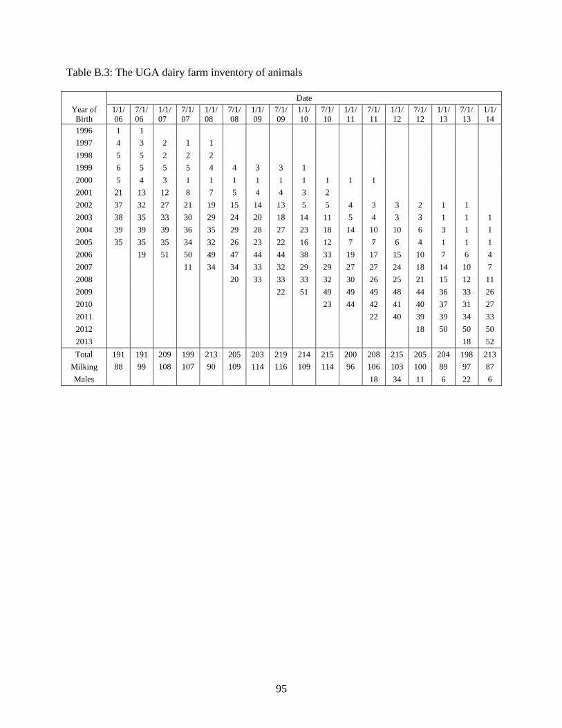
95
Table B.3: The UGA dairy farm inventory of animals
Date
Year of
Birth
1/1/
06
7/1/
06
1/1/
07
7/1/
07
1/1/
08
7/1/
08
1/1/
09
7/1/
09
1/1/
10
7/1/
10
1/1/
11
7/1/
11
1/1/
12
7/1/
12
1/1/
13
7/1/
13
1/1/
14
1996 1 1
1997 4 3 2 1 1
1998 5 5 2 2 2
1999 6 5 5 5 4 4 3 3 1
2000 5 4 3 1 1 1 1 1 1 1 1 1
2001 21 13 12 8 7 5 4 4 3 2
2002 37 32 27 21 19 15 14 13 5 5 4 3 3 2 1 1
2003 38 35 33 30 29 24 20 18 14 11 5 4 3 3 1 1 1
2004 39 39 39 36 35 29 28 27 23 18 14 10 10 6 3 1 1
2005 35 35 35 34 32 26 23 22 16 12 7 7 6 4 1 1 1
2006
19 51 50 49 47 44 44 38 33 19 17 15 10 7 6 4
2007
11 34 34 33 32 29 29 27 27 24 18 14 10 7
2008
20 33 33 33 32 30 26 25 21 15 12 11
2009
22 51 49 49 49 48 44 36 33 26
2010
23 44 42 41 40 37 31 27
2011
22 40 39 39 34 33
2012
18 50 50 50
2013 18 52
Total 191 191 209 199 213 205 203 219 214 215 200 208 215 205 204 198 213
Milking 88 99 108 107 90 109 114 116 109 114 96 106 103 100 89 97 87
Males 18 34 11 6 22 6

96
Table B.4: The UGA dairy farm yearly production in 2013
Test
Date
Days
in
Test
Period
Number
Cows
in Herd
on Test
Day
Test Day
Averages
(Milking
Cows)
Test Day Averages (All
Cows)
Rolling Yearly
Herd Averages
Number
Left Herd Number
Calving
Total
Pregnant
Cows
DIM Milk % in
Milk Milk
%
Fat
%
Protein Milk Fat Protein Died Sold
2-14-13 43 106 198 73.1 88 64.0 4.1 3.1 21,432 859 671 2 5 15 50
3-18-13 32 108 211 67.6 90 60.6 3.7 3.0 21,483 858 673 3 3 12 60
4-16-13 29 110 221 66.5 90 59.8 3.6 3.1 21,452 849 672 0 0 6 66
5-16-13 30 111 229 66.2 90 59.5 3.9 3.1 21,459 844 672 1 3 7 68
6-26-13 41 109 255 55.8 89 49.6 3.6 3.0 21,474 838 673 3 1 3 74
7-25-13 29 108 255 53.0 66 34.9 3.5 2.9 21,399 831 669 0 1 0 76
8-26-13 32 107 282 51.0 63 31.9 3.7 3.0 20,939 811 653 0 1 1 78
9-30-13 35 99 196 59.1 82 48.3 3.8 2.9 20,212 779 628 2 11 37 47
11-5-13 36 102 184 57.3 81 46.5 3.6 3.0 19,777 754 610 2 1 15 42
12-3-13 28 104 162 66.1 79 51.9 3.9 3.0 19,326 732 593 1 4 11 37
1-7-14 35 106 155 68.1 82 55.9 4.1 3.2 18,868 714 577 0 1 14 44
Average 34 106 213 62.2 82 51.2 3.7 3.0 20,711 806 645 14 31 11 58

97
Table B.5: The UGA dairy farm electricity usage
Service Period (days) Usage
(kWh)
Usage per
Day (kWh) Cost ($)
Cost per
Day ($)
9/3/2008 10/2/2008 29 32,238 1,112 3,061.00 105.55
10/2/2008 11/2/2008 31 31,688 1,022 3,139.00 101.26
11/2/2008 12/2/2008 30 36,251 1,208 3,365.00 112.17
12/2/2008 1/4/2009 33 43,175 1,308 3,750.00 113.64
1/4/2009 4/1/2009 29 40,317 1,390 3,548.00 122.34
3/5/2009 3/5/2009 27 28,149 1,043 6,347.00 235.07
2/2/2009 4/1/2009 31 38,349 1,237 3,475.00 112.10
4/1/2009 5/1/2009 30 30,390 1,013 0.00 0.00
5/1/2009 6/2/2009 32
Total for 2009 272 280,557 1,031 26,685
6/2/2009 6/30/2009 28 32,671 1,167 3,101.00 110.75
6/30/2009 7/31/2009 31 36,600 1,181 3,492.00 112.65
7/31/2009 9/1/2009 32 40,101 1,253 3,587.00 112.09
9/1/2009 10/1/2009 30 36,300 1,210 3,395.00 113.17
10/1/2009 10/29/2009 28 25,432 908 2,824.00 100.86
10/29/2009 11/30/2009 32 26,400 825 2,879.00 89.97
11/30/2009 12/30/2009 30 32,438 1,081 3,183.00 106.10
12/30/2009 1/31/2010 32 40,475 1,265 3,656.00 114.25
1/31/2010 3/2/2010 30 33,751 1,125 3,181.00 106.03
3/2/2010 3/31/2010 29 29,387 1,013 3,163.00 109.07
3/31/2010 4/30/2010 30 30,967 1,032 3,286.00 109.53
4/30/2010 4/31/2010 31 34,886 1,125 3,627.00 117.00
Total for 2010 363 399,408 1,100 39,374
5/31/2010 6/29/2010 29 34,927 1,204 3,618.00 124.76
6/29/2010 7/30/2010 31 36,511 1,178 3,590.00 115.81
7/30/2010 8/30/2010 31 38,194 1,232 3,720.00 120.00
8/30/2010 9/29/2010 30 34,950 1,165 3,423.00 114.10
9/29/2010 10/28/2010 29 27,221 939 2,987.00 103.00
10/28/2010 11/30/2010 33 32,406 982 3,264.00 98.91
11/30/2010 1/3/2011 34 38,878 1,143 3,563.00 104.79
1/3/2011 2/1/2011 29 35,900 1,238 3,715.00 128.10
2/1/2011 3/1/2011 28 29,400 1,050 3,343.00 119.39
3/1/2011 3/30/2011 29 33,000 1,138 3,717.00 128.17
3/30/2011 4/30/2011 31 34,377 1,109 3,740.00 120.65

98
Total for 2011 334 375,764 1,125 38,680
4/30/2011 6/3/2011 34 36,273 1,067 3,980.00 117.06
6/3/2011 6/30/2011 27 33,273 1,232 3,918.00 145.11
6/30/2011 7/31/2011 31 38,645 1,247 4,161.00 134.23
Total for 2012 92 108,191 1,176 12,059

99
Table B.6: The UGA dairy farm diesel usage
Purchased
Date Cost ($)
Avrage Price
($/gallon)
Usage
(gallons)
3/31/2012 9,493.93 4.178 2272.63
4/30/2012 5,194.94 4.167 1246.57
5/31/2012 385.06 4.025 95.66
6/27/2012 905.37 3.797 238.44
8/31/2012 1,765.76 3.975 444.24
9/14/2012 584.65 4.109 142.30
10/31/2012 902.00 4.090 220.54
11/30/2012 2,024.36 4.054 499.38
12/21/2012 517.03 4.041 127.95
1/31/2013 427.27 4.008 106.61
2/28/2013 601.53 4.160 144.60
3/29/2013 1,198.21 4.105 291.91
6/28/2013 1,278.29 3.841 332.78
7/30/2013 1,131.18 3.875 291.93
8/30/2013 1,781.10 3.916 454.83
9/30/2013 1,701.32 3.969 428.61
10/30/2013 807.36 3.902 206.94
11/30/2013 1,316.64 3.861 341.01
12/20/2013 296.08 3.919 75.55
2/28/2014 1,551.05 4.116 376.86
3/31/2014 1,711.63 4.132 414.24
4/25/2014 1,434.47 4.070 352.49
5/30/2014 927.55 4.036 229.80
6/30/2014 2,146.26 3.985 538.58
7/31/2014 581.19 3.944 147.35
8/29/2014 741.40 3.881 191.05
9/26/2014 741.40 3.819 194.15
10/31/2014 1,940.54 3.690 525.86
11/30/2014 1,298.90 3.557 365.19
12/23/2014 575.70 3.416 168.53
*Diesel price reference:
http://www.eia.gov/dnav/pet/hist/LeafHandler.ashx?n=PET&s=EMD_EPD2DXL0_PTE_R10_D
PG&f=W