calculating the angular diameter of the sun - stony brook astronomy

On the Calculation of the Angular Diameter

of the Sun by Milchelson Radio Interferometry

Marina von Steinkirch

(laboratory partners: A. Massari and M. von Hippel)

State University of New York at Stony Brook

Department of Physics and Astronomy

Received ; accepted

– 2 –

ABSTRACT

We report the measurement of the angular diameter of the Sun with two

complementary analysis. The observations were perfomed with the Stony Brook

radio interfometer, a compact interferometer that exploits suitable wavelengths

to resolve the magnitudes of the experiment. We measured the total power of

the Sun and of a point source for different distances between the mirrors. We

compare the results of the interfermeter to the simple beam pattern scan. The

fringe pattern by the interferometry data was normalized and Fourier-analyzed.

The peak frequencies were identified and the diameter of the Sun was inferred

from two methods: (i) by Taylor-expanding the visibility function, and (ii) by

fitting the Fourier-transformed sinc visibility function. We verified a value of

ΦTaysun = 37.43′ ± 5.33′ and ΦFit

sun = 32.77′ ± 5.28′, respectively. Both values are

compatibles to the actual value in the literature, ΦActualsun = 31.1′ ± 0.6′.

Subject headings: Radio Interferometry: general — Radio Interferometry: Michelson,

Sun

– 3 –

1. Introduction

In 1921, Michelson and Peace developed the concept of astronomy interferometry (1),

measuring the angular diameter of one the brightness star in the sky, Betelgeuse, with an

optical telescope. Nowadays, Michelson and Peace techniques have broad applications in

astronomy to measure stellar diameters (2).

Optical (wavelength ranges of 390 to 750 nanometers) or Radio interference (wavelength

range of hundreds of meters to millimeters) (3) can be achieved by superimposing signals

from more than one telescope, yielding superior resolutions than that offered by the

telescope alone (4). This is due the fact that the orders of magnitude of the wavelengths in

the radio electromagnetic spectra are scalables to the baselines distances. Interferometry is

a powerful tool in radio astronomy.

A radio interferometer measuring an extensive source such as the Sun will show

a proportional relation of the dimensions of the experiment (i.e., measurable baseline

lengths), to the radio wavelength detected, and to the sizes of fringe, in the resulting power

spectra. In addition, precise values for the baseline lengths can be inferred by observing the

power spectra of a point source (e.g., an artificial geostationary satellite).

In our experiment, we make use of a two-mirrors radio interferometer, assembled in

the Stony Brook University(2), to measure the angular diameter of the Sun, Φsun. We show

that the Sun is roughly resolved when viewed in single-dish mode, but it is well resolved

when observed interferometrically.

– 4 –

1.1. The Geometry of Radio Interferometry

The principle of superposition of waves, figure 1.1, states that when two or more waves

are incident on the same point, the total displacement at that point is equal to the vector

sum of the displacements of the individual waves. If a crest of a wave meets a crest of

another wave of the same frequency at the same point, the magnitude of the displacement

is the sum of the individual magnitudes, yielding a constructive interference. If a crest of

one wave meets a trough of another wave, the magnitude of the displacements equals the

difference in the individual magnitudes, yielding a destructive interference (4).

Fig. 1.— Interference between two plane wave from a distance source at different angles,

from (4). The signals are vectorially added, constructively (a), (c), and destructively (b).

An interferometer will detect and vectorially add signals from two different positions,

figure 2-a. The signal arrives on the two mirrors, being then mixed in the antenna receiver.

The separation between the two positions (mirrors) is named baseline length, B.

– 5 –

Fig. 2.— (left) a - Signal detection on two mirrors on a radio telescope separated by a

baseline length B, from (2). (right) b - Elevation and azimuth angles in the dish.

From an arbitrary origin, we define the horizontal variable angle of the telescope

pointing, θ, and the fixed horizontal angle coordinates of the object in the sky, θ0, as in

figure 2. The angle θ0 will be later related to the actual azimuth, A, of the object. It will

be also useful to calculate the declination, δ of the object (equatorial coordinates), that can

obtained from the elevation, E, the azimuth, and the geographical latitude φ (horizontal

coordinates)(3),

sin δ = sin φ · sin E + cos φ · cos E · cos A. (1)

The signal wavefronts arrive at the telescope in phases because one of the sources

is overhead. The time delay, τ , of the signal at the position 2 (figure 2-a), is related

to difference between these two angles, the baseline length B, and the electromagnetic

radiation speed, c,

τ =B sin(θ − θ0)

c≈ B(θ − θ0)

c, (2)

– 6 –

where we use the fact that θ − θ0 ≪ 1, such that the Taylor-expansion for small-angle

approximation allows sin θ ≈ θ.

1.2. The Physics of Radio Interferometry

Electromagnetic radiation can be written in terms of their perpendicular electric fields,

E, and magnetic fields, B, where the last can be simply derived from the first with the

Maxwell Equations (5).

The radio signal is electromagnetic radiation. At the frequency ν, its time-sinusoidal

amplitude arriving at position 1 (figure 2-a) can be described as a plane wave with the

electric field amplitude (2),

E1(t) = E(θ0) cos[2πνt].

The signal arriving at position 2 at that same time has traveled B sin(θ − θ0) more

than E1(t), and its electric field amplitude is

E2(t) = E(θ0) cos[2πν(t − τ)].

In the interferometer receiver, the two signals are vectorially added,

Etot(t) = E1(t) + E2(t),

and the receiver detects the total power of the signal, P (t). The radio frequency, ν, is large

compared to a data sampling rate of the receiver, and the total power detected is time

averaged (or integrated) (2) (4) (5),

P (t) = 〈Etot(t)2〉,

= E2(θ0)[1 + cos(2πντ)],

P (θ) = E2(θ0)[1 + cos(2πBλ(θ − θ0))], (3)

– 7 –

where Bλ ≡ B/λ, is the normalized baseline length to the wavelength λ = c/ν and we have

applied the results from equation (2).

Considering that the object has an extension in the sky, we can rewrite equation (3) as

a continuum total power law,

P (θ) =

∫

ε(θ0)dθ0

[

1 + cos(

2πBλ(θ − θ0))

]

. (4)

An astronomical object can have any kind of structure, this will result on many kinds

of the energy density distribution, ε(θ0). The telescope interferometer receiver will measure

the sinusoidal power intensity response of the object given by equation (4), where θ are the

fringes pattern due the interferometry. This quantity will be directly related to the Fourier

transformation of the energy density distribution of the object.

1.3. Obtaining the Baseline Lengths from a Point Source

For a punctual source (artificial geostationary satellite), the energy density varying on

θ0 (as we sweep the telescope) is a δ-function at the position of the object:

εsat(θ0) = ε0δ(θ0). (5)

An expect profile of the total power (amplitude squared) of a point source measured

interferometrically can be seen in the figure 3. The pattern of this figure can be thought as

resolved as a serie of point sources, slightly displaced, where the interference and the peaks

and valleys shrink towards the central value of one.

We insert equation (5) into (4) and integrate. As we have mentioned in the beginning

of this session, measurements of a point source yields the accurate measurement of baseline

lengths. The total power is zero in the fringe’s minimums (destructive interference, as

– 8 –

shown in the figure 1.1), becomes

Psat(θ) = ε0

[

1 + cos(

2πBλ(θ − θ0))

]

≡ 0, (6)

meaning

2πBλ(θ − θ0) = (2n + 1)π

Bλ(θ − θ0) =2n + 1

2.

Therefore, the separation between adjacent null positions (i.e., the angular size of the

component we are measuring) gives the value of the baseline lengths,

Bλ∆θ12 =2(n1 − n2)

2,

B∆θλ ≈ 1

∆θ. (7)

(as we can observe, again in the figure 3). We say it is an approximate value because the

rotation of the earth plays a role here, it continuously reorients the telescope, causing the

directions of the constructive/destructive interference to scan across the radio source. For

instance, the earth rotates 0.5o each every 2 minutes. This oscillation/modulation should

be at a much lower frequency than the radio frequency (4).

In addition, with the actual declination of the object, δ, from equation (1), the fringe

∆θ is the Fourier transform of the fringe period ∆t. Considering the angular frequency of

earth rotation as ω = 15o/h, we can also obtain the baseline lengths writing

B∆tλ =

1

cos(δ) sin(ω∆t). (8)

In the rest of this session, we shall write Bλ for simplicity.

– 9 –

Fig. 3.— Example plot of total power as function of telescope pointing, θ for a point source

such as the satellite, from (2).

1.4. Calculating the Angular Diameter of the Sun

We can rewrite the total power given by equation (4),

Psun(θ) =

∫

ε(θ0)dθ0 +

∫

ε(θ0) cos(2πBλ(θ − θ0))dθ0.

This is the the Fourier transformation of the object’s energy density distribution and

we can prove it rewriting the above equation in the same fashion as in (2):

Psun(θ) = Ssun[1 + V (θ, Bλ)],

where

Ssun =

∫

ε(θ0)dθ0,

is the full spectra of the Sun (obtained as a single dish rather than as interferometer), and

V (θ, Bλ) =1

Ssun

∫

ε(θ0) cos[2πBλ(θ − θ0)]dθ0,

= Vsun(Bλ) cos[2πBλθ], (9)

where we gauge the zero-phase position of the coordinates to eliminate a phase. Vsun is the

visibility function of the Sun (an amplitude of the Fourier transform a baseline length Bλ),

Vsun(Bλ) =1

Ssun

∫

ε(θ0)e−i2πBλθ0dθ0. (10)

– 10 –

We can compare this to the observed total power law,

Psun(θ) = Ssun

[

1 + V0(Bλ) cos[2πBλ(θ − ∆θ)]]

.

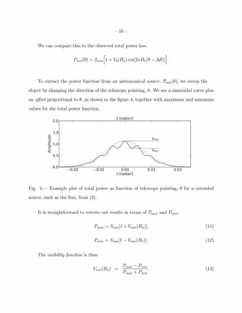
To extract the power function from an astronomical source, Psun(θ), we sweep the

object by changing the direction of the telescope pointing, θ. We see a sinusoidal curve plus

an offset proportional to θ, as shown in the figure 4, together with maximum and minimum

values for the total power function.

Fig. 4.— Example plot of total power as function of telescope pointing, θ for a extended

source, such as the Sun, from (2).

It is straightforward to rewrite out results in terms of Pmax and Pmin,

Pmax = Ssun[1 + Vsun(Bλ)], (11)

Pmin = Ssun[1 − Vsun(Bλ)]. (12)

The visibility function is then

Vsun(Bλ) =Pmax − Pmin

Pmax + Pmin

. (13)

– 11 –

which is a sinc function in term of the baseline lengths,

Vsun(Bλ) =sin(πBλΦsun)

πBλΦsun

,

≡ sinc (BλΦsun). (14)

In this experiment we apply these properties of the visibility function as a Fourier

component of our measurement to obtain the final values of the angular diameter of the

sun.

– 12 –

2. Observations

This experiment is performed with the Stony Brook Michelson Radio Interferometer

(2), during the mornings of February 17th and 26th of 2012. The geographic coordinates of

the site where we were to performed the observations are 40o54′ N 73o08′ W.

The interferometry data was taken only on the second day, from 10 a.m. until 13 p.m

(Eastern Standard Time). The weather was reported as sunny, with temperature around

7oC, and NW winds up to 15 km/h. The altitude and azimuth coordinates of the Sun for

the day of the observation are shown in the appendix, in the table 1.

The Stony Brook’s radio interferometer consists of an electronic part, named Detector,

and a mechanic part, named Radiotelescope, which is further divided ona mount and the

drive.

2.1. The Radiotelescope

The radiotelescope is a dish on a base attached to a frontal ladder. Conceptually it can

subdivided on the following parts (also illustrated in the figure 5):

Siderostat: A central and two lateral mirrored pieces, where the two last have variable

distance lengths (the different baseline lengths in this experiment). The siderostat

combines light onto a single target. The reflective element was building with aluminum

foils (reflectivity of 96% (2)), appropriated to radio observations, e.g., centimeter

wavelengths in this case.

Satellite Dish: Located to be pointed to the target. In the case of the single dish radio

observations, it will be pointed directly to the source (flipped 180o from the mirrors),

i.e., pointing to the opposite side of the siderostats. In the case of the interferometry

– 13 –

observations, the central mirror is faced to the the satellite dish antenna, and this

will vectorially add the electromagnetic signals received from the source by the two

side side mirrors. The broadcast satellite dish operates with frequency/wavelength

ν ∼ 11 GHz, λ ∼ 2.7 cm (2).

Adjustable Baseline Length: A rail designed on a man-hold ladder, where the left and

the right pieces of the siderostat slide, allowing different baseline lengths.

Mount: Driven with motors that electronically adjusts azimuth (left - right) and elevation

(up - down), covering 180 degrees.

Fig. 5.— Pictorial illustration of the Stony Brook’s Michelson-type radio interferometer: the

mirrors can slide through the rail for adjustable baseline lengths. The Central dish stays on

front of the satellite dish antenna.

2.2. The Detection and Analysis Systems

The electronic part of the experiment is composed of commercial receiver amplifier

(satellite finder) and analog-to-digital converter (labpro) connected to a computer (2). The

– 14 –

output is given in voltage (volt) by time (seconds), and acquired in the computer through

the software LoggerPro (8). To convert the observed spectra to power response, we use the

specified Voltage (V) versus Power(dBm) curve, figure 11, in the appendix. The slope is

reported as s = −25(mV/dB), resulting on

PdBm(t) =u(t) V

(−25 mV), (15)

with the conversion of decibel m into a linear power scale is

P (t) = 10PdBm(t)−30

10 . (16)

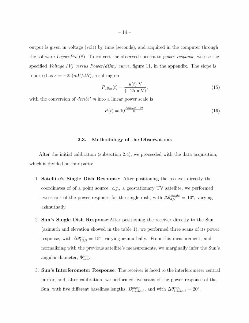
2.3. Methodology of the Observations

After the initial calibration (subsection 2.4), we proceeded with the data acquisition,

which is divided on four parts:

1. Satellite’s Single Dish Response: After positioning the receiver directly the

coordinates of of a point source, e.g., a geostationary TV satellite, we performed

two scans of the power response for the single dish, with ∆θsingle4,5 = 10o, varying

azimuthally.

2. Sun’s Single Dish Response:After positioning the receiver directly to the Sun

(azimuth and elevation showed in the table 1), we performed three scans of its power

response, with ∆θsin1,2,3 = 15o, varying azimuthally. From this measurement, and

normalizing with the previous satellite’s measurements, we marginally infer the Sun’s

angular diameter, ΦSinsun.

3. Sun’s Interferometer Response: The receiver is faced to the interferometer central

mirror, and, after calibration, we performed five scans of the power response of the

Sun, with five different baselines lengths, Bmeas1,2,3,4,5, and with ∆θsun

1,2,3,4,5 = 20o.

– 15 –

4. Satellite Source’s Interferometer Response: We performed five scans of the

power response of the point source, with the same five different baseline lengths,

Bmeas1,2,3,4,5, and with ∆θsat

1,2,3,4,5 = 10o.

2.4. Methodology of the Calibration

The calibration of the radiotelescope was performed in the following way:

Calibrating the azimuth disk and the elevation dial with Sun We need this to

minimize the effect of the telescope aperture attenuation on the measurement of Pmax

and Pmin (equation (13)) when we measure the Sun. In another words, the central

maximum of the interference pattern should be θ = θ0 of the source. With the correct

position of the Sun (table 1) we point the single dish detector directly to it and,

together with an analogical Satellite Finder and the LoggerPro software, we find the

position with highest intensity, scanning vertically. We then trail the elevation dial

to the corrected aligned. We use the latter shadow to align the sun (looking to its

shadow) and the azimuth disk can be calibrated.

Calibrating the Mirrors For the Interferometry observation, we rotate the dish to the

center of the central mirror, with the left and right mirror on their closest position

from the center. We maximize the signal by refining the aim of the telescope. First,

measuring the power for the left mirror alone. Then, performing the measurement

with the right mirror alone. We verifies how the reflected intensities matches.

– 16 –

3. Data Reduction

In this session we discuss how we treat the raw data, which was registered with the

software LoggerPro (8) as measurements of the total output voltage vs time of signal.

3.1. Treatment of the Voltage V(t) Raw Data

To normalize and delogarithm all the four sets of data described in the section 2.3,

we use the equations (15) and (16). The negative slope indicates that the output voltage

decreases as the input power increase. The interferometry results for the Sun and for the

satellite are shown in the figures 6 and 7. The total power is the amplitude squared of the

summed electric vectors of the electromagnetic signals, as we described before.

3.2. The Single Dish Measurements for the Sun and the Satellite

In the single dish mode, the size of the solar disk is the deconvolution of the single dish

solar profile with the single dish satellite profile. We report the single dish profile for one of

the measurements of each of the sources in the figure 8. We use these two profiles to resolve

a first approximation of the solar angular diameter.

– 17 –

50 100 150 200 250 300Time H0.1 sL

2 ´106

4 ´106

6 ´106

8 ´106

1´107

To tal Po we rHmWLSUN-Base line 1

20 40 60 80 100Time H0.1 sL

2 ´106

4 ´106

6 ´106

8 ´106

1´107

PHtL HmWLSUN-Base line 1

50 100 150 200 250Time H0.1 sL

2 ´106

4 ´106

6 ´106

8 ´106

1´107


20 40 60 80 100Time H0.1 sL

2 ´106

4 ´106

6 ´106

8 ´106

1´107


50 100 150 200 250 300Time H0.1 sL

1´106

2 ´106

3 ´106

4 ´106

5´106


20 40 60 80 100Time H0.1 sL

1´106

2 ´106

3 ´106

4 ´106

5´106


50 100 150 200 250 300Time H0.1 sL

1´106

2 ´106

3 ´106

4 ´106

5´106


20 40 60 80 100Time H0.1 sL

1´106

2 ´106

3 ´106

4 ´106

5´106


50 100 150 200 250 300Time H0.1 sL

1´106

2 ´106

3 ´106

4 ´106

5´106


20 40 60 80 100Time H0.1 sL

3.5´106

4.0 ´106

4.5´106

5.0 ´106


Fig. 6.— Interferometer measurements of total power of the Sun, in function of time, for

the five set of measurements. On the right, after the cuts.

– 18 –

20 40 60 80 100 120 140Time H0.1 sL

5.0 ´106

1.0 ´107

1.5´107

To tal Po we rHmWLSATELLITE-Base line 1

10 20 30 40 50Time H0.1 sL

1.3 ´107

1.4 ´107

1.5´107

1.6 ´107

1.7´107

1.8 ´107PHtL HmWL

SAT -Base line 1

20 40 60 80 100 120Time H0.1 sL

5.0 ´106

1.0 ´107

1.5´107


10 20 30 40 50Time H0.1 sL

1.3 ´107

1.4 ´107

1.5´107

1.6 ´107

1.7´107

PHtL HmWLSAT -Base line 2

20 40 60 80 100 120Time H0.1 sL

5.0 ´106

1.0 ´107

1.5´107


10 20 30 40 50Time H0.1 sL

1.3 ´107

1.4 ´107

1.5´107

1.6 ´107

1.7´107


20 40 60 80 100 120Time H0.1 sL

5.0 ´106

1.0 ´107

1.5´107


10 20 30 40 50Time H0.1 sL

1.1´107

1.2 ´107

1.3 ´107

1.4 ´107

1.5´107

1.6 ´107


20 40 60 80 100 120Time H0.1 sL

5.0 ´106

1.0 ´107

1.5´107


10 20 30 40 50Time H0.1 sL

1.1´107

1.2 ´107

1.3 ´107

1.4 ´107

1.5´107


Fig. 7.— Interferometer measurements of total power of the satellite, in function of time,

for the five set of measurements. On the right, after the cuts.

– 19 –

20 40 60 80 100 120Time H0.1 sL

100 000

200 000

300 000

400 000

500 000

600 000

PHtL HmWLSAT Single Dish

10 20 30 40 50 60Time H0.1 sL

100 000

200 000

300 000

400 000

500 000

600 000

PHtL HmWLSAT - Single Dish

20 40 60 80 100 120 140Time H0.1 sL

1´106

2 ´106

3 ´106

4 ´106

PHtL HmWLSUN- Single Dish

10 20 30 40 50 60Time H0.1 sL

1´106

2 ´106

3 ´106

4 ´106


Fig. 8.— Single dish measurements for the Sun and the satellite.

– 20 –

4. Data Analysis and Results

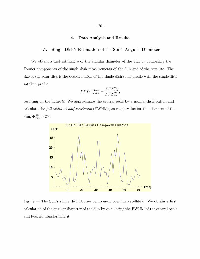
4.1. Single Dish’s Estimation of the Sun’s Angular Diameter

We obtain a first estimative of the angular diameter of the Sun by comparing the

Fourier components of the single dish measurements of the Sun and of the satellite. The

size of the solar disk is the deconvolution of the single-dish solar profile with the single-dish

satellite profile,

FFT (ΦSinsun) =

FFT Sinsun

FFT Sinsat

,

resulting on the figure 9. We approximate the central peak by a normal distribution and

calculate the full width at half maximum (FWHM), as rough value for the diameter of the

Sun, ΦSinsun ≈ 25′.

10 20 30 40 50 60fre q

5

10

15

20

25

FFTSingle Dish Fo urie r Co mpo e nt Sun Sat

Fig. 9.— The Sun’s single dish Fourier component over the satellite’s. We obtain a first

calculation of the angular diameter of the Sun by calculating the FWHM of the central peak

and Fourier transforming it.

– 21 –

4.2. Calculation of the Baselines and Visibility Functions

We calculate the baseline lengths for the set of five measurements of the Sun and

of the satellite with the equation (8), converting the object’s azimuth to the declination

value, as in equation (1). The fringe frequency was numerically calculated by the Fourier

transform profiles of the the total power data. The final values are shown in the table 2 in

the appendix.

From the same Fourier profiles we calculated the Pmax and Pmin points, as shown in

the session 1.4. The visibility functions are automatically obtained from the equation (13).

4.3. Obtaining the Φsun by Taylor-Approximating the Visibility Function

The first method to estimate the value of the diameter of the sun is by plunging the

values we have obtained for the visibility function into a Taylor approximation of the

visibility equation (14),

V Taysun =

sin(x)

x≈ x − x3/6

x= 1 − x2

6

where x = πBλΦTaysun .

This gives a value in radians for the diameter of the Sun for one baseline, and it can

later converted into arc minutes. A Fast Fourier Transform (FFT) of the fringe pattern

shows a peak at the frequency of the fringe period ∆t. Together with the equation (8), the

angular diameter of the Sun can be calculated by

ΦTaysun =

√6

π

1

Bλ

√

1 − V Taysun (Bλ). (17)

The mean and the standard deviation for the five values obtained from this method

results on ΦTaysun = 37.43′ ± 5.33′.

– 22 –

4.4. Obtaining Φsun by Fitting the Fourier Components

The second method to calculate the angular diameter of the sun is based on the fact

that each measurement gives one Fourier component for baseline length. In the observations

we obtain five Fourier components, Vsun(Bλ), which are a Fourier transformation of the

energy density distribution, ε(θ0).

Plotting Vsun(Bλ) vs. Bλ exhibits the Fourier transformation of the object structure.

Since the structure of the Sun should be a top-hat function, the resulting plot (for its

Fourier transformation) is exactly the sinc function,

V fitsun(Bλ) = sinc (BλΦ

fitsun),

we saw in the equation (14). The sinc function sinc(x), also called the sampling function

and arises frequently in signal processing and the theory of Fourier transforms (3).

We plot the Fourier components of the visibility function versus their baseline lengths,

shown in the figure 10. The fit gives the value of ΦFitsun = 32.77′ ± 5.28′.

Sin c Fi t For th e Visb i l i t iy Fu n ct ion sVis ib i l i ty

Basel in e (cm )

200 250 300 350

0.1

0.2

0.3

0.4

120 140 160 180 200Basel in eHcm L

0.1

0.2

0.3

0.4

Visib i l i tySin c Fu n ct ion for Su n

Fig. 10.— The Fourier components of the visibility function versus baselines, which is fitted

by a sinc function, giving the value of the angular diameter of the sun.

– 23 –

4.5. Chi-Squared Fitting

We use our knowledge of the variance (the measure of how far a set of numbers is

spread out) of the measurements to fit it statistically by using the weighted sum of squared

errors:

X2 =∑

i

(Oi − Ei)2

σ2i

.

We assume that the variances, σi, or our measurements are Gaussian functions and

the the above equation will follow a chi-squared distribution. We obtain χ2 = 12.3 for the

previous analysis.

– 24 –

5. Discussion

There were many source of errors in this experiment due to incorrect calibration and

positioning of the sources. The most relevant source of uncertainties, was the incorrect

alignment of the two side mirrors. Due to this fact we see that our profiles are not clean,

most of the times not having a clean central peak.

Despite the high uncertainties, the calculations surprisingly resulted on a good

agreement to the expect value for the diameter of sun in the literature. The second method,

based on the fit of the Fourier components, resulted on a more precise value, as it was

expect. It is not clear how better theses results can be when treating very accurate and

calibrated data instead.

– 25 –

6. Conclusion

Performing two complementary analysis: (i) the Taylor expansion of the visibility

function, and (ii) the fitting of the visibility function, we have found two values for the

angular diameter of the sun, respectively, ΦTaysun = 37.43′ ± 5.33′ and ΦFit

sun = 32.77′ ± 5.28′.

These results are compatibles between themselves and to the value registered in the

literature, ΦActualsun = 31.1′ ± 0.6′ (3).

From the present results we conclude that despite the simple character of the radio

interferometer utilized in this experiment, it shown to be qualified to perform radio

interference at radio wavelengths.

– 26 –

REFERENCES

(1) Albert A. Michelson, Francis G. Pease, Measurement of the diameter of alpha Orionis

with the interferometer, Astrophys. J. 53, 249-259 (1921).

(2) J. Koda & J. Barret, Stony Brook Radio Interferometer, 2012.

(3) http://www.wikipedia.org/ as 03/01/2012.

(4) H. Bradt, Astronomy Methods, Cambridge University Press, 2007.

(5) J. D. Jackson, Classical Electrodynamics, (Third Edition), 1998.

(6) Satellite Finder, http://www.dishpointer.com/, February/2012.

(7) Sun Altitude/Azimuth Table, http://aa.usno.navy.mil/data/docs/AltAz.php,

February/2012.

(8) http://www.vernier.com/products/software/lp.

(10) http://www.wolfram.com/mathematica/.

(9) http://root.cern.ch/drupal/.

– 27 –

Fig. 11.— The convertor from voltage to power.

– 28 –

Table 1. Elevation and Azimuth of the Sun for 02/26/2012 (7)

Eastern Time Elevation Azimuth (E of N)

10:50 37.4 155.2

11:00 38.1 159.3

11:10 38.7 162.3

11:20 39.2 165.4

11:30 39.7 168.6

11:40 40.0 171.8

11:50 40.2 175.0

12:00 40.3 178.2

12:10 40.3 181.5

12:20 40.2 184.7

Note. — The altitude and azimuth of the Sun for

the day of the observations, 02/26/2012, at Stony

Brook University, NY,W 73 08, N40 56.

Table 2. Measured and Calculated Baseline Lengths

Baseline Measured Length (m) Baseline Satellite Length (m) Baseline Sun Length (m)

Bmeas

1 0.60 ± 0.05 Bsat

1 1.40 ± 1.16 Bsun

1 1.01 ± 1.16

Bmeas

2 0.76 ± 0.05 Bsat

2 1.62 ± 1.16 Bsun

2 1.33 ± 1.16

Bmeas

3 0.92 ± 0.05 Bsat

3 1.85 ± 1.16 Bsun

3 1.64 ± 1.16

Bmeas

4 1.08 ± 0.05 Bsat

4 2.16 ± 1.16 Bsun

4 2.02 ± 1.16

Bmeas

5 1.24 ± 0.05 Bsat

5 2.30 ± 1.16 Bsun

5 2.13 ± 1.16

Note. — The first values are the baseline lengths measured from the left border of the left mirror to the

right border of the right mirror. The accurate length measurement should have be done from the middle of

the both mirror. In the final calculations we use the baseline lengths calculated from the analysis, i.e., the

second and third values of the table. The measured values are included for completeness only. Although

the uncertainty for them (which are based on the half of the minimum size of the ruler) are smaller than

for the calculated values, it does not imply that the first values are more precise.

– 29 –

Table 3. Time and Angle Range for the Interferometer Measurements for the Sun

Baseline Label in the Analysis Filename Angle Range in Degrees Eastern Time Sun’s Azimuth

Bsun

1 SUN1 -10,10 1050 155.2

Bsun

2 SUN2 -15,5 1105 162.3

Bsun

3 SUN3 -15,5 1115 165

Bsun

4 SUN41 -15,5 1118 165.4

Bsun

4 SUN42 -10,10 1120 165.4

Bsun

5 SUN5 -10,10 1123 165.4

Note. — Data from the log book. The file SUN42 is the same data than SUN41 so it was not used in the

analysis. We refer to SUN4 instead than SUN41.

Table 4. Time and Angle Range for the Interferometer Measurements for the Satellite

Baseline Label in the Analysis Filename Angle Range in Degrees Eastern Time Satellite’s Azimuth

Bsun

1 SAT1 20,30 1219

Bsun

2 SAT2 20,30 1217

Bsun

3 SAT3 20,30 1215

Bsun

4 SAT4 20,20 1213

Bsun

5 SAT5 20,30 1205

Note. — Data from the log book.

– 30 –

In[611]:= H* MAIN CODE TO FIND THE DIAMETER OF THE SUN BY INTERFEROMETRY*L

m= 5;

H* CONSTANTS*LΩ = 360 Degree H24 *3600L;f = 1000 *10^7;

Λ = 2.99792485*^10 f;

intTime = 100;

vpslope = -25;

suncut = 50;

satcut = suncut 2;

offsetsun = 20;

offsetsat = offsetsun 2;

azimsun = 8155.2, 162.3, 162, 165.4, 165.4 <;∆sun = ArcSin @Sin @-23.44 Degree D*Sin @ azimsun @@mDDDegree DD ;

∆sat = ArcSin @Sin @-23.44 Degree D*Sin @154.1 Degree DD ;

intTime = 100;

timepersweep = 25;

H* OPENING FILES AND CREATING TABLES*LSAT = Import A" homemarina Desktop anaSATSAT" <> ToString @mD<> ".dat", "Table" E;SUN = Import A" homemarina Desktop anaSUNSUN"<> ToString @mD<> ".dat", "Table" E;

H* FIXING POSITIVE VALUES AND FRACTIONAL TIME*LA = Table A8SUN@@i DD@@1DD, Exp @2 - SUN@@i DD@@2DDD<, 9i, 1, Length @SUND=E;B = Table A8SAT@@i DD@@1DD, Exp @2 - SAT@@i DD@@2DDD<, 9i, 1, Length @SATD=E;A1 = Table @0, 81<D;B1 = Table @0, 81<D;

suncurve = Transpose @AD;satcurve = Transpose @BD;

H* CONVERTING FROM VOLT TO TOTAL POWER*Ltimesun = suncurve @@1DD;psun = suncurve @@2DD*H-vpslope L;timesat = satcurve @@1DD;psat = satcurve @@2DD*H-vpslope L;

ListLinePlot Apsun, Background ® LightYellow,

FillingStyle ® Directive AOpacity @0.7 D, LightBlue E,PlotRange ® All, AxesLabel ® 9"Time H0.1 s L", "Total Power HdBmL" =,PlotLabel -> "SUN - Baseline " <> ToString @mD , LabelStyle ® Directive ABold, Medium EE

ListLinePlot Apsat, Background ® LightYellow,

FillingStyle ® Directive AOpacity @0.7 D, LightBlue E,PlotRange ® All, AxesLabel ® 9"Time H0.1 s L", "Total Power HdBmL" =,PlotLabel ® "SATELLITE - Baseline " <> ToString @mD , LabelStyle ® Directive ABold, Medium EE

Printed by Mathematica for Students

Out[638]=

50 100 150 200 250 300Time H0.1 sL

35.0

35.5

36.0

36.5

37.0

To tal Po we rHdBm LSUN -Base line 5

Out[639]=

20 40 60 80 100 120Time H0.1 sL

37

38

39

40

41

42To tal Po we rHdBm L

SATELLITE -Base line 5

In[640]:= H* CONVERTING TOTAL POWER IN dBm TO mW*Lsuncurve = 10^ HHpsun +30L H10LL;satcurve = 10^ HHpsat +30L H10LL;Tsatpow = Table A8j, satcurve @@j DD<, 9j, Length @satcurve D=E;Tsunpow = Table A8j, suncurve @@j DD<, 9j, Length @suncurve D=E;

In[644]:=

In[645]:=

In[646]:= H* CALCULATING PMAX AND PMIN*LMAsun = suncurve;

PPmaxsun = Floor AMedian @Flatten @Position @MAsun, Max@MAsunDDDDE;Pmaxsun = MAsun@@PPmaxsunDD;For Ai = PPmaxsun, i > 20, --i,

If AMAsun@@i - 1DD > MAsun@@i DD,PPminLeftsun = i; Break @D,False

E;E;

For Ai = PPmaxsun, i < Length @MAsunD, ++i,If AMAsun@@i +1DD > MAsun@@i DD,

PPminRightsun = i; Break @D,False

E;E;

Pminsun = MeanA9MAsun@@PPminLeftsun +suncut DD, MAsun AAPPminRightsun +suncut EE=E;

MAsat = satcurve;

PPmaxsat = Floor AMedian @Flatten @Position @MAsat, Max @MAsatDDDDE;

2 diameter_sun.nb


Pmaxsat = MAsat@@PPmaxsat DD;For Ai = PPmaxsat, i > 20, --i,

If AMAsat @@i - 1DD > MAsat@@i DD,PPminLeftsat = i; Break @D,False

E;E;

For Ai = PPmaxsat, i < Length @MAsatD, ++i,If AMAsat@@i +1DD > MAsat@@i DD,

PPminRightsat = i; Break @D,False

E;E;

Pminsat = MeanA9MAsat@@PPminLeftsat +satcut DD, MAsat AAPPminRightsat +satcut EE=E;

cMChecksun = MAsun;

cMChecksun @@PPminLeftsun DD = 0;

cMChecksun AAPPminRightsun EE = 0;

ListLinePlot A9MAsun, cMChecksun =, Background ® LightYellow,

FillingStyle ® Directive AOpacity @0.7 D, LightBlue E,PlotRange ® All, AxesLabel ® 8"Time H0.1 s L", "Total Power HmWL" <,PlotLabel ® "SUN - Baseline " <> ToString @mD , LabelStyle ® Directive ABold, Medium EE

cMChecksat = MAsat;

cMChecksat @@PPminLeftsat DD = 0;

cMChecksat AAPPminRightsat EE = 0;

ListLinePlot A9MAsat, cMChecksat =, Background ® LightYellow,

FillingStyle ® Directive AOpacity @0.7 D, LightBlue E,PlotRange ® All, AxesLabel ® 8"Time H0.1 s L", "Total Power HmWL" <,PlotLabel ® "SATELLITE - Baseline " <> ToString @mD, LabelStyle ® Directive ABold, Medium EE

Out[661]=

50 100 150 200 250 300Time H0.1 sL

1´106

2 ´106

3 ´106

4 ´106

5´106

To tal Po we rHmWLSUN -Base line 5

diameter_sun.nb 3


Out[665]=

20 40 60 80 100 120Time H0.1 sL

5.0 ´106

1.0 ´107

1.5´107

To tal Po we rHmWLSATELLITE -Base line 5

In[666]:= H* CUTTING UNNECESSARY POINTS AND PLOTING*LTsat = Table ATsatpow AAkEE@@2DD, 9k, PPmaxsat - satcut, PPmaxsat +satcut =E;Tsun = Table ATsunpowAAkEE@@2DD, 9 k, PPmaxsun - suncut, PPmaxsun + suncut =E ;

ListPlot Asatcurve, Background ® LightYellow, FillingStyle ® Directive @Opacity @0.7 D, Purple D,Filling ® Axis, AxesLabel ® 8"Time H0.1 s L", "Total Power HmWL" <,PlotLabel ® "SATELLITE - Baseline " <> ToString@mD, LabelStyle ® Directive ABold, Medium EE

ListPlot ATsat, Background ® LightYellow, FillingStyle ® Directive @Opacity @0.7 D, Purple D,Filling ® Axis, AxesLabel ® 8"Time H0.1 s L", " P Ht L HmWL" <,PlotLabel ® "SAT - Baseline " <> ToString @mD, LabelStyle ® Directive ABold, Medium EE

ListPlot Asuncurve, Background ® LightYellow,

FillingStyle ® Directive @Opacity @0.7 D, Purple D, Filling -> Axis,

AxesLabel ® 8"Time H0.1 s L", "Total Power HmWL" <,PlotLabel ® "SUN - Baseline " <> ToString@mD, LabelStyle ® Directive ABold, Medium EE

ListPlot ATsun, Background ® LightYellow,

FillingStyle ® Directive @Opacity @0.7 D, Purple D, Filling -> Axis,

AxesLabel ® 8"Time H0.1 s L", " P Ht L HmWL" <,PlotLabel ® "SUN - Baseline " <> ToString @mD, LabelStyle ® Directive ABold, Medium EE

H* FOURIER TRANSFORMING*LcFFTsun = Abs@Fourier @MAsunDD;cFFTsat = Abs@Fourier @MAsatDD;ListLinePlot AcFFTsun, Background ® LightYellow,

FillingStyle ® Directive AOpacity @0.7 D, LightBlue E, AxesLabel ® 8"Freq", "Fourier Comp" <,PlotLabel ® "SUN - Baseline " <> ToString @mD, LabelStyle ® Directive ABold, Medium EE;

ListPlot AcFFTsun, Background ® LightYellow, FillingStyle ® Directive AOpacity @0.7 D, LightBlue E,Filling ® Axis, AxesLabel ® 8"Freq", "FFT" <,PlotLabel ® "SAT - Baseline " <> ToString @mD, LabelStyle ® Directive ABold, Medium EE;

ListLinePlot AcFFTsat, Background ® LightYellow,

FillingStyle ® Directive AOpacity @0.7 D, LightBlue E, AxesLabel ® 8"Freq", "Fourier Comp" <,PlotLabel ® "SATELLITE - Baseline " <> ToString @mD, LabelStyle ® Directive ABold, Medium EE;

ListPlot AcFFTsat, Background ® LightYellow, FillingStyle ® Directive AOpacity @0.7 D, LightBlue E,Filling ® Axis, AxesLabel ® 8"Freq L", "FFT" <,PlotLabel ® "SAT - Baseline " <> ToString @mD, LabelStyle ® Directive ABold, Medium EE;

4 diameter_sun.nb


Out[668]=

20 40 60 80 100 120Time H0.1 sL

5.0 ´106

1.0 ´107

1.5´107


Out[669]=

10 20 30 40 50Time H0.1 sL

1.1´107

1.2 ´107

1.3 ´107

1.4 ´107

1.5´107


Out[670]=

50 100 150 200 250 300Time H0.1 sL

1´106

2 ´106

3 ´106

4 ´106

5´106


Out[671]=

20 40 60 80 100Time H0.1 sL

3.5´106

4.0 ´106

4.5´106

5.0 ´106


In[678]:=

diameter_sun.nb 5


In[679]:= H* CALCUATING THE BASELINE VALUES in cm*LfringeFreqsun = Flatten APosition ATake AcFFTsun, 9offsetsun, Length @cFFTsun D=E,

MaxATake AcFFTsun, 9offsetsun, Length @cFFTsun D 2 Floor =EEEE@@1DD +offsetsun - 1;

fringeTimesun = 1 IfringeFreqsun ILength @cFFTsun D* timepersweep MM;fringeFreqsat = Flatten APosition ATake AcFFTsat, 9offsetsat, Length @cFFTsat D=E,

MaxATake AcFFTsat, 9offsetsat, Length @cFFTsat D 2 Floor =EEEE@@1DD +offsetsat - 1;

fringeTimesat = 1 IfringeFreqsat ILength @cFFTsat D* timepersweep MM;dCalcsun = Λ HCos@∆sunDSin @Ω * fringeTimesun DLdCalcsat = Λ HCos@∆sat DSin @Ω * fringeTimesat DL

Out[683]= 212.485

Out[684]= 230.083

In[685]:=

In[686]:= H* CALCULATING THE VISIBILITY FUNCTION VALUES *LPPminsat = Floor AMedian @Flatten @Position @MAsat, Min @MAsatDDDDE;Pminsat = MAsun@@PPminsat DD;v = HPmaxsun - Pminsun L HPmaxsun +Pminsun Lvsat = HPmaxsat - Pminsat L HPmaxsat +Pminsat L

Out[688]= 0.23276

Out[689]= 0.493103

In[690]:= H* CALCULATING THE ANGULAR DIAMETER OF THE SUN BY TAYLOR EXPANDING,

UTILIZING THE BASELINES BY THE SUN AND BY THE SAT DATA*LΦ1 = HSqrt @6D Pi L*IΛ dCalcsun M*Sqrt @1 - Abs@vDD;Φ1min = Φ1 *H180 Pi L*60

Φ2 = HSqrt @6D Pi L*IΛ dCalcsat M*Sqrt @1 - Abs@vDD;Φ2min = Φ2 *H180 Pi L*60

Out[691]= 33.1251

Out[693]= 30.5915

6 diameter_sun.nb


In[878]:= H*SINGLE DISH ANALYSIS

*LslopeVP = 25;

Ω = 360 Degree H24 *3600L;Λ = 2.99792485*^8 f;

TSATSIN = Import A" homemarina Desktop anaSINGLESALOLDTXT4.txt", "Table" E;TSUNSIN = Import A" homemarina Desktop anaSINGLESALOLDTXT2.txt", "Table" E;

H* REVERTING NEGATIVE VALUES- THIS IS THE VOLTAGE DATA*LTsatvolt =

Transpose ATable A8TSATSIN@@aDD@@1DD, Exp @2 - TSATSIN@@aDD@@2DDD<, 9a, 2, Length @TSATSIND=EE;Tsunvolt = Transpose ATable A8TSUNSIN@@aDD@@1DD, Exp @2 - TSUNSIN@@aDD@@2DDD<,

9a, 2, Length @TSUNSIND=EE;

H* CONVERTING POWER FROM VOLTAGE*LFsatpow = 10^ HHHTsatvolt @@2DD*slopeVP L+30L H10LL;Fsunpow = 10^ HHHTsunvolt @@2DD*slopeVP L+30L H10LL;

H* NEW TABLE OF POWER SPECTRA*LTsatpow = Table A8j, Fsatpow @@j DD<, 9j, Length @Fsatpow D=E;Tsunpow = Table A8j, Fsunpow @@j DD<, 9j, Length @FsunpowD=E;

H* CALCULATING PMAX AND PMIN AND CENTER*LPsatmaxt = Floor AMedian @Flatten @Position @Fsatpow, Max @Fsatpow DDDDE;Psatmax = Fsatpow @@Psatmaxt DD;For Aj = Psatmaxt, j > 20, --j,

If AFsatpow @@j - 1DD > Fsatpow @@j DD,Psatminleft = j; Break @D,False

E;E;

For Aj = Psatmaxt, j < Length @Tsatpow D, ++j,If AFsatpow @@j +1DD > Fsatpow @@j DD,

Psatminright = j; Break @D,False E

;

E

Psunmaxt = Floor AMedian @Flatten @Position @Fsunpow, Max @FsunpowDDDDE;Psunmax = Fsunpow@@Psunmaxt DD;For Aj = Psunmaxt, j > 20, --j,

If AFsunpow @@j - 1DD > Fsunpow@@j DD,Psunminleft = j; Break @D,False

E;E;

For Aj = Psunmaxt, j < Length @TsunpowD, ++j,If AFsunpow@@j +1DD > Fsunpow@@j DD,


Psunminright = j; Break @D,False

E;E;

Psatmin = MeanA9Fsunpow@@Psatminleft +20DD, Fsunpow AAPsatminright +20EE=E;Psunmin = MeanA9Fsunpow@@Psunminleft +20DD, Fsunpow AAPsunminright +20EE=E;

H* REMOVING UNNECESSARY POINTS*LTsat = Table ATsatpow AAkEE@@2DD, 9k, Psatmaxt - satcut, Psatmaxt + satcut =E;Ffftsat = Abs@Fourier @Tsat DD;ListPlot ATsatpow, Background ® LightYellow, FillingStyle ® Directive AOpacity @0.7 D, Red E,

Filling ® Axis, AxesLabel ® 8"Time H0.1 s L", " P Ht L HmWL" <,PlotLabel ® "SAT Single Dish ", LabelStyle ® Directive ABold, Medium EE

ListPlot ATsat, Background ® LightYellow, FillingStyle ® Directive AOpacity @0.7 D, Red E,Filling ® Axis, AxesLabel ® 8"Time H0.1 s L", " P Ht L HmWL" <,PlotLabel ® "SAT - Single Dish" , LabelStyle ® Directive ABold, Medium EE

Tsun = Table ATsunpowAAkEE@@2DD, 9 k, Psunmaxt - suncut, Psunmaxt + suncut =E ;

Ffftsun = Abs@Fourier @TsunDD;ListPlot ATsunpow, Background ® LightYellow,

FillingStyle ® Directive AOpacity @0.7 D, Red E, Filling -> Axis,

AxesLabel ® 8"freq", " P Ht L HmWL" <, PlotLabel ® "SUN - Single Dish",

LabelStyle ® Directive ABold, Medium EEListPlot ATsun, Background ® LightYellow,

FillingStyle ® Directive AOpacity @0.7 D, Red E, Filling -> Axis,

AxesLabel ® 8"Time H0.1 s L", " P Ht L HmWL" <,PlotLabel ® "SUN - Single Dish", LabelStyle ® Directive ABold, Medium EE

H* CALCULATING FFTSUNFFTSAT *L

Fnorm = Table BFfftsun AAkEEFfftsat AAkEE

, 9k, Length @TsunD=F;

f = Abs@Fourier @FnormDD;ListLinePlot AFnorm, Background ® LightYellow,

FillingStyle ® Directive AOpacity @0.7 D , Red E,AxesLabel ® 8"Time H0.1 s L", " P Ht L HmWL" <,PlotLabel ® "Single Dish Fourier Compoent Sun Sat", LabelStyle ® Directive ABold, Medium EE

2 data_red_single.nb


Out[901]=

20 40 60 80 100 120Time H0.1 sL

100 000

200 000

300 000

400 000

500 000

600 000

PHtL HmWLSAT Single Dish

Out[902]=

10 20 30 40 50 60Time H0.1 sL

100 000

200 000

300 000

400 000

500 000

600 000

PHtL HmWLSAT - Single Dish

Out[905]=

20 40 60 80 100 120 140fre q

1´106

2 ´106

3 ´106

4 ´106


Out[906]=

10 20 30 40 50 60Time H0.1 sL

1´106

2 ´106

3 ´106

4 ´106


data_red_single.nb 3


Out[909]=

10 20 30 40 50 60Time H0.1 sL

5

10

15

20

25

PHtL HmWLSingle Dish Fo urie r Co mpo e nt Sun Sat

In[910]:=

In[911]:=

4 data_red_single.nb


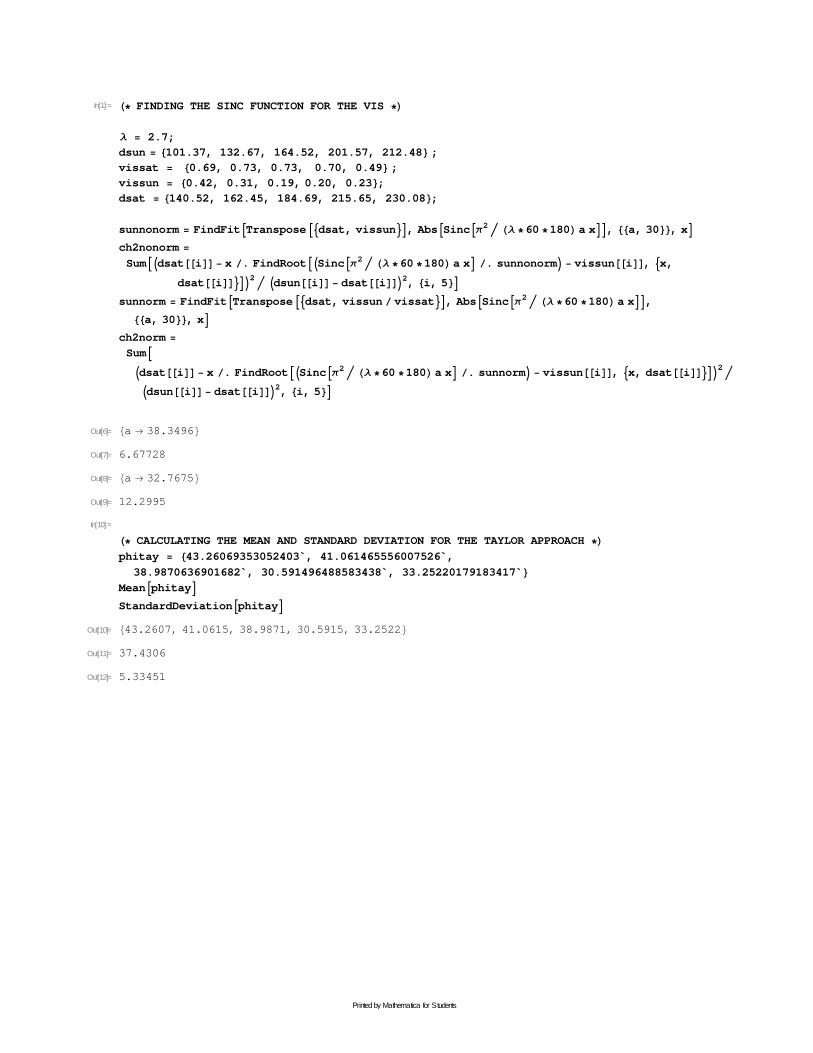
In[1]:= H* FINDING THE SINC FUNCTION FOR THE VIS*L

Λ = 2.7;

dsun = 8101.37, 132.67, 164.52, 201.57, 212.48 < ;

vissat = 80.69, 0.73, 0.73, 0.70, 0.49 < ;

vissun = 80.42, 0.31, 0.19, 0.20, 0.23 <;dsat = 8140.52, 162.45, 184.69, 215.65, 230.08 <;

sunnonorm = FindFit ATranspose A9dsat, vissun =E, Abs ASinc AΠ2 HΛ *60 *180L a xEE, 88a, 30 <<, x Ech2nonorm =

SumAIdsat @@i DD- x . FindRoot AISinc AΠ2 HΛ *60 *180L a xE . sunnonorm M- vissun @@i DD, 9x,

dsat @@i DD=EM2 Idsun @@i DD- dsat @@i DDM2, 8i, 5 <Esunnorm = FindFit ATranspose A9dsat, vissun vissat =E, Abs ASinc AΠ2 HΛ *60 *180L a xEE,88a, 30 <<, x E

ch2norm =

SumAIdsat @@i DD- x . FindRoot AISinc AΠ2 HΛ *60 *180L a xE . sunnorm M- vissun @@i DD, 9x, dsat @@i DD=EM2 Idsun @@i DD- dsat @@i DDM2, 8i, 5 <E

Out[6]= 8a ® 38.3496<

Out[7]= 6.67728

Out[8]= 8a ® 32.7675<

Out[9]= 12.2995

In[10]:=

H* CALCULATING THE MEAN AND STANDARD DEVIATION FOR THE TAYLOR APPROACH*Lphitay = 843.26069353052403`, 41.061465556007526`,

38.9870636901682`, 30.591496488583438`, 33.2522017918 3417` <MeanAphitay EStandardDeviation Aphitay E

Out[10]= 843.2607, 41.0615, 38.9871, 30.5915, 33.2522<

Out[11]= 37.4306

Out[12]= 5.33451


calculating the angular diameter of the sun - stony brook astronomy

Documents