CAE 331/513 Building Science Fall 2013 Lecture 9: November 4, 2013 Cooling loads

Dr. Brent Stephens, Ph.D. Civil, Architectural and Environmental Engineering

Illinois Institute of Technology brent@iit.edu

Advancing energy, environmental, and sustainability research within the built environment www.built-envi.com Twitter: @built_envi

Last time

•  Finished ventilation/infiltration

•  Introduced concepts of heating and cooling loads

•  Performed basic heating load calculations

2

Today’s objectives

•  Finish heating loads –  Latent loads

•  Introduce cooling loads –  Various estimation methods

3

Latent load of humidification

•  How do we account for the energy lost or gained when moist air moves into or out of our building?

•  Textbook example 7.8

4

Cooling loads

5

•  For cooling load calculations things are quite different from heating load calculations

•  Peak cooling loads will be during the day when solar radiation is present

•  Radiation varies during the day and building thermal mass affects radiative heating and cooling –  Calculations must be dynamic

•  People and equipment are usually present and these too can be variable

Dynamic response for cooling loads

•  The cooling load differs from the heat gain because the radiation does not directly heat up the air in the space –  Only convection from interior objects contributes to an immediate

temperature rise in the air space

•  Radiation through windows and from interior surfaces and objects will be absorbed by other interior surfaces and objects, –  Those surfaces will in turn reject that heat to the air by convection,

but the addition of heat doesn’t occur immediately

•  Because radiative heating is not direct, heat storage through thermal mass can create a thermal lag and this can have a large effect on cooling loads

6

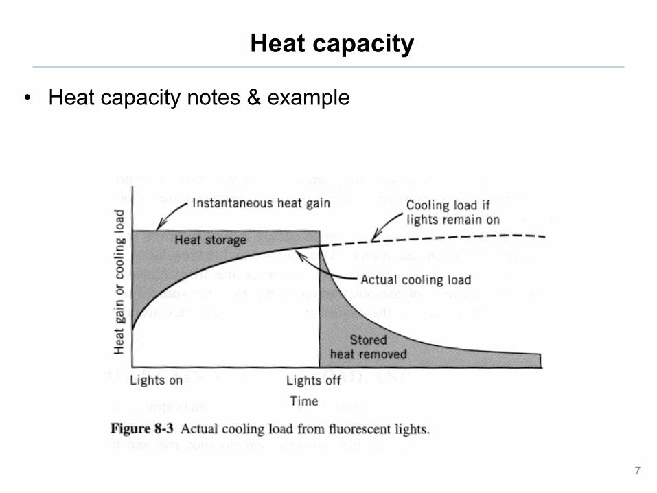
Heat capacity

•  Heat capacity notes & example

7

Cooling load definitions

•  Heat gains = rate at which heat is transferred to or generated in space

•  Cooling load = rate at which cooling equipment would have to remove thermal energy from the air in the space in order to maintain constant temperature/RH

•  Heat extraction rate = rate at which cooling equipment actually does remove thermal energy from the space –  Assumed to equal the cooling load for our purposes

8

Estimating cooling loads

•  Frequently a cooling load must be calculated before every parameter in the conditioned space can be properly or completely defined –  An example is a cooling load estimate for a new building with many

floors of un-leased spaces where detailed partition requirements, furnishings, lighting selection and layout cannot be predefined

–  Potential tenant modifications once the building is occupied also must be considered

•  The total load estimating process requires proper engineering judgment that includes a thorough understanding of heat balance fundamentals

9

Issues with oversizing

10

•  Since getting an accurate cooling load estimate can be difficult (or even impossible at an early design stage) some engineers design conservatively and deliberately oversize systems.

•  Oversizing a system is problematic because –  Oversized systems are less efficient, harder to control, and noisier

than properly sized systems –  Oversized systems tend to duty cycle (turn on and off) which reduces

reliability and increases maintenance costs –  Oversized systems take up more space and cost more

Basic design steps for cooling equipment specification

•  Determine building envelope and owner's criteria •  Determine outside/inside design conditions •  Calculate loads

–  Building loads, heat gains/losses –  System loads, ventilation load, duct leakage

•  Select equipment •  Prepare drawings and specifications

11

Inputs for cooling load calculations

12

Internal and external loads

13

Cooling load calculation methods

•  Transfer Function

•  Total Equivalent Temperature Difference (TETD)

•  Cooling Load Temperature Difference / Cooling Load Factor (CLTD/CLF)

•  Heat Balance Method (HBM)

•  Radiant Time-Series Method (RTSM)

•  They all rely on spreadsheets and/or computer programs 14

Accuracy of methods

15

ASHRAE CLTD/CLF method

•  One method of accounting for periodic responses for conduction and radiation

•  CLTD = cooling load temperature difference [K] –  The temperature difference that gives the same cooling load when

multiplied by UA for a given assembly –  Calculate these delta T values for typical constructions and typical

temperature patterns •  Then adjust the conductive load accordingly

•  CLF = cooling load factor [dimensionless] –  Yields the cooling load at hour t as a function of maximum daily load

•  Also calculated for common construction materials •  Just look values up in tables

16

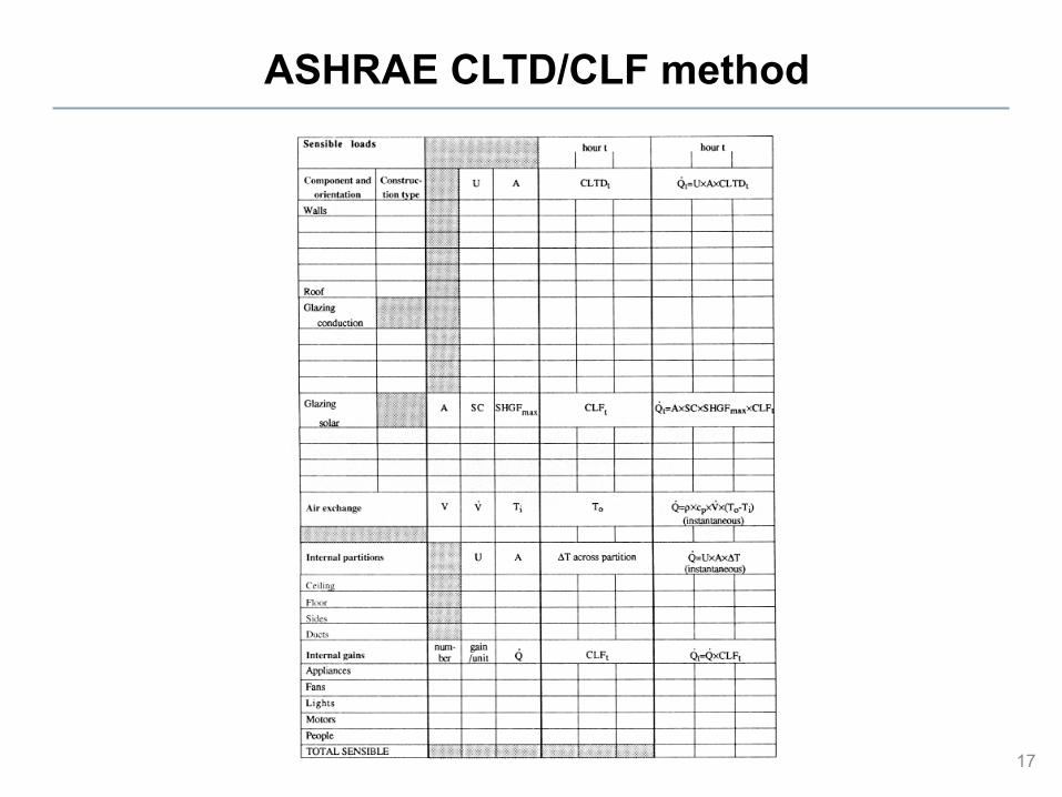
ASHRAE CLTD/CLF method

17

CLTD for roof materials

18

CLTD for wall materials

19 Heavy walls

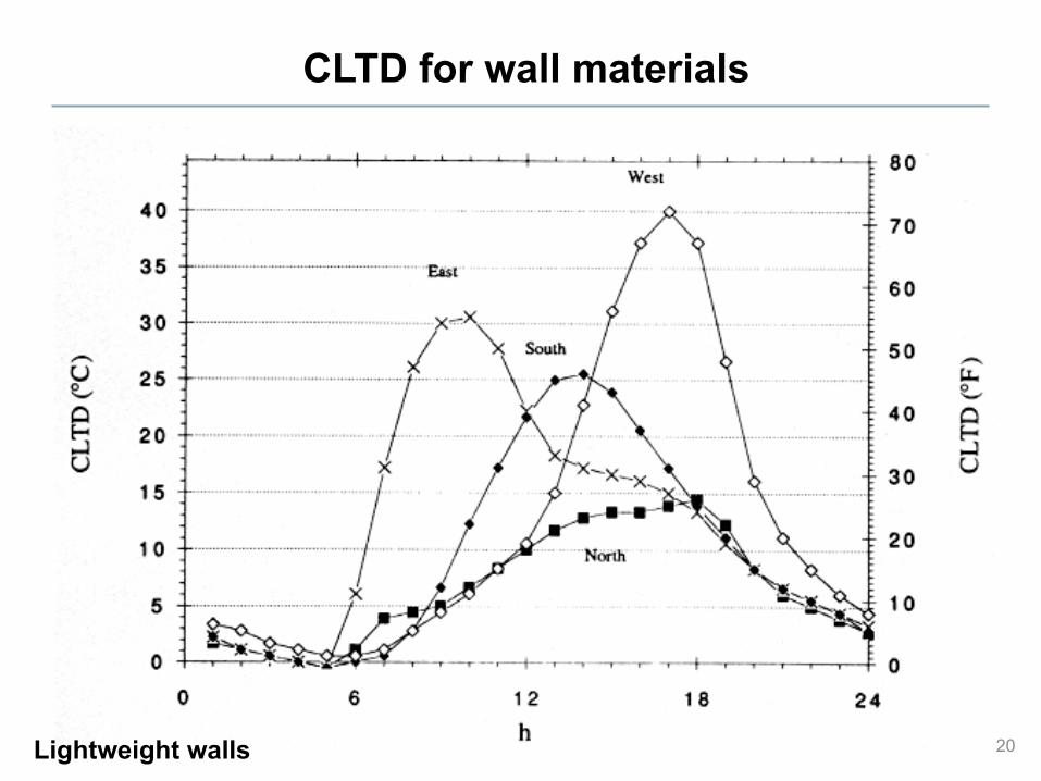
CLTD for wall materials

20 Lightweight walls

CLTD for glass

21

CLF for glass

22

CLF for internal gains

23

Finding peak cooling load with CLTD/CLF method

•  To find the peak cooling load you would need to take into account the magnitude of all individual loads around a peak time period

•  Typically late afternoon or early evening

•  Use a spreadsheet tool

•  This method isn’t used much any more

24

Transfer function method

•  Another more accurate method (but not the most accurate) is the Transfer Function Method

•  Q is a response to driving terms (e.g., Tin, Tout, Qsolar)

•  Assumes: –  Discrete steps –  Linearity –  Causality

•  See notes

25

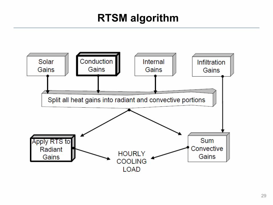
Radiant time-series method (RTSM)

•  The Radiant Time-Series Method (RTSM) is a simplified version of the more complete heat balance version that can be implemented in a spreadsheet or similar software

•  It is suitable for computing fairly accurate peak cooling loads for sizing equipment but not for energy use simulations –  We use the full heat balance method or other methods for that

•  RTSM attempts to include dynamic elements like outdoor air temperatures, solar radiation, and enclosure heat transfer –  Outdoor air temps and solar radiation are cyclic with 24 hour periods –  Enclosure heat capacity will absorb and release heat with a time

delay –  This is like time delays (phase shifts) of electrical networks

26

RTSM simplifying assumptions

•  The combined effects of convective and radiative heat transfer to/from exterior can be modeled by convection to/from an equivalent exterior air temperature called the sol-air temp, Tsol-air –  This means a single combined radiation-convection heat transfer

coefficient independent of wind speed, surface temps and sky temps, must be used for all surfaces

•  All interior surface temperatures are nearly the same so all radiation between elements in the interior can be ignored

27

RTSM main idea

The idea behind the radiant time series is this: •  The current heat transfer to/from the interior is equal to:

+ Part of the current convective heat transfer to the outside of the enclosure

+ current solar heat gain through fenestration + part of the earlier convective and radiative heat transfer to the outside of the enclosure

28

RTSM algorithm

29

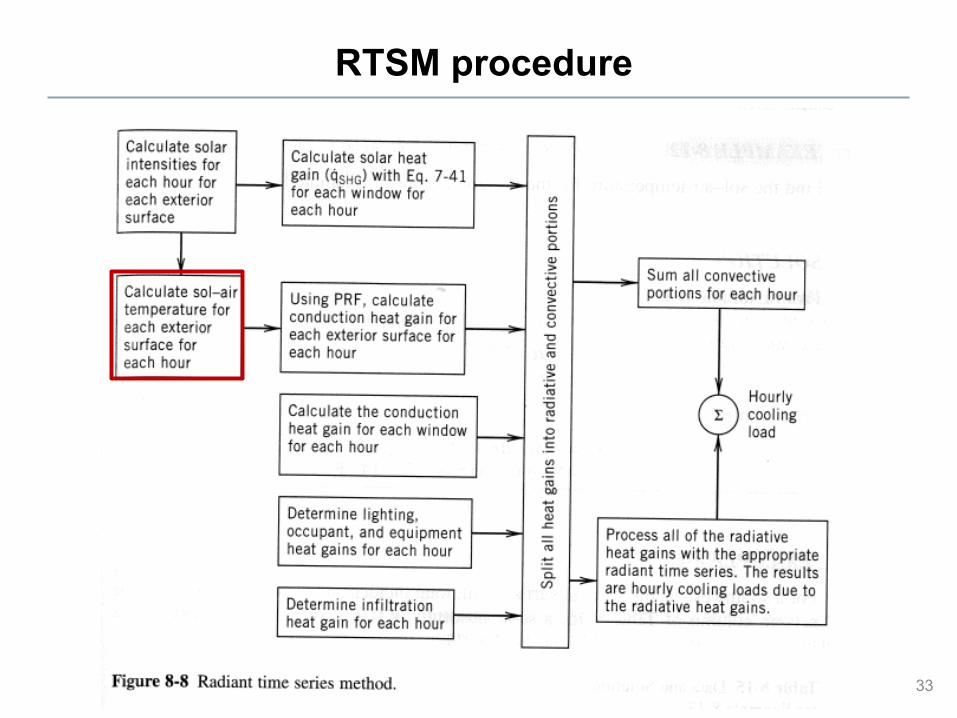
RTSM procedure

30

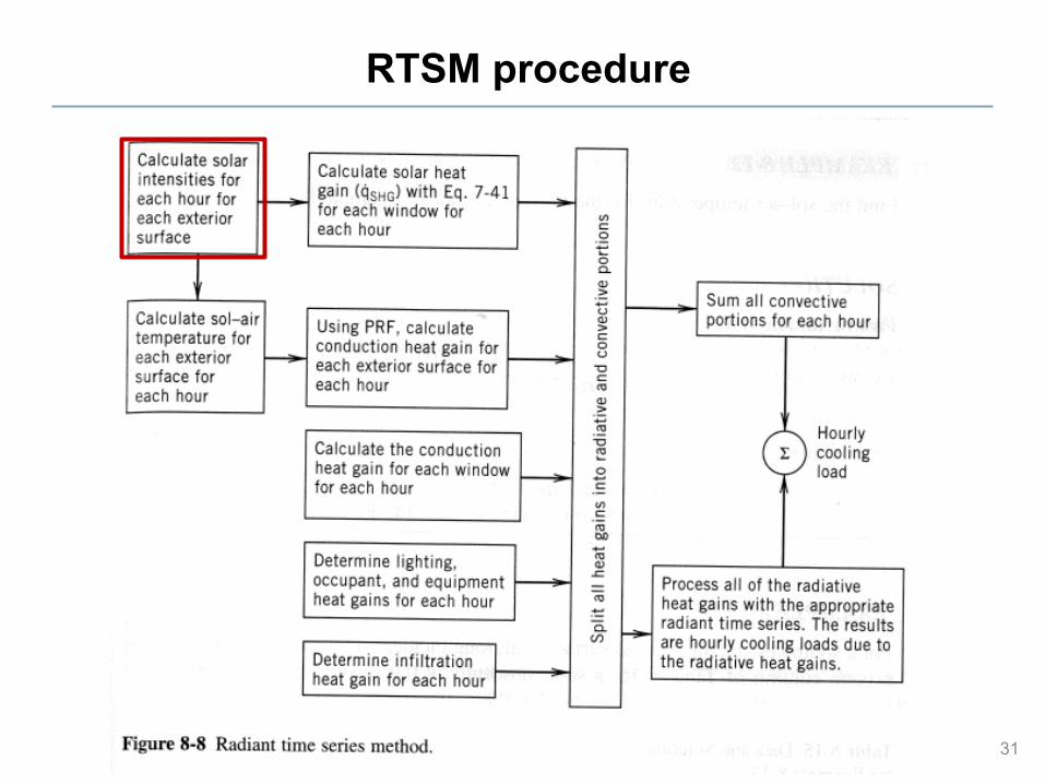
RTSM procedure

31

Solar intensities

•  We can calculate hourly solar intensities based on solar geometry

•  Or download data from the internet –  http://rredc.nrel.gov/solar/old_data/nsrdb/

•  This is often given to us

32

RTSM procedure

33

Calculate sol-air temperature

•  For each surface •  For each hour

•  Table 8-15 in McQuiston et al.

34

Tsol!air =Tair ,out +!Isolar

hext ,conv+rad!!

"Rhext ,conv+rad

!"R ! 7°F for horizontal surfaces!"R ! 0°F for vertical surfaces

RTSM procedure

35

Solar heat gain through windows

•  Each window •  Each hour

•  We’ve done this before

36

qwindow =Upf Tout !Tin( )+ IdirectSHGC(! )IAC(! ,")+ (Idiffuse+reflected )SHGCdiffuse+reflected IACdiffuse+reflected

RTSM procedure

37

Conduction heat gains and “PRF”

•  Heat gains to the interior from conduction will be a sum of conduction going on right now + part of the heat transferred to the enclosure at earlier times

•  For example: q(n)=C0U(Te(n) - Ti(n)) + C1U(Te(n-1) - Ti(n-1)) + … + C23U(Te(n-23) - Ti(n-23))

where Te = Tsol-air

•  We call Cn the conduction time series

•  Ypn =Cn U is the periodic response factor (PRF) in [W/m2K]

38

Conduction heat gains and “PRF”

•  Once we have Ypn we can write the heat conduction into the room at the current time

39

qconduction,in,t = Ypnn=0

23

! Te,q!n !Trc( ) [Btu/(h ! ft2) or W/m2]

where Te,q!n=the sol-air temp n hours ago

Trc= constant interior room temp

Ypn =periodic response function

Using Ypn

40

•  To use the previous equation we need to know the sol-air temp for the previous 24 hours

•  The calculation for 8am would look like this:

qconduction,in,8am =Yp0 Te,8am !Trc( )+Yp1 Te,7am !Trc( )+Yp2 Te,6am !Trc( )+Yp3 Te,5am !Trc( )+Yp4 Te,4am !Trc( )+Yp5 Te,3am !Trc( )+!+Yp22 Te,11am !Trc( )+Yp23 Te,10am !Trc( )+Yp24 Te,9am !Trc( )

The underlined times are from the day before!

Finding Ypn and Cn

•  Ypn depends highly on the exact details of the enclosure construction (wall or ceiling) –  Overall insulation, mass, heat capacity and the insulation location

both are important –  The ASHRAE handbook has a table of U and Cn values for 20

common constructions

41

Example Ypn

42

•  Type 20: Brick + 8” concrete + R11 insulation + gyp board •  Type 3: 1” stone + R10 insulation + gyp board

Also see Table 8-18 in McQuiston et al.

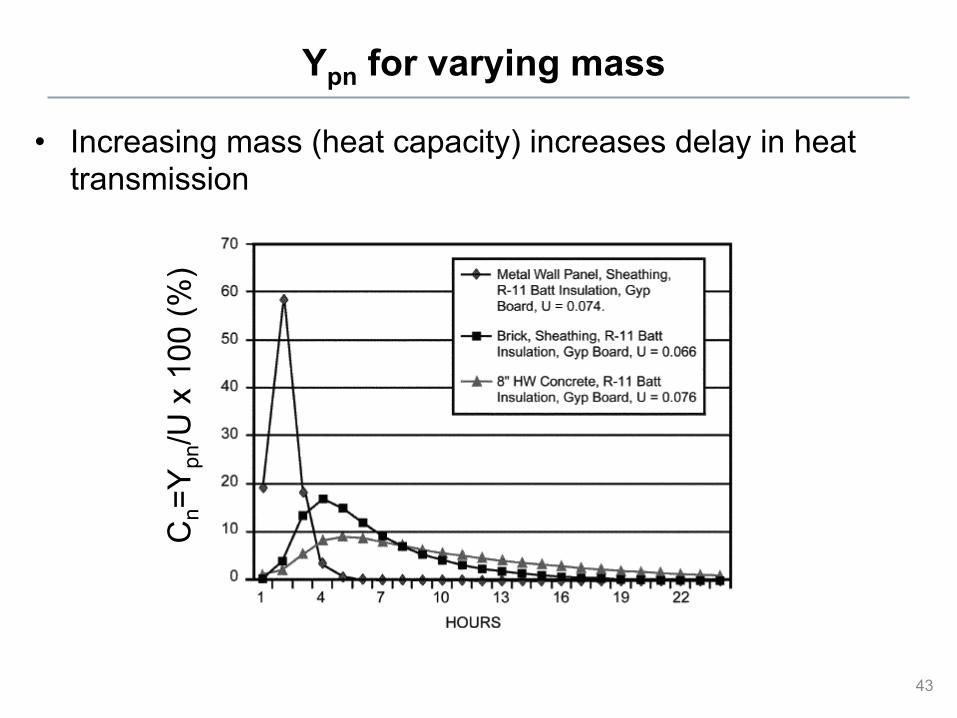
Ypn for varying mass

•  Increasing mass (heat capacity) increases delay in heat transmission

43

Cn=

Ypn

/U x

100

(%)

Ypn for varying insulation

•  Increasing Interior insulation increases delay but increasing exterior insulation does not

44

Cn=

Ypn

/U x

100

(%)

RTSM procedure

45

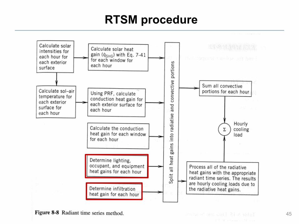
Infiltration and internal gains

•  We treat infiltration gains as instantaneous gains –  We’ve already done this –  We calculate these separately for each hour of the day because the

exterior air temperature changes each hour

•  We calculate internal gains using methods discussed earlier –  We calculate these each hour too because the internal loads will

change from hour to hour –  Also need to keep track of the radiative + convective parts

46

Splitting gains into radiative and convective portions

•  At each hour, each heat gain must be split into radiative parts + convective parts –  “Delayed” versus “instantaneous”

47

Application of the RTSM

•  Convection is considered instantaneous

•  Radiation estimates cooling load due to the radiative portion of each heat gain by applying a radiant time series –  This is analogous to the periodic response factors (PRF) for

conduction based on current and past values of sol-air temperatures

•  Radiant energy is absorbed + reradiated + absorbed + reradiated + absorbed + … –  We must add up portions of radiation from previous hours to find the

total radiant contribution now (kind of like we did with conduction)

48

Total radiant contribution

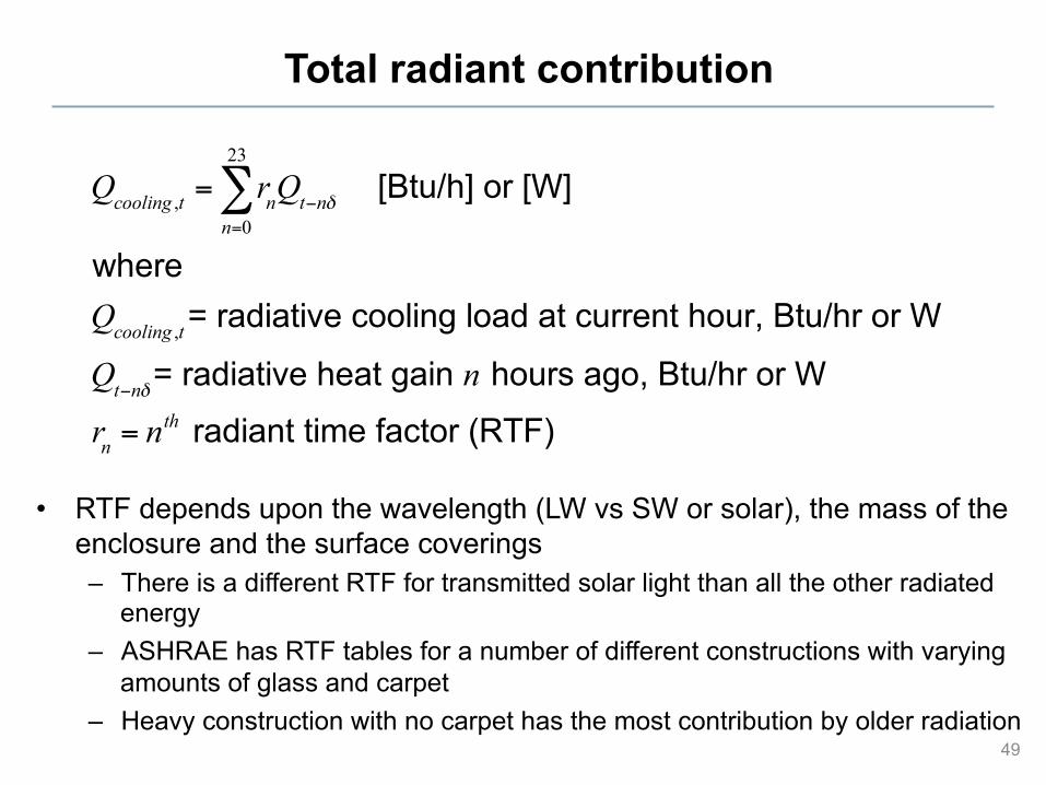
•  RTF depends upon the wavelength (LW vs SW or solar), the mass of the enclosure and the surface coverings –  There is a different RTF for transmitted solar light than all the other radiated

energy –  ASHRAE has RTF tables for a number of different constructions with varying

amounts of glass and carpet –  Heavy construction with no carpet has the most contribution by older radiation

49

Qcooling ,t = rnQt!n!n=0

23

! [Btu/h] or [W]

where Qcooling ,t= radiative cooling load at current hour, Btu/hr or W

Qt!n!= radiative heat gain n hours ago, Btu/hr or W

rn = nth radiant time factor (RTF)

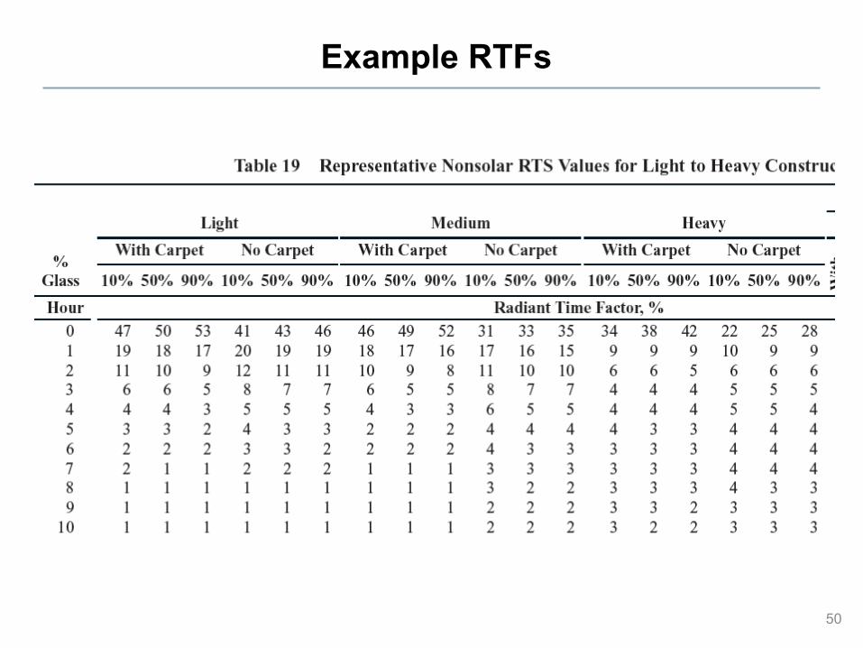
Example RTFs

50

RTSM example

•  Outdoor conditions –  Montreal –  July 21 –  83F dry bulb

•  17.6F daily range –  Ground reflectivity = 0.2

•  Indoor conditions –  Air temperature = 72F

51

•  Other heat gains –  10 occupants –  1 W/ft2 equipment gain

8AM to 5 PM •  0.2 W/ft2 5P-8A

–  1.5 W/ft2 lighting gain 8AM to 5 PM

•  0.3 W/ft2 5P-8A

–  Ignore infiltration

•  Assume only S wall and roof are exposed to outside

•  Wall is 280 ft2, α=0.9 •  Roof is 900 ft2, α=0.9 •  Ypn as shown in the

spreadsheet

•  80 ft2 of window on S wall •  No shading •  SHGC=0.76, U=0.55

You would create a spreadsheet

52

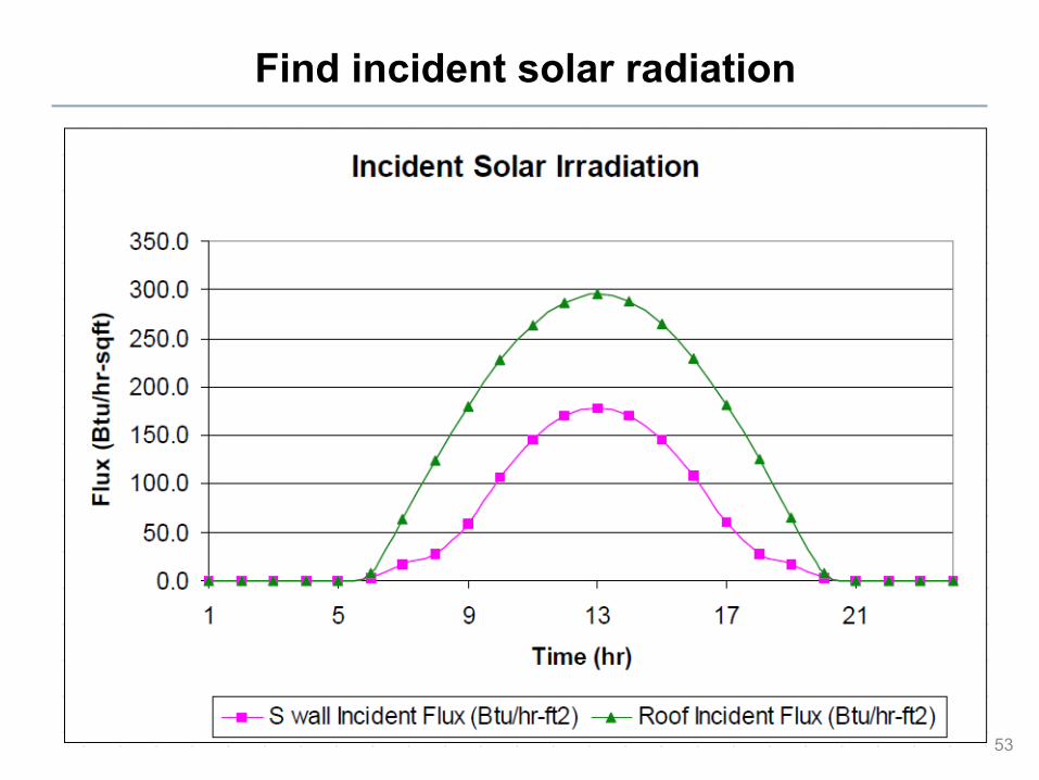
Find incident solar radiation

53

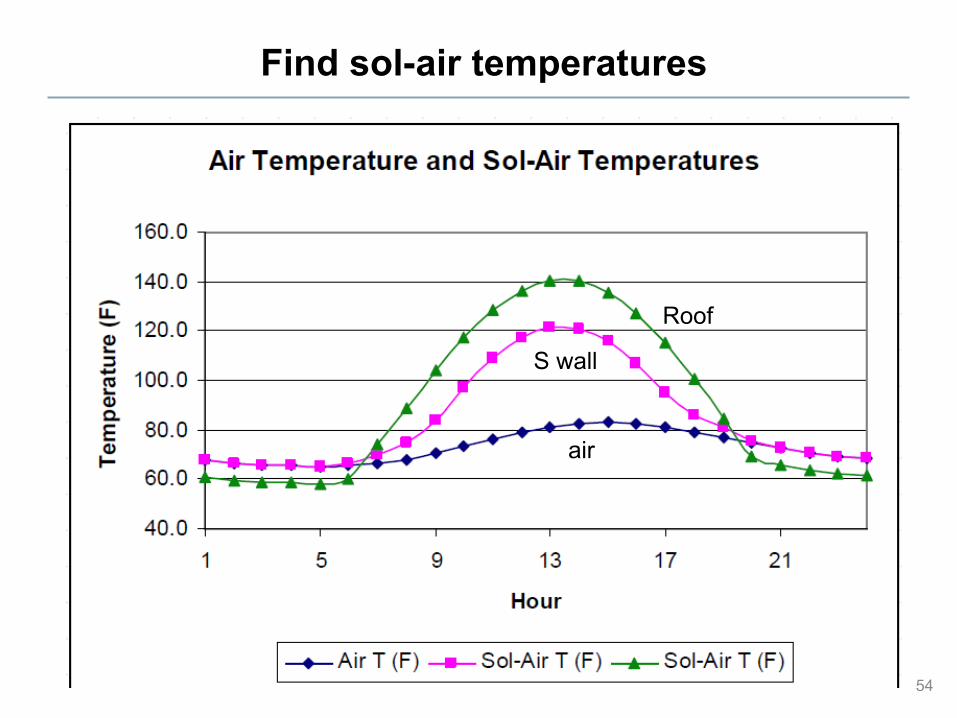
Find sol-air temperatures

54

Roof

S wall

air

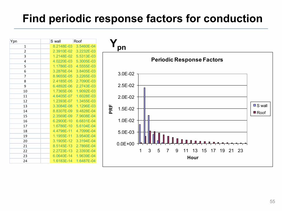
Find periodic response factors for conduction

55

Ypn

0.0E+00

5.0E-03

1.0E-02

1.5E-02

2.0E-02

2.5E-02

3.0E-02

1 3 5 7 9 11 13 15 17 19 21 23

PRF

Hour

Periodic Response Factors

S wall

Roof

Ypn S wall Roof1 8.2148E-03 3.5460E-042 2.3910E-02 3.2232E-033 1.2148E-02 5.5313E-034 4.0220E-03 5.3005E-035 1.1786E-03 4.5555E-036 3.2876E-04 3.8405E-037 8.9655E-05 3.2265E-038 2.4185E-05 2.7090E-039 6.4892E-06 2.2743E-0310 1.7365E-06 1.9092E-0311 4.6405E-07 1.6028E-0312 1.2393E-07 1.3455E-0313 3.3084E-08 1.1296E-0314 8.8307E-09 9.4828E-0415 2.3569E-09 7.9608E-0416 6.2900E-10 6.6831E-0417 1.6786E-10 5.6104E-0418 4.4798E-11 4.7099E-0419 1.1955E-11 3.9540E-0420 3.1905E-12 3.3194E-0421 8.5145E-13 2.7866E-0422 2.2723E-13 2.3393E-0423 6.0640E-14 1.9639E-0424 1.6183E-14 1.6487E-04

Estimate hourly conductive heat gains

56

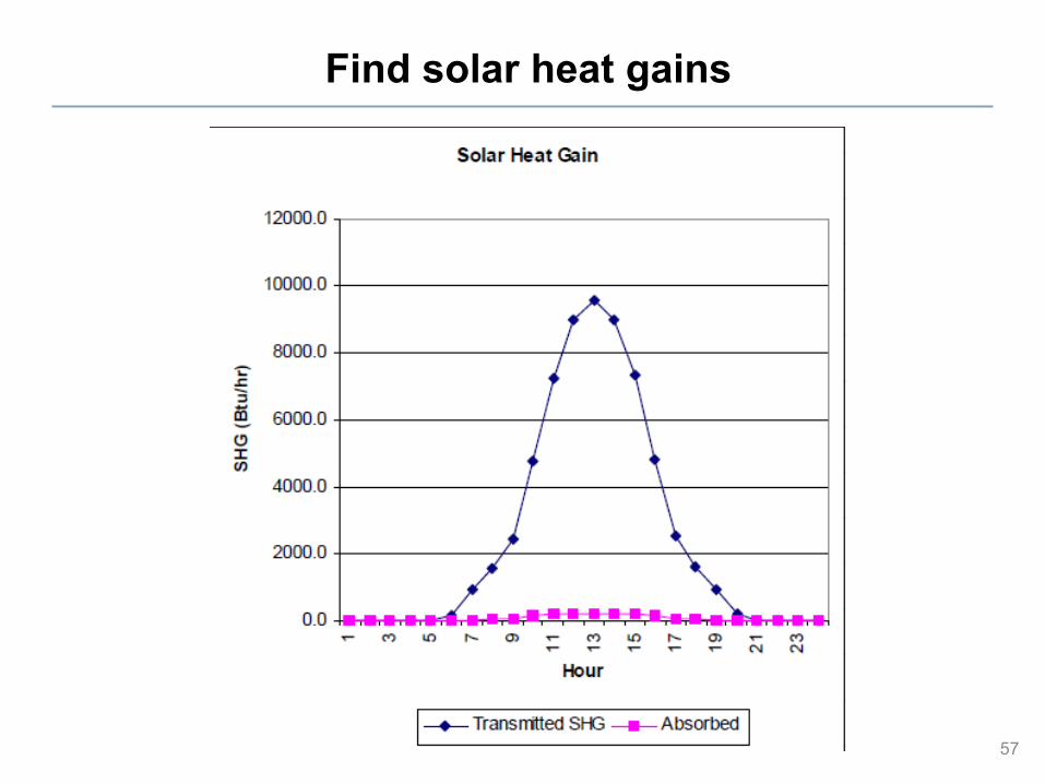
Find solar heat gains

57

Radiative vs. convective split gains

58

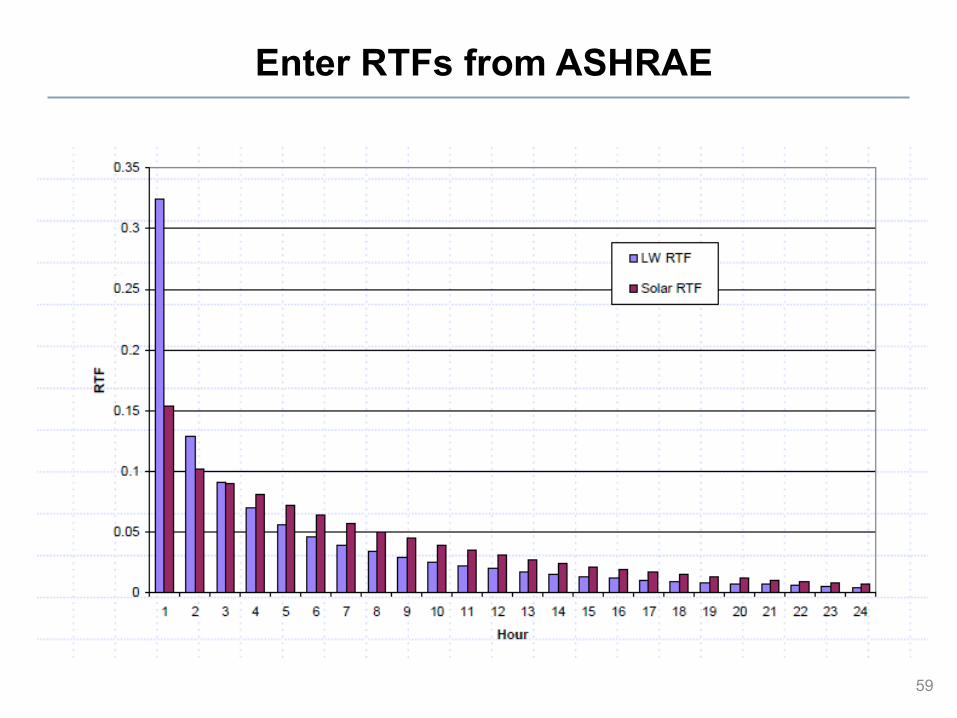
Enter RTFs from ASHRAE

59

Sum all to get total hourly cooling loads

60

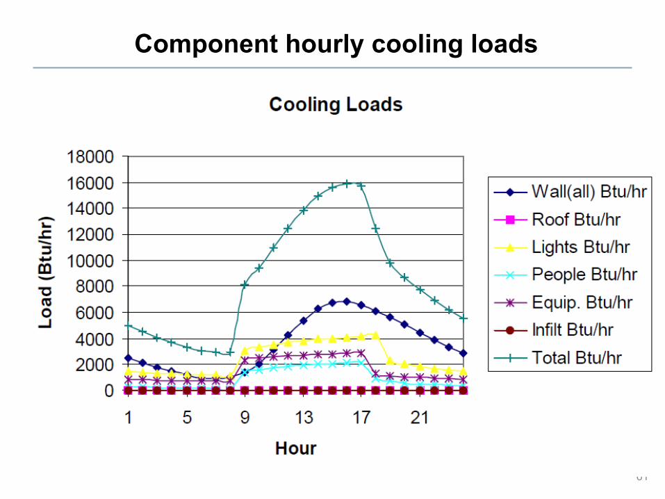
Component hourly cooling loads

61

Another RTSM example

•  ASHRAE Handbook RTS example…

62

Software tools for load calcs

•  These are not done by hand, sometimes by spreadsheet –  Many use ACCA Manual J

•  Most use computer programs

•  Big list of programs: –  http://apps1.eere.energy.gov/buildings/tools_directory/subjects.cfm/

pagename=subjects/pagename_menu=whole_building_analysis/pagename_submenu=load_calculation

63

Last: Heat balance method

•  Let’s also describe the basics behind the heat balance method

•  Relies on a combination of surface and air energy balances

•  Requires a computer program

•  Foundation of modern energy simulation programs –  We cover this in 463/524 Building Enclosure Design

64

Surface energy balance

65

•  Exterior surface example: roof Once you have this equation described, you can do just about anything regarding heat transfer in building enclosure analysis, leading into full-scale energy modeling

qsolar + qlongwaveradiation + qconvection ! qconduction = 0

Steady-state energy balance at this exterior surface: What enters must also leave (no storage)

Surface energy balance

66

•  Exterior surface example: roof

qsw,solar+qlw,surface!sky+qlw,surface!air+qconvection!qconduction = 0

!Isolar+"surface#Fsky (Tsky

4 !Tsurf4 )

+"surface#Fair (Tair4 !Tsurface

4 )+hconv (Tair !Tsurface )!U(Tsurface !Tsurface,interior ) = 0

Solar gain

Surface-sky radiation

Surface-air radiation

Convection on external wall

Conduction through wall

q! = 0

We can use this equation to estimate indoor and outdoor surface temperatures At steady state, net energy balance is zero •  Because of T4 term, often requires

iteration

Surface energy balance

•  Similarly, for a vertical surface:

67

qsolar + qlwr + qconv ! qcond = 0

!Isolar+"surface#Fsky (Tsky

4 !Tsurf4 )

+"surface#Fair (Tair4 !Tsurface

4 )+hconv (Tair !Tsurface )!U(Tsurface !Tsurface,interior ) = 0

Ground

!Isolar+"surface#Fsky (Tsky

4 !Tsurface,ext4 )

+"surface#Fair (Tair4 !Tsurface,ext

4 )+"surface#Fground (Tground

4 !Tsurface,ext4 )

+hconv (Tair !Tsurface,ext )!U(Tsurface,ext !Tsurface,int ) = 0

Combining surface energy balances

•  For an example room like this, you would setup a system of equations where the temperature at each node (either a surface or within a material) is unknown –  12 material nodes + 1 indoor air node

68

Room

F

C

L R

1

1

11

2

2

22

3

3

33

A air node

internal surface node

external surface nodeelement-inner node

Con

vect

ion

Rad iati onmcpdTdt

= qat boundaries!

At surface nodes: q! = 0

At nodes inside materials:

Based on density and heat capacity of material…

Heat Xfer @ external surfaces: Radiation and convection

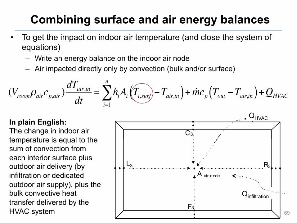
Combining surface and air energy balances •  To get the impact on indoor air temperature (and close the system of

equations) –  Write an energy balance on the indoor air node –  Air impacted directly only by convection (bulk and/or surface)

69

(Vroom!aircp,air )dTair,indt

= hiAi Ti,surf !Tair,in( )i=1

n

" + !mcp Tout !Tair,in( )+QHVAC

F

C

L R

3

3

33

A air node

EiQHVAC In plain English:

The change in indoor air temperature is equal to the sum of convection from each interior surface plus outdoor air delivery (by infiltration or dedicated outdoor air supply), plus the bulk convective heat transfer delivered by the HVAC system

Qinfiltration

Energy simulation

•  Energy 2D

70

FLUID FLOWS In buildings

71

Fluid flows in buildings

•  We use liquids and gases to deliver heating or cooling energy in building mechanical systems –  Water, refrigerants, and air

•  We often need to understand fluid motion, pressure loses, and pressure rises by pumps and fans in order to size systems

•  We can use the Bernoulli equation to describe fluid flows in HVAC systems

72

p1 +12!1v1

2 + !1gh1 = p2 +12!2v2

2 + !2gh2 +Kv2

2Static

pressure Velocity pressure

Pressure head Friction

Pressure losses

•  We often need to find the pressure drop in pipes and ducts •  Most flows in HVAC systems are turbulent

73

!p friction = fLDh

"

#$

%

&'12!v2

"

#$

%

&'

Dh =4AP= hydraulic diameter

K = f LDh

!

"#

$

%& In a straight pipe

K = f LDh

+ K ffittings!

"

#$$

%

&'' In a straight pipe with fittings

Friction factor

74

Reynolds number

•  Reynolds number relates inertial forces to viscous forces:

•  Kinematic viscosity

75

! =µ"=1.5!10"5 m2

s (for air at T=25!C)

Re = VL!

L = Dh in a pipe or duct

Pressure losses and rises

76

Energy input into system by fan

Supply side: Positive pressure

Return side: Negative pressure

Duct friction charts

77

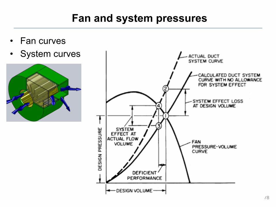
Fan and system pressures

•  Fan curves •  System curves

78

Fan and system curves: Ideal

79

Wfan =!P " !V! fan

Fan and system curves: Real

80

Wfan =!P " !V! fan