CADE: Detecting and Explaining Concept Drift Samplesfor Security Applications

Limin Yang*, Wenbo Guo†, Qingying Hao*, Arridhana Ciptadi‡

Ali Ahmadzadeh‡, Xinyu Xing†, Gang Wang*

*University of Illinois at Urbana-Champaign †The Pennsylvania State University ‡Blue Hexagonliminy2@illinois.edu, wzg13@ist.psu.edu, qhao2@illinois.edu, {arri, ali}@bluehexagon.ai, xxing@ist.psu.edu, gangw@illinois.edu

AbstractConcept drift poses a critical challenge to deploy machinelearning models to solve practical security problems. Dueto the dynamic behavior changes of attackers (and/or thebenign counterparts), the testing data distribution is oftenshifting from the original training data over time, causingmajor failures to the deployed model.

To combat concept drift, we present a novel system CADEaiming to 1) detect drifting samples that deviate from existingclasses, and 2) provide explanations to reason the detecteddrift. Unlike traditional approaches (that require a large num-ber of new labels to determine concept drift statistically), weaim to identify individual drifting samples as they arrive. Rec-ognizing the challenges introduced by the high-dimensionaloutlier space, we propose to map the data samples into alow-dimensional space and automatically learn a distancefunction to measure the dissimilarity between samples. Usingcontrastive learning, we can take full advantage of existinglabels in the training dataset to learn how to compare andcontrast pairs of samples. To reason the meaning of the de-tected drift, we develop a distance-based explanation method.We show that explaining “distance” is much more effectivethan traditional methods that focus on explaining a “decisionboundary” in this problem context. We evaluate CADE withtwo case studies: Android malware classification and networkintrusion detection. We further work with a security com-pany to test CADE on its malware database. Our results showthat CADE can effectively detect drifting samples and providesemantically meaningful explanations.

1 Introduction

Deploying machine learning based security applications canbe very challenging due to concept drift. Whether it is mal-ware classification, intrusion detection, or online abuse detec-tion [6, 12, 17, 42, 48], learning-based models work under a“closed-world” assumption, expecting the testing data distribu-tion to roughly match that of the training data. However, the

Training DataOriginal Classifier

Incoming Samples...

labels

Attack-2

Attack-1

Benign

1 2

0

Detect Drifting Explain Drifting

Production

Space

Monitoring

Space

“Interpretation”

Facilitate Model Update

CADE

Figure 1: Drifting sample detection and explanation.

environments in which the models are deployed are usuallydynamically changing over time. Such changes may includeboth organic behavior changes of benign players and mali-cious mutations and adaptations of attackers. As a result, thetesting data distribution is shifting from the original trainingdata, which can cause serious failures to the models [23].

To address concept drift, most learning-based models re-quire periodical re-training [36, 39, 52]. However, retrainingoften needs labeling a large number of new samples (expen-sive). More importantly, it is also difficult to determine whenthe model should be retrained. Delayed retraining can leavethe outdated model vulnerable to new attacks.

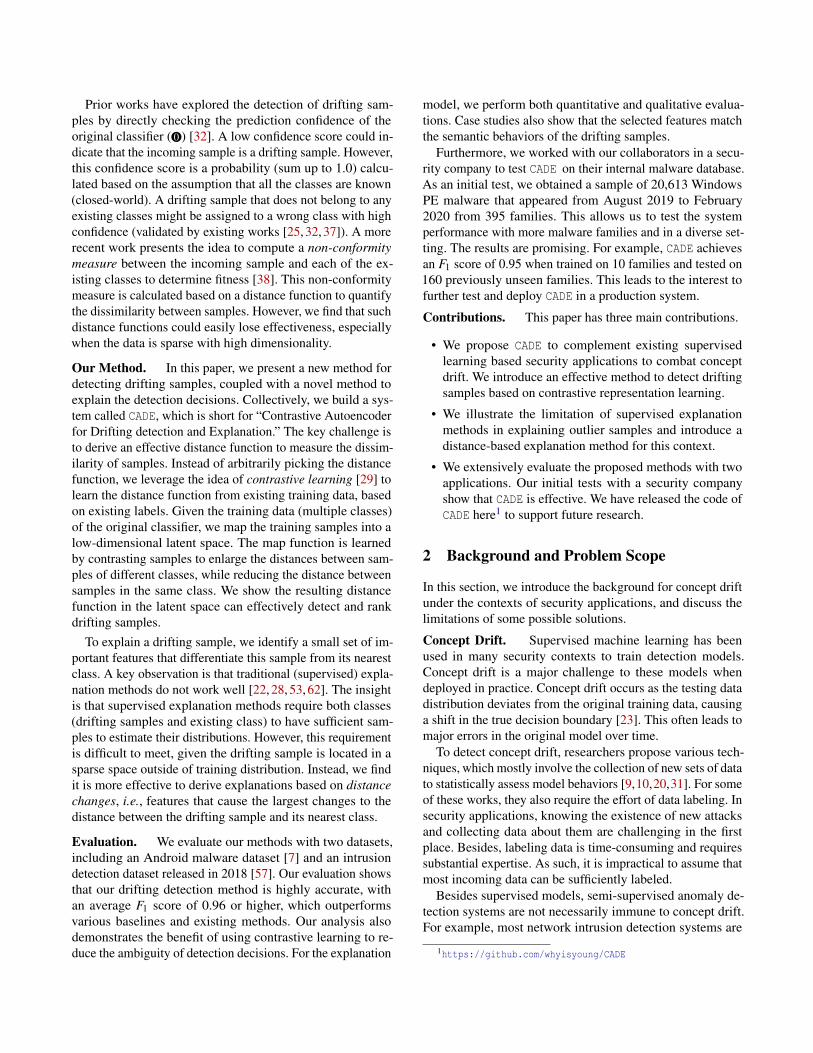
We envision that combating concept drift requires estab-lishing a monitoring system to examine the relationship be-tween the incoming data streams and the training data (and/orthe current classifier). The high-level idea is illustrated inFigure 1. While the original classifier is working in the pro-duction space, another system should periodically check howqualified the classifier is to make decisions on the incom-ing data samples. A detection module (¶) can filter driftingsamples that are moving away from the training space. Moreimportantly, to reason the causes of the drifting (e.g., attackermutation, organic behavior changes, previous unknown sys-tem bugs), we need an explanation method (·) to link thedetection decision to semantically meaningful features. Thesetwo capabilities are essential to preparing a learning-basedsecurity application for the open-world environment.

Prior works have explored the detection of drifting sam-ples by directly checking the prediction confidence of theoriginal classifier ( 0 ) [32]. A low confidence score could in-dicate that the incoming sample is a drifting sample. However,this confidence score is a probability (sum up to 1.0) calcu-lated based on the assumption that all the classes are known(closed-world). A drifting sample that does not belong to anyexisting classes might be assigned to a wrong class with highconfidence (validated by existing works [25, 32, 37]). A morerecent work presents the idea to compute a non-conformitymeasure between the incoming sample and each of the ex-isting classes to determine fitness [38]. This non-conformitymeasure is calculated based on a distance function to quantifythe dissimilarity between samples. However, we find that suchdistance functions could easily lose effectiveness, especiallywhen the data is sparse with high dimensionality.

Our Method. In this paper, we present a new method fordetecting drifting samples, coupled with a novel method toexplain the detection decisions. Collectively, we build a sys-tem called CADE, which is short for “Contrastive Autoencoderfor Drifting detection and Explanation.” The key challenge isto derive an effective distance function to measure the dissim-ilarity of samples. Instead of arbitrarily picking the distancefunction, we leverage the idea of contrastive learning [29] tolearn the distance function from existing training data, basedon existing labels. Given the training data (multiple classes)of the original classifier, we map the training samples into alow-dimensional latent space. The map function is learnedby contrasting samples to enlarge the distances between sam-ples of different classes, while reducing the distance betweensamples in the same class. We show the resulting distancefunction in the latent space can effectively detect and rankdrifting samples.

To explain a drifting sample, we identify a small set of im-portant features that differentiate this sample from its nearestclass. A key observation is that traditional (supervised) expla-nation methods do not work well [22, 28, 53, 62]. The insightis that supervised explanation methods require both classes(drifting samples and existing class) to have sufficient sam-ples to estimate their distributions. However, this requirementis difficult to meet, given the drifting sample is located in asparse space outside of training distribution. Instead, we findit is more effective to derive explanations based on distancechanges, i.e., features that cause the largest changes to thedistance between the drifting sample and its nearest class.

Evaluation. We evaluate our methods with two datasets,including an Android malware dataset [7] and an intrusiondetection dataset released in 2018 [57]. Our evaluation showsthat our drifting detection method is highly accurate, withan average F1 score of 0.96 or higher, which outperformsvarious baselines and existing methods. Our analysis alsodemonstrates the benefit of using contrastive learning to re-duce the ambiguity of detection decisions. For the explanation

model, we perform both quantitative and qualitative evalua-tions. Case studies also show that the selected features matchthe semantic behaviors of the drifting samples.

Furthermore, we worked with our collaborators in a secu-rity company to test CADE on their internal malware database.As an initial test, we obtained a sample of 20,613 WindowsPE malware that appeared from August 2019 to February2020 from 395 families. This allows us to test the systemperformance with more malware families and in a diverse set-ting. The results are promising. For example, CADE achievesan F1 score of 0.95 when trained on 10 families and tested on160 previously unseen families. This leads to the interest tofurther test and deploy CADE in a production system.

Contributions. This paper has three main contributions.

• We propose CADE to complement existing supervisedlearning based security applications to combat conceptdrift. We introduce an effective method to detect driftingsamples based on contrastive representation learning.

• We illustrate the limitation of supervised explanationmethods in explaining outlier samples and introduce adistance-based explanation method for this context.

• We extensively evaluate the proposed methods with twoapplications. Our initial tests with a security companyshow that CADE is effective. We have released the code ofCADE here1 to support future research.

2 Background and Problem Scope

In this section, we introduce the background for concept driftunder the contexts of security applications, and discuss thelimitations of some possible solutions.

Concept Drift. Supervised machine learning has beenused in many security contexts to train detection models.Concept drift is a major challenge to these models whendeployed in practice. Concept drift occurs as the testing datadistribution deviates from the original training data, causinga shift in the true decision boundary [23]. This often leads tomajor errors in the original model over time.

To detect concept drift, researchers propose various tech-niques, which mostly involve the collection of new sets of datato statistically assess model behaviors [9,10,20,31]. For someof these works, they also require the effort of data labeling. Insecurity applications, knowing the existence of new attacksand collecting data about them are challenging in the firstplace. Besides, labeling data is time-consuming and requiressubstantial expertise. As such, it is impractical to assume thatmost incoming data can be sufficiently labeled.

Besides supervised models, semi-supervised anomaly de-tection systems are not necessarily immune to concept drift.For example, most network intrusion detection systems are

1https://github.com/whyisyoung/CADE

learned on “normal” traffic, and then used to detect incom-ing traffic that deviates from the learned “norm” as at-tacks [24, 34, 48]. For such systems, they might detect previ-ously unknown attacks; however, concept drift, especially inbenign traffic, could easily cause model failures. Essentially,intrusion detection is still a classification problem, i.e., to dis-tinguish normal traffic from abnormal traffic. Its training isperformed only with one category of data. This, to some ex-tent, weakens the learning outcome. The systems still rely onthe assumption that the normal data has covered all possiblecases – which is often violated in the testing phase [60].

Our Problem Scope. Instead of detecting concept driftwith well-prepared and fully labeled data, we focus on a morepractical scenario. As shown in Figure 1, we investigate in-dividual samples to detect those that are shifted away fromthe original training data. This allows us to detect driftingsamples and labels (a subset of) them as they arrive. Once weaccumulate drifting samples sufficiently, we can assess theneed for model re-training.

In a multi-class classification setting, there are two majortypes of concept drift. Type A: the introduction of a new class:drifting samples come from a new class that does not exist inthe training dataset. As such, the originally trained classifieris not qualified to classify the drifting samples; Type B: in-class evolution: the drifting samples are still from the existingclasses, but their behavior patterns are significantly differentfrom those in the training dataset. In this case, the originalclassifier can easily make mistakes on these drifting samples.

In this paper, we primarily focus on Type A concept drift,i.e., the introduction of a new class in a multi-class setting.Taking malware classification for example (Figure 1), our goalis to detect and interpret drifting samples from previously un-seen malware families. Essentially, the drifting samples areout-of-distribution samples with respect to all of the existingclasses in the training data. In Section 6, we explore adapt-ing our solution to address Type B concept drift (in-classevolution) and examine the generalizability of our methods.

Possible Solutions & Limitations. We briefly discuss thepossible directions to address this problem and the limitations.

The first direction is to use the prediction probability of theoriginal classifier. More specifically, a supervised classifiertypically outputs a prediction probability (or confidence) as aside product of the prediction label [32]. For example, in deepneural networks, a softmax function is often used to producea prediction probability which indicates the likelihood thata given sample belongs to each of the existing classes (witha sum of 1). As such, a low prediction probability mightindicate the incoming sample is different from the existingtraining data. However, we argue that prediction probabilityis unlikely to be effective in our problem context. The reasonis this probability reflects the relative fitness to the existingclasses (e.g., the sample fits in class A better than class B). Ifthe sample comes from an entirely new class (neither class A

nor B), the prediction probability could be vastly misleading.Many previous studies [25, 32, 37] have demonstrated thata testing sample from a new class can lead to a misleadingprobability assignment (e.g., associating a wrong class with ahigh probability). Fundamentally, the prediction probabilitystill inherits the “closed-world assumption” of the classifier,and thus is not suitable to detect drifting samples.

Compared to prediction probability, a more promising di-rection is to assess a sample’s fitness to a given class directly.The idea is, instead of assessing whether the sample fits inclass A better than class B, we assess how well this samplefits in class A compared to other training samples in classA. For example, autoencoder [33] can be used to assess asample’s fitness to a given distribution based on a reconstruc-tion error. However, as an unsupervised method, it is difficultfor an autoencoder to learn an accurate representation of thetraining distribution when ignoring the labels (see Section 4).In a recent work, Jordaney et al. introduced a system calledTranscend [38]. It defines a “non-conformity measure” as thefitness assessment. Transcend uses a credibility p-value toquantify how similar the testing sample xxx is to training sam-ples that share the same class. p is the proportion of samplesin this class that are at least as dissimilar to other samples inthe same class as xxx. While this metric can pinpoint driftingsamples, such a system is highly dependent on a good def-inition of “dissimilarity”. As we will show in Section 4, anarbitrary dissimilarity measure (especially when data dimen-sionality is high) can lead to bad performance.

3 Designing CADE

We propose a system called CADE for drift sample detectionand explanation. We start by describing the intuitions andinsights behind our designs, followed by the technical detailsfor each component.

3.1 Insights Behind Our Design

As shown in Figure 1, our system has two components to (¶)detect drifting samples that are out of the training distribution;and (·) explain the drifting samples to help analysts under-stand the meaning of the drift. Through initial analysis, wefind both tasks face a common challenge: the drifting samplesare located in a sparse outlier space, which makes it difficultto derive meaningful distance functions needed for both tasks.

First, detecting drifting samples requires learning a gooddistance function to measure how “drifting samples” are dif-ferent from existing distributions. However, the outlier spaceis unboundedly large and sparse. For high-dimensional data,the notion of distance starts to lose effectiveness due to the“curse of dimensionality” [74]. Second, the goal of explana-tion is to identify a small subset of important features thatmost effectively differentiate the drifting sample from the

training data. As such, we also need an effective distancefunction to measure the differences.

In the following, we design a drifting detection module andan explanation module to jointly address these challenges.At the high-level, we first use contrastive learning to learn acompressed representation of the training data. A key benefitof contrastive learning is that it can take advantage of existinglabels to achieve much-improved performance compared tounsupervised methods such as autoencoders [33] and Princi-pal Component Analysis (PCA) [2]. This allows us to learna distance function from the training data to detect driftingsamples (Section 3.2). For the explanation module, we willdescribe a distance-based explanation formulation to addressthe aforementioned challenges (Section 3.3).

3.2 Drifting Sample DetectionThe drifting detection model monitors the incoming data sam-ples to detect incoming samples that are out of the distributionof the training data.

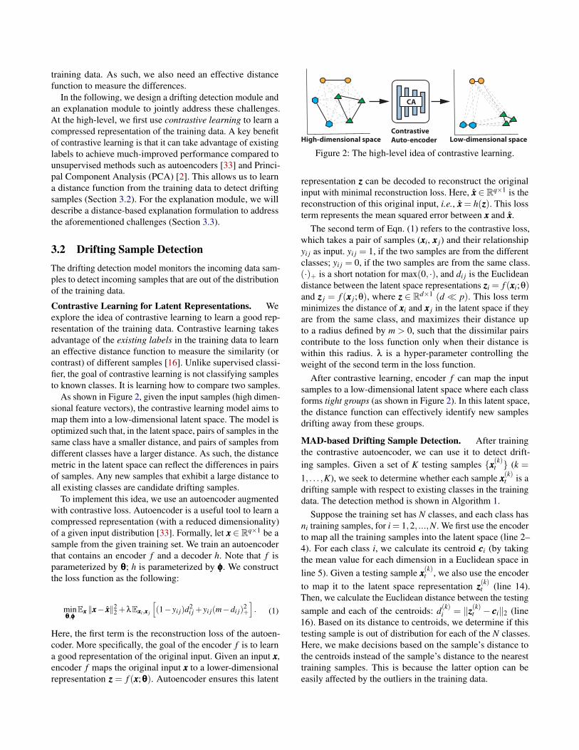
Contrastive Learning for Latent Representations. Weexplore the idea of contrastive learning to learn a good rep-resentation of the training data. Contrastive learning takesadvantage of the existing labels in the training data to learnan effective distance function to measure the similarity (orcontrast) of different samples [16]. Unlike supervised classi-fier, the goal of contrastive learning is not classifying samplesto known classes. It is learning how to compare two samples.

As shown in Figure 2, given the input samples (high dimen-sional feature vectors), the contrastive learning model aims tomap them into a low-dimensional latent space. The model isoptimized such that, in the latent space, pairs of samples in thesame class have a smaller distance, and pairs of samples fromdifferent classes have a larger distance. As such, the distancemetric in the latent space can reflect the differences in pairsof samples. Any new samples that exhibit a large distance toall existing classes are candidate drifting samples.

To implement this idea, we use an autoencoder augmentedwith contrastive loss. Autoencoder is a useful tool to learn acompressed representation (with a reduced dimensionality)of a given input distribution [33]. Formally, let xxx ∈ Rq×1 be asample from the given training set. We train an autoencoderthat contains an encoder f and a decoder h. Note that f isparameterized by θθθ; h is parameterized by φφφ. We constructthe loss function as the following:

minθθθ,φφφ

Exxx ‖xxx− xxx‖22 +λExxxi,xxx j

[(1− yi j)d2

i j + yi j(m−di j)2+

]. (1)

Here, the first term is the reconstruction loss of the autoen-coder. More specifically, the goal of the encoder f is to learna good representation of the original input. Given an input xxx,encoder f maps the original input xxx to a lower-dimensionalrepresentation zzz = f (xxx;θθθ). Autoencoder ensures this latent

High-dimensional space Low-dimensional space

CA

Contrastive

Auto-encoder

Figure 2: The high-level idea of contrastive learning.

representation zzz can be decoded to reconstruct the originalinput with minimal reconstruction loss. Here, xxx ∈ Rq×1 is thereconstruction of this original input, i.e., xxx = h(zzz). This lossterm represents the mean squared error between xxx and xxx.

The second term of Eqn. (1) refers to the contrastive loss,which takes a pair of samples (xxxi, xxx j) and their relationshipyi j as input. yi j = 1, if the two samples are from the differentclasses; yi j = 0, if the two samples are from the same class.(·)+ is a short notation for max(0, ·), and di j is the Euclideandistance between the latent space representations zzzi = f (xxxi;θ)and zzz j = f (xxx j;θ), where zzz ∈ Rd×1 (d� p). This loss termminimizes the distance of xxxi and xxx j in the latent space if theyare from the same class, and maximizes their distance upto a radius defined by m > 0, such that the dissimilar pairscontribute to the loss function only when their distance iswithin this radius. λ is a hyper-parameter controlling theweight of the second term in the loss function.

After contrastive learning, encoder f can map the inputsamples to a low-dimensional latent space where each classforms tight groups (as shown in Figure 2). In this latent space,the distance function can effectively identify new samplesdrifting away from these groups.

MAD-based Drifting Sample Detection. After trainingthe contrastive autoencoder, we can use it to detect drift-ing samples. Given a set of K testing samples {xxx(k)t } (k =

1, . . . ,K), we seek to determine whether each sample xxx(k)t is adrifting sample with respect to existing classes in the trainingdata. The detection method is shown in Algorithm 1.

Suppose the training set has N classes, and each class hasni training samples, for i = 1,2, ...,N. We first use the encoderto map all the training samples into the latent space (line 2–4). For each class i, we calculate its centroid ccci (by takingthe mean value for each dimension in a Euclidean space inline 5). Given a testing sample xxx(k)t , we also use the encoderto map it to the latent space representation zzz(k)t (line 14).Then, we calculate the Euclidean distance between the testingsample and each of the centroids: d(k)

i = ‖zzz(k)t − ccci‖2 (line16). Based on its distance to centroids, we determine if thistesting sample is out of distribution for each of the N classes.Here, we make decisions based on the sample’s distance tothe centroids instead of the sample’s distance to the nearesttraining samples. This is because the latter option can beeasily affected by the outliers in the training data.

Algorithm 1 Drift Detection with Contrastive Autoencoder.

Input: Training data xxx( j)i , i = 1, . . . ,N, j = 1, . . . ,ni, N is the number of

classes, ni is the number of training samples in class i; testing data xxx(k)t ,t refers to the testing set, k = 1, . . . , K, K is the total number of testingsamples; encoder f ; a constant b.

Output: Drifting score for each testing sample A(k), the closest class y(k)t ,centroid of each class ccci, MADi to each class.

1: for class i = 1 to N do2: for j = 1 to ni do3: zzz( j)

i = f (xxx( j)i ;θθθ) . The latent representation of xxx( j)

i .4: end for5: ccci =

1ni

∑nij=1 zzz( j)

i . The centroid of class i.6: for j = 1 to ni do7: d( j)

i = ||zzz( j)i − ccci||2 . The distance between sample and centroid.

8: end for9: di = median(d( j)

i ), j = 1, . . . ,ni

10: MADi = b∗median(|d( j)i − di|), j = 1, . . . ,ni

11: end for12:13: for k = 1 to K do14: zzz(k)t = f (xxx(k)t ;θθθ)15: for class i = 1 to N do16: d(k)

i = ||zzz(k)t − ccci||2

17: A(k)i =

|d(k)i −di |MADi

18: end for19: A(k) = min(A(k)

i ), i = 1, . . . ,N20: if A(k) > TMAD then . TMAD is set to 3.5 empirically [40].21: xxx(k)t is a potential drifting sample.22: else23: xxx(k)t is a non-drifting sample.24: end if25:26: y(k)t = argmin

id(k)

i , i = 1, . . . ,N . The closest class for xxx(k)t .

27: end for

To determine outliers based on d(k)i , the challenge is that

different classes might have different levels of tightness, andthus require different distance thresholds. Instead of manuallysetting the absolute distance threshold for each class, we usea method called Median Absolute Deviation (MAD) [40].The idea is to estimate the data distribution within eachclass i by calculating MADi (line 6–10), which is the me-dian of the absolute deviation from the median of distanced( j)

i ( j = 1, . . . ,ni). Here d( j)i depicts the latent distance be-

tween each sample in class i to its centroid, and ni is thenumber of samples in class i (line 7). Then based on MADi,we can determine if d(k)

i is large enough to make the testingsample xxx(k)t an outlier of class i (line 15–24). If the testingsample is an outlier for all of the N classes, then it is deter-mined as a drifting sample. Otherwise, we determine it isan in-distribution sample and its closest class is determinedby the closest centroid (line 26). The advantage of MAD isthat every class has its own distance threshold to determineoutliers based on its in-class distribution. For instance, if acluster is more spread out, the threshold would be larger.

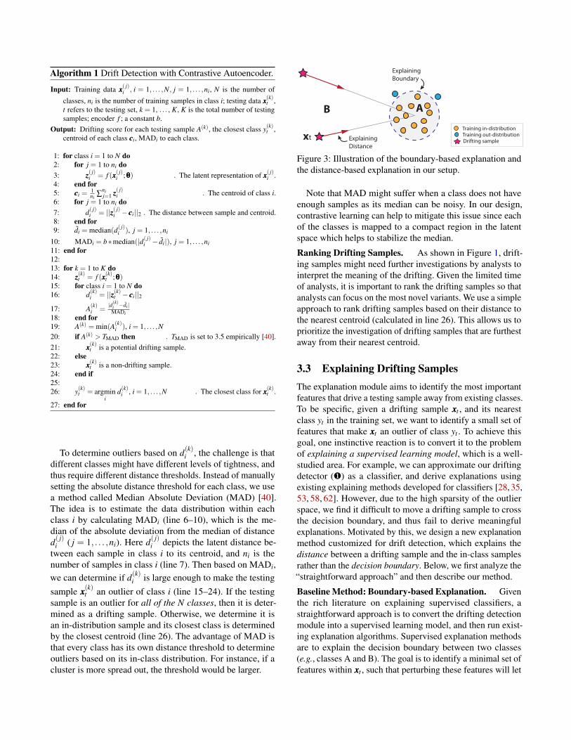
Explaining

Boundary

Explaining

DistanceDrifting sampleTraining out-distributionTraining in-distribution

AB

xt

Figure 3: Illustration of the boundary-based explanation andthe distance-based explanation in our setup.

Note that MAD might suffer when a class does not haveenough samples as its median can be noisy. In our design,contrastive learning can help to mitigate this issue since eachof the classes is mapped to a compact region in the latentspace which helps to stabilize the median.

Ranking Drifting Samples. As shown in Figure 1, drift-ing samples might need further investigations by analysts tointerpret the meaning of the drifting. Given the limited timeof analysts, it is important to rank the drifting samples so thatanalysts can focus on the most novel variants. We use a simpleapproach to rank drifting samples based on their distance tothe nearest centroid (calculated in line 26). This allows us toprioritize the investigation of drifting samples that are furthestaway from their nearest centroid.

3.3 Explaining Drifting SamplesThe explanation module aims to identify the most importantfeatures that drive a testing sample away from existing classes.To be specific, given a drifting sample xxxt , and its nearestclass yt in the training set, we want to identify a small set offeatures that make xxxt an outlier of class yt . To achieve thisgoal, one instinctive reaction is to convert it to the problemof explaining a supervised learning model, which is a well-studied area. For example, we can approximate our driftingdetector (¶) as a classifier, and derive explanations usingexisting explaining methods developed for classifiers [28, 35,53, 58, 62]. However, due to the high sparsity of the outlierspace, we find it difficult to move a drifting sample to crossthe decision boundary, and thus fail to derive meaningfulexplanations. Motivated by this, we design a new explanationmethod customized for drift detection, which explains thedistance between a drifting sample and the in-class samplesrather than the decision boundary. Below, we first analyze the“straightforward approach” and then describe our method.

Baseline Method: Boundary-based Explanation. Giventhe rich literature on explaining supervised classifiers, astraightforward approach is to convert the drifting detectionmodule into a supervised learning model, and then run exist-ing explanation algorithms. Supervised explanation methodsare to explain the decision boundary between two classes(e.g., classes A and B). The goal is to identify a minimal set offeatures within xxxt , such that perturbing these features will let

xxxt cross the decision boundary. As is shown in Figure 3, classA represents the in-distribution training samples from yt , andclass B represents the detected drifting sample in the testingset. The decision boundary is illustrated by the blue dashedline (the decision boundary is shown in the form of a norm ballsince it is based on distance threshold). Given a drifting sam-ple xxxt (denoted by a star in Figure 3), the explanation methodpulls the sample into the in-distribution class (i.e. the regionwith gray canvas) by perturbing a small set of important fea-tures.2 We implemented this idea using existing perturbation-based supervised explanation methods [13, 18, 21, 22] (imple-mentation details in Appendix A).

The evaluation result later in Section 5 shows that thisapproach is fundamentally limited. We believe the reasons aretwo-fold. First, given the limited number of drifting samples,it is difficult to derive an accurate approximation model for thedecision boundary. Second and more importantly, the outlierspace is much bigger than the in-distribution region. Giventhe drifting samples are far away from the decision boundary,it is difficult to find a small set of feature perturbations to takethe drifting sample to cross the decision boundary and enterthe in-distribution region. Without the ability to cross theboundary, the explanation methods do not have the necessarygradients (or feedback) to compute feature importance.

Our Method: Distance-based Explanation. Motivatedby this observation, we propose a new approach that identifiesimportant features by explaining the distance (i.e. the redarrow in Figure 3). Unlike supervised classifiers that makedecisions based on the decision boundary, the drift detectionmodel makes decisions based on the sample’s distance tocentroids. As such, we aim to find a set of original featuresthat help to move the drifting sample xxxt toward the nearestcentroid cccyt . With this design, we no longer need to force xxxtto cross the boundary, which is hard to achieve. Instead, weperturb the original features and observe the distance changesin the latent space.

To realize this idea, we need to first design a feature pertur-bation mechanism. Most existing perturbation methods aredesigned exclusively for images [18], the features of whichare numerical values. In our case, features in xxxt can be eithernumerical or categorical, and thus directly applying existingmethods will produce ill-defined feature values. To ensure theperturbations are meaningful for both numerical and categori-cal features, we propose to perturb xxxt by replacing its featurevalue with the value of the corresponding feature in a refer-ence training sample xxx(c)yt . This xxx(c)yt is the training sample thathas the shortest latent distance to the centroid cccyt . As such,our explanation goal is to identify a set of features, such thatsubstituting them with those in xxx(c)yt will impose the highestinfluence upon the distance between f (xxxt) and cccyt . Replacing

2Note that we do not perform feature perturbation in the latent space,because the latent features do not carry semantic meanings. Instead, we selectfeatures in the original input space.

the feature values with those of xxx(c)yt also helps to ensure theperturbed sample is moving towards the rough direction of thecentroid. As before, the perturbation is done in the originalfeature space where features have semantic meanings.

We use an mmm ∈Rq×1 to represent the important features, inwhich mmmi = 1 means (xxxt)i is replaced by the value of (xxx(c)yt )iand mmmi = 0 means we keep the value of (xxxt)i unchanged. Inother words, mmmi = 1 indicates the ith feature is selected asthe important one. Each element in this feature mask mmmi canbe sampled from a Bernoulli distribution with probabilitypi. As such, we could guarantee that mmmi equals to either 1and 0. Then, our goal is transformed into solving the pi fori = 1,2, ...,q. Technically, this can be achieved by minimizingthe following objective function with respect to p1:q.

Emmm∼Q(ppp)‖zzzt − cccyt‖2 +λ1R(mmm,bbb),

zzzt = f (xxxt � (1−mmm�bbb)+ xxx(c)yt � (mmm�bbb)),

R(mmm,bbb) = ‖mmm�bbb‖1 +‖mmm�bbb‖2, Q(ppp) =q

∏i=1

p(mmmi|pi).

(2)

Note that � denotes the element-wise multiplication; zzzt rep-resents the latent vector of the perturbed sample. Given theequation above, directly computing mmm is difficult due to itshigh dimensionality. To speed up the search, we introduce afilter bbb to pre-filter out features that are not worth considering.We set (bbb)i = 0, if (xxxt)i and (xxx(c)yt )i are the same. In otherwords, if a feature value of xxxt is already the same as that ofthe reference sample xxx(c)yt , then this feature is ruled out in theoptimization (since it has no impact on distance change). Inthis way, zzzt = f (xxxt� (1−mmm�bbb)+xxx(c)yt � (mmm�bbb)) representsthe latent vector of the perturbed sample.

In Eqn. (2), the first term in the loss function aims to mini-mize the latent-space distance between the perturbed samplezzzt and the centroid cccyt of the yt class. Each element in mmmis sampled from a Bernoulli distribution parameterized bypi. Here, we use Q(ppp) to represent their joint distribution.3

For the second term, λ is a hyper-parameter that controlsthe strength of the elastic-net regularization R(·), which re-stricts the number of non-zero elements in mmm. By minimizingR(mmm,bbb), the optimization procedure selects a minimum subsetof important features.

Note that Bernoulli distribution is discrete, which meansthe gradient of mmmi with respect to pi (i.e. ∂mmmi

∂pi) is not well de-

fined. We cannot solve the optimization problem in Eqn. 2 byusing a gradient-based optimization method. To tackle thischallenge, we apply the change-of-variable trick introducedin [45]. We enable the gradient computation by replacingthe Bernoulli distribution with its continuous approximation(i.e. concrete distribution) parameterized by pi. Then we cansolve the parameters p1:q through a gradient-based optimiza-tion method (we use Adam optimizer in this paper).

3We assume each feature is independently drawn from a distinct Bernoullidistribution.

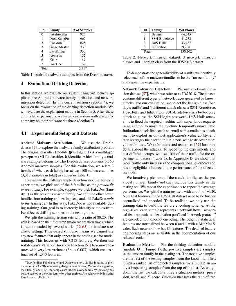
Id Family # of Samples0 FakeInstaller 9251 DroidKungFu 6672 Plankton 6253 GingerMaster 3394 BaseBridge 3305 Iconosys 1526 Kmin 1477 FakeDoc 132Total: 3,317

Table 1: Android malware samples from the Drebin dataset.

4 Evaluation: Drifting Detection

In this section, we evaluate our system using two security ap-plications: Android malware family attribution, and networkintrusion detection. In this current section (Section 4), wefocus on the evaluation of the drifting detection module. Wewill evaluate the explanation module in Section 5. After thesecontrolled experiments, we tested our system with a securitycompany on their malware database (Section 7).

4.1 Experimental Setup and Datasets

Android Malware Attribution. We use the Drebindataset [7] to explore the malware family attribution problem.The original classifier (module 0 in Figure 1) is a multilayerperceptron (MLP) classifier. It identifies which family a mal-ware sample belongs to. The Drebin dataset contains 5,560Android malware samples. For this evaluation, we select 8families 4 where each family has at least 100 malware samples(3,317 samples in total) as shown in Table 1.

To evaluate the drifting sample detection module, for eachexperiment, we pick one of the 8 families as the previouslyunseen family. For example, suppose we pick FakeDoc (fam-ily 7) as the previous unseen family. We split the other sevenfamilies into training and testing sets, and add FakeDoc onlyto the testing set. In this way, FakeDoc is not available dur-ing training. Our goal is to correctly identify samples fromFakeDoc as drifting samples in the testing time.

We split the training-testing sets with a ratio of 80:20. Thesplit is based on the timestamp (malware creation time), whichis recommended by several works [52, 65] to simulate a re-alistic setting. Time-based split also means we cannot useany new features that only appear in the testing set for modeltraining. This leaves us with 7,218 features. We then usescikit-learn’s VarianceThreshold function [51] to remove fea-tures with very low variance (i.e., <0.003), which creates afinal set of 1,340 features.

4Two families FakeInstaller and Opfake are very similar in terms of theirnature of attacks. There is strong disagreement among AV-engines regardingtheir family labels, i.e., the samples are labeled as one family by some enginesbut are labeled as the other family by other engines. As such, we only includedFakeInstaller (Table 1).

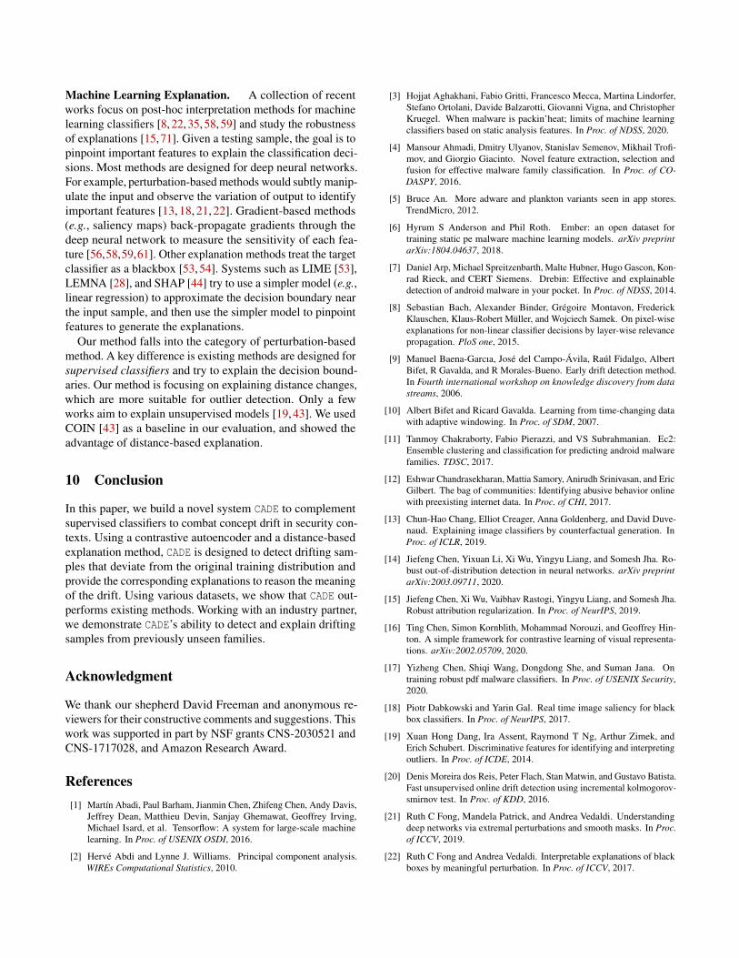
Id Family # of Flows0 Benign 66,2451 SSH-Bruteforce 11,7322 DoS-Hulk 43,4873 Infiltration 9,238Total: 130,702

Table 2: Network intrusion dataset: 3 network intrusionclasses and 1 benign class from the IDS2018 dataset.

To demonstrate the generalizability of results, we iterativelyselect each of the malware families to be the “unseen family”and repeat the experiments.

Network Intrusion Detection. We use a network intru-sion dataset [57], which we refer to as IDS2018. The datasetcontains different types of network traces generated by knownattacks. For our evaluation, we select the benign class (oneday’s traffic) and 3 different attack classes: SSH-Bruteforce,Dos-Hulk, and Infiltration. SSH-Bruteforce is a brute-forceattack to guess the SSH login password. DoS-Hulk attackaims to flood the targeted machine with superfluous requestsin an attempt to make the machine temporally unavailable.Infiltration attack first sends an email with a malicious attach-ment to exploit an on-host application’s vulnerability, andthen leverages the backdoor to run port-scan to discover morevulnerabilities. We refer interested readers to [57] for moredetails about the attacks. To speed up the experiments andtest different setups, we use 10% of their traffic for the ex-perimental dataset (Table 2). In Appendix D, we show thatmore traffic only increases the computational overhead andhas a negligible influence on the performance of the selectedmethods.

We iteratively pick one of the attack families as the pre-viously unseen family and only include this family in thetesting set. We repeat the experiments to report the averageperformance. We split the train-test sets with a ratio of 80:20.Note that features in the IDS2018 dataset need to be furthernormalized and encoded. To be realistic, we only use thetraining data to build the feature encoding scheme. At thehigh-level, each sample represents a network flow. Categori-cal features such as “destination port” and “network protocol”are encoded with one-hot encoding. The other 77 statisticalfeatures are normalized between 0 and 1 with a MinMaxS-caler. Each network flow has 83 features. The detailed featureengineering steps are available in the documentation of ourreleased code.

Evaluation Metric. For the drifting detection module(module ¶ in Figure 1), the positive samples are samplesin the unseen family in the testing set. The negative samplesare the rest of the testing samples from the known families.Given a ranked list of detected samples, we simulate an an-alyst inspecting samples from the top of the list. As we godown the list, we calculate three evaluation metrics: preci-sion, recall, and F1 score. Precision measures the ratio of true

0

0.2

0.4

0.6

0.8

1

0 100 200 300 400 500 600

Ra

te

Inspection Efforts (# of Samples)

PrecisionRecall

(a) CADE

0

0.2

0.4

0.6

0.8

1

0 100 200 300 400 500 600

Ra

te

Inspection Efforts (# of Samples)

PrecisionRecall

(b) Transcend

0

0.2

0.4

0.6

0.8

1

0 100 200 300 400 500 600

Ra

te

Inspection Efforts (# of Samples)

PrecisionRecall

(c) Vanilla AEFigure 4: Precision and recall vs. number of inspected samples (detected drifting samples are ranked by the respective method).

Method Drebin (Avg±Std) IDS2018 (Avg±Std)Precision Recall F1 Norm. Effort Precision Recall F1 Norm. Effort

Vanilla AE 0.63 ± 0.17 0.88 ± 0.13 0.72 ± 0.15 1.48 ± 0.31 0.61 ± 0.16 0.99 ± 0.00 0.74 ± 0.12 1.74 ± 0.40Transcend 0.76 ± 0.19 0.90 ± 0.14 0.80 ± 0.12 1.29 ± 0.45 0.64 ± 0.45 0.67 ± 0.47 0.65 ± 0.46 1.45 ± 0.57

CADE 0.96 ± 0.05 0.96 ± 0.04 0.96 ± 0.03 1.00 ± 0.09 0.98 ± 0.02 0.93 ± 0.09 0.96 ± 0.06 0.95 ± 0.07

Table 3: Drifting detection results for Drebin and IDS2018 datasets. We compare CADE with two baselines Transcend [38] andVanilla AE. For each evaluation metric, we report the mean value and the standard deviation across all the settings.

0

0.2

0.4

0.6

0.8

1

Drebin IDS2018

F1 S

core

Vanilla AE

Transcend

CADE

Figure 5: F1 scores of driftingdetection.

0.6

0.8

1

1.2

1.4

1.6

1.8

2

2.2

2.4

Drebin IDS2018

Norm

alized Invest. E

ffort

s

Vanilla AE

Transcend

CADE

Figure 6: Normalized investi-gation efforts.

unseen-family samples out of the inspected samples. Recallmeasures the ratio of unseen-family samples that are suc-cessfully discovered by the detection module out of all theunseen-family samples. F1 score is the harmonic mean of pre-cision and recall: F1 = 2× precision×recall

precision+recall . Finally, to quantifythe efforts of inspection, we define a metric called inspectingeffort, which is the total number of inspected samples, nor-malized by the number of true unseen family samples in thetesting set.

Baseline Methods. We include two main baselines. Thefirst baseline is a standard Vanilla autoencoder [33], whichis used to illustrate the benefit of contrastive learning. Weset the Vanilla autoencoder (AE) to have the same numberof layers and output dimensionality as CADE. We use it toperform dimension reduction to map the inputs into a latentspace where we use the same MAD method to detect andrank drifting samples. The difference between this baselineand CADE is that the baseline does not perform contrastivelearning. The hyperparameter setting is in Appendix B.

The second baseline is Transcend [38]. As described inSection 2, Transcend defines a “non-conformity measure” toquantify how well the incoming sample fits into the predictedclass, and calculate a credibility p-value to determine if theincoming sample is a drifting sample. We obtain the source

code of Transcend from the authors and follow the paper toadapt the implementation to support multi-class classifica-tion (the original code only supports binary classification).Specifically, we initialize the non-conformity measure with−p where p is the softmax output probability indicating thelikelihood that a testing sample belongs to a given family.Then we calculate the credibility p-value for a testing sample.If the p-value is near zero for all existing families, we considerit as a drifting sample. We rank drifting samples based on themaximum credibility p-value. Note that we did not use otherOOD detection methods [14, 41, 49] as our baseline mainlybecause they work in a different setup compared with CADEand Transcend. More specifically, these methods require anauxiliary OOD dataset in the training process and/or modi-fying the original classifier. These requirements are difficultto meet for malware classifiers in a production environment(detailed discussions are in Section 9).

4.2 Evaluation ResultsIn the following, we first compare the drifting detection per-formance of CADE with baselines and evaluate the impact ofcontrastive learning. Then, we perform case studies to investi-gate the potential reasons for detection errors.

Drifting Sample Detection Performance. We first useone experiment setting to explain our evaluation process.Take the Drebin dataset for example. Suppose we use familyIconosys as the previously unseen family in the testing set.After training the detection model (without any samples ofIconosys), we use it to detect and rank the drifting samples. Toevaluate the quality of the ranked list, we simulate an analystinspecting samples from the top of the list.

Figure 4a shows that, as we inspect more drifting samples(up to 150 samples), the precision maintains at a high level(over 0.97) while the recall gradually reaches 100%. Combin-

−50 −40 −30 −20 −10 0 10 20 30 40

−40

−20

0

20

40

(a) Original Space

−50 −40 −30 −20 −10 0 10 20 30 40

−40

−20

0

20

40

(b) Latent space (Vanilla AE)

−50 −40 −30 −20 −10 0 10 20 30 40

−40

−20

0

20

40FakeInstallerDroidKungFuPlanktonGingerMasterBaseBridgeIconosysKminFakeDoc

(c) Latent space (CADE)

Figure 7: T-SNE visualization for the original space, and latent spaces of Vanilla AE and CADE (unseen family: FakeDoc).

2

3

4

5

6

7

8

9

10

FakeInstaller

DroidKungFu

Plankton

GingerMaster

BaseBridge

Iconosys

KminFakeDoc

Dis

t. to n

eare

st centr

oid

Malware family used as unseen family

Non-driftDrift

(a) Original space

0

1

2

3

4

5

6

7

FakeInstaller

DroidKungFu

Plankton

GingerMaster

BaseBridge

Iconosys

KminFakeDoc

Dis

t. to n

eare

st centr

oid

Malware family used as unseen family

Non-driftDrift

(b) Latent space (CADE)

Figure 8: Boxplots of the distances between testing samples and their nearest centroids in both the original space and the latentspace for the Drebin dataset. Samples from previously unseen family are regarded as drifting samples.

ing precision and recall, the highest F1 score is 0.98. After150 samples, the precision will drop since there are no moreunseen family samples in the remaining set. This confirms thehigh-quality of the ranked list, meaning almost all the samplesfrom the unseen family are ranked at the top.

As a comparison, the ranked lists of Transcend and VanillaAE are not as satisfying. For Transcend (Figure 4b), the first150 samples return low precision and recall, indicating thetop-ranked samples are not from the unseen family. Afterinspecting 150 samples, we begin to see more samples fromthe unseen family. After inspecting 350 samples, Transcendhas covered most of the samples from the unseen family(i.e., with a recall near 1.0) but the precision is only 0.46.This means more than half of the inspected samples by theanalysts are irrelevant. The best F1 score is 0.63. As shown inFigure 4c, the performance of Vanilla AE is worse. The recallis only slightly above 0.8, even after inspecting 600 samples.

To generalize the observation, we iteratively take each fam-ily as the unseen family and compute the average statisticsacross different settings for F1 score (in Figure 5) and normal-ized inspecting efforts (in Figure 6). Table 3 further presentsthe corresponding precision and recall. For each experimentsetting, we report the highest F1 score for each model. ThisF1 score is achieved as the analysts go down the ranked listand stop the inspection when they start to get a lot of false

positives. The “inspecting effort” refers to the total number ofinspected samples to reach the reported F1 score, normalizedby the number of true drifting samples in the testing set.

Table 3 confirms that CADE can detect drifting samplesaccurately and outperforms both baselines. On Drebin, theaverage F1 score of CADE is 0.96, while the F1 scores for base-lines are 0.80 and 0.72. A similar conclusion can be drawnfor the IDS2018 dataset. In addition, the standard deviation ofCADE is much smaller than that of baselines, indicating a moreconsistent performance across different experiment settings.Finally, we show that CADE has lower normalized inspectingefforts, which confirms the high quality of the ranking.

Note that the Transcend baseline actually performs well incertain cases. For example, its F1 score is 99.69% (similar toour system) when DoS-Hulk is set as the unseen family in theIDS2018 dataset. However, the issue is Transcend’s perfor-mance is not stable in different settings, which is reflected inthe high standard deviations in Table 3.

Impact of Contrastive Learning. To understand thesource of the performance gain, we examine the impact ofcontrastive learning. First, we present a visualization in Fig-ure 7 which shows the t-SNE plot of the training samplesof the Drebin dataset and the testing samples from the cho-sen unseen family (FakeDoc). T-SNE [66] performs its own

non-linear dimensionality reduction to project data samplesinto a 2-d plot. To visualize our data samples, we map thesamples from the original space (1,340 dimensions) to a 2-dspace (Figure 7a). We also map the samples from the latentspace (7 dimensions) to the 2-d space as a comparison (Fig-ure 7b and Figure 7c). We can observe that samples in CADE’slatent space have formed tighter clusters, making it easier todistance existing samples from the unseen family.

To provide a statistical view of different experiment set-tings, we plot Figure 8. Like before, we iteratively take onefamily as the unseen family in Drebin. Then we measure thedistance of the testing samples to their nearest centroid inthe original feature space (Figure 8a) and the latent spaceproduced by CADE (Figure 8b). The results for the IDS2018dataset have the same conclusion, and thus are omitted forbrevity. We show that drifting samples and non-drifting sam-ples are more difficult to separate in the original space. Af-ter contrastive learning, the separation is more distinctive inthe latent space. The reason is that contrastive learning haslearned a suitable distance function that can stretch the sam-ples from different classes further apart, making it easier todetect unseen family.

Case Study: Limits of CADE. CADE performs well inmost of the settings. However, we find that in certain cases,CADE’s performance suffers. For example, when using Fake-Installer as the unseen family, our detection precision is only82% when the recall gets to 100%. We notice that many test-ing samples from GingerMaster and Plankton families weredetected as drifting samples. After a closer inspection, wefind that, when FakeInstaller is treated as the unseen family,in order to maintain the overall 80:20 training-testing ratio,we need to split the dataset at the time when there were notenough training samples from GingerMaster and Planktonyet. Therefore, many of the testing samples from GingerMas-ter and Plankton families look very different from the smallnumber of training samples in the two families (based onthe latent distance). External evidence also suggests that thetwo families had many variants [5, 70]. While these malwarevariants are not from a new family (false positives under ourdefinition), they could also have values for an investigation tounderstand malware mutation within the same family.

5 Evaluation: Explaining Drifting Samples

To evaluate the explanation module, we randomly select onefamily from each dataset (i.e. FakeDoc for Drebin and Infil-tration for IDS2018) as drifting samples. Results from othersettings have the same conclusion and thus are omitted forbrevity. Given this setting, we generate explanations for thedetected drifting samples and evaluate the explanation results,both quantitatively and qualitatively.

Method Drebin-FakeDoc IDS2018-InfiltrationAvg ± Std Avg ± Std

Original distance 5.363 ± 0.568 11.715 ± 2.321Random 5.422 ± 1.773 11.546 ± 3.169

Boundary-based 3.960 ± 2.963 6.184 ± 3.359COIN [43] 6.219 ± 3.962 8.921 ± 2.234

CADE 0.065 ± 0.035 2.349 ± 3.238

Table 4: Comparison of explanation fidelity based on the av-erage distance between the perturbed sample and the nearestcentroid. A shorter distance is better. “Original distance” isthe distance between the drift sample and nearest centroid.

5.1 Experimental Setup

Baseline Method. We consider three baseline methods:(1) a random baseline that randomly selects features as im-portant features; (2) the boundary-based explanation methoddescribed in Section 3, and (3) an unsupervised explanationmethod called COIN [43]. Due to space limit, we only brieflydescribe how COIN works. COIN builds a set of local Lin-earSVM classifiers to separate an individual outlier from itsin-distribution neighborhood samples. Since the LinearSVMclassifiers are self-explainable, they can pinpoint importantfeatures that contribute to the outlier classification. For afair comparison, we select the same number of top featuresfor baselines as our method. The implementation and hyper-parameters of these baselines can be found in Appendix B.Note that we did not select existing black-box explanationmethods (e.g., LIME [53] and SHAP [44]) as our comparisonbaselines. This is because white-box methods usually performbetter than black-box methods thanks to their access to theoriginal model [67].

Evaluation Metrics. Quantitatively, we directly evaluatethe impact of selected features on the distance changes. Givena testing sample xxxt and an explanation method, we obtainthe selected features mmmt , where (mmmt)i = 1, if the ith feature isselected as important, We quantify the fidelity of this expla-nation result by this metric: d′xxxt = ‖ f (xxxt � (1−mmmt)+ xxx(c)yt �mmmt)− cccyt‖2 where f , cccyt , and xxx(c)yt have the same definitionas the ones in Eqn. (2). d′xxxt represents the latent distance be-tween a perturbed sample of xxxt and its closet centroid cccyt .The perturbed sample is generated by replacing the values ofthe important features in xxxt with those of the training sampleclosest to the centroid (i.e. xxx(c)yt ). If the selected features aretruly important, then substituting them with the correspondingfeatures in the training sample from class yt will reduce thedistance between the perturbed sample and the centroid of cccyt .In this case, a lower distance d′xxxt is better.

In addition to this d′xxxt metric, we also use a traditionalmetric (Section 5.2) to examine the ratio of perturbed samplesthat can cross the decision boundary.

Drebin Case-A: Drifting Sample Family: FakeDoc; Closest Family: GingerMaster[api_call::android/telephony/SmsManager;->sendTextMessage] , [call::readSMS] , [permission::android.permission.DISABLE_KEYGUARD] ,

[permission::android.permission.RECEIVE_SMS] , [permission::android.permission.SEND_SMS] , [permission::android.permission.WRITE_SMS] ,

[real_permission::android.permission.SEND_SMS] , [permission::android.permission.READ_SMS] , [feature::android.hardware.telephony] ,

[permission::android.permission.READ_CONTACTS] , [real_permission::android.permission.READ_CONTACTS] ,[api_call::android/location/LocationManager;->isProviderEnabled], [api_call::android/accounts/AccountManager;->getAccounts],[intent::android.intent.category.HOME], [feature::android.hardware.location.network], [real_permission::android.permission.RESTART_PACKAGES] ,

[real_permission::android.permission.WRITE_SETTINGS] , [api_call::android/net/ConnectivityManager;->getAllNetworkInfo],[api_call::android/net/wifi/WifiManager;->setWifiEnabled], [api_call::org/apache/http/impl/client/DefaultHttpClient],[url::https://ws.tapjoyads.com/] , [url::https://ws.tapjoyads.com/set_publisher_user_id?] ,

[permission::android.permission.CHANGE_WIFI_STATE], [real_permission::android.permission.ACCESS_WIFI_STATE],[real_permission::android.permission.BLUETOOTH], [real_permission::android.permission.BLUETOOTH_ADMIN], [call::setWifiEnabled].

Table 5: Case study of explaining why a given sample a drifting sample. The highlighted features represent those that match thesemantic characteristics that differentiate the drifting sample with the closest family.

Method Drebin-FakeDoc IDS2018-InfiltrationRandom 0% 0%

Boundary-based 0% 0.41%COIN [43] 0% 0%

CADE 97.64% 1.41%

Table 6: Comparison of explanation fidelity based on theratio of perturbed samples that cross the decision boundary. Ahigher ratio means the perturbed features are more important.

5.2 Fidelity Evaluation Results

Feature Impact on Distance. Table 4 shows the meanand standard deviation for d′xxxt of all the drifting samples (i.e.,the distance between the perturbed samples to the nearestcentroid). We have four key observations. First, perturbingthe drifting samples based on the randomly selected featuresalmost does not influence the latent space distance (compar-ing Row 2 and 3). Second, the boundary-based explanationmethod could lower the distance by 26%–47% across twodatasets (comparing Row 2 and 4). This suggests this strat-egy has some effectiveness. However, the absolute distancevalues are still high. Third, COIN reduces the latent spacedistance on the IDS2018 dataset (comparing Row 2 and 5),but it somehow increases the average distance in the Drebindataset. Essentially, COIN is a specialized boundary-basedmethod that uses a set of LinearSVM classifiers to approx-imate the decision boundary. We find COIN does not workwell on the high-dimensional space, and it is difficult to dragthe drifting sample to cross the boundary (will be discussed inSection 5.3). Finally, our explanation module in CADE has thelowest mean and standard deviation for the distance metric.The distance has been reduced significantly from the origi-nal distance (i.e. 98.8% on Drebin and 79.9% on IDS2018,comparing Row 2 and 6). In particular, CADE significantly out-performs the boundary-based explanation method. Since ourmethod overcomes the sample sparsity and imbalance issues,it pinpoints more effective features that have a larger impacton the distance (which affects the drift detection decision).

Number of Selected Features. Overall, the number ofselected features is small, which makes it possible for manualinterpretation. As mentioned, we configure all the methods toselect the same number of important features (as CADE). Forthe Drebin dataset, on average the number of selected featuresis 44.7 with a standard deviation of 6.2. This is considered avery small portion (3%) out of 1000+ features. Similarly, theaverage number of selected features for the IDS2018 datasetis 16.2, which is about 20% of all the features.

5.3 Crossing the Decision Boundary

The above evaluation confirms the impact of the selectedfeatures on the distance metric, which is what CADE is de-signed to optimize. To provide another perspective, we furtherexamine the impact of the selected features on crossing theboundary. More specifically, we calculate the ratio of per-turbed samples that successfully cross the decision boundary.As shown in Table 6, we confirm that crossing the boundaryin the drifting detection context is difficult for most of thesettings. In particular, CADE can push 97.64% of the perturbedsamples to cross the detection boundary for the Drebin dataset,but only have 1.41% of the samples cross the boundary for theIDS2018 dataset. In comparison, the baseline methods canrarely successfully perturb the drifting samples in the originalfeature space to make them cross the boundary. By loosing upthis condition and focusing on distance changes, our methodis more effective in identifying important features.

5.4 Case Studies

To demonstrate our method indeed captures meaningful fea-tures, we present some case studies. In Table 5, we present acase study for the Drebin dataset. We take the setting whenFakeDoc is the unseen family and randomly pick a driftingsample to run the explanation module. Out of 1000+ features,our explanation module pinpointed 42 important features,among which 27 features have a value of “1” (meaning this

sample contains these features). As shown in Table 5, theclosest family is GingerMaster.

We manually examine these features to determine if thefeatures carry the correct semantic meanings. While it is dif-ficult to obtain the “ground-truth” explanations, we gatherexternal analysis reports about FakeDoc malware and Ginger-Master [68,70]. Based on these reports, a key difference fromGingerMaster is that FakeDoc malware usually subscribesto premium services via SMS and bill the victim users. Asshown in Table 5, many of the selected features are related topermissions and APIs calls for reading, writing, and sendingSMS. We highlight these features that match SMS relatedfunctionality. Other related features are highlighted too. Forexample, the permission of “RESTART_PACKAGES” allowsthe malware to end the background processes (e,g., that dis-plays incoming SMS) to avoid alerting the users. The per-mission of “DISABLE_KEYGUARD” allows the malware tosend premium SMS messages without unlocking the screen.“WRITE_SETTINGS” is also helpful to write system settingsfor sending SMS stealthily. “url::https://ws.tapjoyads.com/”is an advertisement library usually used by FakeDoc. Again,this small set of features is selected from over 1000 features.We conclude that these features are highly indicative of howthis sample is different from the nearest known family.

6 Evaluation: In-class Evolution

So far, our evaluation has been focused on one type of con-cept drift (Type A) where the drifting samples come froma previously unseen family. Next, we explore to adapt oursolution to address a different type of concept drift (Type B)where the drifting samples come from existing classes. Weconduct a brief experiment in a binary classification setting,following a similar setup with that of [38].

More specifically, we first use the Drebin dataset to traina binary SVM classifier to classify malware samples frombenign samples. The classifier is highly accurate on Drebinwith a training F1 score of 0.99. We want to test how wellthis classifier works on a different Android malware datasetMarvin [42]. Marvin is a slightly newer dataset (from 2010to 2014) compared with Drebin (from 2010 to 2012). We firstremove Marvin’s samples that are overlapped with those inDrebin, to make sure the Marvin samples are truly previouslyunseen. This left us 9,592 benign samples and 9,179 malwaresamples in Marvin.

For this experiment, we randomly split the Marvin datasetinto a validation set and a testing set (50:50). For both sets,we keep a balanced ratio of malware and benign samples.We apply the original classifier (trained on Drebin data) onthis Marvin testing set. We find that the testing accuracy is nolonger high (F1 score 0.70) due to potential in-class evaluationin the malware class and/or the benign class.

To address the in-class evolution, we apply CADE and Tran-scend on the Marvin validation set to identify a small number

# Selected Samples F1 of Retrained ClassifierCADE Transcend

0 0.70 0.70100 0.91 0.71150 0.92 0.76200 0.93 0.74250 0.94 0.71

Table 7: Performance of the retrained classifier on the Marvintesting set. We used CADE and Transcend to select the driftingsamples to be labeled for retraining.

of drifting samples (they could be either benign or malicious).We simulate to label them by using their “ground-truth” labelsand then add these labeled drifting samples back to the Drebintraining data to retrain the binary classifier. Finally, we testthe retrained classifier on the Marvin testing set.

As shown in Table 7, we find that CADE still significantlyoutperforms Transcend. For example, by adding only 150drifting samples (1.7% of Marvin validation set) for retraining,CADE boosts the binary classifier’s F1 score back to 0.92. ForTranscend, the same number of samples only gets the F1 scoreback to 0.74. In addition, we find that CADE is also faster: therunning time for CADE is 1.2 hours (compared to the 10 hoursof Transcend). This experiment confirms CADE can be adaptedto handle in-class evolution for a binary malware classifier.

7 Real-world Test on PE Malware

We have worked with the security company Blue HexagonInc. to test CADE on their proprietary sample set. More specif-ically, we run an initial test on Blue Hexagon’s Windowsmalware database. In this test, we got access to a set of sam-ples collected from August 29, 2019, to February 10, 2020.This set includes 20,613 unique Windows PE malware sam-ples from 395 families. We use this dataset to test CADE ina more diverse setup (i.e., the drifting samples come from alarger number of families).

PE Malware Dataset. For each sample, we have the rawbinary file and the metadata provided by Blue Hexagon, in-cluding the timestamp when the samples were first observed,and the family name (labeled by security analysts). We fol-low the feature engineering method of Ember [6], and useLIEF [63] to parse the binary files and extract the featurevectors. Each feature vector has 2,381 dimensions. These fea-tures include the frequency histogram of bytes and the entropyof different bytes, printable strings and special patterns, fea-tures about file size, header information, section information,imported libraries and functions, exported functions, and thesize and virtual addresses of data directories.

Family Attribution Experiments. The original classifieris a multi-class classifier to attribute malware families. Ourgoal is to use CADE to detect unseen families that should notbe attributed to existing families. We split the dataset based on

N Precision Recall F1 Norm. DetectedEffort Families

5 0.96 0.98 0.97 1.02 161/16510 0.96 0.94 0.95 0.98 153/16015 0.95 0.80 0.87 0.84 140/155

Table 8: Drifting detection results for the PE malware dataset.N is the number of known families in the training set. “De-tected Families” indicates the number of new families CADEdetected out of all the new families.

time. The training set contains the malware samples collectedfrom August 29 in 2019, to January 10 in 2020. The testingset contains samples collected in the following month, fromJanuary 10 to February 10, 2020. For training, we need tomake sure the malware families have enough samples to trainthe original classifier. So we focus on the top N families. Wetest three settings with N = 5, 10, and 15, respectively. Thismakes sure the training families contain at least 298 samplesper family in all the settings. Samples that are not in the topN families are excluded from the training set. Such a mini-mal number of samples is necessary for the original classifierto have reasonable accuracy. For example, the accuracy forN = 15 is 96.5%. The classifier can potentially support morefamilies if the dataset is larger. For the testing set, all the fam-ilies are kept. In addition, based on the suggestion from BlueHexagon’s analytics team, we add two families (Tinba andSmokeloader) to the testing set because they have observedthat these families have more success in evading existing ML-based malware detection engines. As shown in Table 8, thetesting set has 155 to 165 previously unseen families, i.e., thetarget of CADE.

Results and Case Studies. Table 8 shows that CADE stillperforms well under this diverse set of samples with morethan 155 previously unseen families. CADE achieves an F1score of 95% when the number of training families N = 10.The F1 score is still 0.87 when N = 15. Most of the previouslyunseen families are successfully identified. Indeed, a largernumber of families has made the problem more challenging.The reason is not necessarily because existing families andunseen families are difficult to separate. Instead, with moretraining families, we observe more testing samples withinthe existing families that drift even further away compared tothose in the unseen families. These in-family variants becomethe main contributor to false positives under our definition.The observation is similar to our case study in Section 4.2. Asa quick comparison, we also run Transcend on this N = 15setting. We find CADE still outperforms Transcend on the morediverse unseen families (Transcend’s F1 score is only 0.76).

We did a quick feature analysis using the explanation mod-ule on Tinba and Smokeloader which are proven to be chal-lenging examples for the underlying classifier. Tinba (tinybanker trojan) targets financial websites with man-in-the-browser attacks and network sniffing. Smokeloader is a trojanthat downloads other malware. It is an old malware family

but evolves rapidly. In particular, we find the new samples inTinba are closest to an existing family Wabot. CADE pinpoints45 features to offer explanations. For example, we find Tinbaenables the “LARGE_ADDRESS_AWARE” option, whichtells the linker that the program can handle addresses largerthan 2 gigabytes. This option is enabled by default on 64-bitcompilers. This provides some explanation on why Tinba hasthe success in evading existing malware detection engines,given that the vast majority of PE malware files are 32-bitbased. Based on features about “sections,” we notice that theTinba sample uses “UPX” as the packer. Based on selectedfeatures of imported libraries and functions, we find Tinbaimports “crypt32.dll” for encrypting strings. Tinba samplesare different from Wabot samples on these features.

8 Discussion

Computational Complexity. CADE’s computational over-head is smaller than existing methods. The complexity ofthe detection module contains two parts: contrastive learningand drifting detection. The complexity of contrastive learn-ing is O(IB2|θ|), where I, B, and |θ| represent the number oftraining iterations, batch size, and model parameters of the au-toencoder. The complexity of drifting detection (Algorithm 1)is O(Nni+NK), where N, ni, and K are the number of classes,the maximum number of training samples in each class, andthe number of testing samples, respectively. The overall com-plexity of CADE detection module is O(IB2|θ|+Nni +NK).Our training overhead is acceptable since it is only quadraticto the batch size B. Our detection runtime overhead is sig-nificantly lower than that of Transcend (which is O(NniK)).Empirically, we have recorded the average runtime for thedetection experiments (Section 4), and confirms that CADE isfaster than Transcend. For example, on the larger IDS2018dataset, the average run time for CADE and Transcend are1,422.7s and 4,289.3s. Regarding the explanation module,CADE is comparable with boundary-based explanation meth-ods and COIN. For example, for the IDS2018 dataset, theaverage runtime of CADE, COIN, and boundary-based explana-tion for explaining one drifting sample are 3.2s, 8.2s, and 3.7srespectively. The boundary-based explanation also requiresan additional 76.5s on average to build the approximationmodel for the explanation.

Explanation vs. Adversarial Attacks. We notice that theexplanation module in CADE shares some similarities withthe adversarial example generation process, e.g., both involveperturbing the given input for a specific objective. However,we think they are different for two reasons. First, they havedifferent outputs. Adversarial attack (with the goal of evasion)directly outputs the perturbation needed to cross the decisionboundary; Our explanation method (with the goal of under-standing the drift) outputs the important features that affectthe distance. Second, they have different constraints on the

perturbations. Our explanation method only tries to minimizethe number of perturbed features, while the adversarial attackconstrains the magnitude of the perturbation too. More impor-tantly, adversarial samples need to be valid for the respectiveapplications (i.e., valid malware samples that can be executedand maintain the malicious behavior, valid network flows thatcan carry out the original attack). To these ends, generatingadversarial samples can be more difficult than deriving ex-planations in our context. That said, the adversarial attack isout of the scope of this paper. We leave adversarial attacksagainst CADE to future work (i.e., creating non-perceptibleperturbation to convert a drifting sample to an in-distributionsample).

Limitations and Future Work. Our work has a few limi-tations. First, CADE ranks all the drifting samples in a singlelist. However, in practice, the drifting samples may containsubstructures (e.g., multiple new malware families). A practi-cal strategy could be further grouping drifting samples intoclusters. In this way, security analysts only need to inspectand interpret a few representative samples per cluster to fur-ther save time. Second, certain hyper-parameters of CADE aredetermined empirically (e.g., the MAD threshold). We haveincluded an Appendix C to test the sensitivity of CADE tohyper-parameters. Future work can look into more systematicstrategies to configure the hyper-parameters. Third, CADE isdesigned based on the assumption that the training set doesnot have mislabeled samples (or poisoning samples). We de-fer to future work to robustify our system against low-qualityor malicious labels. Fourth, our experiments are primarily fo-cused on detecting new families. In Section 6, we only brieflyexperimented with concept drift within existing families (in-class evolution). We defer a more in-depth analysis to futurework.

Finally, our evaluation in Section 7 is limited to N = 15training classes (and 155 previously unseen testing classes).We limited to N = 15 to make sure each training class hasenough samples to train an accurate original classifier. Totest a larger N, we tried to apply CADE to several other mal-ware datasets but did not find a suitable one that could meetour need. For example, the Ember-2018 dataset [6] providesmalware samples from a large number of families. However,the family labels are not well curated. For instance, a pop-ular malware family name in Ember-2018 is called “high”(8,417 samples) which turns out to be incorrectly parsed fromVirusTotal reports: the original entry name in the reports is“Malicious (High Confidence),” which is not a real malwarefamily name. We have observed other similar parsing errorsand inconsistencies in the labels. The Ember-2017 dataset [6]and the UCSB packed malware dataset [3] do not provide mal-ware family information. The dataset from Microsoft MalwareClassification Challenge [55] only has 9 malware families,which is smaller than our Blue Hexagon dataset. Given ourunsuccessful efforts, we defer the examination of a largernumber of training classes to future work.

9 Related work

Machine Learning used in Security. Machine learninghas been used to solve many security problems such as mal-ware detection [6,7,17,42], malware family attribution [4,11],and network intrusion detection [24, 34, 48, 60]. More re-cently, researchers look into using deep learning methods toperform binary analysis [27, 69], software vulnerability iden-tification [72], and severity prediction [30]. Most of thesemachine learning models need to address the concept driftproblem when deployed in practice.

Out of Distribution (OOD) Detection. Recently, themachine learning community has made progress in out-of-distribution detection [14, 32, 41, 46, 49]. These works arerelevant, but have different assumptions and goals comparedto ours. At the high-level, most of these methods try to cal-ibrate the “probability” produced by the original classifierto detect OOD samples. The researchers indeed recognizedthat the probability could be untrustworthy when it comes topreviously unseen distributions [14, 32]. To avoid assigninga high probability to an OOD sample, the proposed methodsusually need to introduce an auxiliary OOD dataset to thetraining data. These methods are difficult to realize in securityapplications for two reasons. First, auxiliary OOD dataset (i.e.,previously unseen attacks) is extremely difficult to obtain inthe first place. Second, these solutions require re-designingthe original classifier (e.g., a functional malware detector),which is inconvenient to do in the production environment.Instead, our method does not rely on auxiliary OOD datasetand is decoupled from the original classifier.

Classification Trustworthiness. A related line of workaims to assess the trustworthiness of the classification re-sults [11, 37, 50]. A common goal is to identify untrustedpredictions, e.g., predictions on adversarial attacks. Most ofthese methods are based on the idea of “nearest neighbors”.The intuition is, an untrusted prediction is more likely tohave a different label from its nearest neighbors. For example,DkNN [50] derives a trust score by comparing a testing sam-ple with its neighboring training samples at each layer of aDeep Neural Network (DNN). Another recent work [37] com-pute the trust score based on the neighboring “high-density-sets”. However, such neighbor-based methods still rely ona good distance function. As acknowledged in [37], theirmethod may suffer in a high dimensional space. Overall,these methods are focused on different problems from ours.Their goal is to identify misclassifications within existingclasses (not drifting samples from new classes). Another sys-tem EC2 [11] uses a threshold of prediction probability tofilter out untrustworthy predictions. Related to this direction,active learning methods also use prediction probability toselect low-confidence samples to be labeled for model retrain-ing [47, 73]. As discussed before (see [32]), the predictionprobability itself can be misleading under concept drift.

Machine Learning Explanation. A collection of recentworks focus on post-hoc interpretation methods for machinelearning classifiers [8, 22, 35, 58, 59] and study the robustnessof explanations [15,71]. Given a testing sample, the goal is topinpoint important features to explain the classification deci-sions. Most methods are designed for deep neural networks.For example, perturbation-based methods would subtly manip-ulate the input and observe the variation of output to identifyimportant features [13, 18, 21, 22]. Gradient-based methods(e.g., saliency maps) back-propagate gradients through thedeep neural network to measure the sensitivity of each fea-ture [56,58,59,61]. Other explanation methods treat the targetclassifier as a blackbox [53, 54]. Systems such as LIME [53],LEMNA [28], and SHAP [44] try to use a simpler model (e.g.,linear regression) to approximate the decision boundary nearthe input sample, and then use the simpler model to pinpointfeatures to generate the explanations.

Our method falls into the category of perturbation-basedmethod. A key difference is existing methods are designed forsupervised classifiers and try to explain the decision bound-aries. Our method is focusing on explaining distance changes,which are more suitable for outlier detection. Only a fewworks aim to explain unsupervised models [19, 43]. We usedCOIN [43] as a baseline in our evaluation, and showed theadvantage of distance-based explanation.

10 Conclusion

In this paper, we build a novel system CADE to complementsupervised classifiers to combat concept drift in security con-texts. Using a contrastive autoencoder and a distance-basedexplanation method, CADE is designed to detect drifting sam-ples that deviate from the original training distribution andprovide the corresponding explanations to reason the meaningof the drift. Using various datasets, we show that CADE out-performs existing methods. Working with an industry partner,we demonstrate CADE’s ability to detect and explain driftingsamples from previously unseen families.

Acknowledgment

We thank our shepherd David Freeman and anonymous re-viewers for their constructive comments and suggestions. Thiswork was supported in part by NSF grants CNS-2030521 andCNS-1717028, and Amazon Research Award.

References[1] Martín Abadi, Paul Barham, Jianmin Chen, Zhifeng Chen, Andy Davis,

Jeffrey Dean, Matthieu Devin, Sanjay Ghemawat, Geoffrey Irving,Michael Isard, et al. Tensorflow: A system for large-scale machinelearning. In Proc. of USENIX OSDI, 2016.

[2] Hervé Abdi and Lynne J. Williams. Principal component analysis.WIREs Computational Statistics, 2010.

[3] Hojjat Aghakhani, Fabio Gritti, Francesco Mecca, Martina Lindorfer,Stefano Ortolani, Davide Balzarotti, Giovanni Vigna, and ChristopherKruegel. When malware is packin’heat; limits of machine learningclassifiers based on static analysis features. In Proc. of NDSS, 2020.

[4] Mansour Ahmadi, Dmitry Ulyanov, Stanislav Semenov, Mikhail Trofi-mov, and Giorgio Giacinto. Novel feature extraction, selection andfusion for effective malware family classification. In Proc. of CO-DASPY, 2016.

[5] Bruce An. More adware and plankton variants seen in app stores.TrendMicro, 2012.

[6] Hyrum S Anderson and Phil Roth. Ember: an open dataset fortraining static pe malware machine learning models. arXiv preprintarXiv:1804.04637, 2018.

[7] Daniel Arp, Michael Spreitzenbarth, Malte Hubner, Hugo Gascon, Kon-rad Rieck, and CERT Siemens. Drebin: Effective and explainabledetection of android malware in your pocket. In Proc. of NDSS, 2014.

[8] Sebastian Bach, Alexander Binder, Grégoire Montavon, FrederickKlauschen, Klaus-Robert Müller, and Wojciech Samek. On pixel-wiseexplanations for non-linear classifier decisions by layer-wise relevancepropagation. PloS one, 2015.

[9] Manuel Baena-Garcıa, José del Campo-Ávila, Raúl Fidalgo, AlbertBifet, R Gavalda, and R Morales-Bueno. Early drift detection method.In Fourth international workshop on knowledge discovery from datastreams, 2006.

[10] Albert Bifet and Ricard Gavalda. Learning from time-changing datawith adaptive windowing. In Proc. of SDM, 2007.

[11] Tanmoy Chakraborty, Fabio Pierazzi, and VS Subrahmanian. Ec2:Ensemble clustering and classification for predicting android malwarefamilies. TDSC, 2017.

[12] Eshwar Chandrasekharan, Mattia Samory, Anirudh Srinivasan, and EricGilbert. The bag of communities: Identifying abusive behavior onlinewith preexisting internet data. In Proc. of CHI, 2017.

[13] Chun-Hao Chang, Elliot Creager, Anna Goldenberg, and David Duve-naud. Explaining image classifiers by counterfactual generation. InProc. of ICLR, 2019.

[14] Jiefeng Chen, Yixuan Li, Xi Wu, Yingyu Liang, and Somesh Jha. Ro-bust out-of-distribution detection in neural networks. arXiv preprintarXiv:2003.09711, 2020.

[15] Jiefeng Chen, Xi Wu, Vaibhav Rastogi, Yingyu Liang, and Somesh Jha.Robust attribution regularization. In Proc. of NeurIPS, 2019.

[16] Ting Chen, Simon Kornblith, Mohammad Norouzi, and Geoffrey Hin-ton. A simple framework for contrastive learning of visual representa-tions. arXiv:2002.05709, 2020.

[17] Yizheng Chen, Shiqi Wang, Dongdong She, and Suman Jana. Ontraining robust pdf malware classifiers. In Proc. of USENIX Security,2020.

[18] Piotr Dabkowski and Yarin Gal. Real time image saliency for blackbox classifiers. In Proc. of NeurIPS, 2017.

[19] Xuan Hong Dang, Ira Assent, Raymond T Ng, Arthur Zimek, andErich Schubert. Discriminative features for identifying and interpretingoutliers. In Proc. of ICDE, 2014.

[20] Denis Moreira dos Reis, Peter Flach, Stan Matwin, and Gustavo Batista.Fast unsupervised online drift detection using incremental kolmogorov-smirnov test. In Proc. of KDD, 2016.

[21] Ruth C Fong, Mandela Patrick, and Andrea Vedaldi. Understandingdeep networks via extremal perturbations and smooth masks. In Proc.of ICCV, 2019.

[22] Ruth C Fong and Andrea Vedaldi. Interpretable explanations of blackboxes by meaningful perturbation. In Proc. of ICCV, 2017.

[23] João Gama, Indre Žliobaite, Albert Bifet, Mykola Pechenizkiy, andAbdelhamid Bouchachia. A survey on concept drift adaptation. ACMcomputing surveys (CSUR), 2014.

[24] Pedro Garcia-Teodoro, Jesus Diaz-Verdejo, Gabriel Maciá-Fernández,and Enrique Vázquez. Anomaly-based network intrusion detection:Techniques, systems and challenges. Computers & Security, 2009.

[25] Ian J Goodfellow, Jonathon Shlens, and Christian Szegedy. Explainingand harnessing adversarial examples. Proc. of ICLR, 2015.

[26] Antonio Gulli and Sujit Pal. Deep learning with Keras. 2017.

[27] Wenbo Guo, Dongliang Mu, Xinyu Xing, Min Du, and Dawn Song.Deepvsa: Facilitating value-set analysis with deep learning for post-mortem program analysis. In Proc. of USENIX Security, 2019.

[28] Wenbo Guo, Dongliang Mu, Jun Xu, Purui Su, Gang Wang, and XinyuXing. Lemna: Explaining deep learning based security applications. InProc. of CCS, 2018.

[29] Raia Hadsell, Sumit Chopra, and Yann LeCun. Dimensionality reduc-tion by learning an invariant mapping. In Proc. of CVPR, 2006.

[30] Zhuobing Han, Xiaohong Li, Zhenchang Xing, Hongtao Liu, and Zhiy-ong Feng. Learning to predict severity of software vulnerability usingonly vulnerability description. In Proc. of ICSME, 2017.

[31] Maayan Harel, Shie Mannor, Ran El-Yaniv, and Koby Crammer. Con-cept drift detection through resampling. In Proc. of ICML, 2014.

[32] Dan Hendrycks and Kevin Gimpel. A baseline for detecting misclassi-fied and out-of-distribution examples in neural networks. In Proc. ofICLR, 2017.

[33] Geoffrey E Hinton and Ruslan R Salakhutdinov. Reducing the dimen-sionality of data with neural networks. Science, 2006.

[34] Elike Hodo, Xavier Bellekens, Andrew Hamilton, Christos Tachtatzis,and Robert Atkinson. Shallow and deep networks intrusion detectionsystem: A taxonomy and survey. arXiv preprint arXiv:1701.02145,2017.

[35] Sara Hooker, Dumitru Erhan, Pieter-Jan Kindermans, and Been Kim.A benchmark for interpretability methods in deep neural networks. InProc. of NeurIPS, 2019.

[36] Steve TK Jan, Qingying Hao, Tianrui Hu, Jiameng Pu, Sonal Oswal,Gang Wang, and Bimal Viswanath. Throwing darts in the dark? detect-ing bots with limited data using neural data augmentation. In Proc. ofS&P, 2020.

[37] Heinrich Jiang, Been Kim, Melody Guan, and Maya Gupta. To trust ornot to trust a classifier. In Proc. of NeurIPS, 2018.

[38] Roberto Jordaney, Kumar Sharad, Santanu K Dash, Zhi Wang, DavidePapini, Ilia Nouretdinov, and Lorenzo Cavallaro. Transcend: Detectingconcept drift in malware classification models. In Proc. of USENIXSecurity, 2017.

[39] Alex Kantchelian, Sadia Afroz, Ling Huang, Aylin Caliskan Islam,Brad Miller, Michael Carl Tschantz, Rachel Greenstadt, Anthony D.Joseph, and J. D. Tygar. Approaches to adversarial drift. In Proc. ofAISec, 2013.

[40] Christophe Leys, Christophe Ley, Olivier Klein, Philippe Bernard, andLaurent Licata. Detecting outliers: Do not use standard deviationaround the mean, use absolute deviation around the median. Journal ofExperimental Social Psychology, 2013.

[41] Shiyu Liang, Yixuan Li, and Rayadurgam Srikant. Enhancing thereliability of out-of-distribution image detection in neural networks.Proc. of ICLR, 2018.

[42] Martina Lindorfer, Matthias Neugschwandtner, and Christian Platzer.Marvin: Efficient and comprehensive mobile app classification throughstatic and dynamic analysis. In Prof. of COMPSAC, 2015.

[43] Ninghao Liu, Donghwa Shin, and Xia Hu. Contextual outlier interpre-tation. In Proc. of IJCAI, 2018.

[44] Scott M. Lundberg and Su-In Lee. A unified approach to interpretingmodel predictions. In Proc. of NeurIPS, 2017.

[45] Chris J Maddison, Andriy Mnih, and Yee Whye Teh. The concretedistribution: A continuous relaxation of discrete random variables. InProc. of ICLR, 2017.

[46] Marc Masana, Idoia Ruiz, Joan Serrat, Joost van de Weijer, and Anto-nio M Lopez. Metric learning for novelty and anomaly detection. InProc. of BMVC, 2018.

[47] Brad Miller, Alex Kantchelian, Sadia Afroz, Rekha Bachwani, EdwinDauber, Ling Huang, Michael Carl Tschantz, Anthony D. Joseph, andJ.D. Tygar. Adversarial active learning. In Proc. of AISec, 2014.

[48] Yisroel Mirsky, Tomer Doitshman, Yuval Elovici, and Asaf Shabtai.Kitsune: an ensemble of autoencoders for online network intrusiondetection. In Proc. of NDSS, 2018.

[49] Aristotelis-Angelos Papadopoulos, Mohammad Reza Rajati, NazimShaikh, and Jiamian Wang. Outlier exposure with confidence controlfor out-of-distribution detection. arXiv preprint arXiv:1906.03509,2019.

[50] Nicolas Papernot and Patrick McDaniel. Deep k-nearest neighbors: To-wards confident, interpretable and robust deep learning. arXiv preprintarXiv:1803.04765, 2018.

[51] F. Pedregosa, G. Varoquaux, A. Gramfort, V. Michel, B. Thirion,O. Grisel, M. Blondel, P. Prettenhofer, R. Weiss, V. Dubourg, J. Vander-plas, A. Passos, D. Cournapeau, M. Brucher, M. Perrot, and E. Duch-esnay. Scikit-learn: Machine learning in Python. Journal of MachineLearning Research, 2011.

[52] Feargus Pendlebury, Fabio Pierazzi, Roberto Jordaney, Johannes Kinder,and Lorenzo Cavallaro. TESSERACT: Eliminating experimental biasin malware classification across space and time. In Proc. of USENIXSecurity, 2019.

[53] Marco Tulio Ribeiro, Sameer Singh, and Carlos Guestrin. "why shouldi trust you?" explaining the predictions of any classifier. In Proc. ofKDD, 2016.

[54] Marco Tulio Ribeiro, Sameer Singh, and Carlos Guestrin. Anchors:High-precision model-agnostic explanations. In Proc. of AAAI, 2018.

[55] Royi Ronen, Marian Radu, Corina Feuerstein, Elad Yom-Tov, and Man-sour Ahmadi. Microsoft malware classification challenge. arXivpreprint arXiv:1802.10135, 2018.

[56] Ramprasaath R Selvaraju, Michael Cogswell, Abhishek Das, Ramakr-ishna Vedantam, Devi Parikh, and Dhruv Batra. Grad-cam: Visualexplanations from deep networks via gradient-based localization. InProc. of ICCV, 2017.

[57] Iman Sharafaldin, Arash Habibi Lashkari, and Ali A Ghorbani. To-ward generating a new intrusion detection dataset and intrusion trafficcharacterization. In Prof. of ICISSP, 2018.

[58] Avanti Shrikumar, Peyton Greenside, and Anshul Kundaje. Learningimportant features through propagating activation differences. In Proc.of ICML, 2017.

[59] Karen Simonyan, Andrea Vedaldi, and Andrew Zisserman. Deep insideconvolutional networks: Visualising image classification models andsaliency maps. Workshop at ICLR, 2014.

[60] Robin Sommer and Vern Paxson. Outside the closed world: On usingmachine learning for network intrusion detection. In Proc. of S&P,2010.

[61] Jost Tobias Springenberg, Alexey Dosovitskiy, Thomas Brox, and Mar-tin Riedmiller. Striving for simplicity: The all convolutional net. InProc. of ICLR, 2015.

[62] Mukund Sundararajan, Ankur Taly, and Qiqi Yan. Axiomatic attributionfor deep networks. In Proc. of ICML, 2017.

[63] Romain Thomas. Lief - library to instrument executable formats.https://lief.quarkslab.com/, April 2017.

[64] Robert Tibshirani and Guenther Walther. Cluster validation by pre-diction strength. Journal of Computational and Graphical Statistics,2005.

[65] Daniele Ucci, Leonardo Aniello, and Roberto Baldoni. Survey ofmachine learning techniques for malware analysis. Computers &Security, 2019.

[66] Laurens van der Maaten and Geoffrey Hinton. Visualizing data usingt-SNE. Journal of Machine Learning Research, 2008.

[67] Alexander Warnecke, Daniel Arp, Christian Wressnegger, and KonradRieck. Don’t paint it black: White-box explanations for deep learningin computer security. In Proc. of Euro S&P, 2020.

[68] Fengguo Wei, Yuping Li, Sankardas Roy, Xinming Ou, and Wu Zhou.Deep ground truth analysis of current android malware. In Proc. ofDIMVA, 2017.

[69] Xiaojun Xu, Chang Liu, Qian Feng, Heng Yin, Le Song, and DawnSong. Neural network-based graph embedding for cross-platformbinary code similarity detection. In Proc. of CCS, 2017.

[70] Rowland Yu. Ginmaster: a case study in android malware. In Virusbulletin conference, 2013.

[71] Xinyang Zhang, Ningfei Wang, Shouling Ji, Hua Shen, and Ting Wang.Interpretable deep learning under fire. In Proc. of USENIX Security,2020.

[72] Yaqin Zhou, Shangqing Liu, Jingkai Siow, Xiaoning Du, and Yang Liu.Devign: Effective vulnerability identification by learning comprehen-sive program semantics via graph neural networks. In Proc. of NeurIPS,2019.

[73] Jingbo Zhu, Huizhen Wang, Eduard Hovy, and Matthew Ma.Confidence-based stopping criteria for active learning for data annota-tion. ACM Trans. Speech Lang. Process., 2010.

[74] Arthur Zimek, Erich Schubert, and Hans-Peter Kriegel. A survey onunsupervised outlier detection in high-dimensional numerical data.Statistical Analysis and Data Mining, 2012.

Appendix A: Boundary-based Explanation

To perform the boundary-based explanation, we first need toapproximate the detection boundary of the drift detection mod-ule with a parametric function. We need to run approximationbecause the true boundary of the drift detector is threshold-based, which is not parametric. Specifically, we used an MLPclassifier to perform the approximation in the latent space.Due to the limited number of drifting samples, to approximatethe decision boundary, we first synthesized more drifting sam-ples by adding Gaussian noise to the latent representations ofthe detected drifting samples. Then, we trained an MLP g(zzz)to classify the latent representations of the in-distribution sam-ples from the drifting samples. After obtaining the approxima-tion model, we combined it with the contrastive autoencoderf to construct a supervised approximation of the detectionmodule (i.e. g( f (xxx))). We conducted the approximation inthe latent space rather than the input space for two reasons.First, training an MLP in a low dimensional space is moreefficient than in a high dimensional space. Second, directlyutilizing the original contrastive autoencoder enables a higherfidelity of the supervised approximation than approximatingthe autoencoder with another network. Using the supervisedapproximation, we then applied the perturbation-based expla-nation method [22] to explain each drifting sample. Similar to

CADE, this method also outputs a mask indicating the featureimportance. We ranked the mmmi and pinpointed the featureswith high mmmi as the important ones.

Appendix B: CADE Implementation Details

CADE. We implemented CADE based on the Keras [26]package with Tensorflow [1] as the backend. The hyper-parameters of CADE and the baselines are configured as thefollowing. As for CADE, we set the encoder as an MLP withthe architecture of 1340-512-128-32-7 for the Drebin dataset(the first dimension could vary when using different familiesas the unseen family) and 83-64-32-16-3 for the IDS2018dataset. The activation function for each hidden layer is theReLU function. We applied the Adam optimizer with thelearning rate of 0.0001 and epochs of 250 to train both net-works. The batch size for Drebin and IDS2018 are 32 and256, respectively. As for the hyper-parameters introduced bythe contrastive loss in Eqn. (1), we set λ = 0.1 and m = 10.We applied the widely used empirical value for the MADthreshold and coefficient: TMAD = 3.5 and b = 1.4826. Forthe hyper-parameters introduced by the explanation loss inEqn. (2), we set λ1 = 1e− 3 and used the Adam optimizerwith the learning rate of 0.01 to solve the optimization func-tion. The training epoch is set as 250.

Drift Detection Baselines. The vanilla autoencoder base-line was implemented as a variant of our system without usingcontrastive learning. We also implemented a multi-class ver-sion of Transcend based on the source code provided by theauthors. The hyper-parameters of the vanilla AE baselineare almost the same with CADE except for the MAD thresh-old TMAD = 0. We tried TMAD = 3.5 for this method, whichresulted in zero precision and recall. The reason is that the dis-tance in vanilla AE’s latent space is not optimized to comparedifferent samples and thus MAD lost its effectiveness.

For Transcend, we used an MLP with the architecture of1340-100-30-7 for the Drebin dataset and 83-30-3 for theIDS2018 dataset to train a multi-class classifier. Then weused the negative output probability−p as the non-conformitymeasure of Transcend. We set the threshold of the credibilityp-value as 1.0. That is, a testing sample is marked as a driftingsample if its p-value is lower than 1.0.

Explanation Baselines. We implemented the boundary-based explanation method and the random selection as de-scribed in the main text. For COIN, we used the source codereleased by the authors as the implementation.5 The net-work architectures of the approximation function g in theboundary-based explanation are 7-15-2 and 3-15-2 for Drebinand IDS2018, respectively. The optimizer, batch size, andnumber of epochs are the same as those used in our sys-

5https://github.com/ninghaohello/Contextual-Outlier-Interpreter

Parameter Drebin (Avg±Std) IDS2018 (Avg±Std)F1 Norm. Effort F1 Norm. Effort

m = 5 0.95 ± 0.05 0.97 ± 0.05 0.72 ± 0.39 0.72 ± 0.39m = 10 0.96 ± 0.03 1.00 ± 0.09 0.96 ± 0.06 0.95 ± 0.07m = 15 0.91 ± 0.06 1.00 ± 0.14 0.77 ± 0.33 0.76 ± 0.34m = 20 0.93 ± 0.03 1.06 ± 0.13 0.98 ± 0.02 1.02 ± 0.02

λ = 1 0.95 ± 0.03 1.05 ± 0.11 0.94 ± 0.09 1.00 ± 0.00λ = 0.1 0.96 ± 0.03 1.00 ± 0.09 0.96 ± 0.06 0.95 ± 0.07

λ = 0.01 0.94 ± 0.03 1.05 ± 0.09 0.67 ± 0.47 0.71 ± 0.42λ = 0.001 0.89 ± 0.10 1.19 ± 0.33 0.95 ± 0.05 0.93 ± 0.08

TMAD = 2.0 0.96 ± 0.03 1.00 ± 0.09 0.94 ± 0.09 0.99 ± 0.02TMAD = 2.5 0.96 ± 0.03 1.00 ± 0.09 0.95 ± 0.07 0.97 ± 0.04TMAD = 3.0 0.96 ± 0.03 1.00 ± 0.09 0.95 ± 0.07 0.96 ± 0.05TMAD = 3.5 0.96 ± 0.03 1.00 ± 0.09 0.96 ± 0.06 0.95 ± 0.07

Table 9: Sensitivity test of three hyper-parameters on detectingdrifting samples. For each evaluation metric, we report themean value and the standard deviation across all the settings.

λ1 Drebin-FakeDoc IDS2018-Infiltrationdistance (Avg ± Std) Ratio distance (Avg ± Std) Ratio

0.1 0.119 ± 0.058 91.34% 2.669 ± 3.343 1.99%0.01 0.085 ± 0.039 96.85% 2.403 ± 3.266 1.36%

0.001 0.065 ± 0.035 97.64% 2.349 ± 3.238 1.41%0.0001 0.064 ± 0.027 99.21% 2.322 ± 3.240 1.69%

Table 10: Sensitivity test on the hyper-parameter λ1 of ex-plaining a drifting sample. “Ratio” means the percentage ofperturbed samples that cross the decision boundary.

tem. The hyper-parameters of solving the explanation masks(i.e. optimizer and epoch) are also the same as our system.Finally, we used the default choices of the hyper-parametersfrom the authors’ code of COIN.

The original implementation of COIN provided by the au-thors can be very slow when the dataset has a large numberof samples and outliers. For each detected outlier, COIN runsKMeans clustering on its 10% of nearest neighbors to get itscontexts. To determine the best number of clusters (K), COINiterates K from 1 to a pre-defined threshold and adopts themeasure of prediction strength [64] to assess the choice ofK. Prediction strength can be computationally expensive asit requires pair-wise comparison on the labels predicted byKMeans. To make it feasible, on the large IDS2018 dataset,we only choose 1% of nearest neighbors and fix the number ofclusters as a value between 1 and 4 for each outlier. Also, theLinearSVM classifier does not converge on about 6% of out-liers even we set max iterations as 200,000. We report the bestaverage result on the converged cases obtained from COIN.For the Drebin dataset, we keep all the hyper-parameters thesame as the original code.

Appendix C: Hyper-parameter Sensitivity

In Section 3.2, the loss function of contrastive autoencoderhas two hyper-parameters: λ and m. Here, we evaluate thesensitivity of CADE’s performance to these hyper-parameters.Our experiment methodology is to fix one parameter andswap the other one. We fix λ as 0.1 and set m as 5, 10, 15,

Sampling Rate 10% 15% 20% 25% 30%F1 score 0.96 0.98 0.98 0.98 0.97

Table 11: Sampling rate of IDS2018 dataset vs. F1 score ofCADE.

20. As shown in Table 9, CADE achieves a high F1 score onthe Drebin dataset when m = 5 and m = 10, but has someminor degradation on m = 15 and m = 20. The detectionperformance on the IDS2018 dataset is good when m is set toa higher number e.g., m = 20. Recall that m is the thresholdto control the upper-bound distance that will be considered. Adissimilar pair can contribute to the loss function only whentheir distance is within the radius of m. As such, m can be setto be higher if the dataset is more dispersed and noisy.

To test the effect of λ, we fix m = 10 as before, and set λ as1, 0.1, 0.01, and 0.001. λ controls the weight of the contrastiveloss. We can observe from Table 9 that if λ is too small, ithurts CADE’s performance. The results confirm the importanceof the contrastive loss.

In Algorithm 1, we set the threshold of MAD TMAD as 3.5,which is an empirical value [40]. We also tested other com-monly used MAD thresholds of 2, 2.5, 3. A smaller MADthreshold will detect more samples as potential drifting sam-ples, but it may not affect the ranking procedure. As shown inTable 9, the average results of the detected drifting sampleskeep the same as TMAD = 3.5 on Drebin and minor fluctu-ations on the IDS2018 dataset, indicating TMAD has subtleeffects on detecting drifting samples.

To assess the sensitivity of the hyper-parameter λ1 in theloss function (Eqn.( 2)) of distance-based explanation, weset λ1 as 0.1, 0.01, 0.001, and 0.0001. As shown in Table 10,we notice that smaller λ1 can have a slightly smaller averagedistance to the nearest centroid on both Drebin and IDS2018datasets. Also, a smaller λ1 can increase the ratio of perturbedsamples that cross the decision boundary from 91.34% to99.21% on Drebin-FakeDoc. While for IDS-Infiltration, theratio could vary on different values of λ1. But overall, bothevaluation metrics do not have significant differences amongdifferent values of λ1.

Appendix D: IDS2018 Additional Results

In our experiment, we only sampled 10% of the network traf-fic from the IDS2018 dataset. Traffic sampling is a commonapproach in intrusion detection, which allows us to compre-hensively test different experimental setups. We also find thatincluding more traffic only increases the computational over-head and has a negligible influence upon the performance. Asshown in Table 11, as the sampling rate increases, CADE’s F1scores remain consistently high.