David B. Davidson Dept E&E Engineering University of Stellencosch Stellenbosch 7600 South Africa (+27) 21 808 4458 (+27) 21 808 4981 (Fax) davidson@firgo sun oc LO (e-moil)

, John L. Volakis Rad tab EECSDept University of Michigan Ann Arbor MI 48109 2122 (734) 647-1 797 (734) 647 2106 (Fax) volakis0umich edu (email)

Forward by JLV

I am very pleased to announcc that David Davidson will hereafier co-edit the EM Programmer’s Notebook. David obtained his BEng and MEng degrees from lhe University of Pretoria (1983, 1986), and the PhD degree from the University of Stellenbosch (South Akica) in 1991. He is presently a Profcssor in lhe Depart- ment of Elcctrical and Electronic Engineering at the University of Stellenbosch. David has worked extensively on computational techniques for electromagnetics, including FDTD, Moment Method and finite-element techniques. We arc indeed very pleased that hc joined the editorial staff of the Magazine, and look forward to his participation and input. David will hc primarily responsible for contributions from Asia and Europe. Please feel free to direct any such EM Programmer’s Notebook contributions to David.

In this issne of the EM Programmer’s Notebook, Jim Roedder of Boeing-St. Louis rcvisits high-frequency computations on the basis of ray-tracing methods. As is well known, ray-tracing algorithms can utilize shadowing-data information, available from the hardware or softwarc z-buffer of thc workstation, to speed up ray-tracing algorithms by more than a fiictor of 10. Moreover, ray- tracing algorithms can work directly from IGES surface formats, and thus avoid discretization or facetization of the geometry itself. This increases geometry fidelity, but more accurate shadowing is necessary in low-scattering regions. In this issue’s paper, trimmed lGES surfaces are considered to improve the accuracy of high-fre- quency codes based on ray tracing.

CADDSCAT Version 2.3: A High-Frequency Physical Optics Code Modified for Trimmed IGES B-Spline Surfaces James M. Roedder The Boeing Company Mail Code SO642263 PO B O X 516 St. Louis, MO 63166

Keywords: Physical optics, ray tracing, B spline, electromagnetic scattering, radar cross section

1. Background

Graphics Exchange Spccification (IGES) file format. The snhset of IGES [Z] entitics supported are the 114 and 128 curved-parametric- surface entities.

B-spline surfaces are defined parametrically over a paramet- ric rectangle. A B-spline surface becomes “trimmed“ for geome-

wing passes through a fuselage. The B-spline surface is trimmed by reducing the domain of the surface irom the entire parametric rectangle to a smaller portion of that domain, delineated by “trim cnmes.” (Sce references [4] and [ 5 ] for more an this topic.) Most PO codes require that B-spline surfaces be free of trims. The requirement to remove trims from a geometric model by rebuilding surfaces can increase the design time.

hysical-Optics (PO) cadcs using curved-surface representations

While freeing the radar-signature engincer from performing tedi- ous “facetization” of highly complex target models, curved-surface codes slill impose a burden on the person configuring the design That burden is the requirement to provide a geometric model that is appropriate to thc PO formulation, which accommodates only a subset of thc normally available design entities. Since 1988, CAD models have been imported into CADDSCAT via the lnitial

IEEEAntennaS ondPropogat ion Magazine. Vo l . 41. No. 3. J u n e 1999

P of targets have been in existence for morc than 12 years [I]. tries where surface-surfxe intersections occur, such as when a

69

Within the electromagnetics community, methods to perform first-bounce PO computations using workstation graphics softwarel hardware for acceleration are sometimes given the misnomer ''2

-buffer" [3]. r-buffer-based codes, such as GRECO, provide a par- tial solution far accommodating trimmed IGES models. However, z-buffer is not suitable for low-observable (LO) targets where higher-fidelity PO current modeling is required. As a result, the Boeing CADDSCAT code [ l ] has been modified to allow trimmed IGES B-spline surfaces. (B-spline surfaces will be referred to sim- ply as "B surfaces" throughout the rest of this paper.)

2. Alternative approaches to accommodate trims

The z-buffer method relies on standard graphics packages (such as OpenGL or Starbase) to solve the trim-line problem. Such packages draw to the graphics screen only surface components that should he visible. Thus, z-buffer accommodates both cast shad- owing (blockage) and trim-line effects directly. Because the method utilizes graphics hardware to perform PO computations, it can be more than an order of magnitude faster than conventional first-bounce PO computations, performed as integrations in sur- face-parametric space. However, the method is not adequate for LO targets. Figure 1 compares the CADDSCAT and GRECO (a z- buffer-based code) scattering results at I O GHz for a cubic chine body-of-translation, representative of a chined fighter side-wall. The angle sweep passes through the principal plane of this target. The GRECO results were calculated by Dr. Juan Rius in 1997. As can clearly be seen, z-buffer provides insufficient accuracy for electrically large targets at shallow grazing angles (elevation less 30 degrees in the figure). The problem is that for electrically large targets, there is an inadequate number of screen pixels to sample the PO current at shallow incidence, where the phase of the current is rapidly changing.

Another approach is to convert the trimmed geometry model into a finely triangulated mesh. However, this can result in the well-known "facet noise" in the radar cross section (RCS) [l]. In hopes of overcoming the facet-noise problem, other aerospace organizations have used as many as one million facets for fighter- size aircraft. However, faceting the target model sets the effective frequency bandwidth of the model; the curved-surface representa- tion is the best wide-bandwidth model.

3. CADDSCATapproach

CADDSCAT does not take the facetization approach. Instead, trimmed IGES surfaces are input to CADDSCAT exactly as speci- fied, by the person configuring the design, in the IGES file. Those original surfaces, along with the required trims, are then utilized in the PO and ray-tracing algorithms.

The CADDSCAT code performs numerical integrations to assess curved-surface PO. This has been described in [I]. For most types of surfaces, the "ribbon" technique (Figure 2) is used to reduce the integration in one parametric direction to analytic form, leaving the other parametric direction to be integrated numerically.

3.1 Trim curves and trimmed surfaces

This paper assumes a basic knowledge of parametric-spline curves and parametric surfaces. If the reader is not familiar with these, two classic texts, Geometric Modelling by Mortenson [4] and A Practical Guide to Splines by deBoor [6] , give excellent

detailed discussions. The CADDSCAT algorithm for handling trimmed surfaces is not limited to B-splines, and has functioned properly for other low-order-polynomial spline types, such as the IGES 112 entity (i.e., parametric-spline curve). Since even experi- enced readers may be unfamiliar with B-splines, a short summary is included here for completeness.

A rational B-spline curve is expressed parametrically by

~

70 IEEEAntennas OndPropogat ion Mogazine, V o l . 41. No. 3. J u n e 1999

Figure 1. An RCS analysis of a chined body-of-translation at 10 GHz. The angle sweep is in the principal plane.

. B M e F0m6 "Rlbtmn- Tcchniqu, Technique

Sampbs Spaced iB Apart in U and w

mtegtmn 1s &I* in Either U or w

u - U -- Figure 2. Curved-surface integration methods.

where G(f)is a spline of degree M, with N segments and N+1

breakpoints at T ( 0 ) ,..., T ( N ) ; K i s equal to N + M - I ; and the

b ( t ) are the “B-spline basis functions.” The basis functions are

determined recursively from a “knot sequence” T ( - M ) ,..., T(O),

.._, T ( N ) , ..., T ( N + M ) . The “B” in B-spline is simply an abbre-

nation for “basis.” The P(i) are the curve “control points.” The

w(i) are the control-point “weights:” these determine how close

the curve stays to the control points. The larger the weight for an index i, the closer the curve approaches control point i. If all the weights are unity, the curve is not rational, and the denominator can be ignored.

A rational B-spline surface is also expressed parametrically by

where S(u,w) is a surface of degree MI in U and degree M 2 in

w. It has NI patches and NI+Ibreak points, U ( O ) , U ( I ) ,..., U ( N 1 ) in U , and N2 patches and N 2 t 1 break points

W(O),W(I) ,...,E‘( N 2 ) in w. IC1 is equal to N l + M I - I ; K 2 is,

equal to N 2 + M 2 - 1. The b, (U) are the U basis functions, derived

from the U knot sequence. The P( i , j ) are the w basis functions.

derived from the W knot sequence. The W(i, j ) are the surface: control-point “weights.”

Trim curves in an IGES file describe the U and w values of hounding curves as a function of a parameter, 1. That is, the U ancl w trim-curve values are both functions of the independent parame- ter, f. Trim c w e s can he of two types: “outer” and “inner.” An IGES trim entity (entity 144) specifies zero or one outer trirri boundaries, and zero or more inner trim boundaries. An arbitraq number of trim holes can he specified by one trim entity. Holes in surfaces are represented hy “inner” trim boundaries. The outei: extents of B surfaces are limited by “outer” trim boundaries. Even if a B surface is not trimmed, IGES files sometimes provide an outer trim houndav that encompasses the entire B surface para. metric rectangle. Presumably, this is so that a single “branch” of software can he used to process both trimmed and untrimmed EL surfaces. By convention, the portion of a surface that is “kept” (inside the trimming region) is to the left of a trim curve, when the trim curve is traversed in the direction of increasing f.

In the present paper, a “patch“ is defined to be a portion of a B surface spanning the parametric interval between adjacent con- trol-curve knots. If the patch is a parametric hi-cubic surface, it can be described by 48 floating-point coefficients. Reference [SI describes a procedure that replaces the patch and its arbitrarily complex trim-line arrangement with a set of simpler “regions.” CADDSCAT uses a similar procedure, discussed in this paper.

3.2 Definition of a “region”

The CADDSCAT approach partitions the parametric rectangle of each patch into a set of parametric “regions,” which can be described by

~

IEEEAnTennas and Propagation Magazine, Vol . 41, No. 3, June 1999 71

1. Minimum and maximum iv boundaiy constants:

2. A left-hand B-spline bounding-trim-curve segmcnt or minimum U boundary constant; and

3. A right-hand B-spline bounding-trim-curve segment or maxi- mum U boundary constant.

“Left-hand“ here refers to the left-hand border of the region in parametric space. A left-hand limit ciirvc defines the minimum U

limit for the region at various w parametric values. A “right-hand trim curve is defined similarly. The rcgion information is auto- matically assembled during a prc-processing step, and retained for subsequent surface rendering, PO analysis, and ray tracing.

The trim curves that impact each trimmed patch must be identified. This is done by finding various characteristics of the trim curves as these relate to the B surface as a whole, and then, in a subsequent step, mapping the trim curves (and their effects) to individual patches. Individual patches fall into three categories: a.) not trimmed, h.) partially trimmed, and c.) completely trimmed away.

A trim-curve identifier, relevant trim-curve parameter (usu- ally denoted by I), and a U and w parametric pair (in B-surface parametric space) are computed for each of the following trim- c w e quantities:

Local extrema: Local extrema of all trim curves-i.e., maximdminima of trim-curve U and w values-are calculated in B- surface parametric space. This is perfonned analytically by finding the real roots of the first derivative (with respect to I) of each seg- ment of each trim curve. There might also he extrema at locations in the knot sequence where either the knot value or the control point is duplicated (see [6]).

Intersections with knots: The intersections of him curves with all B-surface knots, both u-knots and w-knots, are found. This step is also executed entirely analytically, since all trim-curve B- spline c w e s are polynomial, i.e., not rational. In addition, trim curves are low-order polynomials. These knot intersections are the “entry” points of trim curves onto individual patches.

Curve endpoints: All trim-curve endpoints, distinct from all the above-mentioned points, are calculated. The joins of individual B-spline curves of a composite curve must he considered end- points.

3.3 Classifying patches

As noted above, individual patches are classified as not trimmed, partially trimmed, or comp1el.ely trimmed. To determine if a patch is partially trimmed, all o f the above (u,w) pairs are tested against the U-knot and w-knot intervals that define the border of the patch. If any of the (u,w) coordmates are inside the knot interval, the patch is partially trimmed and parametric “regions” must he assigned to that patch (discussed in the next section).

If there are no (u.w) pairs inside the patch knot interval, the patch is either not trimmed at all, or completely trimmed away. The foilowing evedodd crossings mle is used to make the deter- mination:

The number of trim boundary intersections with the U and w knot Sines between the patch border and the edge

Y --

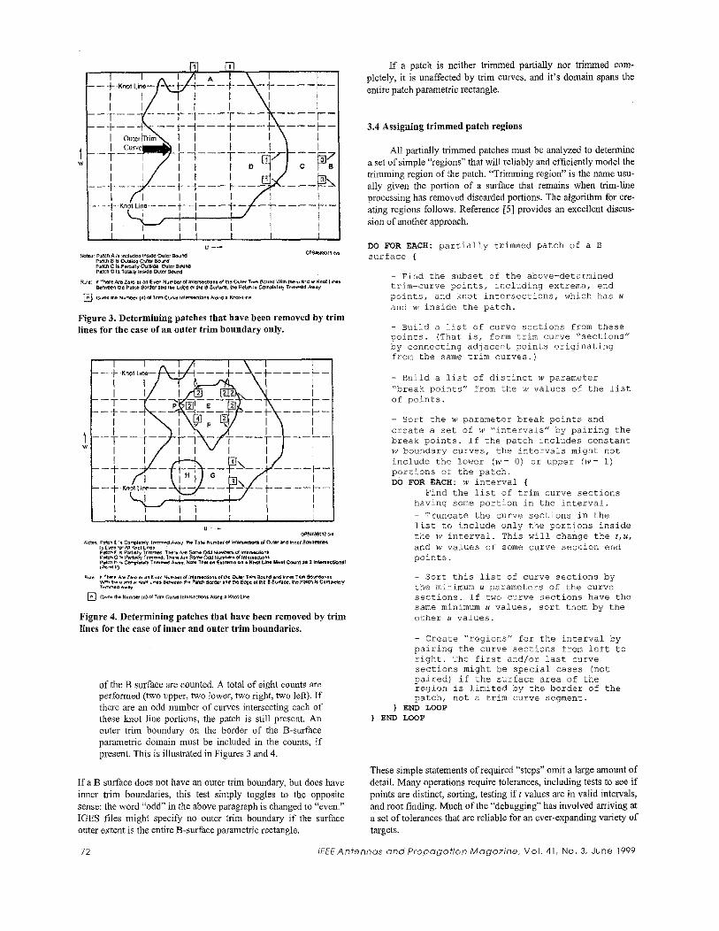
Figure 3. Determining patches that have been removed by trim lines for the case of an outer trim boundary only.

Figure 4. Determining patches that have been removed by trim lines for the case of inner and outer trim boundaries.

of the B surface are counted. A total of eight counts are performed (two upper, two lower, two right, two left). If there are an odd number of cumes intersecting each of these h o t line portions, the patch is still present. An outer trim boundary on the border of the B-surface parametric domain must he included in the counts, if present. This is illustrated in Figures 3 and 4.

If a B surface does not have an outer trim boundary, but does have inner trim boundaries, this test simply toggles to the opposite sense: the word "odd" in the above paragraph is changed to "even." IGES files might specify no outer trim boundary if the surface outer extent is the entire B-surface parametric rectangle.

If a patch is neither trimmed partially nor trimmed com- pletely, it is unaffected by trim curves, and it's domain spans the entire patch parametric rectangle.

3.4 Assigning trimmed patch regions

All partially trimmed patches must be analyzed to determine a set of simple "regions" that will reliably and efficiently model the trimming region of the patch. "Trimming region" is the name usu- ally given the portion of a surface that remains when trim-line processing has removed discarded portions. The algorithm for cre- ating regions follows. Reference [SI provides an excellent discus- sion of another approach.

DO FOR EACH: partially trimmed patch of a B surface I

- Find the subset of the above-determined trim-curve points, including extrema, end points, and knot intersections, which has U and w inside the patch.

- Bu~ld a list of curve sections from these points. (That is, form trim curve "sections" by connecting adlacent points originating from the same trim curves.)

- Build a list of distinct w parameter "break points" from the w values of the list of points.

72 iEEEAntennos ondPropoQoiion Mogorine. V o l . 41. N O . 3. June 1999

- Sort the w parameter break points and create a set of w "intervals" by pairing the break points. If the patch includes Constant w boundary curves, the intervals might not include the lower ( w = 0 ) or upper ( w = 1) portions of the patch. DO FOR EACH: w interval I

~ Find the list of trim curve sections having some portion in the interval. ~ Truncate the curve sections in the list to include only the portions inside the w interval. This will change the f , u , and w va lues of some curve section end points.

- Sort this list of curve sections by the minimum U parameters of the curve sections. If two curve sections have the same minimum U values, sort them by the other U values.

- Create "regions" far the interval by pairing the curve sections from left to right. The first and/or last curve sections might be special cases (not paired) if the sur face area of the region is limited by the border of the patch, not a trim curve segment.

) END LOOP END LOOP

These simple statements of required "steps" omit a large amount of detail. Many operations require tolerances, including tests to see if points are distinct, sorting, testing iff values are in valid internals, and root finding. Much of the "debugging" has involved arriving at a set of tolerances that are reliable for an ever-expanding variety of targets.

Figure Sa. MrPafches trim processing for the following three targets with trim processing disabled (trim lines are shown in red): cyl-trim-hole. iges, cyl-trim-slice. iges, and in red). cyl-trimwedge.iges.

Figure 5b. MrPaiches trim processing for the three targets of Figure 5a with trim processing enabled (trim lines are shown

Figure Se. Mrl'aiches trim processing for the three targets of Figure 5a with ray-trace-trimmed targets (single-bounce rays are not shown).

Figure 7. The ray-trace footprint (shadow) of a trimmed patch. Figure 9a. The geometry for the trimmed pillow target. The figure shows two IGES files separalely (upper portion) and together (lower portion). The trim lines are shown as thick lines.

/€€€Antennas ond Propagotion Mogazine, Vo l . 41, No 3, J u n e 1999 73

The trimmed upper component of Figure I is a single “patch,” as defined above, with a number of trim holes. A large number of parallel ray traces have been launched at this target. The impact points of rays that reach the patch at the bottom of the fig- ure are displayed as dots. The trimmed patch of this figure is probably not typical of geometries for which RCS analysis is desired. However, the geometry demonstrates the robustness of the above algorithm in processing complicated trim lines. The one (1) trimmed patch has more than one hundred (100) regions.

At this time, not all possible trim-cuke arrangements are properly processed in CADDSCAT, As the algorithms continue to he “field tested,” they are improved. Very complex targets have been processed without error. If the appearance of any B surface is incorrect in MrPaiches, the trims From only that surface should he removed. The author is most familiar with geometries originating from Unigraphics. Problems in these geometries have heen:

a. Trim lines that double hack over themselves (to a very slight degree, of course)

b. Trim lines that do the loop; such that there are slight differences between beginning and ending points of trim-curve loops.

It is tempting to declare problems such as (a) and (b) to be ”hugs” in the Unigraphics implementation. It only makes sense to provide trim curves in closed loops of cunres that do not cross. A simple approach to repair the (b) problems has been included in the CADDSCA T B-surface pre-processing.

Figure 6a. MrPatclies trim processing of an axleibracket target with trim processing disabled.

Figure 6b. MrPatches trim processing of an axleibracket target with trim processing enabled.

3.5 Viewing trimmed surfaces

CADDSCAT provides users wiih a visual verification capa- bility to ensure Llnl trim proccssing is being performed correctly. This is accomplished through the Mn%tches graphical code [7], which is used to draw and ray trace the trimmed geometry. The logic in MrPaiches for trim-surface rendering is similar to that used by the CADDSCAT PO-integration algorithms. It uses the same description of the patch regions as used in the PO numerical algorithms (see Note 1. ) MrPatches ray tracing operates exactly as in CmDSCAT, since MYPutches and CADDSCAT share the same geometry package, GEOMPACK [Ref 81. Thus, if surface-shape inspections and ray tracing of the model in MvPafches seem rea- sonable, the RCS processing will he correct. Figures 5 , 6, and 7 depict examples of MrPutches trim-line processing and ray tracing of several simple targets (See Note 2).

3.6 First-bounce physical-optics computations

To calculate trimmed-surface PO, the CADDSCAT two- dimensional (two-dimensional) Gaussian-integration algorithm (i.e., “Brute Force Algorithm” on the left side ofFigure 2) has been converted from FORTRAN to C++. This is required since geome- try information, e.g., him-curve data and region descriptions, are stored in C data structures.

C t t algorithms are sometimes “slow,” at least when com- pared with equivalent FORTRAN or C algorithms. Using standard C++ programming techniques, the CADDSCAT C++ PO algo- rithm was initially slow, hut was optimized to achieve the effi- ciency shown in Table 1. Table 1 compares the CPU times of the C++ algorithm to the previous FORTRAN algorithm for conduct- ing (PEC) and coated targets, as timed on Hewlett Packard (HP) and Silicon Graphics (SGI) UNIX workstations.

A key factor in improving analysis turnaround (and making data available sooner in the design cycle) is the CADDSCAT “rib- bon” technique (the right side of Figure 2). This integration tech- nique, summarized in [l], not only improves cycle time for the

Table 1. PO CPU time comparison: Optimized C+t versus FORTRAN

74 IEEEAntennos ondPropogotion Mogozine. V o l . 41. No. 3. June 1999

first-bounce PO by an order of magnitude, hut normally provides a better RCS result than two-dimensional Gaussian integration.

For untrimmed geometry, CADDSCAT provides a “ribbon” for coated and un-coated cubic patches analyzed in the far field. Other surface types, such as fifth-order surfaces, must utilize the two-dimensional Gaussian PO integral. At present, a ribbon is available for trimmed patches for the uncoated, far-field, mono- static case. As the trim-surface version of CADDSCAT matures, additional ribbon options (such as for hi-static incidence and coated patches) will be made available for trimmed surfaces.

3.1 Ray tracer and modification for trimmed patches

The computation time for performing ray tracing in high-fre- quency asymptotic codes is usually a major contributor to CPU time. Ofien, t h ~ s component of CPU time is dominant by more than an order of magnitude. Thus, the speed of the ray tracer is a key factor in making ray-tracing-based algorithms useful in RCS analysis and design processes. For this reason, a substantial amount of effort has been spent in implementing and optimizing the ray tracer in MrPatches and CADDSCAT, which is embodied in the Boeing-developed geometry package GEOMPACK. Before dis- cussing the ray-tracer modification for trimmed surfaces, the next paragraphs consider ray tracing and the GEOMPACK ray tracer in general.

There are numerous possible algorithms for tracing a ray through geometry. The choices are octree, binary-space partition- ing (BSP), etc. (see [Ill). There is a considerable amount of dis- cussion in the ray-tracing community about which ray-tracing approach is the best. For examples, see various CPU time compari- sons in the “Ray Tracing News” [I21 over the years. The usual conclusion of such discussions is that the optimal ray-tracing algo- rithm depends on the geometry to be ray traced.

GEOMPACK utilizes the SEADS ray-tracing protocol. SEADS is an acronym for “Spatially Enumerated Auxiliary Data Structure.” The basic SEADS traversal algorithm is about 10 years old. The references by Cleary [I31 and Fujimoto [I41 describe SEADS. Reference [I] contained a short discussion of the GEOMPACK ray tracer, some of which is repeated here.

In SEADS, the volume containing the geometrical model is subdivided into a regular three-dimensional lattice of cubical boxes, called voxels. The SEADS ray-casting algorithm employs a simple technique for stepping from one voxel (i.e., volume pixel) to the next. A voxel is the three-dimensional analog to a two- dimensional raster picture element (pixel). See the Cleary and Fujimoto references for a description of the mauner in which vox- els are traversed. While moving from voxel to voxel, the SEADS algorithm performs intersection tests with only those surfaces in the voxels traversed. In order to be effective, a large number of voxels must be used, so that on the order of only one surface is contained in each non-empty voxel.

Boeing has supplemented the basic SEADS algorithm with numerous refinements to enhance tracing speed. Many of the

* Enclosing surfaces having computationally slow ray-intersection calculation (such as a curved parametric surface) within other “objects” for which the ray intersection is fast. This is discussed by

~

IEEEAntennos ondPropagot ion Mogor ine, Vo l . 41. No. 3. June 1559 75

Weghorst [15]. For example, all curved parametric surfaces are enclosed in rectangular bounding volumes, which are easy to inter- sect.

- Never test the same surface twice for the same ray. Preventing Ti:- testing requires a “mailbox,” which saves the Boolean hitino-hit resuIt for the surface. Each time a new ray trace is begun, a global flag is set to a value unique for the ray. Before re-using the hitlno- hit daia in the mailbox, the value in the mailbox is compared to the global flag to see if the mailbox is up-to-date for the present ray. The “mailbox” concept is discussed by Cleary 1131, page 71.

- Small functions are “in-lined” and branch tests havc been stmc- tured lo provide hints to compilers for better-compiled code (see U61).

There are numerous methods available for computing the intersection of a ray with a triangular facet. Some methods require that special data be stored for each facet for use by the algorithm. When the geometrical model contains too many facets, there is insufficient memory to store this data. In this case, the intersection of the ray and facet can be computed with the Graphics Gems “point-in-polygon test” (sce Glassner [I I], Chapter 2). Another free intersection routine can be obtained from the following URL: http:ll~.acm.orgljg~~dpersiMollerTrumbore97,

One of the usual concerns about the application of the SEADS algorithm is the computer memory ii requires. Let the parameter “JSEADS” be the number of SEADS voxels in the target bounding volume’s longest dimension (i.e., if the target’s longest dimension is along the x Cartesian coordinate, bow many cubes are found along the x dimension?). One of the largest SEADS memory requirements is the “voxel-status’’ array, which stores information describing whether voxels are occupied or empty. The memory required for this array increases roughly with the cube of JSEADS.

Literature states that SEADS works hest for values of

JSEADS somewhere between Nil3 and N ” 2 , where Ni s the total number of surfaces in the fieomehical model (e.g., facets or patches). For optimum ray-tracing performance, JSEADS should be smaller for facetted models than for cumed-surface models. Typi- cal JSEADS values would be 100 for a moderately facetted model (say less than 20K facets), and 200 for a highly facetted model (e.g., 200K facets) or an aircraft modeled with curved parametric patches. For a finely divided geometry (JSEADS is large), the voxel-status array consumes a lot of memory. Two potential prob- lems occur when the voxel-status array is large:

a. a lot of time can he wasted in moving through empty voxels;

b. a lot of “cache misses” can occur, particularly for hardware with a smaller data cache.

The “cache-miss” problem can be much worse for a ray traveling in one direction than a ray traveling in another direction. For example, the GEOMPACK voxel-status array is defined such that voxels adjacent in the x Cartesian coordinate are contiguous in memory, whereas voxels adjacent in the z Cartesian coordinare

tions. may be separated by as many as J S E A D S Y JSEADS array posi-

To improve the SEADS algorithm memory-reference pattern, a hierarchical SEADS voxel-traversal option is available. For this, a top-level SEADS structure fills the target-bounding volume. The input parameter that defines bow many upper-lcvel SEADS struc-

Y

\s.cc X

Figure 8a. The RCS analysis of the trimmed diamond target: a display of the untrimmed B-spline surface and the trim lines. The solid line is the equivalent untrimmed target; the dashed line is the trimmed target.

Y \$4c0 \ B E 4

X

Figure 8h. The RCS analysis of the trimmed diamond target: The M?Patches display of the trimmed target taper region. The solid line is the equivalent untrimmed target; the dashed line is the trimmed target.

4 0

-so RCS

4 0

-70

a 0 30 60 90 120 150 180

Anrnu:h

Figure 8c. The RCS analysis of the trimmed diamond target: A comparison of the trim and equivalent untrimmed target RCS for a PEC and a tapered R card at 10 GHz, 20’ elevation, Physical Optics only (no edge). The solid line is the equivalent untrimmed target; the dashed line is the trimmed target.

tures to he used along the target’s longest side is the input parameter “JHIERSEADS” (with typical values of 20). The upper- level SEADS structure voxel-status array indicates whether voxels are empty or contain a lower-level SEADS structure. Only the lower-level SEADS structures contain information about surfaces in voxels. Typically, JSEADS for the lower-level SEADS structures is on the order of 20 to 30.

One can see how the voxel “resolution” can become very fine when using a hierarchical SEADS representation. The option is extremely useful for the processing of ships on large, relatively flat sea surfaces. It is also useful when areas of a target have relatively dense surfaces compared with the remainder of the target (this is the situation near engine blades, for example). Without the hierar- chical option, ray-tracing structures for ships on the sea (see Figure 17 of [l]) would contain too many empty voxels. For hierarchical SEADS, the memory-reference pattern is greatly improved, because all array sizes are much smaller. Memory references that require page faults or cache miss are typically more than an order- of-magnitude slower than memory references only to cache.

SEADS initialization time will generally increase with the cube of the “JSEADS” value. Users should note that the ray-tracing initialization part of a run can be substantial, and should be taken into account when trying to optimize CPU times. It is during the initialization that ray-tracing data structures are being set up for use by the ray tracer. A balance must be struck between this initializa- tion time and the expected amount of actual tracing to be done during the analysis run. For example, when the ray tracer is used in MrPatches, the defaults are set so that initialization only requires a few seconds. In a production run of CADDSCAT, the defaults are set such that the initialization may take much longer.

A very good summary of the different techniques for inter- secting a ray with a box, triangle, parametric patch, etc., is found in Chapters 2 and 3 of [17]. To perform the raylsurface intersection for curved-parametric patches, GEOMPACK employs two-dimen- sional Newton iteration (see Glassner [ 1 I], Chapter 3). The outputs of this algorithm are the U aid w parametric values of the intersec- tion of the ray with the curved patch.

To accommodate trimmed parametric patches, the principal addition to the raylsurface-intersection algorithm is a test to deter- mine if the calculated intersections are in the trimming region. This process is known as “point classification” [4], and is accomplished in a straightforward manner using the region descriptions. The algorithm returns TRUE if the intersection is inside the trimming region of the B surface; otherwise, it returns FALSE. The simple algorithm below shows the initial outline of the method in GEOMPACK, prior to numerous proprietary enhancements to speed up the algorithm by more than an order of magnitude.

Given: (u_int,w-int) a parametric pair describing the ray/patch intersection.

DO FOR EACH: ”region” of the partially trimmed patch I

Is w-int of the intersection inside the constant w limits of the region? YES! I

- If the region has a “left-hand” boundary curve, intersect w-int with this boundary to obtain the region left limit at this w; otherwise use the “minimum U boundary constant” of the region ( s e e the ”Definition of a region” Section 3 . 2 ) .

76 iEEEAntennas ond Propagation Magazine, V o l . 41. No. 3. J u n e 1999

- If the r eg ion has a "right-hand" boundary curve, intersect w-int with this boundary to obtain the region right limit at this w; otherwise u s e the "maximum U boundary constant" of the region. Is u-int between the region limits? YES: r e t u r n TRUE;

)

1 END LOOP / / u- in t , w-int are not inside any "region" return FALSE:

Next Region:

Users must anticipate that CPU-time performance for trimmed curved-surface models will he significantly degraded compared to untrimmed models. CADDSCAT performance degra- dation has been minimized on a per-patch basis (e.g., by processing patches not having trim-lines via somewhat faster methods). Only for patches requiring trim processing are the slower patch-integra- tion or ray-trace algorithms used.

4. RCS validations for canonical targets

4.1 Trimmed diamond target

An analysis of a trimmed target in the shape of a diamond was performed. The trimmed model RCS was compared with that of an equivalent untrimmed model. The diamond was approxi- mateiy five inches by five inches, and was analyzed at 10 GHr. The original B-suriace and trim lines are shown in Figure Sa. The MrPatches rendering of the trimmed patches and a resistive-card taper region are shown in Figure 8b. RCS for the PEC and resis- tively tapered targets are compared to results from an equivalent untrimmed target in Figure 8c. Resistive-card PO currents were calculated according to [IO].

4.2 Trimmed pillow low signature target

The trimmed pillow target consisted of a 60-foot pillow with sharp edges. This target was analyzed at 1 GHz and two elevations: 0 and 20 degrees. The geometry was composed of two trimmed IGES files, which were complementary, that is, when the two files were added they formed a simple pillow geometry: see Figure 9a. The composite trimmed geometry consisted of about 150 curved patches, most of which contained at least one him line.

Table 2 gives the CPU times required to compute 721 points for each elevation. The "untrimmed" model CPU time for Table 2 had to be estimated, since an "untrimmed" model was not avail- able. (The reference RCS was obtained by ignoring trim informa- tion in one of the above-mentioned trimmed IGES files). The RCS of this target spans a very wide dynamic range (about 70 dBsm), making it a difficult target for code validation. Figures 9b and 9c show the CADDSCAT PO results for the reference (solid line) and the trimmed pillow (dash line). Edge diffraction was not included.

It was also of interest to dztermine how many triangular fac- ets would he required to model the pillow. Two facetization levels were rnn: 60K facets (roughly two facets per wavelength) and 240K facets (roughly four facets per wavelength). The results, in Figure 9d, show that the facet-model RCS results probably con- verged at somewhere between two and four iacets per wavelength.

IEEEAntennas and Propagation Mogazine, Vol . 41, No. 3,

Figure 9b. The RCS of the untrimmed pillow (solid line) versus the trimmed pillow (dashed line), for On eleyation.

.70 j i I i ~

120 ?,a Alinrt*

.a 4 0 1

Figure 9c. The RCS of the untrimmed pillow (solid line) versus the trimmed pillow (dashed line), for Z O O elevation.

Figure 9d. A comparison of the RCS of the pillow, for the curved-patch model versus two levels of facetization. The lower solid line is the curved-patch result. The upper solid line is the result for 60K facets. The dashed line is the result for 240K facets.

June 1999 77

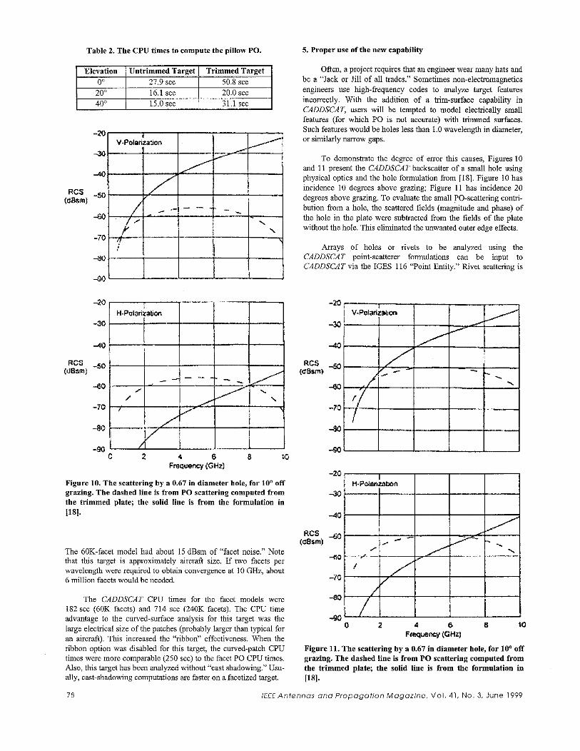
Table 2. The CPU times to compute the pillow PO.

20“

5. Proper use of the new capability

16.1 sec 20.0 sec 40’ 15.0sec

RCS (desm)

31 1 sec

-20

-30

4 0

-50

-60

- io

4 0

4 0

RCS -w

4 0

-70

40

(dBsm)

-4n

Figure 10. The scattering by a 0.67 in diameter hole, for lo0 off grazing. The dashed line is from PO scattering computed from the trimmed plate; the solid line is from the formulation in llS1.

The 60K-facet model had about 15 dBsm of “facet noise.” Note that this target is approximately aircraft size. If two facets per wavelength were required to obtain convergence at 10 GHz, about 6 million facets would be needed.

The CADDSCAT CPU times for the facet models were 182 sec (60K facets) and 714 sec (240K facets). The CPU time advantage to the curved-surface analysis for this target was the large electrical size of the patches (probably larger than typical for an aircraft). This increased the “ribbon” effectiveness. When the ribbon option was disabled for this target, the curved-patch CPU times were more comparable (250 sec) to the facet PO CPU times. Also, this target has been analyzed without “cast shadowing.” Usu- ally, cast-shadowing computations are faster on a facetized target.

Often, a project requires that an engineer wear many hats and he a “Jack or Jill of all trades.” Sometimes non-electromagnetics engineers use high-frequency codes to analyze target features incorrectly. With the addition of a trim-surface capability in CADDSCAT, users will be tempted to model electrically small features (for which PO is not accurate) with trimmed surfaces. Such features would be holes less than 1.0 wavelength in diameter, or similarly narrow gaps.

To demonstrate the degree of error this causes, Figures 10 and 11 present the CADDSCAT backscatter of a small hole using physical optics and the hole formulation from [IS]. Figure 10 has incidence 10 degrees above grazing; Figure 11 has incidence 20 degrees above grazing. To evaluate the small PO-scattering contr- bution from a hole, the scattered fields (magnitude and phase) of the hole in the plate were subtracted from the fields of the plate without the hole. This eliminated the unwanted outer edge effects.

Arrays of holes or rivets to be analyzed using the CmDSCAT point-scatterer formulations can he input to CADDSCAT via the IGES 116 “Point Entity.” Rivet scattering is

~

78 iEEEAntennas a n d Propaga t ion M o g a r i n e . Vo l . 41, No. 3. June 1999

-20

-30

-40

RCS 6 0 (a8sm)

-60

-70

-80

4 a 0 2 1 8 8 IO

FWuency (GHZ)

Figure 11. The scattering by a 0.67 in diameter hole, for 10’ off grazing. The dashed line is from PO scattering computed from the trimmed plate; the solid line is from the formulation in Wl.

described by average RCS levels, obtained from Method-Of- Moments or test data.

Electrically small gaps in surfaces are also analyzed with non-PO-based techniques. Because the gaps on a typical conven- tional aircrafl are so numerous, it is important to provide a geome- try interface to the RCS analysis that does not require re-formatting the gap data once it is received from the designer. This is accom- plished in CADDSCAT by importing the gap-space curves in the IGES format: gap position is provided via the IGES 112 and 126 space curve entities; width, depth, and treatments are also inputs (see [I]). Figure 15 fTom [I] shows a real-world FIX gap configu- ration displayed by the MrPatches code.

6. Design recommendations and restrictions

when preparing a trimmed geometry model for CADDSCAT, the following points should he taken into account.

CADDSCAT operates more efficiently when B surfaces are restricted to cubics. CADDSCAT normally converts untrimmed higher-order surfaces to cubic surfaces automatically. This auto- matic conversion is not performed for trimmed surfaces.

B-spline surfaces should be as large as possible. When many small B surfaces are used to compose a component, many of the border patches have trim lines, and thus fall into the “partially trimmed” category for which analysis is less efficient. By building up large grids of control points and building larger B surfaces, it is likely that fewer patches will be partially trimmed, and thus the entire geometry i s more efficiently analyzed.

If a switch is available, higher-order B-spline trim c w e s should be limited to cubic order. This allows the algorithms to exe- cute more efficiently.

All surface normals in the IGES file should be in the correct outward-pointing direction (i.e., pointing into the wind-stream). There is an option allowing surface-normal directions to be “ran- dom.” The option may be used for higher-bounce PO computa- tions; however, the option is not recommended for first-bounce PO (direct illumination) for low-signature targets. Thus, it is not ahsolutely necessary to modify the normal of surfaces deep in the interior of a model, such as in an inlet duct.

In order to compute edge diffraction with CADDSCAT, trims must he removed in the vicinity of the desired edges. This limita- tion will be removed in later CADDSCAT versions.

7. Conclusions

It has been demonstrated that the high-frequency physical- optics-based code CADDSCAT can utilize trimmed curved sur- faces. Validations for canonical targets were presented. A signifi- cant potential savings in design person-hours and a reduction in design cycle time has been made possible. This, in tun, allows for more alternative, innovative designs.

The CADDSCAT code is available to qualified US govem- ment requesters. It is compatible with most UNIX operating sys- tems, as well as Windows NT. To request the code, send an e-mail to james.m.roedder@boeing.com, or telephone the author at (314) 232-7083.

~

IEEEAntennas andPropagotfon Mogozfne. V o l 41. No 3. J u n e 1999 79

8. Acknowledgements

The author would like to thank Dr. John Volakis for his sug- gestions for improving this paper.

9. Notes

1. OpenGL routines could also be used to render trimmed surfaces [9]. These routines are faster than those used in MrPatches, since they utilize graphics-engine hardware and highly tuned algorithms. However, the intent here is to look at the target as the PO code sees it-not as OpenGL sees it.

2. Technically, neither CADDSCAT nor MrPatches perform “ray tracing:” they perform “ray casting.” The term “ray tracing” is primarily associated with the production of high-quality render- ings, e.g., the creation of image sequences for movies. These ren- derings require “ray tracing” to include the multiple reflections of visible light that are required for realism. The RCS community almost always uses the lerm “ray tracing” for processes that the actual ray-tracing community would call “ray casting.”

10. References

1. D. M. Elking, I. M. Roedder, D. D. Car, S. D. Alspach, “A Review of High-Frequency Radar Cross Section Analysis Capa- bilities at McDonnell Douglas Aerospace,” IEEE Antennas and Propagation Magazine, 37, 5 , October 1995, pp. 33-43.

2. “Initial Graphics Exchange Specification,” available from the National Institute of Standards and Technology (NIST).

3. J. M. Rius, M. Fenando, L. Jofre, “High Frequency RCS of Complex Radar Targets in Real Time,” IEEE Tvansnctions on Antennas and Propagation, AP-41, 9, September 1993; see also I. S. Asvestas, “The Physical Optics Integral and Computer Graph- ics,” IEEE Transactions on Antennas and Propagation, AP-43, 12, December, 1995.

4. Michael E. Mortenson, Geometric Modeling, Second Edition, New York, John Wiley, 1997, p. 146-147.

5 . A. Rockwood, K. Heaton, T. Davis, “Real-Time Rendering of Trimmed Surfaces,” SIGGRAPH ‘89 Proceedings, (July 31- Augnst4, 1989), 23, 3, p. 107-116.

6. C. deBoor, A Practical Guide to Splines, Springer-Verlag (Applied Mathematical Sciences Volume 27), 1978, p. 114.

7. D. D. Car, J. M. Roedder, “A Versatile Geometry Tool for Computational Electromagnetics: MrPatches,” Applied Conlputa- tional Elecfvomagnetic Society (ACES) Symposium Proceedings, March 1997.

8. J. M. Roedder, “GEOMPACK Programming Manual” and ”GEOMPACK Users Manual.”

9. M. Woo, J. Neider, T. Davis, OpenGL Programming Guide, Second Edition, Addison Wesley, 1997.

10. R. L. Haupt and V. V. Liepa, “Synthesis of Tapered Resistive Strips,” IEEE Transactions on Antennas and Propagation, AP-35, 11, November 1987.

11. A. S. Glassner, An Introduction to Ray Tracing, New York, Academic Press, 1989, Chapter 6: “A Survey of Ray Tracing Acceleration Techniques.”

12. The “Ray Tracing News’’ is an e-mail/WWW discussion group organized by a well known ray-tracing expert, Eric Haines. The URL for the “Ray Tracing Ncws” is http://www.acm.org/tog/resourccs/RTNcws/html/i~dcx.html.

13. J. G. Cleary, G. Wyvill, “Analysis of An Algorithm For Fast Ray Tracing Using Uniform Space Subdivision,” The Visuol Com- puter, 4, 1988, pp. 65-83.

14. A. Fujinioto, T. Tanaka, K. Iwata, “ARTS: Accelerated Ray- Tracing System,” IEEE Compuier Graphics and Animation, April, 1986, pp. 17-26.

15. H. Weghorst, G. Hooper, D. P. Greenberg, “Improved Com- putational Methods for Ray Tracing,” ACM Transactions on Graphics, 3, 1, January 1984, pp. 52-69.

16. Kevin Dowd, High Performance Computing, O’Reilly & Associates, 1993.

17. Eric Haines, “Chapter 2: Essential Ray Tracing Algorithms,” and Pat Hanrahan, “Chapter 3: A S U N C ~ of Ray-Surface Intersec- tion Algorithms,” in A. S. Glassner (ed.), An Introduction to Ray Tracing, New York, Academic Press, 1989.

18. A. K. Dominek, L. Peters, “RCS Measurement of Small Cir- cular Holes,’’ IEEE Transactions on Antennas and Propagation, AP-36, IO, October 1988, pp. 1495-1497.

EM Programmer’s Notebook

As noted by John Volakis in this issue’s EM Programmer’s Notebook, it is a great pleasure to welcome David Davidson to the Magazine Staff as a co-Associate Editor of that column. David will be primarily responsible for contributions from Asia and Europe, both accepting and soliciting contributions to the column.

David Bruce Davidson was born in London, England, in 1961. His family moved to South Africa in 1968. He was educated in South Africa, matriculating at Pretoria Boy’s High School. His BEng(1982), BEng (Hons) (1983), and MEng (1986) degrees (all cum laude) were obtained at the University of Pretoria. Following compulsory national service (1984-5) in the Signals Corps of the then SADF, he worked on computational electromagnetics at the defense electronics institute of the Council for Scientific and Industrial Research in Pretoria.

In 1988, he was appointed as a lecturer at the Department of Electrical and Electronic Engineering at the University of Stellen- bosch, where he received his PIC in 1991 for work on parallel MOM computing. He is presently a Professor in the department. He has spent sabbaticals at the University of Arizona (1993) and Cambridge University (1997), where he was a Visiting Fellow at Trinity College.

David‘s main research interests continue to focus on CEM. In addition to the above doctoral work on the MOM, he has done gen- era1 work on antenna characterization using MOM codes. He has worked with the FDTD for massively parallel systems, FSS design and material characterization. He has also been involved with the FEM, which is his main current interest. He is presently working closely with the Stellenbosch-based company Electromagnetic Software and Systems on FEM and hybrid FEM-MOM work.

David has published 27 papers on computational electromag- netics in peer-reviewed journals, and has authored or co-authored around 60 conference papers. He has advised four doctoral candi- dates and supervised ten MSc projects. He recently S C N ~ as Guest Editor for the ACES Journal‘s special issue on high-performance computing and CEM. He is a recipient of the (South African) FRD President’s Award (IEEE Antennas and Propagation Magazine, 37, 6, December 1995, p. 100). He is a member of the IEEE, ACES, and SAIEE, and is past Chair of the IEEE Joint APMTT Chapter of South Africa.

Outside electromagnetics, David has numerous interests, including tennis, squash, and mountaineering, as well as war- gaming with miniature figurines. >h‘

80 \€€€Antennas ondPropagotion Magazine. V o l . 41, No. 3, June 1999