cad/cam by munir eraghubi master of engineering - doras - dcu
TRANSCRIPT
CAD/CAM
By
Munir Eraghubi
This thesis is submitted as fulfilment of the
requirement for the award of degree of
Master Of Engineering (M. Eng) by research
to
Dublin City University
August 2004
Research Supervisor: Dr Paul Young & Prof Salecm Hashmi
School of Mechanical & Manufacturing Engineering

Declaration
1 hereby certify that this material, which I now submit for assessment on the
programme o f study leading to the award of Master o f Engineering is entirely my own
work and has not been taken from the work of others save to the extent that such work
has been cited and acknowledged within the text o f my work
S i g n e d : ______(Candidate)
ID No.:99145936
Date: August 2004
II

Acknowledgements
I would like to express my sincere thanks and gratitude to Dr Paul Young for his
excellent supervision, helpful advice and constant encouragement and guidance.
Without his support and continuous advice throughout this research it would not have
been possible to finish this thesis. 1 am honoured to have him as my supervisor for
this research.
Many thanks to professor M.S.J Hashmi for his guidance and helpful advice.
Thanks to Keith Hickey, school IT system administrator, for offering his time and
expertise when required.
Thanks to my fellow graduate students for their spontaneous support and comments.
Ill
Integration of Rapid Prototyping Technology with
CAD/CAM
By
Munir Eraghubi B. Eng
Abstract
Rapid prototyping(RP) is a relatively new technology, which still faces challenges and
a lot of problems in different stages of the process; this makes RP technology
available only using very specialised equipment and very sophisticated software. This
project is a step towards expanding the use o f this technology, easing some of the
difficulties and knowledge required to use RP systems.
Using existing CAD/CAM software, which is well understood and normally used in
machining operations the software developed manipulates the machining code from
the AlphaCAM package and generates code and instructions suitable for RP
technology.
Two user-friendly programs were developed using Visual Basic to generate control
code for a wax droplet RP system previously developed. CAD/RP follows the
traditional method in RP and generates control instructions for the system from a STL
file. The CNC/RP software is designed to generate control instructions for the system
to build a prototype from CNC code, generated using AlphaCAM. This work,
undertaken by the author, broadens the application o f layer manufacturing where
functional prototype parts are produced.
IV
TABLE OF CONTENTS
Title PageDECLARATION II
ACKNOWLEDGEMENTS III
ABSTRACT IV
TABLE OF CONTENTS V
LIST OF FIGURES XI
Chapter 1 Introduction 1
Chapter 2 Overview O f Rapid Prototyping 3
2.1 Model Generation 3
2.2 3D Model Transfer 4
2.3 Process Planning 6
2.4 Overview of RP Technologies 9
2.5 Applications 22
2.6 Development in RP 23
2.7 Computer Aided Design (CAD) 28
2.8 Computer Aided Manufacturing (CAM) 28
2.9 Computer Aided Design And Manufacturing CAD/CAM 29
2.10 Principle of Numerical Control 30
Chapter 3 Overview of the Wax Droplet RP System 34
3.1 Deposition system 34
3.2 Precision manipulator 35
3.3 Wax RP system operation 36
3.4 Elements of control 36
3.5 X Language and position modes 38
Chapter 4 Development o f The System 40
4.1 Development of CAM/RP software 42
4.2 Development of CAD/RP software 44
V
4.3 Introduction of using CAD/CAM for RP 62
4.4 Development of CNC/RP software 69
Chapter 5 Result And Discussion 86
5.1 CAD/RP 865.2 CNC/RP 93
5.3 Result of Wax Droplet RP System 99
Chapter 6 Conclusion and Suggested Future Work 105
6.1 Advantages Of Using CAD/CAM For RP. 105
6.2 Thesis Contribution 106
6.3 Suggested Future Work 107
References 112
Appendix A Preparatory codes [59] 119
Appendix B Command Listing [53] 122
Appendix C CAD/RP Algorithms 125
Appendix D CNC/RP Algorithms 138
Appendix F CAM/RP Algorithms 159
VI

LIST OF FIGURES
Title Page
Figure 1 The Basic Technique of Rapid Prototyping 3
Figure 2 Example of STL file and description format ASCII representation 5
Figure 3 Example of many objects in STL format [] 5
Figure 4 The effect o f slicing with different layer thickness on the
produced part accuracy 6
Figure 5 Three type of tolerance distribution while slicing 7
Figure 6 ACES build style 8
Figure 7 STAR WEAVE build style 8
Figure 8 Quick Cast build styles 9
Figure 9 Classification of rapid prototyping methods (adapted from [3,7] ) 10
Figure 10 Schematic of stereolithography (SLA) RP process. 11
Figure 11 Schematic of selective laser sintering (SLS) RP process 13
Figure 12 Schematic of Laminated Object Manufacturing (LOM) 15
Figure 13 Schematic o f Three-Dimensional Printing (3D Printing) 17
Figure 14 Fused Deposition Modelling (FDM) 18
Figure 15 Ballistic Particle Manufacturing (BPM) 20
Figure 16 Chordal error between actual surface and tessellated surface 24
Figure 17 The stair-step effect due to layer thickness. 24
Figure 18 Methods o f slicing to reduce the staircase errors 25
Figure 19 CNC program generated in AlphaCAM software 31
Figure 20 Illustration of variables used in circular interpolation 33
Figure 21 Wax Droplet RP System 34
Figure 22 The components of the deposition system 35
Figure 23 Picture of Precision x-y manipulator system 36
Figure 24 Interface Systems between the PC and the motors. 37
Figure 25 Flow diagram for RP operation 40
VII

Figure 26 X language commands Output from CAD/RP and CNC/RP 41
Figure 27 Structure of the developed CAD/RP program 44
Figure 28 Start-up screen 45
Figure 29 File open dialogue box in the CAD/RP program. 45
Figure 30 View menu of CAD/RP program 46
Figure 31 Position mode set-up dialogue box 48
Figure 32 Axis Set-up dialogue box 48
Figure 33 Motor speed set-up dialogue box 49
Figure 34 Process Set-up dialogue box 50
Figure 35 Run menu for CAD/RP program 50
Figure 36 Run algorithm flow chart 51
Figure 37 The possible cases examined for facet-plane slicing in the
CAD/RP program. 52
Figure 38 Three vertices o f one triangle and the intersection points 53
Figure 39 Slicing algorithm flow chart for CAD/RP program 54
Figure 40 Contour sorting 55
Figure 41 Contour construction algorithm flow chart for CAD/RP program. 55
Figure 42 Contour filling point selection illustration. 56
Figure 43 Flow chart for the contour-filling algorithm 57
Figure 44 Flow chart for simulation algorithm 58
Figure 45 Delay form for CAD/RP 60
Figure 46 Save common dialogue box 61
Figure 47 Generate CNC code for RP from AlphaCAM 63
Figure 48 Tool Directions form in AlphaCAM software 64
Figure 49 Pocketing forml in AlphaCAM software 65
Figure 50 Pocketing form 2 in AlphaCAM software 65
Figure 51 Linear Pocket Sides Vertical form in AlphaCAM software 66
Figure 52 Linear Pocket - Tool: Flat 3mm 2F EC HSS form in
AlphaCAM software 67
Figure 53 Tool Path Result for the rectangular 68
Figure 54 Output NC.form 68
VIII
Figure 55 Structure of the CNC/RP program 69
Figure 56 Start-up screen 70
Figure 57 Import command. 70
Figure 58 View menu 71
Figure 59 Indexer set-up form in CNC/RP program. 72
Figure 60 Rum menu 73
Figure 61 CNC/RP run algorithm flow chart 74
Figure 62 Extract algorithm flow chart 75
Figure 63 Define Circular interpolation for PC23 76
Figure 64 Circular interpolation 78
Figure 65 The four cases for circular interpolation 79
Figure 66 AO problem 80
Figure 67 flow chart to find the right centre for the interpolation 81
Figure 68 chord length for one step angle 82
Figure 69 CNC/RP simulation algorithm 83
Figure 70 Error due to moving from fabricated point 84
Figure 71 Starting the new movement from the original last position 84
Figure 72 Various views for the imported design in CAD/RP. 87
Figure 73 Construction of contour as found in STL file 88
Figure 74 Construction of contour as found in STL file 89
Figure 75 Raster scan pattern filling 90
Figure 76 Building the contour 91
Figure 77 Building the cross-section area 91
Figure 78 Instruction command for CAD/RP 92
Figure 79 Drawing the CNC tool path for different parts 94
Figure 80 Simulating the deposition of wax 95
Figure 81 Figure 81 Voids and Geometric Errors 96
Figure 82 The simulation before and after correcting the tool path 97
Figure 83 The simulation after correcting the tool path 97
Figure 84 Filtering operation with different factors 98
Figure 85 Motion code for the PC23 98
IX
Chapter 1 Introduction
Until recently, prototypes were still constructed by skilled craftsmen from 2D
drawings, adding weeks or months to the product development time. Currently
product design is becoming more complex, while the need for reducing the time to
market has increased.
CAD/CAM technology has provided a new way to produce accurate parts directly
from CAD models in a few hours for a fraction of manufacturing cost, with little need
for human intervention.
While there are a number of vendors using different technologies in their particular
equipment, most o f the additional RP systems work under the same fundamental
principals. This consists of 3D CAD data, in a specific file format usually (STL),
oriented in an optimal build position and direction, the file is then sliced numerically
into layers representing horizontal cross-sections of the part. The RP machine then
fabricates each layer and bonds it to the previous layer, starting from the bottom
section and working up to the top until the part is complete [1,2],
This technology allows companies to produce physical models o f their designs more
often, allowing them to check the assembly and function of a design while spending
less time and money. It has been claimed that RP can cut the cost of developing new
products by up to 70%, and the time to market by 90% [3,4],
Rapid prototyping is a relatively new technology, which is still facing a lot of
problems in different stages of the process; this makes RP technology available only
using specialised equipment and specialist trained staff. This project is a step towards
spreading this technology and to ease some of the difficulties by using existing
CAD/CAM software, which is commonly used in machining operations, through the
introduction of a software package, to manipulate the CNC code and generate
instructions suitable for RP.
The developed software scans the CNC code, which is generated using AlphaCAM,
manipulates the tool path, simulates the deposition of wax, filtering deposition of
excess material in some areas, and then translates the CNC code to X-language codes,
which are the PC23 indexer instructions to drive the motors. To prove the
effectiveness o f the solution some examples were built using this strategy and a wax
droplet RP system previously developed in DCU.
The wax droplet RP system consists of a heated cylinder containing the wax and a
plunger head fitted in the cylinder to increase the pressure inside the cylinder. Then
this deposits one drop then retracts to hold the wax inside the cylinder. An indexer is
used to drive the three motors, two motors to provide the X-Y movement while a third
is to deposit the wax. The indexer receives the instructions from a personal computer
in a special instruction set called X-language.
This approach can solve many problems at different stages of the rapid prototyping
process, such as data transfer, slicing the geometry, tool path generation, building the
support structure and fabricating multiple materials. The work undertaken by the
author contributes specially to layer manufacturing where functional parts are
produced and more control over the building operation is needed. As in the material
removal technologies, where engineers control the machining operation and generate
the CNC code to create different features on the part using a range o f tools that are
available for machining operations, addition technologies are now more controllable
by varying the operation parameters. These parameters include as the layer thickness,
the deposition diameter in some technologies or the laser beam within other
technologies, the travel speed and touch angle. This is not only for the whole
operation, but it could be varied for each feature to achieve the required property,
especially when a large number of the product is needed.
2
Chapter 2 Overview Of Rapid Prototyping
Rapid Prototyping (RP) refers to fabrication of parts layer-by-layer. It involves adding
raw material successively, in layers, to create a solid of a predefined shape. The
process is fully automatic and it offers many advantages over traditional
manufacturing processes.
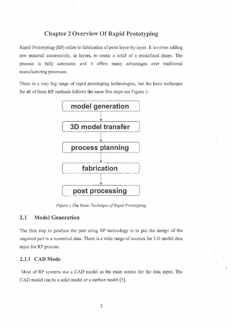
There is a very big range of rapid prototyping technologies, but the basic technique
for all o f these RP methods follows the same five steps see Figure 1:
Figure 1 The Basic Technique o f Rapid Prototyping
2.1 Model Generation
The first step to produce the part using RP technology is to put the design o f the
required part in a numerical data. There is a wide range o f sources for 3-D model data
input for RP process.
2.1.1 CAD Mode
Most o f RP systems use a CAD model as the main source for the data input. The
CAD model can be a solid model or a surface model [5].
3
A solid model is a complete mathematical representation of the shape o f a physical
object, it contains two types of data to describe the part, geometric data and
topological data. Geometric data defines the basic shape, lines, curves, and surfaces.
The topological data contains the connectivity relationship among the geometric
components and allows the computer to determine the volume that is enclosed by the
object’s surfaces. There are many types o f solid modellers in use, the most commonly
used are: Constructive solid geometry, Boundary representation (B-rep), and
Polyhedral modelling [2, 6].
A surface model defined by a number o f surfaces with zero thickness is joined
together to form the part. Since there is no topological data to define association
between these surfaces, it is possible to have gaps or even missing surfaces. The
surface model has to have a closed surface for use in rapid prototyping [6, 7].
2.1.2 Reverse engineering data
Reverse Engineering is the process of recreating an engineering design data from
existing parts by acquiring the surface data using a laser scanning system, contact
probe, digitisers, or computer vision. This technique is very useful when the
engineering design is lost or when the physical model has gone through many design
changes [8, 9, 10, 11].
2.2 3D Model Transfer
To fabricate any design in current rapid prototyping systems the 3-D model (surface
or solid) has to be transferred to STL (standard transform language)[12] format, which
is the most common standard interface between CAD and RP systems [1].
STL format was developed and published in 1987 by 3D systems for converting 3D
CAD models for use in stereolithography and has become the de-facto standard for
the data input for all types o f RP systems [1,2].
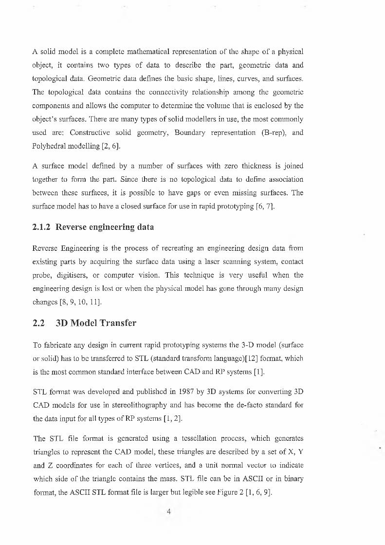
The STL file format is generated using a tessellation process, which generates
triangles to represent the CAD model, these triangles are described by a set of X, Y
and Z coordinates for each of three vertices, and a unit normal vector to indicate
which side of the triangle contains the mass. STL file can be in ASCII or in binary
format, the ASCII STL format file is larger but legible see Figure 2 [1, 6, 9].
solid BOX -------- ------------------------------- ------— ..... ..... —(1)facet normal -1.00000000E+000 O.OOOOOOOOE+OOO O.OOOOOOOOE+OOO —(2)
outer loop -------------------------------------------------------------------(3)vertex-3.90508985E+001 4.27599077E+001 2.27695819E+001 vertex-3.90508985E+001 4.27599077E+001 -2.23041810E+000 —(4)vertex-3.90508985E+001 6.16805593E+000 -2.23041810E+000
endfacet -------------------------------------------------------------------(6)facet normal -1.00000000E+000 O.OOOOOOOOE+OOO O.OOOOOOOOE+OOO
outer loopvertex-3.90508985E+001 6.16805593E+000 -2.23041810E+000 vertex-3.90508985E+001 6.16805593E+000 2.27695819E+001 vertex-3.90508985E+001 4.27599077E+001 2.27695819E+001
endloop endfacet
endsolid BOX ----- ---- ----------------------------------------------------- (7)
(1) The start of solid(2) Identifies the material side(3) The start of the triangle vertex(4) x, y, z for each vertex
(5) End of the triangle vertex(6) End of the triangle information(7) End of the solid information
Figure 2 Example o f STL file and description format ASCII representation
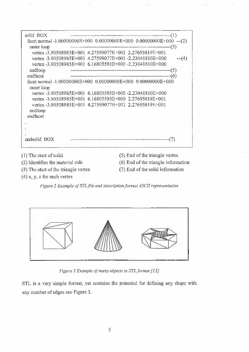
Figure 3 Example o f many objects in STL format [13]
STL is a very simple format, yet contains the potential for defining any shape with
any number of edges see Figure 3.
5
2.3 Process Planning
Process planning is a stage where the control instructions are generated and the
process parameters are selected, at this stage the system and the operator carry out the
following steps.
2.3.1 Select an orientation
An optimal build direction has to be determined to improve part accuracy, the surface
finish, assessing the need for support structures and to reduce the production time,
which leads to minimizing the cost of producing the prototype [14, 15, 16],
2.3.2 Create supports
Some models have overhanging portions, which need support structures to build it.
Some RP systems do not need to build support structures, where uncured material
works as a support structure [5],
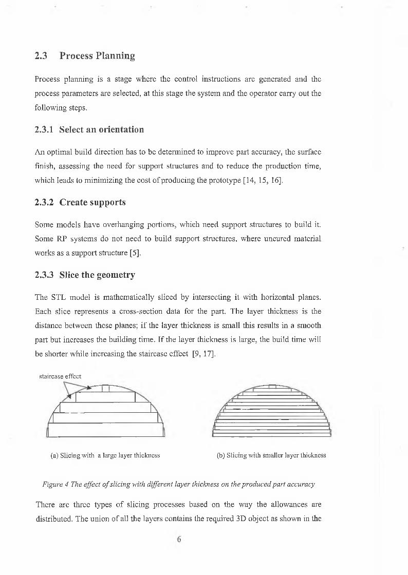
2.3.3 Slice the geometry
The STL model is mathematically sliced by intersecting it with horizontal planes.
Each slice represents a cross-section data for the part. The layer thickness is the
distance between these planes; i f the layer thickness is small this results in a smooth
part but increases the building time. If the layer thickness is large, the build time will
be shorter while increasing the staircase effect [9, 17].
staircase effect
I/
(a) Slicing with a large layer thickness (b) Slicing with smaller layer thickness
Figure 4 The effect o f slicing with different layer thickness on the produced part accuracy
There are three types of slicing processes based on the way the allowances are
distributed. The union of all the layers contains the required 3D object as shown in the
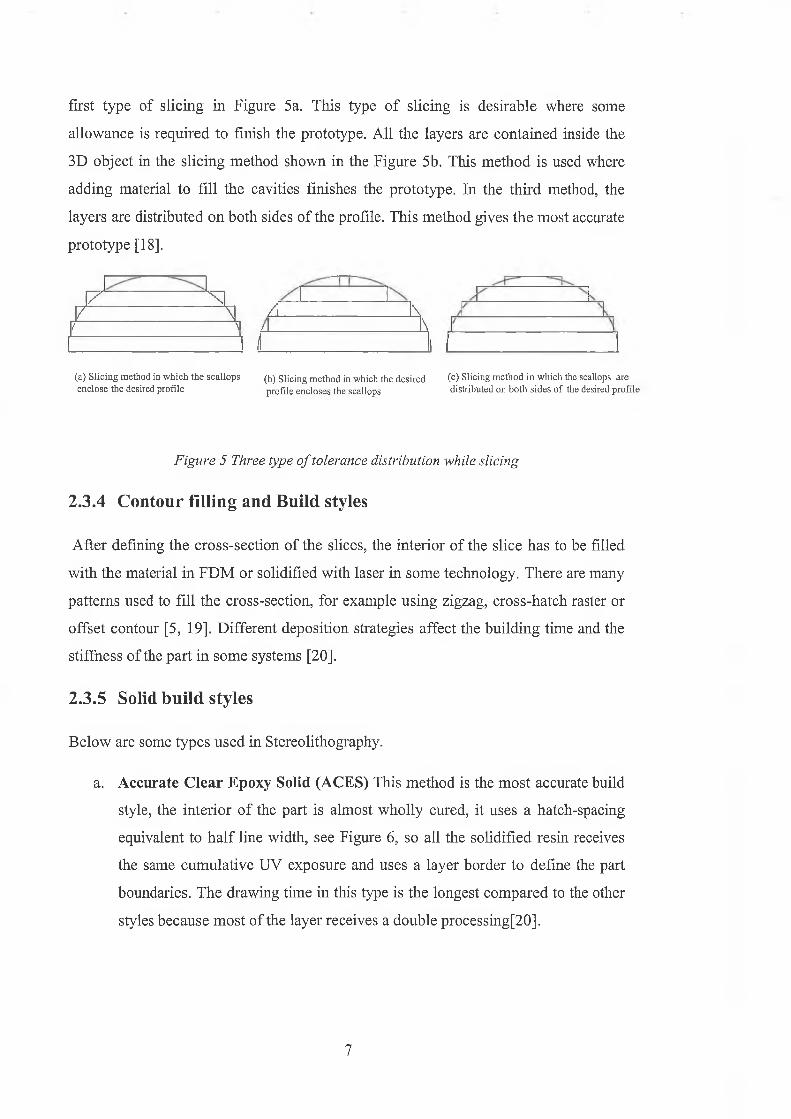
first type of slicing in Figure 5a. This type o f slicing is desirable where some
allowance is required to finish the prototype. All the layers are contained inside the
3D object in the slicing method shown in the Figure 5b. This method is used where
adding material to fill the cavities finishes the prototype. In the third method, the
layers are distributed on both sides of the profile. This method gives the most accurate
prototype [18].
y x/ \ / \f --------- Y / \
1 (i 1 1(a) Slicing method in which the scallops (b) Slicing method in which the desired (c) Slicing method in which the scallops areenclose the desired profile profile encloses the scallops distributed on both sides o f the desired profile
Figure 5 Three type o f tolerance distribution while slicing
2.3.4 Contour filling and Build styles
After defining the cross-section of the slices, the interior of the slice has to be filled
with the material in FDM or solidified with laser in some technology. There are many
patterns used to fill the cross-section, for example using zigzag, cross-hatch raster or
offset contour [5, 19]. Different deposition strategies affect the building time and the
stiffness of the part in some systems [20].
2.3.5 Solid build styles
Below are some types used in Stereolithography.
a. Accurate Clear Epoxy Solid (ACES) This method is the most accurate build
style, the interior of the part is almost wholly cured, it uses a hatch-spacing
equivalent to half line width, see Figure 6, so all the solidified resin receives
the same cumulative UV exposure and uses a layer border to define the part
boundaries. The drawing time in this type is the longest compared to the other
styles because most of the layer receives a double processing[20].
7
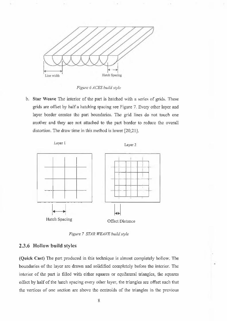
Figure 6 ACES build style
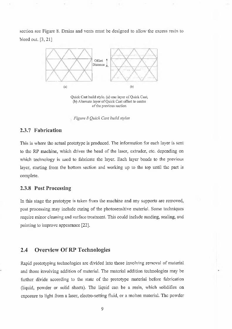
b. S tar W eave The interior of the part is hatched with a series of grids. These
grids are offset by half a hatching spacing see Figure 7. Every other layer and
layer border creates the part boundaries. The grid lines do not touch one
another and they are not attached to the part border to reduce the overall
distortion. The draw time in this method is lower [20,21],
Layer 1 Layer 2
Hatch Spacing Offset Distance
Figure 7 STAR WEA VE build style
2.3.6 Hollow build styles
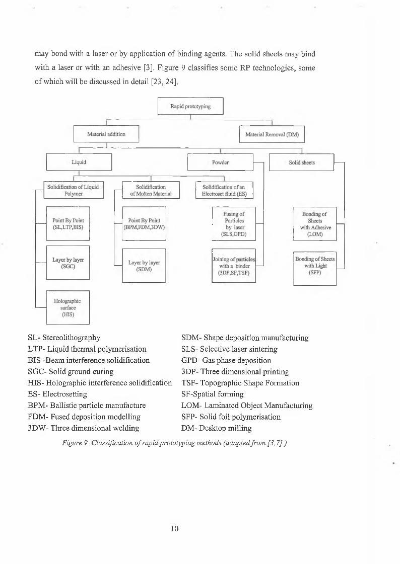
(Q uick Cast) The part produced in this technique is almost completely hollow. The
boundaries o f the layer are drawn and solidified completely before the interior. The
interior of the part is filled with either squares or equilateral triangles, the squares
offset by half of the hatch spacing every other layer, the triangles are offset such that
the vertices of one section are above the centroids of the triangles in the previous
8
section see Figure 8. Drains and vents must be designed to allow the excess resin to
bleed out. [3, 21]
I
(a)
Quick Cast build style, (a) one layer of Quick Cast;(b) Alternate layer of Quick Cast offset to centre
of the previous section
Figure 8 Quick Cast build styles
2.3.7 Fabrication
This is where the actual prototype is produced. The information for each layer is sent
to the RP machine, which drives the head of the laser, extruder, etc. depending on
which technology is used to fabricate the layer. Each layer bonds to the previous
layer, starting from the bottom section and working up to the top until the part is
complete.
2.3.8 Postprocessing
In this stage the prototype is taken from the machine and any supports are removed,
post processing may include curing o f the photosensitive material. Some techniques
require minor cleaning and surface treatment. This could include sanding, sealing, and
painting to improve appearance [22].
(b)
2.4 Overview Of RP Technologies
Rapid prototyping technologies are divided into those involving removal o f material
and those involving addition of material. The material addition technologies may be
further divide according to the state o f the prototype material before fabrication
(liquid, powder or solid sheets). The liquid can be a resin, which solidifies on
exposure to light from a laser, electro-setting fluid, or a molten material. The powder
OffsetDistance
9
may bond with a laser or by application of binding agents. The solid sheets may bind
with a laser or with an adhesive [3]. Figure 9 classifies some RP technologies, some
of which will be discussed in detail [23, 24],
SL- StereolithographyLTP- Liquid thermal polymerisationBIS -Beam interference solidificationSGC- Solid ground curingHIS- Holographic interference solidificationES- ElectrosettingBPM- Ballistic particle manufactureFDM- Fused deposition modelling3DW- Three dimensional welding
SDM- Shape deposition manufacturing SLS- Selective laser sintering GPD- Gas phase deposition 3DP- Three dimensional printing TSF- Topographic Shape Formation SF-Spatial formingLOM- Laminated Object Manufacturing SFP- Solid foil polymerisation DM- Desktop milling
Figure 9 Classification o f rapid prototyping methods (adapted from [3,7] )
10

2.4.1 Stereo lithography (SLA)
Stereolithography is considered the most popular RP technology. It was first invented
by Charles Hull [6] and introduced commercially in 1988 by 3D systems. The
material used is a photosensitive liquid resin (epoxy) [3], which when exposed to an
ultra - violet helium-cadmium or argon ion laser forms a polymer and solidifies.
The SLA machine consists of a platform, which is mounted in a vat o f resin, see
Figure 10. The platform is lowered below the surface o f the resin by a layer thickness.
The laser beam traces the contour o f the layer, then the cross section o f the model is
either hatched or solidified using information obtained from the 3D solid model. Once
a layer is completed, the platform is lowered a layer thickness, which is defined by the
depth limit of the light absorption [6]. The resin flows over the first layer, and is left
until it settles. In some machines a wiper is used to spread the viscous polymer. The
laser draws a new layer on top o f the previous layer, this process continues until the
part is completed.
Lasersource
Figure 10 Schematic o f stereolithography (SLA) RF process.
When the layers are finished, the part is removed from the vat drained and washed.
This may take several hours due to the resin viscosity. The supports are removed and
Mirror
Laser
Recoater Blade
Supports
PlatformLiquidphotopolymerresin
l i

the part placed in a fluorescent oven where UV light floods the prototype to
completely solidify it.
Advantages
1. The SLA machines are the most accurate machines among all current rapid
prototyping machines with an accuracy of ± 100 /xm. The 3D Systems
introduced SLA 7000 system, which has a minimum layer thickness o f 25.4
jum [6, 23, 24],
2. The model fabricated with SLA is ideal for assembly testing, function testing,
visual aids, medical models and patterns for tooling.
Disadvantages
1. The material is expensive, smelly, and toxic.
2. The material must be shielded from light to avoid premature polymerisation.
3. The part may be brittle and not strong enough for high stress testing.
4. Support structures must be built for over hanging features.
2.4.2 Selective laser sintering (SLS)
The SLS was developed by Carl Deekars and Joseph Beaman at the mechanical
engineering department of the University of Texas at Austin, and introduced to the
commercial world in 1992 by DTM Corp [6], In the first quarter of 2001, 3D system
announced the acquisition of DTM Corporation [23].
The process starts with a thin layer of powder spread across the platform using a
counter-rotating roller, and preheated to a temperature slightly below its melting point
see Figure 11. The powder is sintered using a carbon dioxide (CO2) laser of power in
the range of 25-50 W, the laser beam traces the cross section on the powder surface to
sinter the material. Then the platform is lowered and the powder feed chamber rises.
The counter-rotating roller spreads a new layer of powder. The laser draws the new
layer on top o f the previous one. The sintered powder forms the part whilst the
unscanned powder remains in place to support the next layer. This continues until the
part is completed.
12

Scanning system
C02 LaserA
Temperature controlled build chamber
Powder feed
powder
Powder leveling roller
Figure 11 Schematic o f selective laser sintering (SLS) RP process
Advantages:
1. A wide range o f material is available for this process. Including polycarbonate,
PVC (Polyvinyl chloride), ABS (acrylonirile butadiene styrene), nylon, resin,
polyropane, polyurethane, investment casting wax, sand ceramic and metals
[3,6]
2. No post curing is required (except for some materials such as ceramics).
3. No support structures are needed.
4. The materials are cheaper than the material for SLA.
5. The materials are non toxic and safe as used in this process.
6. The process is considered fast compared with SLA.
7. It produces good visual representation models.
Disadvantages:
1. Parts need a long cooling cycle.
2. Each materials has its own melting point and specific heat, so the laser
parameters need a different setting for each material.
13

3. Although this process is able to produce metallic parts the performance and
accuracy are poor due to shrinkage o f metal powder [25],
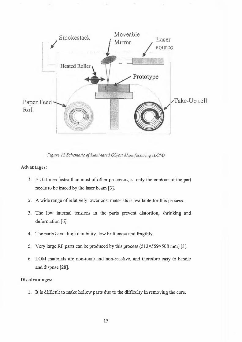
2.4.3 Laminated Object Manufacturing (LOM)
This system uses a roll of material which is drawn from a feed roller to a take-up
roller across the top of build stage see Figure 12. The material delivery rollers stop
while the material is bound to the previous layer using a hot roller, which activates a
heat-sensitive adhesive. The contour of the cross-section is then cut with a laser beam
that is carefully modulated to penetrate to a depth of exactly one layer thickness [3].
The excess material is cut into small rectangles and remains in place to support the
next layer. The build stage drops down by a layer thickness and the material is
advanced by the roller until a new layer may be cut. The width of the part is limited
by the material width.
The system uses a 25-50 W CO2 laser to cut the material, the process generates
considerable smoke so the build chamber must be sealed and either a chimney or a
charcoal filtration is required [26].
The waste material which has bonded to the part on the top and the bottom surface
must be hatched with smaller hatches to facilitate removal, it may be necessary to stop
the process to remove the material from cavities, which are too difficult to access after
completing the part. It can be time consuming to remove extra material for some
geometries.
Although the principal commercial provider o f LOM systems, Helisys, ceased
operation in 2000, Cubic Technology has been founded to support the technology, and
there are several other companies providing similar technologies. A knife is some
times used to cut the outline o f the part and cross-hatch the waste material. Ability to
bond only the required cross-section to the previous layer is used in some systems. A
new online de-cubing laminated object manufacturing process can remove about 30-
80% waste material during the machining process proposed [27], this process shortens
the time for laser cutting and de-cubing and enables the automated production of
hollow and shell-shaped parts.
14
Smokestack Moveable
n /I Mirror Laser
source
Paper FeedRoll
^/T ake-U p roll
Figure 12 Schematic o f Laminated Object Manufacturing (LOM)
Advantages:
1. 5-10 times faster than most o f other processes, as only the contour o f the part
needs to be traced by the laser beam [3].
2. A wide range o f relatively lower cost materials is available for this process.
3. The low internal tensions in the parts prevent distortion, shrinking and
deformation [6].
4. The parts have high durability, low brittleness and fragility.
5. Very large RP parts can be produced by this process (513x559x508 mm) [3].
6. LOM materials are non-toxic and non-reactive, and therefore easy to handle
and dispose [28].
Disadvantages:
1. It is difficult to make hollow parts due to the difficulty in removing the core.
15
2. The part accuracy is limited due to the comparably simple machine design
[28],
3. There is a large amount of scrap.
4. There is a fire hazard, because of using the laser for cutting the material,
which means that the machines need to be fitted with an inert gas extinguisher.
5. Finishing and sealing the parts is difficult and requires much effort [28],
6. If the part is made of paper it should be sealed with a urethane, silicone or
epoxy spray to prevent later distortion, due to water absorption.
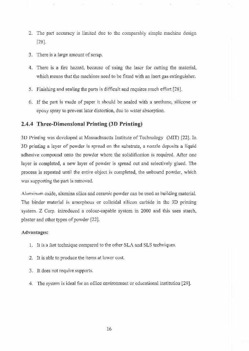
2.4.4 Three-Dimensional Printing (3D Printing)
3D Printing was developed at Massachusetts Institute o f Technology (MIT) [22]. In
3D printing a layer o f powder is spread on the substrate, a nozzle deposits a liquid
adhesive compound onto the powder where the solidification is required. After one
layer is completed, a new layer of powder is spread out and selectively glued. The
process is repeated until the entire object is completed, the unbound powder, which
was supporting the part is removed.
Aluminum oxide, alumina silica and ceramic powder can be used as building material.
The binder material is amorphous or colloidal silicon carbide in the 3D printing
system. Z Corp. introduced a colour-capable system in 2000 and this uses starch,
plaster and other types o f powder [22].
Advantages:
1. It is a fast technique compared to the other SLA and SLS techniques.
2. It is able to produce the items at lower cost.
3. It does not require supports.
4. The system is ideal for an office environment or educational institution [29].
16

r LiquidAdhesiveSupplyPowder
InjectHead \leveling
roller
PowderdeliverySystem
FabricationPiston
Figure 13 Schematic o f Three-Dimensional Printing (3D Printing)
Disadvantages:
1. The part may be fragile and porous.
2. It can be hard to remove the excess powder from the cavities.
3. A smaller stair-stepping effect in the x-y plane as well as in z direction due to
employing raster-scanning for the print head [3]
2.4.5 Fused Deposition Modelling (FDM)
Stratasya Inc. developed the FDM system, and introduced it in 1990 [6]. The system
consists o f a build platform, movable extrusion nozzle, and a control system, see
Figure 14. The extruded material is heated in the nozzle to 0.5 °C above its melting
point by a resistance heater. The nozzle traces the two-dimensional cross section of
the model and extrudes the material under the control of a precision pump [6]. The
material solidifies about 0.1 s after extrusion and cold-welds to the previous layers.
The temperature of the previous layer has to be maintained just below the melting
point of the material for good adhesion with the next layer [30], After one layer is
finished, the extrusion head moves up a layer thickness to build the next layer.
17
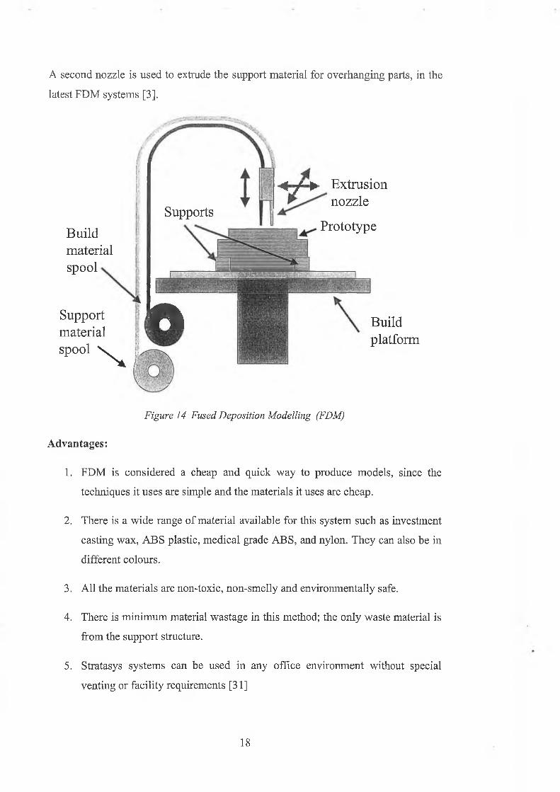
A second nozzle is used to extrude the support material for overhanging parts, in the
latest FDM systems [3].
Build material spool
Support 1 ^ ^ material spool V
4 f ► Extrusion nozzle
PrototypeSupports
Buildplatform
Figure 14 Fused Deposition Modelling (FDM)
Advantages:
1. FDM is considered a cheap and quick way to produce models, since the
techniques it uses are simple and the materials it uses are cheap.
2. There is a wide range of material available for this system such as investment
casting wax, ABS plastic, medical grade ABS, and nylon. They can also be in
different colours.
3. All the materials are non-toxic, non-smelly and environmentally safe.
4. There is minimum material wastage in this method; the only waste material is
from the support structure.
5. Stratasys systems can be used in any office environment without special
venting or facility requirements [31]
18

Disadvantages:
The main disadvantages are that the accuracy o f the part is restricted due to the shape
of the extrusion used. A typical commercial machine has accuracy of ±127 fim and
178-365 fim layer thickness [31].
2.4.6 Ballistic Particle Manufacturing (BPM)
The (BPM) technique developed by Perception Systems injects tiny droplets of
molten material from a nozzle, which hit the substrate and immediately cold-weld to
the previous layer, the injection head moves and drops the material where it is
required to form the layer o f the object [6].
The stream of molten material is separated into droplets using a drop-on-demand
system or a continuous jet. When a continuous jet is adopted, the material is injected
through the nozzle, which is being excited by a piezoelectric transducer at a frequency
of about 60Hz. The transducer must be located at a distance from the nozzle to avoid
any damage. The disturbance at the nozzle produces a stream of small, regular
droplets with uniform spacing and distance [3].
Solidscape, Inc. machine passes a milling head over the layer to make it a uniform
thickness. Particles are vacuumed away as the milling head cuts. If a clog is detected,
the jetting head is cleaned, the problem layer is milled off and then the process
continued [26],
The Thermojet machine developed by 3D systems is a much faster operation since it
deposits materials from hundreds of jets. This machine uses the modelling material
itself as support, in a very fine structure, to remove this support they are simply
brushed away[26].
Perception Systems Inc.machines use wax, Automated Dynamics Co. uses aluminum
[6], Other materials currently employed are tin, zinc, lead, lower than 420 °C melting
point alloys and thermoplastics [3].
19
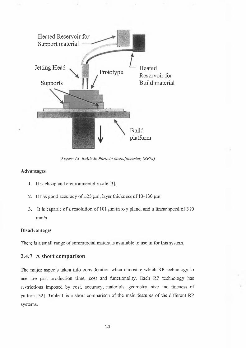
Jetting Head
Supports
Prototype Heated Reservoir for Build material
Buildplatform
Heated Reservoir for Support material
Figure 15 Ballistic Particle Manufacturing (BPM)
Advantages
1. It is cheap and environmentally safe [3].
2. It has good accuracy of ±25 /xm, layer thickness of 13-130 /xm
3. It is capable of a resolution of 101 /zm in x-y plane, and a linear speed of 310
mm/s
Disadvantages
There is a small range of commercial materials available to use in for this system.
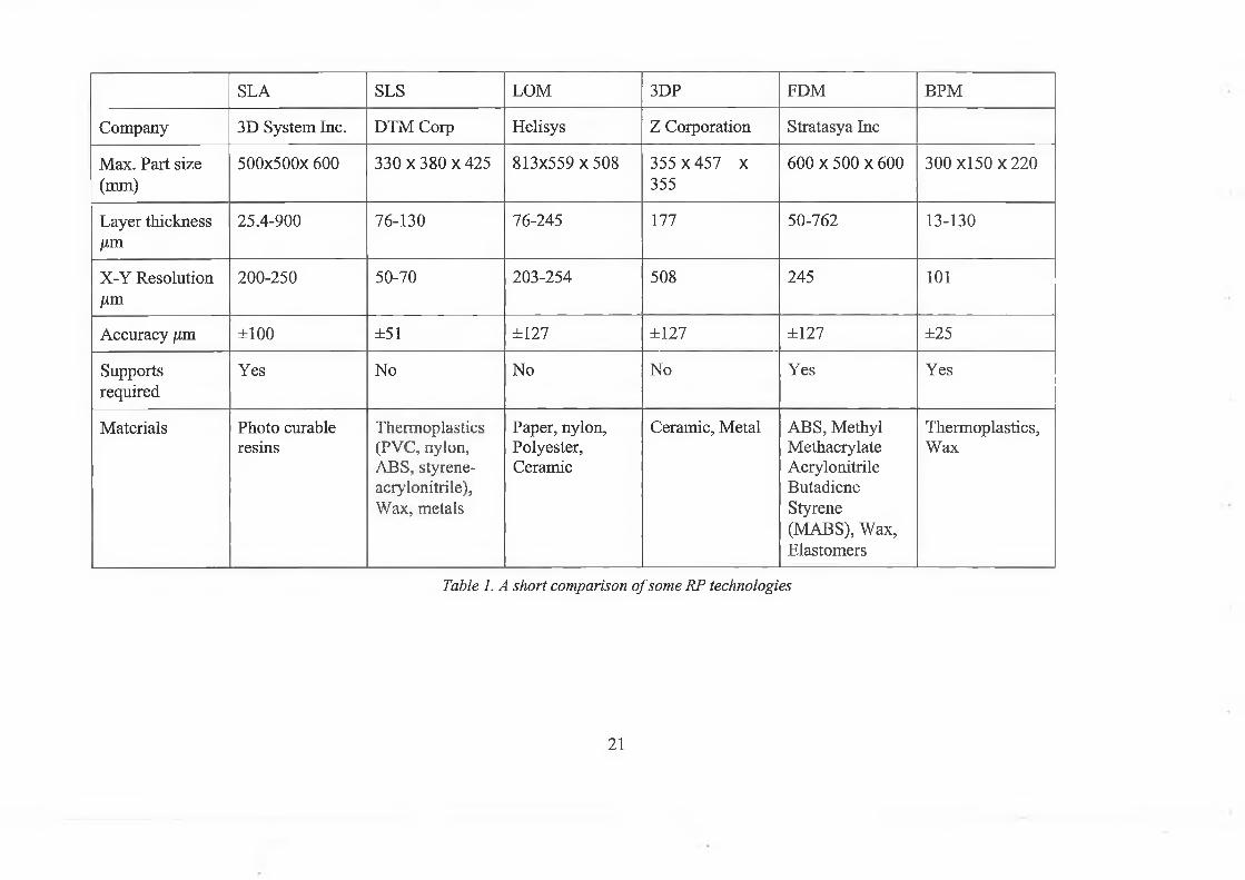
2.4.7 A short comparison
The major aspects taken into consideration when choosing which RP technology to
use are part production time, cost and functionality. Each RP technology has
restrictions imposed by cost, accuracy, materials, geometry, size and fineness of
pattern [32]. Table 1 is a short comparison of the main features of the different RP
systems.
20
SLA SLS LOM 3DP FDM BPM
Company 3D System Inc. DTM Corp Helisys Z Corporation Stratasya Inc
Max. Part size (mm)
500x500x 600 3 3 0 x 3 8 0 x 4 2 5 813x559 x508 355 x457 x 355
600 x 500 x 600 300 X150 x 220
Layer thickness [im
25.4-900 76-130 76-245 177 50-762 13-130
X-Y Resolution [in1
200-250 50-70 203-254 508 245 101
Accuracy /xm ±100 ±51 ±127 ±127 ±127 ±25
Supportsrequired
Yes No No No Yes Yes
Materials Photo curable resins
Thermoplastics (PVC, nylon, ABS, styrene- acrylonitrile), Wax, metals
Paper, nylon,Polyester,Ceramic
Ceramic, Metal ABS, MethylMethacrylateAcrylonitrileButadieneStyrene(MABS), Wax, Elastomers
Thermoplastics,Wax
Table 1. A short comparison o f some RP technologies
21
2.5 Applications
Although RP technologies are still at their early stage, a number of industrial
companies have benefited from applying these technologies to improve their product
development.
2.5.1 Verification and optimisation the Design
No matter how well engineers interpret the design concepts in CAD systems, it is still
very difficult to visualize exactly what the actual complex products will look like.
Some errors may still escape from the review of engineers and designers, with RP the
prototype can be built quickly and cheaply, therefore engineers can evaluate a design
very quickly.
2.5.2 Layer manufacturing
Making patterns for injection moulding is an expensive operation and, when small
quantities are required, it is possible to use RP technologies as a manufacturing
technique to reduce the cost and the time. In some cases parts need to be produced
with internal shapes that could not be manufactured using traditional technologies. RP
can be a solution in these cases [3].
2.5.3 Rapid tooling
It is possible to use some RP technologies to produce tools directly. RP parts are used
as moulds for concrete, fibreglass and expanding foams. Parts made of wax or other
low melting point materials may be painted with metal. The metal shells can be used
for plastic injection moulding [3], RP is used also for investment casting, where the
parts are coated with a ceramic slurry and then burnt out. When the investment casting
wax is burnt out, this leaves a very little ash content less then 0.002% while parts
made of paper in the LOM technique leave approximately 3% ash at 760 °C.
2.5.4 Marketing
Prototypes can be used to demonstrate the design concept to gain customer feed back
so that the final product will meet the customers requirements [6],
22
2.5.5 Other Applications
RP technology has been introduced successfully in the industries of automotive,
aerospace, shipbuilding, computer, toy, and consumer products. Microelectronic-
mechanical systems and medical applications are also very important fields. [33].
2.6 Development In RP
The current and future primary efforts are to manufacture "functional components"
and the "form/fit" parts that the majority of today's RP technologies produce. For this
purpose RP processes are being developed with emphasis on materials, tolerance,
software, and better process control. Many limitations associated with the RP process
have been improved in recent years with the development of new materials.
2.6.1 Accuracy
There is an increasing requirement to improve the RP part accuracy to the equivalent
o f those produced by traditional machining methods. Surface accuracy can be defined
as the deviation o f the geometry from the progenitor CAD model to the part. The loss
o f accuracy is mainly due to (1) pre-process errors, (2) process planning errors, (3)
Process errors, and (4) post-process errors [15]. These errors reduce RP product
accuracy and obstruct its further applications.
1. Pre-process errors
These errors are due to the representation of the part in a CAD system for data
exchange purposes. Most if not all the commercial RP machines use the STL file
format as a 3-D input data for the geometry. Although STL format is the de facto
standard for RP technologies, it still has many problems such as redundancy,
inaccuracy, and incomplete integrity. The enclosing surfaces of the solid model are
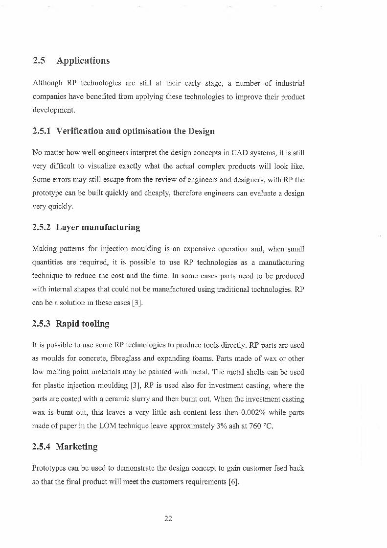
normally approximated by series of triangles (STL format), which results in chordal
error see Figure 16. This chordal error leads to a non-smooth surface. To generate a
STL file model, a tolerable chordal error has to be set. A small tolerance value results
in an increased number o f facets, increasing the file size and part build time.
23
Chordal Error
Figure 16 Chordal error between actual surface and tessellated surface
M ost RP software effort focuses on geometry verification o f the STL CAD model
prior to part fabrication [14, 37]. The need to improve the STL format or its
processing has been recognised. Many approaches have been proposed, one approach
is to use other existing data formats such as IGES, HPGL, STEP and CT data; other
approaches are under investigation such as NURBS and direct slicing methods [1, 34,
2. Process planning errors
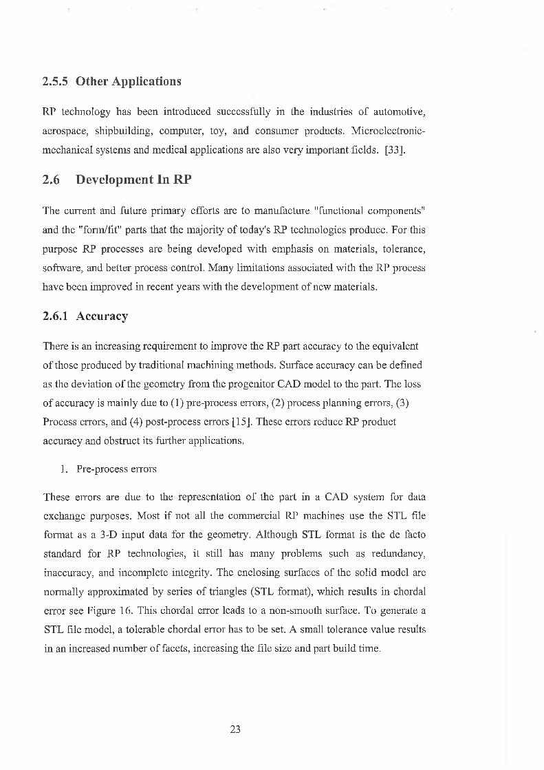
The staircase effect is a result of the slicing process and therefore a common source of
dimensional inaccuracy in RP. The staircase effect can be measured by the layer
thickness and the angle between the vertical and surface tangent.
This error can be quantified by cusp height, which is the distance between the
intended and approximated surface at each facet Figure 17, or may be represented as
the volumetric deviation [36], which can be evaluated by calculating the volumetric
error for each layer to give the overall volumetric deviation.
35],
Figure 17 The stair-step effect due to layer thickness.
24
Some systems reduce the staircase effect by optimising the build direction for each
layer. Layers are then added at various angles using a five axis tool head [37] or
smoothed through staircase machining [38].
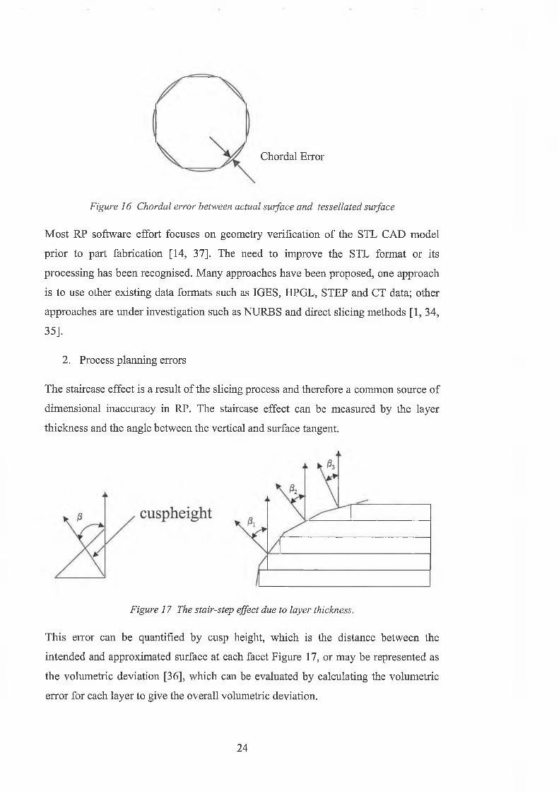
Most RP systems deposit material in only one direction, and reduction of the staircase
effect can be achieved by slicing the part using a smaller layer thickness causing
longer RP fabrication time. An adaptive slicing approach improves the surface quality
and shortens the build time for RP see Figure 18. The variable layer thickness
produces very thin layers, especially when slicing objects having curved surfaces, so
that the build time may therefore still be very long [39], Local adaptive slicing
improves the surface quality and shortens the build time, using this method only the
skin regions have thin layers to ensure a smooth part surface. The internal areas will
be processed with the maximum allowable layer thickness o f a particular process [5,
40],
(a) Normal slicing (b) Adaptive slicing (c) Advanced adaptive slicing
Figure 18 Methods o f slicing to reduce the staircase errors
3. Process errors
Process errors are mainly due to laser delivery mechanisms in SLA and SLS, the
induced angle with the part surface and the beam width. The beam width is not
constant from machine to machine and not constant even on the same machine over
time [34], Other process errors can occur because of the speed of recoating the resin
and the flatness of the resin surface. In FDM the width o f the material delivered and
its temperature can result in errors. In SLS and 3DP, the flatness of the powder spread
and its density and different parameter set-ups will generate different machining
accuracy and build time.
A better laser beam control mechanism and beam width compensation software has
been used, which reduces the error to a minimum in SLA and SLS [34],
25
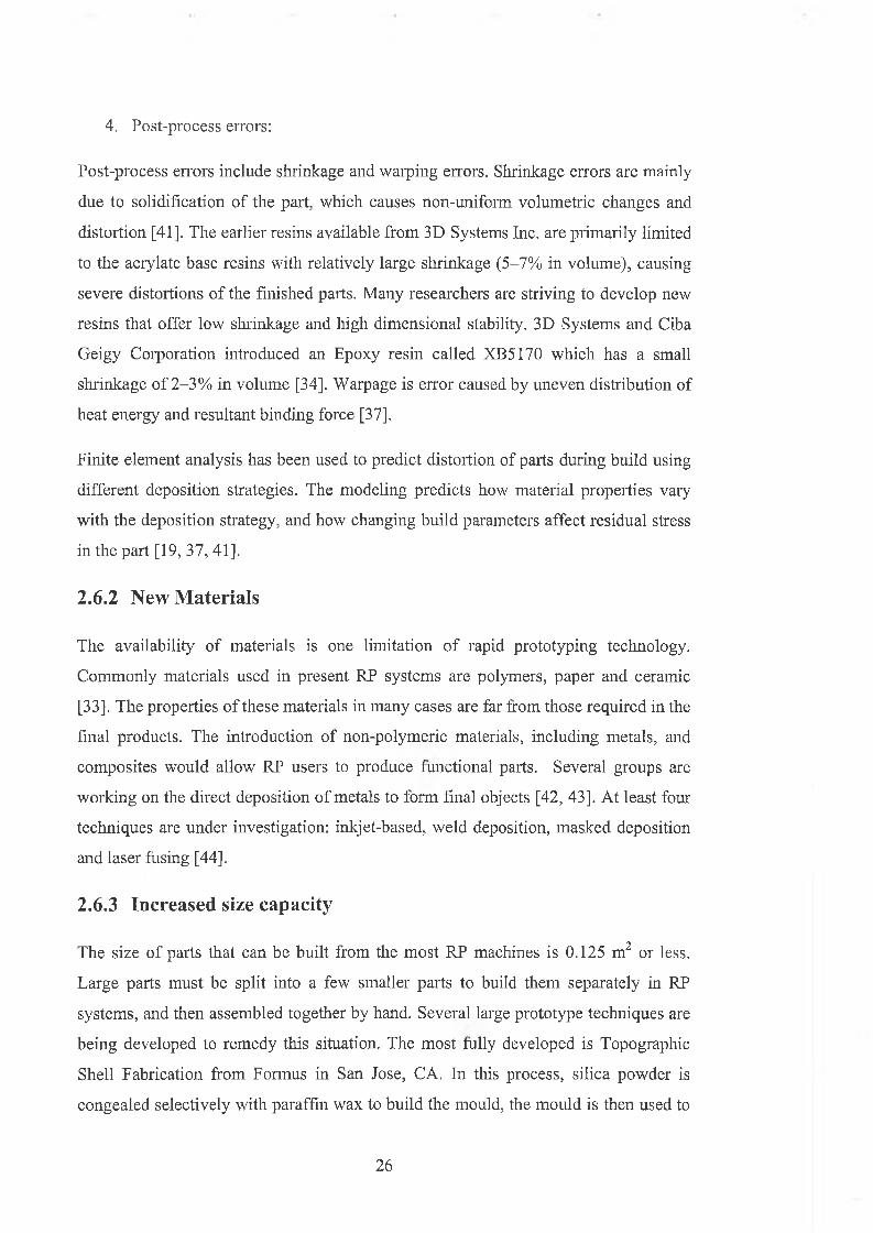
4. Post-process errors:
Post-process errors include shrinkage and waiping errors. Shrinkage errors are m ainly
due to solidification of the part, which causes non-uniform volumetric changes and
distortion [41]. The earlier resins available from 3D Systems Inc. are primarily limited
to the acrylate base resins with relatively large shrinkage (5-7% in volume), causing
severe distortions of the finished parts. Many researchers are striving to develop new
resins that offer low shrinkage and high dimensional stability. 3D Systems and Ciba
Geigy Corporation introduced an Epoxy resin called XB5170 which has a small
shrinkage o f 2-3% in volume [34], Warpage is error caused by uneven distribution of
heat energy and resultant binding force [37].
Finite element analysis has been used to predict distortion of parts during build using
different deposition strategies. The modeling predicts how material properties vary
with the deposition strategy, and how changing build parameters affect residual stress
in the part [19, 37, 41].
2.6.2 New Materials
The availability of materials is one limitation o f rapid prototyping technology.
Commonly materials used in present RP systems are polymers, paper and ceramic
[33]. The properties o f these materials in many cases are far from those required in the
final products. The introduction of non-polymeric materials, including metals, and
composites would allow RP users to produce functional parts. Several groups are
working on the direct deposition of metals to form final objects [42, 43]. At least four
techniques are under investigation: inkjet-based, weld deposition, masked deposition
and laser fusing [44],
2.6.3 Increased size capacity
The size of parts that can be built from the most RP machines is 0.125 m2 or less.
Large parts must be split into a few smaller parts to build them separately in RP
systems, and then assembled together by hand. Several large prototype techniques are
being developed to remedy this situation. The most fully developed is Topographic
Shell Fabrication from Fonnus in San Jose, CA. In this process, silica powder is
congealed selectively with paraffin wax to build the mould, the mould is then used to
2 6
produce fibreglass, epoxy, foam, or concrete models up to 3.3m by 2m by 1.2 m in
size [45].
2.6.4 Build-time
Build-time can be defined as the time required for building a physical part. In SLS
and, SLA the build-time depends on the total recoating time consumed between layers
and the laser scan time used at each layer, and both of them are functions of part size
and geometry [15, 33]. Rapid prototyping machines are still slow by some standards.
By using faster computers, more complex control systems, and improved materials,
RP manufacturers are dramatically reducing building time. 3D System introduced its
SLA7000 machine, which can produce models three times faster than previous SLA
machines [23].
2.6.5 Multiple material objects
Some RP machines have the capability to fabricate multiple material objects (FGM).
To fabricate a multiple material object, a very complicated process is employed, first
the material has to be represented in the CAD design, the material information has to
be transferred to a STL file, the processor has to slice the STL file and find the areas
for each material [46]. Some papers proposed a scheme for representing multiple
material objects in a CAD system. A material tree of the object is built in the CAD
system's data structure. Extracting information from this material tree, and outputting
a modified version of a STL file format to the RP machines could allow fabrication of
multiple material objects [5, 46]
2.6.6 Extension the Applications of Rapid Prototyping
As RP technology has been introduced successfully in many industrial applications, a
new trend has also developed in other areas o f work. Sculptors are beginning to use
RP, as a method of producing complicated structures. Producing jewellery is another
field in which RP technology is being used. Medical application is another very
important field o f application [20]. Now human organ models can be produced by
means of using RP technology and medical digital imaging systems. As the machinery
required becomes cheaper and the range of materials and processes increases RP is
likely to become a method o f manufacturing [22].
27
2.7 Computer Aided Design (CAD)
Computer Aided Design is defined as using the computer to assist in creation and
modification of a design. The operator uses the input device such as a mouse, key
board, digitiser tables, joy stick, or light pen to specify the points and lines on the
display screen. The function menu assists the user in manipulating these simple
entities to build a complex geometry. The graphic system allows the user to move,
rotate, flip, magnify, mirror, copy, and erase entities. The frequently used drawing can
be stored in a library and recalled instead of redrawing them each time [2, 47],
When CAD systems appeared in the late 1960’s they were working only in two
dimensions, their capabilities were improved in early 1970s to include three-
dimensional wire frame and surface modelling. Wire frames contain only information
about part edges and comers, surface models define the outside envelop of part
geometry. By the mid-1980s all major CAD products had solid modelling capabilities,
solid modelling allows the computer to determine the volume that is included within
the object's bounding surface, moments of inertia, centres of gravity, and other mass
properties can be computed.
CAD systems increased design accuracy, consistency between drawings, and
improved the drawing speed. The greatest improvements were experienced in tasks
where drawings are changed frequently or which contain repetitive or standard details
[2, 47]. One of the greatest benefits o f CAD is using the geometric data to perform
other functions in computer aided engineering and in computer aided manufacturing,
this reduces the time and the errors caused by redefining the geometry from scratch in
the other systems.
2.8 Computer Aided Manufacturing (CAM)
Computer Aided Manufacturing is defined as a technique of using a computer and
supporting processing software to actually produce the parts on the factory floor.
Factory equipment can include robots, multiple-axis machine tools, and
programmable controllers. These devices often are grouped in flexible manufacturing
centres to produce different parts.
28
Numerical control (NC) is the most mature area o f CAM, it is a technique of using
programmed instructions to control a machine tool that mills, cuts, punches etc.
Instructions were originally stored on punched paper tapes or magnetic tapes. In
Computer Numerical Control (CNC) a dedicated mini computer stores part process
data and controls the machine. In the distributed numerical control (DNC) systems
instructions come from a centralized computer via net work or direct connection.
Programming of robots is another area o f CAM. Robots perform different tasks such
as welding, assembly, carry equipment and parts around the shop floor or moving
workpieces for NC machines. CAM extend as robot capabilities to more advanced off
line programming, in which robot instructions are provided by a computer, which
automatically determines motion paths and grip points [2].
2.9 Computer Aided Design and Manufacturing CAD/CAM
Writing NC programs manually is a time-consuming and error-prone process
requiring an experienced programmer to write instructions directly from engineering
drawings, run the program on an actual machine tool, and refine it several times until
it works properly. Now the computer itself can generate NC instructions based on
geometric data from the CAD database, plus additional information supplied by the
operator. Many systems have this capability built into their software package. In fact
CAD/CAM software usually refers to a CAD package with an NC programming
feature built in [2]. In some systems the CAD/CAM software tests the program in a
simulated machining process, the software will note and report programming syntax
errors before execution and will supply diagnostics. Once a program is syntactically
correct, the computer will simulate execution of the program and will construct a
drawing of a machined part. When the satisfactory program is achieved, the software
will issue the program to a CNC machine for execution and can store the program on
disk for future production runs [48].
29
2.10 Principle Of Numerical Control
In numerical control machines the control systems read the programme designed to
produce a part, without human operators. The program contains commands to direct
the motion of the cutting tool or movement of the part against a rotating tool or to
change the cutting tools.
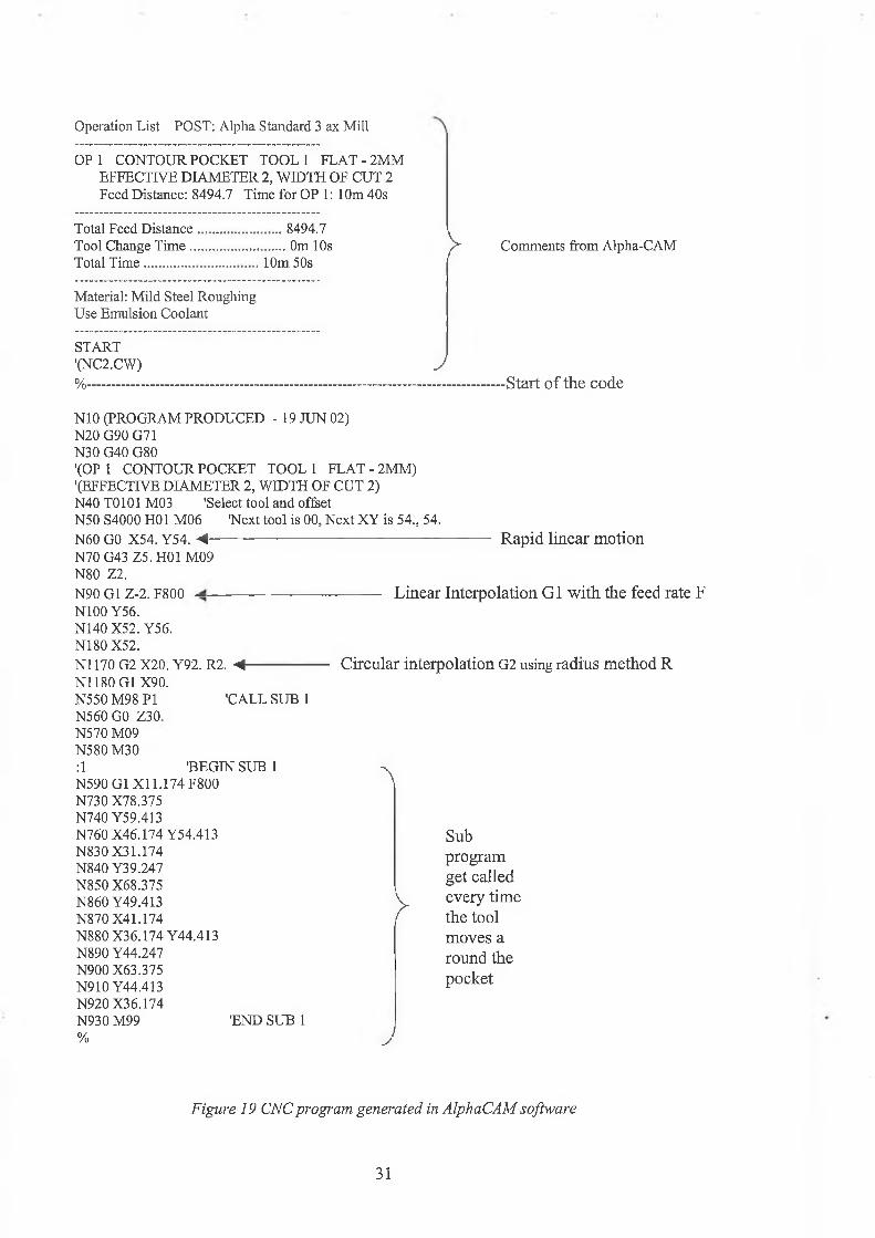
2.10.1 CNC Program Structure
The CNC program contains of one or more blocks, each block contains one or more
words, and the word made up of a letter address (X, Y, Z, R, etc.) followed by a value,
see Figure 19 [49,50].
The machine control executes each block in turn. The words in a block are executed
in a specific order. For example an M code instruction is executed before any axis
movement in the block. [49, 50, 51]
2.10.2 G-Codes
G codes specify the preparatory functions. They prepare the machine for what to do
next. [49] There are two types o f G commands modal and non-modal. Modal
commands come in groups, for example G17, G18 and G19 are one group. Only one
code in a group may be activated at any time. Programming another code in that
group switches to another mode. The non-modal commands affect only the program
block in which they appear, see Appendix A [50, 51]
2.10.3 Absolute and Incremental Mode
There are two methods of entering new positions into a CNC program, One is relative
to the current Datum or Zero Point, called an absolute mode, and controlled with G90.
The other relative to the current tool position called incremental mode and controlled
with G91. G90 and G91 are group modal and will be effective until the next G is
programmed.
30
Operation List POST: Alpha Standard 3 ax Mill
OP1 CONTOUR POCKET TOOL 1 FLAT - 2MM EFFECTIVE DIAMETER 2, WIDTH OF CUT 2 Feed Distance: 8494.7 Time for OP 1: 10m 40s
Total Feed Distance.......... ........... 8494.7Tool Change Time............... .........0m 10sTotal Time................. ............ 10m 50s
Material: Mild Steel Roughing Use Emulsion Coolant
START'(NC2.CW)%........................................................................................................................
> Comments from Alpha-CAM
J-Start o f the code
N10 (PROGRAM PRODUCED - 19 JUN 02)N20 G90 G71 N30 G40 G80'(OP 1 CONTOUR POCKET TOOL 1 FLAT - 2MM) '(EFFECTIVE DIAMETER 2, WIDTH OF CUT 2)N40 T0101 M03 'Select tool and offsetN50 S4000 H01 M06 'Next tool is 00, Next XY is 54., 54.N60 GO X54. Y54. <-------------------------------------------------N70G43 Z5.H01 M09 N80 Z2.N90 G1 Z-2. F800 ---------------------N100 Y56.N140 X52. Y56.N180 X52.N1170 G2 X20. Y92. R2. < ----------- -N1180 G1 X90.
Rapid linear motion
Linear Interpolation G l with the feed rate F
Circular interpolation G2 using radius method R
N550M98P1 N560 GO Z30 N570 M09 N580 M30 :1N590 Gl XI 1.174 F800 N730 X78.375 N740 Y59.413 N760 X46.174 Y54.413 N830X31.174 N840 Y39.247 N850 X68.375 N860 Y49.413 N870 X41.174 N880 X36.174 Y44.413 N890 Y44.247 N900 X63.375 N910 Y44.413 N920 X36.174 N930 M99 %
'CALL SUB 1
'BEGIN SUB 1A
>
'END SUB 1
Subprogram get called every time the tool moves a round the pocket
J
Figure 19 CNCprogram generated in AlphaCAM software
31
2.10.4 Motion Commands
There are only four commonly used commands to determine the motion of CNC
machines GO, G l, G2, and G3. GO is rapid interpolation, G1 is linear interpolation
with the feed rate in F, G2 is circular interpolation in clockwise direction, and G3 is
circular interpolation in counter clockwise direction.
All motion commands are modal commands, meaning they remain in effect until
changed or cancelled [49,51]. Below an explanation of GO, G1,G2 and G3 is
presented.
1. Rapid Linear motion GO:
This command is used to position the CNC machine close to the workpiece. In this
mode the tool will move at the fastest possible rate to the programmed point.
2. Linear Interpolation G l :
In this mode the tool will move along a straight line. The control moves the tool to the
programmed point at feed rate defined by the word F in the same block.
3. G2 and G3 Circular interpolation:
In this mode the tool will move along a circular arc with a specific feed rate, two axes
will always move together in the current plane. For most machines G2 represents
clockwise motion and G3 represent counter-clockwise motion. There are two methods
o f determining the radius of the arc. Either the radius is programmed using the R
command or the centre is described using the I,J and K command.
1. I's. J's and K ’s method: Some older CNC controls do not allow the
programmer to specify circular motion with a radius command. They require
the programmer to specify the location o f the centre point o f the arc. The most
common method of using I, J and K in circular commands involves knowing
the distance and direction from the start point to the centre of the arc
I: is the distance and direction from the starting point of the arc to the
centre of the arc along the X-axis.
32

J is the distance and direction from the starting point o f the arc to the
centre of the arc along the Y-axis.
K is the distance and direction from the starting point o f the arc to the
centre of the arc along the Z-axis. [49]
2. Radius method: The most common and simple way for specifying circular
motion on current controls is by specifying the radius of the arc along with the
end point see Figure 20. The control will automatically figure out how to make
the circular motion.
Figure 20 Illustration o f variables used in circular interpolation
33
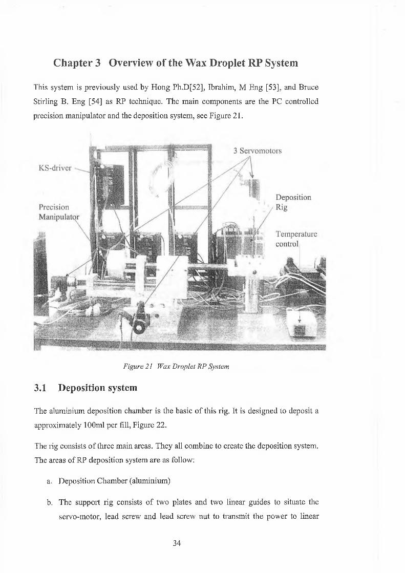
Chapter 3 Overview of the Wax Droplet RP System
This system is previously used by Hong Ph.D[52], Ibrahim, M Eng [53], and Bruce
Stirling B. Eng [54] as RP technique. The main components are the PC controlled
precision manipulator and the deposition system, see Figure 21.
Figure 21 Wax Droplet RP System
3.1 Deposition system
The aluminium deposition chamber is the basic o f this rig. It is designed to deposit a
approximately 100ml per fill, Figure 22.
The rig consists o f three main areas. They all combine to create the deposition system.
The areas of RP deposition system are as follow:
a. Deposition Chamber (aluminium)
b. The support rig consists o f two plates and two linear guides to situate the
servo-motor, lead screw and lead screw nut to transmit the power to linear
34
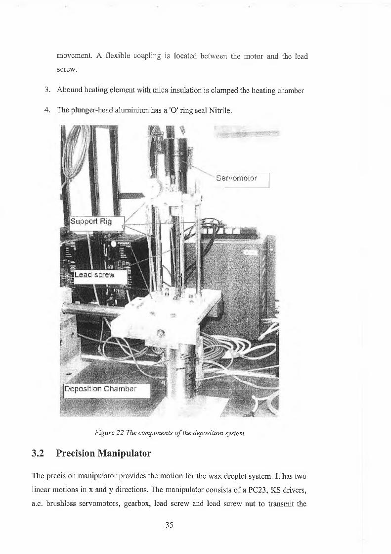
3. Abound heating element with mica insulation is clamped the heating chamber
4. The plunger-head aluminium has a 'O' ring seal Nitrile.
movement. A flexible coupling is located between the motor and the lead
screw.
Figure 22 The components o f the deposition system
3.2 Precision Manipulator
The precision manipulator provides the motion for the wax droplet system. It has two
linear motions in x and y directions. The manipulator consists of a PC23, KS drivers,
a.c. brushless servomotors, gearbox, lead screw and lead screw nut to transmit the
35
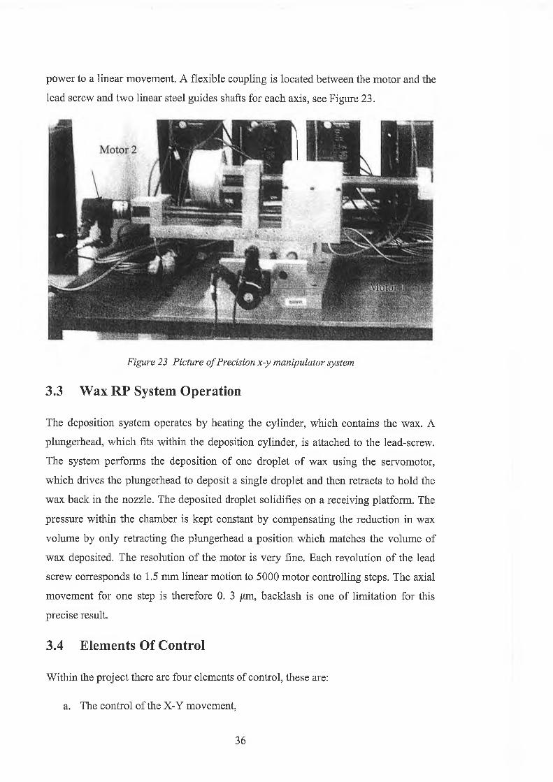
power to a linear movement. A flexible coupling is located between the motor and the
lead screw and two linear steel guides shafts for each axis, see Figure 23.
Figure 23 Picture o f Precision x-y manipulator system
3.3 Wax RP System Operation
The deposition system operates by heating the cylinder, which contains the wax. A
plungerhead, which fits within the deposition cylinder, is attached to the lead-screw.
The system performs the deposition of one droplet o f wax using the servomotor,
which drives the plungerhead to deposit a single droplet and then retracts to hold the
wax back in the nozzle. The deposited droplet solidifies on a receiving platform. The
pressure within the chamber is kept constant by compensating the reduction in wax
volume by only retracting the plungerhead a position which matches the volume of
wax deposited. The resolution o f the motor is very fine. Each revolution o f the lead
screw corresponds to 1.5 mm linear motion to 5000 motor controlling steps. The axial
movement for one step is therefore 0. 3 /xm, backlash is one of limitation for this
precise result.
3.4 Elements Of Control
Within the project there are four elements of control, these are:
a. The control of the X-Y movement,
36
b. The deposition control, and
c. The heating control.
These are each very important and all influence the final output.
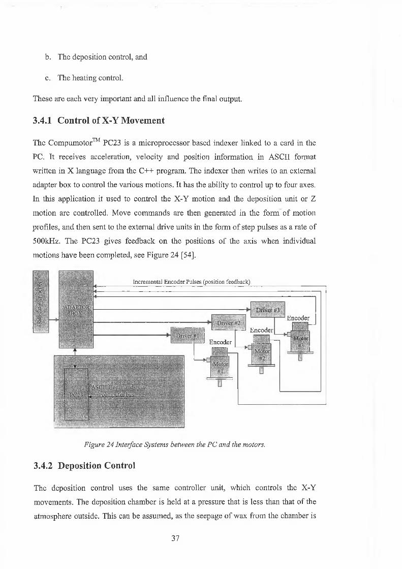
3.4.1 Control of X-Y Movement
The Compumotor™ PC23 is a microprocessor based indexer linked to a card in the
PC. It receives acceleration, velocity and position information in ASCII format
written in X language from the C++ program. The indexer then writes to an external
adapter box to control the various motions. It has the ability to control up to four axes.
In this application it used to control the X-Y motion and the deposition unit or Z
motion are controlled. Move commands are then generated in the form of motion
profiles, and then sent to the external drive units in the form of step pulses as a rate of
500kHz. The PC23 gives feedback on the positions of the axis when individual
motions have been completed, see Figure 24 [54].
Driver '#3
Encoder
Encoder
Encoder
.Motor
Incremental Encoder Pulses (position feedback)
Figure 24 Interface Systems between the PC and the motors.
3.4.2 Deposition Control
The deposition control uses the same controller unit, which controls the X-Y
movements. The deposition chamber is held at a pressure that is less than that of the
atmosphere outside. This can be assumed, as the seepage o f wax from the chamber is
37
much greater when the plungerhead is in situ than when the plunger is out of the
chamber. The basis o f the deposition control is plunging and retracting movement.
This allows a single droplet of wax to form and drop from the nozzle o f the chamber
on the forward plunge generated movement. Then the retraction of the plungerhead
causes the low-pressure within the chamber to suck the excess wax back into the
chamber. Thereby allowing the controlled deposition of wax droplets from the
chamber.
3.5 X language and Position modes
In X language there are three positioning modes that can be used to manipulate the
motor, see Appendix B for more commands. The three modes are normal, alternating,
and continuous.
3.5.1 Normal (Preset) mode
Preset moves can be selected by putting the PC23 into normal mode using the MN
command. Normal mode allows positioning of the motor in incremental moves or
absolute moves.
a. Incremental moves: allows positioning the motor in relation to the motor’s
previous stop position. Incremental movement is selected using the Mode
Position Incremental (MPI or FAS 0 ) command. This is the default (Power-
up) positioning mode.
1. Absolute moves: allows positioning the motor in relation to a defined zero
reference position. Absolute move can be selected using the Mode Position
Absolute (MPA or FASA1) command. The current position is set to be
absolute zero reference point by issuing the Position Zero (PZ) command, or
by cycling the power to the indexer. Issuing the Go Home (GH) command
moves the axes to their absolute zero position. The PC23 retains the absolute
position, even while the unit is in the incremental mode.
3.5.2 Alternating Mode
In this mode after issuing the Go (G) command, the motor shaft rotates to the
commanded position, which corresponds to the value set by the “D ” command. And
38

then retraces its path back to the start position. The shaft continues to move between
the start position and the command position. The motor stops immediately when the
“S” command is issued. However if SSD1 command is issued before the G command,
then when S command is issued the motor completes the cycle and stops at the start
position see Appendix B.
3.5.3 Continuous Mode
In this mode when a G command is issued the motor continues to rotate in a constant
movement for a period of time rather than a fixed distance. It can be synchronized to
external events such as trigger input signals. Velocity and acceleration can be changed
while the motor is in continuous motion, by issuing a new V and A command
followed by a G command.
39
Chapter 4 Development Of The System
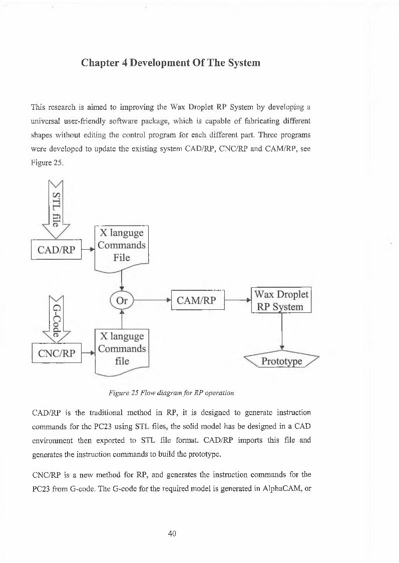
This research is aimed to improving the Wax Droplet RP System by developing a
universal user-friendly software package, which is capable of fabricating different
shapes without editing the control program for each different part. Three programs
were developed to update the existing system CAD/RP, CNC/RP and CAM/RP, see
Figure 25.
Figure 25 Flow diagram for RP operation
CAD/RP is the traditional method in RP, it is designed to generate instruction
commands for the PC23 using STL files, the solid model has be designed in a CAD
environment then exported to STL file format. CAD/RP imports this file and
generates the instruction commands to build the prototype.
CNC/RP is a new method for RP, and generates the instruction commands for the
PC23 from G-code. The G-code for the required model is generated in AlphaCAM, or
40
any CAM software, and then saved as a text file, CNC/RP imports this file and
generates instruction commands to build the prototype.
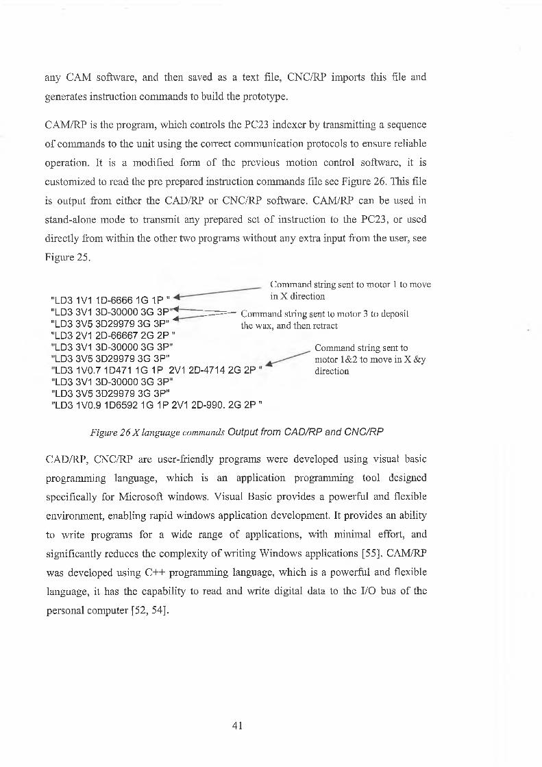
CAM/RP is the program, which controls the PC23 indexer by transmitting a sequence
o f commands to the unit using the correct communication protocols to ensure reliable
operation. It is a modified form of the previous motion control software, it is
customized to read the pre prepared instruction commands file see Figure 26. This file
is output from either the CAD/RP or CNC/RP software. CAM/RP can be used in
stand-alone mode to transmit any prepared set of instruction to the PC23, or used
directly from within the other two programs without any extra input from the user, see
Figure 25.
"LD3 1V1 1D-6666 1G 1P " m A uireouon"LD3 3V1 3D-30000 3G 3P"^ — -— Command string sent to motor 3 to deposit"LD3 3V5 3D29979 3G 3P" the wax, and then retract"LD3 2V1 2D-66667 2G 2P "
"LD3 3V1 3D-30000 3G 3P""LD3 3V5 3D29979 3G 3P""LD3 1V0.9 1D6592 1G 1P 2V1 2D-990. 2G 2P "
Figure 26Xlanguage commands Output from CAD/RP and CNC/RP
CAD/RP, CNC/RP are user-friendly programs were developed using visual basic
programming language, which is an application programming tool designed
specifically for Microsoft windows. Visual Basic provides a powerful and flexible
environment, enabling rapid windows application development. It provides an ability
to write programs for a wide range of applications, with minimal effort, and
significantly reduces the complexity o f writing Windows applications [55]. CAM/RP
was developed using C++ programming language, which is a powerful and flexible
language, it has the capability to read and write digital data to the I/O bus of the
personal computer [52, 54].
Command string sent to motor 1 to move in X direction
LD3 3V1 3D-30000 3G 3P"LD3 3V5 3D29979 3G 3P"LD3 1V0.7 1D471 1G 1P 2V1 2D-4714 2G 2P
Command string sent to motor 1&2 to move in X &y direction
41
4.1 Development of CAM/RP software
The main task for this software is to communicate with the PC23. To operate the
PC23 with X language commands, the software has to have the capabilities of reading
information from and writing data to I/O bus of the personal computer.
Communication with the PC23 involves two pairs o f registries. A register refers to a
temporary storage area for holding one character. Data transfer to and from the
register takes place one character at time.
The motion control commands and responses are transferred through the input data
buffer (IDB) and output data buffer (ODB) at the indexer’s based address 300Hex.
Interface control commands and status information are transferred through the control
byte (CB) and status byte (SB) at one address location above the base address, 301
Hex.
The ODB and SB are read-only registers. The IDB and the CB are write only register.
Compumotor™ provides a sample read and write routines that access the computer’s
I/O bus.
X language commands are strings o f ASCII characters. Passing a command to the
indexer requires transferring each character in the command one a time. Each
character transfer requires that the sender notify the receiver that a character is ready,
and that the receiver notifies the sender that the character has been received. The
notification process involves setting or clearing control bits (flags) SB and CB
registers.
Control Byte CB flags allow the program to signal the PC23 with messages. The
status Byte flags allow the host program to report the operation conditions such as if
axis # 2 is moving or not.
The PC23 indexer is designed to operate motor axes in a fashion largely independent
of the computer, requiring only a small number o f high level commands and
interaction. The interaction is almost in the form of characters and strings. This
requires knowledge of string handling in the programming language. The program
must include subroutines or procedures to do the following:
42
1. Reset the indexer
2. Send a command string to the indexer.
3. Receive a character string from the indexer.
Hence the PC’s higher execution speed cannot be slowed down using the control
program, the routines for sending commands to the indexer and receiving responses
from the indexer must be changed to solve this problem. The initial routines had a
particular number of loops for communicating with the indexer. The revised routines
will continue to wait until the indexer gives a response.
In previous research the PC23 instruction commands were calculated manually and
hard coded within this program [56]. This means the operator has to find the
deposition positions for each droplet manually, then construct the move command for
each droplet, and then insert these instructions into the motion control program. The
program has to be compiled each time these instructions are changed.
CAM/RP is a modification for the motion control software, which is customized to
read the pre prepared instruction command file line by line, it sends each instruction
to the PC23, and the movement is confirmed by feedback on the positions o f the axes
when each motion has been completed before the next line is read.
The advantage of using CAM/RP that it dose not need to be compiled for each
prototype, also it can be run from CAD/RP or CNC/RP which makes these systems
work in a user-friendly fashion.
43
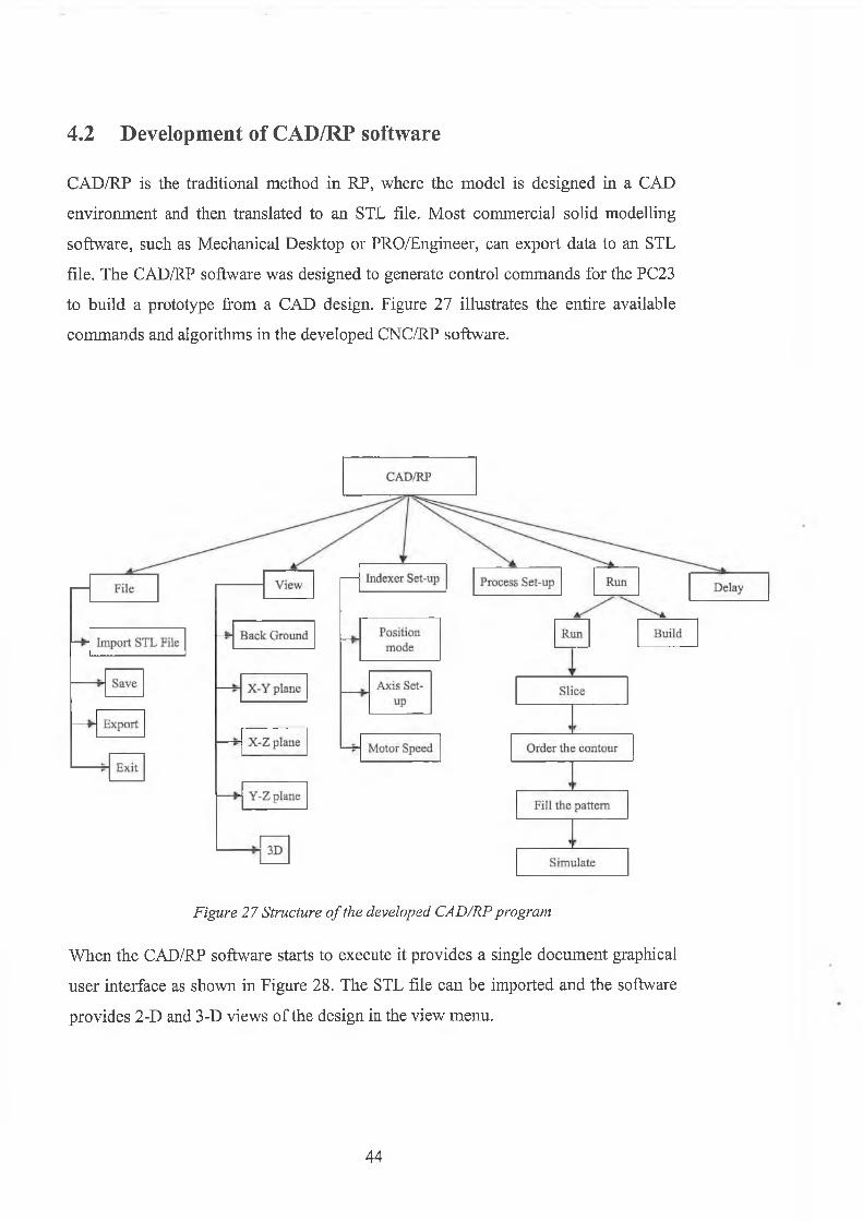
CAD/RP is the traditional method in RP, where the model is designed in a CAD
environment and then translated to an STL file. M ost commercial solid modelling
software, such as Mechanical Desktop or PRO/Engineer, can export data to an STL
file. The CAD/RP software was designed to generate control commands for the PC23
to build a prototype from a CAD design. Figure 27 illustrates the entire available
commands and algorithms in the developed CNC/RP software.
4.2 Development of CAD/RP software
Figure 27 Structure o f the developed CAD/RP program
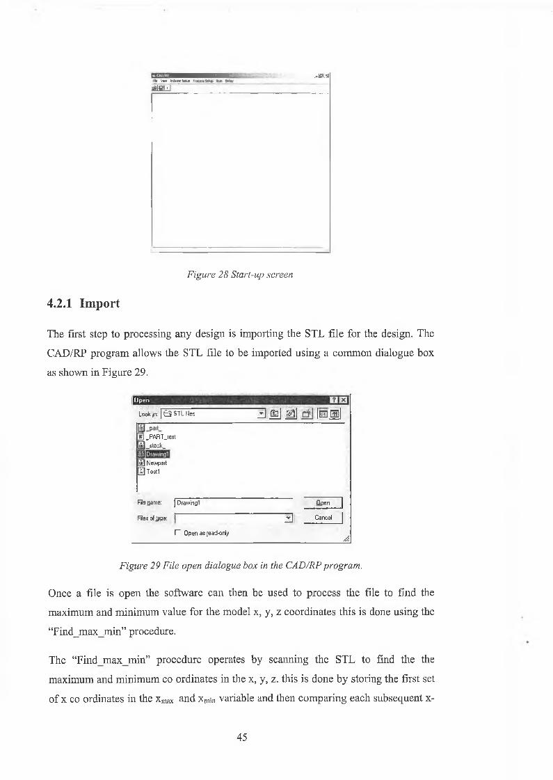
When the CAD/RP software starts to execute it provides a single document graphical
user interface as shown in Figure 28. The STL file can be imported and the software
provides 2-D and 3-D views of the design in the view menu.
44
Vww ¡«ferwiaÌM» liShIjJ ~
JBJS
Figure 28 Start-up screen
4.2.1 Import
The first step to processing any design is importing the STL file for the design. The
CAD/RP program allows the STL file to be imported using a common dialogue box
as shown in Figure 29.
¡Open
LottKjn: | 0 STL files d Ml Ml Ib ü I
gj .PA R T jex l"£)_:StOCk_
j i j Newpart 3 Test!
Fila flame: j Drawing”
Filet of IvpK
Open
“3 Cancel
I- Open as jead-onlyA
Figure 29 File open dialogue box in the CAD/RP program.
Once a file is open the software can then be used to process the file to find the
maximum and minimum value for the model x, y, z coordinates this is done using the
“Find_max_min” procedure.
The “F in d m a x m in ” procedure operates by scanning the STL to find the the
maximum and minimum co ordinates in the x, y, z. this is done by storing the first set
of x co ordinates in the xmax and xmin variable and then comparing each subsequent x-
45

coordinate with xmax and xmin, overwriting this value with the new coordinate if
necessary. The same time is done for the y and z coordinates
4.2.2 View menu
After importing the design CAD/RP provides the capability to view the design in 2D
and 3D. This gives the ability to ensure that the right design is imported before
starting the slicing process. The view menu contains six commands to view the model,
see Figure 30.
CAD/RP ••• ■■ . ( □ f x j l
File View Indexer Setup Process Setup Run Delay
JÉÌ! Background
X-Y
X-Z
V .7l ~ L
3D
Zoom All
Figure 30 View menu o f CAD/RP program
a. Background colour allows the background colour to be changed. When this
choice is selected a colour dialogue box is called and a desired colour can be
chosen.
a. The X-Y option shows the model in X-Y coordinate system. This selection
calls the function “Cls” to clear the screen, opens the “triangles.txt" file for
input and reads the value for the three vertex and saves only x, y as segments
in a file called “Drawing.txt”, see Appendix C l. After saving these segments
in the “Drawing.txt” text file, The “mnuzoom” procedure called to draw the
view.
b. The X-Z option shows the model in X-Z coordinate system. The same steps
are taken in this procedure but only x and z values are saved as segments.
c. The Y-Z option shows the model in Y-Z coordinate system. The same steps
are taken in this procedure but only y and z values are saved as segments.
46
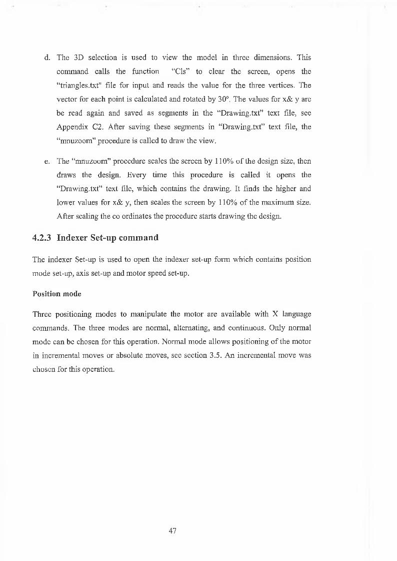
d. The 3D selection is used to view the model in three dimensions. This
command calls the function “Cls” to clear the screen, opens the
“triangles.txt" file for input and reads the value for the three vertices. The
vector for each point is calculated and rotated by 30°. The values for x& y are
be read again and saved as segments in the “Drawing.txt” text file, see
Appendix C2. After saving these segments in “Drawing.txt” text file, the
“mnuzoom” procedure is called to draw the view.
e. The “mnuzoom” procedure scales the screen by 110% o f the design size, then
draws the design. Every time this procedure is called it opens the
“Drawing.txt” text file, which contains the drawing. It finds the higher and
lower values for x& y, then scales the screen by 110% of the maximum size.
After scaling the co ordinates the procedure starts drawing the design.
4.2.3 Indexer Set-up command
The indexer Set-up is used to open the indexer set-up form which contains position
mode set-up, axis set-up and motor speed set-up.
Position mode
Three positioning modes to manipulate the motor are available with X language
commands. The three modes are normal, alternating, and continuous. Only normal
mode can be chosen for this operation. Normal mode allows positioning o f the motor
in incremental moves or absolute moves, see section 3.5. An incremental move was
chosen for this operation.
47
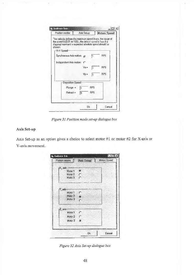
Si. Indexer frm ____________ m -Position m o d e s ]f A xis S e tu p Y P b t o f O B e e d i
T h e velocity defin es th e maximum s p e e d in rps, th e ra n g e of th e s p e e d is (0.01 to 1 S O ), (he defau lt s p e e d is 1 ips.lf a d iagonal m ovm ent is e x p e c te d a b so lu te s p e e d sh o u ld b e ch o sen ,
r X - Y S p a e d — — --------------------------------------
S y n ch ro n o u s Axis m otion {? . H R P S
In d e p e n d e n t Axis m otion C
Vx =
Vy =
h
ITR P S
R P S
O k C an ce l
Axis Set-up
Figure 31 Position mode set-up dialogue box
Axis Set-up as an option gives a choice to select motor #1 or motor #2 for X-axis or
Y-axis .movement.
âi. Indexer lim
Position m odes J f [À xis S e tu p j | M otois S p e e d
I- - x
rX _ ax is -
M otor 1 *
M otoi 2 rM otoi 3 r
rY a x is -
M otor 1 CM otoi 2 (g
M otor 3
-2_ax is-Motor 1 CM otor 2 r
M otor 3 &
O k C ancel
Figure 32 Axis Set-up dialogue box
48

Motor Speed
An absolute motion or the speed for each axis can be chosen for the indexer, If the
absolute value is entered, the speed in the x and y direction will be calculated in the
program. The default motor speed is 1RPS. Deposition speed can also be varied.
i*„ Indexer frm
Position modes [ AwsSelup j i ¡Motor« Speed!
T he velocity delines the maximum speed in tps, th e iange of the speed is [0.01 to ISO), the default speed is lips.lf a diagonal movment is expected absolute speed should b e chosen.
rX-Y S p e e d -
Absolute
Axis rVx =
Vy «
RPS
RPS
RPS
Ok Cancel
Figure 33 Motor speed set-up dialogue box
4.2.4 Process Set-up
After importing and viewing the design the second step is to process this data. Some
important parameters have to be selected before starting the data processing.
The user enters the values for the layer thickness, the filling space which normally
equal to the droplet width, the deposition diameter and the distance between the
droplets, see Figure 34.
49
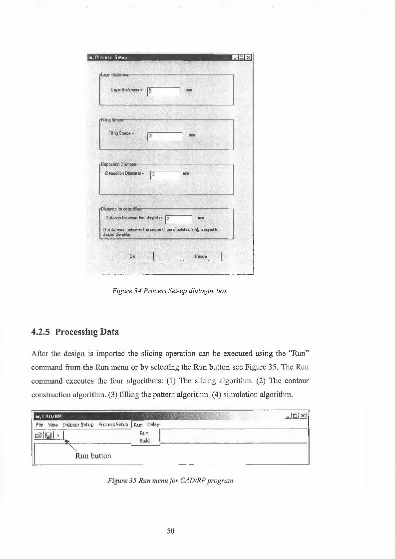
b x s b x h h h h h m h h i i ■ e ë e. ” . . .
l a y e ithickness— —----- ----------------------------------------------- ---------- — —
Layer thickness ■ [H mm
•Filling Space---------
Filing S pace =
Deposition Diameter-— ---------------------------------- -
Deposition Diameter • R mm
■Distance lot deposition------------------------------------------------------------
Distance between the droplets- p mm
The distance between the centei of the droplets usua|y is equal to droplet diameter
Ok_________I Cancel
Figure 34 Process Set-up dialogue box
4.2.5 Processing Data
After the design is imported the slicing operation can be executed using the “Run”
command from the Run menu or by selecting the Run button see Figure 35. The Rim
command executes the four algorithms: (1) The slicing algorithm. (2) The contour
construction algorithm. (3) filling the pattern algorithm. (4) simulation algorithm.
I ÜÚ CAD/RP ■. ' r. 'S ifI'waV _ |□ ! x|
File View In d e x e r S e tu p P ro c e s s S e tu p R u n Delay
E hIh MR un
w Build
\Run button
Figure 35 Run menu for CAD/RP program
50
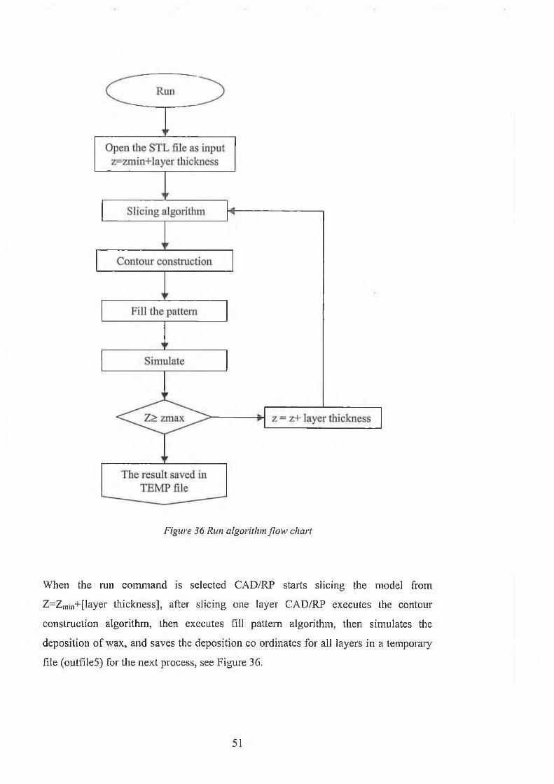
Figure 36 Run algorithm flow chart
When the run command is selected CAD/RP starts slicing the model from
Z=Z,mn+[layer thickness], after slicing one layer CAD/RP executes the contour
construction algorithm, then executes fill pattern algorithm, then simulates the
deposition of wax, and saves the deposition co ordinates for all layers in a temporary
file (outfile5) for the next process, see Figure 36.
51
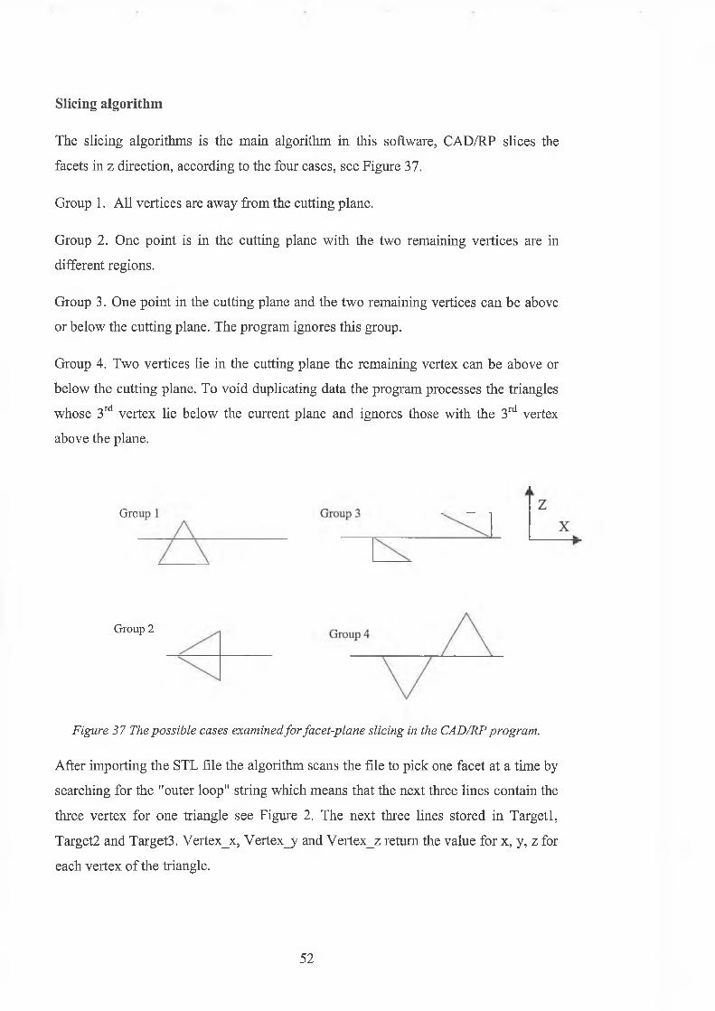
Slicing algorithm
The slicing algorithms is the main algorithm in this software, CAD/RP slices the
facets in z direction, according to the four cases, see Figure 37,
Group 1. All vertices are away from the cutting plane.
Group 2. One point is in the cutting plane with the two remaining vertices are in
different regions.
Group 3. One point in the cutting plane and the two remaining vertices can be above
or below the cutting plane. The program ignores this group.
Group 4. Two vertices lie in the cutting plane the remaining vertex can be above or
below the cutting plane. To void duplicating data the program processes the triangles
whose 3rd vertex lie below the current plane and ignores those with the 3rd vertex
above the plane.
Figure 3 7 The possible cases examined for facet-plane slicing in the CAD/RP program.
After importing the STL file the algorithm scans the file to pick one facet at a time by
three vertex for one triangle see Figure 2. The next three lines stored in Targetl,
Target2 and Target3. Vertex_x, Vertex_y and Vertex_z return the value for x, y, z for
each vertex of the triangle.
Gro
Group 2
searching for the "outer loop" string which means that the next three lines contain the
52
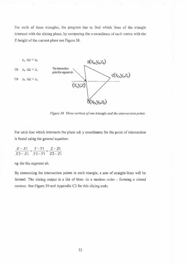
For each of these triangles, the program has to find which lines o f the triangle
intersect with the slicing plane, by comparing the z-coordinate o f each vertex with the
Z-height o f the current plane see Figure 38.
Za <Z < Zb
Or Za <z < zc
Or zi> <z < zc
Figure 38 Three vertices o f one triangle and the entersection poin ts
For each line which intersects the plane x& y coordinates for the point o f intersection
is found using the general equation:
X - X l _ Y - Y l _ Z - Z 1 X 2 - X I ~ Y 2 - Y 1 ~ Z 2 - Z 1
eg: for the segment ab.
By connecting the intersection points in each triangle, a sets of straight-1 ines will be
formed. The slicing output is a list of lines -in a random order - forming a closed
contour. See Figure 39 and Appendix C3 for this slicing code.
53
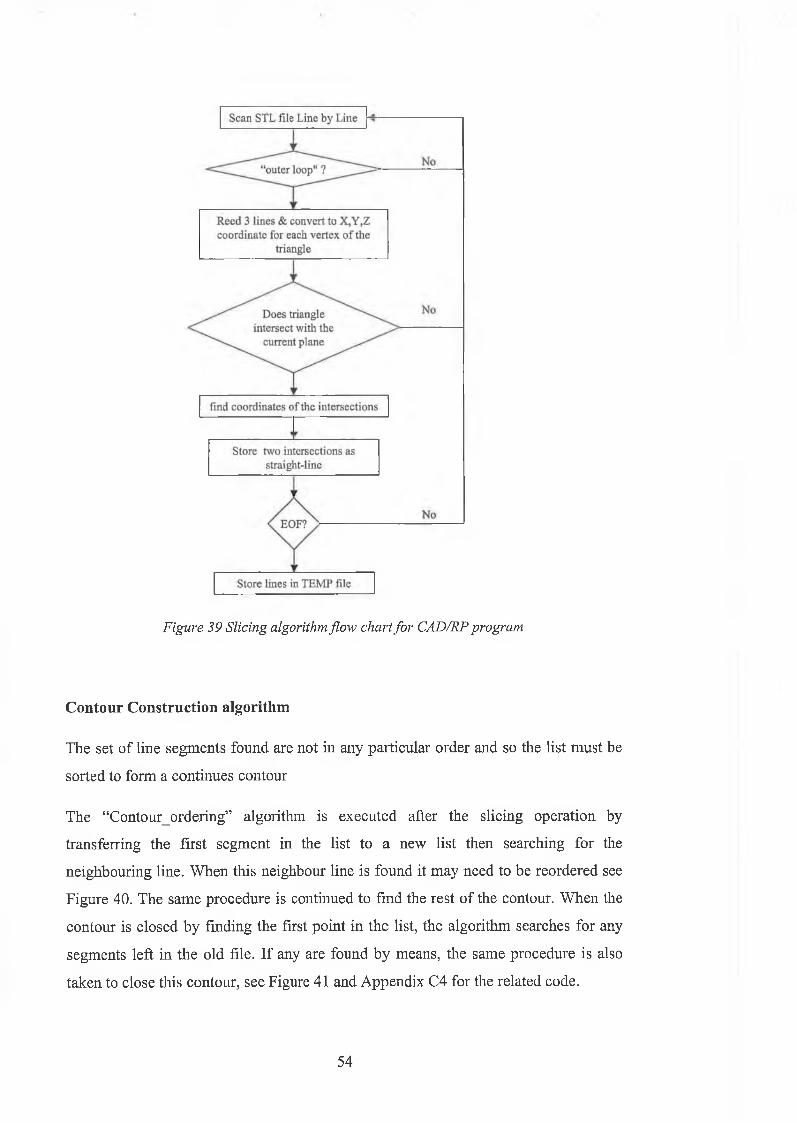
Figure 39 Slicing algorithm flow chart for CAD/RP program
Contour Construction algorithm
The set of line segments found are not in any particular order and so the list must be
sorted to form a continues contour
The “Contour_ordering” algorithm is executed after the slicing operation by
transferring the first segment in the list to a new list then searching for the
neighbouring line. When this neighbour line is found it may need to be reordered see
Figure 40. The same procedure is continued to find the rest of the contour. When the
contour is closed by finding the first point in the list, the algorithm searches for any
segments left in the old file. If any are found by means, the same procedure is also
taken to close this contour, see Figure 41 and Appendix C4 for the related code.
54

bl al
Slicing list
1. (xal,yal),(xbl,ybl)
3. (xa3,ya3),(xb3,yb3)
5. (xa5,ya5),(xb5,yb5)
2. (xb2,yb2),(xa2,ya2)
6. (xb6,yb6),(xa6,ya6)
4. (xb4,yb4),(xa4,ya4)
Intermediate list
l.(xal,yal),(xbl,ybl)
2. (xb2,yb2),(xa2,ya2)L
3. (xa3,ya3),(xb3,yb3)
I4. (xb4,yb4),(xa4,ya4)
5. (xa5,ya5),(xb5,yb5)
6. (xb6,yb6),(xa6,ya6)
Contour list
1. (xal,yal),(xbl,ybl)
2. (xa2,ya2),(xb2,yb2) » t3. (xa3,ya3),(xb3,yb3)
4. {xa4,ya4)>(xb4syb4)
5. (xa5,ya5),(xb5,yb5)
6. (xa6,ya6),(xb6,^b6)
Figure 40 Contour sorting
Figure 41 Contour construction algorithm flow chart fo r CAD/RP program.
55
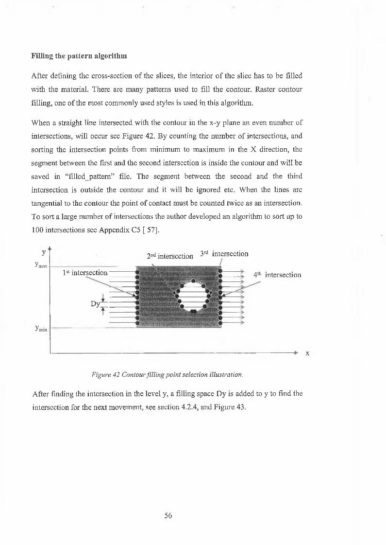
Filling the pattern algorithm
After defining the cross-section of the slices, the interior o f the slice has to be filled
with the material. There are many patterns used to fill the contour. Raster contour
filling, one o f the most commonly used styles is used in this algorithm.
When a straight line intersected with the contour in the x-y plane an even number of
intersections, will occur see Figure 42. By counting the number of intersections, and
sorting the intersection points from minimum to maximum in the X direction, the
segment between the first and the second intersection is inside the contour and will be
saved in “filled_pattem” file. The segment between the second and the third
intersection is outside the contour and it will be ignored etc. When the lines are
tangential to the contour the point of contact must be counted twice as an intersection.
To sort a large number of intersections the author developed an algorithm to sort up to
100 intersections see Appendix C5 [ 57].
y
ymax1st intersection'
Dy:
2nd intersection 3rd intersection\ i¡i;. •' i ]“l
'.v . ■ ‘j ::r -m m -
■i " \S.
V2 i?S£r;- / s.
4th intersection
Figure 42 Contour filling point selection illustration.
After finding the intersection in the level y, a filling space Dy is added to y to find the
intersection for the next movement, see section 4.2.4, and Figure 43.
56
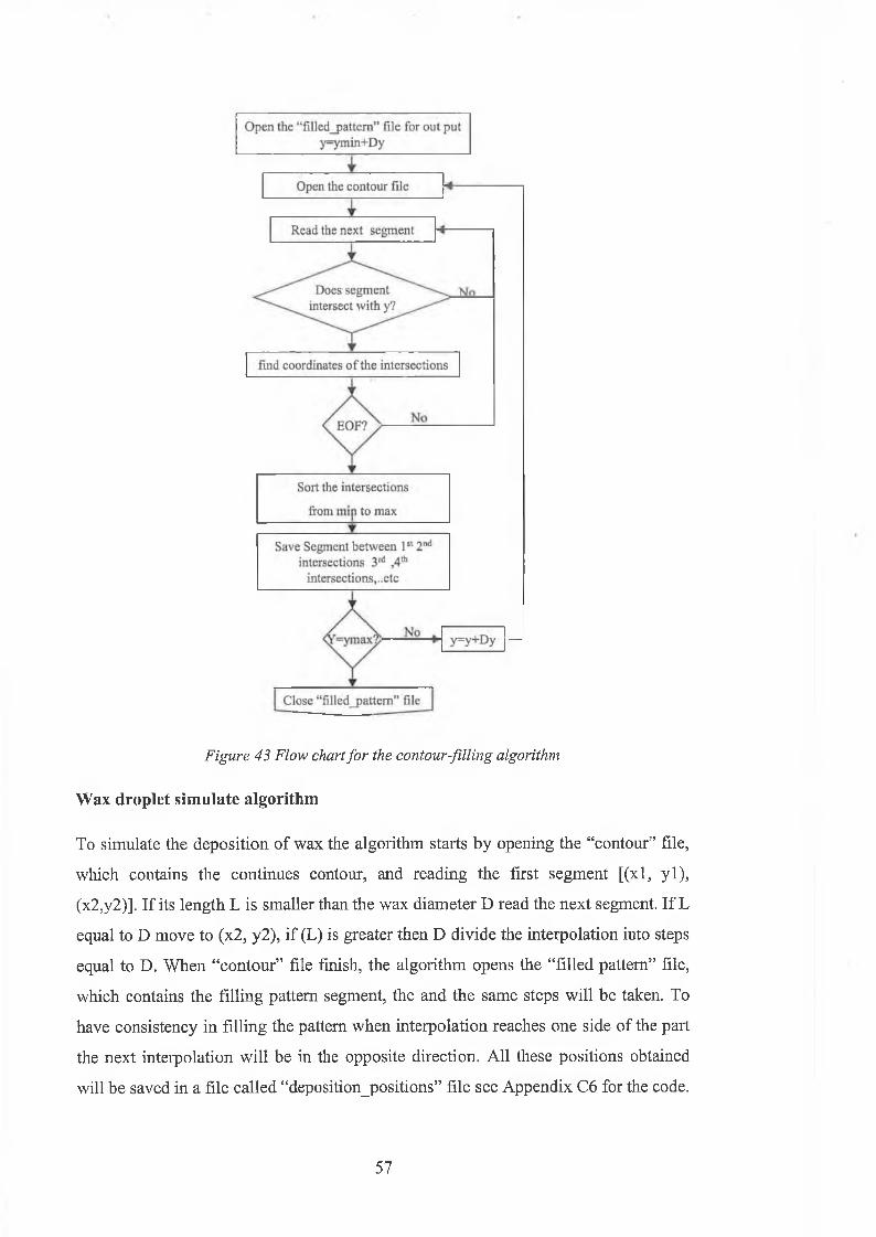
Figure 43 Flow chart for the contour-filling algorithm
Wax droplet simulate algorithm
To simulate the deposition of wax the algorithm starts by opening the “contour” file,
which contains the continues contour, and reading the first segment [(xl, y l),
(x2,y2)]. If its length L is smaller than the wax diameter D read the next segment. If L
equal to D move to (x2, y2), if (L) is greater then D divide the interpolation into steps
equal to D. When “contour” file finish, the algorithm opens the “filled pattern” file,
which contains the filling pattern segment, the and the same steps will be taken. To
have consistency in filling the pattern when interpolation reaches one side of the part
the next interpolation will be in the opposite direction. All these positions obtained
will be saved in a file called “deposition_positions” file see Appendix C6 for the code.
57
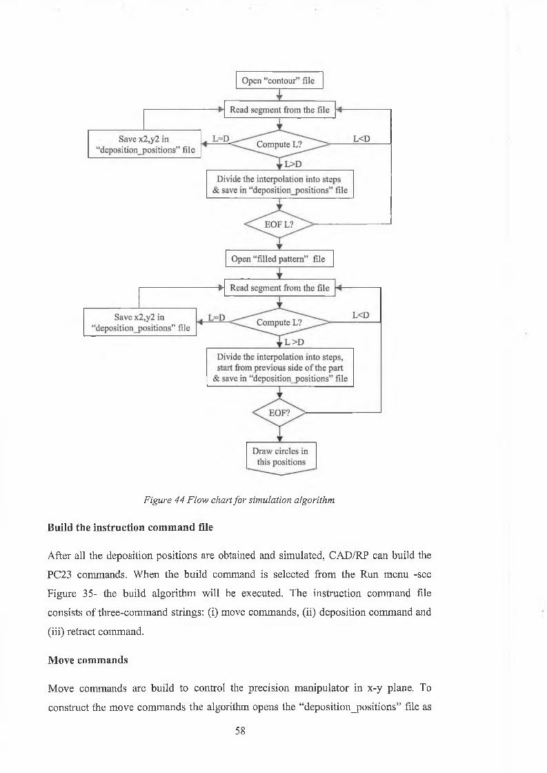
Figure 44 Flow chart for simulation algorithm
Build the instruction command file
After all the deposition positions are obtained and simulated, CAD/RP can build the
PC23 commands. When the build command is selected from the Run menu -see
Figure 35- the build algorithm will be executed. The instruction command file
consists of three-command strings: (i) move commands, (ii) deposition command and
(iii) retract command.
Move commands
Move commands are build to control the precision manipulator in x-y plane. To
construct the move commands the algorithm opens the “deposition_positions” file as
58
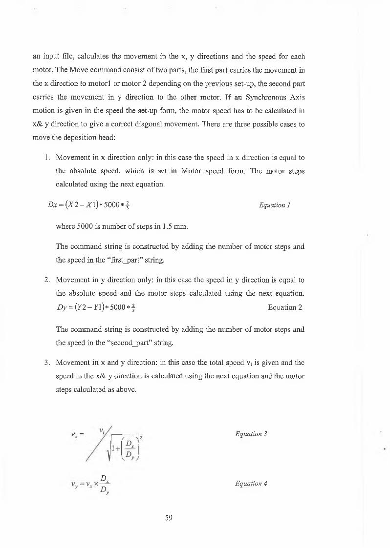
an input file, calculates the movement in the x, y directions and the speed for each
motor. The Move command consist o f two parts, the first part carries the movement in
the x direction to m otorl or motor 2 depending on the previous set-up, the second part
carries the movement in y direction to the other motor. If an Synchronous Axis
motion is given in the speed the set-up form, the motor speed has to be calculated in
x& y direction to give a correct diagonal movement. There are three possible cases to
move the deposition head:
1. Movement in x direction only: in this case the speed in x direction is equal to
the absolute speed, which is set in Motor speed form. The motor steps
calculated using the next equation.
Dx = (X 2 — X \)* 5000 * f Equation 1
where 5000 is number of steps in 1.5 mm.
The command string is constructed by adding the number of motor steps and
the speed in the “first_part” string.
2. Movement in y direction only: in this case the speed in y direction is equal to
the absolute speed and the motor steps calculated using the next equation.
D y = (72 - 71) * 5000 * j Equation 2
The command string is constructed by adding the number of motor steps and
the speed in the “second_part” string.
3. Movement in x and y direction: in this case the total speed vt is given and the
speed in the x& y direction is calculated using the next equation and the motor
steps calculated as above.
v , =
D x
Equation 3
Equation 4
59
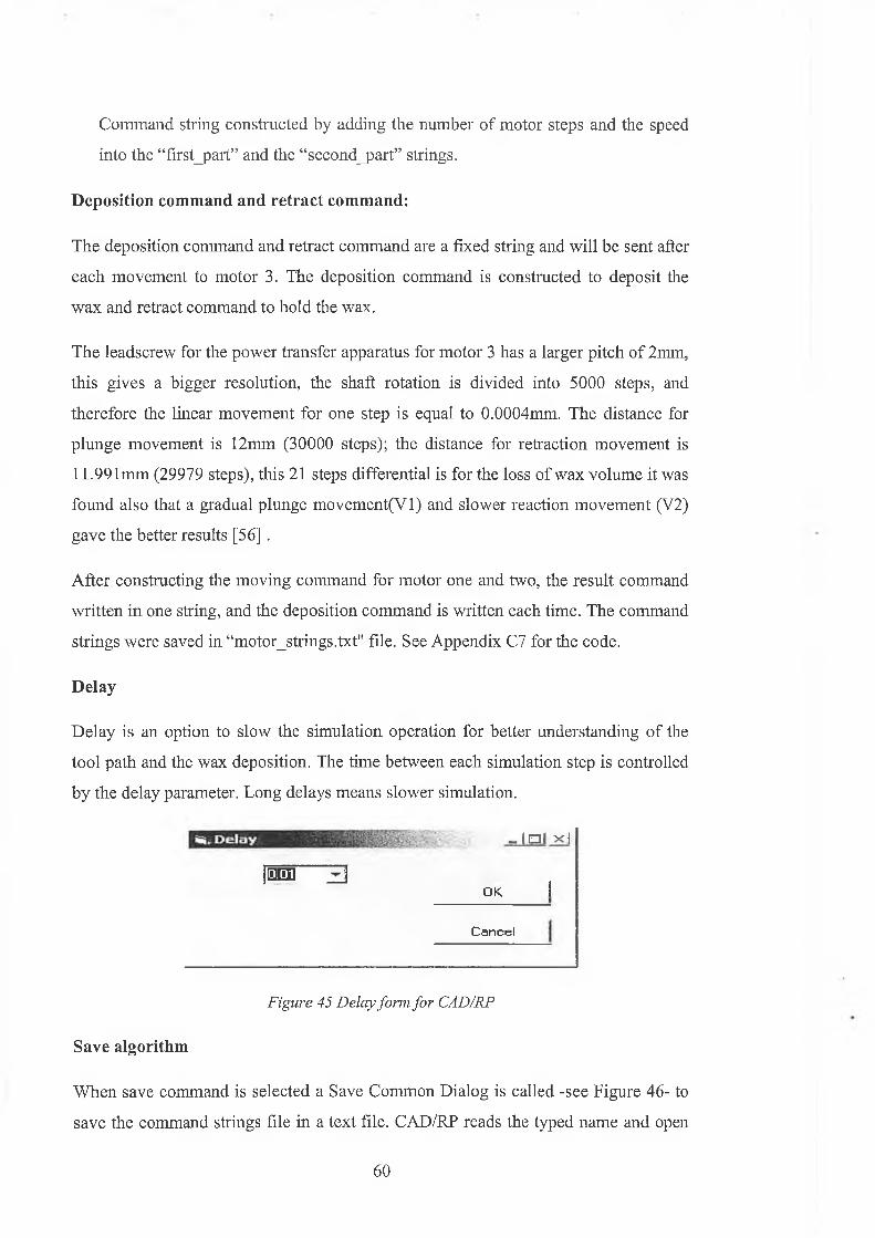
Command string constructed by adding the number of motor steps and the speed
into the “first_part” and the “second_part” strings.
Deposition command and retract command:
The deposition command and retract command are a fixed string and will be sent after
each movement to motor 3. The deposition command is constructed to deposit the
wax and retract command to hold the wax.
The leadscrew for the power transfer apparatus for motor 3 has a larger pitch of 2mm,
this gives a bigger resolution, the shaft rotation is divided into 5000 steps, and
therefore the linear movement for one step is equal to 0.0004mm. The distance for
plunge movement is 12mm (30000 steps); the distance for retraction movement is
11.991mm (29979 steps), this 21 steps differential is for the loss of wax volume it was
found also that a gradual plunge movement(Vl) and slower reaction movement (V2)
gave the better results [56] .
After constructing the moving command for motor one and two, the result command
written in one string, and the deposition command is written each time. The command
strings were saved in “motor_strings.txt" file. See Appendix C7 for the code.
Delay
Delay is an option to slow the simulation operation for better understanding of the
tool path and the wax deposition. The time between each simulation step is controlled
by the delay parameter. Long delays means slower simulation.
l a p 3
Figure 45 Delay form for CAD/RP
Save algorithm
W hen save command is selected a Save Common Dialog is called -see Figure 46- to
save the command strings file in a text file. CAD/RP reads the typed name and open
-Ini xi
O K 1
C a n c e l
60

“motor_strings.txt" for input and the new file name as out put the algorithm reads
from input file and write in the out put file.
File nam e;
S a v e a s type: 13r O p en a s read-only
S a v e A s Q E 3
S a v e jn: | My D o cu m e n ts m mmZD C++ n My eB oo
Z jC N C Iile s Q my mine
2 ] D a ta b a s e D My Musk
Z D D a w à C ] My P ictu
__ 1 L a t te e C D My Videe
1 m icrop tocesso ts C j M y W e b :
! < l 1 ± 1
S a v e
C a n c e l
A
Figure 46 Save common dialogue box
61
4.3 Introduction of Using CAD/CAM for RP
Many existing CAD/CAM software packages are used to generate the tool path for
milling operations. There is a big similarity between the milling operation and
deposition operation. The idea was to use existing CAD/CAM software to generate
the tool path. AlphaCAM™ generates the tool path for CNC machining in G code
format. To use this code for the PC23, software was developed called CNC/RP to
process the G code by performing the next steps:
1. Scanning the CNC code,
2. Manipulating the tool path,
3. Simulate the deposition of wax,
4. Filtering the additional deposition in some areas,
5. Translates the CNC code to X-language codes, which are the PC23 indexer
instructions and
6. Saves these instructions in the text file, or export the instructions to build the
part.
4.3.1 Generate CNC Code for rapid prototyping
AlphaCAM is fully featured CAD/CAM software used to generate the tool paths for
CNC machines it is developed by LICOM, which is part o f the Planit group - a global
company specialising in the development and distribution o f software to the
woodworking and engineering industries, situated in England.
To generate a tool path suitable for use in RP the following must be considered:
a. The part must be machined not the extra material. For example to produce the
round rectangular in Figure 47 by milling. The grey area must be machined
but to build this in rapid prototyping the tool path for the white area has to be
created.
62
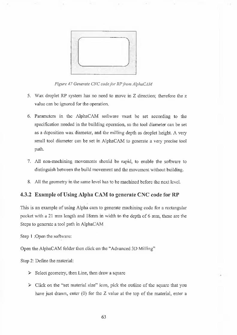
Y ^
V_____________________)
Figure 47 Generate CNC code for RP from AlphaCAM
5. Wax droplet RP system has no need to move in Z direction; therefore the z
value can be ignored for the operation.
6. Parameters in the AlphaCAM software must be set according to the
specification needed in the building operation, so the tool diameter can be set
as a deposition wax diameter, and the milling depth as droplet height. A very
small tool diameter can be set in AlphaCAM to generate a very precise tool
path.
7. All non-machining movements should be rapid, to enable the software to
distinguish between the build movement and the movement without building.
8. All the geometry in the same level has to be machined before the next level.
4.3.2 Example of Using Alpha CAM to generate CNC code for RP
This is an example of using Alpha cam to generate machining code for a rectangular
pocket with a 21 mm length and 18mm in width to the depth of 6 mm, these are the
Steps to generate a tool path in AlphaCAM
Step 1 :Open the software:
Open the AlphaCAM folder then click on the “Advanced 3D Milling”
Step 2: Define the material:
> Select geometry, then Line, then draw a square
> Click on the “set material size” icon, pick the outline of the square that you
have just drawn, enter (0) for the Z value at the top of the material, enter a
63

negative value less than -6 for the Z value at the bottom of the material, so
that the depth of material is greater than the depth o f the pocket.
Step 3 .'Define the shape to be machined
> Design the part: Size: 21 * 18 mm.
Step 4: Tool selection
> Click on the “Select” icon
> Scroll down the list and pick “Flat 3mm 2F EC HSS”
> Press enter to accept the tool.
Step 5. Tool Directions
> Select “CCW” for directions
> Select “Inside” for the Side.
r-Direction -Side------------------------------------------
Outside C Change Out/In L/R
(* |nsid^ Ç Centre
C Left C No Change
C Right C Automatic
C ÇW
<* CCW
C Reverse
C No Change
f~ Set Start Point on Closed Geometries
¿11 Geometries | Selected | Cancel
Figure 48 Tool Directions form in AlphaCAM software
Step 6. Pocketing: Click on the “Pocketing” icon
> Select “Vertical” for Sides
64
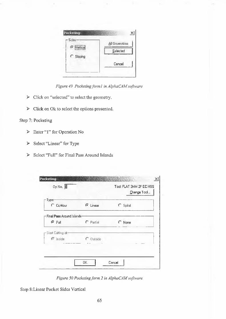
2£j
r SidesAll Geometries
Selected
Cancel
Figure 49 Pocketing form! in AlphaCAM software
> Click on “selected” to select the geometry.
> Click on Ok to select the options presented.
Step 7: Pocketing
> Enter “ 1” for Operation No
> Select “Linear” for Type
> Select “Full” for Final Pass Around Islands
x]
Op No. jn Tool: FLAT 3MM 2F ECHSSChange Tool...
r TypeC Contour <* Linear r Spiral
- Final Pass Around Islands
f? Full C Partial
-Start Cutting at
<* Inside
OK I Cancel
Figure 50 Pocketing form 2 in AlphaCAM software
Step 8:Linear Pocket Sides Vertical
65
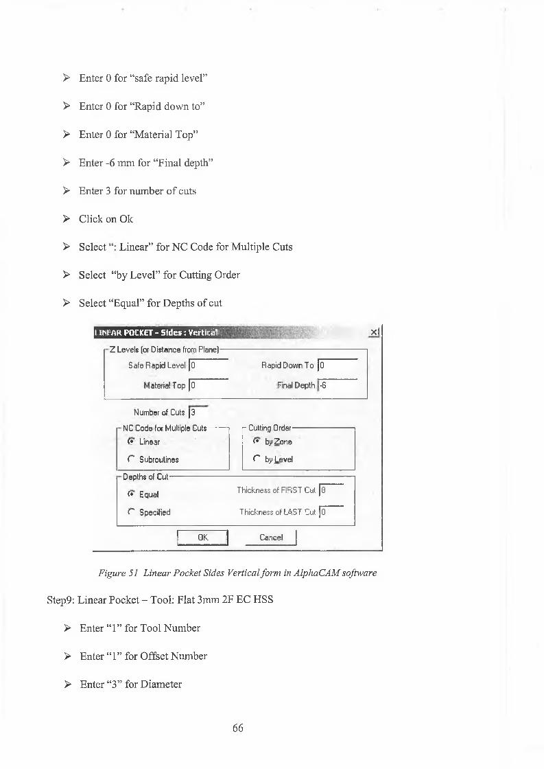
> Enter 0 for “safe rapid level”
> Enter 0 for “Rapid down to”
> Enter 0 for “Material Top”
> Enter -6 mm for “Final depth”
> Enter 3 for number o f cuts
> Click on Ok
> Select Linear” for NC Code for Multiple Cuts
> Select “by Level” for Cutting Order
> Select “Equal” for Depths of cut
s a a n sZ Levels (or Distance from Plane) -
Safe Rapid Level fo
Material Top [0
Rapid Down To fo"
Final Depth -S
xj
Number of Cuts |3
NC Code, for Multiple Cuts (* Linear
C Subroutines
Depths of Cut-
(* Equal
C Specified
OK
- Cutting Order- (* by Zone
r by Level
Thickness of FIRST Cut pT
Thickness of LAST Cut jo~
Cancel
Figure 51 Linear Pocket Sides Vertical form in AlphaCAM software
Step9: Linear Pocket - Tool: Flat 3mm 2F EC HSS
> Enter “1” for Tool Number
> Enter “ 1” for Offset Number
> Enter “3” for Diameter
66

> Enter “4000” for Spindle Speed
> Enter “ 10” for Down Feed
> Enter “20” for Cut Feed
> Enter “0” for Stock to be Left
> Enter “3” for Width, o f Cut = 3 mm
> Select “None” for Coolant
S H I i M U *J- T ooling--------------------------------------------------------------------------------
T ool N umber [i 0 ffset N umber fl
Diameter |3 Spindle Speed ¡4000
Down Feed }T6 Cut Feed [20
ividunii in lyStock to be Left |o Width of Cut |3j
uooiani
(* None C Mist f Flood C Through Tool
OK } Cancel
Figure 52 Linear Pocket - Tool: Flat 3mm 2FEC HSSform in AlphaCAM software
> Select Ok to select the options presented.
Step 10: Tool Path Resulted
> Click on the green geometry with the mouse.
> Click on finish.
CONTOUR POCKET - Tool: FLAT 3 M M 2F H?
67
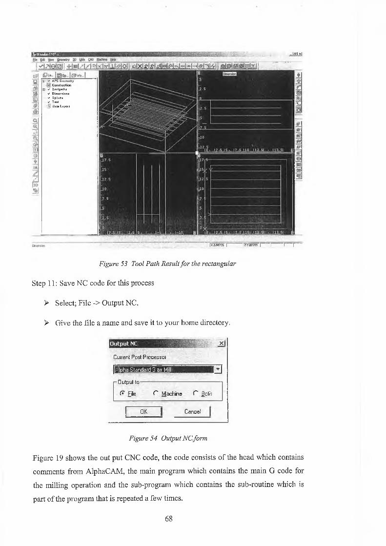
Jr St ond<ml Miti -Ifflxl
ffl'V APS Ceomsliy i_V Construction
CE v1 T o o lp a th s v* D im e ns ion s o' S p lin es ✓ T e x t
[0 User Layéis
ÌX3.99726 I II7.077S5 | I I f
Figure 53 Tool Path Result for the rectangular
Step 11: Save NC code for this process
> Select; File -> Output NC.
> Give the file a name and save it to your home directory.
x|
Current Post Processor
ElIpha Standard 3 ax Mill¡IrOutput to
(* File C Machine C Both
OK I Cancel
Figure 54 Output NCform
Figure 19 shows the out put CNC code, the code consists o f the head which contains
comments from AlphaCAM, the main program which contains the main G code for
the milling operation and the sub-program which contains the sub-routine which is
part of the program that is repeated a few times.
68
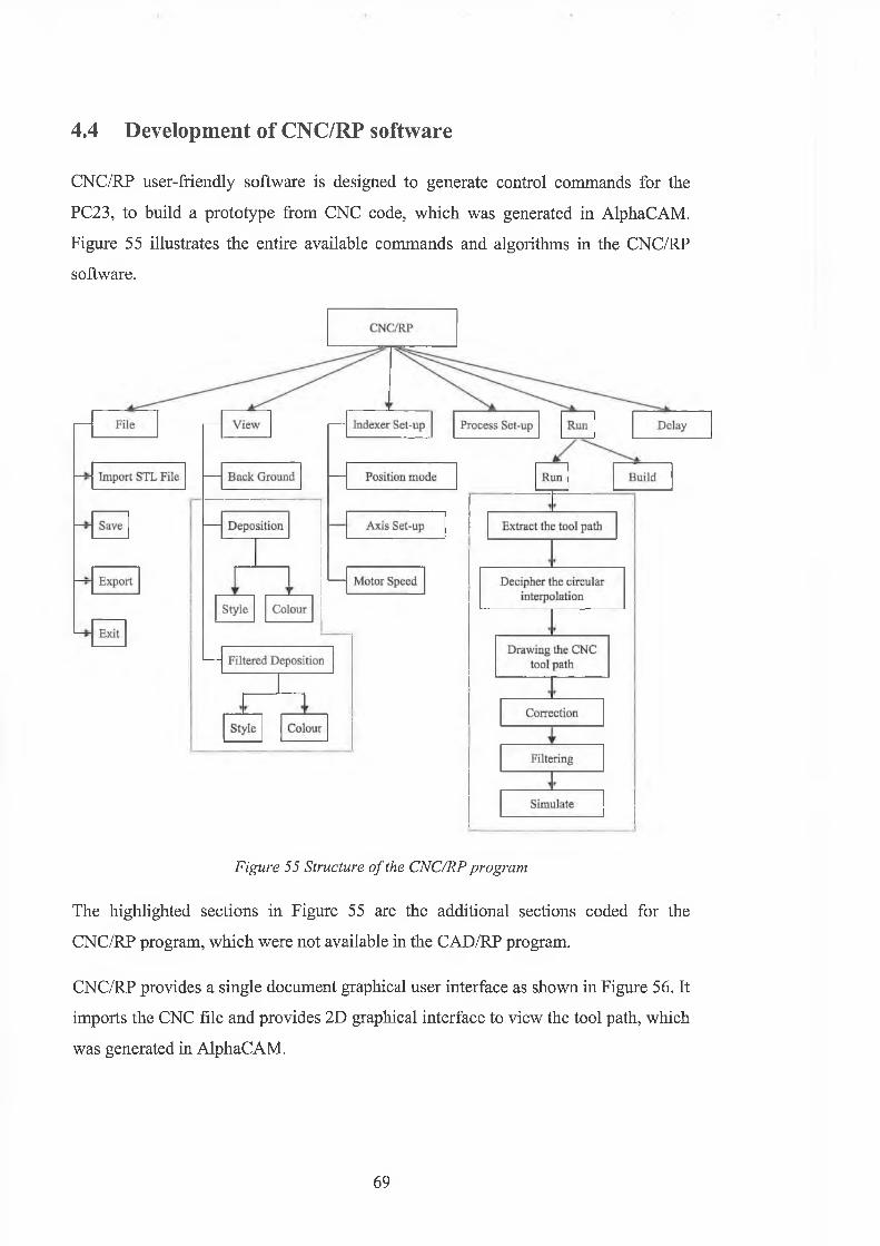
4.4 Development of CNC/RP software
CNC/RP user-friendly software is designed to generate control commands for the
PC23, to build a prototype from CNC code, which was generated in AlphaCAM.
Figure 55 illustrates the entire available commands and algorithms in the CNC/RP
software.
Figure 55 Structure o f the CNC/RP program
The highlighted sections in Figure 55 are the additional sections coded for the
CNC/RP program, which were not available in the CAD/RP program.
CNC/RP provides a single document graphical user interface as shown in Figure 56. It
imports the CNC file and provides 2D graphical interface to view the tool path, which
was generated in AlphaCAM.
69

Figure 56 Start-up screen
4.4.1 Import
The first step to processing any design is importing the CNC file code for the design,
CNC/RP imports the CNC file using import command from File menu see Figure 57
import command calls a common dialogue box to read the imported file name.
1 i , . C N C /R P - I n i * 1
1 File View I n d e x e r S e tu p P r o c e s s S e tu p R un D ela y
Im p o r t C tr l+ I
S a v e C tr l+ S
Exit
Figure 5 7 Import command.
4.4.2 View menu
CAD/RP provides capability to view the tool path and the simulation process in 2D
view, this gives the ability to insure that the right file is imported and the simulation is
acceptable before building the instruction command file. View menu contains sub
menus to view the deposition and filtered wax in different colours, see Figure 58.
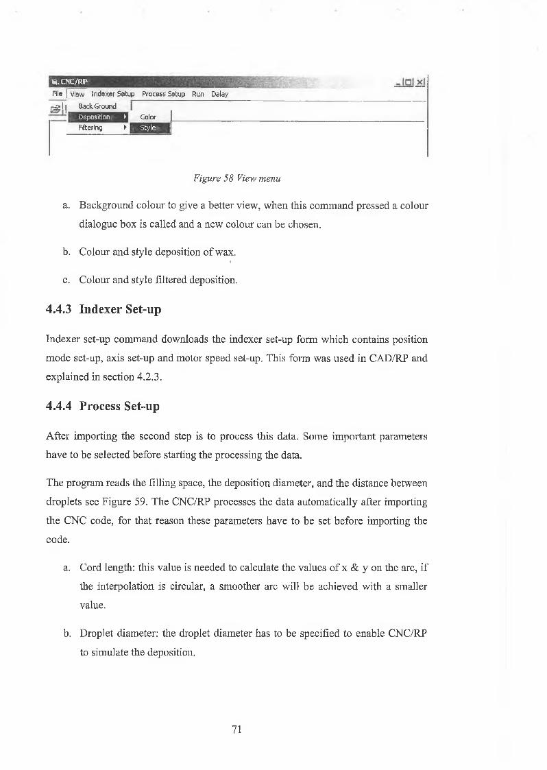
Si. CNC/RP
File | V iew I n d e x e r S e tu p P r o c e s s S e tu p R u n D elay
r ^ a l | B ack G ro u n d
D e p o s itio n ► C olor
F ilte rin g ► S ty le
Figure 58 View menu
a. Background colour to give a better view, when this command pressed a colour
dialogue box is called and a new colour can be chosen.
b. Colour and style deposition o f wax.i
c. Colour and style filtered deposition.
4.4.3 Indexer Set-up
Indexer set-up command downloads the indexer set-up form which contains position
mode set-up, axis set-up and motor speed set-up. This form was used in CAD/RP and
explained in section 4.2.3.
4.4.4 Process Set-up
After importing the second step is to process this data. Some important parameters
have to be selected before starting the processing the data.
The program reads the filling space, the deposition diameter, and the distance between
droplets see Figure 59. The CNC/RP processes the data automatically after importing
the CNC code, for that reason these parameters have to be set before importing the
code.
a. Cord length: this value is needed to calculate the values o f x & y on the arc, if
the interpolation is circular, a smoother arc will be achieved with a smaller
value.
b. Droplet diameter: the droplet diameter has to be specified to enable CNC/RP
to simulate the deposition.
71

c. Distance between the droplet: if this distance is not equal to the droplet
diameter it has to be specified to calculate the motor steps for each movement,
to generate the instruction commands for the PC23
-Jnj xj
- Chord Length----------------- -------------------- ----------------
Chord Lenght = J-j mm
by minimize this value, smaller steps will be calculated, which means smother curve will be obtained.
-Deposition Diameter-----------------------------------------------------------------
Deposition Diameter= mm
Deposition diameter is the diameter of the droplet of Wax, which is almost 3 mm
- Distance for deposition------------------------------
Distance between the droplets= J3 mm
1 Gk Cancel
Figure 59 Indexer set-up fcnm in CNC/RP program.
4.4.5 Processing Data
After the CNC file is imported, Run command can be executed by selecting the Run
button. The Run command executes four algorithms: (i) Extract, (ii) Draw, (iii)
Simulate and (iv) Correction. CNC/RP can execute these operations step by step from
Run menu by selecting each command button see Figure 60.
Process_Setupfrm
72

File V iew I n d e x e r S e t u p P r o c e s s S e t u p
Run command
Filtering command
Figure 60 Rum menu
When CNC/RP is executed the program opens the selected CNC file as a sequential
input file, reads the text line-by-line, extracts all needed information such as G codes,
the displacements in x, y, z and R, manipulates the tool path, simulates the deposition
o f wax, filtering the additional deposition in some areas, and then translates the CNC
code to X-language codes, which are the PC23 indexer instructions to drive the
motors.
The program flow is divided into seven steps:
1. Extract the tool path.
2. Drawing the CNC tool path.
3. Simulate.
4. Correction.
5. Filtering.
6. Build the instruction command file for PC23
7. Save
73
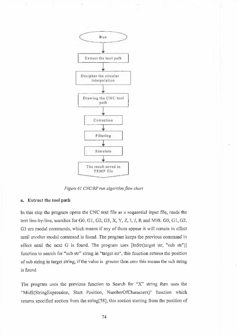
Run
Figure 61 CNC/RF run algorithm flow chart
a. Extract the tool path
In this step the program opens the CNC text file as a sequential input file, reads the
text line-by-line, searches for GO, G l, G2, G3, X, Y, Z, I, J, R and M98. GO, G l, G2,
G3 are modal commands, which means if any of them appear it will remain in effect
until another modal command is found. The program keeps the previous command in
effect until the next G is found. The program uses [InStr(target str, "sub str")]
function to search for “sub str” string in “target str", this function returns the position
of sub string in target string, if the value is greater then zero this means the sub string
is found
The program uses the previous function to Search for “X ” string then uses the
“Mid$(StringExpression, Start Position, NumberOfCharacters)" function which
returns specified section from the string[58]; this section starting from the position of
74
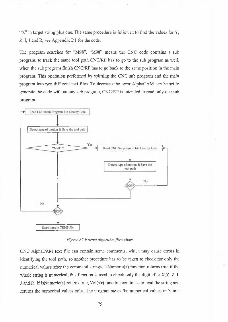
“X ” in target string plus one. The same procedure is followed to find the values for Y,
Z, I, J and R, see Appendix D1 for the code.
The program searches for “M98”. “M98” means the CNC code contains a sub
program, to track the same tool path CNC/RP has to go to the sub program as well,
when the sub program finish CNC/RP has to go back to the same position in the main
program. This operation performed by splitting the CNC sub program and the main
program into two different text files. To decrease the error AlphaCAM can be set to
generate the code without any sub program, CNC/RP is intended to read only one sub
program.
Figure 62 Extract algorithm flow chart
CNC AlphaCAM text file can contain some comments, which may cause errors in
identifying the tool path, so another procedure has to be taken to check for only the
numerical values after the command strings. IsNumeric(a) function returns true if the
whole string is numerical, this function is used to check only the digit after X,Y, Z, I,
J and R. If IsNumeric(a) returns true, Val(str) function continues to read the string and
returns the numerical values only. The program saves the numerical values only in a
75
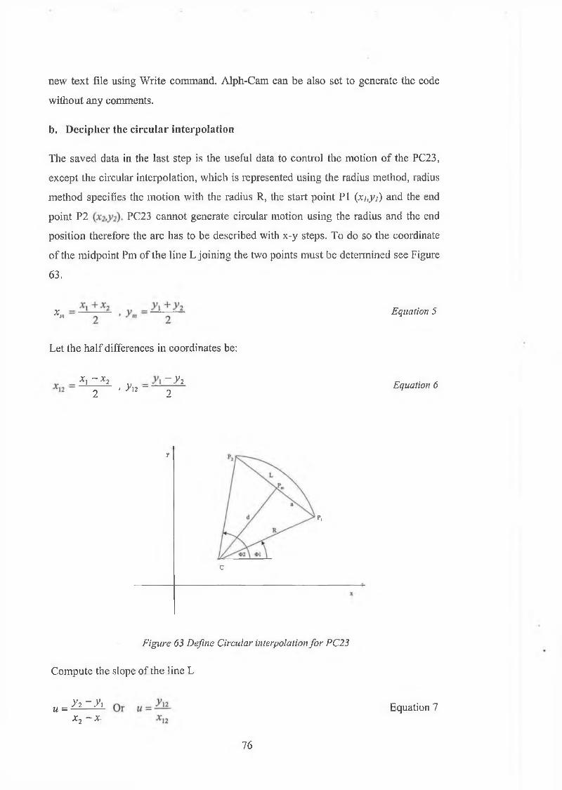
new text file using Write command. Alph-Cam can be also set to generate the code
without any comments.
b. Decipher the circular interpolation
The saved data in the last step is the useful data to control the motion of the PC23,
except the circular interpolation, which is represented using the radius method, radius
method specifies the motion with the radius R, the start point PI (xi.yi) and the end
point P2 PC23 cannot generate circular motion using the radius and the end
position therefore the arc has to be described with x-y steps. To do so the coordinate
o f the midpoint Pm of the line L joining the two points must be determined see Figure
63.
x,lit Equation 5
Let the half differences in coordinates be:
* l - * 2 .. - ^ 2 2 ■ y n ~ 2
Equation 6
y
p,
c
Figure 63 Define Circular interpolation for PC23
Compute the slope of the line L
u = >'2 “ .VlX 2 ~ X \
Equation 7
76
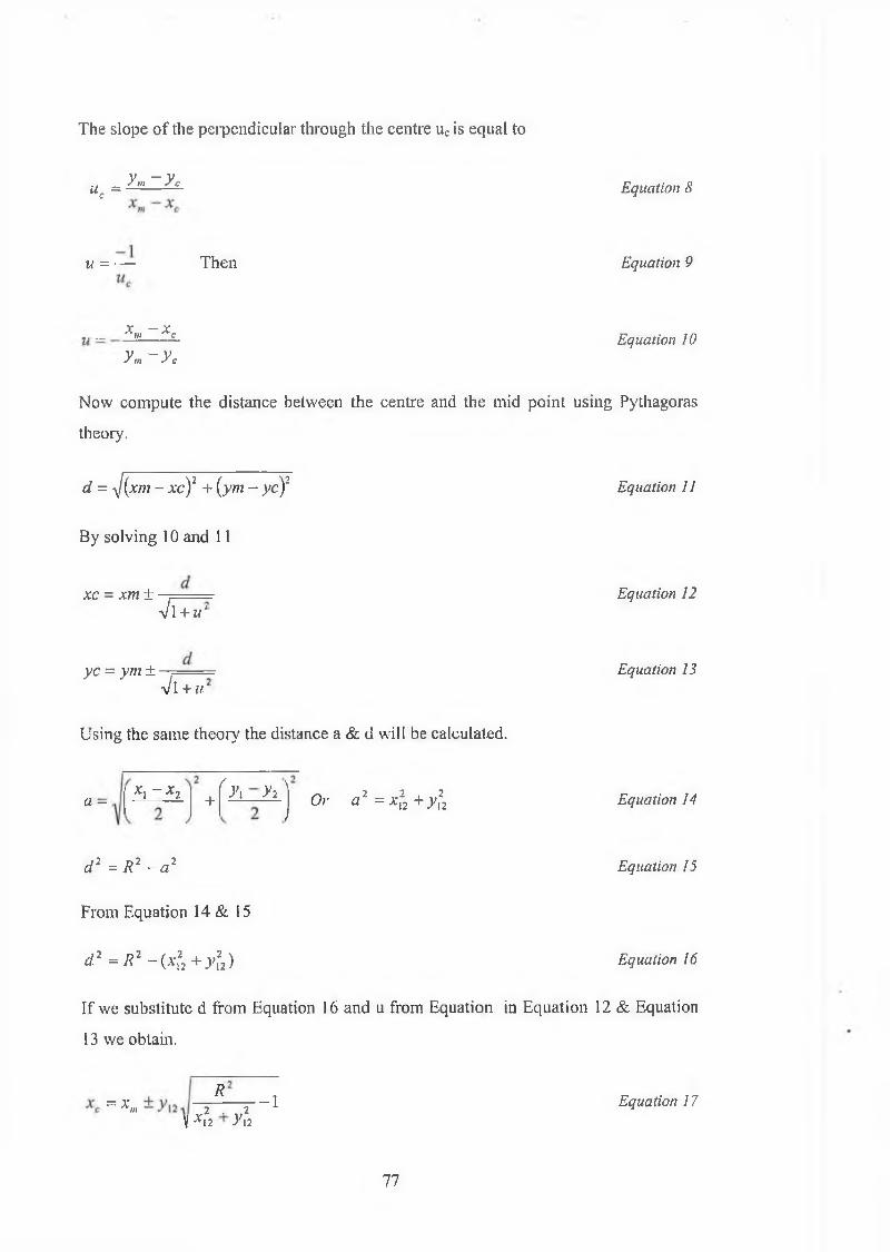
The slope o f the perpendicular through the centre uc is equal to
ue = y* ~yc Equation 8
u = —- Then Equation 9
. . . . X m ~ X c
ym ~ycEquation 10
Now compute the distance between the centre and the mid point using Pythagoras
theory.
d = yj(xm - a x ' ) 2 + (ym - yc)2 Equation II
By solving 10 and 11
xc = xm ±V1 + u i
Equation 12
yc = ym ±Vl + « ;
Equation 13
Using the same theory the distance a & d will be calculated.
a -x, - x 2 + f A _ A | o r a 2 = xf2 + y f2 Equation 14
d 2 = R 2 - a 2 Equation 15
From Equation 14 & 15
d 2 = R 2 - { x f 2 + y f 2) Equation ¡6
If we substitute d from Equation 16 and u from Equation in Equation 12 & Equation
13 we obtain.
*=*», 2 ■ 2
v x i2 yn- i Equation 17
11

\ *12 + 312y c = y m ±*12 Equation 18
Figure 64 Circular interpolation
These two equations will give two centres. For each centre two possible arcs are
possible. In general, the problem of joining two points with an arc o f a given radius
has four solutions: Clockwise interpolation with long or short arc, counter clockwise
interpolation with short or long arc [59].
To perceive the long and the short arcs, the angle <t>, formed by the line joining the
start point and the centre with the x-axis, and the angle 0 2 formed by the line joining
the end point and the centre with the x-axis, see Figure 63, will be calculated for each
centre, using the atan2 function which returns an angel between 0 and 27T. Visual
Basic does not compile atan2 function, the author proposed a similar function to
return a similar value see Appendix D2.
Equatim I9x lc = x2- x c y ^ = y , - y .
See Figure 63
78
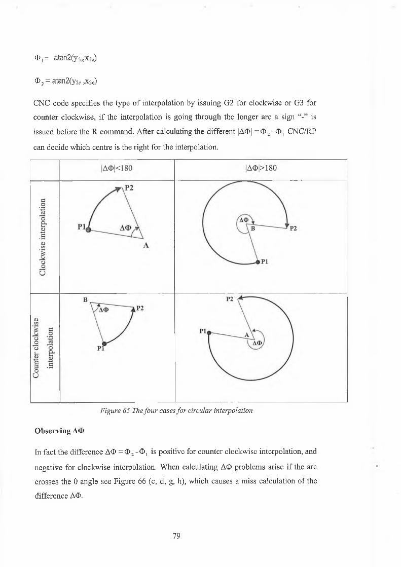
$ != atan2(ylc,xic)
i>2 = atan2(y2c ,x2c)
CNC code specifies the type o f interpolation by issuing G2 for clockwise or G3 for
counter clockwise, if the interpolation is going through the longer arc a sign is
issued before the R command. After calculating the different |AO| = 0 2-Oj CNC/RP
can decide which centre is the right for the interpolation.
Figure 65 The four cases for circular interpolation
Observing AO
In fact the difference AO = 0 2 - 0 [ is positive for counter clockwise interpolation, and
negative for clockwise interpolation. When calculating AO problems arise if the arc
crosses the 0 angle see Figure 66 (c, d, g, h), which causes a miss calculation of the
difference AO.
79
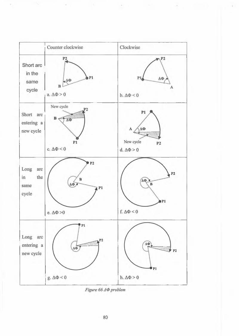
80
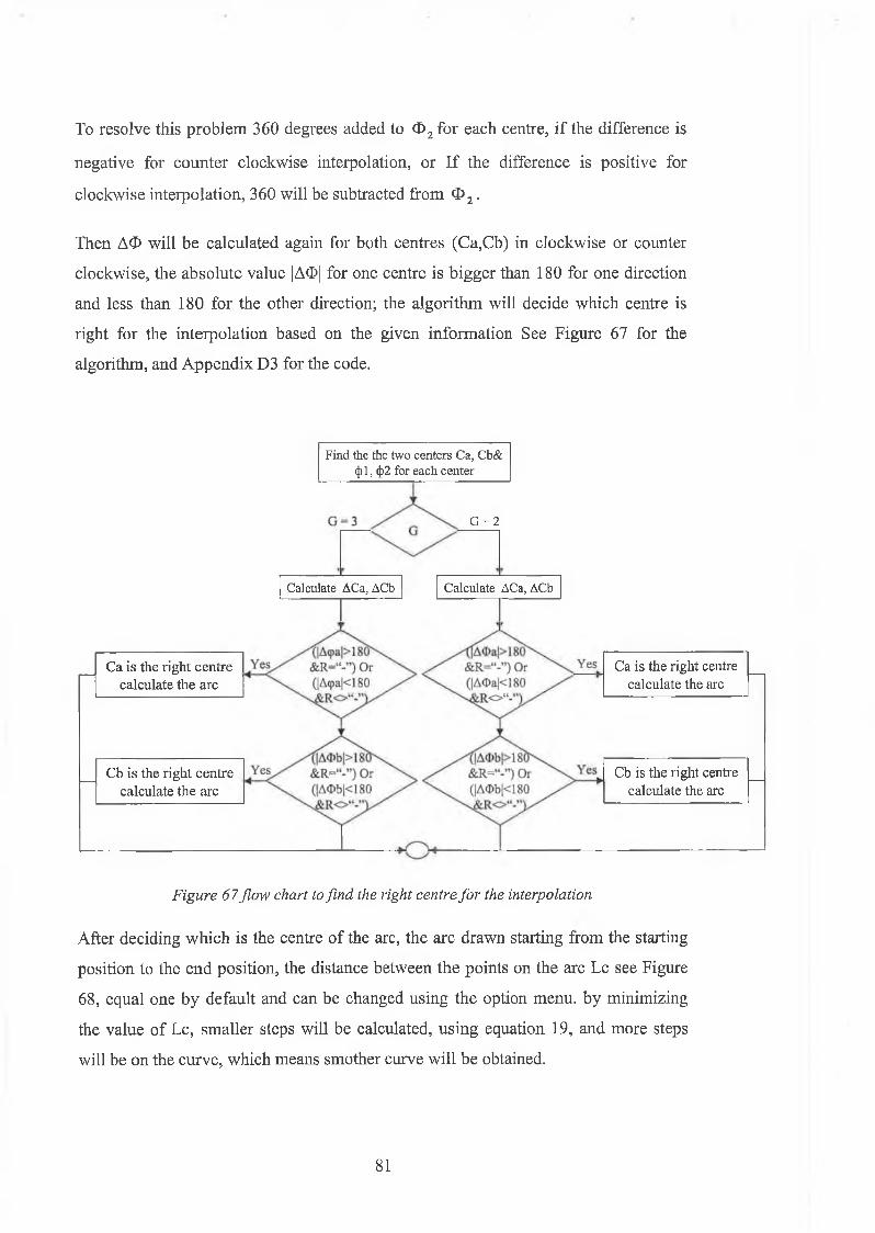
To resolve this problem 360 degrees added to 0 2 for each centre, if the difference is
negative for counter clockwise interpolation, or I f the difference is positive for
clockwise interpolation, 360 will be subtracted from 0 2.
Then AO will be calculated again for both centres (Ca,Cb) in clockwise or counter
clockwise, the absolute value |AO| for one centre is bigger than 180 for one direction
and less than 180 for the other direction; the algorithm will decide which centre is
right for the interpolation based on the given information See Figure 67 for the
algorithm, and Appendix D3 for the code.
Find the the two centers Ca, Cb& (Jjl, <J>2 for each center
G = 2
Ca is the right centre calculate the arc
Cb is the right centre calculate the arc
Ca is the right centre calculate the arc
Cb is the right centre calculate the arc
Calculate ACa, ACb Calculate ACa, ACb
Figure 67 flow chart to find the right centre for the interpolation
After deciding which is the centre of the arc, the arc drawn starting from the starting
position to the end position, the distance between the points on the arc Lc see Figure
68, equal one by default and can be changed using the option menu, by minimizing
the value of Lc, smaller steps will be calculated, using equation 19, and more steps
will be on the curve, which means smother curve will be obtained.
81

2
1
0
Figure 68 chord length for one step angle
180 Lcstep = ----------tvR
Equation 20
Where Lc is the chord length for one step angle.
c. Drawing the CNC Tool Path
To draw on the screen, first the screen has to be scaled, using the max values for x and
y, the program reads “outfile3”file which contains the entire tool path in linear
displacement only and draws the tool path on the screen using the line command
{Picturel.Line (x l, yl)-(x2, y2)} see Appendix D4 for the code. This will give the
operator the chance to check if there are any mistakes in reading the CNC code. If the
result is satisfied the operator continue to the next step.
d. Simulate
To simulate the deposition o f wax the algorithm start by opening the “outfile3”. The
program reads G, X, and Y computes the total displacements in x and y direction then
calculates the total travelling distance Dt .
Dx - x2 - x , Equation 21
Dy — y 2 ~y\ Equation 22
Equation 23
82
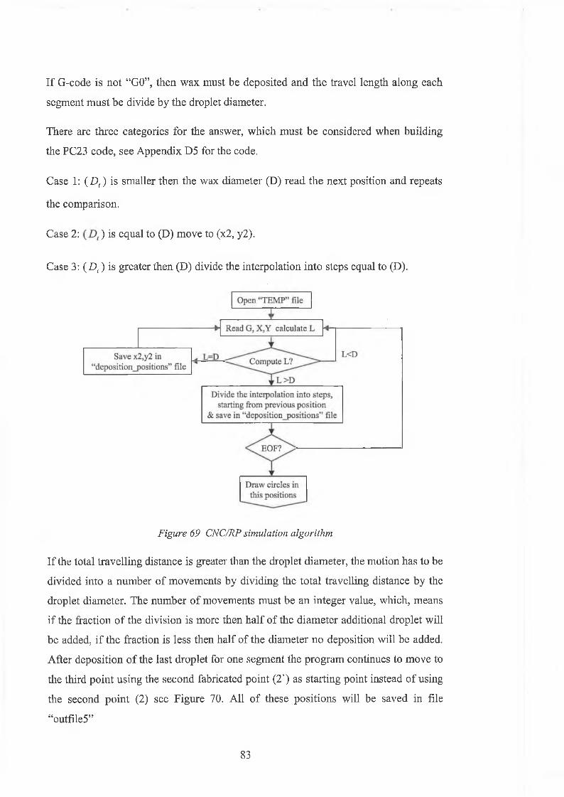
I f G-code is not “GO”, then wax must be deposited and the travel length along each
segment must be divide by the droplet diameter.
There are three categories for the answer, which must be considered when building
the PC23 code, see Appendix D5 for the code.
Case 1: ( D t ) is smaller then the wax diameter (D) read the next position and repeats
the comparison.
Case 2: ) is equal to (D) move to (x2, y2).
Case 3: ( D , ) is greater then (D) divide the interpolation into steps equal to (D).
Figure 69 CNC/RP simulation algorithm
If the total travelling distance is greater than the droplet diameter, the motion has to be
divided into a number of movements by dividing the total travelling distance by the
droplet diameter. The number o f movements must be an integer value, which, means
if the fraction of the division is more then half of the diameter additional droplet will
be added, if the fraction is less then half of the diameter no deposition will be added.
After deposition o f the last droplet for one segment the program continues to move to
the third point using the second fabricated point (2') as starting point instead of using
the second point (2) see Figure 70. All of these positions will be saved in file
“outfile5”
83

CNC tool path
Error
(a) an extra droplet deposited
Figure 70 Error due to moving from fabricated point
e. Correction:
It is noted that some of the voids and geometric errors will accrue using the above
technique. This problem can be avoided by starting the new movement from the new
position (2), not from the fabricated point (2 ') see Figure 71. The program simulates
the deposition of wax after correcting the path. See Appendix D5 for the code.
Figure 71 Starting the new movement from the original last position
84
f. Filtering.
A Filtering operation can be executed by selecting “Filter” command from Run menu
or by clicking on filter button Figure 60. Filtering operation is performed to eliminate
the additional deposition of material. Filtering can be done with different factors.
Increasing this value will eliminate more deposition points.
The process proceeds by transferring the first point from “outfile5” file into
“outfile6”, then picking the next point from “outfile5” and determine the distance
between this point and the previous points in “outfile6”, if the distance is bigger than
the checking value the program will save this point in “outfile6”, if not the program
omitt this point. The program continues to check all the deposition positions by
scanning “outfile6” for each point in “outfile5”, CNC/RP simulates the omitted points
in different colour on the screen see Appendix D6 for the code.
g. Build the instruction command file for PC23
Build operation can be executed by selecting “Build” command from Run see Figure
60. Build command builds the instruction commands in X-language to operate PC23
indexer. The instruction command will be formulated according to the last function
(simulate, correction or filtering)
The same algorithm in CAD/RP programme is used here, see section 0.
h. Save
The Save command from file the menu will call the save dialogue box to save the
command strings file in a text file. The same form was also used in CAD/RP see 0
85
Chapter 5 Result And Discussion
This chapter is devoted to the analysis and discussion of the outcomes and
performance of the developed software. Section 5.1 describes CAD/RP capabilities
and all the required steps to generate the RP instructions command file. Section 5.2
describes CNC/RP software capabilities and its performance. Section Error!
Reference source not found, illustrate the development in the CAM/RP program
which controls the wax depositing RP system. Many parts were fabricated using this
wax droplet RP system using the data obtained from CNC/RP.
5.1 CAD/RP
CAD/RP proved the capability to process and slice STL files, generate the tool path
for RP operation and constructs the instruction commands for the PC indexer. The
entire progress through the steps can be visually displayed and controlled in CAD/RP.
5.1.1 View Geometry
CAD/RP provides capability to view the design in 2D and 3D. This gives the ability
to ensure that the right design is imported before starting the slicing process. CAD/RP
views the model in x-y, x-z, y-z and 3D coordinate systems, see Figure 72.
86
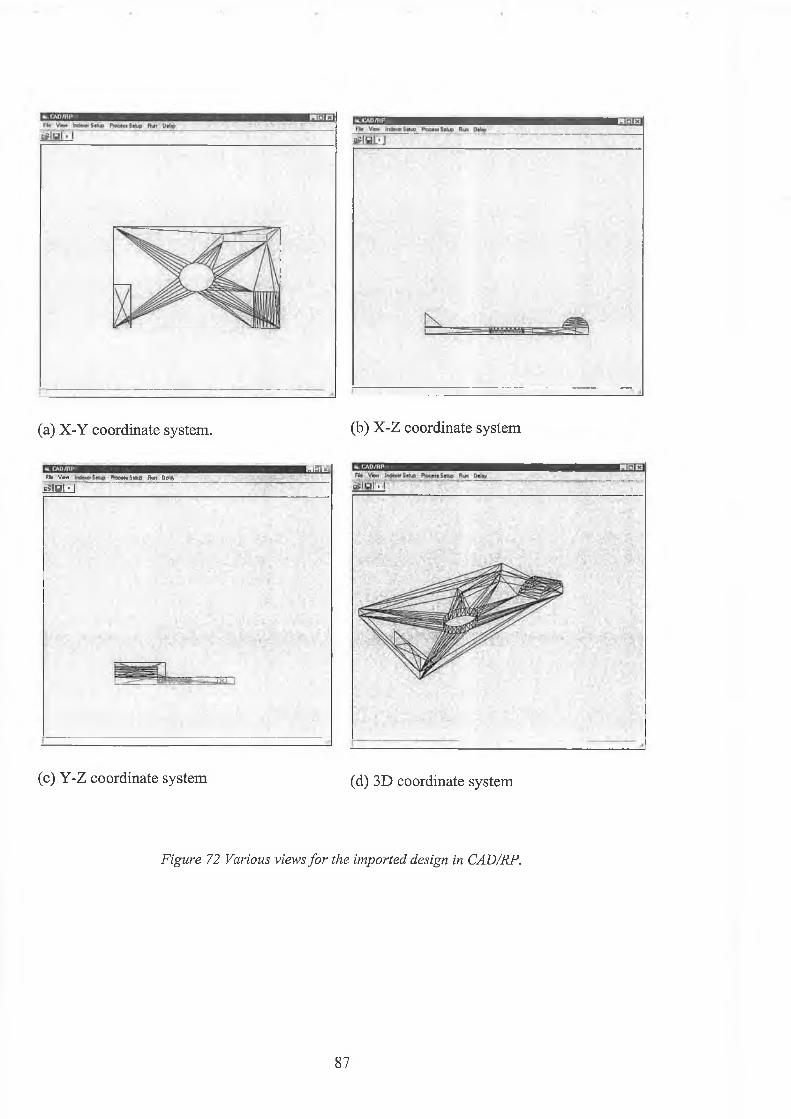
(a) X-Y coordinate system. (b) X-Z coordinate system
w - i n lfit v»n P-ocan Saq fkn Vtltrg» i q i • i
(c) Y-Z coordinate system (d) 3D coordinate system
the imported design in CAD/RP.Figure 72 Various views for
87

5.1.2 Slicing process
CAD/RP is capable of slicing any STL file with any layer thickness. The result of this
operation is a random segment order contour. When a long delay time is specified a
random construction of the contour can be observed see Figure 73.
(a) 25% of contour
E S H T .L v '- ;:
(c) 75% of contour
(b) 50% of contour
n*°*iai • i
h lti* Wsp Ak iii SHip hn Miy
(d) 100% of contour
Figure 73 Construction o f contour as found in STL file
88
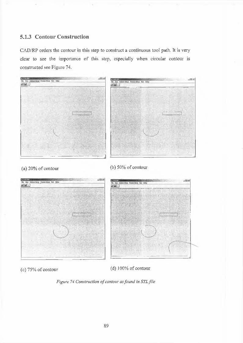
5.1.3 Contour Construction
CAD/RP orders the contour in this step to construct a continuous tool path. It is very
clear to see the importance o f this step, especially when circular contour is
constructed see Figure 74.
(a) 20% of contour (b) 50% of contour
(c) 75% of contour (d) 100% of contour
Figure 74 Construction o f contour as found in STL file
89
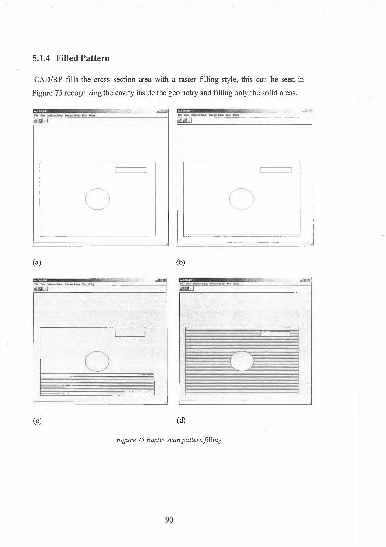
5.1.4 Filled Pattern
CAD/RP fills the cross section area with a raster filling style, this can be seen in
Figure 75 recognizing the cavity inside the geometry and filling only the solid areas.
(a) (b)
(c) (d)
Figure 75 Raster scan pattern filling
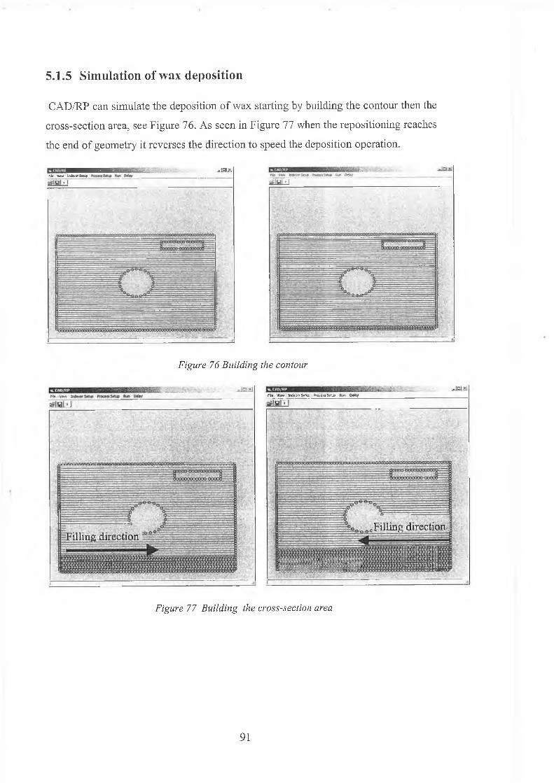
Figure 7(5 Building the contour
CAD/RP can simulate the deposition of wax starting by building the contour then the
cross-section area, see Figure 76. As seen in Figure 77 when the repositioning reaches
the end of geometry it reverses the direction to speed the deposition operation.
5.1.5 Simulation of wax deposition
__ -amirit < « • I n t e v h M __ ____________
illing direction
««••«tas99ets*t»s9(9oes9»o99?9e■oiotcco 99:019c»9«cei»»#»03' S S S i S g g S S S l M i g S S S S S S : Z i S S M f X i.3;;:s>3;s_ca»_a>.»la e <«»»>-»>-»
Fifl. Vlsw Indexer f-'.'vj fi [Vf-1i iftKB ftW) WAf
F illin g direction
Figure 77 Building the cross-section area
91
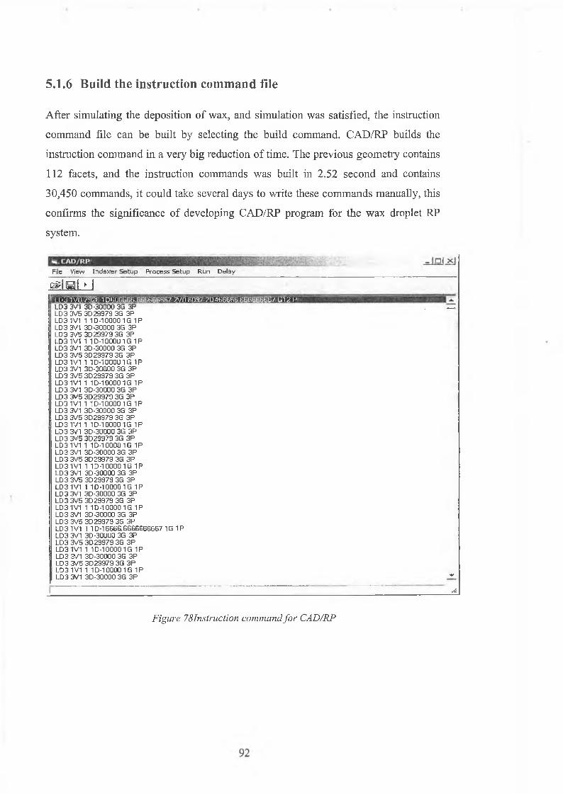
5.1.6 Build the instruction command file
After simulating the deposition o f wax, and simulation was satisfied, the instruction
command file can be built by selecting the build command. CAD/RP builds the
instruction command in a very big reduction of time. The previous geometry contains
112 facets, and the instruction commands was built in 2.52 second and contains
30,450 commands, it could take several days to write these commands manually, this
confirms the significance of developing CAD/RP program for the wax droplet RP
system.
File View Indexer Setup Process Setup Run Delayb»I'b I ► Si LD31 V0.792G 10606666.666666667 2VÛ.6097 20466666.666666667 ÜÏ2 PLD3 3VI 3D-30000 3G 3P ___LD3 3V5 3D29979 3G 3PLD3 1V1 1 1D-10000 1G 1PLD3 3V1 3D-30000 3G 3PLD3 3V5 3D 29979 3G 3PLD31V1 1 1D-100001G 1PLD3 3V1 3D-30000 3G 3PLD3 3V5 3D29979 3G 3PLD31V1 1 1D-100001G 1PLD3 3V1 3D-30000 3G 3PLD3 3V5 3D 23373 3G 3PLD31V1 1 1D-100001G 1PLD3 3V1 3D-30000 3G 3PLD3 3V5 3D29979 3G 3PLD31V1 1 1D-10000 1G 1PLD3 3V1 3D-30000 3G 3PLD3 3V5 3D 29979 3G 3PLD31V1 1 1D-100001G 1PLD3 3V1 3D-30000 3G 3PLD3 3V5 3D29979 3G 3PLD31V1 1 1D-10000 1G 1PLD3 3V1 3D-30000 3G 3PLD3 3V5 3D 29979 3G 3PLD31V1 1 1D-100001G 1PLD3 3V1 3D-30000 3G 3PLD3 3V5 3D29979 3G 3PLD31V1 1 ID-10000 1 G 1PLD3 3V1 3D-30000 3G 3PLD3 3V5 3D23373 3G 3PLD31V1 1 1D-1Ü0001G 1PLD3 3V1 3D-30000 3G 3PLD3 3V5 3D 29979 3G 3PLD31V1 1 1D-16666.6666666667 1G 1PLD3 3V1 3D-30000 3G 3PLD3 3V5 3D29979 3G 3PLD31V1 1 1D-100001G 1PLD3 3V1 3D-30000 3G 3PLD3 3V5 3D 29979 3G 3PLD31V1 1 1D-10000 1G 1P
l LD3 3V1 3D-30000 3G 3P 'V
A
Figure 78Instruction command for CAD/RP
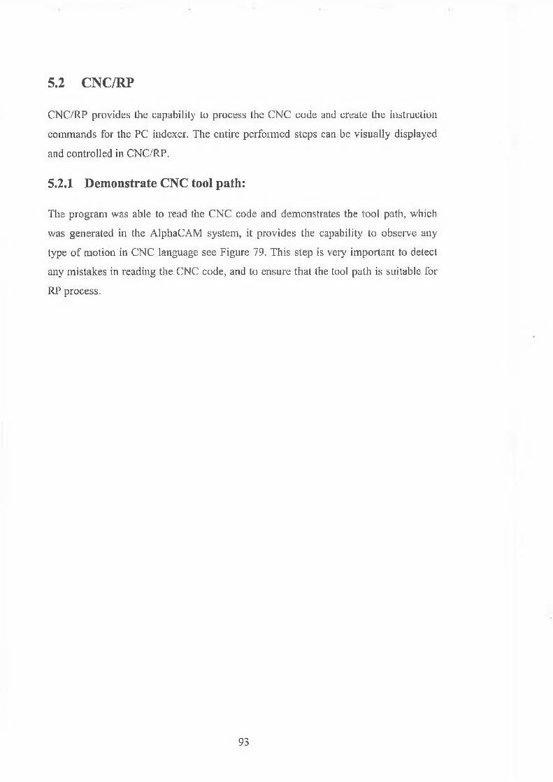
5.2 CNC/RP
CNC/RP provides the capability' to process the CNC code and create the instruction
commands for the PC indexer. The entire performed steps can be visually displayed
and controlled in CNC/RP.
5.2.1 Demonstrate CNC tool path:
The program was able to read the CNC code and demonstrates the tool path, which
was generated in the AlphaCAM system, it provides the capability to observe any
type o f motion in CNC language see Figure 79. This step is very important to detect
any mistakes in reading the CNC code, and to ensure that the tool path is suitable for
RP process.
93
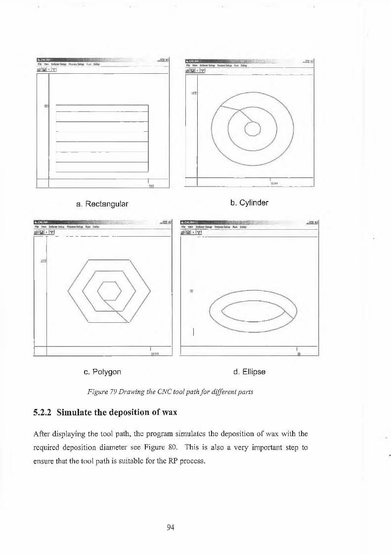
a. Rectangular b. Cylinder
c. Polygon d. Ellipse
Figure 79 Drawing the CNC tool path for different parts
5.2.2 Simulate the deposition of wax
After displaying the tool path, the program simulates the deposition of wax with the
required deposition diameter see Figure 80. This is also a very important step to
ensure that the tool path is suitable for the RP process.
94
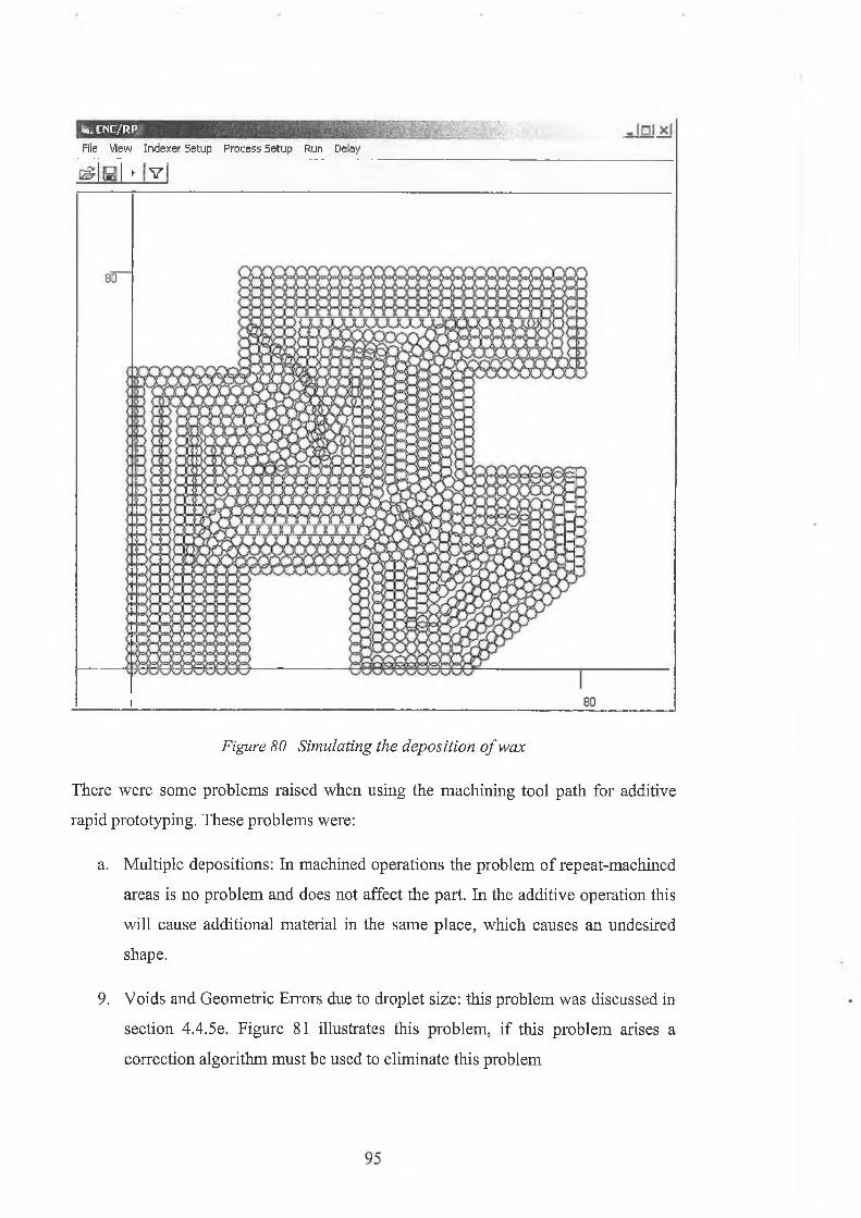
fei* CNC/RP
File V iew I n d e x e r S e tu p P r o c e s s S e tu p R un D elay
► V
Figure 80 Simulating the deposition o f wax
There were some problems raised when using the machining tool path for additive
rapid prototyping. These problems were:
a. Multiple depositions: In machined operations the problem of repeat-machined
areas is no problem and does not affect the part. In the additive operation this
will cause additional material in the same place, which causes an undesired
shape.
9. Voids and Geometric Errors due to droplet size: this problem was discussed in
section 4.4.5e. Figure 81 illustrates this problem, if this problem arises a
correction algorithm must be used to eliminate this problem

m m k jjDfjilFile View. Indexer Setup Process Setup Run Delay
{5r O V
Additionaldeposition
Voids
GeometrieError
Figure 81 Figure 81 Voids and Geometric Errors
5.2.3 Correction
It is noted that some of the Voids and Geometric Errors, which mentioned above,
could be avoided by using correction algorithm see 4.4.5e. Figure 83 show the
simulation after correcting the paths.
96
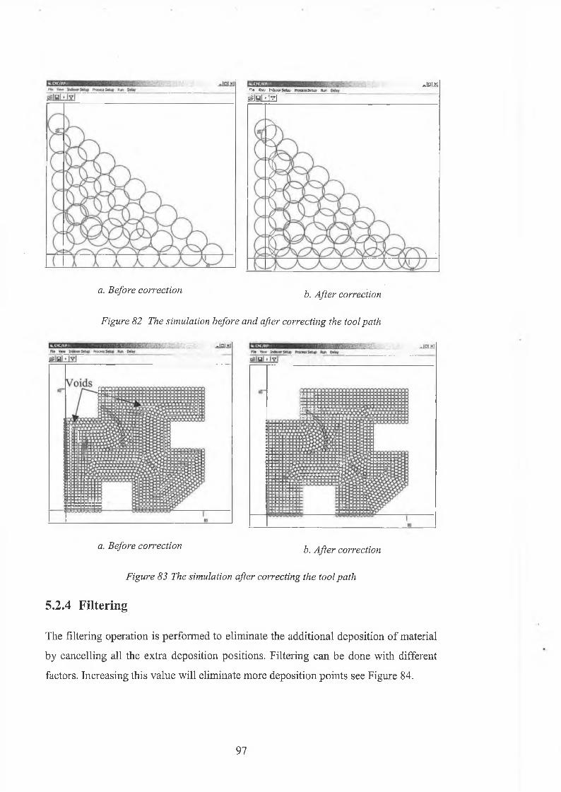
Fifa Vtew f a k a r Stìxp ìv x tn 5 itip Ryn
¿¡sLdzf*!0!*J
a. Before correction b. After correction
Figure 82 The simulation before and after correcting the tool path
a. Before correction b. After correction
Figure 83 The simulation after correcting the tool path
5.2.4 Filtering
The filtering operation is performed to eliminate the additional deposition o f material
by cancelling all the extra deposition positions. Filtering can be done with different
factors. Increasing this value will eliminate more deposition points see Figure 84.
97
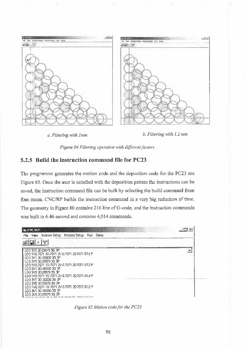
a. Filtering with 1mm b. Filtering with 1.2 mm
Figure 84 Filtering operation with different factors
5.2.5 Build the instruction command file for PC23
The programme generates the motion code and the deposition code for the PC23 see
Figure 85. Once the user is satisfied with the deposition pattern the instructions can be
saved, the instruction command file can be built by selecting the build command from
Run menu. CNC/RP builds the instruction command in a very big reduction of time.
The geometry in Figure 80 contains 216 line of G-code, and the instruction commands
was built in 6.46 second and contains 4,014 commands.
CNC/RP ... ........... -ini xjFile View I n d e x e r S e tu p P ro c e s s S e tu p R u n D elay
yLD 3 3V 5 3 D 2 9 9 7 9 3G 3 P ............ "L D 3 1 VO. 7071 1D -7071 2V -Ü.7071 2D 7071 G 1 2 PLD 3 3V1 3 D -3 0 0 0 0 3G 3PL D 3 3V 5 3D 2 9 9 7 9 3G 3 PL D 3 1 V 0 .7071 1D -7071 2V -0 .7071 2 D 7 0 7 1 G 1 2 PLD 3 3V1 3 D -3 0 0 0 0 3G 3PL D 3 3V 5 3D 2 9 9 7 9 3G 3 PL D 3 1V 0 .7071 1D -7071 2V -0 .7071 2D 7 0 7 1 G 1 2 PLD 3 3V1 3 D -3 0 0 0 0 3G 3 PLD 3 3V 5 3D 2 9 9 7 9 3G 3 PL D 3 1 V 0 .7 0 7 1 1D -7071 2V -0 .7071 2D 7071 G 1 2 PL D 3 3V1 3 D -3 0 0 0 0 3G 3PLD 3 3 ^ 5 3 D 2 9 9 7 9 3G 3 P
Figure 85 Motion code for the PC23
98
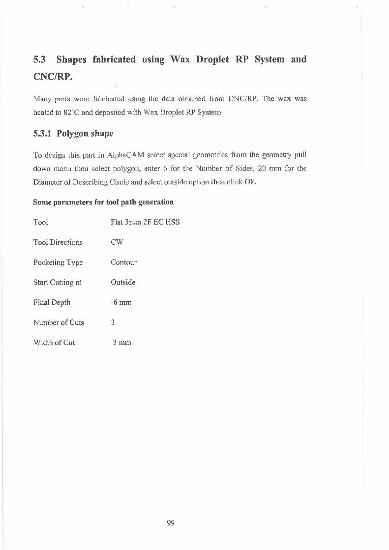
5.3 Shapes fabricated using Wax Droplet RP System and
CNC/RP.
Many parts were fabricated using the data obtained from CNC/RP, The wax was
heated to 82°C and deposited with Wax Droplet RP System.
5.3.1 Polygon shape
To design this part in AlphaCAM select special geometries from the geometry pull
down menu then select polygon, enter 6 for the Number o f Sides, 20 mm for the
Diameter of Describing Circle and select outside option then click Ok.
Some parameters for tool path generation
Tool Flat 3mm 2F EC HSS
Tool Directions CW
Pocketing Type Contour
Start Cutting at Outside
Final Depth -6 mm
Number o f Cuts 3
Width of Cut 3 mm
99
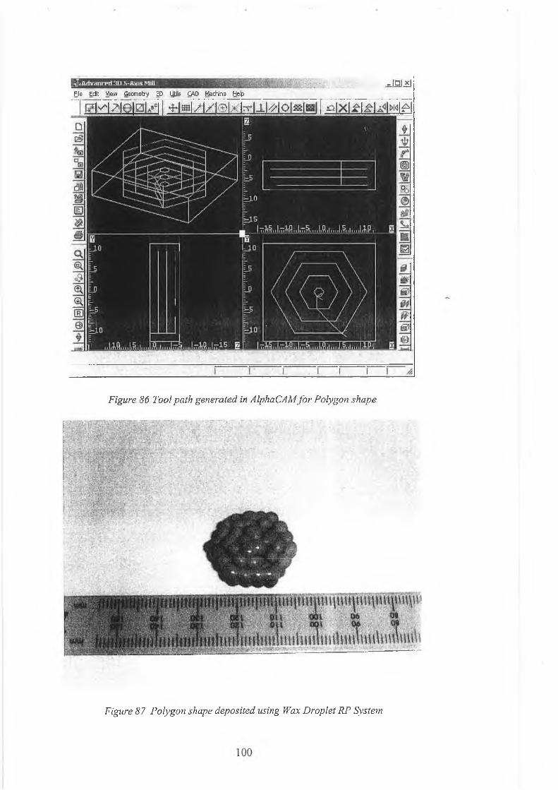
File Edit View Geometry 3D Utils CAD Machine Help
Figure 86 Tool path generated in AlphaCAM for Polygon shape
*>!.
f W - V
Figure 87 Polygon shape deposited using Wax Droplet RP System

5.3.2 Ellipse shape
Select special geometries in AlphaCAM from geometry pull down menu then select
polygon, enter 25 for the Width, 15 mm for Height, 4 for the Number of Quadrants
and 4 for the Number of Arcs per Quadrant, then click Ok.
Some parameters for tool path generation
Tool
Tool Directions
Pocketing Type
Start Cutting at
Final Depth
Number of Cuts
Width of Cut
Flat 3mm 2F EC HSS
CW
Contour
Outside
-6 mm
3
3 mm
Advanced 3D 5-Axis Mill
File Edit View G eom etry 3D Utils £AD M achine Help
Figure 88 Tool path generated in AlphaCAM for an Ellipse shape
101

Figure 89 Ellipse shape deposited using Wax Droplet RP System
102
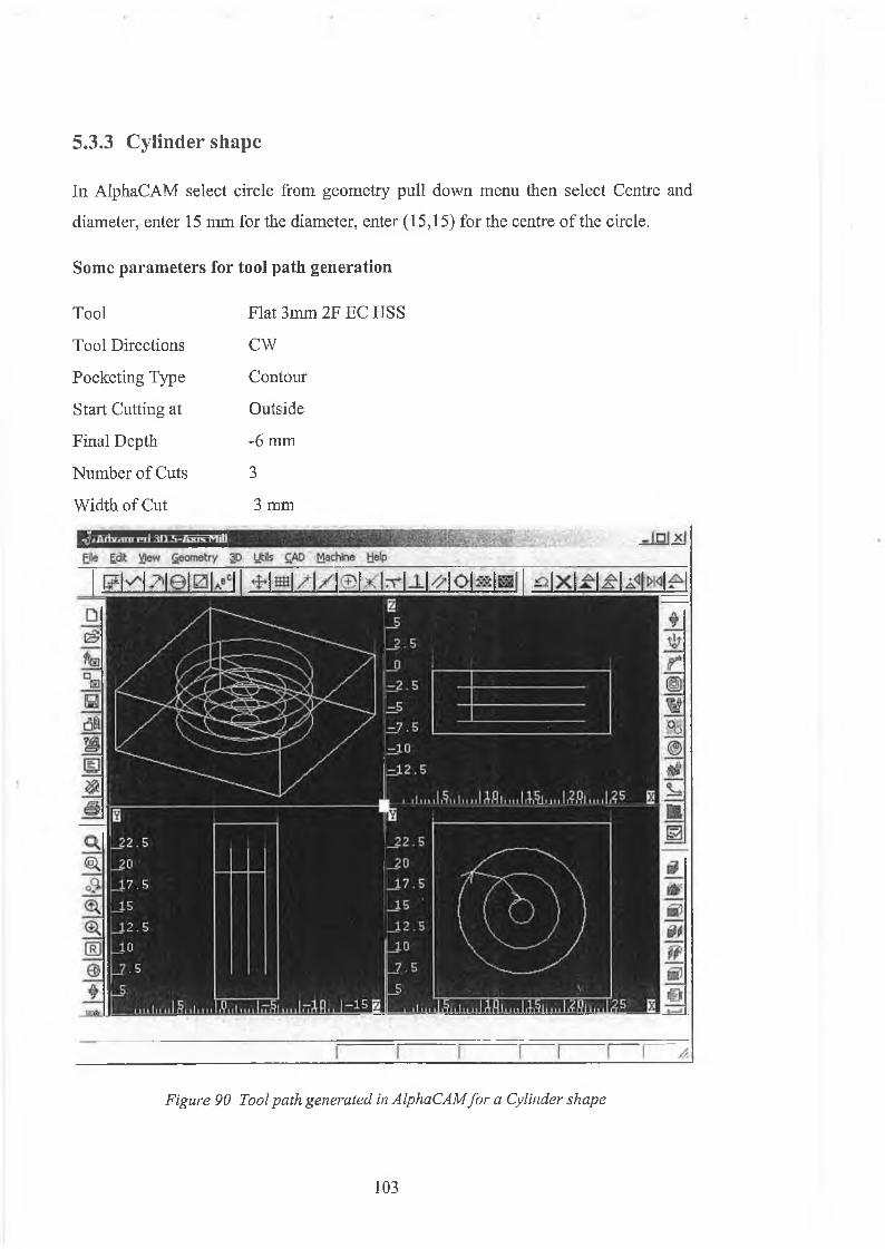
5.3.3 Cylinder shape
In AlphaCAM select circle from geometry pull down menu then select Centre and
diameter, enter 15 mm for the diameter, enter (15,15) for the centre o f the circle.
Some parameters for tool path generation
Figure 90 Tool path generated in AlphaCAM fo r a Cylinder shape
Tool
Tool Directions
Pocketing Type
Start Cutting at
Final Depth
Number o f Cuts
Width of Cut
Flat 3mm 2F EC HSS
CW
Contour
Outside
-6 mm
3
3 mm
103

m <sim m
SI
Figure 91 Cylinder shape deposited using Wax Droplet RP System
104

Select rectangular in AlphaCAM from geometry pull down menu, enter (0,0) for the
First comer and (21,18) for the second comer.
Some parameters for tool path generation
Tool Flat 3 mm 2F EC HSS
Tool Directions CCW
Pocketing Type Linear
Final Depth -6 mm
Number of Cuts 3
Width of Cut 3 mm
5.3.4 Rectangular (21*18) shape
Figure 92 Tool path generated in AlphaCAM for (21 *18) Rectangular shape
-^'Advanced 3D 5-Axis Mill
Elle Edit View g e o m e try 3D Utils £A D M achine ¡Help
105

i i
Figure 93 Rectangular (21 *18) shape deposited using Wax Droplet RP System
106
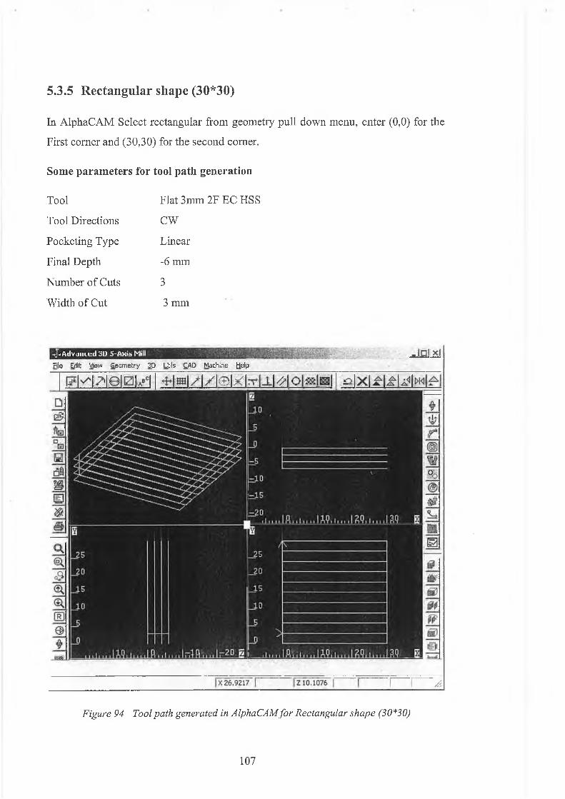
5.3.5 Rectangular shape (30*30)
In AlphaCAM Select rectangular from geometry pull down menu, enter (0,0) for the
First comer and (30,30) for the second comer.
Some parameters for tool path generation
Tool Flat 3mm 2F EC HSS
Tool Directions CW
Pocketing Type Linear
Final Depth -6 mm
Number of Cuts 3
Width of Cut 3 mm
^ Advanced 3D 5-Axis Mill _____File Edit View G eo m e try 3D Utils CAD M achine ¡Help
Figure 94 Tool path generated in AlphaCAMfor Rectangular shape (30*30)
107
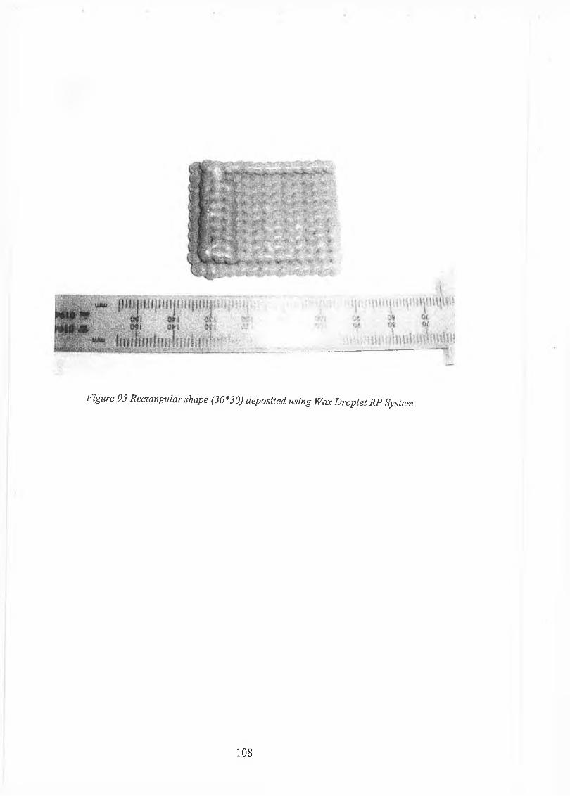
Figure 95 Rectangular shape (30*30) deposited using Wax Droplet RP System
108
Chapter 6 Conclusion and Suggested Future Work
6.1 Advantages of Using CAD/CAM for RP.
Even thought this technique is not fully automated, where the tool path has to be
generated in CAD/CAM software for the design, this may causes a delay in the
operation, but it has many advantages:
a. Data transfer: many problems related to this issue were discussed in section 1.
By directly using CAD/CAM packages the author overcame this problem, and
there is no need to transfer CAD data to any other format.
10. Process planning: such as slicing the geometry, tool path generation and
building the support structure, are the basic requirements for any RP software.
Using this strategy ends the need to develop algorithms to carry out these
tasks.
11. Availability of CAD/CAM: another advantage o f using this strategy is the
availability of CAD/CAM software; the large number of operators and
engineers are familiar with using these software and using CNC code. This
will expand the use o f material addition technology on the horizon.
12. Multi patterns structure: A different filling pattern in the same layer gives a
different surface finish and different material property; this technique is
possible in this strategy by machining different areas with different patterns.
13. Adaptive Slicing technology: is a new technique used to obtain the surface
finish with minimal number of layers see section 2, this technique can be
achieved using the suggested strategy.
14. Multiple material fabricate: Although this is a very new technique RP see
section 2.6.5, the strategy suggested is capable o f performing this task, by
selecting different machining tools in CAD/CAM system for each material
requested, then use its tool path to drive the selected deposition head, which
deposits the specified material.
109
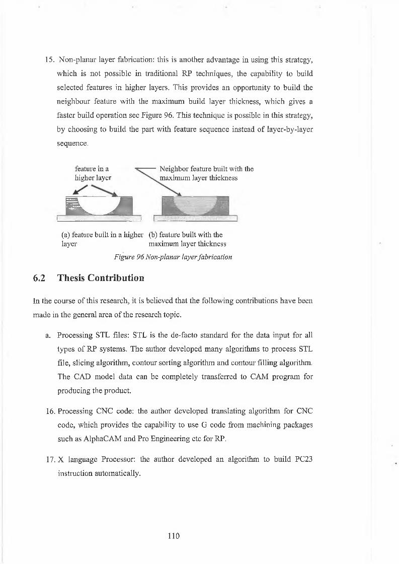
15. Non-planar layer fabrication: this is another advantage in using this strategy,
which is not possible in traditional RP techniques, the capability to build
selected features in higher layers. This provides an opportunity to build the
neighbour feature with the maximum build layer thickness, which gives a
faster build operation see Figure 96. This technique is possible in this strategy,
by choosing to build the part with feature sequence instead of layer-by-layer
sequence.
feature in a — Neighbor feature built with thehigher layer maximum layer thickness
, 1 L . J S l i
(a) feature built in a higher (b) feature built with the layer maximum layer thickness
Figure 96 Non-planar layer fabrication
6.2 Thesis Contribution
In the course of this research, it is believed that the following contributions have been
made in the general area of the research topic.
a. Processing STL files: STL is the de-facto standard for the data input for all
types of RP systems. The author developed many algorithms to process STL
file, slicing algorithm, contour sorting algorithm and contour filling algorithm.
The CAD model data can be completely transferred to CAM program for
producing the product.
16. Processing CNC code: the author developed translating algorithm for CNC
code, which provides the capability to use G code from machining packages
such as AlphaCAM and Pro Engineering etc for RP.
17. X language Processor: the author developed an algorithm to build PC23
instruction automatically.
110
18. Modifying CAM/RP to become user-friendly software to control the Wax
Droplet RP System. CAM/RP can be executed by selecting Export from file
men
6.3 Suggested Future W ork
The wax droplet RP system was designed to deposit the wax as droplets, this system
can be enhanced to deposit the wax as bead similar to FDM system, and also it can be
combined to build a hybrid system.
Although the new strategy proceeds in different steps as emphasized early, and does
not use STL format for data exchange, it is still possible to communicate with the
other RP systems.
A different format called Slice format are used as a data exchange format in some
systems. After the STL data o f the geometry is imported to the system, the slice
format is generated for the part. Slice format stores the geometrical information for
each layer. This information includes the layer thickness the boundaries of the solid
material, the hatches, which define the filling and the support structures. Slice format
has been considered as a replacement for STL format [5].
Developing an algorithm to extract the required information for each layer from CNC
code then format it into one of the slicing format interfaces such as CLI, LEAF, HP-
GL, and SLC format. This information can be feed to any commercial RP machine
that uses this format.
I l l
References
1. Gan G.K. Jacob, Chua Chee and Tong Mei, “Development o f a new rapid
prototyping interface”, Computers in Industry, Elsevier Science, Vol: 39, Issue 1,
June 1999, Pages 61-70, PII: S0166-3615(98)00124-9.
2. Carl Machover, “The CAD/CAM Hand book”, The McGraw-Hill Companies, Inc.
1996
3. D.T.Pham and R.S. Gault, “A comparison of rapid prototyping technologies”,
International Journal of Machine Tools and Manufacture ,Vol 38, Issues 10-11
1998 Pages 1257-1287 PII: S0890-6955(97)00137-5.
4. C. J. Luisa, J. Vivancosb, I. Puertas, L. Costab and M. A. Sebastianc,
“Comparative analysis of injection systems for manufacturing parts”, Journal of
Materials Processing Technology, Elsevier Science, Volumes 143-144, 20
December 2003, Pages 112-117, doi:10.1016/S0924-0136(03)00330-3,.
5. Vinod Kumar and Debasish Dutta, “An assessment o f data formats for layered
manufacturing”, Advances in Engineering Software, Vol: 28, Issue 3,April 1997,
Pages 151-164, PII: S0965-9978(96)00050-6.
6. Xue Yan & P Gu, “A review of rapid prototyping technologies and systems”,
Computer-Aided Design, Elsevier Science, Vol: 28,No.4, 1996, pp.307-318.
7. http://www.warwick.ac.uk/atc/rpt/Techniques/cad.htm.
8. Y.H Chen and C.T. Ng, “Integraed Revers Engineering and prototyping”,
Computers & Industrial Engineering, Published by Elsevier, Vol: 33, Issues 3-4
1997, pp.481-484, doi:10.1016/S0360-8352(97)00173-3.
9. S.H. Choi and K.T. Kwok, “Hierarchiacal slice contours for layered-
manufacturing”, Computers in Industry, Elsevier Science, Volume 48, Issue 3,
August 2002, Pages 219-239, PII: S0166-3615(02)00040-4.
112

10. Sang C. Park, and Yun C. Chung, “Tool-path generation from measured data”,
Computer-Aided Design, Elsevier Science, Volume 35, Issue 5 , 15 April 2003,
Pages 467-475, doi:10.1016/S0010-4485(02)00070-2.
11. Y. F. Wu, Y. S. Wong, H. T. Loh and Y. F. Zhang, “Modelling cloud data using
an adaptive slicing approach”, Computer-Aided Design, Elsevier Science, Volume
36, Issue 3, March 2004, Pages 231-240, doi: 10.1016/S0010-4485 (03) 00097-6.
12 .1. Stroud and P.C. Xirouchakis, “STL and extensions”, Advances in Engineering
Software, Elsevier Science, Vol 31, Issue 2, February 2000, Pages 83-95, PII:
S0965-9978 (99) 00046-0.
13. http://www.uclan.ac.uk/clt/calm/stl.htm
14. F,. Loh, H.T. Wong, Y. S, Xu, “Considerations and election of optimal orientation
for different rapid prototyping sytems”. Rapid Prototyping Journal, Elsevier,
Volume 5, Issue 2, 1999, Pages 54-60.
15. H. T. Loh, Y. F. Wu, Y. S. Wong and Y. F. Zhang, “Modelling and optimisation
o f Rapid Prototyping”, Computers in Industry, Elsevier, Volume 47, Issue 1,
January 2002, Pages 39-53, PII: S0166-3615(01)00140-3.
16. Sung-Min Hur, Kyung-Hyun Choi, Seok-Hee Lee, and Pok-Keun Chang,
“Determination of fabricating orientation and packing in SLS process”, Journal of
Materials Processing Technology, Elsevier., Volume 112, Issues 2-3 , 25 May
2001, Pages 236-243, doi:10.1016/S0924-0136(01)00581-7.
17. Weiyin Ma and Peiren He, “An adaptive slicing and selective hatching strategy for
layered manufacturing”, Journal of Materials Processing Technology, Elsevier,
Volumes 89-90, 19th May 1999, Pages 191-197, PII: S0924-0136(99)00043-6.
18. K.P Karunakam, P. Vivekananda Shanmuganathan, Sanjay Janardhan Jadhav,
Prashabt Bhadaura, Ashish Pandey, “Rapid prototyping of metallic parts and
moulds”, Journal o f Materials Processing Technology, Elsevier, Volume 105,
Issue 3, 29 September 2000, Pages 371-381, PII: S0924-0136(00)00586-0.
19. You-Min Huang, , Jeng-Ywen Jeng and Cho-Pei Jiang, “Increased accuracy by
using dynamic finite element method in the constrain-surface stereolithography
113

system”, Journal of Materials Processing Technology, Volume 140, Issues 1-3 ,
22nd September 2003, Pages 191-196, Proceedings o f the 6th Asia Pacific
Conference on Materials Processing, Elsevier, doi:10.1016/S0924-
0136(03)00711-8.
20. P. Kulkami, D. Dutta, “Deposition strategies and resulting part stiffnesses in fused
deposition modeling”, Journal o f Manufacturing Science and Engineering,
Transactions o f the ASME , Elsevier, Volume 121, Issue 1, February 1999, Pages
93-103.
21. R. E. Williams, S. N. Komaragiri, V.L. Melton and R.R. Bishu, “Investigation of
the effect o f various build methods on the performance o f rapid prototyping
(stereolithography)”, Journal of Materials Processing Technology, Volume 61,
Issues 1-2, August 1996, Pages 173-178
22. http://www.bath.ac.uk
23. J. C. Ferreira, a and A. Mateusb, “A numerical and experimental study of fracture
in RP stereolithography patterns and ceramic shells for investment casting”,
Journal o f Materials Processing Technology, Elsevier, Volume 134, Issue 1, 1
March 2003, Pages 135-144, doi:10.1016/S0924-0136(02)01034-8.
24. 3D system annual report 2001, http://www.ien.it/ar01/ar/is.html.
25. Liu Hongjun, Fan Zitian, Huang Naiyu and Dong Xuanpu, “A note on rapid
manufacturing process of metallic parts based on SLS plastic prototype”, Journal
of Materials Processing Technology, Elsevier, Volume 142, Issue 3 , 10 December
2003, Pages 710-713, doi:10.1016/S0924-0136(03)00811-2.
26. http://home.att.net
27. Y. S. Liao, L. C. Chiu and Y. Y. Chiu, “A new approach o f online waste removal
process for laminated object manufacturing (LOM)”, Journal of Materials
Processing Technology, Elsevier, Volume 140, Issues 1-3 , 22 September 2003,
Pages 136-140, Proceedings of the 6th Asia Pacific Conference on Materials
Processing, doi:10.1016/S0924-0136(03)00690-3.
114
28. Bernhard Mueller and Detlef Kochan, “Laminated object manufacturing for rapid
tooling and pattemmaking in foundry industry”, Computers in Industry, Volume
39, Issue 1, June 1999, Pages 47-53
29. http://www.zcorp.com/
30. Suwat Jirathearanat, Victor Vazquez, Ciro A. Rodrigues and Taylan Altan
“Virtual processing - application o f rapid prototyping for visualisation of metal
forming processes”, Journal of Materials Processing Technology, Elsevier, Vol:
98, Issue 1,15 January 2000, Pages 116-124 PH: S0924-0136(99)00312-X
31. http://www.stratasys.com/
32. K.Y, Peshges, “Comparative analysis o f SL and FDM methods”, Elsevier, July
1999, Pages 34-38.
33. D etlf Kochan, Chua Chee Kai, and Du Zhaohui, “Rapid prototyping issues in the
21st Centry”, Computers in Industry, Elsevier, Volume 39, Issue 1, June 1999,
Pages 3-10, PH: S0166-3615(98)00125-0.
34. Jack G. Zhou, Daniel Herscovici and Calvin C. Chen, “Parametric process
optimization to improve the accuracy of rapid prototyped stereolithography parts”,
International Journal o f Machine Tools and Manufacture, Volume 40, Issue 3,
February 2000, Pages 363-379.
35. Hong-Tzong Yau, Chuan-Chu Kuo and Chih-Hsiung Yeh, “Extension o f surface
reconstruction algorithm to the global stitching and repairing of STL models”,
Computer-Aided Design, Elsevier, Volume 35, Issue 5 , 15 April 2003, Pages
477-486, doi: 10.1016/S0010-4485(02)00078-7
36. S. H. Masood, W. Rattanawong and P. Iovenitti, “A generic algorithm for a best
part orientation system for complex parts in rapid prototyping”, Journal of
Materials Processing Technology, Elsevier, Volume 139, Issues 1-3 , 20 August
2003, Pages 110-116, doi:10.1016/S0924-0136(03)00190-0.
37. “Software Solutions for Rapid Prototyping” Ian Gibson, Professional Engineering
Publ; August, 2002; ISBN: 1860583601.
115

38. Pulak M. Pandey, N. Venkata Reddy, and Sanjay G. Dhande, “Improvement of
surface finish by staircase machining in fused deposition modeling”, Journal of
Materials Processing Technology, Elsevier, Volume 132, Issues 1-3, 10th January
2003, Pages 323-331, doi:10.1016/S0924-0136(02)00953-6.
39. H. T. Loh, Y. F. Zhang, Y. F. Wu and Y. S. Wong, “An adaptive slicing approach
to modelling cloud data for rapid prototyping”, Journal o f Materials Processing
Technology, Elsevier, Volume 140, Issues 1-3, 22 September 2003, Pages 105-
109, doi: 10.1016/S0924-0136(03)00824-0.
40. P. M. Pandey, N. V. Reddy, and S. G. Dhande 1, “Real time adaptive slicing for
fused deposition modelling”, International Journal of Machine Tools and
Manufacture, Elsevier, Volume 43, Issue 1 , January 2003, Pages 61-71,
doi:10.1016/S0890-6955(02)00164-5
41. Wenbin Hong, Yong Tsui Lee, and Haiqing Gong, “Thermal analysis of layer
formation in a stepless rapid prototyping process”, Applied Thermal Engineering,
Elsevier August 2003.
42. Y. Tanga, H. T. Loha, Y. S. Wongb, J. Y. H. Fuh, b, L. Lub and X. Wangb,
“Direct laser sintering of a copper-based alloy for creating three-dimensional
metal parts”, Journal o f Materials Processing Technology, Elsevier, Volume 140,
Issues 1-3 , 22nd September 2003, Pages 368-372, Proceedings of the 6th Asia
Pacific Conference on Materials Processing, doi:10.1016/S0924-0136(03)00766-
0.
43. M. W. Khainga, J. Y. H. Fuh, b and L. Lub, “Direct metal laser sintering for rapid
tooling: processing and characterisation of EOS parts”, Journal of Materials
Processing Technology, Elsevier, Volume 113, Issues 1-3, 15th June 2001, Pages
269-272, doi:10.1016/S0924-0136(01)00584-2.
44. Doo-Sun Choi, S. H. Leeb, B. S. Shina, K. H. Whanga, Y. A. Songc, S. H. Parke
and H. S. Jeed, “Development of a direct metal freeform fabrication technique
using C 02 laser welding and milling technology”, Journal of Materials
Processing Technology, Elsevier, Volume 113, Issues 1-3 , 15th June 2001, Pages
273-279, doi: 10.1016/S0924-0136(01 )00652-5.
116
45. http://www.me.psu.edu
46. W. K. Chiu and S. T. Tan, “Multiple material objects from CAD representation to
data format for rapid prototyping”, Computer-Aided Design, Elsevier Volume 32,
Issue 12 , October 2000, Pages 707-717, doi:10,1016/S0010-4485(00)00046-4.
47. Arthur L. Foston, Carolena L. Smith and Tony Au, “Fundamentals o f Computer-
Integrated Manufacturing”, Prentice-Hall Inc 1991.
48. C. Ray Asfahl, “Robots and manufacturing automation”, John Wiley & Sons
1992.
49. M. Lynch, “Computer Numerical control for Machining”, McGraw-Hill, 1992,
ISBN: 0070392234.
50. Dr. Tamas Szecsi, “Smart autonomous Machine tools and equipment”, January
2001.
51. http://www.wokingham.demon.co.Uk/prog/programming.htm#G-Codes.
52. Dr. Tang Sai Hong, “Rapid prototyping using precision robotic manipulator”,
fulfilment for degree of Doctor of Philosophy, DCU September 2000.
53. Ibrahim, M Eng, “ Computer application-electro mechanical systems”, fulfilment
for degree of Masters o f Engineering, DCU February 2004.
54. PC23 indexer User Guide Compumotor Division Parker Hannifin Corporation
P/n 88-007015-03E.
55. Mark F. Russo, Martin M. Echols, “Automating Science and Engineering
Laboratories with Vsual Basic”, John Wiley & Sons, 1999, ISBN: 0471254932.
56. Bruce Stirling, “Micro-blob deposition of wax as a prototype technology”, final
year project report, School of mechanical and manufacturing engineering, DCU,
2000 .
57. Jeffrey H Kingston, “Algorithms and Data Structures”, Addison Wesley Longman
Limited, ISBN 0-201-40374-9,1997, P 221
117

58. Julia Case Bradly, Anita C. Millspaugh, “Programming in Visual Basic 6.0”
McGraw-Hill Higher Education, 2002,ISBN 0-07-251381-0.
59. Theo Pavlidis, “Algorithms for Graphics and Image Processing”, computer
Science press, 1976, ISBN 0-914894-65-X.
60. Richard Stretton, “Fanuci.s.o. Programming notes”, chapter 2, Cincinnati Machine
(UK)
118

Appendix A Preparatory codes [59]
G code Function Modal Group
GO Linear Rapid
Yes 01Gl Linear Feed
G2 Circular clockwies Feed
G3 Circular Anti-clockwies Feed
G4 Dwell No 00
G7.1 Cylindrical Interpolation Yes 00
G9 Exact Stop No 00
G10 Programmable Data No 00
G il Programmable Data cancel No 00
G15 Polar Coordinate cancelYes 17
G16 Polar Coordinate
G17 XY Plane selection
Yes 02G18 XZ Plane selection
G19 YZ Plane selection
G20 Inch unitsYes 06
G21 Metric units
G27 Reference position return
checkNo
00
G28 Returen to Reference
position
119

G29 Returen from Reference
position
G30 2nd ,3rd & 4th Reference
position Returen
G31 Skip Function No 00
G40 Cutter Compensation Cancel
G41 Cutter Compensation Left Yes 07
G42 Cutter Compensation Rigth
G43 Tool length Compensation+
G44 Tool length Compensation-Yes 08
G49 Tool length Compensation
cancel
G50 Scaling CancelYes 11
G51 Scaling Active
G52 Local coordinate System Yes
G53 Machine Coordinate System
G54 Workpice Coordinate System
114
G55 Workpice Coordinate System
G56 2
Workpice Coordinate System
3
G57 Workpice Coordinate System
4
120
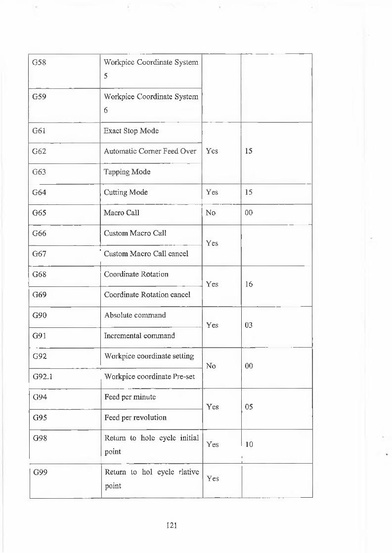
G58 Workpice Coordinate System
5
G59 Workpice Coordinate System
6
G61 Exact Stop Mode
Yes 15G62 Automatic Comer Feed Over
G63 Tapping Mode
G64 Cutting Mode Yes 15
G65 Macro Call No 00
G66 Custom Macro CallYes
G67 Custom Macro Call cancel
G68 Coordinate RotationYes 16
G69 Coordinate Rotation cancel
G90 Absolute commandYes 03
G91 Incremental command
G92 Workpice coordinate settingNo 00
G92.1 Workpice coordinate Pre-set
G94 Feed per minuteYes 05
G95 Feed per revolution
G98 Return to hole cycle initial
pointYes 10
G99 Return to hoi cycle rlative
pointYes
121
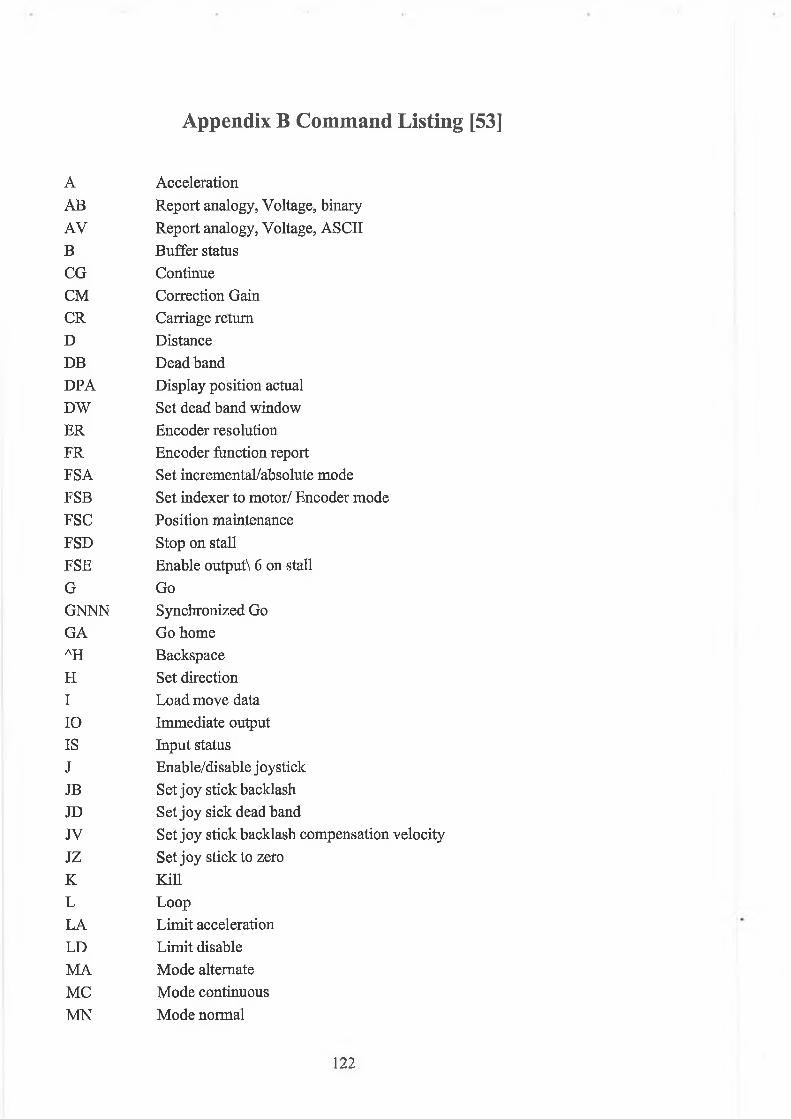
Appendix B Command Listing [53]
A AccelerationAB Report analogy, Voltage, binaryAY Report analogy, Voltage, ASCIIB Buffer statusCG ContinueCM Correction GainCR Carriage returnD DistanceDB Dead bandDPA Display position actualDW Set dead band windowER Encoder resolutionFR Encoder function reportFSA Set incremental/absolute modeFSB Set indexer to motor/ Encoder modeFSC Position maintenanceFSD Stop on stallFSE Enable output\ 6 on stallG GoGNNN Synchronized GoGA Go homeAH BackspaceH Set directionI Load move dataIO Immediate outputIS Input statusJ Enable/disable joystickJB Set joy stick backlashJD Set joy sick dead bandJV Set joy stick backlash compensation velocityJZ Set j oy stick to zeroK KillL LoopLA Limit accelerationLD Limit disableMA Mode alternateMC Mode continuousMN Mode normal
122
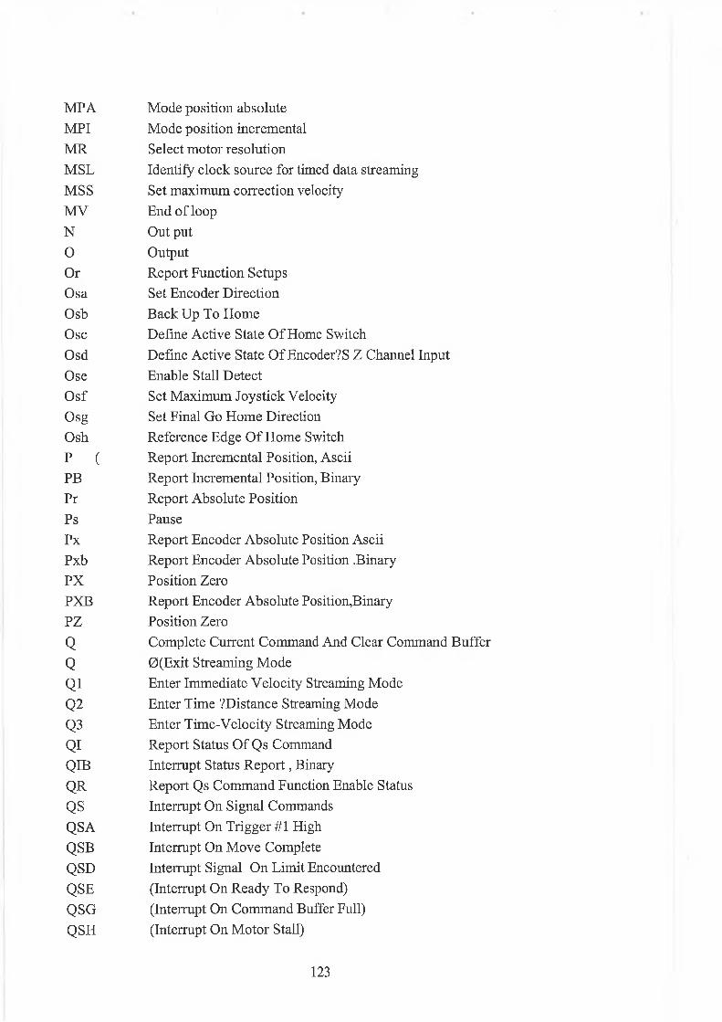
MPA Mode position absoluteMPI Mode position incrementalMR Select motor resolutionMSL Identify clock source for timed data streamingMSS Set maximum correction velocityMV End of loopN Out put0 OutputOr Report Function SetupsOsa Set Encoder DirectionOsb Back Up To HomeOsc Define Active State O f Home SwitchOsd Define Active State O f Encoder? S Z Channel InputOse Enable Stall DetectO sf Set Maximum Joystick VelocityOsg Set Final Go Home DirectionOsh Reference Edge O f Home Switch
P ( Report Incremental Position, AsciiPB Report Incremental Position, BinaryPr Report Absolute PositionPs PausePx Report Encoder Absolute Position AsciiPxb Report Encoder Absolute Position .BinaryPX Position ZeroPXB Report Encoder Absolute Position,BinaryPZ Position Zero
Q Complete Current Command And Clear Command Buffer
Q 0(Exit Streaming Mode
Q1 Enter Immediate Velocity Streaming ModeQ2 Enter Time ?Distance Streaming Mode
Q3 Enter Time-Velocity Streaming Mode
QI Report Status O f Qs CommandQIB Interrupt Status R eport, BinaryQR Report Qs Command Function Enable StatusQS Interrupt On Signal CommandsQSA Interrupt On Trigger #1 HighQSB Interrupt On Move CompleteQSD Interrupt Signal On Limit EncounteredQSE (Interrupt On Ready To Respond)QSG (Interrupt On Command Buffer Full)QSH (Interrupt On Motor Stall)
123
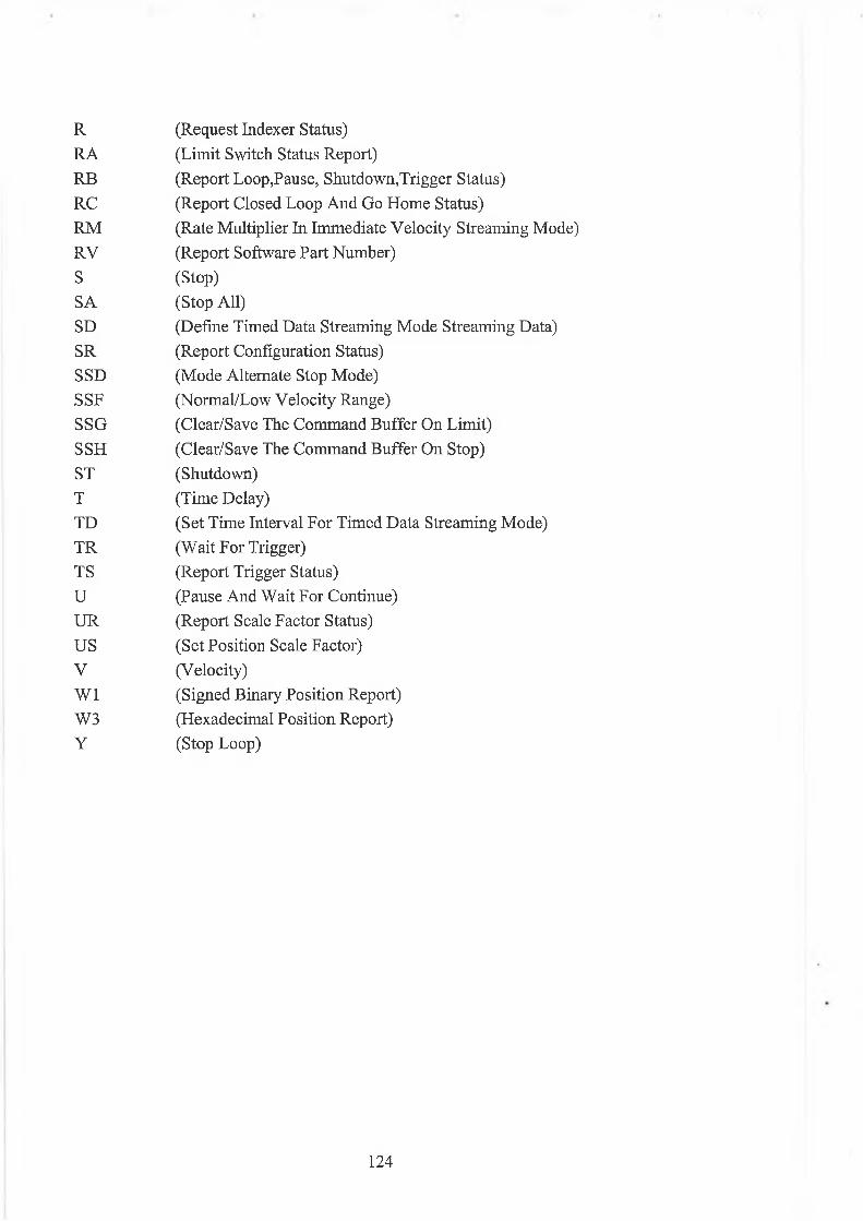
R (Request Indexer Status)RA (Limit Switch Status Report)RB (Report Loop,Pause, Shutdown,Trigger Status)RC (Report Closed Loop And Go Home Status)RM (Rate Multiplier In Immediate Velocity Streaming Mode)RV (Report Software Part Number)S (Stop)SA (Stop All)SD (Define Timed Data Streaming Mode Streaming Data)SR (Report Configuration Status)SSD (Mode Alternate Stop Mode)SSF (Normal/Low Velocity Range)SSG (Clear/Save The Command Buffer On Limit)SSH (Clear/Save The Command Buffer On Stop)ST (Shutdown)T (Time Delay)TD (Set Time Interval For Timed Data Streaming Mode)TR (Wait For Trigger)TS (Report Trigger Status)U (Pause And Wait For Continue)U R (Report Scale Factor Status)US (Set Position Scale Factor)V (Velocity)W1 (Signed Binary Position Report)W3 (Hexadecimal Position Report)Y (Stop Loop)
124
AppendixC CAD/RP
Appendix C 1: X-Y menu algorithm
Picture l.ClsOpen "C:\triangles.txt" For Input As #1 Open "C:\Drawing.txt" For Output As #2 Do Until EOF(l)Input #1, xa, ya, za, xb, yb, zb, xc, yc, zcWrite #2, xa, ya, xb, ybWrite #2, xa, ya, xc, ycWrite #2, xc, yc, xb, ybLoopClose #1Close #2mnuzoom Click
Appendix C 2: 3D menu
Open "C:\triangles.txt" For Input As #1 Open "C:\Drawing.txt" For Output As #2 Picture l.Cls Do Until EOF(l)Input #1, xa, ya, za, xb, yb, zb, xc, yc, zc la = Sqr(xa A 2 + ya A 2) ta = atan2(xa, ya)xa = la * Cos((30 + ta) * 3.14 / 180) ya = za + la * Sin(30 * 4.14 /180) lb = Sqr(xb A 2 + yb A 2) tb = atan2(xb, yb)xb = lb * Cos((30 + tb) * 3.14 /180) yb = zb + lb * Sin(30 * 4.14 / 180)Lc = Sqr(xc A 2 + yc A 2) tc = atan2(xc, yc)xc = Lc * Cos((30 + tc) * 3.14 /180) yc = zc + Lc * Sin(30 * 4.14 / 180)Write #2, xa, ya, xb, yb Write #2, xa, ya, xc, yc Write #2, xc, yc, xb, yb
125
Loop Close #1 Close #2 mnuzoom Click
Appendix C3: Slicing algorithmt iji iji i|C iji iji iji iji iji iji ^ ^ iji •}* ^ ^ 'I' ^ 'I' •J’ 'f' iji 4? iji f|< iji iji >{t /{i p{« iji 5|i iji »(• lji iji rj* ij* ¡|i iji rjC ¡ji -j* iji t|i iji t|i t
starting slicing with layer thickness of d1 iji iji iji iji iji ifi iji iji if! ijc iji iji iji iji iji iji iji r|i iji iji ifi if. iji iji iji iji i|i i|i iji iji iji iji iji iji iji iji rji iji iji iji iji iji iji iji iji iji iji iji iji iji iji iji iji iji iji iji iji ifi iji iji iji iji iji iji iji
Public Sub SliceSTL() outfilel = "c:\slidesSTL.TXT" n = 0Call Picturel.Cls Open outfilel For Output As #2 Open infile For Input As #1 Do Until EOF(l)
Input #1, Target I f Target = "outer loop" Then
Input #1, Target 1 Vertex (Target 1) x l = Val(Vertex_x) y l = Val(Vertex_y) z l = Val(Vertex_z)
Input #1, Target2 Vertex (Target2) x2 = Val(Vertex_x) y l = Val(Vertex_y) z2 = Val(Vertex_z)
Input #1, Target3 Vertex (Target3) x3 = Val(Vertex_x) y3 = Val(Vertex_y) z3 = Val(Vertex_z)
' check which line intersect with the plane & find the intersection points
If z = z l And z = z2 And z = z3 Then ignor = 1
126
Elself z = z l And z = z2 And z3 > z Then ' Groub 4 Case a Write #2, x l , y l , x2, y2 Picturel.Line (x l, yl)-(x2, y2)Call slow DoEvents n = n + 1Elself z = z l And z = z3 And z2 > z Then ' Groub 4 Case b Write #2, x l, y l, x3, y3 Picturel.Line (x l, yl)-(x3, y3)Call slow DoEvents n = n + 1Elself z = z2 And z = z3 And zl > z Then 1 Groub 4 Case c Write #2, x2, y2, x3, y3 Picture 1 .Line (x2, y2)-(x3, y3)Call slow DoEvents n = n + 1
Elself z = z l And ((z > z2 And z < z3) Or (z < z2 And z > z3)) Then 'Groub 2 Case a x23 = x2 + (z - z2) * (x3 - x2) / (z3 - z2) y23 = y2 + (z - z2) * (y3 - y2) / (z3 - z2)Write #2, x l, y l, x23, y23 Picturel.Line (x l, yl)-(x23, y23)Call slow DoEvents n = n + 1
Elself z = z2 And ((z > zl And z < z 3 ) O r ( z < z l And z > z3)) Then ’Groub 2 Case b x l3 = x l + (z - z l) * (x3 - x l) / (z3 - z l) y 13 = y l + ( z - z l ) * (y3 - y l) / ( z 3 - z l)Write #2, x2, y2, x l3 , y 13 Picturel.Line (x2, y2)-(xl3, y 13)Call slow DoEvents n = n + 1
Elself z = z3 And ((z > z 1 And z < z2) Or (z < zl And z > z2)) Then 'Groub 2 Case c x l2 = xl + (z - z l) * (x2 - x l) / (z2 - z l) y 12 = yl + (z - z l) * (y2 - y l) / (z2 - z l)Write #2, x3, y3, x l2 , y 12
127
Picture 1.Line (x3, y3)-(xl2, y l2)Call slow DoEvents n = n + 1
Elself (z > z l And z < z2) Or (z < zl And z > z2) Then x l2 = x l + (z - z l) * (x2 - x l) / (z2 - z l) y 12 = y l + (z - z l) * (y2 - y l) / (z2 - z l)
If (z > zl And z < z3) Or (z < zl And z > z3) Then 'Group 1 case A x l3 = x l + (z - z l) * (x3 - x l) / (z3 - z l) y 13 = yl + (z - z l) * (y3 - y l) / (z3 - z l)Write #2, x l2 , y l2 ,x l3 ,y l3 Picture 1.Line (xl2 , y l2)-(xI3, y 13)
Call slow DoEvents n = n + 1
Elself (z > z2 And z < z3) Or (z < z2 And z > z3) Then 'Group 1 case B x23 = x2 + (z - z2) * (x3 - x2) / (z3 - z2) y23 = y2 + (z - z2) * (y3 - y2) / (z3 - z2)Write #2, x l2 , y l2 , x23, y23 Picture 1.Line (x l2 , yl2)-(x23, y23)
Call slow DoEvents n = n + 1 End If
Elself (z > z3 And z < z2) Or (z < z3 And z > z2) Then ' Group 1 Case C x23 = x2 + (z - z2) * (x3 - x2) / (z3 - z2) y23 = y2 + (z - z2) * (y3 - y2) / (z3 - z2)
If (z > zl And z < z3) Or (z < zl And z > z3) Then x l3 = xl + (z - z l) * (x3 - x l) / (z3 - z l) y 13 = yl + (z - z l) * (y3 - y l) / (z3 - zl)Write #2, x23, y23, x l3 , y 13 Picturel.Line (x23, y23)-(xl3, y 13)
Call slow DoEvents n = n + 1 End If
128
End If
End If
Loop Close #1 Close #2 End Sub
Appendix C4 Contour Construction algorithm
Public Sub contour_ordering() coun_con = 0 Call Picturel.Clsoutfile2 = "c:\countor_in _order.TXT"Open outfilel For Input As #1 Input #1, xa l, yal, xbl, ybl Close #1Open outfile2 For Output As #2 Write #2, xa l, yal, xbl, y b l, z Close #2Write #6, xa 1, ya 1, xb 1, yb 1, z coun_con = coun_con + 1 Picture 1 .Line (xal, yal)-(xbl, ybl), vbRed For q = 1 To n
If q o 1 ThenOpen outfilel For Input As #1For h = 1 To n 'to pick new line from new contour Input #1, xal, y a l, xb l, ybl rep = 0Open outfile2 For Input As #2 'check if this contour does exist in the new list
Do Until EOF(2)Input #2, a, b, c, e, fIf (xal = a And yal = b And xbl = c And ybl = e ) Or (xal = c And yal = e
And xbl = a And ybl = b) Then rep = rep + 1 End If Loop
Close #2
129
If rep = 0 Then Exit For End If
Next h Close #1
Open outfile2 For Append As #2 'add this line to new listWrite #2, x a l, y a l, xb l, ybl, z Close #2Write #6, x a l, ya l, xb l, ybl, z conn_con = coun_con + 1 Picturel.Line (xal, yal)-(xbl, yb l), vbRed End If
xa = xal ya = yalDo Until xa = xb And ya = yb 1 search to close the contourOpen outfilel For Input As #1For k = 1 To nInput #1, xa2, ya2, xb2, yb2If xbl = xa2 And ybl = ya2 And (xal o xb2 Or yal o yb2) Then Open outfile2 For Append As #2 Write #2, xa2, ya2, xb2, yb2, z Close #2Write #6, xa2, ya2, xb2, yb2, zPicturel.Line (xa2, ya2)-(xb2, yb2), vbRedxal = xa2yal = ya2xb 1 = xb2ybl = yb2xb = xb2yb = yb2coun_con = coun_con + 1Elself xbl = xb2 And ybl = yb2 And (xal o xa2 Or yal o ya2) Then Open outfi!e2 For Append As #2 Write #2, xb2, yb2, xa2, ya2, z Close #2Write #6, xb2, yb2, xa2, ya2, z Picturel.Line (xb2, yb2)-(xa2, ya2), vbRed x a l = xb2 y a1 = yb2 xbl = xa2
130

y b l = ya2 xb = xa2 yb = ya2coun_con= co u n co n + 1End IfDoEventsNext kClose #1DoEventsLoopCall slowIf coun_con >= n ThenExit ForEnd IfNext qClose #1Close #2End Sub
Appendix C5 Filling the pattern algorithm
Public Sub Fill_patren()
| ^ ji* ^ jjj j|# jjj jj* ¡¿j jj* jjj j|# «1# jj* jj# jJj jj; jjj t|* jJ ^ ¡j* j|£ ¡Jj jJ# jpj »J# jjj
' finde intersection with y
outfile4 = "c:\jghdfoiu.txt"Open outfile4 For Output As #15
m = 0For y = (ymin + dyf) To (ymax - dyf) Step dyf
Open outfilel For Input As #4 p = 0 'number o f intersection
For k = 1 To n
Input #4, xa, ya, xb, yb
131

If (y >= ya And y < yb) Or (y >= yb And y < ya) Then p = p + 1x(p )= (y - ya) * (xb - xa) / (yb - ya) + xa End If
Next
Close #4
If p > 0 Then m = m + p For h = 1 To p
Write #15, x(h), y, p Next h End If
DoEvents NextClose #15
' find the pointes in the same livel and joine 1 to 2 and 3 to 4
infile4 = outfile4 Call slowOpen infile4 For Input As #7 k = 1 p = l v = 1 w = 1 n_o_i = 0
For k = 1 To mI Hc 9{î s}« * î|» # * i'fi H: tfî # * sfc # * # * * H« * * & * * * 'A' * # * * H* # # &
'order the points in ths saine level
n_o_i = n_o_i + 1
r = 1Input #7, xa, ya, p x(r) = xa
132

For r = 2 To p Input #7, xa, ya, p x(r) = xa
N ex tr
For v = 1 To (p - 1)I f x(v + 1) < x(v) Then a = x(v) x(v) = x(v + 1 ) x(v + 1) = a
I f v >= 2 Then w = 1For w = v To 1 Step -1 If x(w) < x(w -1 ) Then
b = x(w - 1) x(w -1 ) = x(w) x(w) = b Else Exit For End If
Next w End If
End If Next v
If (-1) A n_o_i < 0 Then
For 1 = 1 To p Step 2
Picture 1.Line (x(l), ya)-(x(l + 1), ya), vbRed Write #6, x(l), ya, x(l + 1), ya, z
Call slow DoEvents
Next 1 Else
For 1 = (p - 1) To 1 Step -2
133
Picture 1.Line (x(l + 1), ya)-(x(l), ya), vbRed Write #6, x(l + 1), ya, x(l), ya, z
Call slow DoEvents
Next 1 End If
k = k + p - 1 DoEvents
Next k Close #7
End Sub
Appendix C6 Simulate the deposition algorithm
Public Sub simulat()x l = 0y l = 0zl = 0D d r o p =3LD = 3
Open outfile5 For Input As #1
Do Until EOF(l)
Input #1, xa, ya, xb, yb, zl
Dx = xb - xa dy = yb - yaDt = (Dx A 2 + dy A 2) A (1 / 2)
If Abs(Dt) >= LD Then
134
ran = Dt / LD 'number o f motionwx = xa wy = yaFor k = 1 To mn
If Dx = 0 And dy o 0 Then wy = wy + LD * dy / Dt
Elself Dx <> 0 And dy = 0 Then wx = wx + LD * Dx / Dt
E lself dy o 0 And Dx o 0 Then wx = wx + LD * Dx / Dt wy = wy + LD * dy / Dt End IfPicture 1.Circle (wx, wy), D_drop / 2 \ Deposition_colorCall slowDoEvents
Write #5, wx, wy, zl
Call slow
Next k
End If
Loop
Close #1
End Sub
Appendix C7 Build the instruction file
Public Sub Build() x l = 0 y l = 0
List 1 .ClearList 1. Visible = True
135
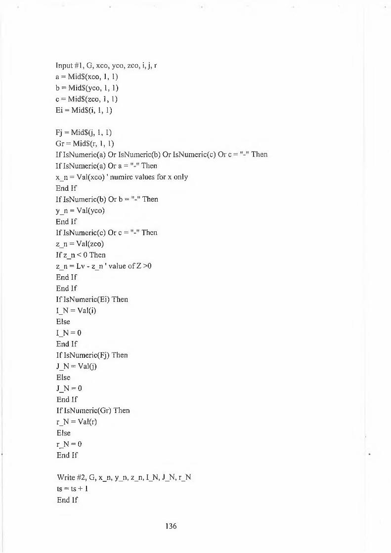
Input #1, G, xeo, yco, zco, i, j, r a = Mid$(xco, 1,1) b = Mid$(yco, 1,1) c = Mid$(zco, 1,1)Ei = Mid$(i, 1, 1)
Fj = Mid$(j, 1,1)Gr = Mid$(r, 1, 1)If IsNumeric(a) Or IsNumeric(b) Or IsNumeric(c) Or c = ThenI f IsNumeric(a) Or a = Thenx_n = V al(xeo)1 numirc values for x onlyEnd IfIf IsNumeric(b) Or b = Then y_n = Val(yeo)End IfIf IsNumeric(e) Or c = Then z_n = Val(zco)If z_n < 0 Thenz_n = Lv - z_n ' value of Z >0End IfEnd IfIf IsNumeric(Ei) Then I_N = Val(i)Else I_N = 0 End IfIf IsNumeric(Fj) Then J_N = Val(j)Else J_N = 0 End IfIf IsNumeric(Gr) Then r_N = Val(r)Else r_N = 0 End If
Write #2, G, x_n, y_n, z_n, I_N, J_N, r_N ts = ts + 1 End If
136

End IfVx = Format$(Vx, "0.0000")Vy = Format$(Vy, "0.0000")First_part = " LD3" & Positionm odes & M odem oves & xaxis_motor & "V" &
Vx & xaxis motor & "D" & Dxpsecond_part = yaxism otor & "V" & Vy & yaxism otor & "D" & Dyp & " G 12
P "End If
result = First_part & second_partWrite #2, resultWrite #2, message 1Write #2, message2Listl.Addltem resultListLAddltem message 1Listl.Addltem message2x l = x2y l = y 2LoopClose #2Close #1End Sub
137
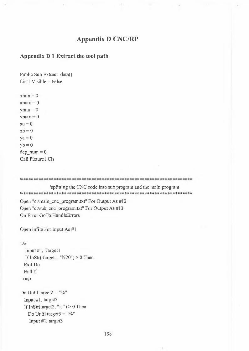
Appendix D CNC/RP
Appendix D 1 Extract the tool path
Public Sub Extract_data()List 1. Visible = False
xniin = 0 xmax = 0 ymin = 0 ymax — 0 xa = 0 xb = 0 ya = 0 yb = 0dep_num = 0 Call Picturel.Cls
'splitting the CNC code into sub program and the main programI $ $ & ^ $ :f; ¡js s|£ ^ $ ¡je # # ^ ^ ^ afe 3#C ♦ afe $ $ H1 sfe sjs j | i ge ¡jfe jji ijc ' $ ifc ¡fcsfc j}é s*e sf: jft jfc $ s*: if: 5j= >jc sfs
Open "c:\main_cnc_program.txt" For Output As #12 Open "c:\sub_cnc_program.txt" For Output As #13 On Error GoTo HandleErrors
Open infile For Input As #1
DoInput #1, Target 1 If InStr(Targetl, "N20") > 0 Then
Exit Do End If
Loop
Do Until target2 = "%"Input #1, target2 If InStr(target2, 1 ") > 0 Then
Do Until target3 = "%"Input #1, target3
138
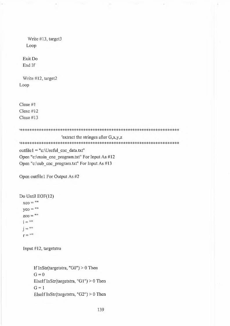
Write #13, target3 Loop
Exit Do End If
Write #12, target2 Loop
Close #1 Close #12 Close #13
'extract the stringes after G,x,y,z
outfilel = "c:\Usefiil_cnc_data.txt"Open "c:\main_cnc_prograrn.txt" For Input As #12 Open "c:\sub_cnc_program.txt" For Input As #13
Open outfilel For Output As #2
Do Until EOF(12) xco = "" yco = "" zeo = "" j =: Im
j = ,m j. _ _ »III
Input #12, targetstra
If InStr(targetstra, "GO") > 0 Then G = 0Elself InStr(targetstra, "Gl") > 0 Then G = 1Elself InStr(targetstra, "G2") > 0 Then
139
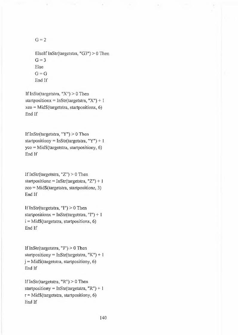
G = 2
Elself InStr(targetstra, "G3") > 0 ThenG = 3ElseG = GEnd If
If InStr(targetstra, "X") > 0 Then startpositionx = InStr(targetstra, "X") + 1 xco = Mid$(targetstra, startpositionx, 6) End If
If InStr(targetstra, "Y") > 0 Then startpositiony = InStr(targetstra, "Y") + 1 yco = Mid$(targetstra, startpositiony, 6) End If
If InStr(targetstra, "Z") > 0 Then startpositionz = InStr(targetstra, "Z") + 1 zeo = Mid$(targetstra, startpositionz, 3) End If
If InStr(targetstra, "I") > 0 Then starlpositionx = InStr(targetstra, "I") + 1 i = Mid$(targetstra, startpositionx, 6) End If
If InStr(targetstra, "J") > 0 Then startpositiony = InStr(targetstra, "K") + 1 j = Mid$(targetstra, startpositiony, 6)End If
If InStr(targetstra, "R") > 0 Then startpositiony = InStr(targetstra, "R") + 1 r = Mid$(targetstra, startpositiony, 6)End If
140
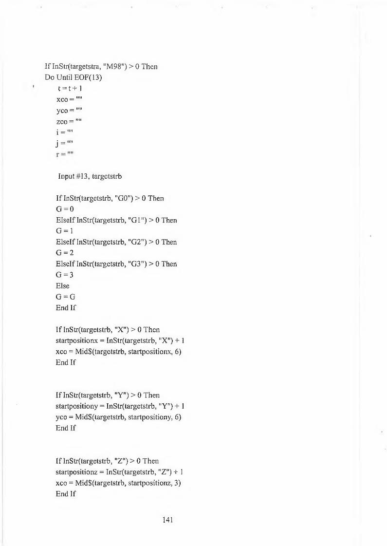
I f InStr(targetstra, "M98") > 0 Then Do Until EOF( 13)
t = t+ 1 xco = "" yco = "" zco = "" j = Im
j = ,m
Input #13, targetstrb
If InStr(targetstrb, "GO") > 0 Then G = 0Elself InStr(targetstrb, "G l") > 0 Then G = 1Elself InStr(targetstrb, "G2") > 0 Then G = 2Elself InStr(targetstrb, "G3") > 0 ThenG = 3ElseG = GEnd If
I f InStr(targetstrb, "X") > 0 Then startpositionx = InStr(targetstrb, "X") + 1 xco = Mid$(targetstrb, startpositionx, 6) End If
I f InStr(targetstrb, "Y") > 0 Then startpositiony = InStr(targetstrb, "Y") + 1 yco = Mid$(targetstrb, startpositiony, 6) End If
If lnStr(targetstrb, "Z") > 0 Then starlpositionz = InStr(targetstrb, "Z") + 1 xco = Mid$(targetstrb, startpositionz, 3) End If
141
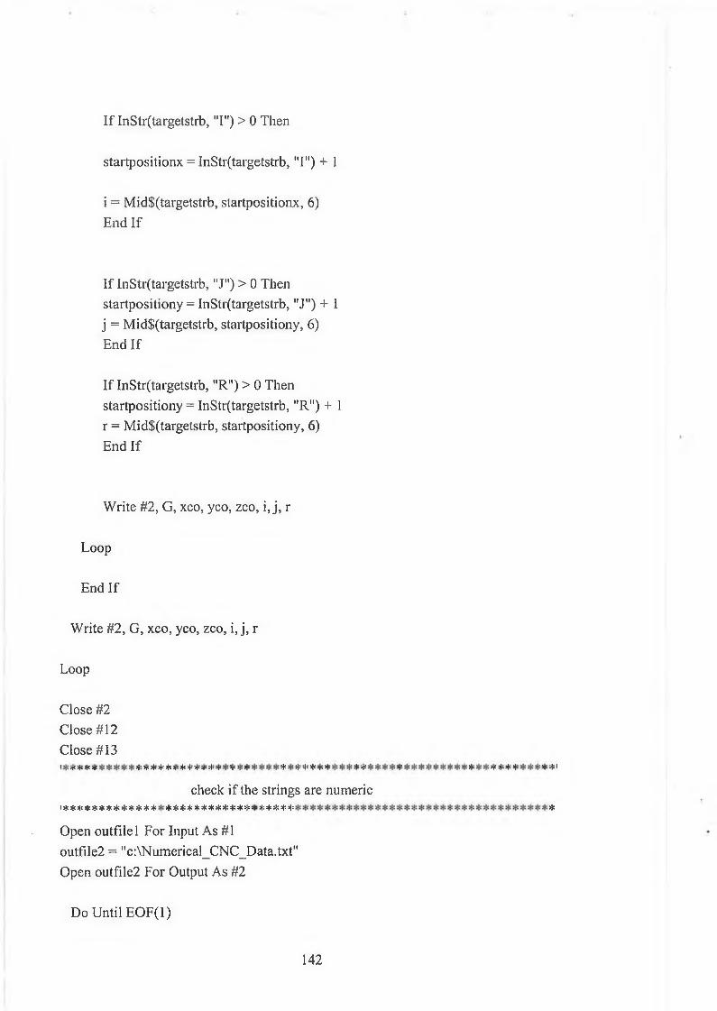
I f InStr(targetstrb, "I") > 0 Then
startpositionx = InStr(targetstrb, "I") + 1
i = Mid$(targetstrb, startpositionx, 6) End If
If InStr(targetstrb, "J") > 0 Then startpositiony = InStr(targetstrb, "J") + 1 j = Mid$(targetstrb, startpositiony, 6) End If
If InStr(targetstrb, "R") > 0 Then startpositiony = InStr(targetstrb, "R") + 1 r = MidS(targetstrb, startpositiony, 6) End If
Write #2, G, xco, yco, zco, i, j, r
Loop
End If
Write #2, G, xco, yco, zco, i, j, r
Loop
Close #2 Close #12 Close #131 « f C «]> /|C Iji jj* JjC ¡j* )Jc 5j{ Sj* 5jC ¡j* 5}» 5)« ¡j* ¡{« 5yC 3{* 3ji ¡J* rJC 3jC *js 3|» !{, »j! JjC 5|» JjC 5|* jf* )|* 5j« ¡» I
check if the strings are numericI jJ: jfc jj: * * * * # # s}: # ♦ H:# # & # * * # * # * * sj: j*: #:{: jfcsJ: jj: #
Open outfilel For Input As #1 outfile2 = "c:\Numerical_CNC_Data.txt"Open outfile2 For Output As #2
Do Until EO F(l)
142
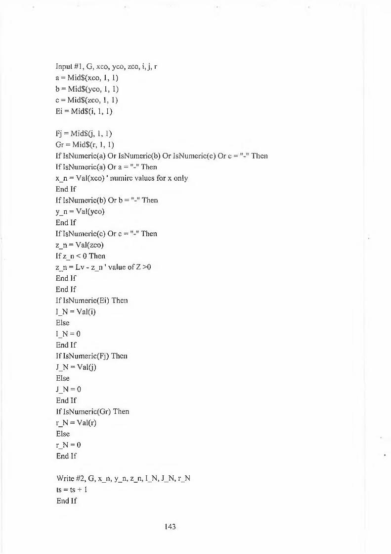
Input #1, G, xco, yco, zco, i ,j , r a = Mid$(xeo, 1,1) b = Mid$(yco, 1,1) c = Mid$(zco, 1,1)Ei = Mid$(i, 1, 1)
Fj = M id$0, 1,1)Gr = Mid$(r, 1,1)If IsNumeric(a) Or IsNumeric(b) Or IsNumeric(c) Or c = ThenIf IsNumeric(a) Or a = Thenx_n = V al(xeo)' numire values for x onlyEnd IfIf IsNumeric(b) Or b = Then y_n = Val(yco)End IfIflsNumeric(c) Or c = Then z_n = Val(zco)If z_n < 0 Thenz_n = Lv - z_n 1 value of Z >0End IfEnd IfIf IsNumeric(Ei) Then I_N = Val(i)Else I_N = 0 End IfIf IsNumeric(Fj) Then J_N = Val(j)Else J_N = 0 End IfIf IsNumeric(Gr) Then r_N = Val(r)Else r_N = 0 End If
Write #2, G, x_n, y_n, z_n, I_N, J_N, r_N ts = ts + 1 End If
143
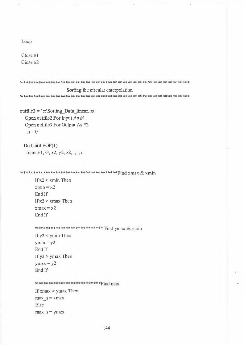
Loop
Close #1 Close #2
• sj: * * * * >*: $ * $: :j: »}: * * * * * * * * * ❖ * * * * * ** * * * :•: & * Jj: * * * * >!•' * * >1: * * * * * * * * H'* * -1: * * * Hi * * * *
1 Sorting the circular enterpolationI«U 4« »1» J < tl* «b *1« vf* *1* * U *1» ^ «1* 4 > « t y < 4 ; 1* •!» >U it 4* J f *fc 4> U* >1« «!■ »1» »!■■J« rj* vfi »]■ FP ip •'p «I« rfi »j» ip ^ if ip ^ *[* rf *p »P M* V v ip V ^ ip V T T T ip 'T ip V 'p »p ip *P *(■ "P ip *p ip <P q» •J* *p ip ip ip *P *P *p *p 4* *1* ip ip ip ip
outfileS = "c:\Sorting_Data_linear.txt"Open outfile2 For Input As #1 Open outfile3 For Output As #2
n = 0
Do Until EOF(l)Input #1, G, x2, y2, z2, i, j, r
* j ( c jJj }{i ¡ji sfisfijj: jjs s|i >Jj s}i s c j j c jJs jji i|i sjc >|i s { i3 } c jJi >|<j|i sfi j|c s}i j|i s}i )J; sJj jJj jjc ) J » j p j X m 3 X ^ iX .m iX ^
If x2 < xmin Then xmin = x2 End IfIf x2 > xinax Then xmax = x2 End If
i*************************** pj^(j ymax & ymin
If y2 < ymin Then ymin = y2 End IfIf y2 > ymax Then ymax = y2 End If
If xmax > ymax Then max_s = xmax Elsemax_s = ymax
144
End If
111 111If xmin < ymin Then m i n s = xmin Else
m i n s = ymin End If
If G = 2 And i o 0 And j o 0 Then r = Sqr(i A 2 + j A 2) xc = x 1 + i yc = y l + j bl = atan2(i, j)12 = x2 - xc J2 = y2 - yc b2 = atan2(12, J2)
If Lc > r Then Lc = r End If
Step = Lc * 180 / (r * (4 * Atn(l)))For b = b l To b2 Step-Step
I f b = 0 Then b = 360 End If
xco = xc + (r * Cos(b * (4 * A tn(l)) /180)) yco = yc + (r * Sin(b * (4 * A tn(l)) / 180)) n = n + 1
Write #2, G, xco, yco, zcox2 = xcoy2 = ycoxl = x2y l = y 2
145

Next
End If
If G = 3 And i o 0 And j <> 0 Then xc = x l + i yc = y l + j
bl = atan2(i, j)
12 = x2 - xc J2 = y2 - yc b2 = atan2(I2, J2)
If L c > r Then Lc = r End If
Step = Lc * 180 / (r * (4 * Atn(l)))For b = b l To b2 Step Step
I f b = 360 Then b = 0 End If
xco = xc + (r * Cos(b * (4 * A tn(l)) /180)) yco = yc + (r * Sin(b * (4 * A tn(l)) / 180)) n = n + 1Write #2, G, xco, yco, zco x2 = xco y2 = yco x l = x2 y l = y2
Next
End If
Appendix D 2 atan2 function
Public Function atan2(X, Y)Pi = 4 * A tn(l)If X > 0 And Y > 0 Then
146
atan2 = Atn(Y / X)Elself X > 0 And Y < 0 Then atan2 = 2 * Pi + Atn(Y / X)Elself X < 0 And Y > 0 Then atan2 = Pi - Atn(Abs(Y / X))Elself X < 0 And Y < 0 Then atan2 = Atn(Abs(Y / X)) + Pi E lself X = 0 And Y > 0 Then atan2 = Pi / 2Elself X = 0 And Y < 0 Then atan2 = 3 / 2 * Pi Elself Y = 0 And X > 0 Then atan2 = 0Elself Y - 0 And X < 0 Then atan2 = PiElself X = 0 And Y = 0 Then atan2 = 0 End Ifatan2 = ISO * atan2 / Pi End Function
Appendix D 3 Decipher the circular interpolation
If r o 0 And (G = 2 Or G = 3) Then ' find the center of the arc r = Val(r)
Step = Lc * ISO / (r * (4 * A tn(l))) xm = (xl + x2) / 2 ym = (yl + y2) / 2 y 12 = (y1 - y 2 ) / 2 x l2 = (xl - x2) / 2
xca = x m + y l 2 * Sqr((r A 2 / (xl2 A 2 + y 12 A 2)) - 1) yea = ym - x l 2 * Sqr((r A 2 / (xl2 A 2 + y 12 A 2)) - 1) xeb = xm - y l2 * Sqr((r A 2 / (xl2 A 2 + y 12 A 2)) - 1) ycb = ym + x l2 * Sqr((r A 2 / (xl2 A 2 + y 12 A 2)) -1)
dxla = xl - xca
147
dyla — yl - yeaGa 1 = atan2(dx 1 a, dy 1 a)
dx2a = x2 - xca dy2a = y2 - yea Ga2 = ataii2(dx2a, dy2a)
dxlb = xl - xeb dylb = yl - ycb Gbl = atan2(dxlb, dylb)
dx2b = x2 - xeb dy2b = y2 - ycb Gb2 = atan2(dx2b, dy2b)
I f G = 3 Then
DGa = Ga2 - Gal DGb = Gb2 - Gbl
I f DGa < 0 Then Ga2 = Ga2 + 360 DGa — Ga2 - G al End IfIf DGb < 0 Then Gb2 = Gb2 + 360 DGb = Gb2 - Gbl End If
If (Abs(DGa) > 180 And Ri = "-") Or (Abs(DGa) <= 180 And Ri o "-") Then For Ga = Gal To Ga2 Step Step X = xca + (r * Cos(Ga * Pi /180))Y = yea + (r * Sin(Ga * Pi / 180))Write #2, G, X, Y, z2n = n + 1 Next GaElself (Abs(DGb) > 180 And Ri = Or (Abs(DGb) <= 180 And Ri o "-")
ThenFor Gb = Gbl To Gb2 Step Step X = xeb + (r * Cos(Gb * Pi /180))Y = ycb + (r * Sin(Gb * Pi / 180))
148
Write #2, G, X, Y, z2 n = n + 1 Next Gb End If
Elself G = 2 Then
DGa = Ga2 - Gal DGb = Gb2 - Gbl
If DGa > 0 Then Ga2 = Ga2 - 360 DGa = Gal - Ga2 End IfI f DGb > 0 Then Gb2 = Gb2 - 360 DGb = Gbl - Gb2 End If
If (Abs(DGa) > 180 And Ri = Or (Abs(DGa) <= 180 And Ri <> Then For Ga = G al To Ga2 Step -Step r = Sqr((xca - x l) A 2 + (yea - y l) A 2)X = xca + (r * Cos(Ga * Pi /180))Y = yea + (r * Sin(Ga * Pi / 180))Write #2, G, X, Y, z2n = n + 1 Next GaElself (Abs(DGb) > 180 And Ri = "-") Or (Abs(DGb) <= 180 And Ri <> "-")
ThenFor Gb = Gbl To Gb2 Step -Step X = xeb + (r * Cos(Gb * Pi / 180))Y = ycb + (r * Sin(Gb * Pi / 180))Write #2, G, X, Y, z2n = n + 1 Next Gb
End If End If
End If
149
xl = x2 y l = y 2 n = n + 1
Write #2, G, x2, y2, z2
Close #1 Close #2
Appendix D4 Drawing CNC tool path
Public Sub Drawing CNCO
Call Drawaxis
xl = 0 y l = 0 z l = 0
Open outfile3 For Input As #1
Do Until EOF(l)
Input #1, G, x2, y2, z2If z o z2 And G o 0 ThenCall Picture l.ClsCall DrawaxisEnd IfDoEvents
Call slow
If G = 0 ThenPicture 1.Line (xl, yl)-(x2, y2), Filtring_color ElsePicturel.Line (xl, yl)-(x2, y2), Deposition_color End If
150
x l = x2
y l = y 2I f z2 o 0 Then z = z2 End If
Loop
Close #1
End Sub
Appendix D4 simulate the deposition of wax
Public Sub simulate()
Call Drawaxis
Open outfile3 For Input As #1Open "c:\positions_for_filtring.txt" For Output As #4 'positions_for filtring Open "c:\deposition_positions.txt" For Output As #5 'deposition_positions
Input #1, G, wx. wy, z2 z = z2
Picture l.FillStyle = FillStyle_DepPicture l.FillColor = Deposition_colorPicture 1.Circle (wx, wy), D_drop / 2, Deposition_colorWrite #4, wx, wy, z2Write #5, wx, wy, z2
Do Until E0F(1)
Input #1, G, x2, y2, z2
If z o z2 And G o 0 ThenCall Picturel.ClsCall DrawaxisEnd IfDoEvents
151
Dx = x2 - wx
Dy = y2 - wydt = (Dx A 2 + Dy A 2) A (1 / 2)
If Abs(dt) >= LD And G o 0 Then mn = dt / LD 'number o f motion
For k = 1 To mn I f Dx = 0 And Dy <> 0 Then wy = wy + LD * Dy / dt
E lself Dx <> 0 And Dy = 0 Then wx = wx + LD * Dx / dt
E lself Dy <> 0 And Dx <> 0 Then wx = wx + LD * Dx / dt wy = wy + LD * Dy / dt End I fPicturel.Circle (wx, wy), D d r o p / 2, Deposition_color Write #4, wx, wy, z2 Write #5, wx, wy, z2
dep_num = dep_num + 1 Call slow
Next k
Elself G = 0 And Abs(dt) o 0 Then Picturel.Line (wx, wy)-(x2, y2), Filtring_color wx = x2 wy = y2
End If
I f G o 0 Then z = z2 End If
Loop
Close #1 Close #4
152

Close #5
End Sub
Appendix D5 Correct
Private Sub Correct_Click() outfile5 = "c:\positions_for_filtring.txt"On Error GoTo HandleErrors HandleErrors:
I f Err .Number = 75 ThenintResponse = MsgBox("file not found", vbOKOnly, "Invalid Path")Exit Sub End If
Listl.Visible = False dep_num = 0
Call Picturel.Cls Call Drawaxis
Open outfile5 For Output As #4 'positions_for filtringOpen "c:\deposition_positions.txt" For Output As #5 'deposition_positions Open outfile3 For Input As #1
Input #1, G, x l, y l, zlz = zl
Do Until EOF(l)
Input #1, G, x2, y2, z2
If z o z2 And G o 0 ThenCall Picturel.ClsCall DrawaxisEnd IfDoEvents
153
Dx = x2 - x l
Dy = y2 - y ldt = (Dx A 2 + Dy A 2) A (1 / 2)
I f Abs(dt) >= LD And G o 0 Thenmn = dt / LD 'number o f steps for this motionw x = x l ' starting from the last origenal position in xwy = y l ' starting from the last origenal position in y
Picture l.FillStyle = FillStyle_DepPicturel.FillColor = Deposition_coiorPicture 1.Circle (wx, wy), D drop / 2, Deposition_colorWrite #4, wx, wy, z2Write #5, wx, wy, z2dep_num = dep_num + 1Call slow
For k = 1 To mn If Dx = 0 And Dy o 0 Then wy = wy + LD * Dy / dt Elself Dx o 0 And Dy = 0 Then wx = wx + LD * Dx / dt Elself Dy o 0 And Dx o 0 Then wx = wx + LD * Dx / dt wy = wy + LD * Dy / dt End If
Picture l.FillStyle = Fi l lStyleDepPicturel.FillColor = Deposition_colorPicture 1.Circle (wx, wy), D_drop / 2, Deposition_colorWrite #4, wx, wy, z2Write #5, wx, wy, z2depjium = dep_num + 1Call slow
Nextk xl = x2 y l = y 2
154
Elself Abs(dt) < LD And G = 1 Then
xl = x2 y l = y 2
Elself G = 0 And Abs(dt) <> 0 Then Picture 1.Line (x l, yl)-(x2, y2)
x l = x2 y l = y 2
End If
If G o 0 Then z — z2 End If
Loop
Close #1 Close #4 Close #5
End Sub
Appendix D6 filtering algorithm
Public 0outfile6 = "c:\deposition_positions,txt" mainfnn.Listl. Visible = Falsekecjuest")yal(InPUtB0X("Enter the minimun distance bettwen the droplets", "Input
On Error GoTo HandleErrors
Open outfileS For Input As #5 Input #5, x l, y l, z l
Open outfile6 For Output As #6 Write #6, x l, y l, zl Close #6
155

Call mainfnn.Picturel.Cls Call Drawaxismainfrm.Picturel.FillStyle = FillStyle_Dep mainfrm.Picturel .FillColor = Deposilion_color mainfrm.Picturel.Circle (xl , yl), D_drop /2 , Deposi t ioncolor
z = zl
Do Until EOF(5)
DoEvents Er = 0 Call slow
Input #5, x l, y l, zl
If z o zl Then Call mainfrm.Picture l.Cls Call Drawaxis End If
Open outfile6 For Input As #6
Do Until E0F(6)
Input #6, x2, y2, z2
d = Sqr((x2 - x l) A 2 + (y2 - y l) A 2)
If d < Lmin And z l = z2 Then Er = Er + 1
End If
Loop
Close #6
I f E r o O T h e n
156
mainfrm.Picture l.FillStyle = FillStylefiltr
mainfrm.Picture 1 .FillColor = Filtring color mainfrm.Picture 1 .Circle (x l, y l) , D_drop / 2, Filtring_color
Elself Er = 0 Then
Open outfile6 For Append As #6 Write #6, x l, y l, zl Close #6
mainfrm.Picture LFillStyle = Fi l lStyleDep mainfrm.Picture 1 .FillColor = Deposition_color mainfrm.Picture 1.Circle (xl , yl ) , D drop / 2, Deposition_color
End If
z = zl Loop
Close #5
HandleErrors:If Err.Number = 75 ThenintResponse = MsgBox("file not found", vbOKOnly, "Invalid Path")Exit SubElseExit Sub
End If
End Sub
157

PC23 RESET, READ, WRITE DRIVERS
The following routines will compile under Borland or Microsoft C.They are intended to demonstrate basic communication routines in C.
#include <stdio.h>#include <conio.h>#include <stdlib.h>#include <dos.h>
#defmeFAIL 0X20#defxne BIT2MASK 0X04 #defme READY 0X16 #defineCB 0X60#defmeIDB_M 0X10#defme CHAR READY 0X70#define ODB 0X8#define ACK 0XE0#defme ALDONE 0X02 #defme BADADDR 0XFF #defme HALT (CB | BIT2MASK)#defme RESTART 0x40 /* byte to restart the pc21 */void initialize (void);void writech (char);char readch (void);void writecmd (char *s);void readanswer (char *s);void callstayO;int axis, address ; /* normally 300 hex */
int main()
{char *message,*answer;FILE *fp; int ch; char * input;int true=0,start=0,end=0; int counter^O.i;
Appendix F CAM/RP
158
int a;char *fileN;answei-"";m essage-"';/*if(argc!=2)
{printf("Please Enter command as: File [data file name]"); return 0;
}*/
/*if((fp=fopen (argv[ 1 ],"r"))=N U LL)*/
/printf("Enter the file Name: \n");scanf("%s",fileN);printf(fileN);*/fileN=("c:\\drop 1 .txt"); if((fp=fopen (fileN ,"r"))=NULL)
{printf("Unable to open the file."); return 0;
}
initialize (); /* RESET THE PC23 */
printf("\n The following program example demonstrates the basic"); printf("\n use o f RESET, READ, and WRITE C drivers for the PC23."); printf("\n\n The C source file is motonn.CAn");
while((ch=fgetc(fp))!=EOF)
{if(ch==34)
{if(tru e= 0 ) {true=T ;start= 1 ;end=0;} else
{ true = 0;start=0;end=l;} if(true == 0)
free(input);
}
159

if(start== 1 )
{input=(char *) malloc(2Q0*sizeof(char));countei-O;start=0;
}if (true = 1)
{input[counter]=ch;
counter++;
}
if (e n d = l)
{printf("\ii"); input[c ounter]=34 ;message =(char *) malloc((counter) * sizeof(char)); /* malloc
is used for memory allocation */for(i=0 ; i <counter ; i++) message[i]=input[i]; printf("%s", message); writecmd(message);while((inportb(address+l) & ALDONE) != ALDONE);readanswer(answer);prinlf("\n%s", answer);answer="";m essage-'";
}
fclose(fp); /*closing the open file */
/*message=" 3PR "; /* AXIS 3 POSITION * /
/*writecmd(message); readanswer(ans wer) ; printf("\n "); print f(answer); printf("\n");*/
return 0;
160
}
INITIALIZE: RESET THE PC23 BOARD. ASSURING THAT THE BOARD IS READY TO ACCEPT COMMANDS FROM THE USER PROGRAM.
void initialize ()
{char i;int status_addr=0; unsigned char statbyte;/*printf("\n\n");printf("Enter the Decimal value Board Address for the PC-23 :");/*scanf("%d",&address);*/address=768;if ((address < 768) || ( address >812))
{printf ("\n\nlnvalid address, check PC-23 dipswitches\n\n"); exit(l);
}status_addr=address+l; outp(status_addr,HALT);
/* initialize procedure */ while(!((stalbyte=inp(status_addr)) & FAIL) ); if(statbyte==BADADDR)
cprintf ("\n\nlnvalid address, check PC-23 dipswitches\n\n"); exit(l);
}outp(status_addr, RESTART); outp(status_addr,CB);while( ( (statbyte:=inp(status_addr)) & READY) != READY );
}
161
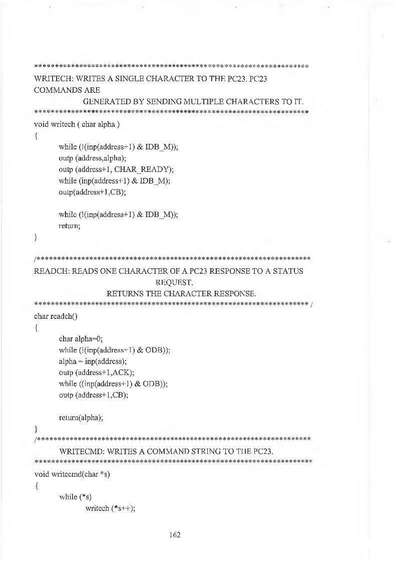
*L* *1» *1* »1* ■!* il# '!> «1* +L* *tj «L kb *J> *N hU *1* *1* vl» 1* ■!* >1* 1* V% »]■ *1« «1* vL* *1» *1* «1* 4/ *!< k1* d « vtj O« J# »t# kl« «1« k|j k]r iU J j d * «U *1« «J# fcl* hb hlj J , if, if. *f« «fa kf< kfa J«'I* *1' 'T* 'r T T I 1 T T M* ^ T n 1 T 'P 'i* I* *i* 'I ’ 'I* 'P "7* v 'p 'I* V *T* T* 'I ' '1 ' *|* ■i' V q* 'p * |' ■!* » !' *i* 'I* '1^ *1« ■]« ifi rf’ *j* -j* »p* Jj; ijs Pfi if« rf> #1» ¿¡» if! p> -p
WRITECH: WRITES A SINGLE CHARACTER TO THE PC23. PC23 COMMANDS ARE
GENERATED BY SENDING MULTIPLE CHARACTERS TO IT.ijs i j j jjc j j i jj" j | j jj* ^ *|» l | j jJj j j j jJj j| j jj* jJj jj* j|* jj j jj* *|« *|« *J< j| j *|> kj* *|# «1# (|d ^ kjx tja tja j|# «|# a|«
void writech ( char alpha )
{while (!(inp(address+l) & IDB_M)); outp (address,alpha); outp (address+1, CHAR_READY); while (inp(address+l) & IDB_M); outp(address+l ,CB);
while (!(inp(address+l) & IDB_M)); return;
}
READCH: READS ONE CHARACTER OF A PC23 RESPONSE TO A STATUSREQUEST.
RETURNS THE CHARACTER RESPONSE.
char readch()
{char alpha=0;while (!(inp(address+l) & ODB)); alpha = inp(address); outp (address+l,ACK); while ((inp(address+l) & ODB)); outp (address+1,CB);
retum(alpha);
}
WRITECMD: WRITES A COMMAND STRING TO THE PC23.
void writecmd(char *s)
{while (*s)
writech (*s++);
162

return;
}M . Up. sfi ifc Jjf »■: if : sjs ¡$: aft sj: >f; af: sfc ¡fc aj: ifc Jfc sjj:: sjc :&r i f : sjc jfc s[i sj? SIS ¡it sfc 3*; =}> sf; ifc if« sfs. sft s$S if ; :jfi }Ji s(i ?J< j j i :>j« ;5jt & ' : f i 3$: ?[: : j: 3§t s{; $ s{: i f : ;- i i j i
READANSWER: READS A COMPLETE PC23 STATUS REQUEST RESPONSESTRING.
# a{ i >1; >ji jfc j}£ : j ; )f: s{c sjc :{c jje $ s}c s|e :fc :jc j}c # -J: jJ: jje ;i* $ $ ' $ $ $ $ $ $ $ $ $ $ $ $ $ # $ ' $ # $ $ $ # $ $ $ # #
void readanswer (char *s)
{while ((*s++ = readchO) != 13);*s = ,\0’; return;
}void callstay()
{delay(2000);
}
163