c1,1 estimates for solutions of a problem of alexandrov

C1,1 Estimates for Solutionsof a Problem of Alexandrov

PENGFEI GUANMcMaster University

AND

YANYAN LIRutgers University

0 Introduction

For n ≥ 2, let Mn be a finite convex, not necessarily smooth, hypersurfacein Euclidean spaceRn+1 containing the origin. More precisely,Mn is theboundary of some convex domain inRn+1 containing a neighborhood of theorigin. We writeMn = {R(x) = ρ(x)x | x ∈ Sn}, whereρ is a functionfrom Sn to R+. Let ν : Mn → Sn denote the generalized Gauss map, namely,ν(Y ) is the set of outward unit normals to supporting hyperplanes ofMn atY . The integral Gaussian curvature ofMn is defined by

µ(F ) = |ν(R(F ))| for all Borel setsF ⊂ Sn .

It is clear thatµ is a nonnegative, completely additive function on the Borelsets ofSn. For any setF ⊂ Sn, let Cone(F ) = {tX | X ∈ F, t ≥ 0} bethe cone generated byF . For any coneC ⊂ Rn+1, let C∗ = {X ∈ Rn+1 |X · Y ≤ 0, ∀Y ∈ C} be the dual cone.F ∗ = (Cone(F ))∗ ∩ Sn is the dualangle. The following theorem was obtained by A. D. Alexandrov in [1] (seealso [2] and [24] for exposition):

THEOREM A A necessary and sufficient condition for a nonnegative, com-pletely additive functionµ on the Borel sets ofSn to be the integral Gaussiancurvature of some finite convex hypersurface in Euclidean spaceRn+1 con-taining the origin is the following:

(A1) µ(Sn) = |Sn| and

(A2) for every convex subsetF of Sn, µ(F ) < |Sn| − |F ∗|.

Such a hypersurface is unique up to a homothetic transformation.

WhenMn is C2, it is clear that|ν(R(F ))| =∫R(F ) κ, whereκ is the

Gauss-Kronecker curvature ofMn. On the other hand, when the density

Communications on Pure and Applied Mathematics, Vol. L, 0789–0811 (1997)c© 1997 John Wiley & Sons, Inc. CCC 0010–3640/97/080789-23

790 P. GUAN AND Y. Y. LI

of µ is a smooth positive function onSn, the solution to the Alexandrovproblem is smooth; see [24] and [23]. The main difficulty in establishingthis smoothness result is in establishingC2,α estimates fromC2 estimatesfor elliptic Monge-Ampère equations, which is the same analytically as inthe Weyl problem and the Minkowski problem ([22, 9] and the referencestherein). For such regularity results and more recent developments, please see[22, 21, 8, 9, 18, 10, 12, 6, 3, 20, 19] and the references therein. A prioriC0

estimates of solutions to the Alexandrov problem are studied in [25], where anecessary and sufficient condition was given.

It is natural to ask whether the solutions to the Alexandrov problem are al-ways smooth when the density ofµ is smooth but onlynonnegative. Herewe encounter certaindegenerateMonge-Ampère equations. Regularity ofsolutions to degenerate Monge-Ampère equations have been investigated in[5, 26, 7, 4, 14, 15] and the references therein. We show in this paper thatwhen the density ofµ is smooth and nonnegative, solutions to the Alexandrovproblem are at leastC1,1 in dimensionsn = 2, 3. For higher dimensions, wehave the same conclusion under some further hypotheses on the density func-tion of µ. We also show that, in general, one cannot conclude that the solutionis smooth even though the density ofµ is smooth. In fact, we have pro-duced someµ with smooth, nonnegative density functions where the solutionis merelyC2,2/n(Sn). In particular, it is notC3.

In an earlier work [16], we studied the Weyl problem with nonnegativeGauss curvature and established aC1,1 regularity result. See also [17] for anindependent proof. The equation we have there is a certain two-dimensionaldegenerate Monge-Ampère equation.

Let k be some nonnegative function defined onSn. We set

µ(F ) =∫Fk(0.1)

for all Borel setsF of Sn. It is clear thatµ is a nonnegative, completelyadditive function on the Borel sets ofSn.

THEOREM 0.1 (a) Let k ∈ C1,1(S2) be a nonnegative function, andµ begiven by(0.1). Suppose thatµ satisfies(A1) and (A2); then there existssomeC1,1 finite convex surfaceM2 havingµ as its integral Gaussiancurvature.

(b) Let k ∈ C3,1(S3) be a nonnegative function, andµ be given by(0.1).Suppose thatµ satisfies(A1) and (A2); then there exists someC1,1 finiteconvex surfaceM3 havingµ as its integral Gaussian curvature.

Such a hypersurface is unique up to a homothetic transformation.

A PROBLEM OF ALEXANDROV 791

For higher dimensions, we need some additional hypotheses to concludethere isC1,1 regularity. We introduce the following condition forn ≥ 2:

Condition I. k ∈ C0,1(Sn) is nonnegative and, for some constantA > 0,satisfies

(i) ∆(k1/(n−1)) ≥ −A on Sn in the distribution sense and

(ii) |∇(k1/(n−1))| ≤ A on Sn.

It is clear that for a nonnegative functionk ∈ C1,1(Sn), part (i) of condi-tion I is equivalent to

(n−1)k(x)∆k(x)−(n−2)|∇k(x)|2 ≥ −(n−1)2Ak(x)2−1/(n−1) ∀x ∈ Sn ,

and part (ii) of condition I is equivalent to

|∇k(x)| ≤ (n− 1)Ak(x)(n−2)/(n−1) ∀x ∈ Sn .

THEOREM 0.2 For n ≥ 2, let k satisfy conditionI, andµ be given by(0.1).Suppose thatµ satisfies(A1) and(A2); then there exists someC1,1 finite convexsurfaceMn havingµ as its integral Gaussian curvature. Such a hypersurfaceis unique up to a homothetic transformation.

We also introduce another condition.

Condition II . k ∈ C1,1(Sn) is nonnegative and, for some constantA > 0,satisfies

2k(x)∆k(x)− 3|∇k(x)|2 ≥ −Ak(x)2−1/(n−1) ∀x ∈ Sn .

THEOREM 0.3 For n ≥ 2, let k ∈ C2,α(Sn) (0 < α < 1) satisfy conditionII ,and µ be given by(0.1). Suppose thatµ satisfies(A1) and (A2); then thereexists someC1,1 finite convex surfaceMn havingµ as its integral Gaussiancurvature. Such a hypersurface is unique up to a homothetic transformation.

Concerning conditions I and II, we make the following remarks:

REMARK 0.1 Forn = 2, all nonnegative functionsk ∈ C1,1(S2) satisfy con-dition I. Forn = 3, all nonnegative functionsk ∈ C3,1(S3) satisfy condition I.

REMARK 0.2 Forn ≥ 2, suppose that condition I is satisfied byk1 andk2.Then condition I is satisfied byk1k2 andα1k1 + α2k2, whereα1 andα2 areany nonnegative constants.


REMARK 0.3 Forn ≥ 2, let k =∑Nj=1 f

mjj for someN ∈ Z+, mj ≥ n− 1,

fj ∈ C1,1(Sn), and fj(x)mj ≥ 0 ∀x ∈ Sn, 1 ≤ j ≤ N . Then k satisfiescondition I.

REMARK 0.4 Forn ≥ 2, suppose thatk ∈ C2(Sn) is nonnegative and hasnondegenerate Hessian at points wherek = 0. Thenk satisfies condition II.

REMARK 0.5 Then− 1 exponent in condition I is sharp forC1,1 regularityto the Dirichlet problem of degenerate Monge-Ampère equations. See [27]and [14].

Remarks 0.1 through 0.3 and some further properties will be discussed inSection 2. Most of them are fairly elementary except for the casen = 3in Remark 0.1. Theorem 0.1 follows immediately from Theorem 0.2 andRemark 0.1.

1 C1,1 Estimates and the Proof of Theorem 0.2–0.3

In this section, we first establish some a priori estimates (Theorem 1.1). Thenwe establish Theorem 0.2–0.3 by using Theorem 1.1.

THEOREM 1.1 (a) For n ≥ 2, let ρ ∈ C4,α(Sn), let k ∈ C2,α(Sn) (0 <α < 1) satisfy conditionI, and let µ, given by(0.1), be the integralGaussian curvature ofMn = {R(x) = ρ(x)x | x ∈ Sn}. Then

‖ρ‖C2(Sn) ≤ C ,

whereC depends only onn, maxSn ρ/minSn ρ, maxSn |∇ρ|/minSn ρ,A, andmaxSn k.

(b) For n ≥ 2, let k satisfy conditionII ; then

‖ρ‖C2(Sn) ≤ C ,

whereC depends only onn,maxSn ρ/minSn ρ,maxSn |∇ρ|/minSn ρ,A,and maxSn k.

Let k be some nonnegative function onSn, andµ(F ) be as in (0.1). Lete1, . . . , en be some smooth local frame field onSn, and let∇ denote thecovariant differentiation. Letσij = 〈ei, ej〉 denote the metric onSn, σij

denote its inverse, andσ = det(σij). ForMn = {R(x) = ρ(x)x | x ∈ Sn} to


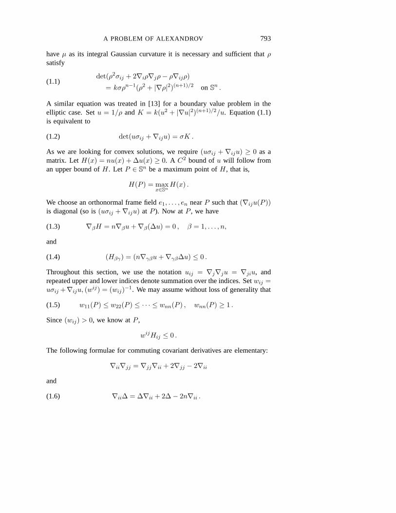
haveµ as its integral Gaussian curvature it is necessary and sufficient thatρsatisfy

det(ρ2σij + 2∇iρ∇jρ− ρ∇ijρ)

= kσρn−1(ρ2 + |∇ρ|2)(n+1)/2 on Sn .(1.1)

A similar equation was treated in [13] for a boundary value problem in theelliptic case. Setu = 1/ρ andK = k(u2 + |∇u|2)(n+1)/2/u. Equation (1.1)is equivalent to

det(uσij +∇iju) = σK .(1.2)

As we are looking for convex solutions, we require(uσij + ∇iju) ≥ 0 as amatrix. LetH(x) = nu(x) + ∆u(x) ≥ 0. A C2 bound ofu will follow froman upper bound ofH. Let P ∈ Sn be a maximum point ofH, that is,

H(P ) = maxx∈Sn

H(x) .

We choose an orthonormal frame fielde1, . . . , en nearP such that(∇iju(P ))is diagonal (so is(uσij +∇iju) at P ). Now atP , we have

∇βH = n∇βu+∇β(∆u) = 0 , β = 1, . . . , n,(1.3)

and

(Hβγ) = (n∇γβu+∇γβ∆u) ≤ 0 .(1.4)

Throughout this section, we use the notationuij = ∇j∇ju = ∇jiu, andrepeated upper and lower indices denote summation over the indices. Setwij =uσij +∇iju, (wij) = (wij)−1. We may assume without loss of generality that

w11(P ) ≤ w22(P ) ≤ · · · ≤ wnn(P ) , wnn(P ) ≥ 1 .(1.5)

Since(wij) > 0, we know atP ,

wijHij ≤ 0 .

The following formulae for commuting covariant derivatives are elementary:

∇ii∇jj = ∇jj∇ii + 2∇jj − 2∇ii

and

∇ii∆ = ∆∇ii + 2∆− 2n∇ii .(1.6)


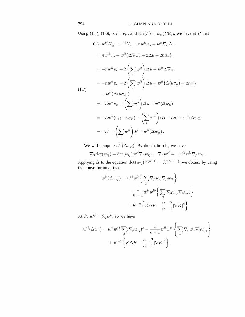
Using (1.4), (1.6),σij = δij , andwij(P ) = wii(P )δij , we have atP that

0 ≥ wijHij = wiiHii = nwiiuii + wii∇ii∆u

= nwiiuii + wii{∆∇iiu+ 2∆u− 2nuii}

= −nwiiuii + 2

(∑i

wii)

∆u+ wii∆∇iiu

= −nwiiuii + 2

(∑i

wii)

∆u+ wii{∆(uσii) + ∆uii}

−wii(∆(uσii))

= −nwiiuii +

(∑i

wii)

∆u+ wii(∆wii)

= −nwii(wii − uσii) +

(∑i

wii)

(H − nu) + wii(∆wii)

= −n2 +

(∑i

wii)H + wii(∆wii) .

(1.7)

We will computewii(∆wii). By the chain rule, we have

∇β det(wij) = det(wij)wij∇βwij , ∇βwij = −wikwlj∇βwkl .

Applying ∆ to the equationdet(wij)1/(n−1) = K1/(n−1), we obtain, by usingthe above formula, that

wij(∆wij) = wikwlj{∑

β

∇βwij∇βwlk}

− 1n− 1

wijwlk{∑

β

∇βwij∇βwlk}

+K−2{K∆K − n− 2

n− 1|∇K|2

}.

At P , wij = δijwii, so we have

wii(∆wii) = wiiwjj∑β

(∇βwij)2 − 1n− 1

wiiwjj

∑β

∇βwii∇βwjj

+K−2

{K∆K − n− 2

n− 1|∇K|2

}.


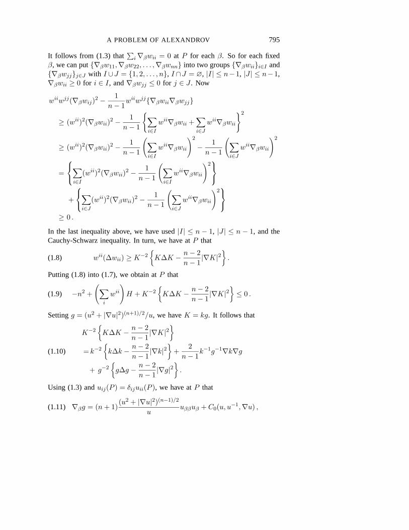
It follows from (1.3) that∑i∇βwii = 0 at P for eachβ. So for each fixed

β, we can put{∇βw11,∇βw22, . . . ,∇βwnn} into two groups{∇βwii}i∈I and{∇βwjj}j∈J with I ∪J = {1, 2, . . . , n}, I ∩J = ∅, |I| ≤ n−1, |J | ≤ n−1,∇βwii ≥ 0 for i ∈ I, and∇βwjj ≤ 0 for j ∈ J . Now

wiiwjj(∇βwij)2 − 1n− 1

wiiwjj{∇βwii∇βwjj}

≥ (wii)2(∇βwii)2 − 1n− 1

{∑i∈I

wii∇βwii +∑i∈J

wii∇βwii}2

≥ (wii)2(∇βwii)2 − 1n− 1

(∑i∈I

wii∇βwii)2

− 1n− 1

(∑i∈J

wii∇βwii)2

=

∑i∈I

(wii)2(∇βwii)2 − 1n− 1

(∑i∈I

wii∇βwii)2

+

∑i∈J

(wii)2(∇βwii)2 − 1n− 1

(∑i∈J

wii∇βwii)2

≥ 0 .

In the last inequality above, we have used|I| ≤ n − 1, |J | ≤ n − 1, and theCauchy-Schwarz inequality. In turn, we have atP that

wii(∆wii) ≥ K−2{K∆K − n− 2

n− 1|∇K|2

}.(1.8)

Putting (1.8) into (1.7), we obtain atP that

−n2 +

(∑i

wii)H +K−2

{K∆K − n− 2

n− 1|∇K|2

}≤ 0 .(1.9)

Settingg = (u2 + |∇u|2)(n+1)/2/u, we haveK = kg. It follows that

K−2{K∆K − n− 2

n− 1|∇K|2

}= k−2

{k∆k − n− 2

n− 1|∇k|2

}+

2n− 1

k−1g−1∇k∇g

+ g−2{g∆g − n− 2

n− 1|∇g|2

}.

(1.10)

Using (1.3) anduij(P ) = δijuii(P ), we have atP that

∇βg = (n+ 1)(u2 + |∇u|2)(n−1)/2

uuββuβ + C0(u, u−1,∇u) ,(1.11)


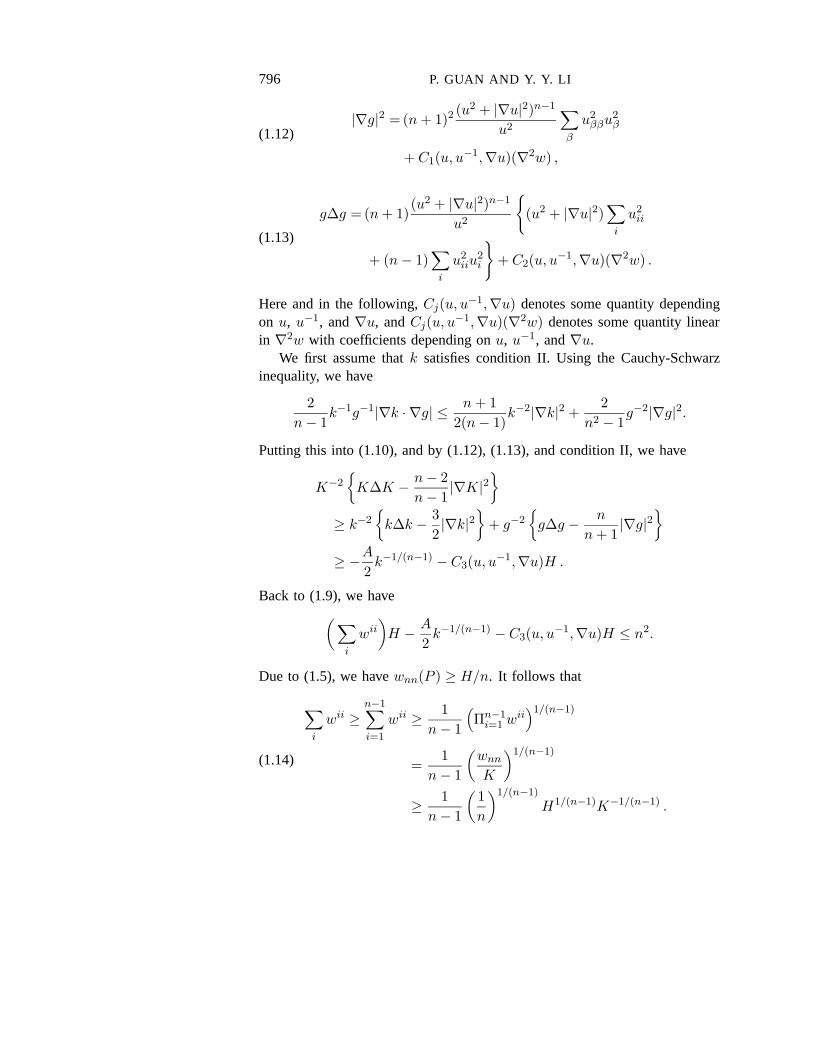
|∇g|2 = (n+ 1)2 (u2 + |∇u|2)n−1

u2

∑β

u2ββu

2β

+ C1(u, u−1,∇u)(∇2w) ,

(1.12)

g∆g = (n+ 1)(u2 + |∇u|2)n−1

u2

{(u2 + |∇u|2)

∑i

u2ii

+ (n− 1)∑i

u2iiu

2i

}+ C2(u, u−1,∇u)(∇2w) .

(1.13)

Here and in the following,Cj(u, u−1,∇u) denotes some quantity dependingon u, u−1, and∇u, andCj(u, u−1,∇u)(∇2w) denotes some quantity linearin ∇2w with coefficients depending onu, u−1, and∇u.

We first assume thatk satisfies condition II. Using the Cauchy-Schwarzinequality, we have

2n− 1

k−1g−1|∇k · ∇g| ≤ n+ 12(n− 1)

k−2|∇k|2 +2

n2 − 1g−2|∇g|2.

Putting this into (1.10), and by (1.12), (1.13), and condition II, we have

K−2{K∆K − n− 2

n− 1|∇K|2

}≥ k−2

{k∆k − 3

2|∇k|2

}+ g−2

{g∆g − n

n+ 1|∇g|2

}≥ −A

2k−1/(n−1) − C3(u, u−1,∇u)H .

Back to (1.9), we have(∑i

wii)H − A

2k−1/(n−1) − C3(u, u−1,∇u)H ≤ n2.

Due to (1.5), we havewnn(P ) ≥ H/n. It follows that

∑i

wii ≥n−1∑i=1

wii ≥ 1n− 1

(Πn−1i=1 w

ii)1/(n−1)

=1

n− 1

(wnnK

)1/(n−1)

≥ 1n− 1

(1n

)1/(n−1)H1/(n−1)K−1/(n−1) .

(1.14)


Therefore

1n− 1

(1n

)1/(n−1)K−1/(n−1)H1+1/(n−1)

− A

2k−1/(n−1) − C3(u, u−1,∇u)H ≤ n2 ,

which yields

H

{1

n− 1

(1n

)1/(n−1)H1/(n−1) − k1/(n−1)C4(u, u−1,∇u)

}

≤ A

2+ n2k1/(n−1).

We conclude from the above that

H(P ) ≤ C5(u, u−1,∇u, k,A) .

This gives an upper bound formaxSn H.Whenk satisfies condition I, it follows from (1.11) that

2n− 1

|∇k · ∇g| ≤ 2n− 1

A2k1−1/(n−1)C6(u, u−1,∇u)H .

Putting the above into (1.10) and using the above, (1.12), (1.13), and condi-tion I, we have

K−2{K∆K − n− 2

n− 1|∇K|2

}≥ k−2

{k∆k − n− 2

n− 1|∇k|2

}− 2n− 1

A2k−1/(n−1)C6(u, u−1,∇u)H

+ g−2{g∆g − n− 2

n− 1|∇g|2

}≥ − A1

n− 1k−1/(n−1) − 2

n− 1A2k

−1/(n−1)C6(u, u−1,∇u)H

− C7(u, u−1,∇u)H .

(1.15)

Putting (1.15) into (1.9), we obtain (usingH(P ) ≥ 1) that∑i

wiiH − C8(u, u−1,∇u,A1, A2)k−1/(n−1)H − C9(u, u−1,∇u)H ≤ 0 ,

namely,∑i

wii ≤ C8(u, u−1,∇u,A1, A2)k−1/(n−1) + C9(u, u−1,∇u) .


By (1.14), we conclude

H1/(n−1) ≤ C10(u, u−1,∇u,A1, A2) + C11(u, u−1,∇u)k1/(n−1) .

This provides an upper bound formaxSn H. We have thus proved Theorem 1.1.In the following, we will use Theorem 1.1 to prove Theorem 0.2–0.3. We

make some preliminary observations concerningC0 a priori estimates.

PROPOSITION1.1 For n ≥ 2, 1 < p < ∞, suppose thatk ∈ Lp(Sn) issome nonnegative function such thatµ, given by(0.1), satisfies(A1) and (A2).Let {kj} be a sequence of nonnegative functions converging strongly tok intheLp(Sn) norm, and letµj satisfy(A1). Thenµj satisfies(A2) for j largeenough. Furthermore, for some constantC depending only onk, we have

lim supj→∞

maxSn ρjminSn ρj

≤ C ,

whereMj = {Rj(x) = ρj(x)x | x ∈ Sn} denotes any solution to the Alexan-drov problem.

PROOF: The proposition follows from [23] (or [25]) and some elementaryconsiderations.

PROOF OFTHEOREM 0.3: Setkε = (k + ε)/(1 + ε) for ε > 0 small.Clearly kε satisfies (A1). It follows from Proposition 1.1 and [23] that wecan findρε ∈ C4,α(Sn) satisfying (1.1) withk replaced bykε. Due to thehomogeneity of (1.1) inρ, we can assume without loss of generality thatminSn ρε = 1. It follows from Proposition 1.1 that{maxSn ρε} is uni-formly bounded by some constant independent ofε. Using the convexity,{maxSn |∇ρε|} is also uniformly bounded. We know (see Lemma 2.1) thatkεsatisfies condition I for some constantA independent ofε. Using Theorem 1.1,we know that{maxSn ‖ρε‖C2(Sn)} is uniformly bounded. Letρ = limε→0 ρε,andM = {R(x) = ρ(x)x | x ∈ Sn}. It is not difficult to see thatρ ∈ C1,1(Sn)and the integral Gaussian curvature ofM is µ given by (0.1). Theorem 0.3 isestablished.

PROOF OFTHEOREM 0.2: Sincek does not have enough regularity, weneed to approximate it by smooth functions satisfying our condition I. Ifk isa function defined inRn, this can be done by convoluting it with smoothingfunctions. Therefore, we want to reduce the approximation problem toRn.We select two nonnegative smooth functionsη1 andη2 with η1 + η2 ≡ 1 onSn, η1 = 0 near the south pole, andη2 = 0 near the north pole. Writing


k = k1 + k2 with kj = kηj , j = 1, 2, we know (see Lemma 2.3) that bothk1andk2 still satisfy condition I. Letϕ : Sn → Rn be the stereographic projectionto the equatorial plane ofSn, let ξ ∈ C∞(Rn), ξ ≥ 0, ξ = 0 outside the unitball,

∫Rn ξ = 1, andξε(y) = ε−nξ(y/ε). Setg1 = (k1)1/(n−1), and

gε1 ◦ ϕ−1(y) =∫Rng1 ◦ ϕ−1(y − y)ξε(y)dy ,

kε1 = (gε1)n−1 .

Using the fact thatϕ is conformal, it is not difficult to see thatkε1 satisfiescondition I for some constantA independent ofε. Similarly, we can definekε2. Let kε = |Sn|

( ∫Sn(kε1 + kε2)

)−1(kε1 + kε2), andkε = (kε + ε)/(1 + ε). It isclear thatkε satisfies (A1). Nowkε is positive and smooth, and it follows fromProposition 1.1 and [23] that, forε small, we can findρε ∈ C4,α(Sn) satisfying(1.1) with k replaced bykε. We know from Proposition 1.1 that{maxSn ρε}is uniformly bounded by some constant independent ofε. We also know (seeLemma 2.1) thatkε satisfies condition I for some constantA independent ofε. The rest of the proof is identical to that of Theorem 0.3.

2 Discussions on Condition I, Condition II,and the Proof of Theorem 0.1

The following are some general properties concerning condition I and condi-tion II.

LEMMA 2.1 Suppose that conditionI (condition II , respectively) is satisfiedby k1, k2 ∈ C1,1(Sn); thenk = k1 +k2 also satisfies conditionI (conditionII ,respectively).

We first present another lemma from which we can derive Lemma 2.1easily.

LEMMA 2.2 Let k1, k2 ∈ C1,1(Sn) be two nonnegative functions satisfying,for some constantsa, b, A ≥ 0,

akj(x)∆kj(x)− b|∇kj(x)|2 ≥ −Ak(2n−3)/(n−1)j ∀x ∈ Sn .

Thenk = k1 + k2 satisfies

ak(x)∆k(x)− b|∇k(x)|2 ≥ −2Ak(2n−3)/(n−1) ∀x ∈ Sn .


PROOF: For fixedx ∈ Sn, if one of thekj(x) = 0, sayk1(x) = 0, thenwe also know that∇k1(x) = 0 and∆k1(x) ≥ 0. It follows that

ak(x)∆k(x)− b|∇k(x)|2

= ak2(x)(∆k1(x) + ∆k2(x))− b|∇k2(x)|2

≥ ak2(x)∆k2(x)− b|∇k2(x)|2

≥ −Ak2(x)(2n−3)/(n−1)

≥ −Ak(x)(2n−3)/(n−1) .

In the following we assume thatkj(x) > 0 for j = 1, 2. Now

ak(x)∆k(x)− b|∇k(x)|2

= a2∑

i,j=1kj∆ki − b

2∑i,j=1∇ki · ∇kj

=2∑

i,j=1

{akj∆ki + ki∆kj

2− bk−1

i k−1j (kj |∇ki|) · (ki|∇kj |)

}

≥2∑

i,j=1

{akj∆ki + ki∆kj

2− bk−1

i k−1j

k2j |∇ki|2 + k2

i |∇kj |2

2

}

=12

2∑i,j=1

kik−1j {akj∆kj − b|∇kj |2}

+12

2∑i,j=1

kjk−1i {aki∆ki − b|∇ki|2}

≥ −12

2∑i,j=1

Akik−1j k

(2n−3)/(n−1)j − 1

2

2∑i,j=1

Akjk−1i k

(2n−3)/(n−1)i

≥ −2Ak(2n−3)/(n−1) .

Lemma 2.2 is established.

PROOF OFLEMMA 2.1: Condition II follows immediately from Lemma2.2. Part (i) of condition I also follows from Lemma 2.2. Part (ii) is verysimple:

|∇k(x)| ≤2∑j=1|∇kj(x)| ≤ A

2∑j=1

kj(x)(n−2)/(n−1) ≤ Ak(x)(n−2)/(n−1).

Lemma 2.1 is established.


We make an easy observation: Ifk(x) = f(x)m ≥ 0 for somem ≥ n− 1andf ∈ C1,1(Sn), thenk satisfies condition I. In fact, we have the followingstronger version:

COROLLARY 2.1 Let k =∑Nj=1 f

mjj for someN ∈ Z+, mj ≥ n − 1,

fj ∈ C1,1(Sn), and fj(x)mj ≥ 0 ∀x ∈ Sn, j = 1, . . . , N ; then k satisfiescondition I.

Corollary 2.1 follows from Lemma 2.1 and the easy observation we have justmade.

LEMMA 2.3 Suppose that conditionI is satisfied byk1, k2 ∈ C1,1(Sn); thenk = k1k2 also satisfies conditionI.

PROOF: We check part (ii) of condition I first.

|∇(k1/(n−1))| ≤ |k1/(n−1)1 |∇(k1/(n−1)

2 )|+ |k1/(n−1)2 ||∇(k1/(n−1)

1 )|

≤ A2∑j=1

max |k1/(n−1)j | .

Next we check part (ii) of condition I. For allϕ ∈ C∞(Sn), ϕ ≥ 0,∫Snk1/(n−1)∆ϕ

= −∫Sn∇(k

1/(n−1)1 k

1/(n−1)2

)∇ϕ

= −∑i6=j

∫Snk

1/(n−1)i ∇

(k

1/(n−1)j

)· ∇ϕ

= −∑i6=j

∫Sn∇(k

1/(n−1)j

)· ∇

(k

1/(n−1)i ϕ

)+∑i6=j∇(k

1/(n−1)j

)· ∇

(k

1/(n−1)i

)ϕ

=∑i6=j

∫Snk

1/(n−1)j ∆

(k

1/(n−1)i ϕ

)+∑i6=j

∫Sn∇(k

1/(n−1)j

)· ∇

(k

1/(n−1)i

)ϕ

≥ −A∑i6=j

∫Snk

1/(n−1)i ϕ−A2

∫Snϕ

≥ −(2A∑i

maxSn

k1/(n−1)i +A2)

∫Snϕ .


It is an elementary fact that for any nonnegative functionk ∈ C1,1(Sn),|∇k(x)|2 ≤ Ck(x) on Sn, whereC is some constant depending only on‖k‖C1,1(Sn). Therefore whenn = 2, condition I is automatically satisfied ifk ∈ C1,1(S2) is nonnegative. In the following we discuss the casen = 3. ByCorollary 2.1, ifk =

∑Nj=1 f

2j with fj ∈ C1,1(S3), then condition I is satisfied.

Now the question is, When can a nonnegative function be written as sum ofsquares ofC1,1 functions? The following important lemma of C. Fefferman(communicated to the first author by Fefferman) answers this.

LEMMA 2.4 (C. Fefferman) If k ≥ 0, k ∈ C3,1(Rm), then there is someN ∈ Z+ depending only onm and f1, . . . , fN ∈ C1,1(Rm) such that

k(x) =N∑j=1

fj(x)2 ∀x ∈ Rm .

The above lemma yields the following:

LEMMA 2.5 If k ∈ C3,1(Sm), k ≥ 0, thenk satisfies, for some constantA,

2k(x)∆k(x)− |∇k(x)|2 ≥ −Ak(x)3/2 ∀x ∈ Sm

and|∇k(x)| ≤ Ak(x)1/2 ∀x ∈ Sm .

In fact, the results in the above lemma still hold if we replaceSm by anycompact Riemannian manifold(M, g): For all x ∈ M , we work in somegeodesic normal coordinate system centered atx. At the point x, ∇g and∆g are equal to the standard gradient and Laplacian in Euclidean spaceRm.Therefore, we only need to prove theRm version of Lemma 2.5:

LEMMA 2.6 If k ∈ C3,1(Rm), k ≥ 0, and‖k‖C4(Rm) ≤M <∞, then thereexists some constantA depending only onm andM such that

2k(x)∆k(x)− |∇k(x)|2 ≥ −Ak(x)3/2 ∀x ∈ Rm(2.1)

and

|∇k(x)| ≤ Ak(x)1/2 ∀x ∈ Rm .(2.2)

In an earlier version of this paper, we gave a proof of Lemma 2.6 based onideas in Fefferman’s proof of Lemma 2.4 (which he kindly showed to the firstauthor). The following much simpler proof of Lemma 2.6 was suggested bythe referee. We thank the referee for providing the proof as well as severalhelpful remarks and comments.


PROOF OFLEMMA 2.6: Inequality (2.2) is a well-known fact for func-tions k ≥ 0, k ∈ C1,1(Rm), and‖k‖C2(Rm) ≤ M < ∞. To prove (2.1), it isclear that we only need to establish it atx = 0 for k compactly supported in theunit ball withM = 1. We establish this form = 1 first. By Taylor’s expansionwe havek(x) = k0+k1x+ 1

2k2x2+k3x

3+O(x4). Hence for some large univer-sal constantA, k(x) = k0 +k1x+ 1

2k2x2 +k3x

3 +Ax4 ≥ 0 for all x. If A = 1,then the polynomialk can be decomposed to(x2 + 2ax + b)(x2 + 2cx + d)for real numbersa, b, c, d with b ≥ a2 andd ≥ c2. We find that

14

[2k0k2 − k21] = b2(d− c2) + d2(b− a2) + 2abcd

≥ 2abcd ≥ −2(bd)3/2 = −2k3/20 .

For generalA > 1 we have

14

[2k0k2 − k21] ≥ −2

√Ak

3/20 .

Inequality (2.1) form = 1 follows from the above.Form ≥ 2, the inequality can be derived from the casem = 1 as follows:

2k(x)∆k(x)− |∇k(x)|2 =m∑i=1

[2k∂2k

∂x2i

−(∂k

∂xi

)2]≥ −mAk(x)3/2.

Lemma 2.6 is thus established.

REMARK 2.1 The regularity assumption ofk in Lemma2.6 is sharp. It canbe seen by the functionk(x) = ϕ(x)x8(log |x|)2(cos 1

x)2, whereϕ(x) ≥ 0,ϕ ∈ C∞c (R), andϕ(x) = 1 for |x| < 1. Inequality(2.1) is violated at pointsx = 4

(4n+1)π whenn→∞.

Remarks 0.1–0.4 in the introduction can easily be established now. Theorem0.1 follows from Theorem 0.2 and Remark 0.1.

3 Initial Value Problem for Certain Singular ODEs

In this section we study the existence of local solutions to initial value problemsof certain degenerate analytic ordinary differential equations. Such results areused in Section 4 to produce a convex surfaceM whose integral Gaussiancurvatureµ has a smooth, nonnegative density functionk but neverthelessMis notC3.

Let b be some real number, and let

f(r, s), g(r, s) be real analytic near(0, 0).(3.1)


Consider {rh′ + bh = rf(r, h) + h2g(r, h) ,h(0) = 0 .

(3.2)

THEOREM 3.1 Let f, g satisfy(3.1) and b > −1. Then there exists a uniqueanalytic functionh satisfying(3.2) near r = 0.

PROOF: Differentiating (3.2) once, we have

rh′′ + (1 + b)h′ = f1(r, h) + h′f2(r, h)

for some real analytic functionf1, f2 with f2(0, 0) = 0. Consider{(1 + b)H ′ = f1(r,H) +H ′f2(r,H) ,H(0) = 0 ,

(3.3)

wheref1, f2 are some real analytic functions near(0, 0) satisfying

|Dαfi(0, 0)| ≤ Dαfi(0, 0) ∀α ∈ Z2, i = 1, 2.(3.4)

HereZ denotes the set of all nonnegative integers. It is well-known that (3.3)has a unique local analytic solutionH. It is easy to see from (3.4) that

H(k)(0) ≥ 0 ∀k = 0, 1, 2, . . . .

We will determine a formal power series solutionh for (3.2) and then showits convergence by comparing the Taylor coefficients ofh to those ofH.Differentiating (3.2)k+ 1 times and evaluating it atr = 0, we have, by usingf2(0, 0) = 0, that

(1 + b+ k)h(k+1)(0) = Pk(f1;h) +k−1∑j=0

cjh(j+1)(0)Pk−j(f2;h) ,(3.5)

wherecj ≥ 0, 0 ≤ j ≤ k + 1. For i = 1, 2, 1 ≤ j ≤ k,

Pj(fi;h) =dj

drj(fi(r, h)

)∣∣∣∣r=0

.

Clearly Pj(fi;h) is a polynomial inDαfi(0, 0), h(0), . . . , h(j)(0) with non-negative coefficients. Similarly, by differentiating (3.3)k times, we have

(1 + b)H(k+1)(0) = Pk(f1;H) +k−1∑j=0

cjH(j+1)(0)Pk−j(f2;H) .(3.6)


In the following we use induction to prove that

|h(k)(0)| ≤ H(k)(0) , k = 0, 1, 2, . . . .(3.7)

Clearly (3.7) holds fork = 0, 1. Assume that (3.7) holds up tok; it followsfrom (3.5), (3.4), (3.6), and the property ofPj that

|(1 + b+ k)h(k+1)(0)| ≤ Pk(f1;H) +k−1∑j=0

cjH(j+1)(0)Pk−j(f2;H)

= (1 + b)H(k+1)(0).

It follows that (3.7) also holds fork + 1. The convergence ofh near(0, 0)follows from the convergence ofH and (3.7). Theorem 3.1 is established.

In the following, we will give a more direct proof of Theorem 3.1 that wassuggested by L. Nirenberg.

A SECOND PROOF: We rewrite (3.2) in the integral form

h(r) = r−b∫ r

0tb−1(tf(t, h) + h2g(t, h)

)dt(3.8)

and introduce

ϕ(r) =h(r)r− a , a =

f(0, 0)1 + b

.

Clearly, (3.8) is equivalent to

ϕ(r) =1

rb+1

∫ r

0

{tb(f(t, t(ϕ+ a))− f(0, 0)

)+ tb+1(ϕ+ a)2g(t, t(ϕ+ a))

}dt .

For µ > 0, ε > 0, we set

X = {ϕ | ϕ(z) is holomorphic inz ∈ C, |z| < ε, ϕ(0) = 0,with ‖ϕ‖X ≡ sup

|z|<ε|ϕ(z)| ≤ µ}.

Define

(Tϕ)(z) =1

zb+1

∫ z

0

{tb (f(t, t(ϕ+ a))− f(0, 0)) + tb+1(ϕ+ a)2g(t, t(ϕ+ a))

}dt .

It is not difficult to see that forµ > 0 small andε > 0 much smaller,T :X → X is a contraction map. ThereforeT has a fixed point, which yields alocal real analytic solution of (3.2).


4 An Example

In this section we produce a convex surfaceM whose integral Gaussian cur-vatureµ has a smooth nonnegative density functionk but neverthelessM ismerelyC2,2/n. In particular,M is notC3. This is very different from the casek is positive, since thenM is smooth ifk is smooth.

THEOREM 4.1 For n ≥ 2 there exists some functionρ : Sn → R+ that ismerelyC2,2/n (notC3 in particular) such that the integral Gaussian curvatureµ of the convex surfaceM = {R(x) = ρ(x)x | x ∈ Sn} is given by(0.1) forsome nonnegative functionk ∈ C∞(Sn).

PROOF: Let P be the south pole ofSn. We make a stereographic projec-tion to the equatorial plane ofSn. Let x = (x1, x2, . . . , xn+1) ∈ Sn, and lety = (y1, . . . , yn) ∈ Rn denote the stereographic projection coordinates ofx.It is easy to see thatxi = 2yi

1+|y|2 , 1 ≤ i ≤ n; xn+1 = |y|2−1|y|2+1 ;

yi = xi1−xn+1

, 1 ≤ i ≤ n .

It follows that in the stereographic projection coordinates, the standard metricg0 of Sn has the following expression:

g0 =n+1∑i=1

dx2i =

(2

1 + |y|2)2dy2 .

Let ei = ∂/∂yi, 1 ≤ i ≤ n, denote some local frame field nearP . We knowthat

σij =4

(1 + |y|2)2 δij , σij =(1 + |y|2)2

4δij , σ = det(σij) =

16(1 + r2)4 ,

Γkij =12σkl{∂iσlj + ∂jσli − ∂lσij} = − 2

1 + |y|2 (yiδjk + yjδki − ykδij) .

Let u(y) = f(r) with r = |y|; we have, aty = (r, 0), that

∇11u = f ′′ +2rf ′

1 + r2 , ∇22u =(1− r2)f ′

r(1 + r2), ∇12u = − 2rf ′

1 + r2 ,

|∇u|2 =(1 + r2)2f ′2

4.


Therefore

∇11u = f ′′ + rf ′A(r2) , ∇iiu =1rf ′ + rf ′A(r2) , i 6= 1 ,

∇iju = rf ′A(r2) , i 6= j .

Here and in the following,A denotes some real analytic function in its argu-ments.

We introduce a new variables = r2/n and set

F (s) = f(r) = f(sn/2) .

It follows that

f ′(r) =2ns1−n/2F ′(s) ,

f ′′(r) =(

2n

)2s2−nF ′′(s) +

2n

(2n− 1

)s1−nF ′(s) .

It follows thatf ′(r)f(r)

=2ns1−n/2F

′(s)F (s)

,

f ′′(r)f(r)

=(

2n

)2s2−nF

′′(s)F (s)

+2n

(2n− 1

)s1−nF

′(s)F (s)

.

Set

G(s) =F ′(s)F (s)

.

ClearlyF ′′

F= G′ +G2 .

SetG(s) = −2nsn−1 + snH(s) .

ClearlyG′(s) = −2n(n− 1)sn−2 + nsn−1H(s) + snH ′(s) .

It follows thatf ′

f= −4sn/2 +

2ns1+n/2H ,

f ′

rf= −4 +

2nsH ,

rf ′

fA(r2) = snA(s,H) ,

4 +f ′

rf+rf ′

fA(r2) =

2nsH + snA(s,H) ,

f ′′

f= −4 +

2n

(2n

+ 1)sH +

4n2 s

2H ′ + snA(s,H) ,


and

4 + (1 + r2)2 f′′

f+rf ′

fA(r2)

= (1 + r2)2{

2n

(2n

+ 1)sH +

4n2 s

2H ′ + snA(s,H)}.

It follows that

(1 + r2)2n

fndet(uσij +∇iju)

= (1 + sn)2{

2n

(2n

+ 1)sH +

4n2 s

2H ′ + snA(s,H)}

(2nsH + snA(s,H)

)n−1+ s3n−2A(s,H) ,

and

(1 + r2)2n

fn+1 σk(u2 + |∇u|2)(n+1)/2 = 4nk(1 + snA(s,H)

)(n+1)/2.

For any real analytic functionη, we choose

k(r) = r2ξ(r2) ≡ r2(1 + r2η(r2)) .

It follows that

(1 + r2)2n

fn+1 σk(u2 + |∇u|2)(n+1)/2 = 4nsnξ(sn)(1 + snA(s,H)

)(n+1)/2.

Equation (1.2) is equivalent to

(1 + sn)2{

2n

(2n

+ 1)sH +

4n2 s

2H ′ + snA(s,H)}

×(

2nsH + snA(s,H)

)n−1

= 4nsnξ(sn)(1 + snA(s,H))(n+1)/2 + s3n−2A(s,H) .

(4.1)

Multiplying by s−n(1 + sn)−2, equation (4.1) is equivalent to{2n

(2n

+ 1)H +

4n2 sH

′ + sn−1A(s,H)}

×(

2nH + sn−1A(s,H)

)n−1

= 4nξ(sn)(1 + snA(s,H))(n+1)/2(1 + sn)−2 + s2n−2A(s,H)= 4n + snA(s,H).

(4.2)


SetH(0) = β with (2n

)n ( 2n

+ 1)βn = 4n(4.3)

and

H =1βH − 1 .

It is clear that (4.2) is equivalent to

{2n

(2n + 1

)H + 2

n( 2n + 1) + 4

n2 sH′ + sn−1A(s, H)

}×(

2nH + 2

n + sn−1A(s, H))n−1

= 4nβ−n + snA(s, H),

H(0) = 0 .

(4.4)

Multiplying the above equation by( 2nH + 2

n + sn−1A(s, H))1−n, equation

(4.4) is equivalent to

2n

(2n + 1

)H + 2

n

(2n + 1

)+ 4

n2 sH′

= 4nβ−n( 2n)1−n − (n− 1)( 2

n)1−n4nβ−nH + sn−1A(s, H)+ H2A(s, H),

H(0) = 0 ,

namely (using (4.3)),{sH ′ + n

(n2 + 1

)H = sA(s, H) + H2A(s, H) ,

H(0) = 0 .(4.5)

It follows from Theorem 3.1 that (4.5) has a unique local analytic solutionH,which in turn gives us a local analytic solutionρ of (1.1) of the form

ρ = 1 + 2sn − β

n+ 1sn+1 + sn+2A(s)

= 1 + 2r2 − β

n+ 1r2(n+1)/n + r2(n+2)/nA(r2/n) .

(4.6)

This gives a local solution of (1.1) near the south pole ofSn. In order to obtaina global solution, we takeβ to be thepositivesolution of (4.3). It is elementaryto extend this local solution toSn so that the resultingk in (1.1) isC∞ and


positive away from the south pole. We remark that whenn is even, (4.3) alsohas a negative root. For this negative root, the corresponding local solution of(4.6) is, geometrically, the mirror image with respect toxn+1 = −1 of the onecorresponding to the positive root. That one cannot be extended to a globalsolutionρ while keeping the sign ofk. Theorem 4.1 is established.

Acknowledgement.We would like to thank J. P. Solovej for bringing ourattention to Alexandrov’s work [1]. We express our thanks to C. Fefferman,J. J. Kohn, and L. Nirenberg for useful conversations. Part of this work wascompleted while the first author was visiting Princeton University and thesecond was visiting the Courant Institute. The authors thank J. J. Kohn andL. Nirenberg for the arrangements and the kind hospitality. The first authorexpresses thanks for support from the Alfred Sloan Foundation and NSERCGrant OGP-0046732, and the second author expresses thanks for support fromthe Alfred Sloan Foundation and NSF Grant DMS-9401815.

Bibliography

[1] Alexandrov, A. D.,Existence and uniqueness of a convex surface with a given integralcurvature, Dokl. Acad. Nauk Kasah SSSR 36 1942, pp. 131–134.

[2] Busemann, H.,Convex Surfaces,Interscience, New York, 1958.

[3] Caffarelli, L. A., Interior a priori estimates for solutions of fully nonlinear equations,Ann. of Math. (2) 130, 1989, pp. 189–213.

[4] Caffarelli, L. A., Some regularity properties of solutions of Monge Ampère equation,Comm. Pure Appl. Math. 44, 1991, pp. 965–969.

[5] Caffarelli, L., Kohn, J. J., Nirenberg, L., and Spruck, J.,The Dirichlet problem for nonlin-ear second-order elliptic equations. II: Complex Monge-Ampère, and uniformly elliptic,equations, Comm. Pure Appl. Math. 38, 1985, pp. 209–252.

[6] Caffarelli, L., Nirenberg, L., and Spruck, J.,The Dirichlet problem for nonlinear secondorder elliptic equations I. Monge-Ampère equation, Comm. Pure Appl. Math. 37, 1984,pp. 369–402.

[7] Caffarelli, L., Nirenberg, L., and Spruck, J.,The Dirichlet problem for the degenerateMonge-Ampère equation, Rev. Mat. Iberoamericana 2, 1986, pp. 19–27.

[8] Calabi, E,Improper affine hyperspheres of convex type and a generalization of a theoremof K. Jörgens, Michigan Math. J. 5, 1958, pp. 105–126.

[9] Cheng, S. Y., and Yau, S. T.,On the regularity of the solution of then-dimensionalMinkowski problem, Comm. Pure Appl. Math. 29, 1976, pp. 495–516.

[10] Evans, L. C.,Classical solutions of fully nonlinear, convex, second-order elliptic equations,Comm. Pure Appl. Math. 35, 1982, pp. 333–363.

[11] Fefferman, C., and Phong, D. H.,The uncertainty principle and sharp Gårding inequalities,Comm. Pure Appl. Math. 34, 1981, pp. 285–331.


[12] Gilbarg, D., and Trudinger, N. S.,Elliptic Partial Differential Equations of Second Order,2nd ed., Grundlehren der Mathematischen Wissenschaften 224, Springer-Verlag, Berlin–New York, 1983.

[13] Guan, B., and Spruck, J.,Boundary-value problems onSn for surfaces of constant Gausscurvature, Ann. of Math. (2) 138, 1993, pp. 601–624.

[14] Guan, P.,C2 a priori estimates for degenerate Monge-Ampère equations, Duke Math. J.86, 1997, pp. 323–346.

[15] Guan, P.,Regularity of a class of quasilinear degenerate elliptic equations, Adv. in Math.,to appear.

[16] Guan, P., and Li, Y.Y.,The Weyl problem with nonnegative Gauss curvature, J. DifferentialGeom. 39, 1994, pp. 331–342.

[17] Hong, J., and Zuily, C.,Isometric embedding of the2-sphere with nonnegative curvaturein R3, Math Z. 219, 1995, pp. 323–334.

[18] Krylov, N. V., Boundedly inhomogeneous elliptic and parabolic equations in a domain,Izv. Akad. Nauk SSSR Ser. Mat. 47, 1983, pp. 75–108.

[19] Li, Y.Y., Some existence results for fully nonlinear elliptic equations of Monge-Ampèretype, Comm. Pure Appl. Math. 43, 1990, pp. 233–271.

[20] Lions, P.-L.,Sur les équations de Monge-Ampère, I, Manuscripta Math. 41, 1983, pp. 1–43.

[21] Nirenberg, L.,On nonlinear elliptic and partial differential equations and Hölder conti-nuity, Comm. Pure Appl. Math. 6, 1953, pp. 103–156.

[22] Nirenberg, L.,The Weyl and Minkowski problems in differential geometry in the large,Comm. Pure Appl. Math. 6, 1953, pp. 337–394.

[23] Oliker, V., Existence and uniqueness of convex hypersurfaces with prescribed Gaussiancurvature in spaces of constant curvature, Sem. Inst. Mate. Appl. “Giovanni Sansone”,Univ. Studi Firenze, 1983.

[24] Pogorelov, A. V.,Extrinsic Geometry of Convex Surfaces, Translations of MathematicalMonoographs 35, American Mathematical Society, Providence, R. I., 1973.

[25] Treibergs, A.Bounds for hyperspheres of prescribed Gaussian curvature, J. DifferentialGeom. 31, 1990, pp. 913–926.

[26] Trudinger, N. S., and Urbas, J. I. E.,On second derivative estimates for equations ofMonge-Ampère type, Bull. Austral. Math. Soc. 30, 1984, pp. 321–334.

[27] Wang, X. J.,Some counterexamples to the regularity of Monge-Ampère equations, Proc.Amer. Math. Soc. 123, 1995, pp. 841–845.

PENGFEI GUAN YANYAN LI

Department of Mathematics Department of MathematicsMcMaster University Rutgers UniversityHamilton, Ontario L8S 4K1 Busch CampusCANADA New Brunswick, NJ 08903E-mail: [email protected]. E-mail: yyli@math.

mcmaster.ca rutgers.edu

Received July 1996.

c1,1 estimates for solutions of a problem of alexandrov

Documents