c statistics and discrimination slopes: should leave one

1

C statistics and discrimination slopes:

should leave-one-out crossvalidation be

banned?

Angelika Geroldinger1, Lara Lusa

2, Mariana Nold

3, and Georg Heinze

4

1 Center for Medical Statistics, Informatics and Intelligent Systems, Medical University of

Vienna, Austria, [email protected]

2 Faculty of Mathematics, Natural Sciences and Information technologies, University of

Primorska, and Faculty of Medicine, University of Ljubljana, Slovenia, [email protected]

3 Department of Sociology, Friedrich Schiller University Jena, Germany, mariana.nold@uni-

jena.de

4 Center for Medical Statistics, Informatics and Intelligent Systems, Medical University of

Vienna, Austria, [email protected]

mailto:[email protected]

mailto:[email protected]

2

Structured abstract

Background

Penalized logistic regression methods are frequently used to develop models to predict a binary

outcome variable. The discrimination ability of such models can be assessed by the concordance

(c) statistic and the discrimination slope. Often, data resampling techniques such as

crossvalidation are then employed to correct for optimism in these model performance criteria.

Especially with small samples or a rare binary outcome variable, leave-one-out crossvalidation is

a popular choice to estimate the c statistic.

Methods

Using simulations and a real data example, we compared the effect of different resampling

techniques on the estimation of c statistics and discrimination slopes for five estimators of

logistic regression models, including the maximum likelihood and four maximum penalized-

likelihood estimators.

Results

Our simulation study confirms earlier studies reporting that leave-one-out crossvalidated c

statistics can be strongly biased towards zero, i.e. yield pessimistic estimates. In addition, our

study reveals that this bias heavily depends on the choice of estimator. Leave-one-out

crossvalidation also turned out to provide too pessimistic estimates of the discrimination slope.

Conclusion

Leave-one-out crossvalidation results in biased c statistics and discrimination slopes. The

magnitude of the bias depends on the choice of model estimator. Based on our simulation results,

we recommend either leave-pair-out crossvalidation, five-fold crossvalidation with repetition or

the .632+ bootstrap.

Keywords: bootstrap, concordance statistic, discrimination slope, logistic regression, resampling

techniques

3

Introduction

The concordance (c) statistic is a widely used measure to quantify the discrimination ability of

models for binary outcome variables. The c statistic is defined as the proportion of all pairs of

observations with contrary outcomes for which the ranking of model predictions is in agreement

with the true outcome states. Calculating the c statistic for the data on which the model was fitted

will usually give too optimistic results, especially in the situation of small samples or rare events.

Attempting to correct for this over-optimism, data resampling techniques such as crossvalidation

(CV) or the bootstrap are frequently employed. Leave-one-out (LOO) CV has the advantage of

being applicable even with small samples where other techniques such as ten-fold or five-fold

CV might run into problems. With LOO CV only the pooling strategy can be used to estimate the

c statistic: the properly crossvalidated probabilities, each derived from a different model, are

eventually pooled to calculate a single c statistic. With ten-fold or five-fold CV we usually apply

an averaging strategy: the crossvalidated probabilities of the observations included in each left-

out fold are used to evaluate the statistics of interest and the final crossvalidated statistics are

obtained by averaging the results from the folds. Only the averaging approach is a proper CV, as

it evaluates the statistic of interest in each left-out fold. Whereas LOO crossvalidated statistics are

known to be nearly unbiased 1, it was shown that the improperly LOO crossvalidated c statistics

can be severely biased towards 0 2,3

.

The discrimination slope 4 is an increasingly popular measure of predictive accuracy in binary

models. As its construction parallels that of the c statistics in some aspects, it is unclear if it

suffers from similar problems with LOO CV. Furthermore, it is unknown whether the magnitude

of this bias is similar when comparing different penalized-likelihood estimators for logistic

regression models. Therefore, we studied the bias and variance in c statistics and discrimination

slopes, combining several logistic regression penalized-likelihood estimators with several

resampling techniques in a simulation study with a factorial design.

The remainder of this paper is organized as follows: first, we explain the measures of interest, i.e.

the resampling techniques to correct for over-optimism and the penalized-likelihood estimators

under study. A study on prediction of the occurrence of cannulation-site complications in

minimally invasive cardiac surgery serves as an illustrating example of the differences in results

likely to be encountered in practice. Subsequently, we provide intuitive explanations of the

problems with LOO CV using simply structured artificial data. Next, design and results of our

4

simulation study are described. Finally, we discuss the impact of our findings on routine

statistical analyses.

Methods

Measures of discrimination ability

In the following, we discuss different techniques to calculate optimism-corrected c statistics and

discrimination slopes for logistic regression with a binary outcome. Without loss of generality we

denote the two outcome values as ‘event’ and ‘non-event’, and we assume that logistic regression

models the probability of an event.

The c statistic is the proportion of pairs of subjects among all possible pairs of subjects with

contrary outcome values in which the predicted probability is higher in the subject with the event

than in the subject with the non-event. It is equal to the area under the receiver-operating curve.

The discrimination slope or mean risk difference is the difference between the mean predicted

probability for all subjects with events and the mean predicted probability for all subjects with

non-events. Paralleling the construction of the c statistic, the discrimination slope can also be

computed as the average pairwise difference in predicted probabilities, thus representing a

parametric version of the c statistic. It was suggested as a ‘highly recommendable 𝑅2-substitute

for logistic regression models’ by Tjur 4, and recently revisited by Antolini et al.

5, who concluded

that it should not be used for model comparisons as it is not a proper scoring rule 6.

Techniques to correct for over-optimism

We will now explain some resampling techniques by means of computation of optimism-

corrected estimates of the c statistic. Because of the analogy in construction, methodology

straightforwardly generalizes to the discrimination slope. We denote by ‘apparent’ those

measures that are calculated using the same data on which the model was fitted.

With 𝒇-fold CV the data are split into 𝑓 approximately equally sized parts, often also called the

‘folds’. A model is estimated on the observations contained in 𝑓-1 parts of the data. Then, using

this model, predicted probabilities for the observations in the excluded 𝑓-th part are calculated.

By excluding each fold in turn, one obtains 𝑓 c statistics which are then averaged. To decrease

variability caused by the random selection of observations for the folds, the whole procedure is

repeated 𝑟 times, each time splitting the data anew. Finally, a single optimism-corrected c statistic

5

is obtained by averaging over the 𝑓 × 𝑟 statistics. Here we consider 𝑓 = 5 and 𝑟 = 40, i.e. 5-fold

CV with 40 repetitions, but other choices are possible. As 5-fold CV was always performed

repeatedly throughout this study, we will often omit the specification “with 40 repetitions” for the

sake of brevity. We did not consider f-fold CV without replications as its inferiority to replicating

the CV process has already been shown previously 3.

If setting 𝑓 equal to the sample size 𝑛 (‘leave-one-out CV’), the c statistic cannot be computed

for the excluded part as it contains only one observation. Instead, a single c statistic is calculated

from the pooled 𝑛 predicted probabilities.

Previously the pooling strategy has been used to estimate the c statistic also with f-fold CV (see 7

and the references therein). However, this strategy turned out to introduce a negative bias in the

estimation of the c statistics, especially for small and imbalanced datasets 7, and was not

considered further in the context of this study.

Another approach that is independent of random sampling but is based on c statistics calculated

within each fold is leave-pair-out (LPO) CV, proposed in 2 and

3. With LPO CV each possible

pair of observations with contrary outcome values is omitted in turn from the data, the model is

estimated on the remaining 𝑛 − 2 observations, and using this model predicted probabilities are

calculated for the two excluded subjects. The LPO crossvalidated c statistic is then the proportion

of pairs where the predicted probability of the subject with the event is higher than that of the

subject with the non-event. LPO CV can imply considerable computational burden: If 𝑘 is the

number of events, (𝑛 − 𝑘)𝑘 models have to be estimated, compared to only 𝑛 models with LOO

CV. For example, with 50 events among 100 observations, 2500 models must be fitted with LPO

but only 100 with LOO CV.

With the simple bootstrap 8, the parameter estimates from models fitted on bootstrap resamples

(sampling 𝑛 observations with replacement from the original data) are used to calculate the c

statistic for the original data sample. Usually this is repeated, say, 200 times and the estimates are

averaged. The simple bootstrap is known to perform poorly compared to more refined bootstrap

techniques 9 that we also considered in our study:

With the enhanced bootstrap 10

, the bias due to overfitting is explicitly estimated by the

bootstrap and then subtracted from the apparent c statistic. Specifically, 200 bootstrap resamples

are drawn from the original data set. On each of the bootstrap resamples a model is developed

6

and c statistics are calculated both for the data of the bootstrap resample and the original data

using the parameter estimates from the model fitted on the bootstrap resample. An estimate of

‘optimism’ is obtained by subtracting the average c statistic computed in the original data from

the average c statistic calculated for the bootstrap resamples. Thus, the optimism is estimated by

the difference of the average bootstrap-apparent c statistic and the simple bootstrap c statistic.

The enhanced bootstrap c statistic is then given by the apparent c statistic minus the estimate of

optimism.

The .632+ bootstrap 11

is a weighted average of the apparent c statistic and the average ‘out-of-

the-bag’ c statistic calculated in the bootstrap resamples. The ‘out-of-the-bag’ c statistic is

obtained by fitting the model in a bootstrap resample and applying it to the observations not

contained in that bootstrap resample. We give the technical details in the Appendix.

Penalized-likelihood estimation methods

We investigated the performance of the resampling techniques in combination with the following

estimators of logistic regression models:

- maximum likelihood estimation (ML),

- Firth’s penalized logistic regression (FL) 12,13

,

- Firth’s penalized logistic regression with added covariate (FLAC) 14

,

- logistic regression penalized by log-F(1,1) priors (LF) 15

and

- logistic ridge regression (RR) 16

.

FL amounts to penalization by the Jeffreys prior and was shown to reduce the bias in the

coefficient estimates compared to ML. Whereas ML gives an average predicted probability equal

to the empirical event rate, FL generally results in an average predicted probability closer to 0.5

than the empirical event rate. FLAC is a modification of FL providing mean-unbiased predicted

probabilities. This is accomplished by interpreting FL as an iterative data augmentation procedure

and introducing an additional variable that distinguishes the pseudo observations from the

original ones. Greenland and Mansournia 15

suggested to apply log-F(𝑚,𝑚) priors to all

regression parameters but the intercept. In the following, we use 𝑚 = 1. With RR, the log-

likelihood is penalized by the square of the Euclidean norm of the regression parameters

multiplied by a tuning parameter. Following Verweij and Van Houwelingen 17

we estimated the

tuning parameter by minimizing the penalized version of the Akaike’s Information Criterion AIC.

7

This selection of model estimators is by no means exhaustive, but is motivated by a study

comparing penalized logistic regression estimators with respect to both effect estimation and

prediction 14

.

If there is separation in the data, i.e. if a combination of explanatory variables or a single variable

perfectly predicts the outcome, then ML fails to produce finite regression coefficients and will

estimate some predicted probabilities to be exactly 0 or 1 18

. By contrast, FL, FLAC and LF give

reasonable results in the case of separation. Under separation, RR will only supply finite

regression coefficients if the tuning parameter is greater than some positive constant. However,

CV or AIC optimization will often set the tuning parameter to 0 in case of separation, and then

RR leads to the same problems as maximum likelihood estimation 18

.

Problems in resampling techniques associated with small samples

With small samples one frequently encounters separation in bootstrap resamples or CV subsets

even if the original data are not separated. This can lead to problems with methods not being

capable of dealing with separated data such as ML or RR. In this study, we decided to follow the

simple strategy of restricting the number of iterations in the estimation process and using the

results from the last iteration even if ML and RR did not converge due to separation. A more

sophisticated strategy would be to replace the model estimation method for separated data subsets

by a method that can deal with separation such as Firth’s penalization. Another, less frequent

problem is the occurrence of bootstrap resamples or CV subsets with linearly dependent

explanatory variables, e.g. if a binary explanatory variable is restricted to one category and thus is

collinear with the constant. Such a variable would be omitted in a data analysis, but for the sake

of simplicity, we just discarded those bootstrap resamples or CV subsets. Finally, the binary

outcome might be restricted to one category either in the data subset where the model has to be

fitted or in the data subset where the c statistic or discrimination slope is calculated. In both

situations, we discarded the affected bootstrap resamples or CV subsets.

Motivation

A real data example: arterial closure devices in minimally invasive cardiac surgery

A retrospective study conducted at the University Hospital Jena compared the use of arterial

closure devices in minimally invasive cardiac surgery to conventional surgical access with regard

to the occurrence of cannulation-site complications 14

. Among the 440 patients included in the

8

study, only 16 (3.6%) encountered complications. The complication rate was 8.9% (8 cases) for

the conventional surgical access and 2.3% (8 cases) for the arterial closure devices group. The

discrimination ability of five multivariable models using ML, FL, FLAC, LF and RR, considering

four adjustment variables in addition to the type of surgical access, was described in terms of c

statistics assessed by the .632+ bootstrap with 200 repetitions 14

. These c statistics were similar

for the different estimators, ranging from 0.698 for LF to 0.705 for FL, see Figure 1. However, if

LOO CV is used, c statistics are about 0.04 units lower than with the .632+ bootstrap. Moreover,

with LOO CV, RR seems to be the estimator with the lowest discrimination ability. Its estimated

c statistic is 0.619, lower than any other method by at least 0.02 units. Of course, we do not know

which resampling techniques to trust in this real data example. Though, with 2,3

in mind, who

demonstrated that LOO crossvalidated c statistics are prone to downwards bias, it seems sensible

to discard the LOO crossvalidated c statistics and resort e.g. to the .632+ bootstrap results. The

next section gives an intuitive explanation for the downward bias in LOO crossvalidated c

statistics and indicates that the extent of the bias depends on the model estimation method.

The bias in LOO crossvalidated c statistics

Figure 2 explains the bias in LOO crossvalidated c statistics by illustrating the estimation process

on simply structured, artificial data. We generated 20 observations of a normally distributed

explanatory variable. We arbitrarily declared five observations as ‘events’, the other fifteen as

‘non-events’, such that the binary outcome variable was independent from the explanatory

variable by construction (t-test p-value = 0.584). The crucial observation in Figure 2 is that the

LOO predicted probability was on average lower for events (CV cycles 1-5) than for non-events

(CV cycles 6-20). This is not surprising: if an event was left out, the data used in the model fitting

consisted of only 4 events out of 19 observations, compared to 5 events out of 19 observations if

a non-event was left out. These considerations explain why LOO crossvalidated c statistics (and

discrimination slopes), which are estimated pooling the crossvalidated predicted probabilities

derived from different models, are downward biased. Furthermore, Figure 2 illustrates that the

bias in LOO crossvalidated c statistics usually is more severe for models yielding predicted

probabilities with lower variance such as ridge regression. This tendency can lead to undesired

results if one optimizes the tuning parameter in ridge regression using LOO crossvalidated c

statistics, see Figure S5. Whereas for the null scenario the discrimination ability of ridge

9

regression is independent of the penalization strength, optimization of LOO crossvalidated c

statistics favors models with less regularization.

Simulation study

We evaluated the accuracy of the five resampling techniques introduced above by simulations. In

brief, we simulated small data sets from a given population model, used various estimators to

estimate logistic regression models, and each time applied each resampling technique to assess

model performance. For each simulated data set, the process mimicked the analysis of a real

study where an external validation set is not available. We then compared the resampling-based

performance measures with those obtained if the estimated models were validated in the

population, in our study approximated by an independent validation set consisting of 100,000

observations. We considered c statistics and discrimination slopes as model performance

measures. We described the performance of the resampling techniques in terms of mean or

median difference and root mean squared distance of the resampling-based c statistics and

discrimination slopes to their respective independently validated (IV) counterparts.

Set up

The simulation set up was motivated by the structure of real data sets 19

. We generated three

continuous (𝑋1, 𝑋4, 𝑋5) and two categorical explanatory variables (𝑋2, 𝑋3) as follows: first, we

sampled five standard normal deviates 𝑧𝑖1, … , 𝑧𝑖5 with correlation matrix as specified in the

Appendix. Next, we applied the transformations described in the Appendix to obtain 𝑥𝑖1, … 𝑥𝑖5.

Finally, we winsorized each of the continuous variables at the value corresponding to their third

quartile plus five times the interquartile distance in each simulated data set. Binary outcomes 𝑦𝑖

were drawn from Bernoulli distributions with the event probability following a logistic model,

𝑃(𝑌|𝑥𝑖1, … 𝑥𝑖5) = 1/(1 + exp(−𝛽0 − 𝛽1𝑥𝑖1 −⋯− 𝛽5𝑥𝑖5)).

We considered twelve simulation scenarios in a factorial design combining sample size (𝑛 ∈

{50, 100}), marginal event rate (𝐸(𝑦) ∈ {0.25, 0.5}) and effect size (strong or weak effects of all

explanatory variables, or null scenarios with no effects). For each scenario we chose the intercept

𝛽0 such that the desired marginal event rate was approximately achieved. To simulate ‘strong

effects’ scenarios, we set the model coefficients 𝛽2 to 0.69 and 𝛽3 to -0.345. For the continuous

variables, we set 𝛽1 to -0.0363, 𝛽4 to 0.0031, and 𝛽5 to -0.0039, corresponding to odds ratios of 2

or 1/2 when comparing the fifth and the first sextiles of the empirical distribution functions of the

10

corresponding explanatory variables. To simulate ‘weak effects’ we set 𝛽1, … , 𝛽5 to half of those

values. Finally, the null scenarios were obtained by setting 𝛽1, … , 𝛽5 to 0. For each scenario we

created 1,000 data sets.

Results

First, we describe the distribution of the c statistic and discrimination slope obtained in the

independent validation set, which will serve as gold standard in the following. As expected, in

null scenarios the mean IV c statistics were close to 0.5 irrespective of the model estimator (see

Table S1). The scenario with 𝑛 = 100, 𝐸(𝑦) = 0.5 and strong effects showed the highest mean

IV c statistics, ranging between 0.683 for FLAC and 0.684 for RR. The mean IV c statistics were

similar across different estimators, with a maximum range of 0.006. RR achieved the largest

mean IV c statistic for each non-null scenario.

For the mean IV discrimination slope, the differences between the model estimators were more

substantial, with a range of up to 0.04 units (see Table S2). In non-null scenarios, ML achieved

the largest median IV discrimination slopes, with values of up to 0.135. Unsurprisingly, RR

yielded the smallest median IV discrimination slopes, which were at least 20% smaller than by

ML in all scenarios.

In approximating IV c statistics, LOO CV performed worst in all scenarios and for all estimation

methods, both with respect to bias (mean difference) and root mean squared difference (see Table

1, Figure S1 and Figure S2). The downward bias was most severe for RR and amounted to -0.274

in the most unfavorable scenario. For this scenario, LOO CV led to far less bias when combined

with any other estimation method; their bias fell between -0.082 and -0.074, i.e. only about one

third of the bias with RR. In all but two scenarios, the enhanced and the .632+ bootstrap yielded

the smallest root mean squared difference for all model estimation methods. Notably, the root

mean squared difference increased with increasing effect size for the .632+ bootstrap (see Table

1), whereas it decreased for all other resampling methods as expected. This can be explained by

the definition of the .632+ bootstrap (see Appendix): the .632+ bootstrap c statistic is defined to

be always greater than or equal to the minimum of the apparent c statistic and 0.5. This is also

reflected in the right-skewed distribution of the .632+ c statistic for null scenarios (see Figure S1

and Figure S2). The differences between the resampling techniques were less pronounced with

strong effects, larger sample sizes and balanced event rate.

11

The distribution of the difference between the optimism-corrected and the IV discrimination

slopes was right-skewed and showed a large number of outliers (see Figure S3 and Figure S4).

Consequently, conclusions depend on whether the mean or the median difference to the IV

discrimination slope is considered. For instance, in all but four simulation scenarios the .632+

bootstrap gave discrimination slopes with smallest median deviations. On the other hand, it

performed poorly with respect to the mean difference to the IV discrimination slope, see Table 2.

For LOO CV the simulation results were more easily interpretable, as LOO CV performed

consistently poorly in terms of median, mean or root mean squared distance to the IV

discrimination slope for all model estimators except for RR (see Table 2). Interestingly, the

enhanced bootstrap gave at least second smallest median differences to the IV discrimination

slope for all estimators but RR but often performed even worse than LOO CV for RR. Again, the

differences between the resampling techniques were less pronounced with increasing effect size,

sample size and more balanced event rate.

A side remark on the simple bootstrap: resampling may increase the optimism

We have not included the simple bootstrap in the main presentation of our simulation results

above due to the known inferiority compared to more refined bootstrap techniques 9. Though,

some results are worth to report. In all simulation scenarios described above, the simple bootstrap

gave median discrimination slopes even more optimistic than the apparent ones. In other words,

the simple bootstrap increased the optimism instead of correcting it as we would expect. This

phenomenon was observed with each model estimator. At first glance, it might appear

counterintuitive that models fitted on bootstrap resamples discriminate the original outcomes

better than the model fitted on the original data, but there is a simple explanation: models fitted

on bootstrap resamples with their repeated observations tend to give more extreme predicted

probabilities than the model fitted on the original data.

The c statistics estimated by the simple bootstrap were also severely overoptimistic but on

average smaller than the apparent c statistics.

Discussion

Our simulation study does not only confirm that LOO CV yields pessimistic c statistics 2,3

but

also shows that this bias strongly depends on the choice of model estimator. Thus, LOO

crossvalidated c statistics should neither be interpreted as absolute values nor compared between

12

different estimators, e.g. in the optimization of tuning parameters in regularized regression. LPO

CV, which was suggested as an alternative to LOO CV 2, indeed performed better both in terms

of mean difference and root mean squared difference to the IV c statistic. However, the enhanced

bootstrap and the .632+ bootstrap achieved a smaller root mean squared distance in almost all

simulation settings. With the .632+ bootstrap c statistics are explicitly restricted to values greater

than or equal to 0.5 (or the apparent c statistic if smaller). One could apply this winsorization

with any resampling technique, i.e. report c statistics smaller than 0.5 as 0.5. Whereas the

practical benefit is questionable, this would have led to smaller root mean squared differences to

the IV c statistic in simulations. With this in mind, the superiority of the .632+ bootstrap in terms

of root mean squared difference to the IV c statistic might appear less relevant. Summarizing, we

found the performance of LPO CV, 5-fold CV, enhanced bootstrap and .632+ bootstrap in the

estimation of c statistics to be too similar to give definite recommendations, which is in line with

the results reported by Smith et al. 3. Thus, the choice might be made dependent on other criteria

such as the dependency on data sampling, the extent of computational burden, the level of

complexity of the approach or the likeliness of encountering problems with model fitting due to

the sub data structure.

LOO CV cannot be recommended for the estimation of the discrimination slope either, again

giving overly pessimistic estimates. Moreover, our simulations revealed unexpected behavior of

some of the bootstrap techniques. First, the simple bootstrap resulted in estimates even more

optimistic than the apparent discrimination slopes. Second, the enhanced bootstrap performed

reasonably well in most situations but for RR gave estimates more pessimistic than LOO CV in

scenarios with no covariate effects. According to our simulation study we would suggest to use

either LPO CV, 5-fold CV or the .632+ bootstrap to correct for optimism in discrimination

slopes.

Our study illustrates that the performance of resampling techniques can vary considerably

between model estimators, but does not allow to give definite recommendations which

resampling technique to prefer in general. Moreover, the results have to be interpreted within the

limited setting of our simulation study. In particular, our study was restricted to five rather similar

estimators. Results might be different if considering machine learning methods such as support

vector machines or if applying a different tuning criterion for ridge regression. However, our

study suggests that estimates provided by resampling techniques should be treated with caution,

13

no matter whether one is interested in absolute values or a comparison between model estimators.

Thus, especially in studies with small samples or spurious effects, analysts should not rely on a

single resampling technique but should test whether different resampling techniques give

consistent results (see Table 3).

Table 3. Findings and implications of our study.

- leave-one-out crossvalidation cannot be used for the estimation of the c statistic and of the

discrimination slope, as it relies on pooling the results obtained from different models and

does not provide properly crossvalidated estimates

- the performance of resampling techniques (e.g. leave-one-out crossvalidation, 5-fold

crossvalidation) may depend on the choice of model estimator (e.g. ordinary logistic

regression, logistic ridge regression)

- resampling techniques suitable for the correction of optimism in one performance

criterion (e.g. c statistic, discrimination slope) may perform poorly for other criteria

- some resampling techniques intended to correct for optimism can even increase the

optimism

- instead of trusting a single resampling techniques, a set of resampling techniques should

be considered

List of abbreviations

concordance statistic, c statistic; crossvalidation, CV; Firth’s penalized logistic regression, FL;

Firth’s penalized logistic regression with added covariate, FLAC; independently validated, IV;

logistic regression penalized by log-F(1,1) priors, LF; leave-one-out, LOO; leave-pair-out, LPO;

maximum likelihood estimation, ML; logistic ridge regression, RR.

Funding

This work was supported by the Austrian Science Fund (FWF), project number I-2276.

Data availability statement

The R-code for the presented simulation study and for Figure 2 is provided as supplementary file.

14

Acknowledgements

The data on complications in cardiac surgery were kindly provided by Paulo A. Amorim,

Alexandros Moschovas, Gloria Färber, Mahmoud Diab, Tobias Bünger, and Torsten Doenst from

the Department of Cardiotheracic Survergy at the University Hospital Jena.

Appendix

The .632+ bootstrap

The .632+ bootstrap was introduced as a tool providing optimism corrected estimates for error

rates 11

. It allows for different choices of the particular form of this error rate but assumes that the

error rate can be assessed on the level of observations, i.e. quantifies the discrepancy between a

predicted value and the corresponding observed outcome value. As both the c statistic and the

discrimination slope cannot be applied to single observations but only to collections of

observations we had to slightly modify the definitions.

The .632+ bootstrap estimate of the c statistic, �̂� .632+, is a weighted average of the apparent c

statistic �̂�app and an overly corrected bootstrap estimate �̂�(1). It is constructed as follows: The

model is fitted on each of, say 200 bootstrap resamples (i.e. random samples of size 𝑛 drawn with

replacement) and is used to calculate the predicted probabilities for the observations omitted from

the bootstrap resample. For each of the bootstrap resamples the c statistic is then calculated from

the omitted observations. Finally, these c statistics are averaged over all bootstrap resamples

yielding the estimate �̂�(1).

The .632+ bootstrap estimate of the c statistic is then given by

�̂� .632+ = (1 − �̂�) ⋅ �̂�app +�̂� ⋅ �̂�(1),

where �̂� = 0.632/(1 − 0.368�̂�) with �̂� = (�̂�app − �̂�(1))/(�̂�app − 0.5). In order to ensure that

�̂� falls between 0 and 1 such that �̂� ranges from 0.632 to 1, the following modifications are

made

set �̂�(1) to 0.5 if �̂�(1) is smaller than 0.5 and

set �̂� to 0 if �̂�(1)> �̂�app or if 0.5 > �̂�app.

15

The value 0.5 occurring in these modifications and in the denominator of �̂� is the expected c-

index if the outcome is independent of the explanatory variables. The .632+ bootstrap estimate of

the discrimination slope can be obtained analogously, just replacing 0.5 by 0 in the definitions

above.

Simulation of explanatory variables in the simulation study

Table A gives information on the simulation of the three continuous and two categorical

explanatory variables used in the simulation study: First, we sampled five standard normal

deviates 𝑧𝑖1, … , 𝑧𝑖5 with correlation structure described in the second column of Table A. Next,

we applied the transformations listed in the third column of Table A to obtain 𝑥𝑖1, … 𝑥𝑖5. Finally,

we winsorized the continuous variables at the value corresponding to the third quartile plus five

times the interquartile distance in each simulated data set.

Table A. Construction of explanatory variables in the simulation study, following Binder,

Sauerbrei and Royston 19

. Square brackets [… ] indicate that the argument is truncated to the next

integer towards 0. The indicator function 𝟏{… }is equal to 1 if the argument is true and

0otherwise.

Underlying

variable

Correlation of

underlying variables

Explanatory variable Type Correlation of

explanatory variables

𝑧𝑖1 𝑧𝑖2(0.8) 𝑥𝑖1 = [10𝑧𝑖1 + 55] cont. 𝑥𝑖2(−0.6)

𝑧𝑖2 𝑧𝑖1(0.8) 𝑥𝑖2 = 𝟏{𝑧𝑖2<0.6} binary 𝑥𝑖1(−0.6)

𝑧𝑖3 𝑧𝑖4(−0.5), 𝑧𝑖5(−0.3) 𝑥𝑖3 = 𝟏{𝑧𝑖3≥−1.2} + 𝟏{𝑧𝑖3≥0.75} ordinal 𝑥𝑖4(−0.4), 𝑥𝑖5(−0.2)

𝑧𝑖4 𝑧𝑖3(−0.5), 𝑧𝑖5(0.5) 𝑥𝑖4 = [max(0,100 exp(𝑧𝑖4) − 20)] cont. 𝑥𝑖3(−0.4), 𝑥𝑖5(0.4)

𝑧𝑖5 𝑧𝑖3(−0.3), 𝑧𝑖4(0.5) 𝑥𝑖5 = [max(0,80 exp(𝑧𝑖5) − 20)] cont. 𝑥𝑖3(−0.2), 𝑥𝑖4(0.4)

References

1. James G, Witten D, Hastie T, Tibshirani RJ. An Introduction to Statistical Learning. New York:

Springer; 2013.

16

2. Airola A, Pahikkala T, Waegeman W, De Baets B, Salakoski T. A comparison of AUC estimators in

small-sample studies. Paper presented at: Machine Learning in Systems Biology 2009; Ljubljana,

Slovenia.

3. Smith GC, Seaman SR, Wood AM, Royston P, White IR. Correcting for optimistic prediction in

small data sets. Am J Epidemiol. 2014;180(3):318-324.

4. Tjur T. Coefficients of Determination in Logistic Regression Models-A New Proposal: The

Coefficient of Discrimination. Am Stat. 2009;63(4):366-372.

5. Antolini L, Tassistro E, Valsecchi MG, Bernasconi DP. Graphical representations and summary

indicators to assess the performance of risk predictors. Biom J. 2018.

6. Hilden J, Gerds TA. A note on the evaluation of novel biomarkers: do not rely on integrated

discrimination improvement and net reclassification index. Stat Med. 2014;33(19):3405-3414.

7. Parker BJ, Gunter S, Bedo J. Stratification bias in low signal microarray studies. BMC Bioinf.

2007;8:326.

8. Efron B, Tibshirani RJ. An Introduction to the Bootstrap. Chapman & Hall; 1993.

9. Efron B. Estimating the Error Rate of a Prediction Rule - Improvement on Cross-Validation. J Am

Stat Assoc. 1983;78(382):316-331.

10. Harrell FE. Regression Modeling Strategies: With Applications to Linear Models, Logistic

Regression, and Survival Analysis. Springer; 2001.

11. Efron B, Tibshirani R. Improvements on cross-validation: The .632+ bootstrap method. J Am Stat

Assoc. 1997;92(438):548-560.

12. Firth D. Bias Reduction of Maximum-Likelihood-Estimates. Biometrika. 1993;80(1):27-38.

13. Heinze G, Schemper M. A solution to the problem of separation in logistic regression. Stat Med.

2002;21(16):2409-2419.

14. Puhr R, Heinze G, Nold M, Lusa L, Geroldinger A. Firth's logistic regression with rare events:

accurate effect estimates and predictions? Stat Med. 2017;36(14):2302-2317.

15. Greenland S, Mansournia MA. Penalization, bias reduction, and default priors in logistic and

related categorical and survival regressions. Stat Med. 2015;34(23):3133-3143.

16. Le Cessie S, Van Houwelingen JC. Ridge Estimators in Logistic Regression. J R Stat Soc Ser C (Appl

Stat). 1992;41(1):191-201.

17. Verweij PJM, Vanhouwelingen HC. Penalized Likelihood in Cox Regression. Stat Med. 1994;13(23-

24):2427-2436.

17

18. Mansournia MA, Geroldinger A, Greenland S, Heinze G. Separation in Logistic Regression:

Causes, Consequences, and Control. Am J Epidemiol. 2018;187(4):864-870.

19. Binder H, Sauerbrei W, Royston P. Multivariable Model-Building with Continuous Covariates: 1.

Performance Measures and Simulation Design. Germany: University of Freiburg;2011.

18

Table 1. Mean difference and root mean squared difference (x100) between c statistics computed by different resampling techniques and

the independently validated (IV) value (as presented in Table S1) for simulation scenarios with sample size of 50 and event rate of 0.25.

Mean difference (x100) Root mean squared difference (x100)

Effect

size

Estimator LOO LPO 5-fold enhBT .632+ app LOO LPO 5-fold enhBT .632+ app

0 ML -7.38 0.02 0.14 6.74 5.08 20.2 16.69 13.9 12.15 11.76 8.89 21.48

0 FL -7.37 0.05 0.22 6.76 5.1 20.06 16.97 14.1 12.27 11.79 8.91 21.34

0 FLAC -8.19 0.09 0.2 6.82 5.1 20.19 17.45 14.04 12.25 11.81 8.92 21.45

0 LF -7.48 0.02 0.2 6.84 5.1 20.14 16.89 13.87 12.18 11.86 8.93 21.42

0 RR -27.36 0.09 0.24 5.83 5.05 18.47 34.15 14.27 12.38 11.2 8.89 19.91

0.5 ML -6.45 0.3 -0.13 5.41 3.08 17.5 15.77 13.14 12.1 11.24 9.57 19.12

0.5 FL -6.65 0.22 -0.28 5.34 2.87 17.46 16.05 13.23 12.16 11.22 9.45 19.08

0.5 FLAC -7.33 0.2 -0.23 5.43 2.91 17.56 16.5 13.2 12.15 11.24 9.49 19.16

0.5 LF -6.59 0.27 -0.17 5.37 2.9 17.31 16.02 13.24 12.2 11.35 9.66 18.98

0.5 RR -23.94 0.05 -0.41 4.23 2.72 15.71 33.07 13.41 12.28 11 9.56 17.69

1 ML -5.96 -0.08 -0.93 3.11 0.61 13.17 14.38 11.91 11.44 10.43 10.36 15.35

1 FL -5.8 -0.09 -1.01 2.99 0.33 13.12 14.52 11.89 11.47 10.46 10.31 15.32

1 FLAC -6.39 -0.1 -0.98 3.04 0.36 13.17 14.95 11.92 11.48 10.44 10.34 15.36

1 LF -5.87 -0.16 -0.95 2.83 0.38 12.64 14.47 11.9 11.48 10.36 10.39 14.87

1 RR -16.18 -0.37 -1.15 2.16 0.21 11.69 27.59 11.87 11.39 10.55 10.35 14.38

19

For each estimator and each resampling technique, the mean difference was calculated as 1

1000∑ (𝑐𝑠 −1000𝑠=1 𝐶𝑠) , where 𝑐𝑠 denotes the c

statistic calculated by the respective resampling technique and 𝐶𝑠 is the IV c statistic for the respective estimator for the 𝑠-th generated

data set. The root mean squared difference was computed as (1

1000∑ (𝑐𝑠 − 𝐶𝑠)

21000𝑠=1 )

1/2

.

ML, maximum likelihood; FL, Firth’s logistic regression; FLAC, Firth’s logistic regression with added covariate; LF, penalization by log-

F(1,1) priors; RR, ridge regression.

LOO, leave-one-out crossvalidation; LPO, leave-pair-out crossvalidation; 5-fold, 5-fold crossvalidation; enhBT, enhanced bootstrap;

.632+, .632+ bootstrap; app, apparent estimate.

20

Table 2. Mean difference and root mean squared difference (x100) between discrimination slopes computed by resampling techniques and

the independently validated (IV) discrimination slope (as presented in Table S2) for simulation scenarios with sample size of 50 and event

rate of 0.25.

Mean difference (x100) Root mean squared difference (x100)

Effect

size

Estimator LOO LPO 5-fold enhBT .632+ app LOO LPO 5-fold enhBT .632+ app

0 ML -1.96 0.04 0.11 0.35 3.51 11.38 7.73 7.33 7.44 7.61 7.24 13.75

0 FL -1.77 0.04 0.1 0.56 3.18 10.03 6.98 6.58 6.5 6.91 6.54 12.12

0 FLAC -1.99 0.02 0.07 0.36 2.99 9.36 6.59 6.12 6.03 6.5 6.2 11.37

0 LF -1.97 0.04 0.11 0.65 3.25 10.62 7.21 6.79 6.78 7.09 6.64 12.75

0 RR -2.05 0.01 0.08 -3.25 2.15 4.11 4.79 4.16 4.02 7.1 5.46 8.17

0.5 ML -1.78 0.14 0.15 0.59 2.94 11.26 8.27 7.9 7.93 8.36 8.02 14.03

0.5 FL -1.65 0.1 0.03 0.66 2.62 9.84 7.4 7.04 6.87 7.29 7.11 12.13

0.5 FLAC -1.83 0.11 0.05 0.53 2.53 9.28 7.06 6.64 6.47 6.94 6.85 11.51

0.5 LF -1.8 0.14 0.13 0.8 2.69 10.45 7.87 7.5 7.46 7.81 7.58 12.92

0.5 RR -1.78 0.19 0.17 -2.09 2.78 5.56 5.8 5.29 4.83 7.68 6.34 9.94

1 ML -1.84 -0.07 -0.05 0.45 2.34 10.95 9.45 9.05 9.02 9.02 9.45 14.17

1 FL -1.69 -0.09 -0.33 0.52 2.08 9.47 8.27 7.88 7.63 8.02 8.28 12.29

1 FLAC -1.93 -0.14 -0.35 0.42 2.09 9.04 8 7.54 7.27 7.71 8.02 11.79

1 LF -1.92 -0.14 -0.14 0.64 2.11 10.03 8.93 8.52 8.46 8.57 8.92 13.05

1 RR -1.87 -0.05 -0.29 -0.69 3.41 7.65 7.42 6.94 6.5 8 7.56 11.48

21

For each estimator and each resampling technique, the mean difference was calculated as 1

1000∑ (𝑑𝑠 −1000𝑠=1 𝐷𝑠) , where 𝑑𝑠 denotes the

discrimination slope calculated by the respective resampling technique and 𝐷𝑠 is the IV discrimination slope for the respective estimator

for the 𝑠-th generated data set. The root mean squared difference was computed as (1

1000∑ (𝑑𝑠 − 𝐷𝑠)

21000𝑠=1 )

1/2

.



LOO, leave-one-out crossvalidation; LPO, leave-pair-out crossvalidation; 5-fold, 5-fold crossvalidation; enhBT, enhanced bootstrap;

.632+, .632+ bootstrap; app, apparent estimate.

22

Supplement for “Leave-one-out crossvalidation favors inaccurate estimators”

Table S1. Mean and standard deviation (x100) of independently validated (IV) c statistics for different model estimators and all

simulation scenarios. The standard deviation strongly depends on the number of new observations (in our case 100,000) used to

estimate the IV c statistics.

Mean IV c statistic (x100) Standard deviation of IV c statistic (x100) Sample

size Event

rate Effect

size ML FL FLAC LF RR ML FL FLAC LF RR

100 0.25 0 49.99 49.99 49.99 49.99 49.99 0.21 0.21 0.21 0.21 0.21

100 0.25 0.5 56.87 56.83 56.84 56.96 57.15 3.43 3.44 3.44 3.45 3.6

100 0.25 1 67.59 67.54 67.57 67.72 67.78 2.7 2.73 2.72 2.66 2.64

100 0.5 0 50 50 50 50 50 0.18 0.18 0.18 0.18 0.18

100 0.5 0.5 57.72 57.72 57.71 57.79 58 2.98 2.98 2.98 2.97 3.03

100 0.5 1 68.32 68.32 68.31 68.4 68.44 2.13 2.13 2.14 2.06 2.07

50 0.25 0 50.01 50.01 50.01 50.01 50.01 0.21 0.21 0.21 0.21 0.21

50 0.25 0.5 55.38 55.26 55.32 55.49 55.63 4.14 4.21 4.15 4.27 4.48

50 0.25 1 64.87 64.77 64.83 65.23 65.35 4.74 4.85 4.83 4.77 4.74

50 0.5 0 50 50 50 50 50 0.19 0.19 0.19 0.19 0.19

50 0.5 0.5 55.78 55.76 55.75 55.91 56.04 3.85 3.86 3.86 3.9 4.1

50 0.5 1 65.78 65.76 65.75 66.03 66.24 3.92 3.93 3.94 3.84 3.63

For each simulated dataset and each model estimation method, the IV c statistic was calculated from newly drawn data with 100,000

observations.



23

Table S2. Mean and standard deviation (x100) of independently validated (IV) discrimination slope for different model estimators and all

simulation scenarios. The standard deviation strongly depends on the number of new observations (in our case 100,000) used to

estimate the IV discrimination slope.

Mean IV discrimination slope (x100) Standard deviation of IV discrimination slope (x100) Sample

size Event

rate Effect

size ML FL FLAC LF RR ML FL FLAC LF RR

100 0.25 0 -0.01 -0.01 -0.01 -0.01 0 0.08 0.07 0.07 0.07 0.03

100 0.25 0.5 3.27 3.05 2.95 3.24 1.73 1.97 1.84 1.8 1.95 1.65

100 0.25 1 11.11 10.42 10.12 11.01 8.25 3.28 3.11 3.12 3.25 3.98

100 0.5 0 0 0 0 0 0 0.07 0.07 0.07 0.07 0.03

100 0.5 0.5 4.23 3.92 3.91 4.19 2.4 2.01 1.88 1.88 1.99 1.82

100 0.5 1 13.49 12.63 12.62 13.37 10.73 3.11 2.99 2.99 3.07 3.89

50 0.25 0 0 0 0 0 0 0.12 0.1 0.1 0.11 0.06

50 0.25 0.5 3.35 2.95 2.82 3.28 1.57 2.77 2.51 2.4 2.73 2.1

50 0.25 1 11.05 9.83 9.41 10.87 7.09 4.71 4.31 4.26 4.63 5.27

50 0.5 0 0 0 0 0 0 0.12 0.1 0.1 0.11 0.06

50 0.5 0.5 4.03 3.53 3.52 3.97 1.94 2.92 2.61 2.6 2.87 2.29

50 0.5 1 13.08 11.61 11.58 12.86 8.92 4.48 4.12 4.13 4.39 5.41

For each simulated dataset and each model estimation method, the IV discrimination slope was calculated from newly drawn data with

100,000 observations.



24

Figure S1. Median and interquartile range of differences between c statistics computed by data

resampling techniques and independently validated (IV) c statistic for five different model

estimators for the simulation settings with 50 observations, an event rate of 0.25 and either no

(left hand side) or strong effects (right hand side). Mean differences and root mean squared

differences between estimated c statistics and IV c statistic are presented in Table 1.

ML, maximum likelihood; FL, Firth’s logistic regression; FLAC, Firth’s logistic regression with

added covariate; LF, penalization by log-F(1,1) priors; RR, ridge regression.

LOO, leave-one-out crossvalidation; LPO, leave-pair-out crossvalidation; 5-fold, 5-fold

crossvalidation; enhBT, enhanced bootstrap; .632+, .632+ bootstrap; app, apparent estimate.

25

Figure S2. Median and interquartile range of differences between c statistics computed by data

resampling techniques and independently validated (IV) c statistic for five different model

estimators for the simulation settings with 50 observations, an event rate of 0.5 and either no

(left hand side) or strong effects (right hand side). Scenarios with an event rate of 0.25 are

described in Figure S1.





26

Figure S3. Median and interquartile range of differences between discrimination slopes

computed by data resampling techniques and independently validated (IV) discrimination slope

for five different model estimators for the simulation settings with 50 observations, an event

rate of 0.25 and either no (left hand side) or strong effects (right hand side). Mean differences

and root mean squared differences between estimated discrimination slopes and IV

discrimination slope are presented in Table 2.





27

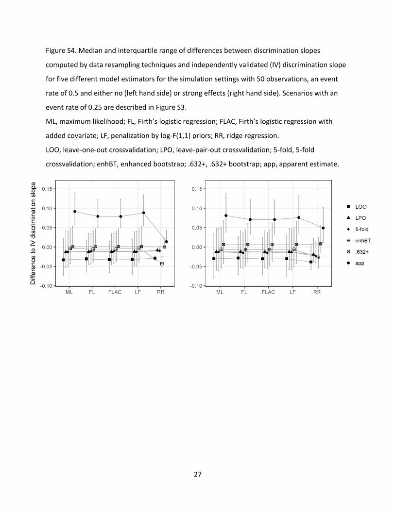
Figure S4. Median and interquartile range of differences between discrimination slopes

computed by data resampling techniques and independently validated (IV) discrimination slope

for five different model estimators for the simulation settings with 50 observations, an event

rate of 0.5 and either no (left hand side) or strong effects (right hand side). Scenarios with an

event rate of 0.25 are described in Figure S3.





28

Figure S5: Independently validated (solid line) and leave-one-out crossvalidated (dashed line) c

statistics for different penalization strengths in ridge regression on six artificially constructed

data sets. The data were created in the same way as for one of the scenarios in our simulation

study (null scenario, sample size of 50, marginal event rate of 0.25). The x-axis shows the tuning

parameter in ridge regression (lambda in the R package glmnet) with higher values

corresponding to stronger penalization. For each data set we fitted 96 ridge regression models

corresponding to a series of log-equidistant tuning values. As in our simulation study, the

independently validated c statistics were obtained by validating the models on an independent

data set consisting of 100,000 observations. As expected, the independently validated c

statistics are very close to the true value of 0.5.

LOO, leave-one-out crossvalidation; IV, independently validated.

c statistics and discrimination slopes: should leave one

Documents