J. Fluid Mech., page 1 of 14. c© Cambridge University Press 2012 1doi:10.1017/jfm.2011.558

C-start: optimal start of larval fish

M. Gazzola, W. M. Van Rees and P. Koumoutsakos†

Institute of Computational Science, ETH Zurich, Universitatsstrasse 6, CH-8092 Zurich, Switzerland

(Received 19 August 2011; revised 2 December 2011; accepted 19 December 2011)

We investigate the C-start escape response of larval fish by combining flow simulationsusing remeshed vortex methods with an evolutionary optimization. We test thehypothesis of the optimality of C-start of larval fish by simulations of larval-shaped,two- and three-dimensional self-propelled swimmers. We optimize for the distancetravelled by the swimmer during its initial bout, bounding the shape deformation basedon the larval mid-line curvature values observed experimentally. The best motionsidentified within these bounds are in good agreement with in vivo experiments andshow that C-starts do indeed maximize escape distances. Furthermore we found thatmotions with curvatures beyond the ones experimentally observed for larval fish mayresult in even larger escape distances. We analyse the flow field and find that theeffectiveness of the C-start escape relies on the ability of pronounced C-bent bodyconfigurations to trap and accelerate large volumes of fluid, which in turn correlateswith large accelerations of the swimmer.

Key words: propulsion, swimming/flying

1. IntroductionFish burst accelerations from rest are often observed in predator–prey encounters.

These motions may be distinguished into C- and S-starts, according to the bendingshape of the swimmer. Predators mainly exhibit S-starts during an attack, while C-starts are typical escaping mechanisms observed in prey (Domenici & Blake 1997).Since the first detailed report by Weihs (1973), C-start behaviour has attracted muchattention with studies considering the resulting hydrodynamics and the kinematics ofthese motions (Domenici & Blake 1997; Budick & O’Malley 2000; Muller & vanLeeuwen 2004; Muller, van den Boogaart & van Leeuwen 2008) in experiments(Tytell & Lauder 2002; Epps & Techet 2007; Muller et al. 2008; Conte et al. 2010)and simulations (Hu et al. 2004; Katumata, Muller & Liu 2009).

Several works have suggested that C-start is an optimal escape pattern (Howard1974; Weihs & Webb 1984; Walker et al. 2005), but to the best of our knowledge,this has been an observation and not the result of an optimization study. The goalof the present work is to perform an optimization of the fish motion, for a specifiedzebrafish-like geometry, maximizing the distance travelled over few tail beats by aswimmer starting from rest. The optimization couples the covariance matrix adaptationevolution strategy (Hansen, Muller & Koumoutsakos 2003) with two-dimensional and

† Email address for correspondence: petros@inf.ethz.ch

2 M. Gazzola, W. M. Van Rees and P. Koumoutsakos

S1 S3S2 S4 S5 S6

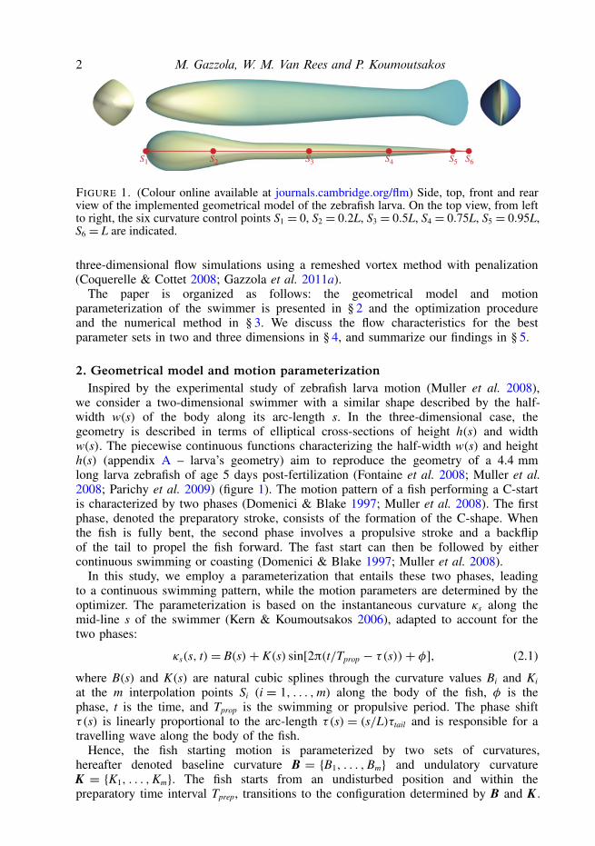
FIGURE 1. (Colour online available at journals.cambridge.org/flm) Side, top, front and rearview of the implemented geometrical model of the zebrafish larva. On the top view, from leftto right, the six curvature control points S1 = 0, S2 = 0.2L, S3 = 0.5L, S4 = 0.75L, S5 = 0.95L,S6 = L are indicated.

three-dimensional flow simulations using a remeshed vortex method with penalization(Coquerelle & Cottet 2008; Gazzola et al. 2011a).

The paper is organized as follows: the geometrical model and motionparameterization of the swimmer is presented in § 2 and the optimization procedureand the numerical method in § 3. We discuss the flow characteristics for the bestparameter sets in two and three dimensions in § 4, and summarize our findings in § 5.

2. Geometrical model and motion parameterizationInspired by the experimental study of zebrafish larva motion (Muller et al. 2008),

we consider a two-dimensional swimmer with a similar shape described by the half-width w(s) of the body along its arc-length s. In the three-dimensional case, thegeometry is described in terms of elliptical cross-sections of height h(s) and widthw(s). The piecewise continuous functions characterizing the half-width w(s) and heighth(s) (appendix A – larva’s geometry) aim to reproduce the geometry of a 4.4 mmlong larva zebrafish of age 5 days post-fertilization (Fontaine et al. 2008; Muller et al.2008; Parichy et al. 2009) (figure 1). The motion pattern of a fish performing a C-startis characterized by two phases (Domenici & Blake 1997; Muller et al. 2008). The firstphase, denoted the preparatory stroke, consists of the formation of the C-shape. Whenthe fish is fully bent, the second phase involves a propulsive stroke and a backflipof the tail to propel the fish forward. The fast start can then be followed by eithercontinuous swimming or coasting (Domenici & Blake 1997; Muller et al. 2008).

In this study, we employ a parameterization that entails these two phases, leadingto a continuous swimming pattern, while the motion parameters are determined by theoptimizer. The parameterization is based on the instantaneous curvature κs along themid-line s of the swimmer (Kern & Koumoutsakos 2006), adapted to account for thetwo phases:

κs(s, t)= B(s)+ K(s) sin[2π(t/Tprop − τ(s))+ φ], (2.1)

where B(s) and K(s) are natural cubic splines through the curvature values Bi and Ki

at the m interpolation points Si (i = 1, . . . ,m) along the body of the fish, φ is thephase, t is the time, and Tprop is the swimming or propulsive period. The phase shiftτ(s) is linearly proportional to the arc-length τ(s) = (s/L)τtail and is responsible for atravelling wave along the body of the fish.

Hence, the fish starting motion is parameterized by two sets of curvatures,hereafter denoted baseline curvature B = B1, . . . ,Bm and undulatory curvatureK = K1, . . . ,Km. The fish starts from an undisturbed position and within thepreparatory time interval Tprep, transitions to the configuration determined by B and K .

C-start: optimal start of larval fish 3

After this stage the preparatory stroke is completed and the fish transitions (withinTprop) to the propulsive configuration, completing its first swimming motion cycle.By the end of this cycle, at t = Tprep + Tprop, the baseline curvature has returned tozero, and another cycle follows which is solely determined by the curvature K . Eachtransition from one configuration to another is carried out through a cubic interpolationbetween start and end curvature (setting the first derivative at the extrema to zeroto ensure smoothness) within the prescribed time interval. The parameter τtail is alsoramped up via cubic interpolation from zero to its designated value at Tprep. We notethat the use of a baseline curvature B arises from the observation that the C-startmotion is not periodic, as it would be if only undulatory curvature K were to beconsidered. Therefore B enables the model to capture a broader range of deformations,thus enlarging the reproducible set of possible motions.

We use six control points located at S1 = 0, S2 = 0.2L, S3 = 0.5L, S4 = 0.75L,S5 = 0.95L, S6 = L (figure 1) and the curvature at S1, S2 and S6 is set to zero.These locations and curvature constraints are chosen to model the stiff head, theincreasing flexibility towards the posterior of the body and the stiff last fraction ofthe tail (Muller & van Leeuwen 2004; Fontaine et al. 2008; Muller et al. 2008).Furthermore, we fix the ratio between the preparatory and propulsive time intervalto Tprep/Tprop = 0.7, based on the experimental observations of Muller et al. (2008)and Budick & O’Malley (2000), and set Tprep + Tprop = 1 physical time unit. Duringthe optimization we reject cases where |κs(s, t)| > 2π/L. These curvature constraintsconform with the range of curvature values experimentally observed in fast starts oflarval zebrafish (Muller et al. 2008), even though they may not be directly related tolarval biomechanical properties.

In summary, the fish starting motion is characterized by eight free parameters,namely B3, B4, B5, K3, K4, K5, τtail , and φ, which will be varied during theoptimization. We emphasize that biomechanics is not considered in our model andflow-induced body deformations are not accounted for in this study.

3. Optimization of starting motionBased on extensive experimental observations, Domenici & Blake (1997)

emphasized that the quantities relevant to evaluating fast starts are distance or speedattained and the time interval of such responses. Therefore we chose to identify thestarting motion pattern (characterized by B, K , τtail , and φ) via the optimization ofthe maximum distance travelled by the centre of mass of the swimmer (dT

max) inthe time interval [0,T = Tprep + 2Tprop]. Within this interval, the fish performs thepreparatory stroke, the propulsive stroke and one additional swimming cycle. This timeinterval is chosen so as to capture the full start while also allowing examination of thefinal swimming pattern. The identification of the optimal parameter set is cast into aminimization problem where the cost function is defined as f =−|dT

max |.The optimization is performed using the covariance matrix adaptation evolutionary

strategy (CMA-ES) in its multi-host, rank-µ and weighted recombination form(Hansen et al. 2003; Gazzola, Vasilyev & Koumoutsakos 2011b). Evolution strategieshave been shown to be effective in dealing with computational and experimental,single and multi-objective, flow optimization problems (Buche et al. 2002; Kern &Koumoutsakos 2006; Gazzola et al. 2011b). The CMA-ES is an iterative algorithmthat operates by sampling, at each generation, p candidate parameter vectors from amultivariate Gaussian distribution N (m, σ 2C). Its mean m, overall standard deviationσ and covariance matrix C are adapted based on past successful parameter vectors,

4 M. Gazzola, W. M. Van Rees and P. Koumoutsakos

ranked according to their cost function values. We note that de-randomized evolutionstrategies do not ensure that the global optimum is found. In turn the robustnessof CMA-ES is mainly controlled by the population size p (Hansen et al. 2003).Here, as a tradeoff between robustness and fast convergence, we set p = 100 forthe two-dimensional case, while for the three-dimensional case, given the highercomputational costs, we reduced it to p = 40. The search space is bounded for allcurvature parameters by [−2π/L, 2π/L], and for τtail and φ by [0, 2π] (furthermore|κs(s, t)| 6 2π/L at all times and invalid configurations are discarded). Bounds areenforced during the sampling through a rejection algorithm. The initial parametervector was set to 0 for the two-dimensional case, while for the three-dimensional case,we started from the best parameter set found during the two-dimensional optimization.Initial standard deviations were set to 1/15 of the corresponding search spaceinterval.

3.1. Equations and numerical method

We consider a deforming and self-propelling body in a viscous incompressible flowdetermined by solving the incompressible Navier–Stokes equations:

∂u∂t+ (u ·∇)u=− 1

ρ∇p+ ν∇2u, x ∈Σ \Ω, (3.1)

where ρ is the fluid density (set equal to body density), ν the kinematic viscosity, Σthe computational domain and Ω the support of the body. The action of the bodyon the fluid is realized through the no-slip boundary condition at the interface ∂Ω ,enforcing the body velocity (us) to be the same as the fluid velocity (u). The feedbackfrom the fluid to the body is in turn described by Newton’s equation of motionmsxs = F and d(I sθ s)/dt = M , where xs, θ s, ms, I s, F and M are, respectively, thebody’s centre of mass, angular velocity, mass, moment of inertia and hydrodynamicforce and momentum exerted by the fluid on the body.

The flow is solved via a remeshed vortex method, characterized by a Lagrangianparticle advection, followed by particle remeshing and the use of an FFT-basedPoisson solver (Koumoutsakos & Leonard 1995; Koumoutsakos 1997). The remeshedvortex method was coupled to Brinkman penalization, a projection approach handlesthe feedback from the flow to the body, while the body surface is tracked implicitlyby a level set (Coquerelle & Cottet 2008). The penalization term added to theNavier–Stokes equations approximates the no-slip boundary condition at the bodyinterface, and allows the control on the solution error through the penalization factor λ.This algorithm has been extended to non-divergence-free deformations for single andmultiple bodies (Gazzola et al. 2011a).

Equation (3.1) is cast into its velocity (u)–vorticity (ω =∇ × u) formulation

∂ω

∂t+∇ · (u : ω)= (ω ·∇)u+ ν∇2ω + λ∇ × χs(us − u), x ∈Σ, (3.2)

where ∇ · (u : ω) is the vector with components ∂/∂xi(uiωj), χs the characteristicfunction (Gazzola et al. 2011a) describing the body shape and λ 1 the penalizationfactor (here λ = 104 and the mollification length of χs is ε = 2

√2h, h being the grid

spacing). Translational (uT) and rotational (uR) components of us = uT + uR + uDEF arerecovered through a projection approach. The deformation velocity uDEF (prescribed apriori) is specific to the shape under study. As uDEF is in general non-solenoidal, the

C-start: optimal start of larval fish 5

–1.6

–1.4

–1.2

–1.0

–0.8

–0.6

–0.4

–0.2C

ost f

unct

ion

(L–1

)

0 2000 4000

Evaluations Evaluations6000 8000 0 100 200 300 400 500 600

–1.25

–1.20

–1.15

–1.10

–1.05

–1.00(a) (b)

FIGURE 2. (Colour online) Cost function value f (normalized by L) against number ofevaluations: two-dimensional (a) and three-dimensional (b) optimizations. Solid (blue online)and dashed (green online) lines correspond to, respectively, best solution in the currentgeneration and best solution ever. The best two-dimensional solution was used as startingsearch point in the three-dimensional case.

B3 B4 B5 K3 K4 K5 τtail φ fBest two-dimensional −3.19 −0.74 −0.44 −5.73 −2.73 −1.09 0.74 1.11 −1.53Best three-dimensional −1.96 −0.46 −0.56 −6.17 −3.71 −1.09 0.65 0.83 −1.25

TABLE 1. Best motions identified through the optimization (curvatures normalized by L).

incompressibility constraint becomes ∇ · u = 0 for x ∈ Σ \ Ω and ∇ · u = ∇ · uDEF

for x ∈ Ω . This translates into recovering u from the Poisson equation ∇2u =−∇ × ω +∇(∇ ·uDEF), with unbounded boundary conditions (Gazzola et al. 2011a).

During the course of the optimization in two dimensions, simulations werecarried out in a domain [0, 4L] × [0, 4L], with constant resolution 1024 × 1024 andLagrangian CFL set to 0.1. Quantities of interest were recomputed at higher resolution(2048× 2048). In the three-dimensional case, simulations were carried out in a domainof variable size, growing in time to accommodate the wake. The grid spacing waskept constant at δx = L/256 during the optimization and at δx = L/512 for the higher-resolution runs that resulted in the reported diagnostics.

3.2. Flow conditions

We define the Reynolds number as Re = (L2/Tprop)/ν, where L is the fish length andTprop is the swimming period. Here we consider a body that models a zebrafish larvaof length L = 4.4 mm, corresponding to a fish of age 5 days post-fertilization (Mulleret al. 2008; Parichy et al. 2009). For a typical swimming period of Tprop ≈ 44 ms(Muller et al. 2008) in water, we obtain a Reynolds number Re = 550 and oursimulations were performed at this Reynolds number.

4. Results4.1. Two-dimensional swimmer

The course of the optimization for the two-dimensional swimmer is shown infigure 2(a) and the best parameter set is presented in table 1. This parameter setinduces the motion sequence illustrated in figures 3 and 4. The solution found closely

6 M. Gazzola, W. M. Van Rees and P. Koumoutsakos

FIGURE 3. (Colour online) Vorticity fields of the two-dimensional best solution (bluenegative and red positive vorticity) time sequence (0 6 t 6 2.35Tprop;1t = 0.156Tprop).

3D(a) (b) Exp. 2D 3D

Exp.

2D

10 ms 20 ms 30 ms 40 ms 50 ms

4

3

2

1

ms

Preparatory stroke

Propulsive stroke

FIGURE 4. (Colour online) Zebrafish larva C-start, experiments and simulations. (a) Vorticityfields (blue negative and red positive vorticity) and (b) swimming kinematics, represented bybody mid-lines, corresponding to the best two-dimensional (2D) and three-dimensional (3D)solutions found via the optimization procedure and experimental observations by Muller et al.(2008).

reproduces the starting bout observed experimentally in larval zebrafish (Muller et al.2008). During the preparatory stroke, the fish bends into a C-shape, then straightens topropel itself forward and completes its cycle.

In order to further quantify C-start mechanics and to elucidate its hydrodynamics,we considered, at time tA = Tprep + Tprop and tB = Tprep + 2Tprop, respectively, the first(A) and second (B) vortex pair generated by nine different motion patterns (figure 5).The reference motion pattern is defined by the best parameters as found by theoptimization process (case 0). We systematically increased/decreased the curvatureK2D

best and B2Dbest corresponding to the best solutions found (cases −3 to 4 as detailed

in figure 5) in order to assess the impact of the C-curvature on the flow. We notethat cases −3, −2, −1 lie outside the parameter search space of the optimization(since K3 > 2π/L). These cases are included in order to explore the effect of curvaturevalues beyond those reported experimentally. Furthermore, in case 5 we considered asreference a ‘slow start’ performed by anguilliform swimming, an archetypal mode oflocomotion characterized by the propagation of curvature waves from the anterior to

C-start: optimal start of larval fish 7

0 0.5 1.0 1.5 2.0 2.5

5

10

15

20

25

30

35

0

0.2

0.4

0.6

0.8Rat

io

1.0

1.2

1.4

1.6

–3 –2 –1 1

Case3 42 5 –3 –1–2 10

Case3 42 5

0

0.2

0.4

0.6

0.8

1.0

1.2

(b)

(c) (d)

0

Spee

d (L

s–1

)

A

B

(a)

FIGURE 5. (Colour online) Vortex pair characterization in the two-dimensional setup. Ninemotions are considered: the maximum found (case 0), motions with enhanced/reducedcurvature with respect to case 0 (130 %, 120 %, 110 %, 90 %, 80 %, 70 %, 60 %, respectively,case −3, −2, −1, 1, 2, 3, 4), and (case 5) cruise swimming. (a) First (A) and second(B) vortex pairs at time, respectively, tA = Tprep + Tprop and tB = Tprep + 2Tprop, for case0. (b) Speed of the fish centre of mass, from top to bottom, cases −3 to 5, expressed inlength/seconds, based on a zebrafish of L = 4.4 mm and Tprop ≈ 44 ms in water. (c) Vortexpairs’ (A, circle; B, diamond) relative total circulation (|Γ |/|Γ0|, black) and area (|A|/|A0|,red) with respect to case 0, versus all cases. Vortex cores in A/B, are localized via the criterion|ω| > 0.15 max |ω0|, where max |ω0| is the maximum vorticity of structure A/B in case 0. (d)Relative distance travelled (f /f0, black) and energetic efficiency (η/η0, red).

the posterior of the body. We used the kinematic description given in Gazzola et al.(2011a) along with a cubic interpolation to ramp up the motion within Tprep. As canbe seen in figure 5, areas and circulations |Γ | of the shed vortex pairs A and Bmonotonically decrease with reducing curvature magnitude, except for the area of thevortical structure B which shows a maximum for case −1. In case 5 the areas andcirculations, of structures A and B, are found to be substantially smaller than in allother cases. Figure 5(b) shows that the fish achieves larger speed on increasing thecurvature, indicating a correlation between the strength of vortex cores and speed.However, speed does not necessarily translate into a larger distance travelled bythe centre of mass, due to increased lateral velocities, as depicted in figure 5(d)where a maximum is observed for case −1 (∼1 % better than case 0). Therefore,the best solution found within the curvature range observed experimentally can befurther improved with increased curvature. Nevertheless, within the experimentallyobserved curvature values we found that C-starts are the best escape mechanisms.

8 M. Gazzola, W. M. Van Rees and P. Koumoutsakos

3D, case 0

3D, case 3

2D, case 0

2D, case 3

FIGURE 6. (Colour online) Particle tracking and F-FTLE time sequence (0.5Tprop 6 t 61.25Tprop;1t = 0.25Tprop). F-FTLE was computed given the integration time TLE = 1.59Tprop.

The figure also shows the efficiency η = (m/2) (τ−1∫τU dt)2/

∫τ

P dt (where m and Uare mass and velocity of the swimmer, P is the power imparted to the fluid andτ = Tprep + 2Tprop, see appendix B – definition of efficiency) of the start procedure. Weobserve that the efficiency peaks between cases 2 and 3, and that the anguilliform startoutperforms all C-starts. The plot also shows how C-starts are energetically inefficient,consistent with the observation that burst swimming modes are sustained for short timeintervals by fish.

We performed particle tracking for case 0 (figure 6), advecting backwards in timepassive particles initialized within vortical structure A, to qualitatively illustrate C-start dynamics. Particle locations are superimposed on a forward finite-time Lyapunovexponent (F-FTLE) field (Haller & Yuan 2000) to highlight regions of coherentflow behaviour. As can be noticed, particles are accelerated along the body, gainingmomentum and circulation before being shed into a vortex pair. The fluid regiontrapped inside the area bounded by the C-shape of the larva, surrounded by thetracked particles, is accelerated as well and ejected opposite to the swimming direction,without much vorticity being generated. Figure 6 pictures the same analysis also forcase 3, to illustrate how a smaller curvature corresponds to a smaller fluid regionbounded by the C-shape. We conclude that increasing C-curvature results in strongervortex pairs, which during their formation, due to transfer of momentum, contribute tothe swimmer’s acceleration, albeit at a decreased efficiency.

4.2. Three-dimensional swimmerThe evolution of the motion parameters for the three-dimensional case is shown infigure 2(b), and the best parameter set found is given in table 1. The most notabledifferences between the best parameters in three dimensions with respect to those intwo dimensions are the reduced values of B3 and B4, indicating a smaller curvatureof the posterior half of the fish during the preparatory stroke, and the increasedvalues of K3, K4 and K5, corresponding to larger curvatures during the propulsivestage. Compared to two dimensions, the complete motion in three dimensions differsin the continuous swimming phase, where the large curvature values of K3–K5 resultin larger deformations of the body (figure 7). The forward velocity of the best three-dimensional larval fish is slightly smaller than in two dimensions, and reaches amaximum of 14 L s−1 during the propulsive stroke and 23 L s−1 during the ensuingswimming motion. Experimentally reported values for this fish at a similar Reynolds

C-start: optimal start of larval fish 9

(a) (b)

FIGURE 7. (Colour online) (a) Vorticity fields of the three-dimensional best solution foundduring the optimization (blue negative and red positive z-component of ω) time sequenceat times t/Tprop 0.13, 0.43, 0.71, 1.04, 1.61 and 2.15 (left to right, top to bottom).Supplementary movie available at http://dx.doi.org/10.1017/jfm.2011.558. (b) Evolution ofpassive tracer particles seeded at t/Tprop = 0.5 and overlaid on the ωz-field. Three sets ofparticles (dark–medium–light grey-scale) are initialized in different regions of the F-FTLEfield. Sequence times as in figure 6.

number are 7 L s−1 for the propulsive stroke and swimming velocities between14 L s−1 and 24 L s−1 (Muller et al. 2008). We observe that the simulated fish speedsare higher than those reported experimentally for the propulsive stroke while the speedof swimming motion is in good agreement with the experimental results.

The three-dimensional flow visualizations show that during the preparatory stroke,the larva tail generates a starting vortex ring travelling towards the swimmer’s head.The formation of this vortex ring is not accompanied by significant accelerationof the body. During the first backflip of the tail (the propulsive stroke), the fishcontinuously generates vorticity along the complete profile of the tail. The resultingvortical structure is a vortex ring elongated along its top and bottom halves (figure 7),indicating a stronger vorticity generation at the top and bottom of the tail thanat the middle as justified by the tail geometry. The vortical structures generatedin subsequent swimming strokes are similar to this elongated vortex ring. Theflow structures of the two-dimensional simulations and the mid-plane of the three-dimensional simulations are visually consistent with the experimental results reportedin Muller et al. (2008) (figure 4). We remark that the elongated vortex rings that canbe observed in the experimental results during the propulsive phase are also observedin the vorticity field of the three-dimensional simulations.

We have performed for the three-dimensional simulations a similar analysis as forthe two-dimensional case by considering the vorticity field in the horizontal mid-plane,passing through the centre of mass of the fish (figure 8). We note similar trends for thecirculation and area of the vortical structures A and B and fish speed. Also efficiencyand distance travelled show a comparable behaviour between the two-dimensionaland three-dimensional simulations, except for a larger difference in distance travelledbetween cases −1 and 0 (∼4.5 %). The particle tracking was performed for thethree-dimensional simulation by placing the particles on the first vortex pair in themid-plane of the swimmer (figure 6) and tracing the particles back in time. Theparticles stay on the mid-plane due to the vertical symmetry in the flow. However,contrary to the two-dimensional case, only few of the particles trace back to the

10 M. Gazzola, W. M. Van Rees and P. Koumoutsakos

0

5

10

15

20

25

30

0.5 1.0 1.5 2.0 2.5

(a)

(c) (d)

(b)

0

0.2

0.4

0.6

0.8

1.0

1.2

1.4

Rat

io

–3 –2 –1 1

Case3 42 50

0

0.2

0.4

0.6

0.8

1.0

1.2

1.4

–3 –2 –1 1

Case3 42 50

Spee

d (L

s–1

)

A

B

FIGURE 8. (Colour online) As figure 5 but for vortex ring characterization in thethree-dimensional setup.

region bounded by the C-shape of the swimmer. A forward particle tracking was thenperformed to determine the path of the particles originating in the C-shape region(figure 7). The time frames show that the particles spread over a wide region behindthe fish, bounded on two sides by a region of vorticity. This indicates that also in thethree-dimensional case the fish accelerates a large region of fluid originating withinthe C-shape of the swimmer but the accelerated fluid spreads out over a much widerregion than in the two-dimensional case.

5. ConclusionsWe have performed a reverse engineering study of larval starting motions to identify

the patterns which maximize the escape distance, coupling an evolution strategy withtwo- and three-dimensional flow simulations. The geometrical model, time scales andparameter search space were dictated by experimental observations of larval fish. Theidentified best motion kinematics are in good agreement with in vivo observationsand exhibit C-start patterns, indicating that C-starts do indeed maximize the escapedistance. The flow field is characterized by elongated vortex rings stretched bythe zebrafish tail. The forward swimming velocities obtained in three-dimensionalsimulations are in good agreement with those measured in experiments while thevortical structures observed in the mid-plane are consistent with those reported inexperiments (Muller et al. 2008). We find that the effectiveness of the C-start escape

C-start: optimal start of larval fish 11

relies on the ability of pronounced C-bent configurations to trap and accelerate largeamounts of fluid. Furthermore C-starts are found to be energetically inefficient. Aparametric investigation around our best solutions indicates that increasing curvaturesbeyond experimentally based bounds can lead to even larger escape distances. Futurework will further investigate this latter observation and the multi-objective optimizationof motion patterns using multi-resolution flow simulations.

Supplementary movies are available at http://dx.doi.org/10.1017/jfm.2011.558.

Appendix A. Larva’s geometryThe geometrical aspect of the swimmer is characterized by the half width w(s) of

the body along its length, defined as:

w(s)=

wh

√1−

(sb − s

sb

)2

0 6 s< sb

(−2(wt − wh)− wt(st − sb))

(s− sb

st − sb

)3

+

(3(wt − wh)+ wt(st − sb))

(s− sb

st − sb

)2

+ wh sb 6 s< st

wt − wt

(s− st

L− st

)2

st 6 s 6 L

(A 1)

where L is the body length, sb = 0.0862L, st = 0.3448L, wh = 0.0635L and wt =0.0254L. In the three-dimensional case, the geometry is described in terms of ellipticalcross sections with width w(s) and height h(s), where h(s) is given by

h(s)=

h1

√1− (s− s1)

2

s21

0 6 s 6 s1

−2(h2 − h1)

(s− s1

s2 − s1

)3

+ 3(h2 − h1)

(s− s1

s2 − s1

)2

+ h1 s1 < s 6 s2

−2(h3 − h2)

(s− s2

s3 − s2

)3

+ 3(h3 − h2)

(s− s2

s3 − s2

)2

+ h2 s2 < s 6 s3

h3

√1−

(s− s3

L− s3

)2

s3 < s 6 L.

(A 2)

Here we use the following parameter pairs: (s1, h1) = (0.284L, 0.072L), (s2, h2) =(0.844L, 0.041L) and (s3, h3)= (0.957L, 0.071L).

Appendix B. Definition of efficiencyWe define the efficiency as follows:

η = Euseful

Eflow, (B 1)

where Euseful is the kinetic energy of the fish:

Euseful = 12

mU2, (B 2)

12 M. Gazzola, W. M. Van Rees and P. Koumoutsakos

with U the mean velocity of the fish during the simulation time (Tprep + 2Tprop) and mthe fish mass.

The term Eflow represents the total energy delivered to the fluid,

∫ Tprep+2Tprop

τ=0Pflow(t) dτ, (B 3)

where Pflow is the total instantaneous power delivered to the fluid, which accounts forrate of change of kinetic energy and dissipation due to viscous stresses:

Pflow = d

dt

∫Ωf

ρu2

2dΩ + µ

∫Ωf

(∇u+ (∇u)T) :∇u dΩ, (B 4)

with Ωf denoting the spatial region occupied with fluid, and u2 = u · u.Since we have a computational domain with free-space boundary conditions, the

velocity field is not completely contained within the computational domain and theevaluation of the above integrals is not trivial. We will discuss the contribution of thevelocity field outside our computational domain for each of the two terms in the righthand side of (B 4).

For the first term we first note that, for a divergence-free velocity field, thefollowing kinematic identity holds Winckelmans & Leonard (1993):∫

Ω

u · u dΩ =∫Ω

Ψ · ω dΩ. (B 5)

Here Ψ is the streamfunction, defined as the solution of the Poisson equation

∇2Ψ =−ω, (B 6)

hence u = ∇ × Ψ . The integral on the right-hand side can be computed in Fourierspace from a compact vorticity field, and thus the kinetic energy in a domain withfree-space boundary conditions can be computed as a function of the vorticity fieldonly. To get the kinetic energy in the fluid domain only, we subsequently subtract thekinetic energy within the fish from this sum. Finally, the time derivative of the integralis computed as a first order finite difference between two timesteps.

In the current case, however, the velocity field inside the swimmer is not divergencefree (due to the deformation velocity field of the swimmer – for more details refer toGazzola et al. (2011a)). The integral in (B 5) therefore is an incomplete measure ofthe total kinetic energy since it neglects the contribution of the potential to the velocityfield. After initial tests comparing the influence of the potential, however, we observedthat this contribution to both the total kinetic energy as well as its time-derivative wasseveral orders of magnitude smaller than the contribution from the stream function. Tosave in computational costs we therefore chose to neglect the contribution from thepotential and base the efficiency on the kinetic energy due to the vorticity-inducedvelocity only.

The second integral in (B 4) represents the viscous dissipation term. Bysystematically increasing the domain size, we found that the contribution this increase

C-start: optimal start of larval fish 13

is negligible and we therefore compute this integral only inside the computationaldomain.

R E F E R E N C E S

BUCHE, D., STOLL, P., DORNBERGER, R. & KOUMOUTSAKOS, P. 2002 Multiobjective evolutionaryalgorithm for the optimization of noisy combustion processes. IEEE Trans. Syst. Man Cybern.C 32 (4), 460–473.

BUDICK, S. A. & O’MALLEY, D. M. 2000 Locomotor repertoire of the larval zebrafish: swimming,turning and prey capture. J. Expl Biol. 203 (17), 2565–2579.

CONTE, J., MODARRES-SADEGHI, Y., WATTS, M. N., HOVER, F. S. & TRIANTAFYLLOU, M. S.2010 A fast-starting mechanical fish that accelerates at 40 m s(−2). Bioinspir. Biomim. 5 (3).

COQUERELLE, M. & COTTET, G. H. 2008 A vortex level set method for the two-way coupling ofan incompressible fluid with colliding rigid bodies. J. Comput. Phys. 227 (21), 9121–9137.

DOMENICI, P. & BLAKE, R. W. 1997 The kinematics and performance of fish fast-start swimming.J. Expl Biol. 200 (8), 1165–1178.

EPPS, B. P. & TECHET, A. H. 2007 Impulse generated during unsteady maneuvering of swimmingfish. Exp. Fluids 43 (5), 691–700.

FONTAINE, E., LENTINK, D., KRANENBARG, S., MULLER, U. K., VAN LEEUWEN, J. L., BARR,A. H. & BURDICK, J. W. 2008 Automated visual tracking for studying the ontogeny ofzebrafish swimming. J. Expl Biol. 211 (8), 1305–1316.

GAZZOLA, M., CHATELAIN, P., VAN REES, W. M. & KOUMOUTSAKOS, P. 2011a Simulations ofsingle and multiple swimmers with non-divergence free deforming geometries. J. Comput.Phys. 230 (19), 7093–7114.

GAZZOLA, M., VASILYEV, O. V. & KOUMOUTSAKOS, P. 2011b Shape optimization for dragreduction in linked bodies using evolution strategies. Comput. Struct. 89 (11–12), 1224–1231.

HALLER, G. & YUAN, G. 2000 Lagrangian coherent structures and mixing in two-dimensionalturbulence. Physica D 147 (3–4), 352–370.

HANSEN, N., MULLER, S. D. & KOUMOUTSAKOS, P. 2003 Reducing the time complexity of thederandomized evolution strategy with covariance matrix adaptation (cma-es). EvolutionaryComputation 11 (1), 1–18.

HOWARD, C. H. 1974 Optimal strategies for predator avoidance: the relative importance of speedand manoeuvrability. J. Theor. Biol. 47 (2), 333–350.

HU, W. R., YU, Y. L., TONG, B. G. & LIU, H. 2004 A numerical and analytical study on atail-flapping model for fish fast c-start. Acta Mechanica Sin. 20 (1), 16–23.

KATUMATA, Y., MULLER, U. K. & LIU, H. 2009 Computation of self-propelled swimming in larvafishes. J. Biomech. Sci. Engng 4 (1), 54–66.

KERN, S. & KOUMOUTSAKOS, P. 2006 Simulations of optimized anguilliform swimming. J. ExplBiol. 209 (24), 4841–4857.

KOUMOUTSAKOS, P. 1997 Inviscid axisymmetrization of an elliptical vortex. J. Comput. Phys. 138(2), 821–857.

KOUMOUTSAKOS, P. & LEONARD, A. 1995 High-resolution simulations of the flow around animpulsively started cylinder using vortex methods. J. Fluid Mech. 296, 1–38.

MULLER, U. K., VAN DEN BOOGAART, J. G. M. & VAN LEEUWEN, J. L. 2008 Flow patterns oflarval fish: undulatory swimming in the intermediate flow regime. J. Expl Biol. 211 (2),196–205.

MULLER, U. K. & VAN LEEUWEN, J. L. 2004 Swimming of larval zebrafish: ontogeny of bodywaves and implications for locomotory development. J. Expl Biol. 207 (5), 853–868.

PARICHY, D. M., ELIZONDO, M. R., MILLS, M. G., GORDON, T. N. & ENGESZER, R. E. 2009Normal table of postembryonic zebrafish development: staging by externally visible anatomyof the living fish. Dev. Dyn. 238 (12), 2975–3015.

TYTELL, E. D. & LAUDER, G. V. 2002 The c-start escape response of polypterus senegalus:bilateral muscle activity and variation during stage 1 and 2. J. Expl Biol. 205 (17),2591–2603.

14 M. Gazzola, W. M. Van Rees and P. Koumoutsakos

WALKER, J. A., GHALAMBOR, C. K., GRISET, O. L., MCKENNEY, D. & REZNICK, D. N. 2005Do faster starts increase the probability of evading predators? Funct. Ecol. 19 (5), 808–815.

WEIHS, D. 1973 The mechanism of rapid starting of slender fish. Biorheology 10, 343–350.WEIHS, D. & WEBB, P. W. 1984 Optimal avoidance and evasion tactics in predator–prey

interactions. J. Theor. Biol. 106 (2), 189–206.WINCKELMANS, G. S. & LEONARD, A. 1993 Contributions to vortex particle methods for the

computation of three-dimensional incompressible unsteady flows. J. Comput. Phys. 109,247–273.