1

Comparison of Different Global Information Sources Used in Surface Radiative Flux Calculation: Radiative Properties of the Surface

Yuanchong ZhangAPAM, Columbia University at NASA GISSWilliam B. RossowNASA Goddard Institute for Space Studies

Paul W. Stackhouse Jr.NASA Langley Research Center

June 2006(Revised for submission to Journal of Geophysical Research)

https://ntrs.nasa.gov/search.jsp?R=20080006500 2019-02-07T05:59:34+00:00Z

2

ABSTRACTDirect estimates of surface radiative fluxes that resolve regional and weather-scale variabilityover the whole globe with reasonable accuracy have only become possible with the advent ofextensive global, mostly satellite, datasets within the past couple of decades. The accuracy of thesefluxes, estimated to be about 10-15 W/m2, is largely limited by the accuracy of the input datasets.The leading uncertainties in the surface fluxes are no longer predominantly induced by clouds butare now as much associated with uncertainties in the surface and near-surface atmosphericproperties. This study presents a fuller, more quantitative evaluation of the uncertainties for thesurface albedo and emissivity and surface skin temperatures by comparing the main available globaldatasets from the Moderate-Resolution Imaging Spectroradiometer product, the NASA GlobalEnergy and Water Cycle Experiment Surface Radiation Budget project, the European Centre forMedium-Range Weather Forecasts, the National Aeronautics and Space Administration, theNational Centers for Environmental Prediction, the International Satellite Cloud Climatology Project(ISCCP), the Laboratoire de Météorologie Dynamique, NOAA/NASA Pathfinder Advanced VeryHigh Resolution Radiometer project, NOAA Optimum Interpolation Sea Surface TemperatureAnalysis and the Tropical Rainfall Measuring Mission (TRMM) Microwave Image project. Thedatasets are, in practice, treated as an ensemble of realizations of the actual climate such that theirdifferences represent an estimate of the uncertainty in their measurements because we do not possessglobal “truth” datasets for these quantities. The results are globally representative and may be takenas a generalization of our previous ISCCP-based uncertainty estimates for the input datasets. Surface properties have the primary role in determining the surface upward shortwave (SW)and longwave (LW) flux. From this study, the following conclusions are obtained. Although land

3

surface albedos in the near-infrared remain poorly constrained (highly uncertain), they do not causetoo much error in total surface SW fluxes; the more subtle regional and seasonal variationsassociated with vegetation and snow are still in doubt. The uncertainty of the broadband black-skySW albedo for land surface from this study is about 7%, which can easily induce 5-10 W/m2uncertainty in (upwelling) surface SW flux estimates. Even though available surface (broadband)LW emissivity datasets differ significantly (3% - 5% uncertainty), this disagreement is confined towavelengths > 20 !m so that there is little practical effect (1-3 W/m2) on the surface upwelling LWfluxes. The surface skin temperature is one of two leading factors that cause problems with surfaceLW fluxes. Even though the differences among the various datasets are generally only 2-4 K, thiscan easily cause 10-15 W/m2 uncertainty in calculated surface (upwelling) LW fluxes.Significant improvements could be obtained for surface LW flux calculations by improvingthe retrievals of (in order of decreasing importance): (1) surface skin temperature, (2) surface air andnear-surface-layer temperature, (3) column precipitable water amount and (4) broadband emissivity.And for surface SW fluxes, improvements could be obtained (excluding improved cloud treatment)by improving the retrievals of (1) aerosols (from our sensitivity studies but not discussed in thiswork), and (2) surface (black-sky) albedo, of which, NIR part of the spectrum has much largeruncertainty.

4

1. IntroductionAnalyses of global satellite products have resulted in the production of several extensive anddetailed surface radiative flux datasets [Rossow and Lacis, 1990; Darnell and Staylor, 1992;Whitlock et al., 1995; Rossow and Zhang, 1995; Stackhouse et al., 2004; Zhang et al., 2004].However, the usefulness of these flux products for monitoring long-term variations of globalradiation budgets and climate changes, as well as in other applications such as biological andoceanic modeling, is dependent on two separate issues: (A) the current uncertainty (or reliability)that can be estimated by evaluation of the calculated radiative fluxes against more directmeasurements and (B) how much and by what means may the flux products be improved. To address(A), Zhang et al., [1995 and 2004] have compared their flux products against surface (and the topof atmosphere) flux observations to estimate their uncertainty. Their 2004 estimate is about 10-15W/m2 uncertainty for surface fluxes. For (B), they have conducted all the important sensitivitystudies by varying the input datasets (and the radiative transfer model parameters) to providequantitative uncertainty estimates of the impacts of realistically-assumed uncertainties of the inputdatasets. The “realistically-assumed” uncertainties for the input datasets were based on earlierestimates, mainly from the International Satellite Cloud Climatology Project (ISCCP) D1 [Rossowand Schiffer 1991]. Some of their conclusions are summarized here. (1) Although clouds have, fora long time, been highlighted as the major source of uncertainty in both planetary and surfaceradiation budgets, the advent of extensive cloud datasets has reduced this source of uncertainty. (2)As a result, other uncertainty sources have now become relatively more important and comparableto the uncertainty from cloud datasets. (3) For surface radiative flux estimates in particular, theaccuracy is now largely limited by two aspects of Earth observations that have long been assumed

5

to be adequately observed, especially during the satellite era, namely, the near-surface atmosphericradiative properties (temperature and humidity) that are usually obtained from atmospheric profilinginstruments and the surface radiative properties (surface skin temperature, solar albedo and infraredemissivity).Zhang et al. [2006] have presented a fuller, more quantitative evaluation of the uncertaintiesfor the near-surface air temperature and humidity by comparing the main available global datasetsthat are treated as an ensemble of realizations of the actual climate such that their differencesrepresent an estimate of the uncertainty in their values. Here we follow the same methodology tomake such comparisons for the surface properties (Section 2). In Section 3 we briefly summarizethe uncertainties of the surface radiation budget induced by the uncertainties of these input datasetsand discuss some implications for understanding and modeling the surface-atmosphere interactions.

2. Surface Radiative PropertiesThe five major global datasets (three from reanalysis and two from satellite-retrieval), usedin the comparison for near-surface atmospheric properties in our companion paper [Zhang et al.2006], also supply other parameters such as surface skin temperature and surface albedo, which areto be compared in this work (with some additional datasets). They are, (1) the first version of theECMWF reanalysis for a 15-year period (1979-1993, called ERA15 or ER in our figures/tables)[Gibson et al., 1999], (2) the first version of the NASA Data Assimilation Office (DAO) GoddardEarth Observing System (GEOS) reanalysis for a 15-year period (March 1980 to February1995,called GEOS-1 or GE in our figures/tables) [Takacs, et al., 1994], and (3) the second version of the

6

National Centers for Environmental Prediction reanalysis for a 51-year period (1948-1998, calledNCEP or NC in our figures/tables) [Kistler et al., 2001], (4) a version of TOVS from theInternational Satellite Cloud Climatology Project (ISCCP, thereafter ISCCP-TOVS) [Rossow et al.,1996] that is combined with the modified surface skin and air temperature from ISCCP-FD [Zhanget al., 2004], called ISCCP-FD-TOVS, shortened as FDTV (called TV in some figures/tables, and(5) 3I dataset from the Laboratoire de Météorologie Dynamique (LMD) group, who has developeda new analysis that produced temperature and humidity profiles dataset from TOVS (Path B)[consisting of the High resolution Infrared Radiation Sounder (HIRS), the Microwave Sounding Unit(MSU) and the Stratospheric Sounding Unit (SSU)] based on Improved Initialization Inversion(therefore, 3I) retrieval algorithm [see Scott et al., 1999]. For more details of these five datasets, seeZhang et al., [2006]. To simplify the presentation, unless otherwise indicated, we restrict thecomparisons to monthly means and, if available, monthly-hourly means for every sixth hour (UTC= 0h, 6h, 12h and 18h), for January, April, July and October of 1992. Except for some long-termvariations in the character of these datasets that we note below, this year is taken to be typical ofthese products. 2.1. Albedo The surface albedo, as defined by the ratio of the reflected to incident flux density at surfaceand reported from measurements or calculations, is usually the apparent albedo that is governed bythe radiative interactions between atmospheric multiple scattering and absorption and surfacereflection and absorption under specific atmospheric conditions (including clouds) and is also solar-zenith-angle dependent. As a result, it is highly variable in time because of the rapid variation of

7

atmospheric conditions and the slower variations of surface conditions. For theoretical and practicaluses, particularly in radiation modeling that can account for multiple scattering, there has long beenused the physical concept of a surface albedo without atmospheric (including clouds) effects.Though, this quantity is sometimes referred to “surface albedo” without clarification by manyauthors, a number of authors have actually distinguished it from the apparent albedo by usingdifferent names, e.g., “black-sky albedo” (BSA, as chosen in this study) [Jin et al., 2003b], “truealbedo” [Henderson-Sellers and Wilson, 1983], and “inherent albedo” [Liang et al., 1999]. Thus,BSA is the intrinsic property of the surface material (but still varies with solar zenith angle),independent of the properties of any overlying layer (atmosphere). Confusion arises when peopleuse the word “albedo” and neglect the difference between the apparent and black-sky albedo.Henderson-Sellers and Wilson [1983] actually pointed out: “Atmospheric scatter tends to increaseobserved clear-sky system albedo compared with true surface albedo.” Sometimes, people justsimply and approximately take “clear-sky albedo” (which is a special case of the apparent albedo,but still is very sensitive to the aerosol loading and humidity profile in the atmosphere) as BSA.Note BSA is the apparent albedo for the moon’s surface or for other no-atmosphere planets. Toderive surface BSA from actual measurements on the Earth, the measured (apparent) albedo valuesmust be “corrected” to eliminate all atmospheric multiple scattering and absorbing effects, includingshifts of the spectrum of illumination and the contribution from multiply-scattered radiation. BSAis widely used because it is BSA that is specified in a radiative transfer model for calculatingshortwave (SW) fluxes. In the following text, we use “albedo” alone when it is for general purposes,meaning that it can be any one of the different albedos or when the precise meaning is not known,while we use BSA or clear-sky albedo in a precise way. Similarly, the longwave (LW, terrestrial

8

radiation wavelengths) surface emissivity can be determined with or without atmospheric effects(no-atmosphere or “black-sky emissivity”, section 2.2).A. DatasetsSince the advent of satellites, various global, broadband, land surface albedo products havebeen derived either from satellite measurements alone [e.g., Staylor and Wilber, 1990, and Li andGarand, 1994, both from the Earth Radiation Budget Experiment (ERBE); Jin, et al., 2003b, fromthe Moderate-Resolution Imaging Spectroradiometer (MODIS)], or from a combination of thesurface spectral reflectivity properties for different surface types, compiled from surface, airborne,satellite and laboratory measurements, and classification of each location by vegetation-soil types[e.g., Csiszar and Gutman, 1999; Zhang et al., 1995]. The latter approach is used in virtually allweather forecast and climate models. Both methods (or some combination) are used by variousauthors in their calculations of surface and/or the top of the atmosphere (TOA) SW fluxes [e.g.,Rossow and Lacis, 1990; Darnell and Staylor, 1992; Pinker and Laszlo, 1992; Whitlock, et al., 1995;Zhang et al., 1995; Chen and Roeckner, 1996; Gupta, et al., 2001; Zhang et al., 2004].ERA15 used an albedo map [Gibson, et al., 1999] determined from a background yearlyclimatology with fixed values of 0.55 for sea ice and 0.07 for open water. For land the albedo variesbetween 0.07 and 0.80 whenever snow occurs but the albedo for snow-free vegetation is constantall year long, based on surface vegetation classification. GEOS-1 specifies its surface albedos fromPosey and Clapp [1964] with some modifications for land and fixed values of 0.07 and 0.80 for openwater and sea ice, respectively. For snow cover, albedo is usually greater than 0.4 [Takacs, et al.,1994]. The NCEP surface albedo comes from a climatology [Kanamitsu, 1989; Kalnay, 1996]: the

9

current land albedo is from Matthews [1985] with modification if there is snow cover (0.75 isassumed poleward of 70° latitude for permanent snow and 0.60 is assumed equatorward of 70° ifsnow depth is at least 0.01 m), sea ice albedo ranges from 0.45 - 0.65 and 0.65 - 0.8 for snow-freeand snow-covered, respectively, and open water albedo is solar-zenith-angle dependent but nospecifics could be found. NCEP albedos do not depend on the spectral interval (seeftp://ftpprd.ncep.noaa.gov/pub/cpc/wd51we/reanal/random_notes/model). Since all of the abovealbedo models are relatively simple, we do not use them for this work.The NASA Global Energy and Water Cycle Experiment (GEWEX) Surface RadiationBudget (SRB) Project has developed a 12-year/148-month global dataset for surface SW and LWfluxes on 1° X 1° grid, called SRB release 2 [Stackhouse et al., 2001, 2004] (now extended to 22yrs). The SW algorithm used for SRB is from Pinker and Laszlo [1992] in which land and oceanalbedo values, as a function of solar zenith angle and wavelength, are clear-sky surface albedosbased on Briegleb et al. [1986]. We call this version of albedo SRB-ALB.The NASA Goddard Institute for Space Studies (GISS) GCM Model II [Hansen, et al., 1983]uses a global, seasonally varying land surface albedo dataset that was constructed by combining aland surface type/vegetation classification from the work of Matthews [see Matthews, 1985] withfield and laboratory albedo measurements for different rock, soil and vegetation types. Snow istreated as an added component that modifies the surface albedo accordingly. Both snow and icealbedos are also (implicitly) solar-zenith-angle dependent. The spectrally and solar-zenith-angledependent ocean albedo is based on calculation of Fresnel reflection from a surface wave-slopedistribution as a function of wind speed [Cox and Munk, 1956]. The 1983-version of the albedovalues are for two wavelength ranges: visible (VIS) from 0.2 to 0.7 !m and near-infrared (NIR) from

10

0.7 to 5.0 !m, together covering the whole solar spectrum. The revised 2001 (current) version of thisproduct, which we will call GCM-ALB, has albedo values for six wavelength ranges: VIS and fivecovering the NIR. The revised ocean albedo includes the effects of foam and hydrosols. For all ofthe work using the GISS model, the default wind speed = 2 m/s [for a more detailed description, seeZhang et al., 2004]. The version used here for albedo values has a spatial resolution of 280 km andis “climatological” in that it represents no particular year (except for snow/ice areas).Based on the 1983 version of the GISS GCM, Zhang et al. [1995] produced a broadbandalbedo product by combining the surface visible albedo taken directly from visible reflectances (atwavelength about 0.6 !m) in the ISCCP cloud products [Rossow and Garder, 1993] and the GCM’sratio of the NIR to visible albedo. The land-type-dependent visible albedo is replaced by a 3-yearseasonal average of the ISCCP-C1 visible reflectances and the NIR albedos adjusted by regressionwith ERBE’s TOA clear-sky SW fluxes to minimize systematic errors. This product has a spatialresolution of 280 km and represents albedo values for particular time periods (1985 - 1988). Werefer to this dataset as ISCCP2-ALB (where the “2" refers to the number of spectral bands).Similarly, we have produced a updated version of the previous product by employing the 5spectral ratios of the 5 NIR wavelengths to visible albedo from the 2001 GISS GCM and the newISCCP-D1 surface visible reflectances (now corrected for aerosols using a climatology). We referto this dataset as ISCCP6-ALB, which is used in our new radiative transfer flux product ISCCP-FD[Zhang et al., 2004].The MODIS team (of Boston University) has produced a land surface albedo dataset atseveral spatial resolutions (from 5 km) for 16-day periods since February 2000 based on a three-parameter semi-empirical RossThick-LiSparse-Reciprocal (RTLSR) bidirectional reflectance

11

distribution function (BRDF) model to characterize the anisotropic reflectivity of the land surface[Jin et al., 2003a and b]. In their albedo retrieval irradiance model (MODTRAN), twenty surfacereflectance spectra, four visibility values for different aerosol loadings, five default aerosol models,twelve different water vapor profiles from the Tropical Ocean Global Atmosphere Coupled Ocean-Atmosphere Response Experiment project but with adjustments, and five types of default clouds(essentially some climatological atmosphere) are used [Liang et al., 1999]. The snow/ice flag isturned on if the majority of observations are indicated as snow/ice during a 16 day period, and onlythose observations are used for BRDF and albedo snow inversion [Schaaf et al., 2002]. The surfacecover types are assumed Lambertian. In this study, we use a dataset provided by Crystal B. Schaafat http://duckwater.bu.edu/brdf_albedo/albedo16/params.htm from the original version 4 product(MOD43C2 V004 16-day L3 Global 0.05° CMG, as of 2004). The original BRDF parameters for0.05° X 0.05° cells are used to calculate BSA for three wavelength ranges: visible (0.3-0.7 !m), NIR(0.7-5.0 !m) and total SW (0.3-5.0 !m) using a polynomial function of solar zenith angle (suppliedby MODIS team, see Lucht et al., [2000]) with a 16-day-mean solar zenith angle (representing a 16-day period “mean” BSA). The fine-scale albedo values are then (linearly) averaged to our standard280-km equal-area-map grid cells when ! 90% of the 0.05° cells have values within a box. Thisalbedo dataset, called MODIS-ALB, is for land only. Using the formulae provided by the MODISteam, we have produced MODIS BSA for four 16-day periods (beginning dates are 6 April, 11 Julyand 29 September 2000, and 17 January 2001) for comparison with matched values from ISCCP6-ALB for visible, NIR and total SW BSA, respectively. In addition, the MODIS BRDF parametersfor one 16-day period (11-24 July 2000, representing all of July) and two 16-day periods (1 Januaryto 1 February 2001) are used to calculate 3-hourly surface visible and NIR BSA values for these two

12

months that are then used in our current radiation model [Zhang et al., 2004] in place of ISCCP6-ALB to calculate ISCCP-FD-like MODIS (thereafter, MODIS-FD) 3-hourly TOA/surface clear-skyalbedoes/fluxes for July 2000 and January 2001. The monthly means are compared with matchingvalues from ISCCP-FD and the Clouds and the Earth’s Radiant Energy System (CERES) ERBE-likedatasets [Wielicki et al., 1996; see also Zhang et al., 2004].There are also various regional albedo products, e.g., the Meterosat Surface Albedo basedon two adjacent geostationary satellites Meteosat-7 and 5 (currently operated by EUMETSAT). Theproduction relies on a daily accumulation of the satellite observations acquired under more thanfifteen different illumination conditions to assess the scattering properties of the surface and theatmosphere with some assumptions, and estimates the directional hemispherical reflectance values,for visible band (~ 0.5-0.9) that is corrected for atmospheric effects (i.e., BSA), which may belinearly related to broadband albedo. The product is planned for retrievals of albedo values for thewhole Meteosat record (1982 to current) on a daily basis [Govaerts et al., 2004]. B. Comparison of Broadband Albedos Table 1a shows the global mean (rms = rms with bias removed, this will be used for all rmsvalues throughout the paper) of regional differences for monthly-mean clear-sky surface albedobetween ISCCP6-ALB and SRB-ALB for January, April, July and October, 1992 for four broadsurface types: snow-free land, ice-free water, snow-covered land and sea ice, where snow/ice cellsare defined by coverage !95% of a 280-km equal-area box on all the days of a month based on theISCCP snow/ice data. The last row of the table summarizes the average results for the four seasonalmonths. In general, the two albedo sets are in good agreement for snow-free land and ice-free water:

13

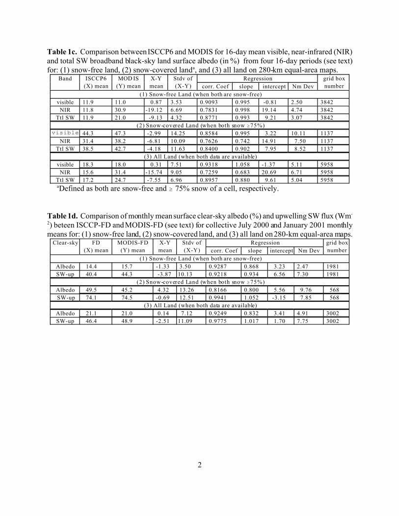
the mean (rms) differences (ISCCP6 minus SRB-ALB) are -2.0% (4.6%) and -0.3% (3.0%),respectively. But for snow-covered land and sea ice, the differences become 11.2% (6.5%) and11.0% (8.3%), respectively. We have also compared these products for seven representativevegetation types: (1) Amazon rainforest, (2) Sahara Desert, (3) snow-free grassland, (4) snow-freedeciduous forests, (5) snow-covered grassland, (6) land ice (with or without snow) and (7) sea ice.These regions are defined in the same way as above except that the snow-free vegetated regions aredefined by > 66 % coverage by the type of vegetation for a 280-km equal-area grid cell. Table 1bshows the comparison between ISCCP6-ALB and SRB-ALB for the four monthly mean clear-skyalbedos for the seven surface types. The largest biases (magnitude ! 5%) appear in Amazonrainforests and snow-covered grassland: albedo values are more difficult to be determined in theseregions because of contamination by persistent clouds and snow, respectively.Table 1c compares surface BSA for visible, NIR and total broadband SW between ISCCP6-ALB and MODIS-ALB for the four (seasonal) 16-day periods for snow-free land (defined by bothsnow maps being snow-free), snow-covered land (both maps have grid cells with ! 75% snow) andall land (all available cells for both). For snow-free land, there is a good agreement in the visibleband: mean (rms) regional differences (FD minus MODIS) are 0.9% (3.5%). Disagreement in theNIR is much greater: mean (rms) regional differences are -19% (6.7%). The MODIS retrievalalgorithm has larger errors in the NIR than in the visible (Jin et al., 2003a) because the radiancesare smaller and the atmospheric absorption is much stronger. On the other hand, the NIR albedovalues in ISCCP6-ALB rely on a surface-classification-based GCM model, which is a long-termclimatological surface representation based on Matthews [1985], but adjusted by regression withERBE to reduce systematic errors. There is not sufficient evidence to decide which of these NIR

14

results is better than the other (see next paragraph). For snow-covered land, both the agreement anddisagreement are smeared out and their mean (rms) regional differences become -3% (14%) and -6.8% (10%) for visible and NIR, respectively. The visual comparison for the seven representative vegetation types is shown in Figure 1.Figures 1a to 1c are scatter plots between ISCCP6 (=X) and MODIS (=Y) BSA for AmazonRainforests, snow-free grassland and snow-free Deciduous Forests for visible, NIR and total SW,respectively, for the same four 16-day periods (on 280-km equal-area map), and Figures 1d to 1f aretheir counterparts for snow-covered grassland, land ice, sea ice and Sahara Deserts. Because ofsparse sampling in MODIS, there are only 7 and 6 grid cells with available albedo values from allthe four periods for land ice and sea ice, and as a result, their comparisons are statisticallyinsignificant. For the other five regions, generally speaking, the figures are more or less differentfrom the mean comparison results shown in Table 1c. The Sahara desert and snow-coveredgrasslands have the highest correlations (>0.71) for all the three bands, but large mean differencesalways appear in NIR (-22% and -10% in ISCCP6 minus MODIS, respectively). The leastagreement appears in Amazon Forests (correlation coefficients are 0.46 and 0.41 for visible andNIR, respectively while their mean differences are 0.7% and -22%, respectively). Also, ISCCP6 andMODIS have better agreement in visible band than in NIR band as also shown in Table 1cTo obtain a global picture, figure 2a to 2c show the global maps of the BSA differences(ISCCP6 minus MODIS) for visible, NIR and total SW, respectively, for the 16-day period of July11 (beginning date). Again, the visible map shows that, for the majority of the world, the two datasetdiffer only within ± 5% (mean global difference = -0.5%). The largest discrepancy (up to -35%difference) appears in central Greenland (where MODIS has less data), possibly because of the

15

difficulty of identifying clear conditions over such bright regions. There is a narrow belt fromEngland to the Northeast China for essentially intensively-cultivated lands [Matthews, 1982] whereISCCP6 is 5-10% higher than MODIS. The NIR map shows large difference (mean global difference= -20%) and systematical regional-pattern dependence, indicating the two datasets have somefundamental difference in deriving the NIR albedos. The most prominent region is the North Africandeserts, where ISCCP6 is less than MODIS by > 30%. For the total broadband SW, the majority ofland areas show a difference around -10% (also the global mean difference).Table 1d shows the comparison of calculated monthly-mean surface clear-sky (apparent)albedo and upward SW between ISCCP-FD and MODIS-FD for snow-free, snow-covered and totalland. The agreement between ISCCP-FD and MODIS-FD is very good showing that the large NIRBSA differences have far less effect on the total clear-sky (apparent) albedo and upwelling SWfluxes because the atmosphere absorbs most of the SW radiation in the NIR band. For all land, themean (rms) regional differences between ISCCP and MODIS are only 0.14% (7%) and -2.5 (11)Wm-2 for the albedo and upwelling SW, respectively.Tables 2a and 2b show the comparisons of ERBE TOA clear-sky albedo with ISCCP-FD andSRB, respectively, for the four seasonal monthly means of 1986 when ERBE data is available. Forsnow- and ice-free lands, both TOA clear-sky albedos are in good agreement with ERBE: ISCCPis within 1% bias while SRB is within 2 %. This is not the case for snow-covered grassland, landand sea ice (land types 5 through 7), where ISCCP-FD exhibits a bias up to about 8% while the SRBbias is up to 13%. For snow-covered grassland (type 5), ISCCP-FD is biased high while SRB isbiased low; but for land and sea ice, both ISCCP-FD and SRB are biased low. The reasons may liepartly in their fundamentally different analysis approaches and partly in the cloud contamination for

16

ERBE. One known problem for the high latitude results in SRB, which uses the ERBE angle modelsto determine fluxes from radiances [Pinker and Laszlo, 1992], is that these angle models are biasedfor large solar zenith angles [Suttles et al., 1992].Although ISCCP-FD and MODIS have mean regional differences of -7.6% for surface BSA(based on four 16-day periods and all land areas), these differences produce TOA clear-sky albedomean (rms) differences of only -0.31% (3.4%) (not shown) because TOA albedo is insensitive tosurface NIR albedo, the visible band contributing most to the SW fluxes at TOA. Table 2c and 2dcompare monthly mean TOA clear-sky albedos from CERES (ERBE-like) with those from ISCCP-FD and MODIS-FD, respectively, for July 2000 and January 2001. The bias of ISCCP-FD withrespect to CERES (-0.29%) is slightly smaller than for MODIS-FD (0.70%) for snow-free land, butthe rms difference is slightly larger (2.4%) than for MODIS (1.7%). For snow-covered land, ISCCPhas a larger bias (4.6%) and rms difference (11%) than MODIS (3.0%, 9.8%). For all land, ISCCP-FD and MODIS have biases (rms) = 0.90% (5.7%) and 1.2% (4.5%), respectively. Both albedoproducts produce good agreement with the CERES albedos on average but ISCCP exhibits morescatter relative to CERES than MODIS does. These statistics do not provide strong evidence forchoosing between these two albedo products. Figure 3 shows the scatter plots of TOA clear-skyupward SW fluxes from CERES against the results from ISCCP-FD and MODIS-FD for snow-freeand snow-covered land areas. From figures 3a and 3b (snow-free land), we see that MODIS appearsto perform slightly better than ISCCP: the points off the diagonal (> 110 Wm"2) in Figure 3a arelocated in Northern Africa and the Arabian Peninsula, where ISCCP is biased low. The fact that thepattern of disagreement for snow-covered land shown in figure 3c and 3d is the same for bothISCCP-FD and MODIS-FD suggests that this disagreement might be partly caused by the ERBEangle models for this surface type.

17

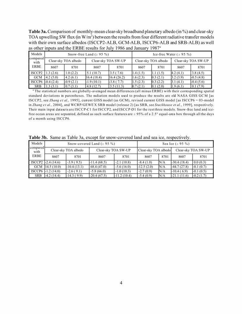
Table 3a (for snow-free land and ice-free ocean) and 3b (for snow-covered land and sea ice)compare TOA albedo and upwelling SW fluxes for clear-sky scenes with ERBE for ISCCP2-ALB,GCM-ALB, ISCCP6-ALB and SRB-ALB. The albedo and fluxes are calculated from theircorresponding surface broadband BSA or clear-sky albedo, whichever applies. From the first threeentries, we can see that adjusting the GCM albedo using the ISCCP visible reflectances for landimproved the albedo/flux comparison substantially. Going to six wavelength ranges also providessome overall improvement over the original two-wavelength-range treatment. For snow-free landand ice-free water regions, the SRB-ALB results are comparable with ISCCP6-ALB, i.e., both havea good agreement with ERBE, but for snow-covered land and sea ice regions, SRB-ALB has a largerbias than ISCCP6-ALB. There are three notable conclusions. First, except for GCM-ALB, all of theother products are adjusted to agree with ERBE in some way, yet the remaining regional scatter insurface albedo for snow-free land or ice-free water is still several percent, and even larger forsnow/ice surfaces. Second, although the reconstruction of surface albedo from a surfacevegetation/land use classification produces a fairly accurate result as shown for NASA GISS GCMmodel (which can be compared with other major GCM results), use of the ISCCP visible reflectancedata improves the result, which implies that there is significant regional (and temporal) variation inthe albedo of surfaces with the same classification [cf. Matthews and Rossow, 1987]. Third, it is stillpossible to improve surface albedo maps by producing and using better satellite-based surfacealbedo datasets. We note that MODIS is the first imaging instrument to provide measurements atwavelengths covering the whole solar spectrum.Figure 4 shows the zonal mean TOA clear-sky albedo from ISCCP6-ALB (from ISCCP-FD),SRB-ALB and ERBE for July 1986 and January 1987. In most zones, the former two arecomparable and exhibit biases with ERBE # 5% or so. In the winter hemispheres, at about 40°S-

18

55°S for July and 30°N-45°N for January, SRB performs better than ISCCP-FD, while in summerhemispheres, ISCCP usually performs better than SRB. In the polar regions, ISCCP-FD values arecloser (especially in January) to ERBE than SRB.2.2. Infrared EmissivityA. DatasetsInfrared emission from the surface depends on both temperature, which varies rapidly in timeespecially for land, and emissivity that varies with wavelength and surface properties in a complexway. Emissivity also plays an important role in determining surface temperature by remote sensing[e.g., Becker, 1987]. Because the thermal (LW) emissivity at the Earth’s surface is close to unity,most applications assume it to be unity [Peixoto and Oort, 1992], which is also the case in Zhanget al. [1995]. As a result, there were no high-quality global surface emissivity datasets determinedfrom satellite observations (3I produces emissivity at 50 Ghz, see also Prigent et al., [1997 and2000], but not for thermal radiation spectral range) or otherwise at the start of this work. The onlyglobal databases for this surface property (in terms of LW flux calculation) are constructed bycombining field and laboratory measurements of the emissivities of various rock, soil and vegetationtypes, which are generally only measured for wavelengths < 20 !m, with a surface classificationsand theoretical calculations (especially for water as in the GISS climate model, where the emissivity= 1 - albedo and the albedo is calculated using Fresnel reflection as explained before). Since July 2001, there has appeared several versions (still kept updating) of the MODIS-based high-spatial-resolution Land Surface Temperature product that also includes emissivity, whichis for 6 wavelength bands, ranging from 3.66 to 12.17 !m [see e.g., Wan et al., 2004]. Because thisproduct is only for several narrow bands and still being validated, we do not used it in this study.

19

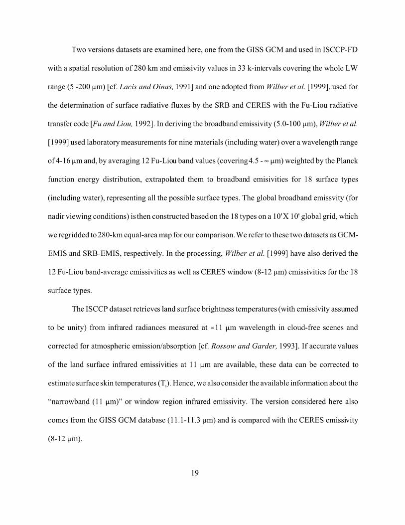
Two versions datasets are examined here, one from the GISS GCM and used in ISCCP-FDwith a spatial resolution of 280 km and emissivity values in 33 k-intervals covering the whole LWrange (5 -200 !m) [cf. Lacis and Oinas, 1991] and one adopted from Wilber et al. [1999], used forthe determination of surface radiative fluxes by the SRB and CERES with the Fu-Liou radiativetransfer code [Fu and Liou, 1992]. In deriving the broadband emissivity (5.0-100 !m), Wilber et al.[1999] used laboratory measurements for nine materials (including water) over a wavelength rangeof 4-16 !m and, by averaging 12 Fu-Liou band values (covering 4.5 - $ !m) weighted by the Planckfunction energy distribution, extrapolated them to broadband emisivities for 18 surface types(including water), representing all the possible surface types. The global broadband emissvity (fornadir viewing conditions) is then constructed based on the 18 types on a 10' X 10' global grid, whichwe regridded to 280-km equal-area map for our comparison. We refer to these two datasets as GCM-EMIS and SRB-EMIS, respectively. In the processing, Wilber et al. [1999] have also derived the12 Fu-Liou band-average emissivities as well as CERES window (8-12 !m) emissivities for the 18surface types.The ISCCP dataset retrieves land surface brightness temperatures (with emissivity assumedto be unity) from infrared radiances measured at %11 !m wavelength in cloud-free scenes andcorrected for atmospheric emission/absorption [cf. Rossow and Garder, 1993]. If accurate valuesof the land surface infrared emissivities at 11 !m are available, these data can be corrected toestimate surface skin temperatures (Ts). Hence, we also consider the available information about the“narrowband (11 !m)” or window region infrared emissivity. The version considered here alsocomes from the GISS GCM database (11.1-11.3 !m) and is compared with the CERES emissivity(8-12 !m).

20

B. Comparison of Broadband EmissivitiesFigure 5 shows a map of the differences of broadband emissivities between GCM-EMIS andSRB-EMIS. Values over land generally agree to within ±2%, but the coherent features exhibited inthe figure suggest regional differences in classification. The GCM-EMIS values tend to besomewhat larger than the SRB-EMIS values for denser vegetation types (e.g., rainforests) and forsome heavily cultivated locations (e.g., Europe and China, but not in Southern Africa), andsomewhat smaller than SRB-EMIS for intermediate density grasslands (e.g, the Russian Steppes,central US) and most of middle/southern Africa (from dense forest to grass savanna), formountainous terrains and even smaller in frozen areas (e.g., Greenland and Antarctic).Surprisingly, the largest differences are for open water (and ice/snow), ranging up to 7%. TheSRB water emissivity neglects not only the strong spectral dependence [since its broadbandemissivity is extrapolated from 12-band-averages over 4-16 !m (weighted with the Planck functionenergy distribution)], but also zenith angle variations and windspeed effects. Averaging over allzenith angles produces an emissivity, even at “window” infrared wavelengths that is lower than thenadir value (usually measured in a laboratory). Wind roughening of the surface is equivalent to re-distributing the zenith angles, but this has only a weak effect on the angle-averaged emissivity. Fora calm ocean surface, the emissivity (actually the reflectivity) can be accurately calculated using theFresnel reflection formula [e.g., Liou, 2002], and under windy conditions, such calculations can bedone with sufficiently high precision using a wave-slope distribution model as used in the GISSmodel. Figure 6a illustrates the variations of the GISS GCM emissivity values for water atwavelengths from 0.2 to 200 !m and surface wind speed = 3 m/s for cosine zenith angles 0.1, 0.5

21

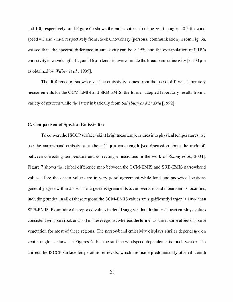
and 1.0, respectively, and Figure 6b shows the emissivities at cosine zenith angle = 0.5 for windspeed = 3 and 7 m/s, respectively from Jacek Chowdhary (personal communication). From Fig. 6a,we see that the spectral difference in emissivity can be > 15% and the extrapolation of SRB’semissivity to wavelengths beyond 16 !m tends to overestimate the broadband emissivity [5-100 !mas obtained by Wilber et al., 1999].The difference of snow/ice surface emissivity comes from the use of different laboratorymeasurements for the GCM-EMIS and SRB-EMIS, the former adopted laboratory results from avariety of sources while the latter is basically from Salisbury and D’Aria [1992]. C. Comparison of Spectral EmissivitiesTo convert the ISCCP surface (skin) brightness temperatures into physical temperatures, weuse the narrowband emissivity at about 11 !m wavelength [see discussion about the trade offbetween correcting temperature and correcting emissivities in the work of Zhang et al., 2004].Figure 7 shows the global difference map between the GCM-EMIS and SRB-EMIS narrowbandvalues. Here the ocean values are in very good agreement while land and snow/ice locationsgenerally agree within ± 3%. The largest disagreements occur over arid and mountainous locations,including tundra: in all of these regions the GCM-EMIS values are significantly larger (> 10%) thanSRB-EMIS. Examining the reported values in detail suggests that the latter dataset employs valuesconsistent with bare rock and soil in these regions, whereas the former assumes some effect of sparsevegetation for most of these regions. The narrowband emissivity displays similar dependence onzenith angle as shown in Figures 6a but the surface windspeed dependence is much weaker. Tocorrect the ISCCP surface temperature retrievals, which are made predominantly at small zenith

22

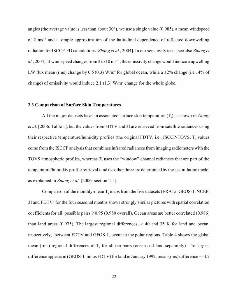
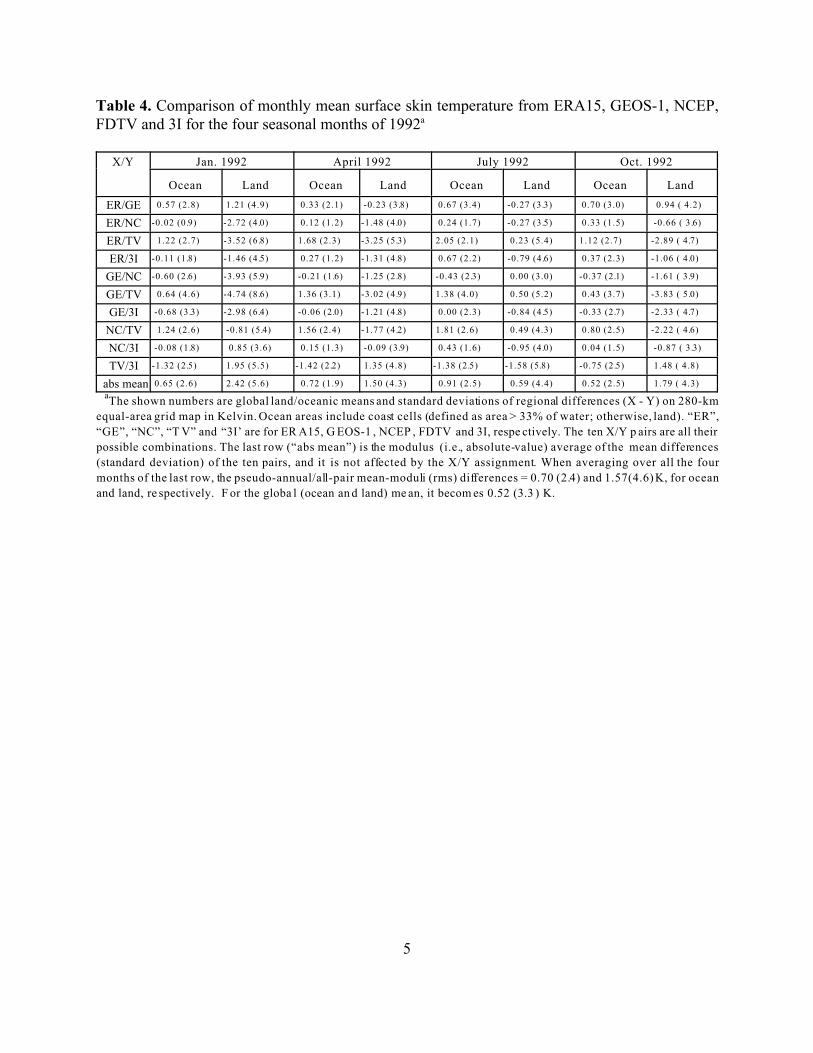
angles (the average value is less than about 30°), we use a single value (0.985), a mean windspeedof 2 ms"1 and a simple approximation of the latitudinal dependence of reflected downwellingradiation for ISCCP-FD calculations [Zhang et al., 2004]. In our sensitivity tests [see also Zhang etal., 2004], if wind speed changes from 2 to 10 ms"1, the emissivity change would induce a upwellingLW flux mean (rms) change by 0.5 (0.3) W/m2 for global ocean, while a ±2% change (i.e., 4% ofchange) of emissivity would induce 2.1 (1.3) W/m2 change for the whole globe.2.3 Comparison of Surface Skin TemperaturesAll the major datasets have an associated surface skin temperature (Ts) as shown in Zhanget al. [2006: Table 1], but the values from FDTV and 3I are retrieved from satellite radiances usingtheir respective temperature/humidity profiles (the original FDTV, i.e., ISCCP-TOVS, Ts valuescome from the ISCCP analysis that combines infrared radiances from imaging radiometers with theTOVS atmospheric profiles, whereas 3I uses the “window” channel radiances that are part of thetemperature/humidity profile retrieval) and the other three are determined by the assimilation modelas explained in Zhang et al. [2006: section 2.1].Comparison of the monthly-mean Ts maps from the five datasets (ERA15, GEOS-1, NCEP,3I and FDTV) for the four seasonal months shows strongly similar pictures with spatial correlationcoefficients for all possible pairs !0.95 (0.980 overall). Ocean areas are better correlated (0.986)than land areas (0.975). The largest regional differences, > 40 and 35 K for land and ocean,respectively, between FDTV and GEOS-1, occur in the polar regions. Table 4 shows the globalmean (rms) regional differences of Ts for all ten pairs (ocean and land separately). The largestdifference appears in (GEOS-1 minus FDTV) for land in January 1992: mean (rms) difference = -4.7

23

(8.6) K. The overall modulus mean difference (i.e., absolute values of the mean differences, notaffected by subtraction order, see e.g., Reynolds [1988]) (rms difference) is 0.52 (3.3) K (Table 4footnotes), very similar to the modulus mean (rms) difference for surface air temperature Ta, 0.53(2.6) in Zhang et al. [2006]. Like Ta, the global bias arises from a partial cancellation between landand ocean biases: if land and ocean are separated, the modulus mean (rms) difference of Ts is 1.57(4.6) and 0.70 (2.4), respectively, compared with 0.73 (3.7) and 0.77 (1.9) for Ta. The land Tsmodulus mean bias is twice that of Ta while the ocean values are comparable.Figure 8 illustrates the zonal monthly mean differences (all minus FDTV). The largestdifferences, up to 20 K, appear in the polar regions, where cloud contamination makes retrievalsvery difficult. In fact, wintertime polar regimes also exhibit larger clear-sky biases in Ts [cf. Curryet al., 1996]. However, the reanalyses also exhibit the well-known cold biases at these latitudes. Formost lower and middle latitudes, the differences are generally " 5 K and < 3 K for land and ocean,respectively. There is a systematic tendency for the reanalyses to be slightly colder in winter andwarmer in summer over land relative to FDTV, despite the fact that the original ISCCP Ts retrievalshave clear sky biases (too cold in winter, too warm in summer) [Rossow and Garder, 1993] thathave been reduced in the FD analysis [Zhang et al., 2004]. We have collected three additional SST products: (1) NOAA/NASA Pathfinder AdvancedVery High Resolution Radiometer (AVHRR) (descending and ascending) version 4.0 with 9km/daily resolution and global coverage for 1981 to the current, produced by JPL/Caltech (estimatederror is given as 0.5-0.7 K [Vazquez et al., 1998]); (2) NOAA Optimum Interpolation Sea SurfaceTemperature Analysis version OI.V1 (1983-2000) and V2 (2000-2001) with 1°/weekly resolutionand also global coverage [Reynolds, et al., 2002]; and (3) The Tropical Rainfall Measuring Mission

24

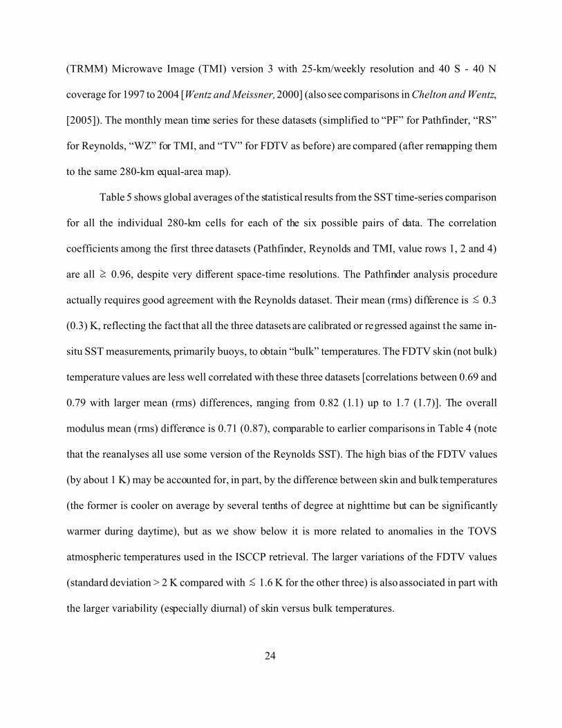
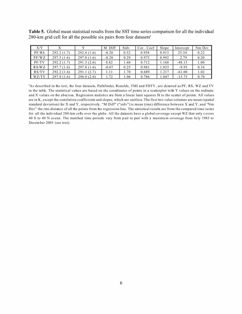
(TRMM) Microwave Image (TMI) version 3 with 25-km/weekly resolution and 40 S - 40 Ncoverage for 1997 to 2004 [Wentz and Meissner, 2000] (also see comparisons in Chelton and Wentz,[2005]). The monthly mean time series for these datasets (simplified to “PF” for Pathfinder, “RS”for Reynolds, “WZ” for TMI, and “TV” for FDTV as before) are compared (after remapping themto the same 280-km equal-area map).Table 5 shows global averages of the statistical results from the SST time-series comparisonfor all the individual 280-km cells for each of the six possible pairs of data. The correlationcoefficients among the first three datasets (Pathfinder, Reynolds and TMI, value rows 1, 2 and 4)are all ! 0.96, despite very different space-time resolutions. The Pathfinder analysis procedureactually requires good agreement with the Reynolds dataset. Their mean (rms) difference is " 0.3(0.3) K, reflecting the fact that all the three datasets are calibrated or regressed against the same in-situ SST measurements, primarily buoys, to obtain “bulk” temperatures. The FDTV skin (not bulk)temperature values are less well correlated with these three datasets [correlations between 0.69 and0.79 with larger mean (rms) differences, ranging from 0.82 (1.1) up to 1.7 (1.7)]. The overallmodulus mean (rms) difference is 0.71 (0.87), comparable to earlier comparisons in Table 4 (notethat the reanalyses all use some version of the Reynolds SST). The high bias of the FDTV values(by about 1 K) may be accounted for, in part, by the difference between skin and bulk temperatures(the former is cooler on average by several tenths of degree at nighttime but can be significantlywarmer during daytime), but as we show below it is more related to anomalies in the TOVSatmospheric temperatures used in the ISCCP retrieval. The larger variations of the FDTV values(standard deviation > 2 K compared with " 1.6 K for the other three) is also associated in part withthe larger variability (especially diurnal) of skin versus bulk temperatures.

25

The zonal-mean differences between these three SST datasets and FDTV for January andJuly, 2000 (not shown) exhibit the same patterns as shown in Figure 8, i.e., the biases betweenFDTV and the reanalyses (and 3I) are similar to those with the Reynolds SST, which is used invarious ways as a standard for all the others. The larger polar differences are all associated withincreasing sea ice fraction: the other SST products report water temperature, not the ice surfacetemperature as does FDTV. Excluding the polar regions, the difference between FDTV and the otherdatasets is generally " 2 K. Figures 9a and 9b also show the differences in the SST anomaly timeseries (all minus FDTV) for global and tropical averages, respectively. Much of the large-amplitudevariations of the other datasets relative to FDTV are induced in the ISCCP-retrieved Ts values byspurious temperature/humidity changes in the original TOVS as noted in Zhang et al.[2006: section2.1]). Because the difference of Ts and Ta controls the net LW at the surface, Zhang et al. [2006:Section 2.9 and Figure 11] also compared the differences (Ts minus Ta) from FDTV with those from3I and the three reanalyses but we do not repeat it here. 3. Summary and DiscussionEstimating the surface radiation budget has long been pursued [Simpson, 1929] because,together with latent and sensible heat fluxes, it comprises one fundamental coupling of theatmosphere with the ocean and land surfaces. Direct estimates that resolve regional and weather-scale variability with reasonable accuracy have only become possible with the advent of completeglobal, mostly satellite, datasets within the past couple of decades. Zhang et al. [2004] now estimatethat surface radiative fluxes can be determined to within about 10-15 W/m2 (regional monthly mean

26

flux values), improved by about 5 W/m2 over Rossow and Zhang [1995]. The main limitation is stillthe accuracy of the input datasets. Sensitivity studies using ISCCP-based-estimates (“realistically-assumed”) of the input uncertainties [based, in part, on the analysis presented here and in the workof Zhang et al., 1995; 2004; 2006] show that the leading uncertainties in the surface fluxes are nolonger predominantly induced by clouds but are now as much associated with uncertainties in thesurface and near-surface atmospheric properties.This study presents a fuller, more quantitative evaluation of these uncertainties for thesurface albedo and emissivity, and surface skin temperatures by comparing the main available globaldatasets that are treated as an ensemble of realizations of the actual climate such that theirdifferences represent an estimate of the uncertainty in their values because we do not know the“truth”. The results are globally representative and may be taken as a generalization of our previousISCCP-based estimates in Zhang et al. [1995; 2004]. Generally speaking, the radiative fluxuncertainties induced by the input uncertainties from Zhang et al. [2006] and this study areconsistent with the flux uncertainty estimates in Zhang et al. [2004] based on all of our past andcurrent sensitivity studies, and therefore, in order to meet the accuracy requirements forclimatological studies, say within 10 W/m2, we still need substantial improvements of those inputparameters that contribute major errors as summarized in the work of Zhang et al. [2006] and below.The main conclusions of this study, together with all the radiative flux sensitivity studies wehave done previously, are as follows. (1) The uncertainty in global mean (rms) for regionaldifferences for visible, NIR and total SW black-sky albedo (land only) is 0.3% (7.5%), 16% (9%)and 7.6% (7%), respectively. Although land surface albedos in the NIR remain poorly constrained,

27

they do not cause too much error in SW fluxes because the atmosphere absorbs much of theradiation in this wavelength range. Nevertheless, the subtle geographic and seasonal variations ofsurface absorbed SW depend on variations of the NIR albedo influenced by the precise mixture ofsoil/rock, vegetation and snow and the seasonal variations of vegetation activity and snow. Themean (rms) difference of 7.6% (7%) in broadband black-sky SW albedo disagreement for landsurface from this study leads to the uncertainty estimate of about 7%, which can easily induce 5-10W/m2 uncertainty in (upwelling) surface SW flux estimates. But the full potential of satellite sensorslike MODIS or the MEdium Resolution Imaging Spectrometer Instrument (MERIS) that sample(nearly) the complete solar wavelength range to produce definitive surface albedo maps withrelatively high space-time resolution has not yet been achieved. The current 16-day period MODISalbedo, though having very high spatial resolution, is usually not globally complete. The currentproduct is also produced with a 16-day time resolution. Most importantly, the current productcorrects for atmospheric effects with a relatively crude climatology of atmospheric composition andaerosols: neglecting the detailed space-time variations of water vapor, in particular, makes theuncertainties for the NIR albedo large. These limitations are not inherent; given the available dataproducts specifying the ozone, water vapor and aerosol abundances as functions of location andtime, a much more intensive analysis of the MODIS radiances is possible. However, to obtain thesurface radiative fluxes over the whole time period of the ISCCP-FD product, the MODIS productmust be used to “calibrate” the longer AVHRR record for surface albedo. (2) In the same way, theuncertainty for broadband and window emissivity may be taken as about 3-5%. Even though thedisagreement between the two surface LW emissivity reconstructions appear to be relatively large,the fact that this disagreement is confined to wavelengths > 20 !m means that it has little practicaleffect (1-3 W/m2) on the surface upwelling LW fluxes because the atmosphere is nearly opaque at

28

these wavelengths, so reflected downwelling radiation almost balances the reduction of upwellingradiation (this near-balance is not true in the polar regions but there the fluxes are much smaller inmagnitude). (3) The uncertainty in the skin temperatures is about 3 K. It is one of the two leadingfactors that cause problems with surface LW fluxes. Even though the disagreements among thevarious datasets are generally only 2-4 K, this can easily cause 10-15 W/m2 uncertainty in surface(upwelling) LW calculation.The overall summary, based on both Zhang et al. [2006] and this work, is as follows.For surface LW fluxes, significant improvements could be obtained by improving the retrievals of(in order of decreasing importance): (1) surface skin temperature, (2) surface air and near-surface-layer temperature, (3) column precipitable water amount and (4) broadband emissivity. As we haveshown the retrieval of surface skin and air temperatures are linked because the relevant satellitemeasurements are sensitive to both so they should be retrieved together [cf. Aires et al., 2002].Moreover, the systematic differences between clear- and cloudy-sky skin temperatures requiresextension of the analysis of infrared measurements to include microwave measurements [cf. Prigentet al., 2003]. Some improvement in surface emissivities over a limited wavelength range may comefrom a careful analysis of the new infrared spectrometers, such as the Atmospheric Infrared Sounder[AIRS, see Olsen, 2005]. For surface SW fluxes, improvements could be obtained (excludingimproved cloud treatment) by improving the retrievals of (1) aerosols (from our sensitivity studiesbut not discussed in this work), and (2) surface (black-sky) albedo, of which, NIR has largeruncertainty. Surface albedo and aerosols are also linked since satellite measurements at solarwavelengths are generally sensitive to both, especially over land, suggesting again, that the bestresults would be obtained by retrieving both together.

29

Acknowledgments. We thank Crystal B. Schaaf, Feng Gao and Yufang Jin for supplying their MODIS-retrievedalbedo datasets and giving instructions on how to use them. We thank Calleen Mikovitz and SteveCox for supplying the ERA15, GEOS-1 and SRB datasets. We also thank Jacek Chowdhary forsupplying the values for Figure 6 from his theoretical calculation. The work has been funded by theNASA Radiation Sciences Program (D. Anderson and H. Maring). We appreciate all the beneficialcomments and suggestions from two anonymous reviewers that help improve this publication.

30

REFERENCESAires, F., A. Chedin, N.A. Scott and W.B. Rossow (2002), A regularized neural net approach forretrieval of atmospheric and surface temperatures with the IASI instrument. J. Appl. Meteor., 41,144-159..Becker, F. (1987), The impact of spectral emissivity on the measurement of land surface temperaturefrom a satellite. Int. J. Remote Sens., 8, 1509–1522.Briegleb, B.P., P. Minnis, V. Ramanathan and E. Harrison (1986), Comparison of regional clear-skyalbedos inferred from satellite observations and model calculations, J. Clim. Appl. Meteor., 25, 214-226. Chelton, D.B., and F.J. Wentz (2005), Global microwave satellite observations of sea surfacetemperature for numerical weather prediction and climate research, Bull. Amer. Meteor. Soc., 86,1097-1115.Chen, C.-T. and E. Roeckner (1996), Validation of the Earth radiation budget as simulated by theMax Planck Institute for Meteorology general circulation model ECHAM4 using satelliteobservations of the Earth Radiation Budget Experiment, J. Geophys. Res., 101, 4,269-4,287.Cox, C and W. Munk (1956), Slopes of the sea surface deduced from photographs of the sun glitter,Bull. Scripps Inst. Oceanogr., 6, 401-488.Curry, J.A., W.B. Rossow, D. Randall and J.L. Schramm (1996), Overview of arctic cloud andradiation characteristics, J. Climate, 9, 1731-1760.Csiszar, I. And G. Gutman (1999), Mapping global land syrface albedo from NOAA AVHRR, J.Geophys. Res., 104, 6,215-6,228.Darnell, W.L. and W.F. Staylor (1992), Seasonal variation of surface radiation budget derived fromInternational Satellite Cloud Climatology Project C1 data, J. Geophys. Res., 97, 15,741-15760.Fu, Q. and K.N. Liou (1992), On the correlated k-distribution method for radiative transfer innonhomogeneous atmosphere, J. Atmos. Sci, 49, 2139-2156.Gibson, J.K., P. Kållberg, S. Uppala, A. Hernandez, A. Nomura and E. Serrano (1999), ECMWF re-analysis project report series, 1. ERA-15 description,(version 2 - January 1999), European Centrefor Medium-Range Weather Forecasts.Govaerts, Y.M., A. Lattanzio, B. Pinty and J. Schmetz (2004), Consistent surface albedo retrievalfrom two adjacent geostationary satellites, Geophys. Res. Letters, 31, L15201, doi:10.1029/2004GL020418.Gupta, S.K., D.P. Kratz, P.W. Stackhouse, Jr., and Anne C. Wilber (2001), The Langley

31

parameterized shortwave algorithm (LPSA) for surface radiation budget studies, version 1.0,NASA/TP-2001-211272, NASA, 26 pp.Hansen, J., G. Russell, D. Rind, P. Stone, A. Lacis, S. Lebedeff, R. Ruedy, and L. Travis (1983),Efficient three-dimensional global models for climate studies: Model I and II, Mon. Weather Rev.,111, 609-662.Henderson-Sellers, A. and M.F. Wilson (1983), Surface albedo data for climate modeling, Rev.Geophys. Space Phys., 21, No. 8, 1743-1778.Jin, Yufang, C.B. Schaaf, C.E. Woodcock, F. Gao, X. Li and A.H. Strahler (2003a), Consistency ofMODIS surface bidirectional reflectanve distribution function and albedo retrieval: 1. Algorithmperformance, J. Geophys. Res., 108(D5), 4158, doi:10.1029/2002JD002803.Jin, Yufang, C.B. Schaaf, C.E. Woodcock, F. Gao, X. Li and A.H. Strahler (2003b), Consistencyof MODIS surface bidirectional reflectanve distribution function and albedo retrieval: 2. Validation,J. Geophys. Res., 108(D5), 4159, doi:10.1029/2002JD002804.Kalnay, E., M. Kanamitsu, R. Kistler, W. Collins, D. Deaven, L. Gandin, M. Iredell, S. Saha, G.White, J. Woollen, Y. Zhu, A. Leetmaa,,B. Reynolds, M. Chelliah, W. Ebisuzaki, W. Higgins, J.Janowiak, K.C. Mo, C. Ropelewski, J. Wang, Roy Jenne and Dennis and Joseph (1996), TheNCEP/NCAR 40-Year Reanalysis Project, Bull. Amer. Meteor. Soc., 77, No. 3, pp. 437-471.Kistler, R, E. Kalnay, W. Collins, S. Saha, G. White, J. Woollen, M. Chelliah, W. Ebisuzaki, M.Kanamitsu, V. Kousky, H. van den Dool, R. Jenne, and M. Fiorino (2001), The NCEP-NCAR 50year reanalysis: monthly means CD-ROM and documentation, Bill. Amer. Meteor. Soc., 82, No. 2.Lacis, A.A. and V. Oinas (1991), A description of the correlated k distribution method for modelingnongray gaseous absorption, thermal emission, and multiple scattering in vertically inhomogeneousatmospheres, J. Geophys. Res., 96, 9027-9063.Li, Zhanqing and L. Garand (1994), Estimate of surface albedo from space: a parameterization forglobal application, J. Geophys. Res., 99, 8,335-8,350.Liang, S., A.H. Strahler and C.W. Walthall (1999), Retrieval of land surface albedo from satelliteobservations: A simulation study, J. Appl. Meteorol., 38, 712-725.Liou, K.N. (2002), An Introduction to Atmospheric Radaition, Academic Press, New York, 583 pp.Lucht, W., C.B. Schaaf and A.H. Strahler (2000), An algorithm for the retrieval of albedo fromspace using semiempirical BRDF models, IEEE Transactions on Geoscience and Remote Sensing,38, No. 2, 977-998. Matthews, E. (1982), Global vegetation and land use: new high-resolution data bases for climate

32

studies, J. Climate Appl. Meteor., 22, 474-487.Matthews, E. (1985), Atlas of archived vegetation, land-use and seasonal albedo data sets, NASATech. Memo. 86199, 53 pp.Matthews, E., and W.B. Rossow (1987), Regional and seasonal variations of surface reflectance at0.6 !m. J. Climate Appl. Meteor., 25, 170-202.Olsen, E.T., ed. (2005), AIRS/AMSU/HSB version 4.0 data release user guide, Jet PropulsionLaboratory, California Institute of Technology, Pasadena, Ca.Peixoto, J.P. and A. H. Oort (1992), Physics of climate, American Institute of Physics, New York,520 pp.Pinker, R.T. and I. Laszlo (1992), Modeling surface solar irradiance for satellite applications onglobal scale, J. Appl. Meteor., 31, 194-211.Posey, J.W. and P.F. Clapp (1964), Global distribution of nomal surface albedo, Deofis. Int., 4, 33-48.Prigent, C., W.B. Rossow, and E. Matthews (1997), Microwave land surface emissivities estimatedfrom SSM/I observations. J. Geophys. Res. 102, 21867-21890, doi:10.1029/97JD01360. Prigent, C., J.-P. Wigneron, W.B. Rossow, and J.R. Pardo-Carrion (2000), Frequency and angularvariations of land surface microwave emissivities: Can we estimate SSM/T and AMSU emissivitiesfrom SSM/I emissivities?. IEEE Trans. Geosci. Remote Sensing 38, 2373-2386. Prigent, C., F. Aires, and W.B. Rossow (2003), Land surface skin temperatures from a combinedanalysis of microwave and infrared satellite observations for an all-weather evaluation of thedifferences between air and skin temperatures. J. Geophys. Res. 108, no. D10, 4310,doi:10.1029/2002JD002301. Reynolds, R.W. (1988), A real-time global sea surface temperature analysis, J. Climate, 1, 75-86.Reynolds, R.W., N.A. Rayner, T.M. Smith, D.C. Stokes and W. Wang (2002), An improved in situand satellite SST analysis for climate, J. Climate, 15, 1609-1625.Rossow, W.B., and L.C. Garder (1993). Validation of ISCCP cloud detections. J. Climate 6,2370-2393, doi:10.1175/1520-0442. Rossow, W.B., and A.A. Lacis (1990), Global, seasonal cloud variations from satellite radiancemeasurements. Part II: Cloud properties and radiative effects. J. Climate 3, 1204-1213,doi:10.1175/1520-0442(1990)003<1204:GSCVFS>2.0.CO;2.

33

Rossow, W.B., and R.A. Schiffer (1991), ISCCP cloud data products. Bull. Amer. Meteor. Soc.,72, 1-20.Rossow, W.B., and Y-C. Zhang (1995), Calculation of surface and top-of-atmosphere radiativefluxes from physical quantities based on ISCCP datasets, Part II: Validation and first results. J.Geophys. Res., 100, 1167-1197.Rossow, W.B., A.W. Walker, D.E. Beuschel and M.D. Roiter (1996), International SatelliteCloud Climatology Project (ISCCP) documentation of new cloud datasets, WMO/TD-No. 737,World Climate Research Programme (ICSU and WMO), 115 pp.Salisbury, J.W. and D.M. D’Aria (1992), Emissivity of terrestrial materials in the 8-14 !matmospheric window, Remote Sensing Envir., 42, 83-106.Schaaf, C.B., et al. (2002), First operational BRDF, albedo and nadir reflectance products fromMODIS, remote sens. Environ., 83, 135-148.Scott, N.A., A. Chédin, R. Armante, J. Francis, C. Stubenrauch, J-P Chaboureau, F. Chevallier,C. Claud and F. Cheruy (1999), Characteristics of the TOVS pathfinder Path-B dataset, Bull.Aner. Meteror. Soc., 80, 2679-2701Simpson, G.C., (1929): The distribution of terrestrial radiation. Mem. Roy. Meteor. Soc., 3, 53-78.Stackhouse, P.W. S.K. Gupta, S.J. Cox, M. Chiacchio and J.C. Mikovitz (1999), TheWCRP/GEWEX Surface Radiation Budget Project release 2: first results at 1 degree resolution,10th Conference on Atmospheric Radiation: A Symposium with tributes to the works of VernerE. Suomi. American Meteorological Society, Madison, Wisconsin, 28 June-2 July.Stackhouse Jr., P.W., S. J. Cox, S.K. Gupta, M.Chiacchio, and J.C., Mikovitz (2001), TheWCRP/GEWEX surface radiation budget project release 2: An assessment of surface fluxes at 1degree resolution. International Radiation Sysposium, St.-Petersburg, Russia, July 24-29, 2000.IRS 2000: Current Problems in Atmospheric Radiation, W.L. Smith and Y. Timofeyev (eds.), A.Deepak Publishing, 147. Stackhouse Jr., P.W., S.K. Gupta, S.J. Cox, J.C. Mikovitz, T. Zhang, and M. Chiacchio (2004),12-Year Surface Radiation Budget Data Set, GEWEX News, November,10-12.Staylor, W.F. and A.C. Wilber (1990), Global surface albedos estimated from ERBE data,Proceedings, 7th Conf. On Atmos. Rad., Sane Francisco.Suttles, J.T., B.A. wielicki and S. Vemury (1992), Top of atmosphere radiative fluxes:Validation of ERBE scanner inversion algorithm using Nimbus 7 ERB data, J. Appl. Meterol.,31, 784-796.Takacs, L.L., A. Molod, and T. Wang (1994), Documentation of the Goddard Earth ObservingSystem (GEOS) general circulation model - version 1, NASA Technical Memorandum 104606,Vol 1.Vazquez, J., K. Perry and K. Kilpatrick (1998), NOAA/NAA AVHRR oceans pathfinder seasurface temperature data set user’s reference manual, JPL Publication D-14070, 67 pp.

34

Wan, Z., Y. Zhang, Q. Zhang and Z.-L. Li (2004), quality assessment and validation of theMODIS global land surface temperature, Int. J. Remote Sensing, 25, No. 1, 261-274.Wentz, F.J. and T. Meissner (2000), AMSR ocean algorithm, RSS Tech. Proposal 121599 A-1,prepared for EOS Project Goddard Space Flight Center, NASA. Whitlock, C.H., T.P. Charlock, W.F. Staylor, R.T. Pinker, I. Laszlo, A. Ohmura, H. Gilgen, T.Konzelman, R.C. DiPasquale, C.D. Moats, S.R. LeCroy and N.A. Ritchey (1995), First globalWCRP shortwave surface radiation budget dataset, Bull. Amer. Meteror. Soc., 76, 905-922.Wielicki, B.A., B.R. Barkstrom, E.F. Harrison, R.B. Lee, G.L. Smith and J.E. Cooper (1996),Clouds and the Earth’s Radiant Energy System (CERES): An Earth observing systemexperiment, Bull. Amer. Meteor. Soc., 77, 853-868.Wilber, A.C., D.P. Kratz and S.K. Gupta (1999), Surface emissivity maps for use in satelliteretrievals of longwave radiation, NASA Technical Memorandum TP-1999-209362.Zhang, Y-C., W.B. Rossow and A.A. Lacis (1995), Calculation of surface and top-of-atmosphereradiative fluxes from physical quantities based on ISCCP datasets, Part I: Method and sensitivityto input data uncertainties. J. Geophys. Res., 100, 1149-1165.Zhang, Y-C., W.B. Rossow, A.A. Lacis, V. Oinas and M.I. Mishchenko (2004), Calculation ofradiative fluxes from the surface to top-of-atmosphere based on ISCCP and other global datasets:Refinements of the radiative transfer model and the input data, J. Geophys. Res., 109, D19105,doi:10.1029/2003JD004457.Zhang, Y-C., W.B. Rossow and P.W. Stackhouse Jr. (2006), Comparison of different globalinformation sources used in surface radiative flux calculation: Radiative Properties of the Near-surface Atmosphere (submitted to J. Geophys. Res., in print).

35

FIGURE CAPTIONSFigure 1a. Scatter plot of visible black-sky albedo (in %) for Amazon Rainforests (dark greydiamond), snow-free Grassland (empty circle) and snow-free deciduous forests (solid triangle)from ISCCP6 and MODIS for four 16-day periods (beginning on April 6, July 11 and September29, 2000, and January 17, 2001).Figure 1b. Same as 1a but for near-infrared and the diagonal line is not plotted from origin (0,0),but from the point that visually approximately reflect their mean bias for all the correspondingregions. .Figure 1c. Same as 1b but for total SW (visible and near-infrared).Figure 1d. Scatter plot of visible black-sky albedo (in %) for snow-covered grassland (emptytriangle), land ice (dark grey square), sea ice (solid triangle) and Sahara deserts (dark greydiamond) from ISCCP6 and MODIS for four 16-day periods (beginning on April 6, July 11 andSeptember 29, 2000, and January 17, 2001).Figure 1e. Same as 1d but for near-infrared and the diagonal line is not plotted from origin (0,0),but from the point that visually approximately reflect their mean bias for all the correspondingregions.Figure 1f. Same as 1e but for total SW (visible and near-infrared).Figure 2a. Global map of differences (ISCCP6 minus MODIS) of visible black-sky albedo (in%) from four 16-day periods (beginning on April 6, July 11 and September 29, 2000, andJanuary 17, 2001).Figure 2b. Same as 2a but for near-infrared. Figure 2c. Same as 2a but for total SW (visible and near-infrared).Figure 3a. Scatter plot of monthly-mean TOA clear-sky SW-up fluxes (in W/m2) for snow-freeland from ISCCP-FD and CERES, accumulated from January and July 1992.Figure 3b. Same as figure 3a but for MODIS-FD and CERES.Figure 3c. Same as figure 3a but for snow-covered land.Figure 3d. Same as figure 3b but for snow-covered land.Figure 4a. Comparison of zonal monthly-mean TOA clear-sky albedo (in %) from ISCCP-FD,SRB and ERBE for July 1986.

36

Figure 4b. Same as figure 4a but for January 1987.Figure 5. Global map of differences (ISCCP-FD minus SRB) of broadband emissivities (in %)from ISCCP-FD 1992 annual mean and SRB climatology.Figure 6a. Water emissivity from theoretical calculation using NASA GISS model (see text) atwind speed = 3 m/s for cosine zenith view angle = 0.1, 0.5 and 1.0, respectively. Figure 6b. Same as figure 6a but for a fixed cosine zenith view angle = 0.5 and for wind speed =3 and 7 m/s, respectively.Figure 7. Global map of differences (ISCCP-FD minus SRB) of window-region emissivities (in%) from ISCCP-FD 1992 annual mean and SRB climatology.Figure 8a. Difference of zonal monthly-mean surface skin temperature (in K) for ERA15,GEOS-1, NCEP and 3I minus FDTV, respectively (as TS01ertv for ER - TV, etc.), for land andJanuary 1992.Figure 8b. Same as figure 8a but for July 1992.Figure 8c. Same as figure 8a but for ocean.Figure 8d. Same as figure 8b but for oceanFigure 9a. Difference of the time series of global mean SST (in K) from Pathfinder (PF),Reynolds (RS) and TMI (WZ) minus FDTV (TV), respectively.Figure 9b. Same as figure 9a but for 30 S - 30 N mean.

1

TABLESTable 1a. Comparison between ISCCP6 and SRB for monthly-mean broadband clear-sky surfacealbedoa for snow-free land, ice-free water, snow-covered land and sea iceb for January, April, July,October, 1992: globally-averaged mean difference (ISCCP6 minus SRB) with its spatial standarddeviation in parentheses from 280-km equal-area maps. Last row shows the mean values of theabove four months.Snow-free Land Ice-free Water Snow-covered Land Sea Ice9201 -1.7 ( 5.8) -0.7 ( 1.9) 15.0 ( 11.4) 20.6 ( 16.8)9204 -1.0 ( 4.5) -0.3 ( 3.8) 10.9 ( 3.5) 7.5 ( 6.4)9207 -3.4 ( 3.8) -0.4 ( 4.4) 7.1 ( 4.8) 8.1 ( 3.8)9210 -2.0 ( 4.4) 0.0 ( 2.1) 11.7 ( 6.3) 7.8 ( 6.1)mean -2.0 ( 4.6) -0.3 ( 3.0) 11.2 ( 6.5) 11.0 ( 8.3) aIn % bDefined as ! 95% of a grid box thro ugh all the da ys of a mo nth using IS CCP sn ow and ice data. Table 1b. Comparison between ISCCP6 and SRB for monthly-mean broadband clear-sky surfacealbedo a, collected from the four months (Table 1a) for seven regionsbregionnumber ISCCP6(X) mean SRB(Y) mean X-Ymean Stdv of(X-Y) Regression grid boxnumbercorr. Coef slope intercept Nm Dev 1 14.5 19.9 -5.4 1.9 0.714 1.4 0.1 0.8 160 2 32.8 29.9 2.9 4.3 0.766 0.8 3.6 3.0 484 3 15.2 16.2 -1.1 3.5 0.515 0.8 3.5 2.4 150 4 11.6 14.0 -2.4 3.1 0.607 0.9 3.6 2.2 277 5 54.5 44.0 10.5 4.9 0.973 0.8 4.8 2.5 33 6 76.6 73.2 3.4 2.6 -0.280 0.9 2.2 2.1 152 7 69.0 61.0 8.0 6.1 0.773 0.8 4.8 3.5 274 aIn % bAs numbered in column one, the seven types of land features (based on ISCCP surface information) are: (1) Amazonrainforests (2) Sahara Deserts, (3) Snow-free grassland, (4) Snow-free deciduous forests, (5) Snow-covered grassland,(6) Land ice (w ith or withou t snow co ver), and (7) S ea ice. All surface features (other than vegetation types) are definedwhen such features > 95% of a 280-km equal-area box and all vegetation types are defined as they are > 66% of a gridbox. “Nm Dev” is the RM S distance o f all points from the regressio n line, “corr.co ef” correlation coefficient, and “stdv”standard deviation.

2

Table 1c. Comparison between ISCCP6 and MODIS for 16-day mean visible, near-infrared (NIR)and total SW broadband black-sky land surface albedo (in %) from four 16-day periods (see text)for: (1) snow-free land, (2) snow-covered landa, and (3) all land on 280-km equal-area maps.Band ISCCP6(X) mean MOD IS(Y) mean X-Ymean Stdv of(X-Y) Regression grid boxnumbercorr. Coef slope intercept Nm Dev(1) Snow-free Land (when both are snow-free)visible 11.9 11.0 0.87 3.53 0.9093 0.995 -0.81 2.50 3842NIR 11.8 30.9 -19.12 6.69 0.7831 0.998 19.14 4.74 3842Ttl SW 11.9 21.0 -9.13 4.32 0.8771 0.993 9.21 3.07 3842(2) Snow-covered Land (when both snow !75%)visible 44.3 47.3 -2.99 14.25 0.8584 0.995 3.22 10.11 1137NIR 31.4 38.2 -6.81 10.09 0.7626 0.742 14.91 7.50 1137Ttl SW 38.5 42.7 -4.18 11.63 0.8400 0.902 7.95 8.52 1137(3) All Land (when both data are available)visible 18.3 18.0 0.31 7.51 0.9318 1.058 -1.37 5.11 5958NIR 15.6 31.4 -15.74 9.05 0.7259 0.683 20.69 6.71 5958Ttl SW 17.2 24.7 -7.55 6.96 0.8957 0.880 9.61 5.04 5958 aDefined as both are snow-free and ! 75% snow of a cell, respectively. Table 1d. Comparison of monthly mean surface clear-sky albedo (%) and upwelling SW flux (Wm-2) beteen ISCCP-FD and MODIS-FD (see text) for collective July 2000 and January 2001 monthlymeans for: (1) snow-free land, (2) snow-covered land, and (3) all land on 280-km equal-area maps.Clear-sky FD(X) mean MODIS-FD(Y) mean X-Ymean Stdv of(X-Y) Regression grid boxnumbercorr. Coef slope intercept Nm Dev(1) Snow-free Land (when both are snow-free)Albedo 14.4 15.7 -1.33 3.50 0.9287 0.868 3.23 2.47 1981SW-up 40.4 44.3 -3.87 10.13 0.9218 0.934 6.56 7.30 1981(2) Snow-covered Land (when both snow !75%)Albedo 49.5 45.2 4.32 13.26 0.8166 0.800 5.56 9.76 568 SW-up 74.1 74.5 -0.69 12.51 0.9941 1.052 -3.15 7.85 568(3) All Land (when both data are available)Albedo 21.1 21.0 0.14 7.12 0.9249 0.832 3.41 4.91 3002SW-up 46.4 48.9 -2.51 11.09 0.9775 1.017 1.70 7.75 3002

3

Table 2a. Same as Table 1b but comparing ISCCP-FD and ERBE for broadband TOA clear-skyalbedo (in %) collected from monthly means for January, April, July and October of 1986.regionnumber ISCCP-FD(X) mean ERBE(Y) mean X-Ymean Stdv of(X-Y) Regression grid boxnumbercorr. Coef slope intercept Nm Dev 1 14.5 15.6 -1.1 1.4 0.386 1.0 1.5 2.4 124 2 31.3 32.3 -1.0 2.2 0.866 1.0 1.3 1.5 484 3 18.4 19.2 -0.8 3.0 0.450 1.0 1.8 1.7 150 4 18.0 17.6 0.4 3.2 0.241 1.0 -0.1 2.0 272 5 43.0 40.1 2.9 12.9 0.740 1.0 0.4 3.3 40 6 65.7 73.5 -7.8 2.5 0.032 1.1 -2.4 1.8 148 7 57.8 63.3 -5.5 6.3 0.447 1.1 -1.5 2.8 133Table 2b. Same as Table 2a but for SRB and ERBE.regionnumber SRB(X) mean ERBE(Y) mean X-Ymean Stdv of(X-Y) Regression grid boxnumbercorr. Coef slope intercept Nm Dev 1 17.6 15.6 2.0 1.3 0.339 1.2 -4.2 2.0 124 2 30.0 32.3 -2.2 2.5 0.821 1.0 2.0 1.8 484 3 19.3 19.2 0.0 2.6 0.309 1.0 0.7 1.7 150 4 18.0 17.6 0.4 2.5 0.129 1.0 -0.5 1.7 272 5 36.5 40.1 -3.7 13.0 0.766 1.1 -2.1 2.9 40 6 60.2 73.4 -13.2 2.1 0.512 1.3 -5.2 1.9 144 7 52.5 61.4 -8.9 7.0 0.204 1.2 -3.1 2.8 110Table 2c. Comparison between ISCCP-FD and CERES for monthly-mean TOA clear-sky albedocollected from July 2000 and January 2001 (snow maps are from FD and MODIS only).ISCCP-FD(X) mean CERES(Y) mean X-Ymean Stdv of(X-Y) Regression grid boxnumbercorr. Coef slope intercept Nm Dev(1) Snow-free Land 18.1 18.4 -0.29 2.38 0.9231 0.913 1.87 1.71 1978(2) Snow-covered Land 44.7 40.0 4.64 11.34 0.8082 1.084 -8.42 7.65 486 (3) All Land 22.8 21.9 0.90 5.70 0.8972 0.880 1.84 4.12 2916Table 2d. Same as Table 2c but for MODIS-FD and CERES.MODIS-FD(X) mean CERES(Y) mean X-Ymean Stdv of(X-Y) Regression grid boxnumbercorr. Coef slope intercept Nm Dev(1) Snow-free Land 19.1 18.4 0.70 1.65 0.9616 1.009 -0.87 1.16 1978(2) Snow-covered Land 43.0 40.0 2.97 9.76 0.8703 1.175 -10.52 6.11 486 (3) All Land 23.1 21.9 1.21 4.50 0.9323 0.988 -0.94 3.20 2916

4

Table 3a. Comparison of monthly-mean clear-sky broadband planetary albedo (in %) and clear-skyTOA upwelling SW flux (in W/m2) between the results from four different radiative transfer modelswith their own surface albedos (ISCCP2-ALB, GCM-ALB, ISCCP6-ALB and SRB-ALB) as wellas other inputs and the ERBE results for July 1986 and January 1987aModelscomparedwithERBESnow-free Land (! 95 %) Ice-free Water (! 95 %)Clear-sky TOA albedo Clear-sky TOA SW-UP Clear-sky TOA albedo Clear-sky TOA SW-UP8607 8701 8607 8701 8607 8701 8607 8701ISCCP2 1.3 (2.6) 1.0 (2.2) 5.1 (10.7) 3.5 ( 7.6) 1.4 (1.5) 1.1 (1.5) 4.2 (4.1) 3.8 (4.5) GCM 4.2 (5.0) 4.2 (6.1) 16.4 (18.4) 16.4 (26.2) 1.6 (2.3) 0.3 (2.1) 3.2 (3.9) -0.5 (4.8)ISCCP6 -0.4 (2.4) -0.9 (2.1) -1.9 (10.1) -3.8 ( 7.7) 1.5 (2.3) 0.3 (2.2) 3.1 (4.1) -0.4 (5.6) SRB 1.3 (3.1) 0.7 (3.1) 4.8 (12.7) 3.5 (11.3) 0.7 (2.1) 0.1 (2.0) 1.9 (6.1) 0.1 (7.9) a The statistical numbers are globally-averaged mean differences (all minus ERBE) with their corresponding spatialstandard deviations in parentheses. The radiation models used to produce the results are old NASA GISS GC M [asISCCP2, see Zhang e t al., 1995], current GISS model (as GCM), revised current GISS model [as ISCCP6 = 03-modelin Zhang e t al., 2004], and WCRP/GEWE X SRB model (release 2) [as SRB, see Stackhouse et al., 1999], respectively.Their main input datasets are ISCCP-C1 for ISCCP2, and ISCCP-D1 for the rest three models. Snow-free land and ice-free ocean areas are separated, defined as such surface features are ! 95% of a 2.5° equal-area box through all the daysof a month using ISCCP6.

Table 3b. Same as Table 3a, except for snow-covered land and sea ice, respectively.ModelscomparedwithERBESnow-covered Land (! 95 %) Sea Ice (! 95 %)Clear-sky TOA albedo Clear-sky TOA SW-UP Clear-sky TOA albedo Clear-sky TOA SW-UP8607 8701 8607 8701 8607 8701 8607 8701ISCCP2 -2.4 (14.6) -3.9 ( 9.5) -11.4 (68.5) -2.1 (10.8) -8.4 (1.0) N/A -30.4 (18.4) 0.0 (0.3) GCM 14.5 (10.0) -10.4 (13.1) 68.4 (47.0) -5.6 (16.0) -12.5 (2.0) N/A -44.7 (27.8) -0.1 (0.7)ISCCP6 -1.2 (14.0) -2.6 ( 9.1) -5.8 (66.0) -1.0 (10.3) -2.7 (0.9) N/A -10.4 ( 6.9) -0.1 (0.5) SRB -4.2 (14.4) -14.3 ( 9.9) -20.4 (67.5) -11.2 (10.4) -5.4 (0.9) N/A -21.1 (11.6) -0.2 (1.7)

5

Table 4. Comparison of monthly mean surface skin temperature from ERA15, GEOS-1, NCEP,FDTV and 3I for the four seasonal months of 1992aX/Y Jan. 1992 April 1992 July 1992 Oct. 1992Ocean Land Ocean Land Ocean Land Ocean Land ER/GE 0.57 (2.8) 1.21 (4.9) 0.33 (2.1) -0.23 (3.8) 0.67 (3.4) -0.27 (3.3) 0.70 (3.0) 0.94 ( 4.2)ER/NC -0.02 (0.9) -2.72 (4.0) 0.12 (1.2) -1.48 (4.0) 0.24 (1.7) -0.27 (3.5) 0.33 (1.5) -0.66 ( 3.6)ER/TV 1.22 (2.7) -3.52 (6.8) 1.68 (2.3) -3.25 (5.3) 2.05 (2.1) 0.23 (5.4) 1.12 (2.7) -2.89 ( 4.7)ER/3I -0.11 (1.8) -1.46 (4.5) 0.27 (1.2) -1.31 (4.8) 0.67 (2.2) -0.79 (4.6) 0.37 (2.3) -1.06 ( 4.0)GE/NC -0.60 (2.6) -3.93 (5.9) -0.21 (1.6) -1.25 (2.8) -0.43 (2.3) 0.00 (3.0) -0.37 (2.1) -1.61 ( 3.9)GE/TV 0.64 (4.6) -4.74 (8.6) 1.36 (3.1) -3.02 (4.9) 1.38 (4.0) 0.50 (5.2) 0.43 (3.7) -3.83 ( 5.0)GE/3I -0.68 (3.3) -2.98 (6.4) -0.06 (2.0) -1.21 (4.8) 0.00 (2.3) -0.84 (4.5) -0.33 (2.7) -2.33 ( 4.7)NC/TV 1.24 (2.6) -0.81 (5.4) 1.56 (2.4) -1.77 (4.2) 1.81 (2.6) 0.49 (4.3) 0.80 (2.5) -2.22 ( 4.6)NC/3I -0.08 (1.8) 0.85 (3.6) 0.15 (1.3) -0.09 (3.9) 0.43 (1.6) -0.95 (4.0) 0.04 (1.5) -0.87 ( 3.3)TV/3I -1.32 (2.5) 1.95 (5.5) -1.42 (2.2) 1.35 (4.8) -1.38 (2.5) -1.58 (5.8) -0.75 (2.5) 1.48 ( 4.8) abs mean 0.65 (2.6) 2.42 (5.6) 0.72 (1.9) 1.50 (4.3) 0.91 (2.5) 0.59 (4.4) 0.52 (2.5) 1.79 ( 4.3) aThe shown numbers are global land/oceanic means and standard deviations of regional differences (X - Y) on 280-kmequal-area grid map in Kelvin. Ocean areas include coast cells (defined as area > 33% of water; otherwise, land). “ER”,“GE”, “NC”, “T V” and “3I’ are for ER A15, G EOS-1 , NCEP , FDTV and 3I, respe ctively. The ten X/Y p airs are all theirpossible combinations. The last row (“abs mean”) is the modulus (i.e., absolute-value) average of the mean differences(standard deviation) of the ten pairs, and it is not affected by the X/Y assignment. When averaging over all the fourmonths of the last row, the pseudo-annual/all-pair mean-moduli (rms) differences = 0.70 (2.4) and 1.57(4.6) K, for oceanand land, re spectively. F or the globa l (ocean an d land) me an, it becom es 0.52 (3.3 ) K.

6

Table 5. Global mean statistical results from the SST time series comparison for all the individual280-km grid cell for all the possible six pairs from four datasetsa X/Y X Y M Diff Stdv Cor. Coef Slope Intercept Nm DevPF/RS 292.2 (1.7) 292.4 (1.6) -0.28 0.32 0.958 0.913 25.54 0.22PF/WZ 297.5 (1.6) 297.8 (1.6) -0.28 0.29 0.973 0.992 2.79 0.20PF/TV 292.2 (1.7) 291.3 (2.6) 0.82 1.60 0.712 1.168 -48.13 1.00RS/WZ 297.7 (1.6) 297.8 (1.6) -0.07 0.25 0.981 1.033 -9.93 0.16RS/TV 292.2 (1.6) 291.1 (2.7) 1.11 1.70 0.689 1.217 -61.00 1.02WZ/TV 297.8 (1.6) 296.0 (2.0) 1.72 1.06 0.786 1.047 -15.75 0.70

aAs described in the text, the four datasets, Pathfinder, Renolds, TMI and FDTV , are denoted as PF, RS, WZ and TVin the table. The statistical values are based on the coordinates of points in a scatterplot with Y values on the ordinateand X values on the abscissa. Regression statistics are from a linear least squares fit to the scatter of points. All valuesare in K, except the correlation coefficients and slopes, which are unitless. The first two value columns are mean (spatialstandard deviation) for X and Y, respectively. “M Diff” (“stdv”) is mean (rms) difference between X and Y, and “NmDev” the rms distance of all the points from the regression line. The statistical results are from the compared time seriesfor all the individual 280-km cells over the globe. All the datasets have a global coverage except WZ that only c overs40 S to 40 N ocean. The matched time periods vary from p air to pair with a maximu m covera ge from Ju ly 1983 toDecem ber 2003 (see text).

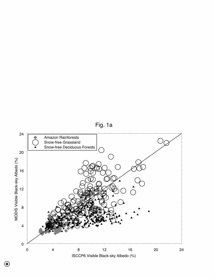
0 4 8 12 16 20 24ISCCP6 Visible Black-sky Albedo (%)

0

4

8

12

16

20

24

MO

DIS

Visib

le B

lack

-sky

Alb

edo

(%)

Amazon RainforestsSnow-free GrasslandSnow-free Deciduous Forests

Fig. 1a

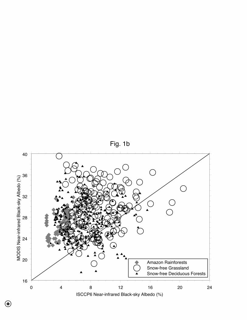
0 4 8 12 16 20 24ISCCP6 Near-infrared Black-sky Albedo (%)

16

20

24

28

32

36

40

MO

DIS

Near

-infra

red

Blac

k-sk

y Al

bedo

(%)

Amazon RainforestsSnow-free GrasslandSnow-free Deciduous Forests

Fig. 1b

0 4 8 12 16 20 24ISCCP6 Total SW Black-sky Albedo (%)

8

12

16

20

24

28

32

MO

DIS

Tota

l SW

Bla

ck-s

ky A

lbed

o (%

)

Amazon RainforestsSnow-free GrasslandSnow-free Deciduous Forests

Fig. 1c

0 10 20 30 40 50 60 70 80 90 100ISCCP6 Visible Black-sky Albedo (%)

0

10

20

30

40

50

60

70

80

90

100

MO

DIS

Visib

le B

lack

-sky

Alb

edo

(%)

Snow-covered GrasslandLand IceSea IceSahara Deserts

Fig. 1d

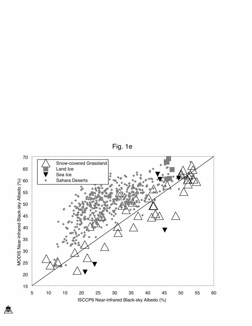
5 10 15 20 25 30 35 40 45 50 55 60ISCCP6 Near-infrared Black-sky Albedo (%)

15

20

25

30

35

40

45

50

55

60

65

70

MO

DIS

Near

-infra

red

Blac

k-sk

y Al

bedo

(%)

Snow-covered GrasslandLand IceSea IceSahara Deserts

Fig. 1e

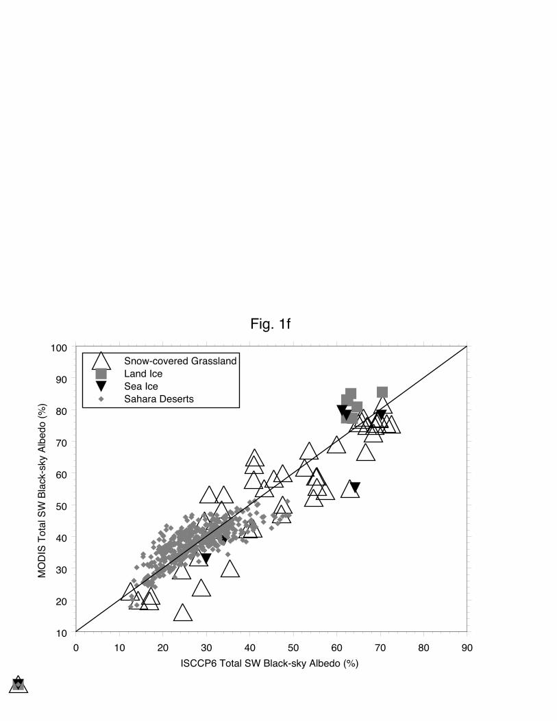
0 10 20 30 40 50 60 70 80 90ISCCP6 Total SW Black-sky Albedo (%)

10

20

30

40

50

60

70

80

90

100

MO

DIS

Tota

l SW

Bla

ck-s

ky A

lbed

o (%

)

Snow-covered GrasslandLand IceSea IceSahara Deserts

Fig. 1f

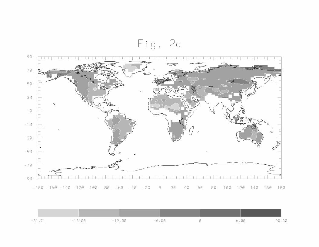
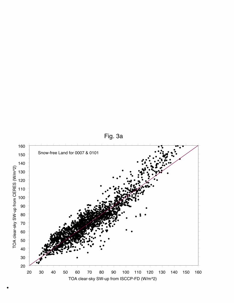
20 30 40 50 60 70 80 90 100 110 120 130 140 150 160TOA clear-sky SW-up from ISCCP-FD (W/m^2)

20

30

40

50

60

70

80

90

100

110

120

130

140

150

160

TOA

clear

-sky

SW

-up

from

CER

ES (W

/m^2

)

Fig. 3a

Snow-free Land for 0007 & 0101

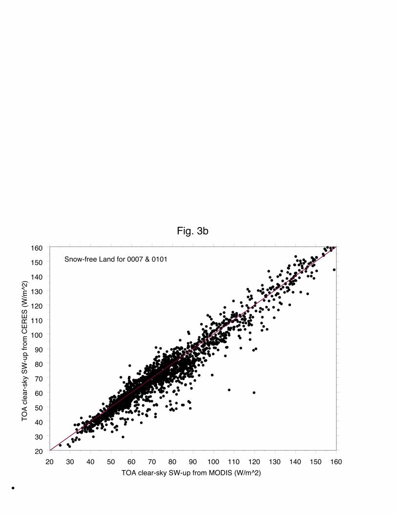
Snow-free Land for 0007 & 0101

20 30 40 50 60 70 80 90 100 110 120 130 140 150 160TOA clear-sky SW-up from MODIS (W/m^2)

20

30

40

50

60

70

80

90

100

110

120

130

140

150

160

TOA

clear

-sky

SW

-up

from

CER

ES (W

/m^2

)

Fig. 3b

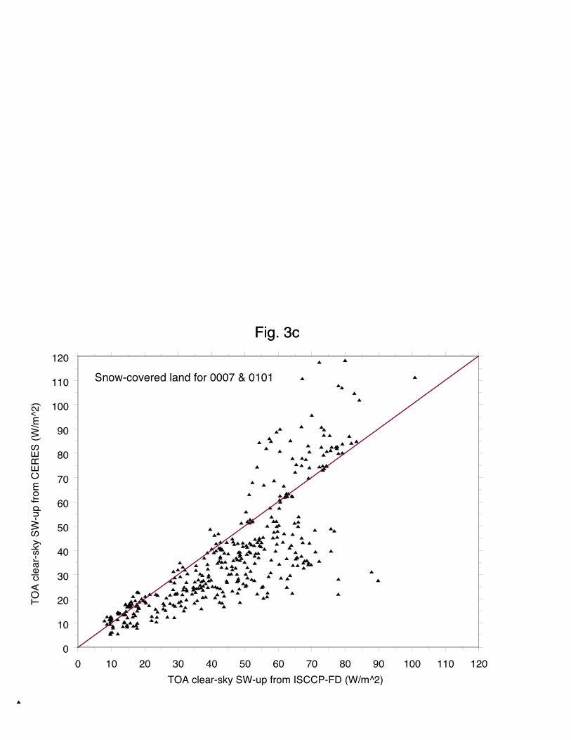
0 10 20 30 40 50 60 70 80 90 100 110 120TOA clear-sky SW-up from ISCCP-FD (W/m^2)

0

10

20

30

40

50

60

70

80

90

100

110

120

TOA

clear

-sky

SW

-up

from

CER

ES (W

/m^2

)

Snow-covered land for 0007 & 0101

Fig. 3cFig. 3c

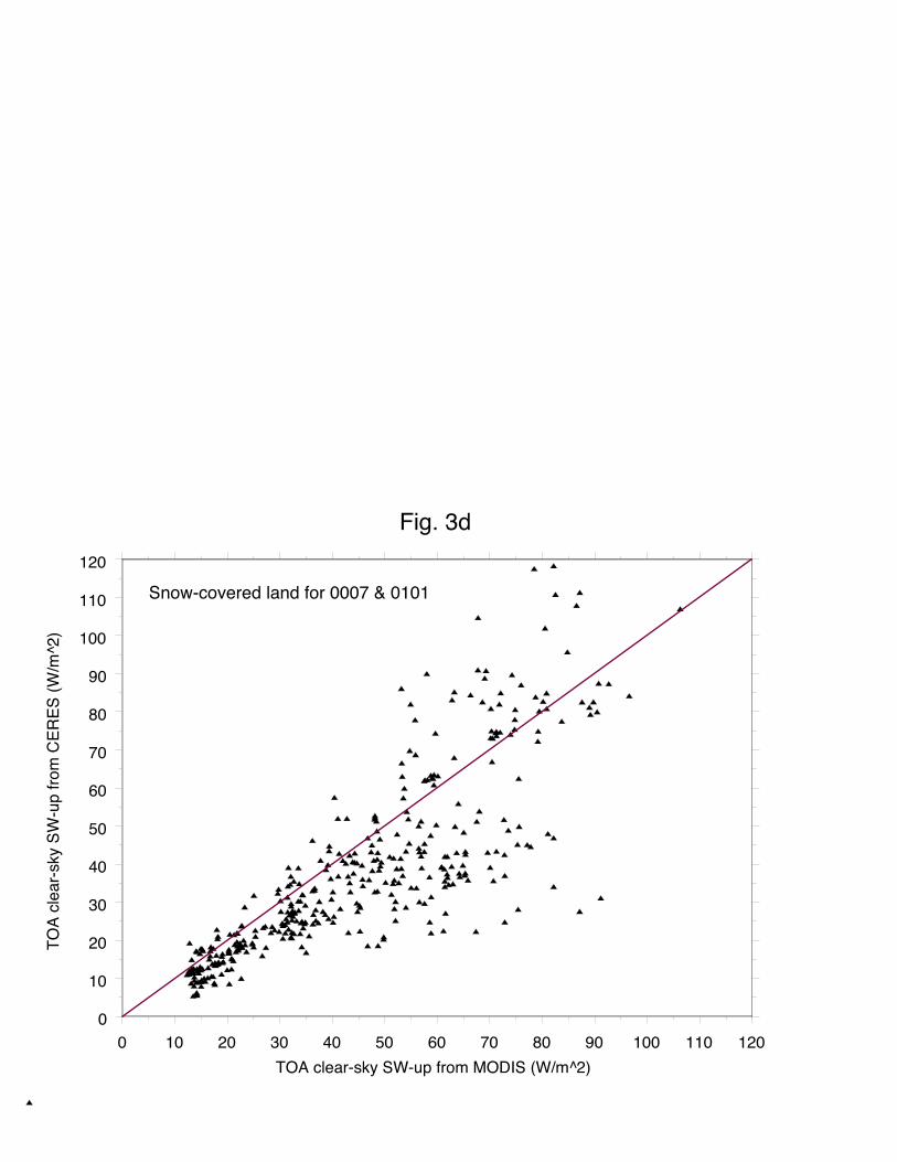
0 10 20 30 40 50 60 70 80 90 100 110 120TOA clear-sky SW-up from MODIS (W/m^2)

0

10

20

30

40

50

60

70

80

90

100

110

120

TOA

clear

-sky

SW

-up

from

CER

ES (W

/m^2

)

Snow-covered land for 0007 & 0101

Fig. 3d

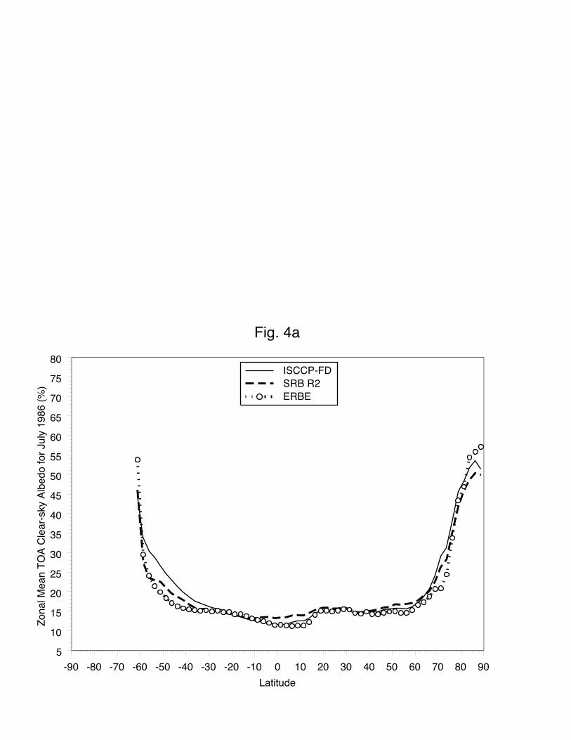
-90 -80 -70 -60 -50 -40 -30 -20 -10 0 10 20 30 40 50 60 70 80 90Latitude

5

10

15

20

25

30

35

40

45

50

55

60

65

70

75

80

Zona

l Mea

n TO

A Cl

ear-s

ky A

lbed

o fo

r Jul

y 19

86 (%

)

ISCCP-FDSRB R2ERBE

Fig. 4a

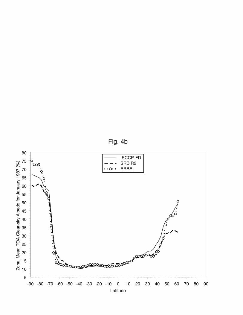
-90 -80 -70 -60 -50 -40 -30 -20 -10 0 10 20 30 40 50 60 70 80 90Latitude

5

10

15

20

25

30

35

40

45

50

55

60

65

70

75

80

Zona

l Mea

n TO

A Cl

ear-s

ky A

lbed

o fo

r Jan

uary

198

7 (%

) ISCCP-FDSRB R2ERBE

Fig. 4b

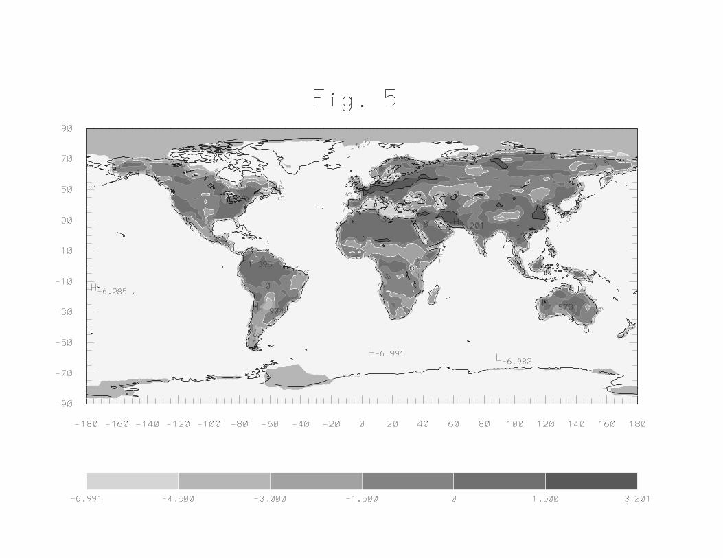
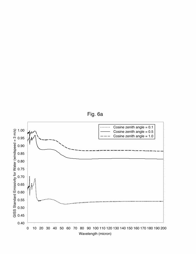
0 10 20 30 40 50 60 70 80 90 100 110 120 130 140 150 160 170 180 190 200Wavelength (micron)

0.40

0.45

0.50

0.55

0.60

0.65

0.70

0.75

0.80

0.85

0.90

0.95

1.00

GIS

S St

anda

rd E

miss

ivity

for W

ater

(win

dspe

ed =

3 m

/s) Cosine zenith angle = 0.1

Cosine zenith angle = 0.5Cosine zenith angle = 1.0

Fig. 6a

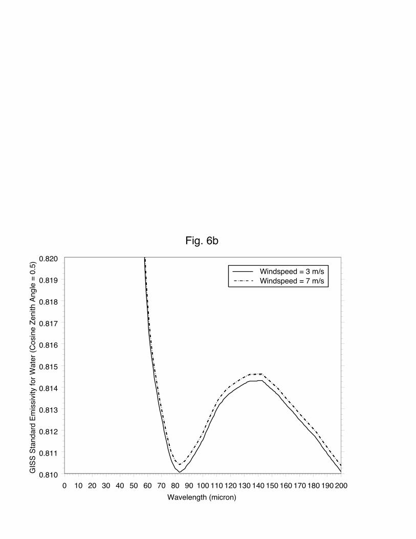
0 10 20 30 40 50 60 70 80 90 100 110 120 130 140 150 160 170 180 190 200Wavelength (micron)

0.810

0.811

0.812

0.813

0.814

0.815

0.816

0.817

0.818

0.819

0.820

GIS

S St

anda

rd E

miss

ivity

for W

ater

(Cos

ine

Zeni

th A

ngle

= 0

.5)

Windspeed = 3 m/sWindspeed = 7 m/s

Fig. 6b

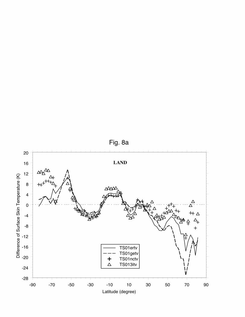
-90 -70 -50 -30 -10 10 30 50 70 90Latitude (degree)

-28

-24

-20

-16

-12

-8

-4

0

4

8

12

16

20

Diffe

renc

e of

Sur

face

Skin

Tem

pera

ture

(K)

TS01ertvTS01getvTS01nctvTS013itv

LAND

Fig. 8a

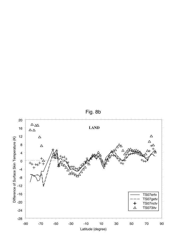
-90 -70 -50 -30 -10 10 30 50 70 90Latitude (degree)

-28

-24

-20

-16

-12

-8

-4

0

4

8

12

16

20

Diffe

renc

e of

Sur

face

Skin

Tem

pera

ture

(K)

TS07ertvTS07getvTS07nctvTS073itv

LAND

Fig. 8b

-90 -70 -50 -30 -10 10 30 50 70 90Latitude (degree)

-18

-16

-14

-12

-10

-8

-6

-4

-2

0

2

4

6

8

10

12

Diffe

renc

e of

Sur

face

Skin

Tem

pera

ture

(K)

TS01ertvTS01getvTS01nctvTS013itv

Fig. 8c

OCEAN

-90 -70 -50 -30 -10 10 30 50 70 90Latitude (degree)

-18

-16

-14

-12

-10

-8

-6

-4

-2

0

2

4

6

8

10

12

Diffe

renc

e of

Sur

face

Skin

Tem

pera

ture

(K)

TS07ertvTS07getvTS07nctvTS073itv

Fig. 8d

OCEAN

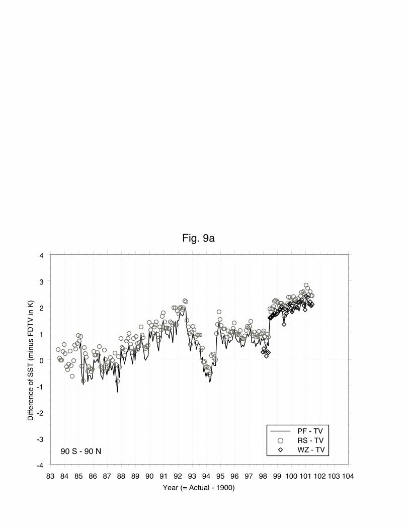
83 84 85 86 87 88 89 90 91 92 93 94 95 96 97 98 99 100 101 102 103 104Year (= Actual - 1900)

-4

-3

-2

-1

0

1

2

3

4

Diffe

renc

e of

SST

(min

us F

DTV

in K

)

90 S - 90 N

PF - TVRS - TVWZ - TV

Fig. 9a

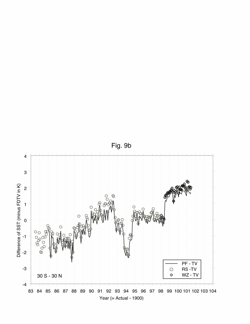
83 84 85 86 87 88 89 90 91 92 93 94 95 96 97 98 99 100 101 102 103 104Year (= Actual - 1900)

-4

-3

-2

-1

0

1

2

3

4

Diffe

renc

e of

SST

(min

us F

DTV

in K

)

30 S - 30 N

PF - TVRS -TVWZ - TV

Fig. 9b