c marine engineering and management comem

ERASMUS MUNDUS MSC PROGRAMME

COASTAL AND MARINE ENGINEERING AND MANAGEMENT COMEM

COMPOSITE SEAWALL FOR WAVE ENERGY CONVERSION

Delft University of Technology June 2010

Abul Bashar Mohammed Khan Mozahedy

1550284

The Erasmus Mundus MSc Coastal and Marine Engineering and Management is an integrated programme organized by five European partner institutions, coordinated by Delft University of Technology (TU Delft). The joint study programme of 120 ECTS credits (two years full-time) has been obtained at three of the five CoMEM partner institutions: Norges Teknisk- Naturvitenskapelige Universitet (NTNU) Trondheim, Norway Technische Universiteit (TU) Delft, The Netherlands City University London, Great Britain Universitat Politècnica de Catalunya (UPC), Barcelona, Spain University of Southampton, Southampton, Great Britain The first year consists of the first and second semesters of 30 ECTS each, spent at NTNU, Trondheim and Delft University of Technology respectively. The second year allows for specialization in three subjects and during the third semester courses are taken with a focus on advanced topics in the selected area of specialization: Engineering Management Environment In the fourth and final semester an MSc project and thesis have to be completed. The two year CoMEM programme leads to three officially recognized MSc diploma certificates. These will be issued by the three universities which have been attended by the student. The transcripts issued with the MSc Diploma Certificate of each university include grades/marks for each subject. A complete overview of subjects and ECTS credits is included in the Diploma Supplement, as received from the CoMEM coordinating university, Delft University of Technology (TU Delft). Information regarding the CoMEM programme can be obtained from the programme coordinator and director Prof. Dr. Ir. Marcel J.F. Stive Delft University of Technology Faculty of Civil Engineering and geosciences P.O. Box 5048 2600 GA Delft The Netherlands

FACULTY OF ENGINEERING, SCIENCE AND MATHEMATICS

SCHOOL OF CIVIL ENGINEERING AND THE ENVIRONMENT

Composite seawall for wave energy conversion


June, 2010

i

UNIVERSITY OF SOUTHAMPTON

FACULTY OF ENGINEERING, SCIENCE AND MATHEMATICS

SCHOOL OF CIVIL ENGINEERING AND THE ENVIRONMENT

Composite seawall for wave energy conversion


“A dissertation submitted to the School of Civil Engineering and the Environment, University of

Southampton in partial fulfilment of the degree of M.Sc. in Coastal and Marine Engineering and

Management (CoMEM) by instructional course.”

June, 2010

ii

Summary

Detrimental impacts of fossil fuels and its foreseen scarcity are encouraging research for the

development of the renewable energy as alternatives. A newly developed composite seawall

concept could be a vitally important technique for wave energy conversion. A 3-D model of

composite seawall has been simulated to comprehend its hydraulic performance.

Composite seawall is a dual-purpose overtopping type of coastal shoreline device and wave

energy conversion is considered as by-product of the seawall. Overtopped water generates

hydraulic head convertible to electricity by means of low head hydro-power generator.

A 3-D physical model of composite seawall has been developed and tested for both normal and

oblique waves in this study. Fraude scale laws (geometric scale 1:50) are followed in the model

scaling. Total 72 simulations are conducted, and overtopping and hydraulic power generated at

the crest of the ramp of the composite seawall for each simulated wave parameters are

recorded. Hydraulic performances are measured based on the input wave parameters and

results. Wave breaker screen is also modeled and tested (by 12 simulations) to measure its

suitability as outfall.

Results show that maximum achievable hydraulic efficiency of the composite seawall is about

33.6 % and average hydraulic efficiencies are about 26.6%, 18.6%, 15.9% and 11.1% for the

freeboard of 0.5 m, 1.0 m, 1.5 m and 2.0 m respectively. Hydraulic performance decreases for

oblique wave approaches. Average hydraulic efficiency of a composite seawall (having 1.0 m

freeboard) is about 20% in case of 1.0 m tidal variation. Composite seawall is not suitable option

for high tidal variations and low wave heights. Wave breaker screen is a suitable outfall option

but it decreases hydraulic head generated in the composite sea walls up to 12.5%.

Composite sea walls for wave energy extraction could be suitable option in such a remote place

such as Islands, where conventional energy supply would be highly expensive and rarely

possible.

iii

Acknowledgement

The author wishes to express profound thanks to Dr. Gerald Muller, Senior Lecturer, School of

Civil Engineering and the Environment, University of Southampton for kindly supervising of such

an interesting and innovating research study. The author is indebted to him for the time, efforts

and supports, which he has given in the whole process of the research.

The author thanks to Mr. Rhys Jenkins for his valuable guidance and supports during the

physical modeling in the Hydraulics Laboratory.

The author thanks to all officials and PhD students of this University, who has helped in the

research study.

The author expresses thanks to relatives and friends for their supports and blessing.


Southampton, United Kingdom

iv

Contents

Summary ii Acknowledgement iii Contents iv List of figures vi List of tables vii List of abbreviations viii Chapter I: Introduction 1

1.1 Background 1 1.2 Objectives of the study 2 1.3 Scopes of the study 2 1.4 Methodology 2 Chapter II: Literature review 3

2.1 Wave energy 3 2.2 Linear wave theory 3 2.3 Wave transformations 6 2.4 Wave overtopping 8

2.5 Wave energy conversion 10 2.6 Overtopping WECs: Wave dragon and SSG 12 2.7 Composite seawall 14 2.8 Hydrostatic Pressure Wheel (HPW) 15 2.9 Physical modeling of coastal structures 17 2.10 Scaling and similitude 18 2.11 Scale effects 20 2.12 Laboratory effects 21 2.13 Outfall 21

Chapter III: Theory and Experiments 24

3.1 Experimental setup 24 3.2 Scaling of parameters 26 3.3 Wave overtopping prediction 27 3.4 Overtopping performance 29 3.5 Performance comparison with oblique waves 30

v

3.6 Power performance 30 3.7 Performance optimization against tidal variation 31

3.8 Outfall designing 31 3.9 Observations 32

Chapter IV: Results and discussion 33

4.1 Overtopping performance with normal waves 33 4.2 Hydraulic performance with normal waves 37 4.3 Overtopping performance at oblique waves 40 4.4 Hydraulic performance at oblique waves 42 4.5 Performance optimization with tidal variations 48 4.6 Outfall design 50 4.7 Simple experimental observations 52 4.8 Market potential of composite seawall for WECs 53

Chapter V: Conclusion 54

5.1 Conclusions 54 5.2 Further study 55

References 56 Appendix I: Sample calculations of wave analysis and overtopping 60 Appendix II: Sample prediction calculations of overtopping 61 Appendix III: Sample calculations of hydraulic performance 62 Appendix IV: Sample calculations of outfall design: wave breaker screen 63 Appendix V: Sketch of the designed outfall: wave breaker screen 64

vi

List of figures Figure 2.1: Ocean waves 3 Figure 2.2: Basic parameters of a monochromatic propagating wave 4 Figure 2.3: Wave reflection and standing waves 8 Figure 2.4: Overtopping of sloped coastal structures 9 Figure 2.5: Green and White water overtopping 9 Figure 2.6: Recently developed WECs 12 Figure 2.7: Wave dragon and its working principle 13 Figure 2.8: SSG and its working principle 13 Figure 2.9: High mound composite seawall, constructed at Mori port in Japan 14 Figure 2.10: Composite seawall for energy conversion 15 Figure 2.11: Schematic diagram of HPW and its theoretical efficiency 16 Figure 2.12: Submarine outfall system 22 Figure 2.13: flushing gate and its working principle 22 Figure 3.1: Composite seawall model of 1:50 scale 24 Figure 3.2: Wave tank 25 Figure 3.3: Model of the outfall 32 Figure 4.1: Measured overtopping with wave heights at different freeboard conditions 35 Figure 4.2: Comparisons of measured overtopping with predictions (Freeboard 1.0 m) 36 Figure 4.3: Comparisons of measured overtopping with predictions (Freeboard 1.5 m) 36 Figure 4.4: Hydraulic performance at significant wave height 39 Figure 4.5: Hydraulic efficiency of the seawall at significant wave heights 39 Figure 4.4: Overtopping at different angles (Freeboard 1.0 meter) 41 Figure 4.5: Overtopping at different angles (Freeboard 1.5 meters) 41 Figure 4.6: Wave period dependence of overtopping (Freeboard 1.5 meters) 42 Figure 4.7: Hydraulic power at different angles (Freeboard 1.0 meter) 46 Figure 4.8: Hydraulic power at different angles (Freeboard 1.5 meters) 46 Figure 4.9: Hydraulic efficiency at different angles (Freeboard 1.0 meter) 47 Figure 4.10: Hydraulic efficiency at different angles (Freeboard 1.5 meters) 47 Figure 4.11: Hydraulic performance with Hs/Rc ratios 49 Figure 4.12: Funnelling effect at oblique waves of 300 53

vii

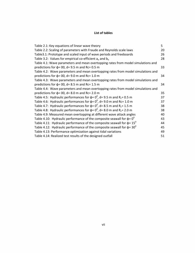
List of tables Table 2.1: Key equations of linear wave theory 5 Table 2.2: Scaling of parameters with Fraude and Reynolds scale laws 20 Table3.1: Prototype and scaled input of wave periods and freeboards 26 Table 3.2: Values for empirical co-efficient ao and bo 28 Table 4.1: Wave parameters and mean overtopping rates from model simulations and predictions for φ= 00, d= 9.5 m and Rc= 0.5 m 33 Table 4.2: Wave parameters and mean overtopping rates from model simulations and predictions for φ= 00, d= 9.0 m and Rc= 1.0 m 34 Table 4.3: Wave parameters and mean overtopping rates from model simulations and predictions for φ= 00, d= 8.5 m and Rc= 1.5 m 34 Table 4.4: Wave parameters and mean overtopping rates from model simulations and predictions for φ= 00, d= 8.0 m and Rc= 2.0 m 35 Table 4.5: Hydraulic performances for φ= 00, d= 9.5 m and Rc= 0.5 m 37 Table 4.6: Hydraulic performances for φ= 00, d= 9.0 m and Rc= 1.0 m 37 Table 4.7: Hydraulic performances for φ= 00, d= 8.5 m and Rc= 1.5 m 38 Table 4.8: Hydraulic performances for φ= 00, d= 8.0 m and Rc= 2.0 m 38 Table 4.9: Measured mean overtopping at different wave attack angles 40 Table 4.10: Hydraulic performance of the composite seawall for φ= 00 43 Table 4.11: Hydraulic performance of the composite seawall for φ= 150 44 Table 4.12: Hydraulic performance of the composite seawall for φ= 300 45 Table 4.13: Performance optimization against tidal variations 49 Table 4.14: Realized test results of the designed outfall 51

viii

List of abbreviations HPW Hydrostatic Pressure Wheel HHWL Higher High Water Level HWL High Water Level LLWL Lower Low Water Level LWL Low Water Level MWL Mean Water Level OWC Oscillating Water Column SSG Sea Slot-cone Generator UK United Kingdom WEC Wave Energy Converter 2-D Two Dimensional 3-D Three Dimensional

1

Chapter I

Introduction

1.1 Background

Carbon emission to the atmosphere causes global warming. Uses of fossil fuel have brought

detrimental changes to the global climate during last decades. Moreover, world reserve of the

fossil fuel (mainly oil and gas) is depleting at an accelerating rate due to tremendous

dependence on them. Hence, development of renewable energies is a growing demand as an

alternative source of energy.

Among the renewable energies, wave energy is vitally important, although considerable

progress is not achieved yet. Sometimes, composite sea walls consist of obstacles in front of it to

enhance wave energy dissipation and to reduce wave loadings and related damages. This type

of composite seawall is constructed recently at Mori port in Japan and research shows that 15%

construction cost is reduced in the composite seawall compared to the conventional Japanese

seawall (Mori, 2008).

A composite seawall with narrow reservoir along its length has been developed at Southampton

University to convert wave energy into potential energy. Muller (2009) has pointed out that

main advantage of this seawall is its cost-effectiveness, as it is a dual purpose structure,

providing protection and energy generation. Water is collected in the reservoir through

overtopping to create head difference. A Wave Energy Converter (WEC) has been developed

using Hydrostatic Pressure Wheel (HPW), which is found potentially very effective for very low

head differences.

Muller (2009) described the HPW as a very simple and cost-effective hydropower converter

which can tolerate large variations in flow rate. The combination of a very low head (less than 1

meter) hydropower source with this converter could result in an overall cost-effective system.

Maravelakis (2009) measured efficiencies of the composite seawall for WEC in 2-D physical

model tests and found that maximum hydraulic efficiencies are about 32% in 1/50 scale model

and about 28% in 1/23 scale model.

Sea states are random and obviously it is three dimensional (3-D) in nature. Hydraulic

performance mainly depends on the collection of water in the reservoir. Water collection

depends on the wave height and its consistency with time. 3-D physical model testing will lead

2

to determine hydraulic performance of the system. Parallel waves and oblique waves may give

different results in collecting water, which will be compared in this project.

The outfall of the composite seawall is very important as the HPW will be installed at outlet. It

should be free from wave actions to ensure smooth functioning of the HPW and to have easy

passage of water return to the sea. Suitable outfall designs will be developed and tested in this

project, considering various factors involved such as random wave attack and fluctuations of the

water surface.

1.2 Objectives of the study

The aims of the research study are to develop realistic performance prediction tools and design

details for composite seawalls as WEC. Specific objectives of the study are as follows:

1. Hydraulic performance of a composite seawall in 3-D physical model.

2. Performance comparison for oblique waves with regular waves.

3. Detailing of suitable outlets based on model study results.

1.3 Scope of the study

Main scopes of the study are the availability of physical modelling facilities in the hydraulic

laboratory at Southampton University. The facilities include 3-D wave basin, wave generating

and monitoring devices and composite seawall (scale 1:50).

1.4 Methodology A 3-D physical model of composite seawall will be constructed in the 3-D wave basin of the

hydraulic laboratory. Waves will be produced by wave generating devices at different angles and

magnitudes. Water will be collected in the reservoir of the composite seawall through

overtopping. The model will be tested in the laboratory to determine hydraulic performance of

the system. Model results will be converted into the prototype results for analysis and better

understanding. Suitable outfall will be designed and tested in the model.

3

Chapter II

Literature Review

2.1 Wave energy

Ocean waves are caused by the wind stress while wind blows over the water surface. Waves are

sinusoidal fluctuations (ups and downs) of the water surface in the sea. Wave gets energy from

wind stress and becomes a powerful source of renewable energy.

Figure 2.1: Ocean waves (OCS, 2010 and Muller, 2009)

2.2 Linear Wave Theory

Among the regular wave theories, linear wave theory, proposed by Sir George Airy (1801-1892)

for two dimensional and freely propagating periodic gravity waves, is appropriate only for waves

of small steepness (small H/L). Steeper waves become progressively more non-linear as the

limiting condition (Chaplin, 2009). Linear wave theory is used in this thesis to calculate and

analyze wave parameters as it is easy to apply and extensively used in wave analysis. Important

and relevant literary descriptions of linear wave theory are taken from Chaplin (2009). Basic

parameters of a monochromatic propagating wave are shown in the figure 2.2.

4

Figure 2.2: Basic parameters of a monochromatic propagating wave (Chaplin, 2009)

In the above figure 2.2, the reference frame (x, z) is fixed in space and on the free surface, the

value of z is a function of x and t so that z= η(x, t). Wave parameters are discussed as follows:

L= Wave length, is the linear distance between two successive identical points (for example

crests or troughs) on the wave.

T= Wave period, time difference between two successive identical points (wave length).

H= Wave height, vertical distance between two successive crest and trough.

d= Water depth, from the Mean Water Level (MWL).

f= Wave frequency= 1/T (in Hz).

ω= Wave frequency = 2π/T (in radians/sec).

k= Wave number= 2π/L

a= Wave amplitude= H/2.

H/L= Wave steepness.

d/L= Relative depth.

C=Wave celerity= L/T.

At any arbitrary point, the velocity of the water particle has both horizontal and vertical

components (u, w), which are function of x, z and t. Shape of the water particle movement

depends on the relative depth (d/L) of water. This shape is circular in deep water and diminishes

5

along the depth, whereas it becomes horizontally elliptical in shallow water and diminishes

along depth until it touches the bottom. Conditions of deep and shallow waters are as follows:

Deep water depth when d/L>1/2.

Shallow water depth when d/L<1/20.

Intermediate water depth when 1/20≤d/L≤1/2.

Basics assumptions (and conditions for solution) of linear wave theory:

Wave steepness (H/L) is small.

Surface tension is unimportant and negligible.

The fluid is homogeneous, incompressible and fluid viscosity is negligible.

The flow is irrotational. Shearing forces are neglected.

Sea bottom is impermeable meaning vertical particle velocity at the bottom is zero.

Pressure at the free surface is atmospheric.

Motion of the free surface is compatible with motion of the water.

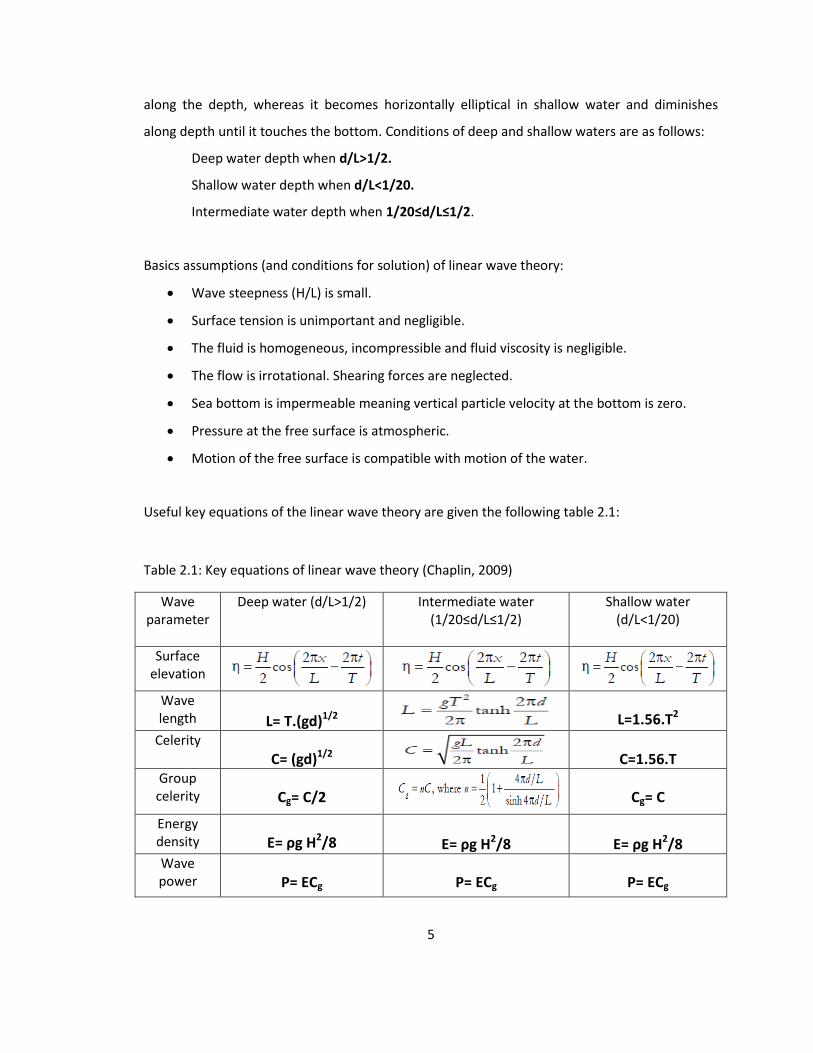
Useful key equations of the linear wave theory are given the following table 2.1:

Table 2.1: Key equations of linear wave theory (Chaplin, 2009)

Wave parameter

Deep water (d/L>1/2)

Intermediate water (1/20≤d/L≤1/2)

Shallow water (d/L<1/20)

Surface elevation

Wave length

L= T.(gd)1/2

L=1.56.T2

Celerity

C= (gd)1/2

C=1.56.T

Group celerity

Cg= C/2

Cg= C

Energy density

E= ρg H2/8

E= ρg H2/8

E= ρg H2/8

Wave power

P= ECg

P= ECg

P= ECg

6

In the table 2.1,

ρ= Density of water

g= Gravitational acceleration

C= Celerity or velocity of wave

Cg= Group velocity

E= Energy density, average energy per unit area of sea surface

P= Power propagated by wave per unit width

(Other wave parameters are defined in the previous paragraphs)

2.3 Wave Transformations

Wave parameters change due to changes in water depth, seabed geometry and contours while

it travels towards the shore. Superimposition of reflected and incidence waves and any

obstructions on its way also cause changes in wave parameters. Four important causes and their

consequences (based on Chaplin, 2009) are described below for better understanding of the

physical modelling effects.

Shoaling

Wave shoaling is the changes in wave length and wave height due to reducing water

depth (assuming that wave period (T) and wave power (P) remain unchanged), when the

wave crests are parallel to the seabed contours while travel towards the shore. Generally

wave height increases when wave crest travels from deep water to shallow water.

Shoaling co-efficient (KS) relates the changes in wave height in the following way.

(2.1)

Where

KS is shoaling co-efficient

H0 is wave height in deep water

H is wave height at shallow water depth (d)

L is the wave length at shallow water depth (d)

7

Refraction

When wave crest travels at an oblique angle with the seabed contours, it tries to be

parallel and hence change occurs in wave height (assuming no power travels sideways

along the crest). Eventually refraction reduces wave height while travelling towards the

shore. Refraction co-efficient (KR) relates changes in wave heights and angles of approach

in the following way.

(2.2)

Where

KR is refraction co-efficient

H0 is wave height in deep water depth

α0 is angle of wave approach in deep water depth

H is wave height at shallow water depth (d)

α is angle of wave approach in shallow water depth (d)

Diffraction

When there are rapid changes in the wave height along the wave crests, power travels

sideways. This phenomenon is called wave diffraction. Diffraction happens when wave

encounters obstructions (like breakwater, groin, spar etc) in its way to the shore.

Reflection

When wave reflects upon vertical or inclined wall, the reflected wave collides with the

incoming incidence wave and superimpose together to form a new wave changing wave

length and height. The newly formed wave is standing wave. Phenomena of wave

reflection and standing waves are shown in the figure 2.3.

8

Figure 2.3: Wave reflection and standing waves (Chaplin, 2009)

Reflection co-efficient (Rreff) is as follows:

(2.3)

Where

Hmax is maximum wave height at the anti-node of the standing wave

Hmin is minimum wave height at the node of the standing wave

2.4 Wave overtopping

The main purpose of the coastal structures (seawall, dike, revetment, breakwater etc) is to

protect land and properties from the wave attack, still storm waves cause overtopping of these

structures and endanger lives and coastal infrastructures. Lots of research and experimental

investigation has been done during the last 50 years to understand overtopping phenomena and

guidelines has been derived to design coastal structures in order to minimise overtopping

damages. Concept of the coastal wave overtopping is shown in the figure 2.4.

Wave reflection and superimposition

Perfect standing wave

Imperfect standing wave

9

Figure 2.4: Overtopping of sloped coastal structures (EurOtop, 2007 and HR Wallingford, 2010)

During stormy conditions, wave approaches up the face of a sloped structure and passes over

the crest as like as a sheet of water, which is called green water overtopping. White water

overtopping or impulsive overtopping occurs when waves hit the face of the coastal structures

(like seawall) with tremendous pressure and mixed with air, then push this aerated water

vertically up of the structure. These two types of overtopping are shown in the figure 2.5.

Figure 2.5: Green and White water overtopping (Soliman, 2003 and Muller, 2009)

10

Overtopping discharges vary up to several orders of magnitude from one wave to another under

random wave conditions, meaning that it is a non-linear function of wave height and wave

period. Overtopping depends not only on wave parameters such as wave height, wave period,

wave length, water level but also on geometric layout and material properties of the structure

(Soliman, 2003).

However many researchers have been trying to develop methods and formulas in order to

predict overtopping discharges of coastal structures on certain possible conditions. These

prediction formulas are widely varying and results in wide variations.

Most of the prediction methods and formulas for mean overtopping rate are derived from

numerical and physical modelling in the laboratory facilities, which leads to develop empirical

relationship of overtopping discharge rate with wave parameters, basin geometry and material

properties of the structures. Renowned prediction methods and formals are derived by Owen

(1980, 1982), Brudbury and Allsop (1988), Pedersen and Burchartch (1992), Van der Meer and

Janssen (1995) and Goda (2000). All of the prediction formulas are derived for sloping coastal

structures (with or without rocked armour and crown wall) of more or less generally

impermeable, smooth or rough, straight or bermed sloped seabed geometry (ibid).

Moravelakis (2009) has found Owen (1980) to be unsuitable for the predictions of wave

overtopping over a composite seawall in 2-D wave basin and the prediction results by Van der

Meer and Janssen (1995) and Goda (2000) are more ordered than that of Owen (1980).

Among the above overtopping prediction formulas, Owen (1980) and Van der Meer and Janssen

(1995) are used to predict overtopping rates of the 3-D physical model in this thesis. Details of

these two prediction methods are described in the chapter III.

2.5 Wave energy conversion

Fossil fuel causes detrimental changes in the environment due to CO2 emissions. Moreover,

extensive use of fossil fuel is depleting rapidly the reserves of oil, coal and gas. Wave energy

conversion from renewable energy sources can be an alternative solution of the fossil fuel.

Among the renewable energy resources, exploitation of wave energy has been studied during

last decades, although considerable progress has not been achieved yet to compete with other

energy sources in the market. The main hindrance is that it is hardly possible to harness this

energy in economically viable way and convert it into electricity in large amounts. Kine (2005)

11

opined that there have been many attempts taken to harness the power of the ocean waves

over the last century, some showing limited short-term success but ultimately failing due to

technical or economic reasons. However, research continues to find out potential Wave Energy

Converter (WEC).

The already existed WECs can be distinguished into two categories: offshore WECs and shoreline

WECs. Offshore WECs are floating or submerged devices in deep water and anchored to the

seabed. Exploited energy is transferred to the shore by means of cables placed on the seabed.

Shoreline WECs are generally placed along the shore in shallow water and sometimes, can be

integrated with shoreline defenses (Maravelakis, 2009).

Offshore WECs may exploit huge potential of high wave energy density environment but they

suffer from extreme wave loadings, costly underwater cable connection for electricity

transmission, and difficulty in maintenance works. Shoreline WECs has relatively low potential of

wave energy as energy dissipated into the shallow waters. However, they may be cost-effective

due to low initial and maintenance costs and greater accessibility. Shoreline WECs can be

constructed in combination with shoreline defenses, which will eventually reduce production

costs too (ibid).

Among the WECs, Oscillating Water Column (OWC), Pelamis, Wave dragon, Oyster etc. are

prominent and recently developed devices (shown in the figure 2.6).

The existing WECs are differed in their working principles too. OWCs are chambers where water

level rises and falls with the wave fluctuations, causes air movement, which regulates air

turbine. Pelamis is a buoyant moored device developed by Ocean Power Delivery Ltd, which is

moved by the waves and energy is extracted from this motion. Oyster is a recent development

of WECs suitable in shallow water depth and still under research (ibid).

12

Figure 2.6: Recently developed WECs (Maravelakis, 2009 and Muller, 2009)

2.6 Overtopping WECs: Wave dragon and SSG

Overtopping devices are water reservoir, which collect water through wave overtopping and

generate potential hydraulic head. This hydraulic head drives a turbine to produce electricity.

Wave dragon is an overtopping device, which is usually installed in offshore. Waves run over the

ramp of the device and the water is stored in a reservoir. As more water enters the reservoir, an

equal amount of water is forced out through the turbine in the centre, causing it to rotate and

generate electric power (Kine, 2005). A simple wave dragon and its working principle are shown

in the figure 2.7.

OWC

OWC

Pelamis

Oyster

13

Figure 2.7: Wave dragon and its working principle (Wave dragon, 2005)

Sea Slot-cone Generator (SSG) is another overtopping device, which is placed along the shore

and integrated with shoreline defence systems like breakwater or rock cliff. There are multiple

reservoirs placed on top of each other, in which water from incoming waves is stored and then

runs multi-stage turbine to produce electricity. Multiple reservoirs utilize different heights of

water head and hence result in a high overall efficiency (Kofoed, 2005). A SSG and its working

principle are shown in the figure 2.8.

Figure 2.8: SSG and its working principle (Wave energy, 2005 and Leonard energy, 2007)

14

2.7 Composite seawall

Seawall is normally constructed along the coastline to protect land and property. However,

extreme waves cause overtopping of the seawall and endanger lives and properties during

storm and hence seawall has been gone through several modifications such as curved top etc. in

order to minimise overtopping. Recently a high mound composite seawall has been developed

and constructed at Mori port, Japan. Research shows that 15% construction cost is reduced in

the composite seawall compared to the conventional Japanese seawall (Mori, 2008). This

composite seawall has an armoured slope and a curtain of vertical piles in the front of the actual

seawall. The curtain dissipates wave energy and therefore, it reduces wave loads on the seawall.

A sketch composite seawall is shown in the figure 2.9.

Figure 2.9: High mound composite seawall, constructed at Mori port in Japan (Mori, 2008).

Southampton University, UK is currently developing an overtopping type composite seawall for

wave energy conversion. The curtain is replaced by an impermeable ramp to create a water

reservoir, which is shown in the figure 2.10. Overtopping water is collected into the reservoir to

create hydraulic head for energy conversion. However the generated hydraulic head is very

small (about 1.0 meter), and hence Hydrostatic Pressure Wheel (HPW), a potentially very

effective converter for low head differences, has been developed in the hydraulic laboratory

(Muller, 2009).

15

Figure 2.10: Composite seawall for energy conversion (Muller, 2009)

Muller (2009) has pointed out main advantage of this seawall as its cost-effectiveness. It is a

dual purpose structure, providing coastal protection and energy generation, but it is

incompatible in the tidal coastal waters.

2.8 Hydrostatic Pressure Wheel (HPW)

Composite seawall creates hydraulic head difference in the order of 1.0 meter. Low head

hydropower converter is needed to exploit wave energy of overtopping type composite seawall

in a cost-effective way. Wave dragon and SSG use low head water Kaplan turbines, but it is

rarely considered as economically viable. Southampton University has developed a special type

of Hydrostatic Pressure Wheel (HPW), which is very effective in conversion of low head

differences (Muller, 2009).

HPW is usually installed at the end (outlet of the reservoir water) of the composite seawall and

the vanes rotate around its axis due to hydraulic head difference, when water passes through it.

A schematic diagram of HPW is shown in the figure 2.11.

16

Figure 2.11: Schematic diagram of HPW and its theoretical efficiency (Muller, 2009) In figure 2.11, HPW consists of a wheel of radius R, whose blades act as like as weir, creating

head difference (d1-d2). The hydrostatic pressure force (F=F1-F2) between upstream and

downstream acts on the blades. Muller (2009) assumes that blades move with the velocity of

the upstream water flow (v1). Hence, the power generated by the HPW is P= F × v1= (F1-F2) × v1.

Available Hydraulic power: (2.4)

Hydrostatic force on the blade: (2.5)

Hence theoretical efficiency of the HPW: (2.6)

(Muller, 2009)

For average wave heights of 1 m and a head difference of 0.9 m, a hydraulic power of 1.2 to 2

KW/m wall can be expected, provided that the energy converter has an estimated efficiency of

65% (hydraulic to electric), giving an overall efficiency of 17 to 28 % (Muller, 2009).

Maravelakis (2009) has measured maximum hydraulic efficiencies of the composite seawall in 2-

D physical model tests and found these efficiencies are about 32% in 1/50 scale model and

about 28% in 1/23 scale model.

17

2.9 Physical modelling of coastal structures

Physical modeling is an important tool of testing and validation for coastal engineers. Physical

models help to understand the complex hydrodynamic behavior of coastal structures, which

provide reliable and economic engineering design solutions (Hughes, 1993). Hughes (1993)

defines physical model as physical system reproduced at a reduced size so that the major

dominant forces acting on the system are represented in the model in the correct proportion to

the actual physical system.

Svendsen (1985) identifies three objectives of physical modeling in coastal engineering:

understanding insight of a physical phenomenon, verification of theoretical results and

obtaining measurements of complicated phenomena, which is inaccessible by theoretical

approaches. Dalrymple (1985), Le Mehaute (1976) and Kampphuis (1991), all have pointed out

major advantages and disadvantages of physical modeling study in coastal engineering. Main

advantages are no assumptions or omissions for simplification required, smaller size of the

model compared to the prototype makes easy acquisition of desired data, gives immediate

qualitative impression of the physical coastal processes and helps decision making process in

easy, quick and cost effective manner. Main disadvantages include scale effects and laboratory

effects during physical modeling study (Hughes, 1993).

Two types of physical modeling are found in the coastal engineering to study near shore coastal

physical characteristics. Fixed bed models are used to study propagation of waves and currents

in the coastal region. Fixed bed models can be either wave flume (2-D) or wave basin (3-D),

where evolution of waves can be studied over non-uniform bed geometry to observe physical

processes like refraction, diffraction, shoaling, breaking etc. Movable bed models are used to

study effects of water motion on deposition and transport of sediments. Physical modeling can

be either short term (hours to days) or long term (day to years), whereas short term modeling is

more practical to conduct in coastal engineering. Keulegan (1966) has pointed out two

requirements for success in physical modelling, which are equivalence between prototype and

model must be met to the extent possible under the constraints of the study and model data

must be properly interpreted in view of the known model shortcomings (ibid).

In the present study, fixed bed and short term physical model is used to study wave

propagations and to derive desired data of wave parameters and overtopping discharge.

18

2.10 Scaling and similitude

A prototype is the situation, which is being modelled, either in the same size or more often at

reduced scale. Scaling is fundamental in order to predict the processes of the prototype under

investigation. Scale ratio is the basis of correspondence tool of input parameters and results

between prototype and model. Le Mehaute (1976) has pointed out few criteria of a scale model.

Scale model must be exact in reproducing the phenomena under study, must be consistent in

producing results, must be sensitive and economical and must be of reasonable size within

reasonable time interval.

Scaling of a model in coastal engineering can be done by dimensional analysis. Hughes (1993)

has given details of methods of dimensional analysis in scaling of coastal physical models. Scale

ratio (Nx) is the ratio of the value of a parameter in the prototype (Xp) to the value of the same

parameter in the model (Xm). The reciprocal of this definition is also true.

Nx= Xp/Xm (2.7)

Similarity and similitude requirements should be met to reproduce a good model to a prototype.

Similitude is achieved when all the factors are in proportion between the prototype and the

model and the factors that are not in proportion should be so small as to be insignificant in the

process (Hughes, 1993).

There are three types of similarities in the hydraulic engineering: geometric similarity, kinematic

similarity and dynamic similarity. Geometric similarity means model is geometrically similar with

the prototype. Kinematic similarity means that all the motions (velocity, acceleration etc.) acting

on the model is similar with that of the prototype. Dynamic similarity means that the forces in

the model remain in the same relative (in proportion) magnitude as in the prototype (Hughes,

1993 and Dalrymple, 1985).

Dynamic similitude requires careful consideration of the forces acting on the system according

to their relative importance. Scale laws are simplified dynamic similitude of two interplayed

major forces. Scale criterion is the ratio between the inertia force to any other force, required to

be same in the model as in the prototype (Hughes, 1993).

19

Froude criterion: Froude number (Fr) is the square root of the ratio of inertia force to the gravity

force. Fraude number must be same in the model as in the prototype for dynamic similitude,

where gravity dominates over inertia. It is dimensionless and it can be simplified in the following

way:

(2.8)

Where, Fr= Froude number

u= Velocity

g= Gravitational acceleration

L= Length

Equation (2.8) is the Froude model criterion in which inertia is balanced by gravity, which is very

important for most flows with free surface. Hence, Froude criterion is widely used in the

hydraulic and coastal engineering model design (ibid).

Reynolds criterion: Reynolds number (Re) is the ratio of inertia force to the viscous force.

Reynolds number must be same in the model as in the prototype for dynamic similitude, if

viscous force dominates over the inertia. It is dimensionless and it can be simplified in the

following way:

(2.9)

Where, Re= Reynolds number

u= Velocity

ρ= Density of the fluid

μ= dynamic viscosity

L= Length

Forces related to the surface tension and elasticity are so small that they can be neglected from

the scaling a model in coastal engineering problems. Both Reynolds criterion and Froude

criterion are very important for designing the scaling of a specific model in coastal engineering,

but both can not be used at the same time. So it has to be determined which force between

gravity and viscous is dominating in the system (ibid).

20

Fraude criterion is used for the scaling of the model parameters in this study. The scaling of

several parameters is illustrated according to Fraude and Reynolds scale laws in the table 2.2.

Table 2.2: Scaling of parameters with Fraude and Reynolds scale laws (Hughes, 1993)

Parameter Unit Fraude scaling Reynolds scaling

Length m NL NL

Area m2 NA=NL2 NA=NL

2

Volume m3 NV=NL3 NV=NL

3

Time s Nt=NL1/2 Nt=NL

2/NV

Velocity m/s Nu=NL1/2 Nu=NV/NL

Overtopping rate m3/s/m Nq=NL3/2 Nq=NV

2.11 Scale effects

Hughes (1993) defines scale effects in the physical modelling as the differences between

prototype and model response that arise from the inevitably to simulate all the relevant forces

in the model at the proper scale dictated by the scaling (similitude) criteria. Le Mehaute (1976)

identifies scale effects as the error occurred due to unsatisfactory reproductions of some

phenomena in the smaller scale of the model compared to the prototype. Use of Fraude scale

law in the physical modelling incorrectly scaled forces related to viscosity and surface tension.

Similarly use of Reynolds scale law incorrectly scaled forces related to gravity and surface

tension in the model.

Le Metaute (1976) shows that scale effect of surface tension in wave propagation is less than 1%

if wave period and water depth are greater than 0.35 s and 2 cm respectively. Hughes (1993) has

pointed out that although surface tension produces insignificant scale effects, air entrainment in

breaking waves is affected since the size of the bubbles is determined by surface tension. The

content of the air bubbles is relatively small and less in number in the model.

Wave attenuation is the scale effect occurs by friction (both internal and bottom boundary

frictions) arising from viscosity of water due to neglecting Reynolds scale laws in hydraulic

physical modelling. Viscosity becomes important on wave run up and overtopping, which are

eventually decreased due to thinning of water layer in case of small overtopping rates (ibid).

21

2.12 Laboratory effects

Hughes (1993) defines laboratory effects as the differences occurred in the physical modelling

between prototype and model response due to limitations of the laboratory facilities such as

wave and flow generation techniques, solid model boundaries etc.

Incorrect reproduction of the prototype due to limitation of the model structure, geometry,

model boundaries etc. leads to laboratory effects in the physical modelling study. Sides of the

wave basin may affect the wave propagation by developing cross waves and wave damping

(Kortenhaus et al, 2005). Svendsen (1985) shows that a decrease of about 26% in wave height is

expected 30 m away from the wave maker in the flume.

Reflection of waves on the wave maker is another laboratory effect, which generates perfect or

imperfect standing waves and changes wave properties in the physical modelling results in the

flume or tank. Wave absorbers may reduce reflection and absorb unwanted reflected wave

energy (Hughes, 1993).

Use of tap water instead of seawater is another laboratory error in the coastal engineering

physical modelling study. Le Mehaute (1976) shows that 3% difference in density of water could

lead to 10-15% error on minimum weight of armour stones in the breakwater stability design

studies.

Influence of wind is an important laboratory effect of wave overtopping test, error occurs as

effects of wind transport are not considered in the coastal physical modelling study (kortenhaus

et al, 2005).

EurOtop (2007) noticed that position of the tray in the flume affect overtopping volume of

water, is another laboratory effects.

2.13 Outfall

Sea outfalls are normally used to discharge urban and industrial waste water and thermal water

from power plants. These outfalls are designed to facilitate mixing of the waste water over a

large volume of water in order to dilute waste and thermal water very quickly (Kumer, 1990).

Position of outfall and methods of discharging depends on types of the pollutants and their

processing (dilution, bio-degradation etc.) in the sea water. Based on pollutant types, physical

22

and environmental considerations, types of the receiving water body etc., outfalls can be

submarine, sub-surface or outlet at rivers, estuaries etc.

Submarine outfall: This type of outfall is usually suitable for thermal waste (also used for

industrial and urban) water disposal at deep sea or river bed. Waste water is conveyed by a

pipe, which is placed beneath seabed or riverbed. The main purpose is environmentally viable

disposal and proper mixing of waste water over a large water body (figure 2.12).

Figure 2.12: Submarine outfall system (Elmosa, 1989)

Flushing outlet: This outlet allows one way passage of the waste water discharge. This gate is

widely used for agricultural drainage against tidal variation. Gate becomes open during ebb tide

to allow drainage and remains close during flood tide (BWDB, 1988). Flushing outlet is also used

for urban sewerage outfalls at sea. A flushing gate and its working principle are shown in the

figure 2.13.

Figure 2.13: flushing gate and its working principle (ACU-GATE, 2003)

23

Wave breaker and breakwater: Breakwater is usually built to break waves and to keep water

calm inside the harbor. Revetments are used to break waves and to protect banks from erosion.

Rock, tetrapod, accropod, dolos, cube etc. are placed as armor units on the breakwaters or

revetments in single or multiple layers (Kamphuis, 2002). Mori (2008) used screen of vertical

piles in front of the seawall as a primary wave breaker. The curtain dissipates wave energy and

therefore, reduces wave loads on the seawall (figure 2.9).

24

Chapter III

Theory and Experiments

3.1 Experimental set up

Physical model study of a composite seawall for wave energy conversion has been conducted at

the Hydraulic Laboratory of the Southampton University, UK. A model of composite seawall

(about 1.2 m long) has been developed in a geometric scale of 1:50 for the present study, which

is shown in the figure 3.1.

Figure 3.1: Composite seawall model of 1:50 scale

The composite seawall was placed at a rectangular wave tank (length 3.0 m, width 1.5 m and

height 0.32 m), which is shown in the figure 3.2. The wave tank was equipped with wave peddle

and wave probes. The waves peddle and wave probes were connected with the computer

systems for wave generation and recording of wave parameters. Waves of specific parameters

were generated by the wave peddle systems. Software used in this system to generate waves

was ‘OWEL Drive and Collect’, which was a batch data taker and collect program. The wave

probes were used to collect water level fluctuations with time, which was measured through the

changes in the electric capacitance occurred due to water level fluctuations. The wave probes

25

were calibrated each day before going for model simulations. The software ‘COLLECT32’ was a

John’s 32-channel data collection program (1.01ASCII), which was used to calibrate the wave

probes to establish a relationship between water level fluctuations and changes in electric

capacitance. The data recordings were processed in tables and graphs to find out the realized

wave parameters with Microsoft Excel 2007. Wave parameters such as significant wave height,

wave period etc. were collected from the recording.

Figure 3.2: Wave tank

Simulations have been conducted for three positions of the composite seawall with respect to

the wave attack, which were normal wave attack (00 angle) and oblique wave attacks (150 and

300 angles). The study was conducted for unbroken waves only. The volume of water entered

into the water reservoir through overtopping was measured by water level gauge (area of the

reservoir was known) and mean overtopping rates were calculated. All model input data and

results were converted into prototype input data and results for analysis.

26

3.2 Scaling of parameters

Scaling of the model dimensions, wave parameters (height, period and wave length) and

overtopping rates were scaled following the Fraude scale laws (table 2.2). According to the

Fraude scale laws, geometric scale of the model was chosen as 1:50 for an imaginary prototype.

So, time scale and volumetric scale of the model became 1:7.07 and 1:125000 respectively.

Prototype and scaled input of wave periods (time scaling) and freeboards (geometric scaling) are

shown in the table 3.1. Composite seawall concepts for wave energy conversion are suitable

only for areas of low tidal ranges such as Mediterranean Sea and therefore, wave parameters

and freeboards are chosen accordingly.

Table3.1: Prototype and scaled input of wave periods and freeboards

Wave period Freeboard

Prototype, sec Model, sec Prototype, m Model, mm

4 0.57 0.5 10

6 0.85 1.0 20

8 1.13 1.5 30

2.0 40

Frequency of the wave peddle movements was calculated from the chosen wave period and

corresponding amplitude was set from observations of the model simulation results by trial and

error basis to set it for a specific significant wave height (Hs) generation.

Three wave heights were chosen to generate in simulation of each wave period, ranged from 0.5

to 2.5 m (10 to 50 mm in the model scale). But realized wave periods and significant wave

heights of the model simulations were collected from recording after each simulation. Wave

length has been calculated from the simulation results and water depth. All model results were

converted into full scale prototype results for analysis.

In each simulation, model overtopping rate (qm) was measured in m3/sec/m and then this was

converted into prototype overtopping rate (qp) according to Fraude scale laws (table 2.2) in the

following way.

qp= 501.5× qm (3.1)

27

3.3 Wave overtopping prediction

Overtopping of the 3-D physical model has been predicted by Owen (1980) and Van der Meer

and Jassen (1995) and compared with the measured overtopping rates. Aims of these formulas

are to minimise the overtopping of the sloped coastal structures while aims of composite

seawall are to maximise the overtopping in order to create hydraulic head as high as possible for

energy conversion. Both of the formulas predict wave overtopping rates at slopping coastal

structures, which are described below.

Owen (1980)

Owen (1980) proposes an overtopping formula of dimensionless overtopping rate (q) and

dimensionless freeboard (Rc) for simple smooth impermeable and simply sloped seawall. This

formula is originated based on extensive data set from model tests of sloped structures (Torch,

2004).

Owen (1980) overtopping formula reads (as in ibid):

(3.2)

Which is valid only when

(3.3)

Where

q is mean overtopping discharge rate per meter of width of the structure

Rc is the freeboard of the structure

Yr is surface roughness (Yr= 1.0 for smooth surface)

Tm is the mean wave period at the toe of the structure

g is gravitational acceleration

Hs is the significant wave height at the toe of the structure

In Owen (1980) method, wave height is considered as post breaking wave height. Besley (1999)

clarified the post breaking wave height as the significant wave height for correct overtopping

based on physical model tests (Soliman, 2003).

28

Goda (2000) suggested that the wave height in the near shore should be considered as the wave

height at the toe of the structure. Franco et al. (2009) measured the wave height in the field 220

meters seaward of the structure and in the corresponding scaled distance in the model studies

(Maravelakis, 2009).

ao and bo are two dimensionless empirically derived co-efficient in this methods, whose values

depend on the slope. Owen (1980) proposes values for different slopes, which are shown in the

table 3.2. Intermediate values were calculated by linear interpolation in this study.

Table 3.2: Values for empirical co-efficient ao and bo (Besley, 1999)

Slope of the seawall Values of ao Values of bo

1:1 0.00794 20.1

1:1.5 0.00884 19.9

1:2 0.00939 21.6

1:2.5 0.0103 24.5

1:3 0.0109 28.7

1:3.5 0.0112 34.1

1:4 0.0116 41.0

Besley (1999) (based on soliman, 2003) recommended that Owen (1980) is applicable for

smooth, simply slopping bermed seawall around UK coastline. Therefore he proposed

modification of the Owen (1980) formula for oblique waves, bermed slopes and surface

roughness.

Equations (3.2) and (3.3) were used to calculate overtopping rate (qOwen) as Owen prediction for

a specific significant wave height (Hs), wave period (Tm) and freeboard (Rc) of the structure in the

present study. The overtopping predictions were calculated for smooth bed, straight slope and

normal wave attack only.

Van der Meer and Janssen (1995)

Van der meer and Janssen (1995) proposes different overtopping formulas for non-breaking and

breaking waves on slopping structures, which has gone through minor changes from time to

time. The new set of formulae relates to breaking waves and is valid up to a maximum which is

29

in fact a non- breaking region. The rewritten overtopping formulas (Van der meer, 2002) for

dikes are as follows.

(for <2) (3.4)

With a maximum (non-breaking condition)

(for >2) (3.5)

Where

q is overtopping rate per meter width of the structure

Rc is the freeboard of the structure

is the average slope of the structure and the approaching seabed.

Hm0 is significant wave height based on the spectrum

g is the gravitational acceleration

уb, уf, уβ and уv are correction factors for the presence of a berm, surface roughness, oblique

wave attack and presence of a vertical wall on the slope respectively.

is the breaker parameter, the above equations are valid for <5.0.

is the wave steepness.

Lo is the wave length in deep water.

Waves generated in the present physical model study were non-breaking type; therefore

equation (3.5) was used to calculate overtopping rates as Van der Meer and Janssen prediction

for a specific significant wave height (Hs) and freeboard (Rc) of the structure. The values of the

reduction factors in the equation (3.5) were set as 1.0 as the model was smooth and

impermeable and overtopping rates were predicted for normal wave attack only.

3.4 Overtopping performance

Mean overtopping rates were measured for each model simulation in m3/s/m and converted

into full scale prototype mean overtopping rates using the equation (3.1). Mean overtopping

rates were predicted by Owen (1980) formulas using equation (3.2) and (3.3) and by Van der

30

Meer and Janssen (1995) formula using equation (3.5). Graphs were plotted for mean

overtopping rates against significant wave heights (Hs). Characteristics of the mean overtopping

against wave height and period has been evaluated and measured mean overtopping was

compared with overtopping predictions.

3.5 Performance comparison of oblique waves

Mean overtopping was measured for the composite seawall positions at 00, 150 and 300 angles

with the incoming wave attack in the 3-D wave basin. Measured mean overtopping rates (qM)

were plotted against significant wave heights (Hs) for different positions of the composite

seawall. Changes of the measured mean overtopping from normal wave approach to oblique

wave approach were evaluated carefully in the analysis.

3.6 Power performance

It was assumed that the water reservoir of the composite seawall always remains full during

operation. Power of the wave (PW) was determined by the equations given in the table 2.1.

Hydraulic power of the water collected over the crest (Pcr) of the composite seawall was

calculated by the following equation.

Pcr= qM Rc ρ g (3.6)

Where

qM= Measured mean overtopping rates in m3/s/m

Rc= Freeboard in m

ρ= Density of water in Kg/m3

g= Gravitational acceleration in m2/s

Hydraulic efficiency of the composite seawall was calculated by the following equation in

percentage.

Ηhyd= Pcr/PW ×100 % (3.7)

31

Hydraulic power generated and calculated hydraulic efficiencies were presented in the tables.

Graphs were plotted to evaluate hydraulic power generated and hydraulic efficiency of the

composite seawall against significant wave heights (Hs) for different freeboard conditions.

3.7 Performance optimisation against tidal variation

Composite seawall for wave energy conversion is suitable for such a place where there will be

waves of relatively high wave heights and tidal variation will be absent or negligible. However it

is very difficult to find such a place in the world oceans without or little tidal variation. The

smallest tidal ranges occur in the Mediterranean, Baltic and Caribbean Seas. Mediterranean Sea

has average tidal range of 0.3 m with maximum of about 1.0 m, which is nominal in the world

(Wikipedia, 2010). An analysis of performance optimisation of the composite seawall was done

against tidal variation of 1.0 m during neap tide and 2.0 m during spring tide.

3.8 Outlet designing

Uninterrupted passage of the overtopped water from the reservoir to the sea is very important

for smooth functioning of the HPW. Literature has been reviewed to look at the existing

drainage discharge outfall at the sea surface conditions to design a suitable outfall for the

composite seawall WEC. The initial design (conceptual) of the outfall was made in combination

with rouble mound breakwater and pile screen. Armor rock of the outfall was design like Rubble

mound breakwater following the Hudson formula (Kamphuis, 2002). The Hudson formula for

armor rock design is given below.

(3.8)

This conceptual design was built in the model to observe its performance of stabilizing water in

the area around outfall, which is shown in the figure 3.3. A weir was used in the model instead

of the HPW.

http://en.wikipedia.org/wiki/Mediterranean_Sea

http://en.wikipedia.org/wiki/Baltic_Sea

http://en.wikipedia.org/wiki/Caribbean_Sea

32

Figure 3.3: Model of the outfall

Simulations of the model gave swelling of the water level and its fluctuations in the outfall at

various wave periods and significant wave heights. The design was finalised based on the model

test results.

3.9 Observations

A Composite seawall for WEC has been modeled physically in the Hydraulic Laboratory of the

Southampton University. The physical model has been simulated to an imaginary prototype

condition and coastal characteristics. The model behaviors were closely and carefully observed

during simulations. The physical characteristics of the model simulations such as reflection,

refraction and shoaling of waves in the wave basin, impacts of the wave period and wave height

on the overtopping, types and patterns of overtopping, swelling of the water in the wave basin

due to oblique wave approaches, effects of the sides of the wave basin and length of the seawall

compared to the width of the basin, etc were observed during simulations and evaluated based

on the (imaginary) prototype situations.

33

Chapter IV

Results and Discussion

The 3-D physical model of the composite seawall for wave energy conversion has been validated

and tested in the hydraulic laboratory of the Southampton University. Model results are

converted into full scale prototype results in the presentable form, which are discussed in this

chapter.

4.1 Overtopping performance with normal waves

Realized wave parameters and measured mean overtopping rates and corresponding

predictions for normal wave approach are shown in the tables 4.1 to 4.4. Sample calculations

regarding wave parameters and overtopping rates are shown in the appendix I-II. There are

three realized sets of wave periods (around 4, 6 and 8 sec) and corresponding wave lengths

(around 25, 45 and 65 meters) for each freeboard conditions. The realized significant wave

height ranges from 0.5 meter to 2.5 meters. The wave generator and wave basin performed

good in producing desired wave parameters.

Table 4.1: Wave parameters and mean overtopping rates from model simulations and predictions for φ= 00, d= 9.5 m and Rc= 0.5 m

Wave period (T) sec

Wave length (L) m

Sig. Wave height (Hs) m

Measured mean overtopping

rates (qM) m3/sec/m

Predicted mean overtopping rates by

Owen and Besley formulas (qOwen)

m3/sec/m


Van Der Meer formulas (qVDM)

m3/sec/m

7.52

64.3

0.5 0.091 0.2 0.031

0.6 0.196 0.261 0.049

1.05 0.327 0.604 0.2

5.62

43.4

0.5 0.107 0.11 0.031

0.75 0.227 0.204 0.086

1.15 0.333 0.387 0.251

4.16

26.2

0.65 0.119 0.09 0.060

0.95 0.224 0.159 0.156

1.3 0.356 0.255 0.342

34


Wave period (T) sec

Wave length (L) m


Measured mean overtopping rates

(qM) m3/sec/m



m3/sec/m

Predicted mean overtopping rates by Van Der Meer formulas (qVDM)

m3/sec/m

7.54

63.3

0.5 0.028 0.1 0.016

0.9 0.117 0.241 0.068

1.05 0.195 0.304 0.1

5.87

45.5

0.7 0.044 0.1 0.036

0.95 0.085 0.158 0.078

1.2 0.202 0.225 0.14

4.26

27.4

0.85 0.058 0.071 0.059

1.2 0.161 0.11 0.14

1.65 0.345 0.191 0.31


Wave period (T) sec

Wave length (L) m

Sig. Wave Height (Hs) m


rates (qM) m3/sec/m



m3/sec/m



m3/sec/m

7.92

65.2

0.9 0.018 0.177 0.045

1.15 0.149 0.256 0.084

1.6 0.268 0.420 0.191

6.08

46.7

0.6 0 0.057 0.016

1 0.032 0.122 0.059

1.2 0.112 0.161 0.093

4.10

25.5

0.75 0.022 0.036 0.029

1.25 0.144 0.078 0.103

1.8 0.318 0.134 0.257

35


Wave period (T) sec

Wave length (L) m



rates (qM) m3/sec/m



m3/sec/m



m3/sec/m

7.35

58.1

1.4 0.027 0.222 0.103

1.8 0.134 0.324 0.193

2.15 0.275 0.423 0.3

6.15

46.6

1.35 0.016 0.147 0.094

1.75 0.08 0.217 0.18

2.1 0.218 0.286 0.283

3.96

23.7

1.1 0 0.045 0.056

1.9 0.15 0.102 0.221

2.5 0.365 0.154 0.438

Tables 4.1 to 4.4 give overtopping performance of the composite seawall, but it is difficult to

compare the results with predictions to get a generalized conclusion from such tables. Figures

4.1 to 4.3 show general trends of overtopping and validate suitability of the prediction formulas.

General trends of the figure 4.1 give idea that overtopping increases with increasing wave

heights, while it is decreasing with increasing freeboard. It is also notable that minimum wave

height is required for overtopping, which increases as the freeboard increases.

Figure 4.1: Measured overtopping with wave heights at different freeboard conditions

36

Figure 4.2 and 4.3 show the wide range of performance of the prediction formulas. Owen (1980)

prediction varies widely, which can be due to over emphasis given on wave period in the

equations (3.2-3.3). Van der Meer (1995) prediction seems to be more ordered and realistic,

although it ignores wave period in the prediction equation (3.5) of non-breaking and green type

of overtopping. It is notable (from table 4.1 to 4.4 and figure 4.2 to 4.3) that Owen (1980)

predicts relatively higher overtopping than the measured overtopping, whereas Van der Meer

(1995) predicts relatively lower overtopping than the measured overtopping.

Figure 4.2: Comparisons of measured overtopping with predictions (Freeboard 1.0 meter)

Figure 4.3: Comparisons of measured overtopping with predictions (Freeboard 1.5 meters)

37

4.2 Hydraulic performance with normal waves

Tables 4.5 to 4.8 show hydraulic performances of the composite seawall with realized wave

parameters and measured mean overtopping rates. Sample calculations of hydraulic

performances are given in the appendix III.

Table 4.5: Hydraulic performances for φ= 00, d= 9.5 m and Rc= 0.5 m

Time period (T) sec

Wave length (L) m



rates (qM) m3/sec/m

Wave power (Pw)

KW/m

Hydraulic power at crest (Pcr)

KW/m

Hydraulic efficiency

(Pcr/Pw)×100 in %

7.52

64.3

0.5 0.091 2.15 0.46 21.4

0.6 0.196 3.09 0.99 32

1.05 0.327 9.46 1.64 17.3

5.62

43.4

0.5 0.107 1.64 0.54 33

0.75 0.227 3.69 1.14 30.9

1.15 0.333 8.69 1.67 19.2

4.16

26.2

0.65 0.119 1.84 0.6 32.6

0.95 0.224 3.93 1.13 28.8

1.3 0.356 7.37 1.79 24.3


Time period (T) sec

Wave length (L) m


Measured mean

overtopping rates (qM) m3/sec/m

Wave power (Pw)

KW/m


KW/m


(Pcr/Pw)×100 in %

7.54

63.3

0.5 0.028 2.13 0.28 13.1

0.9 0.117 6.91 1.18 17.1

1.05 0.195 9.4 1.96 20.9

5.87

45.5

0.7 0.044 3.38 0.44 13

0.95 0.085 6.23 0.85 13.6

1.2 0.202 9.95 2.03 20.2

4.26

27.4

0.85 0.058 3.31 0.58 17.5

1.2 0.161 6.6 1.62 24.5

1.65 0.345 12.48 3.47 27.8

38


Time period (T) sec

Wave length (L) m



rates (qM) m3/sec/m

Wave power

(Pw) KW/m


KW/m

Efficiency (Pcr/Pw)×100

in %

7.92

65.2

0.9 0.018 7.01 0.27 3.9

1.15 0.149 11.45 2.25 19.7

1.6 0.268 22.16 4.04 18.2

6.08

46.7

0.6 0 2.56 0 0

1 0.032 7.12 0.48 6.7

1.2 0.112 10.26 1.69 16.5

4.10

25.5

0.75 0.022 2.48 0.33 13.3

1.25 0.144 6.88 2.17 31.5

1.8 0.318 14.27 4.8 33.6


Time period (T) sec

Wave length (L) m



rates (qM) m3/sec/m

Wave power (Pw)

KW/m


KW/m

Efficiency (Pcr/Pw)×100

in %

7.35

58.1

1.4 0.027 16.02 0.54 3.4

1.8 0.134 26.48 2.7 10.2

2.15 0.275 37.79 5.53 14.6

6.15

46.6

1.35 0.016 13.1 0.32 2.5

1.75 0.08 22.02 1.61 7.3

2.1 0.218 31.7 4.38 13.8

3.96

23.7

1.1 0 5.12 0 0

1.9 0.15 15.27 3.02 19.8

2.5 0.365 26.44 7.34 27.8

The measured maximum hydraulic efficiency of the composite seawall is 33.6 % (from table 4.7).

Average hydraulic efficiencies are about 26.6%, 18.6%, 15.9% and 11.1% for the freeboard of

0.5m, 1.0m, 1.5m and 2.0m respectively.

Figure 4.4 shows the general trends of the realized hydraulic power at the crest. It shows that

hydraulic power increases with increasing wave heights and decreases with increasing

freeboard. Minimum wave heights required for hydraulic power generation are about 0.4m,

0.6m, 0.8m and 1.2m for freeboard 0.5m, 1.0m, 1.5m and 2.0m respectively.

39

Figure 4.4: Hydraulic performance at significant wave height Figure 4.5 shows that hydraulic efficiency decreases with increasing wave heights in case of

freeboard 0.5m, while hydraulic efficiency increases with increasing wave heights in case of

others freeboards. General trend of the hydraulic efficiency is that it decreases with increasing

freeboards. Hydraulic efficiencies at 1.0 m and 1.5 m freeboards are more ordered and

consistent than that at other freeboards.

Figure 4.5: Hydraulic efficiency of the seawall at significant wave heights

40

4.3 Overtopping performance at oblique waves

Measured mean overtopping at 00, 150 and 300 angles of wave approach to the composite

seawall are shown in the table 4.9 for the freeboard of 1.0m and 1.5m. From the model results,

overtopping clearly depends on freeboards, wave periods and significant wave heights.

Table 4.9: Measured mean overtopping at different wave attack angles

Fre

ebo

ard

, m

Normal waves Waves at angle 15 deg. Waves at angle 30 deg.

Wav

e p

erio

d, s

ec

Sign

ific

ant

wav

e

he

igh

t, m

Me

asu

red

mea

n

ove

rto

pp

ing

rate

s,

qM

, m3 /s

ec/m

Wav

e p

erio

d, s

ec

Sign

ific

ant

wav

e

he

igh

t, m

Me

asu

red

mea

n

ove

rto

pp

ing

rate

s,

qM

, m3 /s

ec/m

Wav

e p

erio

d, s

ec

Sign

ific

ant

wav

e

he

igh

t, m

Me

asu

red

mea

n

ove

rto

pp

ing

rate

s,

qM

, m3 /s

ec/m

1.0

7.54

0.5 0.028 7.76

0.8 0.025 7.74

0.85 0.114

0.9 0.117 1.25 0.127 1.15 0.216

1.05 0.195 1.65 0.24 1.4 0.356

5.87

0.7 0.044 5.92

1.25 0.032 6.02

1 0.082

0.95 0.085 1.5 0.116 1.4 0.229

1.2 0.202 1.75 0.224 1.8 0.408

4.26

0.85 0.058 3.91

1.3 0.057 4.0

1.4 0.16

1.2 0.161 1.9 0.283 1.95 0.356

1.65 0.345 2.5 0.475 2.4 0.516

1.5

7.92

0.9 0.018 7.76

1.1 0.045 7.74

0.9 0.095

1.15 0.149 1.5 0.134 1.25 0.197

1.6 0.268 1.9 0.336 1.6 0.349

6.08

0.6 0 5.80

1.25 0 6.17

1.15 0.056

1 0.032 1.5 0.06 1.6 0.127

1.2 0.112 2 0.165 1.9 0.247

4.10

0.75 0.022 3.91

1.75 0.067 3.91

1.7 0.101

1.25 0.144 2.3 0.356 2.25 0.314

1.8 0.318 2.75 0.756 2.65 0.553

Van der Meer (1995) shows that overtopping decreases as the angle of wave approach increases

and incorporates a reduction factor for oblique waves in the prediction formula. However, it is

shown that effects of oblique waves are nominal up to 300 angle of approach and sets reduction

factor as 1.0.

41

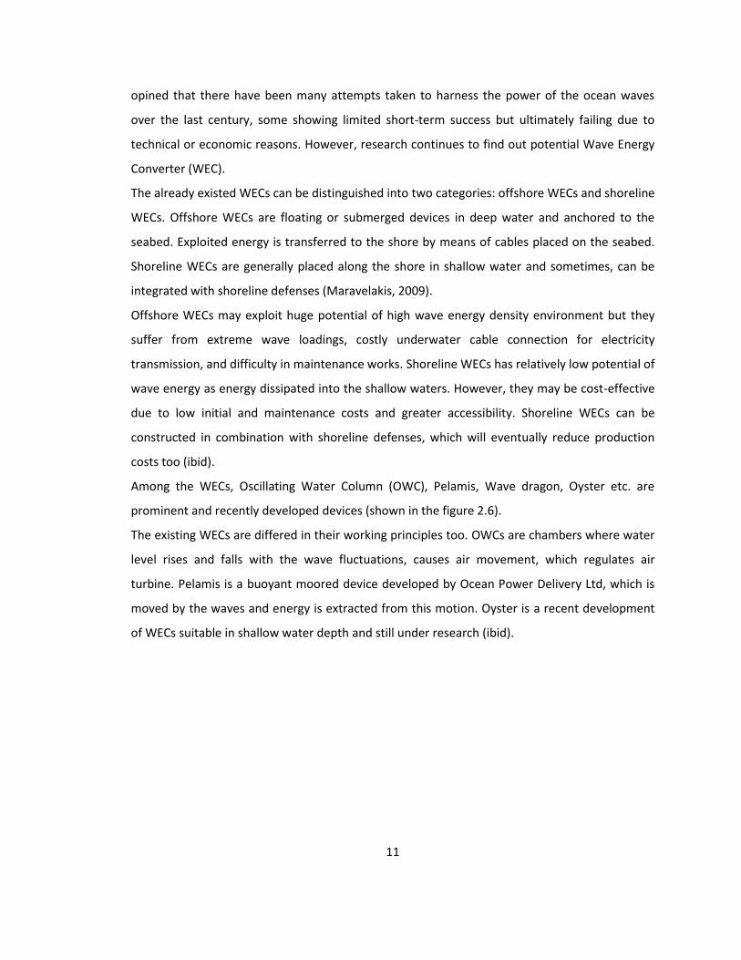
Figure 4.4-4.5 show that overtopping decreases at 150 angles of wave approach, but increases

again at 300 angles of wave approach.

Figure 4.4: Overtopping at different angles (Freeboard 1.0 meter)

Figure 4.5: Overtopping at different angles (Freeboard 1.5 meters)

42

Overtopping depend not only significant wave heights and angles of wave approach, but also on

the wave periods (Figure 4.6). Higher wave period increases overtopping. Owen (1980) includes

wave period in the prediction calculation (but seem to be over emphasized) and Van der Meer

(1995) ignores wave period in non-breaking wave overtopping prediction. This is a reason of

wide variations of performances of the overtopping prediction formulas (figure 4.2-4.3).

Figure 4.6: Wave period dependence of overtopping (Freeboard 1.5 meters) 4.4 Hydraulic performance at oblique waves

Hydraulic performances of the composite seawall at 00, 150 and 300 angles of wave approach are

given in the tables 4.10 to 4.12. Hydraulic performances are presented here for 1.0m and 1.5m

freeboards in order to look at the differences at different angles of wave approach. Maximum

hydraulic efficiencies are measured about 36.5 %, 33.6% and 28.8% at 150, 00 and 300 angle of

wave attack respectively.

43

Table 4.10: Hydraulic performance of the composite seawall for φ= 00.

Free board

(Rc) m

Time period (T) sec

Wave length (L) m


Measured mean


Wave power (Pw)

KW/m


KW/m


(Pcr/Pw)×100 in %

1.0 (d=9.0m)

7.54

63.3

0.5 0.028 2.13 0.28 13.1

0.9 0.117 6.91 1.18 17.1

1.05 0.195 9.4 1.96 20.9

5.87

45.5

0.7 0.044 3.38 0.44 13

0.95 0.085 6.23 0.85 13.6

1.2 0.202 9.95 2.03 20.2

4.26

27.4

0.85 0.058 3.31 0.58 17.5

1.2 0.161 6.6 1.62 24.5

1.65 0.345 12.48 3.47 27.8

1.5 (d=8.5m)

7.92

65.2

0.9 0.018 7.01 0.27 3.9

1.15 0.149 11.45 2.25 19.7

1.6 0.268 22.16 4.04 18.2

6.08

46.7

0.6 0 2.56 0 0

1 0.032 7.12 0.48 6.7

1.2 0.112 10.26 1.69 16.5

4.10

25.5

0.75 0.022 2.48 0.33 13.3

1.25 0.144 6.88 2.17 31.5

1.8 0.318 14.27 4.8 33.6

44

Table 4.11: Hydraulic performance of the composite seawall for φ= 150

Free board

(Rc) m

Time period (T) sec

Wave length (L) m


Measured mean


Wave power

(Pw) KW/m


KW/m


(Pcr/Pw)×100 in %

1.0 (d=9.0m)

7.76

65.6

0.8 0.025 5.56 0.25 4.5

1.25 0.127 13.57 1.28 9.4

1.65 0.24 23.65 2.41 10.2

5.92

46.1

1.25 0.032 10.9 0.32 2.9

1.5 0.116 15.7 1.17 7.5

1.75 0.224 21.36 2.25 10.5

3.91

23.8

1.3 0.057 6.95 0.57 8.2

1.9 0.283 14.84 2.85 19.2

2.5 0.475 25.7 4.78 18.6

1.5 (d=8.5m)

7.76

64.2

1.1 0.045 10.4 0.68 6.5

1.5 0.134 19.33 2.02 10.5

1.9 0.336 31.02 5.07 16.3

5.80

44

1.25 0 10.67 0 0

1.5 0.06 15.37 0.91 5.9

2 0.165 27.32 2.49 9.1

3.91

23.5

1.75 0.067 12.65 1.01 8

2.3 0.356 21.86 5.37 24.6

2.75 0.756 31.25 11.4 36.5

45

Table 4.12: Hydraulic performance of the composite seawall for φ= 300

Free board

(Rc) m

Time period (T) sec

Wave length (L) m


Measured mean


Wave power

(Pw) KW/m


KW/m


(Pcr/Pw)×100 in %

1.0 (d=9.0m)

7.74

65.6

0.85 0.114 6.28 1.15 18.3

1.15 0.216 11.49 2.18 19

1.4 0.356 17.03 3.58 21

6.02

47.2

1 0.082 7.09 0.82 11.6

1.4 0.229 13.9 2.31 16.6

1.8 0.408 23 4.1 17.8

4.0

24.6

1.4 0.16 8.26 1.61 19.5

1.95 0.356 16.03 3.58 22.3

2.4 0.516 24.28 5.19 21.4

1.5 (d=8.5m)

7.74

63.8

0.9 0.095 6.94 1.43 20.6

1.25 0.197 13.38 2.97 22.2

1.6 0.349 21.93 5.26 24

6.17

47.8

1.15 0.056 9.57 0.84 8.8

1.6 0.127 18.53 1.92 10.4

1.9 0.247 26.13 3.73 14.3

3.91

23.4

1.7 0.101 11.9 1.52 12.8

2.25 0.314 20.85 4.74 22.7

2.65 0.553 28.92 8.34 28.8

Figure 4.7-4.8 show the hydraulic power generated at the crest of the seawall at different angles

of wave approach for freeboards 1.0 m and 1.5 m. Hydraulic power increases with the increasing

wave heights in both freeboards. Hydraulic power generated decreases at 150 angle of wave

approach, but increases at 300 angle of wave approach. The data of the hydraulic power at 300

angle of wave approach are more scattering and this scattering is increased at 1.5 m freeboard

(figure 4.8).

46

Figure 4.7: Hydraulic power at different angles (Freeboard 1.0 meter)

Figure 4.8: Hydraulic power at different angles (Freeboard 1.5 meters)

47

Figures 4.9-4.10 are graphical presentations of the realized hydraulic efficiencies at various

significant wave heights of 00, 150 and 300 angles of wave attack for freeboards 1.0m and 1.5m.

These two graphs are rather more scattered, but the general trend is that hydraulic efficiency

decreases with increasing angle of wave approach.

Figure 4.9: Hydraulic efficiency at different angles (Freeboard 1.0 meter)

Figure 4.10: Hydraulic efficiency at different angles (Freeboard 1.5 meters)

48

4.5 Performance optimization with tidal variations

Tidal variations are very important for performance measurements of composite seawall of

WEC. Higher water level during high tide increases hydraulic (overtopping) performance while it

reduces effective hydraulic head, meaning that it reduces energy production. During high tide, if

water level reaches at the crest of the ramp (meaning freeboard becomes zero), overtopping is

maximum, but there is no energy production because it does not generate hydraulic head.

Similarly during low tide, increased freeboard reduces overtopping. If overtopping is sufficient to

keep the water reservoir full, then it increases energy production due to increased hydraulic

head. But after certain freeboard increased, energy production reduces due to insufficient

hydraulic head caused by insufficient overtopping. Hence it can be concluded that this type of

composite seawall for WECs is especially suitable for the places in which tidal ranges are very

low (about 1.0 m or less), compared with the significant wave heights.

An analysis of performance optimisation of the composite seawall is made against tidal

variations of 1.0 m during neap tide and 2.0 m during spring tide based on the following

conditions. Results of the analysis are shown in the table 4.13.

Considering tidal range= 2 m (during spring tide) and tidal range =1 m (during neap tide) Tidal period =12 hours 25.2 minutes =12.42 hours Flood tidal period=6.21 hours Ebb tidal period=6.21 hours Average range of the significant wave height = 0.5 m to 2.5 m Angle of wave attack generally remains normal to the structure. Considering mean water level (MWL) at 0.0 meter, this means 1.0 meter free board. Different stages of tidal variations are as follows. Freeboard = 0.0 meter during Higher High Water Level (HHWL) Freeboard = 0.5 meter during High Water Level (HWL) Freeboard = 1.0 meter during Mean Water Level (MWL) Freeboard = 1.5 meter during Low Water Level (LWL) Free board =2.0 meter during Lower Low Water Level (LLWL)

49

Table 4.13: Performance optimization against tidal variations

Wat

er

leve

l

Fre

ebo

ard

(R

c), m

Ave

rage

sig

. w

ave

hei

ght

(Hs)

, m

Rat

io,

(Hs/

Rc)

Ave

rage

mea

sure

d

ove

rto

pp

ing

rate

,

(q M

), m

3 /sec

/m

Ave

rage

Hyd

rau

lic

po

wer

at

cres

t.

(Pcr

), K

W/m

Ave

rage

Hyd

rau

lic

effi

cien

cy, i

n %

HHWL 0 - - - - -

HWL 0.5 0.76 1.52 0.216 1.11 26.6

MWL 1.0 1.0 1.0 0.109 1.38 18.6

LWL 1.5 1.1 0.73 0.097 1.78 15.9

LLWL 2.0 1.78 0.89 0.101 2.83 11.1

Average overtopping rate during neap tide= 0.128 m3/sec/m Average hydraulic power during neap tide = 1.41 KW/m Average annual power production (for given wave climate and tidal range) = 12.35 MWh/m Average hydraulic efficiency during neap tide= 19.7 % Average hydraulic performances of the composite seawall against the average ratio of the

significant wave height and freeboard (Hs/Rc) are shown in the figure 4.11. Overtopping

increases with increasing ratio, while achievable hydraulic power at crest decreases. Optimized

overtopping and hydraulic power at the crest level are found at the ratio of about 0.75.

Hydraulic efficiency increases with the increasing the ratio with a maximum of about 27%.

Figure 4.11: Hydraulic performance with Hs/Rc ratios

50

4.6 Outfall design

Reservoir of composite seawall collects water from wave overtopping and creates hydraulic

head. HPW converts this head into power and release the collected water. The released water

needs a suitable outfall to return to the sea. Main design purposes are to protect the outfall

from wave action and maximize energy production. Three types of outfalls can be considered in

these purposes.

Submarine outfall: Pipe outfall can be placed at deepwater, which will be free from wave

motion. As outfall will be free from wave action, it will provide calm water level inside the pipe

and hence it will maximize the power production (figure 2.12). Submarine outfall could be costly

to install and mouth of the outfall is subject to siltation and hence regular maintenance could be

required. Frictional losses could be involved due to pipe length. Costs of installation and

maintenance and frictional losses can be reduced by optimizing the length of the pipe and depth

of water against wave effects.

Sub-surface outfall: Passage of water will be controlled by a flushing gate at the sub-surface

outfall. This outfall will allow one way passage of water. This gate becomes open during

recession of wave (at trough) and remains close when wave hits (at crest) on the gate. The gate

is widely used to prevent saline water intrusion during high tide into agricultural field (figure

2.13). It could be very efficient and less costly for composite seawall. But, tidal cycle is about

12.5 hours whereas wave cycle is a matter of few seconds. Hence, main disadvantages could be

wear and abrasion, which requires regular maintenances like greasing of the moving parts.

Wave breaker screen: A screen of vertical pile can be installed in front of the surface outfall.

Vertical piles can be supported by armor rocks in front of it like breakwaters. There should be

gap between vertical piles and outfall for easy release of the discharge. This type of outfall will

be easy for construction and maintenance and relatively cheap. Outfall discharge will be

affected by flow of water, when wave crest hits the screen and hence energy production may be

disrupted and reduced.

51

An initial design of this type of outfall has been done in the project. Model of the designed

outfall was built and tested in the wave basin (figure 3.3). Results of the model test simulations

(converted into prototype results) are shown in the table 4.14.

Table 4.14: Realized test results of the designed outfall

Free board

(m)

Wave period, Tm,

(sec)

Sig. wave height, Hs,

(m)

Swelling of water level at the outfall, (m)

Decrease of the hydraulic

head, %

Fluctuation range of the water level at the outfall, (m)

1.0

7.71

1.0 0.025 2.5 0.15

1.25 0.05 5 0.2

5.73

2.0 0.1 10 0.3

2.5 0.125 12.5 0.35

3.96

1.5 0.05 5 0.15

2.25 0.1 10 0.3

1.5

8.0

0.75 0.025 1.7 0.15

1.25 0.05 3.3 0.2

6.01

1.5 0.125 8.3 0.3

2.25 0.175 11.7 0.35

4.03

0.5 0.05 3.3 0.2

1.25 0.1 6.7 0.3

Table 4.14 shows that the designed wave breaker screen decreases effective hydraulic head of

the composite seawall up to 12.5%. Fluctuation range of the water level at the outfall of the

composite seawall becomes up to 35 cm. Swelling of the water level at the outfall due to water

discharge and wave action reaches up to 17.5 cm above MWL. Higher wave heights create

higher swelling and water level fluctuation range.

It could be concluded based on the model test results shown in the table 4.14 that the design

wave breaker screen is effective and suitable for composite seawall WEC. Detail calculations of

the wave breaker screen design are shown in the appendix-IV. Armor rocks are designed

following rubble mound breakwater design (Hudson formula) methods (Kamphuis, 2002). A

sketch of the designed outfall layout is shown in the appendix- V.

52

4.7 Simple experimental observations

The interactions between waves and the structure have been carefully observed during the

simulation experiments. The water depth in the wave basin was neither shallow nor deep

considering wave parameters. Overtopping was green type and non-breaking and it was not

uniformly distributed over the length of the ramp, especially in case of oblique wave

approaches.

Wave-structure interactions: Wave shoaling occurs on the slope of the structure and wave

reflection on the ramp of the composite seawall creates reflected waves while overtopping over

the ramp. Reflected waves interact with the incoming waves and generate standing waves.

Properties of the standing waves (either perfect or imperfect) depend on the wave periods and

position of the composite seawall with respect to incoming waves. After 4-5 cycles of wave (as

distance between wave peddle and ramp of the seawall is about 2.0 m), the reflected waves

again reflect on the wave peddle and thus the whole wave basin becomes fully random.

Sloshing: While overtopping of the waves over the ramp and water enters into the reservoir,

sloshing of the reservoir water occurs. Relatively higher waves reflect on the vertical seawall

behind the ramp after overtopping, which generates irregular movement of the reservoir water.

This reflection causes spilling of the reservoir water back into the wave basin, especially when

reservoir is full.

Funnelling effects: Positions of the composite seawall in the wave basin are set at angles of 00,

150 and 300 with the incoming waves. Oblique positions of the composite seawall along with the

side of the wave basin look like a funnel shape. Waves converge in this funnel shape portion and

create swelling of the water surface, which increases wave height in the narrow portion of the

wave basin (figure 4.12). This funnelling effect becomes very important in overtopping and it

causes bulk overtopping at the corner of the composite seawall. Oblique wave approach

normally reduces overtopping in the real sea state, while funnelling effect increases overtopping

in the 3-D physical model. These effects become vivid at 300 angle of wave approach and are the

main cause of increasing overtopping performance and hydraulic power performance of the

composite seawall, while it should be decreasing (figure 4.4-4.5 and figure 4.7-4.8).

The funnelling effect occurs because of errors in model set up; length of the composite seawall

(1.2 m long) is very large compared to the width of the wave basin (1.5 m wide). Although the

model is set for 3-D conditions, it seems acting as 2-D model and producing funnelling effects.

53

To reflect the 3-D physical modelling of a real sea state condition, the length of the composite

seawall should be smaller than the used one. Because of that there is no barrier like sides of the

wave basin in real sea state and hence oblique waves do not create funnelling effects in the real

sea state conditions.

Figure 4.12: Funnelling effect at oblique waves of 300 4.8 Market potential of composite seawall for WECs

Ocean wave energy is an important source of renewable energy. Rapid depletion of fossil fuel

and increasing concern of environmental consequences has forced world community to develop

suitable techniques to extract renewable energy in a cost effective way. Although considerable

improvement has been made during last decades, renewable energies are not ready yet to

compete with other conventional energies.

Composite seawall for WECs can be developed as a dual purpose structure, for both sea

defenses and energy production. It cannot compete in the energy market alone with fossil fuel

due to high production costs and low conversion efficiencies (about 15-20%). However, it can be

cost effective only if it is considered as byproduct of the seawall. Composite seawall for WECs

could be suitable in such a remote place (usually Islands), where conventional energy supply

would be highly expensive and nearly impossible.

54

Chapter V

Conclusion

5.1 Conclusions

From analysis of the model simulation results, the following conclusions can be made:

Overtopping Prediction formulas (Owen (1980) and Van der Meer (1995)) are widely

varying in predictions. However, Van der Meer (1995) is found more ordered and

relatively good than Owen (1980) in predictions.

Maximum hydraulic efficiency of the composite seawall is about 37 %. Average hydraulic

efficiencies are about 26.6%, 18.6%, 15.9% and 11.1% for the freeboard of 0.5m, 1.0m,

1.5m and 2.0m respectively. Hydraulic power (generated at the crest of the ramp)

increases with increasing wave heights and decreases with increasing freeboard.

Minimum wave heights required for hydraulic power generation are about 0.4 m, 0.6 m,

0.8 m and 1.2 m for freeboard 0.5 m, 1.0 m, 1.5 m and 2.0 m respectively. Hydraulic

efficiencies at 1.0 m and 1.5 m freeboards are more ordered and consistent than that at

other freeboards for given Mediterranean Sea climatic conditions.

Both overtopping and generated hydraulic power decrease at oblique waves. Maximum

hydraulic efficiencies are measured about 33.6%, 36.5% and 28.8% at 00, 150 and 300

angle of wave attack respectively.

Average hydraulic efficiency of a composite seawall (having 1.0 m freeboard) is about

20% in case of 1.0 m tidal variation. Composite seawall for WECs is not suitable for high

tidal variations and low wave heights. Average annual power production of composite

seawall in Mediterranean Sea climatic conditions is about 12.35 MWh per meter of

seawall width.

55

Hydraulic efficiency of the composite seawall increases with increasing the ratio of wave

height and freeboard (Hs/Rc), while achievable hydraulic power at crest decreases.

Optimized overtopping and hydraulic power at the crest level are found at the ratio of

about 0.75.

Wave breaker screen (which is designed and model) is found suitable at the outfall.

However, wave breaker screen decreases hydraulic head of the composite seawall up to

12.5%.

5.2 Further study

Further study is proposed by repeating the 3-D physical model experiments with a

shorter composite seawall compared to the width of the wave basin. Shorter composite

seawall for WECs might avoid funnelling effects in the model study and might give more

reliable performance prediction for oblique wave approaches.

A composite seawall for WECs can be built as a case study based on the model study

results. Prototype study results might give actual energy production potentiality of this

type of coastal structure.

56

References

ACU-GATE, (2003), Grade water management systems: http://www.grandeinc.com/ACU-

GATE%20Page.htm, date accessed 12/05/2010

BWDB, (1988), Standard design manual, Vol.-1: Standard design criteria, Standard design

manual committee, Bangladesh Water Development Board, Office of the Chief Engineer

(Design), BWDB, Dhaka

Besley, P., (1999), Wave overtopping of seawalls: design and assessment manual, Hydraulics

Research Wallingford, R &D Technical Report, W178, ISBN 1 85705 069 X

Canning, A., (2009), Investigation into the use of composite seawalls for power generation and

energy dissipation in extreme conditions, School of Civil Engineering and the Environment,

University of Southampton

Chaplin, J., (2009), Notes on linear wave theory and wave transformations, lecture notes, School

of Civil Engineering and the Environment, University of Southampton

Dalrymple, R.A., (1985), Introduction to physical models in coastal engineering, in physical

modeling in coastal engineering, edited by Dalrymple R.A., pp.3-9

Elmosa, (1989), Seawater intake systems and sea outfalls: http://www.amecosys.com/elmosa/,

date accessed 12/05/2010

EurOtop, (2007), Wave overtopping of sea defences and related structures: assessment manual,

Environmental Agency, UK: www.overtopping-manual.com, date accessed 15/03/2010

Energy resources, (2010), Wave power: http://home.clara.net/darvill/altenerg/wave.htm, date

accessed 18/02/2010

http://www.grandeinc.com/ACU-GATE%20Page.htm

http://www.grandeinc.com/ACU-GATE%20Page.htm

http://www.amecosys.com/elmosa/

http://www.overtopping-manual.com/

http://home.clara.net/darvill/altenerg/wave.htm

57

Hughes, S.A. (1993), Physical models and laboratory techniques in coastal engineering, World

Scientific, Singapore, 1993

HR Wallingford, (2010), Wave overtopping calculation tool: http://www.overtopping-

manual.com/calculation_tool.html, date accessed 03/02/2010

Kumer, P.R.D. and Sarma, R.V., (1990), Physical oceanographic investigation procedure for a sea

outfall project, A paper presented at all India seminar on “Sea Outfalls”, September 1990

Kamphuis, J.W., (2002), Introduction to Coastal Engineering and Management, World Scientific,

Singapore

Kane, M., (2005), California small hydropower and ocean wave energy resources, staff paper

presented at California Energy Commission, Sacramento, California, May 2005.

Kofoed, J. P., (2005), Model testing of the wave energy converter Sea wave Slot-Cone Generator,

Hydraulics and Coastal Engineering No. 18, ISSN: 1603-9874, Dept. of Civil Eng., Aalborg

University, 2005

Kortenhaus, A., Van der Meer, J., Burcharth, H.F., Geeraerts, J., Pullen, T., Ingram, D., and Troch,

P., (2005), CLASH workpakage 7: Quantification of measurement errors: model and scale effects

related to wave overtopping, Leichtweib Institute for Hydraulics, Germany

Le Mehaute B., (1976), Similitude in coastal engineering, Journal of the waterways, harbors and

coastal engineering division, 102, WW3, pp.317-335

Ludwig, R.G., (1988), Environmental Impact Assessment: Siting and design of submarine outfalls,

Rio de Jenerio, 1988

Leonard energy, (2007), Energy technology: sea slot-cone generator: http://www.leonardo-

energy.org/seawave-slot-cone-generator-ssg, date accessed 22/04/2010

http://www.overtopping-manual.com/calculation_tool.html

http://www.overtopping-manual.com/calculation_tool.html

http://www.leonardo-energy.org/seawave-slot-cone-generator-ssg

http://www.leonardo-energy.org/seawave-slot-cone-generator-ssg

58

Mori, M., Yamamoto, Y. and Kimura, K., (2008), Wave force and stability of upright section of

high mound composite seawall, ICCE, Hamburg, September 2008.

Maravelakis, N., (2009), Experimental investigation of a novel composite seawall for wave

energy conversion, School of Civil Engineering and the Environment, University of Southampton,

October, 2009

Muller, G., Canning, A., Magagna, D., Stagonas, D., Warbrick, D., (2009), Composite seawalls for

wave energy conversion, School of Civil Engineering and the Environment, University of

Southampton, 2009

Muller, G., (2009), Notes on Maritime Energy and Coastal Engineering, Lecture presentations,

School of Civil Engineering and the Environment, University of Southampton, 2009

OCS, (2010), OCS Alternative Energy and Alternate Use Programmatic EIS:

http://ocsenergy.anl.gov/guide/wave/index.cfm, date accessed 03/02/2010

Pelamis wave power, (2010), http://www.pelamiswave.com/, date accessed 22/05/2010

Rise, (2008), Wave power: http://www.rise.org.au/info/Tech/wave/index.html, date accessed

18/02/2010

Svendsen, I.A., (1985), Physical modeling of water waves, in physical modeling in coastal

engineering, edited by Dalrymple R.A., pp.13-47

Soliman, A., (2003), Numerical study of irregular wave overtopping and overflow, PhD thesis,

School of Civil Engineering, University of Nottingham, November 2003

Steinhardt, J. and Hommer, B., (2006), Basics of hydro-self flushing system in rectangular tanks,

round tanks and tunnel sewers, Taunusstuin, Germany, September 2006

http://ocsenergy.anl.gov/guide/wave/index.cfm

http://www.pelamiswave.com/

http://www.rise.org.au/info/Tech/wave/index.html

59

Troch, P., Geeraerts, J., Walle, B.V., Rouck, J.D., Damme, L.V., Allsop, W., and Franco, L., (2004),

Full-scale overtopping measurements on the Zeebrugge rubble mound breakwater, Journal of

Coastal Engineering, Vol: 51 (2004) P. 609-628, June 2004

Van der Meer, J.W., (1993), Conceptual design of rubble mound breakwaters, The Netherlands

Van der Meer, J.W. and others, (2002), Technical report: wave run-up and wave overtopping at

dikes, Technical advisory committee on flood defence, Delft, May 2002

Wave dragon, (2005), Wave dragon technology: www.wavedragon.net, date accessed

24/03/2010

Wave energy, (2005), Technology: http://www.waveenergy.no/WorkingPrinciple.htm, date

accessed 22/04/2010

Wikipedia, (2010), Wave power: http://en.wikipedia.org/wiki/Wave_power, date accessed

18/02/2010

Wikipedia, (2010), Mediterranean Sea: http://en.wikipedia.org/wiki/Mediterranean_Sea and

http://en.wikipedia.org/wiki/Tidal_range, date accessed 27/05/2010

http://www.wavedragon.net/

http://www.waveenergy.no/WorkingPrinciple.htm

http://en.wikipedia.org/wiki/Wave_power

http://en.wikipedia.org/wiki/Mediterranean_Sea

60

Appendix I Sample calculations of wave analysis and overtopping Angle = 0 deg., Freeboard 10mm (0.5 m in prototype) Deep water depth= 190 mm (9.5 m in prototype) Shallow water depth= 135 mm (6.75 m in prototype) Both depths are compared with d/L ratio, and both are found transitional water depths. Significant wave height and wave period are collected from simulations results using Excel spreadsheets. Definition of significant wave height is followed in the wave analysis. Wave height and wave period are converted into full scale prototype. Wave height in model = 10 mm (Measured from Excel spreadsheet results of the model simulation) Hence, wave height in prototype = 10×50/1000 m =0.5 m (Geometric scale 1:50) Wave period in model =1.064 sec (Measured from Excel spreadsheet results of the model simulation) Hence, wave period in prototype= 1.064×7.07 sec =7.52 sec (Time scale 1:7.07) Wave length is measured by trial and error method from the following equation (table 2.1) of the transitional water depth.

Hence, Wave length (L) in prototype for T=7.52 sec and d= 9.5 meter is 64.3 m Water depth is checked by d/L ratio and it is transitional water depth. Surface area of the water reservoir in the seawall = 1200×160 mm2= 0.192 m2

Collected water in the model =0.00132 m3 (for T=1.064 sec and Hdeep= 10 mm in the model simulation) No of cycles in each simulation = 4 Simulation time = 4×1.064=4.256 sec (Model) Simulation time = 4.256×7.07 =30.09 sec (Prototype) Measured overtopping rate in the model =0.00132/ (1.064×4)/1.2= 0.000258 m3/s/m (Length of the model is 1.2 meters) Collected water in prototype (Measured mean overtopping rate) qM= 0.00132×125000/30.09=3.905 m3/sec =0.091 m3/sec/m (Volumetric scale= 1:125000, Length of the prototype = 60 m) Using equation 3.1, qM= 0.000258×501.5= 0.091 m3/s/m

61

Appendix II

Sample prediction calculations of overtopping Owen and Besley predictions Owen (1980) overtopping formula reads (Equations 3.2 and 3.3):

Which is valid only when

Slope of the structure = 1:1.75 From table 3.2, ao=0.009115, b0=20.75 (By linear interpolation) Smooth seabed, уr =1.0 When Freeboard, Rc= 0.5 m and Time period, Tm=7.52 sec, Significant wave height, Hs= 0.5 m (These values are taken from model simulations) g= 9.81 m2/sec R*=0.03, (This is within the range of 0.05 and 0.30) (equation 3.3) Putting these values in the prediction equation (3.2) Hence, predicted overtopping rate, qOwen = 0.2 m3/sec/m Van Der Meer predictions Non-breaking and green type of overtopping occurs in the model simulations (from observations). Therefore, maximum overtopping rate is calculated from the following equation (3.5):

Freeboard, Rc = 0.5 m

Significant wave height, Hm0 = 0.5 m (from model simulation) g =9.81 m2/sec Surface roughness factor, Yf=1.0 (smooth seabed) Factor for oblique wave attack, yβ=1.0 (normal wave attack) Putting these values in the equation (3.5) Predicted overtopping rate, qVDM=0.036 m3/s/m

Slope of the seawall

Values of ao

Values of bo

1:1 0.00794 20.1

1:1.5 0.00884 19.9

1:2 0.00939 21.6

1:2.5 0.0103 24.5

1:3 0.0109 28.7

1:3.5 0.0112 34.1

1:4 0.0116 41.0

62

Appendix III

Sample calculations of hydraulic performance Angle = 0 deg., Freeboard 10mm (0.5 m in prototype) Deep water depth= 190 mm (9.5 m in prototype) Wave length is measured by trial and error method from the following equation (table 2.1) of the transitional water depth.

Hence, Wave length (L) in prototype for T=7.52 sec and d= 9.5 meter is 64.3 m Hence, d/L= 9.5/64.3 =0.148, Water depth is checked by d/L ratio and it is transitional water depth. Celerity of the corresponding wave is determined by the following equation (table 2.1)

C= 8.56 m/sec Group velocity is determined by the following equation (table 2.1)

n= 0.797 Cg= 0.797×8.56 =6.83 m/sec Energy density is determined (table 2.1) by E=ρgH2/8 Sea water density ρ=1025kg/m3 Gravitational acceleration g=9.81 m2/sec Wave height H= 0.5 meter Hence, wave power Pw= ECg= Cg× ρgH2/8 =6.83×1025×9.81×0.52/8 =2146 Watt/meter of width So, Pw= 2.15 KW/m Measured mean overtopping rate, qM= 0.091 m3/sec/m. Hydraulic power related to wave height at crest, Pcr= qM Rc ρg=0.091×0.5×1025×9.81/1000=0.46 KW/m (equation 3.6) Therefore, Hydraulic efficiency of the seawall= 0.46/2.15 ×100= 21.4%

63

Appendix-IV

Sample calculations of outfall design: Wave breaker screen

Considering design wave height = 3.0m

And considering design storm wave height= 4.0m (for armor rock design only)

Height of the vertical piles= 3.0m above MWL

Length of the vertical pile screen = 5.0m

Diameter of pile = 0.4m

Gap between two piles= 0.2m

No of piles required = 8

Width of the outfall mouth= 1.0m, centrally position behind the pile screen

Height of the outfall mouth = 1.0m above MWL

Gap between pile screen and outfall mouth= 1.0m

Primary armor layer: Two layers of rock armor on the slope in front of the vertical pile screen

Slope of the armor layer=1:2

Density of seawater =1025 kg/m3

Density of the rock= 2650 kg/m3

Damage co-efficient for quarry rock= 4.0

Mass of the primary armor rock (following Hudson formula):

Ma= 5320 kg= 5 tons

Diameter of the primary rock armor= 0.8m

Thickness of the primary rock armor layer=1.6m

Primary armor rock will be placed up to 3.0m below LLWL

Width of the armor layers= 5.0m

Filter layer: Two layers of rock beneath the primary armor layers

Mass of filter rock (Ma/10) = 0.5 tons

Diameter of the filter rock = 0.1m

Thickness of the filter rock layer=0.2m

64

Appendix V

Sketch of the designed outfall: Wave breaker screen A

Composite seawall for WEC HPW Seawall CCo weir/gate Ramp Wave overtopping Piles and armor rocks A Plan and top view of the outfall Pile (round) arrangement (Pile dia @0.4m and gap 0.2m)

3.0 m above MWL

Primary armor

3.0 m 1.0m

5.0 m MWL

LLWL 1.0m weir/ gate

Filter layer

1:2

Cross-section of the outfall (Section A-A)

c marine engineering and management comem

Documents