x.

NASA Contractor Report 189652, Volume I

/i_- c _.I--

//'7,-/7(..

An Installed Nacelle Design Code Using aMultiblock Euler Solver

Volume I: Theory Document

H. C. Chen

-=

\\

N

Boeing Commercial Airplane Group

Seattle, Washington

Contract NAS1-18703

September 1992

[U/Lq/ National Aeronautics andSpace Administration

Langley Research CenterHampton, Virginia 23665-5225

,.o

N

N U ,,..,@, t.-

Z,._ Li,JG_3E

|

•-J _. 0t.u O 0 ¢J

Z_ =6 C

;P' wF,.- p,-

,._ 0.._,.J C l.,,-4 _ C) ,,,..,=,I wu_ ,,_

.-.. ¢3

_. u./uJ Z t_I ..I =jt_,.,,

_J -J _ =C U

O 0I _3 .J).- _._

ZZ -¢_0-

o

https://ntrs.nasa.gov/search.jsp?R=19920022982 2020-04-06T06:43:13+00:00Z

TABLE OF CONTENTS

1.0 Summary .................................................... 1

2.0 Introduction .................................................. 2

3.0 Methodology ................................................. 4

3.1 Theory ................................................... 4

3.2 Implementation ............................................ 7

3.3 Findings ................................................. 10

3.3.1 Geometry Closure ...................................... 10

3.3.2 Surface Smoothing ..................................... 10

4.0 Results and Discussions of Test Cases ............................. 13

4.1 Isolated Nacelle Design ..................................... 13

4.2 Installed Nacelle Design ..................................... 15

5.0 Conclusions ................................................. 19

6.0 Acknowledgement ........................................... 20

6.0 References .................................................. 21

A

Appendix ................................................... 23

Reduction of Rotation ........................................ 24

B Data Smoothing .............................................. 26

B.1 Least-Squares Smoothing ................................... .26

B.2 Smoothing by Averaging .................................... 27

B.3 Asymptotic Behavior ....................................... 29

PRECEDING PAGE BLA_K I',]GT F!LMEDiii

n

1.0 Summary

An efficient multiblock Euler design code was developed for designing a

nacelle installed on geometrically complex airplane configurations. This approach

employed a design driver based on a direct iterative surface curvature method

developed at NASA-Langley. A general multiblock Euler flow solver was used for

computing flow around complex geometries. The flow solver used a finite-volume

formulation with explicit time-stepping to solve the Euler equations. It used a

multiblock version of the multigrid method to accelerate the convergence of the

calculations. The design driver successively updated the surface geometry to

reduce the difference between the computed and target pressure distributions. In

the flow solver, the change in surface geometry was simulated by applying surface

transpiration boundary conditions to avoid repeated grid generation during design

iterations. Smoothness of the designed surface was ensured by ahemate

application of streamwise and circumferential smoothings. The capability and

efficiency of the code was demonstrated through the design of both an isolatednacelle and an installed nacelle at various flow conditions. Information on the

execution of the computer program is provided in Volume II which is titled "An

Installed Nacelle Design Code Using a Multiblock Euler Solver, Vol. II: UserGuide".

2.0 Introduction

It has been roughly 40 years since the first jet transport flew. Different models

have been built by various manufacturers, and, although each manufacturer has

their own design and manufacturing approach, there are areas of common concern.

One such area is the engine installation. Historically, the aerodynamic design of

the engine nacelles and struts were done without considering the interactions

between the wing and the strut/nacelle. Some modem designs have the

nacelle/strut pitched and/or toed to line up the inlet with the local flow. Still, the

common practice is to design the wing without the nacelle/strut and to design the

nacelle as an isolated object. The designers who integrated the propulsion system

into the airframe had very little say in modifying either the wing geometry or the

nacelle geometry in order to avoid significant performance degradation from

interference between the wing and the nacelle/strut.

NASA-Langley launched an effort to look into the nacelle installation effect.

Both computational work and wind tunnel tests were carded out to gain insight on

the interference between the wing and the nacelle/strut (Ref. 1). This report

documents the development of a CFD code that would allow the designer to

reshape a nacelle installed on a wing/body/strut/nacelle configuration.

There are two major challenges in the detailed aerodynamic design of an

installed nacelle. Firstly, it requires a CFD code capable of dealing with an

extremely complex geometry as well as proper representation of the physics.

Secondly, design of the nacelle surface must be performed under the rigid

constraint of fixed leading and trailing edges.

In the beginning of the present study, we acquired NASA-Langley's direct

iterative surface curvature (DISC) design driver (Ref. 2) and the general

multiblock Euler (GMBE) solver (Refs. 3, 4, 5) as the technology basis. The

design driver provides a means for successive updates of the nacelle surface

geometry. The GMBE solver provides a flow solution for complex geometry with

proper representation of the physics except for viscous effects. In GMBE, the

capability to accept surface transpiration boundary conditions has been developed

2

to simulate the effect of surface change during design iterations. Re-gridding, to

verify the accuracy of representing surface change using the transpiration

boundary condition, is only done once for the final analysis.

The second challenge in designing an installed nacelle is related to the problem

of geometric closure. The original DISC design driver relates the geometry

change to the difference between the computed and the target pressure

distributions for each streamwise strip on the nacelle. The design driver first re-

defines a new strip in an unconstrained manner. The problem of geometry closure

at the point farthest downstream (i. e., usually the trailing edge) of a design

segment is resolved by rotating the segment hinged at a point farthest upstream (i.

e., usually the leading edge) of the segment.

In the present study, it was found that, for some test cases, the amount of

rotation required could become large during the initial design iterations. This

could affect the convergence of the iterative process. For this reason, a procedure

was developed to reduce the required rotation. The relationship between geometry

change and the difference in pressure distributions was modified before surface

redefinition. Numerical issues in implementing such a procedure have beenaddressed.

Surface smoothness is a critical requirement in the design of a three

dimensional aerodynamic surface, such as that of an installed nacelle. In the

present study, surface smoothness was ensured by applying streamwise and

circumferential smoothings for each design iteration.

There were two test cases in the study. For both test cases, design iterations

followed pre-design analyses. The first case was a two-block isolated nacelle

design problem. The design code was able to recover the target nacelle from the

corresponding target pressure at a supercritical flow condition. The second case

designed an installed nacelle on a generic twin-engined, NASA low-wing transport

configuration (Ref. 6). Results from the two test cases demonstrated the accuracy

and efficiency of the design code. The cost for a design was comparable to that of

the pre-design analysis. A user manual for the installed nacelle design code is

given in Vol. II of the present report (Ref. 7).

3.0 Methodology

The direct iterative surface curvature (DISC) method developed by Smith and

Campbell (Ref. 2) was adapted to design the external fan cowl of an installed

nacelle. The basic theory has been described previously (Ref. 2). Salient points of

the theory are discussed here. Its implementation and new findings are then

presented.

3.1 Theory

The algorithm developed by Smith and Campbell begins with the inviscid

momentum equation. For 2-D flows, the equation can be written in the streamline

curvature form,

dq/q = -_:(n)dn (1)

where q is the local speed, _: is the streamline curvature, and n is the distance

normal to the streamlines. Following the analysis of Barger and Brooks (Ref. 8),

the streamline curvature decays exponentially with respect to the distance normal

to the airfoil surface,

_:(n) = _e --cn (2)

where C is a positive constant and the subscript 0 denotes the value on the airfoil

surface. Substituting this expression into the momentum equation and integrating

gives

_o = C ln(qo/q**) (3)

where the subscript o. indicates the freestream value. If the change in speed Aqo is

small, the Taylor series expansion of w.o about qo can be performed and higher

order terms of Aq0 can be dropped. The result is

A_ = C Aqo/qo (4)

4

Letting C be proportional to r 0, as suggested in Reference 8, leads to

A_: = A1 r,Aq/q (5)

where A1 is a constant, and subscripts 0 have been dropped for simplicity. If the

perturbations caused by the airfoil are assumed to be small, it follows that: (a) the

denominator q can be expressed as q**,_) the numerator Aq can be expressed as

Au, where u is the perturbation velocity in the freestream direction, and (c) the

pressure coefficient Cp can be expressed as -2u/q**. Equation (5) then becomes

A_¢= Ar,.ACp (6)

where A=-A1/2 and ,,XOp is the change in the pressure coefficient. As the

curvature r approaches zero, a small change in curvature would result in a very

large change in the pressure coefficient Cp. This situation, however, does not

actually occur in real flows. It is the result of the assumption of Equation (2) used

in integrating the momentum equation. To circumvent this singular behavior,

Equation (6) is modified to read

A1¢= A(1 + k2)BACp (7)

where B is a constant ranging from 0.0 to 0.5 and constant A has different signs

depending on whether we are on the upper surface or on the lower surface. The

term (1 + _)B approaches unity for small values of curvature _¢. It will approach

_B for large values of curvature _¢and the resulting _B will be large for B = 0.5.

Consequently, a small change in Cp may lead to a large change in curvature. High

curvature regions usually occur at the leading edge of an airfoil or nacelle section.

In such regions, if the flow is supercritical, the large change in curvature may

affect the stability of the design iterations. Using a low value for the constant B

can stablize the iterative procedure.

The final assumption is that the change in curvature results in only small

changes in the local slope so that the relationship between the curvature and the

second derivative can be written as

5

Ay" = AK:(1 + y,2)1.5 (8)

Integrating the above equation twice will yield Ay. Equations (7) and (8) provide

the relationship between the change in surface pressure coefficient Cp and the local

second derivative y" in a locally subsonic flow. This relationship seems to work

for both subsonic and transonic flow cases, although the theory applies only to

locally subsonic flow. However, the convergence was found to be rather slow for

flows with local Mach number greater than 1.15. As discussed in Reference 9, the

relationship between the surface pressure coefficient Cp and the surface geometry

changes character as the flow becomes locally supersonic. The development of a

hybrid algorithm, similar in concept to that in Reference 9, was therefore based on

supersonic thin airfoil theory. Surface pressure coefficient Cp in a supersonic

inviscid flow is related to the local slope y' by

Cp = 2y' / [(M**) 2 - 1] v2 = C1 y' (9)

This equation can be rearranged to yield

Ay' = CACp

Differentiating with respect to x gives

(lO)

Ay" = C d(ACp)/dx (II)

Strictly speaking, the above theory is only valid for supersonic freestream Mach

numbers. Therefore, for transonic flows, the valu_fQr the "constant" C is IEft to be

determined empirically. If the freestream Mach number in Equation (9) is

replaced with a so-called "switching" (Ref. 2) Mach number of 1.15, the value of C

would be 0128. A switching Mach number is defined as a cut-off number such that

whenever the local Mach number exceeds the cut-off value, then Equation (11)

instead of Equation (8) is employed. Our experience showed that good results can

be obtained byus_ga value 0f0,16 for the constant C which under-relaxes the

changes in geometry and therefore stabilizes the process of successive iteration.

The corresponding switching Mach number is 1.05. This leads to a "hybrid"

algorithm.

6

3.2 Implementation

The algorithm presented in Section 3.1 was initially developed for the study of

2-D airfoils. It has also been applied to wings (Ref. 10) and isolated nacelles (Ref.

11). Ideally, this method should use constant azimuthal cuts of the nacelle. In

actual practice, however, not all grid lines follow the constant azimuthal cuts, due

to the presence of the strut. In this report, the method is applied to streamwise grid

lines of an installed nacelle to redesign the nacelle.

As is the case for the study of wings and isolated nacelles, the analysis of a

baseline configuration (pre-design analysis) needs to be performed. The analysis

identifies the areas requiring redesign because of undesirable flow features. Strong

shocks and severe pressure recoveries, that might cause boundary layer separation,

are a few examples of such features. Desired pressure distributions, also referred

to as target pressure distributions, are then input to the code. The term ACp is

defined as the difference between the target pressure distribution and the pressure

distribution from the pre-design analysis. The code uses equations (8) and (11) to

convert ACp into changes in second derivatives of a streamwise strip of the local

surface geometry. Integrating the changes in the second derivative in the

streamwise direction yields the new geometry. The new geometry is then re-

analyzed and the difference between the resulting surface pressure and the target

pressure is used to compute the successive changes in surface geometry second

derivatives. The process repeats until the number of geometry updates reaches a

user-specified number. The evolution of the nacelle surface Cp distributions and

geometries are stored during this process. The Cp distributions and geometries are

then displayed and compared between successive design iterations to check for

convergence. If the design iteration is insufficient to achieve convergence, then a

continuation run is made to further the design iterations. In the case where the

target Cp distribution is unrealistic, the computed Cp distributions may settle downat a level that is different from the target rather than "converge" to the target

distribution.

The geometry updates change the surface grid locations. Ideally, a new field

grid should be generated, but since grid generation is independent of both the flow

7

solver and the geometry change module, re-gridding during the iterative processcan be a tedious task. Instead, a surface transpiration model, similar to the one

used in the boundary layer displacement thickness simulation ('Ref. 12), is used tosimulate the change in surface geometry. A simple flux balance (Fig. 1) shows

that the surface transpiration velocity qn is related to the surface geometry change

by

qn = 2 [(Aypu)2 - (Aypu)l ] ] [(pl+P2) 112] (12)

where Ay = Ynew - Yold , P is the density, u is the velocity component in the x

direction, and 112 is the arc length on the old surface between stations 1 and 2.

Another option is to use the transpiration mass flux obtained from a similar

equation

(Pq)n = [(Aypu)2 - (Aypu)l] /112 (13)

The surface transpiration velocity has been used to simulate the geometry

changes for all design iterations except the final converged solution in which the

volume grid around the perturbed geometry is regenerated using a grid

perturbation method. The original volume gird is perturbed such that the surface

change introduced by Equations (8) and (11) propagates into the flow field. The

newly designed surface grid is on one face of the block, while the geometry on the

opposite face remains fixed. A blending function is used between the faces to

allow the change in surface grid to decay smoothly to zero on the opposite face.

Finally, an analysis on the new grid verifies the accuracy of representing the

geometry changes using the transpiration boundary condition.

There are two basic requirements for the grid perturbation method to work.

The first one is that the surface change does not alter the layout of the field blocks.

The second one is that the external space is divisible into two regions (Fig. 2a)

such that only the grids within a few blocks in one of the regions requires

redistribution. In addition, the surface change should be moderate in magnitude

and the first few layers of grid cells near the surface should have sufficient spacing

to prevent grid line cross-over.

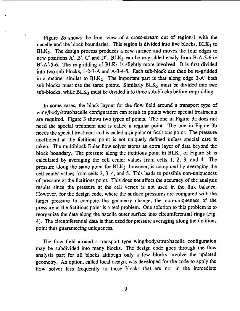
Figure 2b shows the front view of a cross-stream cut of region-1 with the

nacelle and the block boundaries. This region is divided into five blocks, BLK1 to

BLKs. The design process produces a new surface and moves the four edges to

new positions A', B', C" and D'. BLK2 can be re-gridded easily from B-A-S-6 to

B'-A'-5-6. The re-gridding of BLK1 is slightly more involved. It is first divided

into two sub-blocks, 1-2-3-A and A-3-4-5. Each sub-block can then be re-gridded

in a manner similar to BLK2. The important part is that along edge 3-A' both

sub-blocks must use the same points. Similarly BLK5 must be divided into two

sub-blocks, while BLK3 must be divided into three sub-blocks before re-gridding.

In some cases, the block layout for the flow field around a transport type of

wing/body/strut/nacelle configuration can result in points where special treatments

are required. Figure 3 shows two types of points. The one in Figure 3a does not

need the special treatment and is called a regular point. The one in Figure 3b

needs the special treatment and is called a singular or fictitious point. The pressure

coefficient at the fictitious point is not uniquely defined unless special care is

taken. The multiblock Euler flow solver stores an extra layer of data beyond the

block boundary. The pressure along the fictitious point in BLK1 of Figure 3b is

calculated by averaging the cell center values from ceils 1, 2, 3, and 4. The

pressure along the same point for BLK2, however, is computed by averaging the

ceil center values from ceils 2, 3, 4, and 5. This leads to possible non-uniqueness

of pressure at the fictitious point. This does not affect the accuracy of the analysis

results since the pressure at the cell vertex is not used in the flux balance.

However, for the design code, where the surface pressures are compared with the

target pressure to compute the geometry change, the non-uniqueness of the

pressure at the fictitious point is a real problem. One solution to this problem is to

reorganize the data along the nacelle outer surface into circumferential rings (Fig.

4). The circumferential data is then used for pressure averaging along the fictitious

point thus guaranteeing uniqueness.

The flow field around a transport type wing/body/strut/nacelle configuration

may be subdivided into many blocks. The design code goes through the flow

analysis part for all blocks although only a few blocks involve the updated

geometry. An option, called local design, was developed for the code to apply the

flow solver less frequently to those blocks that are not in the immediate

9

neighborhood of geometry changes. The code will, therefore, spend relativelymore time in an area where the flow parameters are most likely to be affected bythe geometry change. This procedure should improve the efficiency of the code.

3.3 Findings

The basic geometry alteration algorithm DISC was supplied by NASA-Langley.

Problems occurred during adaptations of DISC for design code development and

study of the problems resulted in several findings. These findings were mostly

related to geometry issues such as the closure of the newly designed section, the

stability of the design iterations, and the surface smoothness. They are presented

below.

3.3.1 Geometry Closure

Most likely, the new geometry obtained by integrating Equation (8) or (11)

would not match the original surface at the downstream end of the design region

because there are no closure conditions imposed in specifying the target pressure

distribution. The original work by Smith and Campbell (Ref. 2) rotates the entire

newly designed 'segment' about the upstream end of the design region to force the

closure. A 'segment' is the new geometry from the starting location to the end of

the design region (e. g., trailing edge point). This type of rigid body rotation about

the upstream end of the design region (e. g., leading edge point) is simple and

straight forward. It works well if the amount of rotation needed to close the

section is small and monotonically decreases during design iterations. For some

test cases, however, the amount of rotation required may become large during the

early stage of design iteration. In such instances, discontinuities in slope and

curvature are introduced at the center of rotation. This may affect the convergence

of the iterative process. A procedure to reduce the amount of rigid body rotation in

the geometry closure is given in Appendix A.

3.3.2 Surface Smoothing

The new section designed by integrating Equations (8) and (11) may or may not

be aerodynamically smooth. Smith and Campbell use a 7-point least-squares curve

10

fit to smooth the section in the streamwise direction. For 3-D applications

smoothing is also needed in the circumferential direction in the case of installed

nacelles.

The least-squares curve fit uses a third order polynomial which has two forms,

depending on whether the point being smoothed is close to the leading edge or not.

Away from the leading edge the polynomial takes the form of

y = c 1 + c 2 x + c 3 x 2 + c 4 x 3 (14)

For the first 20% of the airfoil chord an additional square root term is added, thus

y = C1 + C2 X + C3 x 2 + C4 X3 + C5 X0"5 (15)

This square root term gives infinity slope at the leading edge x=0. A detailed study

of the smoothing procedure based on Equation (14), is given in Appendix B.1.

Installed nacelles designed by the current technique and smoothed by Equations

(14) and (15) should have smooth streamwise sections. However, the

circumferential grid lines may not be smooth because each streamwise section is

designed independently. In addition, the streamwise smoothing using Equations

(14) and (15) could also generate some circumferential noise in the geometry.

This situation is corrected by applying streamwise and circumferential smoothings

alternately.

The circumferential smoothing is applied to the change in geometry, Ar = rncw -

rold, where r is the radial coordinate, rather than the geometry itself. Two

smoothing techniques are available to the user. One is the 7-point least-squares

technique mentioned above. The other is a method based on averaging the

difference Ar of neighboring points. The smoothed Ar is added to rold to generate

a smooth rnew provided that the starting rold is smooth. Both techniques can

smooth out Ar in a few passes. However, smoothing by averaging is significantly

faster and has been used in this study. More details can be found in Appendix B.2.

Figure 5 plots the Ar as a function of 0 before circumferential smoothing.

11

Typically, Ar has peaks and valleys. They represent the points of maximum

geometry change. It is desirable to smooth out the peaks and valleys without

moving them to a different 0 location.

Figure 5 also shows the Ar after the smoothing step. This step consisted of

three passes of smoothing using the averaging technique. Each pass consisted of

one circumferential smoothing and one streamwise smoothing. The peaks and the

valleys have been smoothed but their 0 locations have not changed.

12

4.0 Results and Discussions of Test Cases

Two sample cases were constructed to test the design code. The first case wasan isolated nacelle and the second was an installed nacelle.

The isolated nacelle study was a good check of the DISC implementation in

GMBE. Also, experience gained from it was very helpful in the subsequent study

of the installed nacelle. From an application stand-point, the design of a suitable

isolated nacelle is the starting point for an installed nacelle design. The isolated

nacelle design used the calculated surface Cp distribution of another nacelle as the

target to check out the design process.

Study of the installed nacelle was divided into two parts. Part one was similar

to the isolated nacelle case except that the known geometry to be recovered was an

installed nacelle. Part two used a target Cp distribution that was derived by hand-

tailoring the results of a pre-design analysis. In all such design exercises, there are

of course no guarantees that a physically meaningful geometry actually exists.

4.1 Isolated Nacelle Design

An axisymmetric isolated nacelle, nacelle-1, was analyzed using the multiblock

Euler code to provide the pre-design information. A vertical symmetry plane wasused and half of the nacelle and external flow field was solved. The flow field was

covered by two blocks of grids (Fig. 6). One block covered the internal flow and

the other covered the external flow. The grid size for the intemal block was 97 x

13 x 9 in the streamwise, radial and circumferential directions respectively. The

grid size for the external block was 97 x 25 x 9. There were 49 points in thestreamwise direction on the fan cowl.

This nacelle was analyzed at M** = 0.85 and a = 0.0 degrees for 500 multigrid

steps. The converged surface Cp distribution, which is presented in the Figure 7,

indicates a strong shock. The same figure also presents the convergence history of

the surface Cp distributions. The main features of the flow, such as the pressure

peak and shock wave, were well established at 300 multigrid steps. Comparison of

Cp at 300 steps and 500 steps shows that there is only a small difference in Cp

13

distribution near the foot of the shock.

For the purpose of target Cp generation, a computational grid for a slightly

different nacelle, nacelle-2, was generated. The block layout and grid size for each

block were the same as that of nacelle-1. The x-coordinates of the grid points onthe nacelle surface are also the same between the two nacelles. The DISC method

alters the radial coordinate r at each grid point in the design region but leaves the

x-coordinate unchanged. Using the same x-coordinates for the nacelle surface grid

points ensured that the flow features contained in the target Cp could be properly

resolved as the geometry approached the target geometry of nacelle-2. Nacelle-2

was analyzed at the same flow condition as nacelle-1 for 500 multigrid steps. The

computed Cp had to be well converged to ensure that the resulting Cp (i. e., the one

to be used as the target Cp) corresponded to nacelle-2. Results, illustrated in

Figure 8, show that nacelle-2 produced a weaker shock than that of nacelle-1. The

comparison of nacelle geometries is also shown.

Nacelle-1 was then used as the initial geometry for the design with the surface

Cp from nacelle-2 as the target Cp. The entire external surface was included in the

design region. The pre-design results at 500 steps, given in Figure 7, were used to

provide the initial Cp to start the design iterations. The initial Cp had to bereasonably converged to capture the basic features of the flow, such as the pressure

peak and shock. The initial Cp, however, is not required to be fully converged and

the pre-design solutions at 300 steps could have been used to start the design.

Within each design cycle, there were 50 multigrid steps to solve the flow so as to

provide a new Cp for the updated geometry. After six cycles of design iterations,

there was good agreement between the designed surface Cp distribution and that of

the target as shown in Figure 9. The same figure also presents the geometry

recovery of nacelle-2. The convergence history of the Cp distributions, illustrated

in Figure 10, shows that the computed Cp essentially reached that of the target Cp

in the fourth cycle of the design iterations. The last two cycles improved the minor

differences in Cp distributions near the the foot of the shock. Figure 10 also

presents the convergence history of the nacelle surface geometries.

Successful completion of this isolated test case was crucial as it provided

general guidelines for the_design of the installed nacelle. This information

14

included typical numbers for multigrid steps required to establish the main featuresof the flow, the number of design cycles required for convergence to the final

design, and the number of multigrid steps required for each geometry update. Thecost of a design, as measured by the total number of multigrid steps required after

the pre-design analysis, was comparable to that of the pre-design analysis. Thepre-design analysis took nine minutes of CPU time on a Cray Y-MP using one

CPU while the design iterations took six minutes. This kind of high efficiency isvital if a design code is to be used to solve large and complex problems such as theinstalled nacelle design. Efficient design codes reduce computer resource

requirements and allow for better turn'around time, a crucial element in the design

process.

4.2 Installed Nacelle Design

The baseline geometry employed in this study was the NASA-Langley 1/17

scale low-wing transport model, a wing/body/strut/nacelle configuration tested inthe 16-ft transonic tunnel. Detailed information about the model can be found in

Ref. 6. The surface grid is shown in Figure 11; the entire flow field was divided

into 32 blocks with 1,170,000 grid points. On the external surface of the fan cowl,

there are 45 points in the streamwise direction and 46 points in the circumferential

direction. Study of the installed nacelle design was divided into two parts as

mentioned previously. Part one focused on the recovery of a target Cp generated

from known geometry. Part two studied the actual design of the installed nacelle

based on a user prepared target Cp. An identical block layout and grid size was

employed in both parts of the study.

In part one, the target geometry was obtained by perturbing the external surface

geometry of the baseline nacelle and the perturbed configuration was analyzed at

M** = 0.77 and o_- 0.5 degree for 500 multigrid steps, to produce a target Cp. The

baseline geometry was used as the initial geometry to redesign the external fan

cowl. Pre-design analysis of the baseline geometry was conducted at the same

flow conditions for 500 multigrid steps as well. There were 50 multigrid steps

between design iterations to provide the Cp for the geometry updates.

In Figure 12, the initial Cp (i. e., from baseline geometry), the target Cp (i. e.,

15

from perturbed geometry), and the designed Cp distributions are plotted at four

circumferential cuts on the nacelle surface. The designed Cp (6th design cycle)

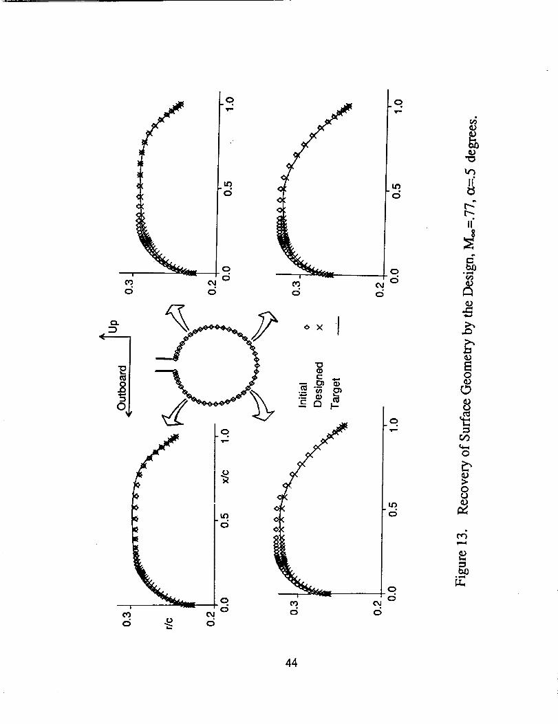
compared very well with the target Cp. Figure 13 compares the initial, target, and

designed geometries at the same circumferential locations. Chordwise

distributions of r are used to represent the surface geometry, where r is the radial

coordinate taking the nacelle centefline as the axis. Recovery of nacelle surface

geometry is shown in Figure 13. This part of the installed nacelle study establishes

confidence in the design code before it is used in part two; a realistic design case

where the final geometry is not known apriori.

In part two, the target Cp was user prepared. The specification of the target

pressure distribution depends on the intent of the design. In general, strong shocks

are to be avoided. Therefore, for a configuration whose pre-design analysis shows

strong shocks, such as nacelle-1 in the isolated nacelle study, the target pressure

distribution is relatively easy to specify. For configurations where the problems

are subtle, the guidelines for target Cp preparation are not always obvious.

The baseline geometry was again used as the starting geometry. The same pre-

design analysis used in part one was used here as well. The target Cp was obtained

by hand-tailoring the pre-design analysis results. The guiding principle was to

reduce the pressure peak that follows the leading edge expansion. This can be

seen by comparing the initial and target Cp at thefour circumferential cuts in

Figure I4. There is a potential problem with this target Cp. Note that while the

target Cp distribution has a reduced leading edge pressure peak, the detailed Cp

distribution near the leading edge, where expansion takes place, is identical to the

initial. Generally, it is difficult to alter the leading edge pressure peak without

modifying the leading edge expansion. The actual geometry required for this

target Cp most likely does not exist. Therefore, this is an extreme test case for the

design code in the sense that some compromise must be made, by the code,

between the conflicting requirements of reducing the pressure peak and

maintaining the leading edge expansion.

Interestingly, an understanding of the user's perception on how the design code

is to be used, can provide important direction and guidance for the development of

the design code. Ordinarily the design code is used to establish a fast design

16

process. Turn around time is likely to be a critical issue and target Cp would

probably be prepared rapidly. The user might be interested in modifying the pre-

design analysis results to obtain desirable features of the flow, without having to

worry about the conflicting requirements contained in the target Cp. Some users

might overlook the fact that there was a conflict in the target Cp. Others might

know exactly what they were doing but expect the design code to work out the

problems. An example of one such target Cp was illustrated in Figure 14. For

this type of target Cp, attempts to apply a geometry closure procedure, that would

maintain the leading edge geometry (e. g., using the procedure discussed in sub-

section 3.3.1), would leave very little room to modify the pressure peak. The

outcome of the design would most likely be unsatisfactory.

The designed Cp is compared with the target Cp in Figure 14. The pressure

peak was generally reduced. The leading edge expansion was different than the

target value. This appears to be the compromise required to reduce the pressure

peak. The target Cp distribution allowed no pressure change near the leading edge.This implied no geometry change would occur in this region, based on Equations

(8) and (11), without using rigid body rotation for geometry closure. Rigid body

rotation, therefore, was the source for leading edge geometry alteration and Cp

change.

Since the designed Cp was unable to reach the target Cp, the evolution of the

computed Cp was examined (see Figure 15) along a circumferential cut on the

inboard side of the nacelle. The computed Co settled down in the 6th cycle ofdesign iteration. The evolution of nacelle surface geometry r against design

iterations is also shown in Figure 15. Here, the geometry also settled down in the

6th cycle. It would be interesting to determine why the iterative process settled

down while ACp was still large, since nonzero ACp should be followed by

geometry change based on Equations (8) and (11). The reason might be that such

a geometry change is essentially cancelled by the subsequent rigid body rotation

for geometry closure. This "limit cycle" process would then allow design

iterations to settle down even for the unrealistic target Cp in the present study. The

smoothing has very little effect on this limit cycle process.

A new computational grid, based on the designed geometry, was generated for a

17

final analysis. This verification step had to be performed since the design

iterations were unable to fully achieve the target Cp. Figure 16 presents a

comparison of the designed Cp and the computed Cp based on the new grid alongthe four circumferential cuts. The excellent agreement between the two results

verifies the accuracy of representing the surface geometry change by using

transpiration boundary conditions.

The cost for the installed nacelle design was comparable to that of the pre-

design analysis. Running on Cray Y-MP using one CPU, the pre-design analysis

consumed 3 hours and 40 minutes of CPU time while the design part took 2 hours

and 20 minutes. Since the pay-off of CFD research and development relates

directly to the amount of user applications, the value of a design code is greatly

enhanced by having high efficiency. User acceptance of the design code is likely

when the cost for the design is comparable to that of the analysis.

18

5.0 Concluding Remarks

A multiblock Euler design code was developed for installed nacelle design

employing a design driver provided by NASA Langley. The effect of surface

geometry change was simulated by imposing surface transpiration boundary

conditions. Re-gridding on the converged design was used for final analysis to

verify the accuracy of such simulation. Issues, regarding the design of an installed

nacelle under the rigid constraint of fixed leading and trailing edges, were

addressed. The capability and efficiency of the design code were demonstrated by

designing isolated and installed nacelles. The code was effective in re-designing a

nacelle to weaken or eliminate a strong shock, as well as to reduce the leading

edge pressure peak. For both test cases, the cost for design was comparable to that

of the pre-design analysis. Information regarding the use of this design code isavailable in Vol. II.

19

6.0 Acknowledgement

Mainframe computing has been provided by the Numerical Aerodynamic

Simulation Complex at NASA Ames Research Center.

20

7.0 References

1. Naik, D. A., Chen, H. C., Su, T. Y., and Kao, T. J., "Euler Analysis

of Turbofan/Superfan Integration for a Transport Aircraft," AGARD Huid

Dynamic Panel Symposium on Engine-Airframe Integration, Fort Worth, TX,

October, 1991.

2. Smith, L. A. and Campbell, R. L., "A Method for the Design of Transonic

flexible Wings," NASA Technical Paper 3045, December, 1990.

3. Chen, H. C., Su, T. Y., and Kao, T. J., "A General Multiblock Euler Code

for Propulsion Integration, Volume I: Theory Document," NASA CR-187484,

Volume I, May 1991.

4. Su, T. Y., Appleby, R. A., and Chen, H. C., "A General Multiblock Euler

Code for Propulsion Integration, Volume II: User Guide for BCON,

Pre-Processor for Grid Generation and GMBE, "NASA CR-187484,

Volume II, May 1991.

5. Chen, H. C., "A General Multiblock Euler Code for Propulsion Integration,

Volume ]I1: User Guide for the Euler Code," NASA CR-187484, Volume III,

May 199 I.

6. Pendergraft, Jr., O. C., Ingraldi, A. M., Re, R. J., and Kariya, T. T.,

"Nacelle/Pylon Interference Study on a 1/17-Scale, Twin-Engine, Low-Wing

Transport Model," AIAA 89-2480, July 1989.

7. Chen, H. C., "An Installed Nacelle Design Code using a Multiblock Euler

Solver, Volume II: User Guide," NASA CR-189652, Volume II, 1992.

8. Barger, R. L., and Brooks, C. W., Jr., "A Streamline Curvature Method for

Design of Supercritical and Subcritical Airfoils," NASA TN D-7770, 1974.

9. Davis, W. H. Jr., "Technique for Developing Design Tools From the

Analysis Methods of Computational Aerodynamics," AIAA Paper 79-1529,

July 1979.

10. Yu, N. J. and Campbell, R. L., "Transonic Airfoil and Wing Design

21

11.

12.

Using Navier-Stokes Codes," AIAA Paper 92-2651.

Lin W. F., Chen A. W. and Tinoco, E. N., "3D Transonic Nacelle and

Winglet Design," AIAA 90-3064-CP, August, 1990.

Allmaras, S. R., "A Coupled EulertNavier-Stokes Algorithm for 2-DUnsteady Transonic Shock/Boundary-Layer Interaction," PhD Thesis,

MIT, February 1989.

22

Appendices

23

Appendix A

Reduction of Rotation

A procedure to reduce the amount of rigid body rotation in the geometry

closure was developed for the current study. It is based on the observation that

Equations (7) and (11), which relate surface curvature change to the change of

surface pressure coefficient ACp, are approximate in nature. Assume that a

geometry exists; one that satisfies the fixed leading and trailing edge constraint,

and corresponds to the target Cp distribution. In the early stage of design iteration,

the error in the approximation is likely to be large for a large ACp distribution.

Such errors can lead to trailing edge mismatch and violate the closure constraint.

The required curvature change as estimated by Equations (7) and (11) may be

further modified to satisfy the closure constraint. Such a modification, cannot be

arbitrary, and should be in qualitative agreement with Equations (7) and (11). The

surface geometry change which is needed to deliver the target pressure, according

to Equations (7) and (11), has the effect of rotating the local segment by the

amount A0i at the grid point i. A0i is computed by integrating Equations (8) and

(11) and each A0 i is proportional to the ACp. From the starting point of the design

region to the end, there are points where the change of local slope A0i is positive

and points where they are negative. A positive A0i will raise the trailing edge and

a negative one will lower the trailing edge. Ideally, the net effect should be such

that the downstream end of the newly designed segment matches the original

geometry. In practice the matching is not achieved. In such a case, the

distribution of A0i is modified by rescaling the A0i with the following steps.

Assume that there are na points with positive A0i and the sum is

ADa= _ A0i (A1)A0i>0

Also, assume that there are nb points with negative A0i and the sum is

24

ADb= X A0i (A2)A0i<0

Rescale all positive A0i by

A0i - A0i[1 - (_ na0TE)/(nADa)] = S a A0 i (A3)

where n = na + nb and co is an adjustable constant which ranges from one to two.

Rescale all negative A0i by

A0i' = A0 i [1 - (co nb0TE)/(nADb)] = S b A0i (A4)

Notice that the minimum magnitude of the rescaling factors Sa and Sb in Equations

(A3) and (A4) should be bounded by a positive constant Sl < 1 to preserve the sign

of Equations (7) and (11) upon correction. The maximum magnitude should also

be bounded by another limiter Su > 1 to prevent unreasonable local scaling. The

effect of this A0i rescaling is the reduction of the trailing edge mismatch and

therefore the amount of rigid body rotation required to eliminate the mismatch.

There is some question as to when this procedure should be used. It is possible

that for some ACp distributions, the rescaling constants Sa and St, in Equations

(A3) and (A4) may become much smaller or much larger than unity.

Consequently, Equations (7) and (il) can be drastically changed by rescaling.

Setting the two limiters $1 and Su close to one may lessen the change to an

acceptable level. However, such a choice of limiters will restrict the ability for the

rescaling to be effective in terms of reducing the rigid body rotation. Therefore,

this procedure should only be used in the early stage of design iterations when

direct application of rigid body rotation encounters convergence problems. The

limiters should not be too close to unity for the effective reduction of rigid body

rotation. The optimum choice of such limiters may be case dependent and may

require numerical experimentation. For the two test cases presented in Section 4,

geometry closure was achieved by rigid body rotation without using the A0i

rescaling procedure.

25

Appendix B

Data Smoothing

Smoothing was used to ensure a smooth aerodynamic surface in the chordwise

and circumferential directions on the nacelle. Smoothing was also found useful in

the target Cp preparation. Two types of smoothing procedures are presented in

this appendix; the first type uses least-squares curve fitting (refer to sub-section

3.3.2) and the second type uses simple averaging. Two model problems are used

to numerically evaluate the characteristics of the smoothing procedures. The

desirable characteristcs include preservation of peak location, preservation of

symmetry, and preservation of area under the curve. Asymptotic behavior of the

smoothing procedures will also be discussed. For simplicity, only evenly spaced

grids are discussed in this Appendix. However, the concepts are easily amenable

to uneven grids.

B.1 Least-Squares Smoothing

In the first model problem, we take a set of points

{xi , Yi} , i = 1, 41

Xi =i- 1, i= 1,41

Yi = 0, i= 1,20 and i = 22,41

Yi = 1, i-21

Graphical representation of a part of this data set is given in Figure B. 1 which has

a unit spike at x=20. After one pass of smoothing, when the smoothing procedure

described in sub-section 3.3.2 was used on Equation (14), the spike was lowered

and shifted to the left by one grid point. In addition, the symmetry is lost. Seven

consecutive points were used to obtain a least-squares fit to Equation (14)

26

y-c I 4-c2x+c 3x 2+c 4x 3 (14)

Three points on either side of the center point determined the coefficient of the

polynomial. That is, the center point itself did not contribute to the value of the

coefficient. These coefficients were then used to compute a new value for the

center point. This explains why the spike was drastically reduced immediately

after the curve fitting. This smoothing procedure is referred to as Option-1.

The shifting of the peak value was eliminated when all seven points were used

to determine the polynomial coefficients, Option-2 in Figure B.1. The least-

squares fitting swept from left to right, and the most updated value for each point

was used. This destroyed the symmetry of the curve.

The symmetry was retained by using old values during sweeping. All points

were updated only after sweeping, Option-3 in Figure B. 1.

Figure B.2 shows that even for highly spiky data, ten passes of smoothing are

sufficient to arrive at a smooth curve while retaining the peak location and

symmetry.

Using trapezoidal rule, the integrated area A can be computed from

40

A = (y 1 + Y41 )/2 + _ Yi ('B 1)i=2

Computed A equals one for the pre-smoothed data of this model problem.

Least-squares smoothing preserves the integrated area under the curve so long as

the curve is symmetric and the smoo_ng does not yield nonzero Yi at i -- 2 or i =

40. After that, the integrated area deviates from unity but the magnitude of such

deviation was found to be less than 0.001 within 20 passes of smoothing using

Option-3.

B.2 Smoothingby Averaging

The following three-point averaging formula

27

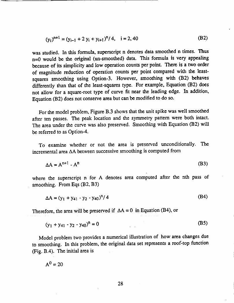
(yi) n+l = (Yi-1 + 2 Yi + Yi+l)n/4, i = 2, 40 032)

was studied. In this formula, superscript n denotes data smoothed n times. Thus

n=0 would be the original (un-smoothed) data. This formula is very appealing

because of its simplicity and low operation counts per point. There is a two order

of magnitude reduction of operation counts per point compared with the least-

squares smoothing using Option-3. However, smoothing with 032) behaves

differently than that of the least-squares type. For example, Equation 032) does

not allow for a square-root type of curve fit near the leading edge. In addition,

Equation 032) does not conserve area but can be modified to do so.

For the model problem, Figure B.3 shows that the unit spike was well smoothed

after ten passes. The peak location and the symmetry pattern were both intact.

The area under the curve was also preserved. Smoothing with Equation 032) will

be referred to as Option-4.

To examine whether or not the area is preserved unconditionally. The

incremental area AA between successive smoothing is computed from

AA = A n+l - A n 033)

where the superscript n for A denotes area computed after the nth pass of

smoothing. From Eqs 032, B3)

_A = (Yl + Y41 - Y2 - Y40)n/4 034)

Therefore, the area will be preserved if AA = 0 in Equation (B4), or

(Yl + Y41 - Y2 - Y40)n = 0 035)

Model problem two provides a numerical illustration of how area changes due

to smoothing. In this problem, the original data set represents a roof-top function

(Fig. B.4). The initial area is

A0 = 20

28

After ten passes of smoothing (Fig. B.4), the roof-top of the initial area has beensmoothed out and some area is lost. The area reduces to

AI°= 19.75

That is, each pass of smoothing results in an area change of

AA = - 0.025

For area conservation, the smoothing formula Equation (B2) must be modified

next to the end point at i = 2 and i - 40 by

(y2) n+l = (0.75 Y2 + 0.25 y3) n

(,Y40) n+l = (0.75 Y40 + 0.25 Y39)n

(B6)

With this modification, and using Equations (B2, B3) it can be shown that the area

is conserved. This weighted averaging smoothing procedure will be referred to as

Option-5. The special end point formula 036) can lead to non-smoothness next to

the end point. In Figure B.5 after one pass of smoothing, a slight kink shows up

next to either side of the end point. The kink gets much stronger by the tenth pass

of smoothing. The area lost near the roof-top has been offset by the area gained in

the vicinity of the kink.

It is undesirable to have a smoothing procedure that may introduce additional

kinks (non smoothness) into the data. Option-4 is chosen instead of option-5. The

area change is quite small if only a small number of smoothing passes are applied.

In addition, the real data usually has peaks and valleys and there may be a

cancellation effect between area gain and area loss. Asymptotic behavior of the

smoothing procedures is discussed below.

B.3 Asymptotic Behavior

When the smoothing formula is used successively and indefinitely, it is

interesting to note the asymptotic behavior of the formula. Let

29

Ayi = (yi)n+l _ (yi)n

When the iteration converges Ayi = 0, or

037)

(yi) n+l = (yi) n (B8)

For option 4, from Equations 032, B8)

(Yi-1 - 2 Yi + Yi+l)n = 0, i = 2, 40 039)

This condition can be satisfied if and only if the curve becomes a straight line

connecting the two end points.

For option 5, from Equations 032, B6, BS)

(Yi-l-2yi+Yi+l)n=0, i=3,39

0310)

(y2) n = (y3) n

(Y4O) n = (Y39)n

The converged curve becomes a trapezoid whose area equals that of the pre-

smoothed data. It is obvious that one should not attempt to converge the

smoothing iteration. In practice, the data is not as spiky as that of the model

problems, and a few passes (i. e., three to five) of smoothing are sufficient to arrive

at a smoothed curve.

30

p_

31

!

O

O _

o _o

_ O

ogll.q

0

c_

32

:::)

o_

c3

1_ c',,1I qp.,--I

!

s,--I !

p,,.¢

io iJ oo ow ol

.-1 ,.-1 ,-1

O

,-q e:_

I

b=

33

! 1

a) Regular Point

/

I 1 BLK2

b) Singular Point at Fictitious Edge

Figure 3. Regular and Singular Points at Block Boundaries.

34

O0

o

II,--q

",.._

o

0.,_

N"2

0Q.)

35

.o

I II,I

"0a)r- "00o_E o0_ 0c E

/

t

0 0

t_

0

0

5_00E

0w,,_

rj

36

llj

f _

!

0

37

l I ,

I,li

09 O9 COO. O. O_(D q) (D

00(009O O OO O OO4 _O uO

!//

////,/

/

//. ,)

/,I'l

'k. _.

I

c_o" O o o

O

U9

(5

"O

oo

II"

,-2I

_J

_J(J

Z

O

Z"O_J

0_

OoO

<J

O

_J

4)t_0

oc_

O£)

r_QJ

_0,e,,_

Lu

38

Nacelle-1 o

Nacelle-2

-0.5

co 0ooOOO o

0.0 .

0.5 ,).0 015 x/c 1.0

0.25

r/c

0.20

0.15

0.0

o

o

I

015 _c 1.0

Figure 8. Comparison of Cp and Geometries Between Two

Nacelles, M**=.85, c_=0 degrees.

39

0.5

0.0 015 x/c 1.0

0.25.

r/c

0.20

0.0!

ols x/c 1.o

Figure 9. Design of an Isolated Nacelle, M**=.85, _--0 degrees.

40

Cp

0000

Initial o

1st x2nd n

3rd4th o5th +6th z_

Target

oo '_ o15 x/c 11o

0.25

r/c

0.20

0.15!

0.0 015 _c 1.0

Figure 10. Convergence of Design Iterations for an Isolated

Nacelle, M0.=.85, oc=0 degrees.

41

!

_o

c_

42

0.

0.Q

0

Q. 0o ci

0'fill

"c_

0

c_

_ _ °×l

ci

0m w

qllml

_ w_ - v sII_ v

"o

!

0 0o ci

0

TII

"0

tr_

'cl

!d

c_z

r._

',- 0

d

0

0l.t")d

0

@

43

44

o o

0d

0

e_

8

"o

_oo°

0I ._

0d d

0 d

0

! •

0 0d d

0

o.

d

0d

o "_- °

_J

Z

An

t_o

4S

Cp

0.0

x

Initial °

1st x2nd []

3rd4th o5th +6th A

i m III

III

U

0.01

015 x/c 1.0

0.3

r/c

ti

II

III

%

0.2!

0.0 015 x/c 1.0

Figure 15. Convergence of Cp and Geometries in Installed Nacelle

Design, M0.=.77, oc=.5 degrees.

46

d d

o

d d d d

ii "• Lo

"- 0 " I_

o _o o dd d0

iz

47

o_ _,_,g__=o_o

c5 >, d 9"

0I-q

,<

× ._

0

0

o 0"- rJ

48

El--OTm

m _

O_

I

d _ d

oc_

x

o

!

c_!

o

49

0

E

0

•_ 0

_o

!

mar) od _,. d 9

x

<V

o=

b_

0

5O

x

<

I

0

C)

,.Q

C_

i,

51

0

X

0

!

g

8.

0

0

0

0

J

52

I Form Apprc. r.'JREPORT DOCUMENTATION PAGE OM8 ,,'oo.'c.:,_s_

_* AGENCY USE ONLY (L_clv_ b_r)k)I _1"_ _

4. TITLE AND SUBTITLE

An Inmll_d Nwelk Dest_ Cod_ U_Mg a MalfiblockEuI_' Solver, Volume I: Themy Dooa,nm_

6. AUTHOR(S)

H. Ca_

7. PERFORMING ORGANIZATION NAME(S) AND ADDRESS(/S)

P. O. Box 3707WA 98124-22O7

g. SPONSORff,IG/MONITORING AGENCY NAME(S) AND ADDRESC.(r..c)

3. REPORT TYPE AND DATES COVEREDO:mmmmt Re w_'5. FUNDING NUMBE/,.S

N.,_ 1-1r/03

_ Aermmuflcs and Space _L_SI_ _ C_.=_VA 236&S-_22.S

ORIGINAL P,_QE ISOF POOR QUALITY

B. PERFORMING ORGANIZATIONREPORT NUMBER

10. SPCP4SC_;N6 _,'r_'?,ITC,_,'4GAGENCY REFO&T I_L':/,6[ R

11. SUPPLEMENTARY NOTES

Langley Techn/cal Monlm_. Bobby L_

12a. DISTRIBUTION,AVAtL,_BILITY STATEMENT

Unc_ Unm_;_,_SubJect C_gory 02

12b. C.:ST,_IbUT_C', CCLE

13. ABSTRACT (t,_aximum 200 word_)

An _ mulfiblock Eulct dedl_ code was d_lopcd for d_igning a naceUc inmdi_d oaS_Y complex aL,pla_ ¢onfi_ TI_ _ mployod a d_ign drivot ba_ oaadirect ltm_v_ surface curvature mcth. od developed at NASA-Langley. A general mukiblocke,___ flow solver was _ for .computm.I_flow suound, comply. _. Thc flow sol v= useda .[_.l_-vomm_ formulation wire. explicit ume-stcppmg to solve me _,mcr equations. It _ •muldblock _mdon ot d,o m_dfllF'idmethod Io accclcratc the coavcrgeucc of the calculadoas. TI_de,sign dlivel" _voly Ul_..te_. the suffice geomelzy to n_luoe the differe_e _ the_mputed and ut_,et pressure dimil_dons. In the flow solver, the.clumge in surfacewas sire.ula_., by.apply_, g s.ufl'scc ttanspinuion boundm7 condit:mas to avoid _,zpeat_d _dl_..m_-o_ _ o_lm ttcrauons. Smoodmess of the dedB_d mrf_ce was mmmxl by al_appUcatk_ o_ mumwise and ci_u_e_n_ smoothinp. _ capabflky and effiency ofth_ codew•s (Immmmmsd dm:mght._ed_l_ oflx_ an bolmed mmolleand ,., im'_ed _lle m vmimmflow oa,m_a_._. _onumio_ Dotim exeaudonof _ oompumr _ is _ in Volum_ nwklch ;,, titled _m I_l_d Nacelle De._i_ Oa,deu_r_g • Mul_block Eu_ Solve. VoL n- Ue,otO,,;de'.

t4. SUBJECT TERMS

Nacelle Design. M_fibloch _ Code

17. SECURITY CLASSIFICATION | lB. SECURITY CLASSIFICATION | 19.

OF REPORT i OF THIS PAGE IUr=bssif_ Ur=l_,df_NSN 75"0-0 : -280-5500

SECURITY CLASSiFICATiONOF ABSTRACT

15. NUMBLR 0_ PAGES

16, PRICE CODL

20. LIMITA3tCN CI ABSTi, AC

S'P'C,_.'_ :.L'_'" ;')_ ',;:',:v 2£9: