c h a ra c te risin g a n d sim u la tin g ste lla r m ic ... · tu d e o f th e va ria tio n s c a...

Chapter 3

Characterising and simulating stellar

micro-variability

3.1 Introduction

The previous chapter focussed on the problem of transit detection, specifically in the

white Gaussian noise case, isolating other issues affecting any planet search project,

such as confusion and non-Gaussian noise sources. Tests of the algorithms presented

therein on simulated data have shown they can perform very well in white Gaussian

noise (as can other algorithms developed simultaneously or near-simultaneously by

other authors), reliably detecting transits and quantifying their statistical significance.

However, rather than the detection of the transits themselves, the major dif-

ficulty for ground-based searches so far has in fact been distinguishing planetary

transit-like events caused by stellar systems, such as eclipsing binaries with high mass

ratios, or hierarchical triple systems (due to either a physical triple system or an eclips-

ing binary blended with a foreground star), from true planetary transits (Brown 2003).

In order to detect terrestrial planets, it is necessary to go to space, to avoid

being affected by atmospheric scintillation and to monitor the target field(s) contin-

uously, with minimal interruptions. With improved photometric precision comes an

additional noise source, which is usually insignificant at the precisions achieved by

ground based observations: the intrinsic variability of the stars, due mainly to the

temporal evolution and rotational modulation of structures on the stellar disk. The

Sun’s total irradiance (see Figure 3.1) varies on all timescales covered by the avail-

able data, with a complex, non-white power spectrum (see Figure 3.3). The ampli-

tude of the variations can reach more than 1 % when a large spot crosses the solar

disk at activity maximum, compared to transit depths of tenths to hundredths of a

percent. There is significant power on timescales of a few hours, similar to the typi-

86 Characterising and simulating stellar micro-variability

cal transit duration. Untreated, solar micro-variability would significantly reduce the

detection performance of missions such as Eddington or Kepler (see Section 2.1.4),

while the variability levels of more active stars are expected to also affect COROT

and even ground-based transit searches in young stellar environments.

However, it is possible to separate planetary transit signal and stellar variability

because the former is of relatively well known shape and contains significant power

at high frequencies, while the latter is concentrated mainly at low frequencies. Al-

ready, modified transit search algorithms, designed to distinguish between the transit

and brightness variations of stellar origin, have been tested on simulated data in-

cluding solar variability (Defay et al. 2001; Jenkins 2002). Jenkins (2002) applied a

simple scaling to the solar irradiance data to evaluate the impact of increased ro-

tation rate. Nonetheless, a more physical model, in which the different phenomena

involved can be scaled independently in timescale and amplitude for a range of

spectral types and ages, is needed to simulate realistic light curves for stars other

than the Sun. This will allow us to optimise, evaluate and compare different algo-

rithms, but also different design and target field options for the space missions con-

cerned.

The present chapter is concerned with the development of such a model.

The philosophy adopted in the process is the following. Intrinsic stellar variability is

by no means a well-understood process. Despite recent progress in the modelling

of activity-induced irradiance variations on timescales of days to weeks in the Sun

(Krivova et al. 2003; Lanza et al. 2003), the extension of these physical models to other

stars remains problematic, due to the scarcity of information on how the timescales,

filling factors of various surface structures, and contrast ratios, depend on stellar pa-

rameters. We have therefore adopted an empirical approach, using chromospheric

flux measurements as a proxy measure of activity-induced variability. This step is pos-

sible due to the fact that a correlation between the two quantities is observed in the

Sun throughout its activity cycle, as well as in other stars. Similarly, empirically de-

rived relationships were used again to relate chromospheric activity, rotation, age

and colour, rather than attempting to use models which make a number of assump-

tions about the physical process driving these phenomena, and generally depend

on parameters which require fine-tuning.

The stellar micro-variability model is developed by extrapolating the results of a

detailed Fourier analysis of total solar irradiance (TSI) variations (Section 3.2) to other

spectral types and stellar ages through empirical scaling laws (Section 3.3). Tests of

the model are presented in Section 3.4. The results are discussed in Section 3.5

3.2 Clues from solar irradiance variations 87

a)

0 500 1000 1500time (days)

1354

1356

1358

1360

1362

1364

1366

flux

(W/m

2 )b)

0 500 1000 1500time (days)

0.9985

0.9990

0.9995

1.0000

1.0005

1.0010

norm

alise

d flu

x

Figure 3.1: PMO6 light curve, a) before and b) after the pre-processing steps described inSection 3.2.1.1. The data starts in January 1996.

3.2 Clues from solar irradiance variations

The Sun is the only star observed with sufficient precision and frequent sampling to

permit detailed micro-variability studies, thanks to the recent wealth of data col-

lected by the SoHO spacecraft, and particularly the full disk observations obtained

by VIRGO (Variability of solar IRradiance and Gravity Oscillations), the experiment for

helioseismology and solar irradiance monitoring on SoHO, (Frohlich et al. 1997).

Stellar micro-variability is difficult to observe from the ground due to its very low

amplitude, except for very young, active stars – which are outside the main range of

interest for planet searches. There is some information available on rms night-to-night

and year-to-year photometric variability of a small sample of stars monitored over

many years by a few teams (Radick et al. 1998; Henry et al. 2000b). We make use

of these as they present the advantage of covering a range of stellar ages, but their

irregular time coverage and limited photometric precision make them unsuitable for

an in-depth study, and particularly for the detailed analysis of the frequency content

of the variations.

A drastic improvement in our understanding of intrinsic stellar variability across

the HR diagram is expected from the very missions this work is aimed at preparing. In

the relatively short term, MOST will provide valuable information for a small sample of

stars, but it is not until the launch of COROT, and later Kepler and Eddington, that a

wide range of stellar parameters will be covered. In the mean time, we must make

use of the detailed solar data, and make reasonable assumptions to extrapolate to

other stars than the Sun.


Powe

r per

uni

t fre

quen

cy(fr

actio

n of

tota

l)

Figure 3.2: Cumulative power spectrum ofthe PMO6 light curve after pre-processing,as a fraction of the total power at non-zero frequencies. The grey area showsthe range of frequencies corresponding totypical transit durations (2 to 15 hrs). Over95 % of the power in the solar variations isbelow that range, which suggests that thetwo types of signal can be separated onthe basis of their frequency signature.

3.2.1 SoHO/VIRGO total irradiance (PMO6) data

All SoHO/VIRGO data used in this work were kindly provided by the VIRGO team

at ESTEC. The main instrument of interest was PMO6, a radiometer measuring total

solar irradiance. The light-curves used here cover the period January 1996 to March

20011, which roughly corresponds to the rising phase of cycle 23.

3.2.1.1 Pre-processing of the data

The light curves were originally received as level 1 data, in physical units but with

no correction for instrumental effects. Careful treatment was required to remove

long term trends of instrumental and astrophysical origin. There was a difference

of ∼ 0.24 % in the mean measured flux between the start and the end of the time

series. Given that the observations roughly correspond to the interval between the

minimum and the maximum of the Sun’s activity cycle, one might expect to see a rise

in the mean irradiance over that period. The instrumental decay may therefore be

higher than the value quoted. However, the absolute value of the irradiance was of

little interest for the present study, which concentrates on relative variations on time

scales of weeks or less. Any long term trends in the data were therefore removed

completely, regardless of whether they were of instrumental or physical origin2. The

decay appeared non-linear and there were discontinuities and outliers in the light

curves, making a simple spline fit unsuitable.

The approach that was adopted consisted of a 5 step process:

1Except for two interruptions roughly 1,000 days after the start of operations, corresponding to the“SoHO vacations”, when the satellite was lost and then recovered.

2Note that fully corrected (level 2) data are now freely available from the World Radiation Centre inDavos, Switzerland for the period March 1996 to December 2002 (for data with minute sampling, morerecent data is available with hourly sampling). Level 2 data is corrected for instrumental effects butcontains the long-term trends due to the solar activity cycle. As only trends on timescales of 2 monthsor less were of interest here, the relatively crude corrections we applied to the level 1 data ourselveswere sufficient.


• Visual inspection of the data was used to manually remove sections visibly af-

fected by instrumental problems.

• Spline fits were performed on intervals chosen by visual inspection to start and

end where discontinuities occurred. Each interval was divided by the corre-

sponding fit, resulting in a normalised output light curve.

• A 5 σ cutoff was applied for outlier removal.

• The sampling, originally 1 min, was reduced to 15 min to make the size of the

light curves more manageable. This was done by taking the mean of the orig-

inal data points in each 15 min bin, ignoring any missing or bad data points. It

is unlikely any information on timescales shorter than 15 min would significantly

impact the transit detection process, as the transits of interest here generally

last several hours (corresponding to orbital periods of several months or years).

• Data gaps were replaced with the baseline value of 1.0, to allow the calcula-

tion of the amplitude spectra needed for the analysis3.

3.2.2 Modelling the ‘solar background’

Table 3.1: Typical timescales for the differ-ent components of the solar background.

Component Timescale B (s)

Active regions 1 to 3 × 107

Super-granulation 3 to 7 × 104

Meso-granulation # 8000Granulation 200 to 500Bright points # 70

The power spectrum of the solar irradiance variations at frequencies lower than

# 8 mHz constitutes a noise source for helioseismology, usually referred to as the ‘solar

background’. It is common practice to fit this background with a sum of powerlaws

in order to model it accurately enough to allow the measurement of solar oscilla-

tion frequencies and amplitudes. Powerlaw models were first introduced by Harvey

(1985). The most commonly used model in the literature today is that of Andersen

et al. (1994), which is fairly similar: the total power spectrum is approximated by a

sum of power laws, the number N of which varies between three and five depend-

3If di is a regularly sampled dataset, the dataset in which gaps have been replaced by 1.0 is d′i =

di ∗ wi + 1 − wi , where wi is window function, i.e. is 0 in the gaps and 1 elsewhere. The FT of d′i is then,

for all non zero indices k , D′k = Dk ! Wk − Wk , where Dk and Wk are the FTs of di and Wi respectively.


a)

0.1 1.0 10.0 100.0frequency (µHz)

10-9

10-8

10-7

10-6

10-5

10-4

powe

r ((W

/m2 )2 H

z-1)

b)

500 1000 1500time (days)

0

2•10-5

4•10-5

6•10-5

8•10-5

powe

r ((W

/m2 )2 H

z-1)

pow

er (n

orm

. flu

x sq

uare

d)

pow

er (n

orm

. flu

x sq

uare

d)

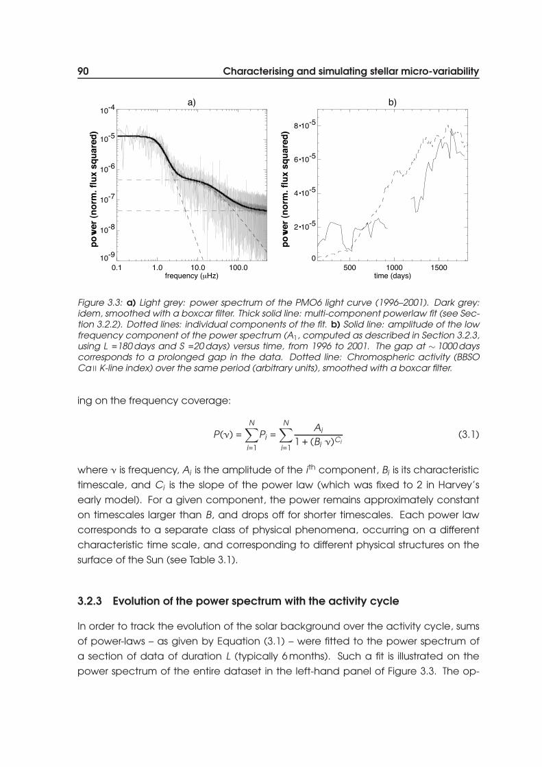
Figure 3.3: a) Light grey: power spectrum of the PMO6 light curve (1996–2001). Dark grey:idem, smoothed with a boxcar filter. Thick solid line: multi-component powerlaw fit (see Sec-tion 3.2.2). Dotted lines: individual components of the fit. b) Solid line: amplitude of the lowfrequency component of the power spectrum (A1, computed as described in Section 3.2.3,using L =180 days and S =20 days) versus time, from 1996 to 2001. The gap at ∼ 1000 dayscorresponds to a prolonged gap in the data. Dotted line: Chromospheric activity (BBSOCa II K-line index) over the same period (arbitrary units), smoothed with a boxcar filter.

ing on the frequency coverage:

P(ν) =N∑

i=1

Pi =N∑

i=1

Ai

1 + (Bi ν)Ci(3.1)

where ν is frequency, Ai is the amplitude of the i th component, Bi is its characteristic

timescale, and Ci is the slope of the power law (which was fixed to 2 in Harvey’s

early model). For a given component, the power remains approximately constant

on timescales larger than B, and drops off for shorter timescales. Each power law

corresponds to a separate class of physical phenomena, occurring on a different

characteristic time scale, and corresponding to different physical structures on the

surface of the Sun (see Table 3.1).

3.2.3 Evolution of the power spectrum with the activity cycle

In order to track the evolution of the solar background over the activity cycle, sums

of power-laws – as given by Equation (3.1) – were fitted to the power spectrum of

a section of data of duration L (typically 6 months). Such a fit is illustrated on the

power spectrum of the entire dataset in the left-hand panel of Figure 3.3. The op-


0 20 40 60 80 100BBSO CaII K-line index

0

2•10-5

4•10-5

6•10-5

8•10-5

A 1 (P

MO

6)

Figure 3.4: Amplitude A1 of the low fre-quency component of the solar powerspectrum (computed as described inSection 3.2.3, using L =180 days andS =20 days), versus the BBSO Ca II K-line in-dex (arbitrary units) over the period 1996to 2001.

eration is then repeated for a section shifted by a small interval S from the previous

one (typically 20 days), and so on. Thus the evolution of each component can be

tracked throughout the rise from solar minimum (1996) to maximum (2001) by mea-

suring changes in the parameters defining each powerlaw.

A single component fit with parameters A1, B1 & C1 is made first. Additional

components are then added until they no longer improve the fit, i.e. until the addition

of an extra component does not reduce the χ2 by more than 10−2. The fit to the

first section is used as the initial guess for the fit to the next section, and so forth. This

method allows us to track the emergence of components corresponding to different

types of surface structures throughout the solar cycle, as well as monitor variations in

amplitude, timescale and slope for each component.

3.2.3.1 Results

The algorithm described above was run on the PMO6 data with L = 180 days and

S = 20 days, and three components were found to provide the best fit in all cases.

These components have stable timescales and slope, varying in amplitude only. The

physical processes giving rise to each component are thus of a permanent nature.

A number of points of interest emerge from the results. The first component, with

τ # 1.3 × 105 s (active regions) shows an increasing trend in amplitude which is well

correlated with the Ca II K-line index, an indicator of chromospheric activity. This is

illustrated in the right-hand panel of Figure 3.3. The slope of the powerlaw is 3.8 (in

good agreement with Andersen et al. 1998).


The observed correlation, which is further illustrated by the scatter plot in Fig-

ure 3.4, comes as no surprise. The passage of individual active regions across the

disks of the Sun and other stars monitored by the Mt Wilson HK Project can be clearly

seen in plots of the activity index S (from which R ′HK is derived) versus time4. On the

other hand, the effect of the same type of event on the solar irradiance has been

studied with a number of instruments, most recently VIRGO/LOI and PMO6 (Domingo

et al. 1998). Recent models including contributions from faculae and sunspots of tun-

able size and number reproduce the PMO6 light curve to a high degree of precision

(Krivova et al. 2003; Lanza et al. 2003).

However, observing and characterising a correlation throughout the Sun’s ac-

tivity cycle, between a chromospheric activity indicator which can be measured

from the ground for a large number of stars, and total irradiance variations, whose

amplitudes are so small they are only observable by dedicated high-precision pho-

tometric space missions, goes one step further. Most importantly for planetary transit

searches, it implies that chromospheric activity indicators such as R ′HK can be used

as a proxy to predict weeks timescale variability levels for a wide range of stars.

The amplitude of the second component also increases, but is not correlated

to the Ca II index. This component corresponds to timescales corresponding to

super- and meso- granulation, for which no detailed models are available to date.

Our understanding of this kind of phenomenon is expected to improve dramatically

when the results from space-based experiments designed for precision time-series

photometry will become available.

3.2.3.2 Implications

The correlation between A1 and the Ca II K-line index, although not extremely tight, is

a clear indication that chromospheric activity indicators contain information about

the variability level of the Sun on timescales longer than a few days. To establish more

solidly a scaling law between photometric variability and chromospheric activity, we

must use a wider stellar sample to constrain the relation over the entire expected

range of activity levels (see Section 3.3.1.3).

Little useful information has been extracted from the solar data on what deter-

mines the parameters of the solar background other than A1. The few clues available

from other sources will be presented in Section 3.3.2.

4See the Mt Wilson HK project homepage, http://www.mtwilson.edu/Science/HK Project/.

3.3 Empirical scaling to other stars 93

3.3 Empirical scaling to other stars

The main aim of the present model is the simulation of realistic light curves of stars

more active than the Sun, if possible as a function of stellar parameters such as spec-

tral type and age, via observables such as B−V colour and rotational period Prot. The

multi-component power-law model used in Section 3.2 to fit the solar background

power spectrum now forms the basis of the simulation of enhanced variability light

curves.

To simulate a light curve for a given star, the first task is to generate a power

spectrum using this power-law model. When applying the component-by-component

procedure described in Section 3.2.3 to fit solar power spectra, the optimal number

of components was found to be three. We therefore use a sum of three power-laws

to generate the stellar power spectra. The highest frequency component, a super-

position of granulation, oscillations and white noise, has a characteristic timescale

which is shorter than the typical sampling time for planetary transit searches, and

thus can be replaced by a constant value(i.e. a random noise component). There

are therefore a total of 7 parameters to adjust for each simulated power spectrum:

three for each resolved power-law plus one constant.

The inputs of the model are the spectral type and age of the star. Starting from

these theoretical quantities given, how are the power-law parameters deduced?

Most of the information available concerns the amplitude of the first power-law, A1.

The scaling of this parameter is described in detail in Section 3.3.1, while that of the

other parameters of the model, whose treatment is much simpler, is discussed in

Section 3.3.2.

3.3.1 The amplitude of the active regions component

We have established in Section 3.2 that there is a correlation between A1 and the

Ca II K-line indicator of chromospheric activity in the Sun. We will see in this section

that such a correlation holds for a wide stellar sample. On the other hand, there is

a well known scaling between rotation period, colour and chromospheric activity

(Noyes et al. 1984). Provided one can estimate the rotation period of the star (Sec-

tion 3.3.1.1), the activity level can be computed (Section 3.3.1.2), and from this one

obtains A1 (Section 3.3.1.3).

3.3.1.1 The rotation period-colour-age relation

As detailed in Section 3.3.1.2, it is possible to deduce the expected activity level for

a star of known mass (i.e. colour) and rotation period. However, the number of stars


with known rotation periods is relatively small. In the context of the present work, it

would thus be useful to be able to predict the rotation period for a given stellar mass

and age.

Observational constraints on rotation rates for stars of known mass and age

come from two sources: star forming regions and young open clusters, where one

can measure photometric rotation periods or rotational line broadening (v sin i); and

the Sun itself. There is little else, as rotational measurements are hard to perform

for all the quiet, slowly rotating intermediate age and old stars other than the Sun,

except for relatively nearby field stars, for which little reliable age information is avail-

able. The status of observational evidence and theoretical modelling in this domain

is outlined by Krishnamurthi et al. (1997), Bouvier et al. (1997) and Stassun & Terndrup

(2003). Here we briefly sketch the current paradigm to set the context of the present

work.

The observed initial spread in rotation velocities (from measurements of T-Tauri

stars, with a concentration around 10–30 km s−1 but a number of fast rotators, up to

100’s of km s−1) is attributed to the competing effects of spin-up (due to the star’s

contraction and accretion of angular momentum from the disk) and slowing-down

mechanisms such as disk-locking (Konigl 1991; Bouvier et al. 1997). This spread is ob-

served to diminish with age (by the age of the Hyades, only some M-dwarfs still exhibit

fast rotation, Prosser et al. 1995), leading to a dependency of rotation on mass only.

Following this homogenisation, one observes constant spin-down in a given mass

range. For example, Skumanich (1972), comparing rotational velocities Sun-like (G)

stars in the Pleıades, the Hyades and for the Sun, found them to decay as the square

root of age, implying that the rotation period of of main sequence Sun-like stars in-

creases as t1/2 where t is the age on the main sequence. Both homogenisation and

power-law spin-down can be explained by the loss of angular momentum through

a magnetised wind (Schatzman 1962; Weber & Davis 1967), a mechanism which is

more effective in faster rotators.

Angular momentum evolution models have vastly improved recently, but they

still rely on the careful tuning of a number of parameters, especially for young and

low-mass stars. We have therefore chosen to use empirically derived scaling laws

and to restrict ourselves to the range of ages (older than the Hyades) and spectral

types (mid-F to mid-K) where a unique colour-age-rotation relation can be estab-

lished. In this range the aforementioned parameters become less relevant and the

models reproduce the observations fairly robustly.

A relationship between B−V colour (i.e. mass) and rotation at a given age was

empirically derived from photometric rotation period measurements in the Hyades

(Radick et al. 1987, 1995). Only rotation periods were used, rather than v sin i mea-


0.4 0.6 0.8 1.0 1.2 1.4(B-V)

0.2

0.4

0.6

0.8

1.0

1.2

1.4

1.6

log(

P rot)

34567 Figure 3.5: Plot of rotation period versus

B − V colour for Hyades stars. Data fromRadick et al. (1987, 1995). The thin par-allel black lines correspond to ‘rotationalisochrones’ from Kawaler (1989) with t asindicated next to each line (in units of108 yr). The dashed line is a linear fit to thedata with 0.6 ≤ B − V < 1.3. The thick solidline is a composite of two linear fits, one forB−V < 0.62 and one for 0.62 ≤ B−V < 1.3.

surements, to avoid introducing the extra uncertainty of assigning random inclina-

tions to the stars and having to assume theoretical radii to convert v sin i to a pe-

riod. This relationship is valid for the range 0.45 ≤ B − V ≤ 1.3. For stars bluer than

B − V = 0.45, rotation rates saturate, but this is outside the range of spectral types of

interest for the present work. Redder than B − V = 1.3, a significant spread is still ob-

served in the rotation periods. The remaining range is divided into two zones, each

following a linear trend. Redder than B − V = 0.62, the slope of the relation is quite

close to the theoretical relation obtained by Kawaler (1989). We also estimated the

age of the Hyades from the zero-point of the linear fit as done by Kawaler (1989), but

incorporating the improved data from Radick et al. (1995). The age obtained in this

manner is 634 Myr, consistent with recent determinations by independent methods:

655 Myr (Cayrel de Strobel 1990), 600 Myr (Torres et al. 1997), and 625 Myr (Perryman

et al. 1998), thereby confirming the quality of the fit. The slope for stars bluer than

B − V = 0.62 is much steeper, presumably due to the thinner convective envelopes

of the stars in this range.

This can then be combined with the t1/2 spin-down law into a rotation-colour-

age relation:

log (Prot) − 0.5 log(

t625 Myr

)={

−0.669 + 2.580 (B − V ), 0.45 ≤ B − V < 0.62

0.725 + 0.326 (B − V ), 0.62 ≤ B − V < 1.30

} (3.2)

A comment on the adopted value of 0.5 for nt , the index in the spin-down law


is appropriate. It has recently been suggested that a value of 0.6 might be more

appropriate (Guinan & Ribas 2002, on the basis of an updated sample of Sun-like

stars with some new age determinations). However, the original value of 0.5 was

kept for the present work. The change would not affect the predicted rotation rates

significantly, and the errors on this new value of nt (which depends, for example,

on age determinations from isochrone fitting) are larger than the difference. We

have therefore kept the lower value, as it leads, if in error, to overestimated rotation

rates, hence more variability and on faster timescales, and eventually conservative

estimates of transit detection rates.

3.3.1.2 The activity-rotation period-colour relation

The next step consists in estimating from the colour and rotation period the expected

chromospheric activity level of the star. For this purpose, the scaling law first derived

by Noyes (1983) and Noyes et al. (1984) is used. It relates the mean Ca II index⟨R ′

HK

⟩to the inverse of the Rossby number Ro, and can thus be understood in terms of the

interplay between convection, rotation and the star’s dynamo:

− log Ro = 0.324 − 0.400 y + 0.283 y2 − 1.325 y3 (3.3)

where y = log⟨R ′

HK

⟩5

and⟨R ′

HK

⟩5

=⟨R ′

HK

⟩× 105. Ro is related to the rotation period Prot

and B − V colour as follows:

Ro = τc/Prot (3.4)

where Prot is expressed in days, and the following (empirically derived) relation for τc,

the convective overturn time, is used:

log (τc) ={1.361 − 0.166 x + 0.025 x2 − 5.323 x3, x ≥ 0

1.361 − 0.140 x , x < 0

}(3.5)

where x = 1 − (B − V ). Equation (3.3) was inverted (using an interpolation between

tabulated values) to allow us to deduce the chromospheric activity index from the

rotation period and B − V colour of a star. For details of how the above relations,

which are simply stated here, were obtained, the reader is referred to Noyes et al.

(1984).


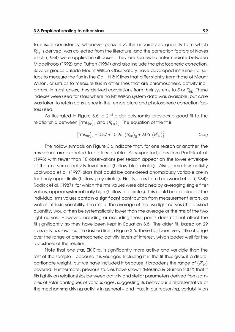
Figure 3.6: Photometric variability[rmsby

]4

versus chromospheric activity⟨R′

HK

⟩5

for72 field and Hyades stars. The colourcoding refers to the source of the pho-tometric variability data. Green: Henryet al. (2000b). Blue: Radick et al. (1998)(hollow: <10 observations per season).Grey: Lockwood et al. (1997) (hollow:rmsby ≤2 mmag, upper limits only). Red:Hyades stars (filled: Radick et al. 1995, hol-low: averages of rmsb & rmsy from Lock-wood et al. 1984 & Radick et al. 1987).Solid line: 2nd order polynomial fit to thedata. Dashed line: relation used in Aigrainet al. (2004), based on 29 stars only.

3.3.1.3 Active regions variability and chromospheric activity

Having noted that the ‘active regions’ component of the solar activity spectrum ap-

pears directly correlated to chromospheric activity (see Section 3.2.3), we turn to the

small but valuable datasets containing both photometric variability measurements

and activity indexes for a variety of stars. The data available on any one star is of

course much less precise and less reliable than the solar data, but the dataset as a

whole spans a much wider range of activity levels.

We use a sample of stars for which both⟨R ′

HK

⟩and photometric variability mea-

surements are available in the literature. In Aigrain et al. (2004), we restricted our-

selves to 29 stars whose variability levels and chromospheric activity indices were

published in the same papers, namely Radick et al. (1998); Henry et al. (2000b).

These data were then used to derive a quantitative relationship between⟨R ′

HK

⟩4

and

the night-to-night rms variability in Stromgren b and y ([rmsby

]4

= rms{(b+y)/2}×104,

in magnitude units).

Since then, a wider literature search has revealed a number of additional stars

for which photometric variability and chromospheric activity information were avail-

able, but in separate sources: additional photometric variability data were taken

from Lockwood et al. (1984); Radick et al. (1987, 1995); Lockwood et al. (1997), while

activity data, when not found in the above sources, were taken from Barry et al.

(1987); Duncan et al. (1991); Garcia-Lopez et al. (1993); Baliunas et al. (1995). The full

sample, illustrated in Figure 3.6, now contains 72 stars.

At the same time as including the additional data in the calibration, additional

care was taken to ensure consistency between datasets from different sources and


to minimise systematic errors.

Variability measurements

• Sparse time sampling: Some of the sources used, for example Radick et al.

(1998), were mainly designed to study long term variations (similar to the Sun’s

activity cycle) and their observations were rather sparse, sometimes counting

as few as 5 or 6 points per observing season. This could lead to an underes-

timate of, or in any case a larger uncertainty in, the short-term (night-to-night

within 1 season) rms values, which were those used in Aigrain et al. (2004). In

order to limit the impact of sparse time sampling, the average of night-to-night

rms values from different observing seasons was used, including only seasons

with more than ten observations whenever the number of observations per sea-

sons was given. Lockwood et al. (1997) and Radick et al. (1998) gave only the

total number of observations and the number of seasons. For those, stars for

which the ratio of the two was less than 10 were flagged, to see if these ap-

peared systematically less variable than stars observed more frequently.

• Exclusions: As was done in Aigrain et al. (2004), HD 95735, which was monitored

by Henry et al. (2000b), was excluded from the analysis as it lies outside the

range of B − V colours considered in the model.

• Sensitivity limits: In the case of data from Lockwood et al. (1997), it should be

noted that rms values ≤ 17 mmag are at the detection limit for variability and

should be considered as upper limits only.

• Filters: Lockwood et al. (1984) and Radick et al. (1987) published b & y rms

values separately. In later papers they noted the great similarity between the b

& y light curves and averaged the two before computing rms values to improve

precision. In the present work, when including data from Lockwood et al. (1984)

and Radick et al. (1987), the average of the b and y rms values was used.

These stars were also flagged, to highlight the fact that the rms values were not

obtained in a totally consistent way with the others.

• Multiple appearances of a given star: When a given star was present in more

than one source, the latest source with more than 10 observations per season

was used.

Chromospheric activity measurements It is appropriate to mention here some pre-

cautions that were taken in the compilation of chromospheric activity index val-

ues. Two formulae for the temperature correction factor are commonly used (Mid-

delkoop 1992; Rutten 1984), and published R ′HK values have been derived with both.


To ensure consistency, whenever possible S, the uncorrected quantity from which

R ′HK is derived, was collected from the literature, and the correction factors of Noyes

et al. (1984) were applied in all cases. They are somewhat intermediate between

Middelkoop (1992) and Rutten (1984) and also include the photospheric correction.

Several groups outside Mount Wilson Observatory have developed instrumental se-

tups to measure the flux in the Ca II H & K lines that differ slightly from those of Mount

Wilson, or setups to measure flux in other lines that are chromospheric activity indi-

cators. In most cases, they derived conversions from their systems to S or R ′HK. These

indexes were used for stars where no Mt Wilson system data was available, but care

was taken to retain consistency in the temperature and photospheric correction fac-

tors used.

As illustrated in Figure 3.6, a 2nd order polynomial provides a good fit to the

relationship between[rmsby

]4

and⟨R ′

HK

⟩5. The equation of the fit is:

[rmsby

]4

= 0.87 + 10.96⟨R ′

HK

⟩5

+ 2.06⟨R ′

HK

⟩25

(3.6)

The hollow symbols on Figure 3.6 indicate that, for one reason or another, the

rms values are expected to be less reliable. As suspected, stars from Radick et al.

(1998) with fewer than 10 observations per season appear on the lower envelope

of the rms versus activity level trend (hollow blue circles). Also, some low activity

Lockwood et al. (1997) stars that could be considered anomalously variable are in

fact only upper limits (hollow grey circles). Finally, stars from Lockwood et al. (1984);

Radick et al. (1987), for which the rms values were obtained by averaging single filter

values, appear systematically high (hollow red circles). This could be explained if the

individual rms values contain a significant contribution from measurement errors, as

well as intrinsic variability. The rms of the average of the two light curves (the desired

quantity) would then be systematically lower than the average of the rms of the two

light curves. However, including or excluding these points does not not affect the

fit significantly, so they have been kept in Equation 3.6. The older fit, based on 29

stars only, is shown as the dashed line in Figure 3.6. There has been very little change

over the range of chromospheric activity levels of interest, which bodes well for the

robustness of the relation.

Note that one star, EK Dra, is significantly more active and variable than the

rest of the sample – because it is younger. Including it in the fit thus gives it a dispro-

portionate weight, but we have included it because it broadens the range of⟨R ′

HK

⟩covered. Furthermore, previous studies have shown (Messina & Guinan 2002) that it

fits tightly on relationships between activity and stellar parameters derived from sam-

ples of solar analogues of various ages, suggesting its behaviour is representative of

the mechanisms driving activity in general – and thus, in our reasoning, variability on


the timescales under consideration.

To be usable for our purposes, Equation (3.6) must be completed by a relation-

ship between[rmsby

]4

and A1. The desired value of A1 corresponds to white light

relative flux variations, not b and y magnitude variations. To obtain the rms of the

relative flux variations one must multiply the rms of the magnitude variations by a

constant factor of 2.5/ ln(10) = 1.08. This must then be converted to a white light

flux rms value. This requires the definition of a reference point in the solar cycle, at

which to compare the variability levels in the two bandpasses. Radick et al. (1998)

quote a single log⟨R ′

HK

⟩value of −4.89 for the Sun, which is an average of mea-

surements performed over many years. This defines a reference solar activity level,

corresponding roughly to a third of the way into the rising phase of cycle 23. The

average night-to-night variability as measured in b and y by Radick et al. (1998)

is rmsby = 5 × 10−4 mag. The corresponding white light variability level, measured

from a 6 month long section of PMO6 data downgraded to 1 day sampling, centred

on the date for which the measured activity level was equal to the reference level

defined above, is rmswhite ≈ 1.8 × 10−4 mag.

This allows us to convert from rmsby in magnitudes to rmswhite in relative flux. As-

suming a straightforward proportionality relationship the conversion factor is 2.78. This

conversion introduces a significant error in the overall conversion, as we observed

that the dependency of rmswhite on R ′HK (in the Sun) is slightly different in shape to

that of rmsby on⟨R ′

HK

⟩(in the stellar sample), so a proportionality factor is inaccurate.

However, until other stellar photometric time series that are sufficiently regular to per-

form the fitting process described in Section3.2.3 are available, it is the best we can

do. Finally one must convert from rmswhite to A1. As expected, a linear relationship

between these quantities as computed for the Sun is observed, yielding an overall

conversion between[rmsby

]4

and A1:

A1 × 105 = −0.24 + 0.66[rmsby

]4

(3.7)

Equation (3.6) thus becomes:

A1 × 105 = 0.33 + 7.23⟨R ′

HK

⟩5

+ 1.36⟨R ′

HK

⟩25

(3.8)

As space-based time-series photometric missions come online, we will be able

to calibrate the relations above with more and more stars. Amongst these missions

which have already provided useful data or will start doing so very soon are MOST

(Micro-variability and Oscillations of Stars, Walker et al. 2003), a small Canadian mis-

sion which saw first light on 20 July 2003, and the OMC (Optical Monitor Camera,

Gimenez et al. 1999) on board ESA’s new γ-ray observatory INTEGRAL. In the longer


term, COROT will also provide a wealth of information on stellar micro-variability.

These new data will allow us to calibrate the relations above with a wider va-

riety of stars. In particular, chromospheric activity and rotational period measure-

ments are available for a relatively large number of bright late type stars (Henry

et al. 1996; Baliunas et al. 1996; Radick et al. 1998; Henry et al. 2000b; Tinney et al.

2002; Paulson et al. 2002). If any of these are observed by the missions listed above,

yielding variability measurements, they will be incorporated in the present model.

3.3.2 Other parameters of the model

The previous sections were concerned with providing an estimate of one of the

model’s parameters, A1, given a star’s age and colour. However, there are a total

of 7 parameters to adjust. We have so little information on the super- and meso-

granulation component in stars other than the Sun that we have chosen, for now, to

leave it unchanged in the simulations, using the solar values.

3.3.2.1 The third component: timescales of minutes or less

The third (highest frequency) component observed in the Sun is a superposition of

variability on timescales of a few minutes, which is thought to be related to gran-

ulation, and higher frequency effects such as oscillations and photon noise. The

distinction between these effects is not resolved at the time sampling used for the

present study. There is very little information at the present time on equivalent phe-

nomena in other stars than the Sun (see below). Solar values were therefore used in

all simulated light curves for this component. Given the low amplitude of this com-

ponent, and the fact that it corresponds to timescales significantly shorter than the

duration of planetary transits, it should not affect transit detection significantly.

Granulation can be traced by studying asymmetries in line bisectors, leading to

the possible exploration of this phenomenon across the HR diagram (see for exam-

ple Gray & Nagel 1989). Trampedach et al. (1998), who modelled the granulation

signal for the Sun, α Cen A and Procyon, obtained very similar power and velocity

spectra for the three stars, despite the fact that convection is much more intense on

Procyon. Although very preliminary, these results suggest that the granulation power

may change only slowly with stellar parameters, thus supporting the use of the solar

values in the present model.


3.3.2.2 The second component: hours timescale

Again, solar values were used for all simulated light curves for this component. Work is

underway to identify the types of surface structures giving rise to the hours-timescale

variability in the Sun (Fligge et al. 2000), and the launch of the COROT mission will pro-

vide a dataset ideally suited to improving our understanding of this type of variability.

Keeping the super- and/or meso-granulation component identical to the solar case

is certainly an oversimplification, and it is the area where most effort will be focused

in the future, as it is highly relevant to transit detection, being on timescales similar to

transits.

The possibility of measuring the power spectrum of stochastic luminosity varia-

tions in stars other than the Sun on timescales of minutes to hours, using existing data

from the star-tracker camera of NASA’s WIRE (Wide Field Infrared Explorer), is also

under investigation5. However, difficulties associated with non-Gaussian noise and

frequent data gaps both short and long, have impeded such a measurement so far

(see Section 3.4.3.4).

3.3.2.3 Timescale of the (first) active regions component

Two parameters remain for the active regions component. We have kept the slope

of the power law, C1, unchanged from the solar case. Changing it slightly does not

seem to affect the appearance of the light curve significantly. More crucial is the

timescale B1.

If the active regions component of micro-variability is the result of the rotational

modulation of active regions, we expect B1 to be directly related to the period. How-

ever, the value obtained for the Sun is B1 = 8.5 × 106 s, i.e. 9.84 days, compared to a

rotational period of ≈ 26 days. This suggests that the timescale is not (or not exclu-

sively) dominated by rotational modulation of active regions, but by the emergence

and disappearance of the structures composing the active regions. Individual ac-

tive regions evolve on a timescale of weeks to months in the Sun (Radick et al. 1998),

but spots and faculae evolve faster: observed sunspot lifetimes range roughly be-

tween 10 days and 2 months (Hiremath 2002). We therefore deduce that sunspot

evolution is the process which determines B1 in the Sun.

One can in fact interpret the observed timescale purely in terms of rotational

modulation: the transit of a given spot across the solar disk would last half the rotation

period only, so that, given the shape of a sunspot transit signature, pure rotational

modulation could contribute to signal on timescales as short as a third of the rotation

5This data has already been used to perform asteroseismology on a number of bright stars (Schou &Buzasi 2001) following the failure of the main instrument shortly after launch.


Prot (days)

P rot

B1

B1solar

10 27

solarperiod

starspotlifetimes

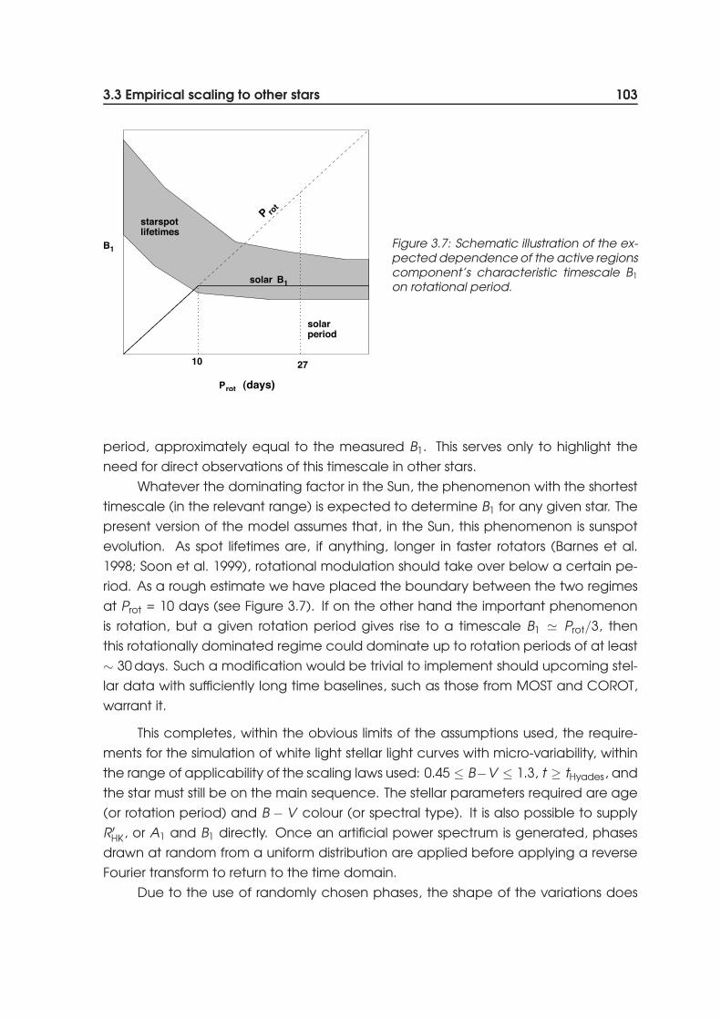
Figure 3.7: Schematic illustration of the ex-pected dependence of the active regionscomponent’s characteristic timescale B1

on rotational period.

period, approximately equal to the measured B1. This serves only to highlight the

need for direct observations of this timescale in other stars.

Whatever the dominating factor in the Sun, the phenomenon with the shortest

timescale (in the relevant range) is expected to determine B1 for any given star. The

present version of the model assumes that, in the Sun, this phenomenon is sunspot

evolution. As spot lifetimes are, if anything, longer in faster rotators (Barnes et al.

1998; Soon et al. 1999), rotational modulation should take over below a certain pe-

riod. As a rough estimate we have placed the boundary between the two regimes

at Prot = 10 days (see Figure 3.7). If on the other hand the important phenomenon

is rotation, but a given rotation period gives rise to a timescale B1 # Prot/3, then

this rotationally dominated regime could dominate up to rotation periods of at least

∼ 30 days. Such a modification would be trivial to implement should upcoming stel-

lar data with sufficiently long time baselines, such as those from MOST and COROT,

warrant it.

This completes, within the obvious limits of the assumptions used, the require-

ments for the simulation of white light stellar light curves with micro-variability, within

the range of applicability of the scaling laws used: 0.45 ≤ B−V ≤ 1.3, t ≥ tHyades, and

the star must still be on the main sequence. The stellar parameters required are age

(or rotation period) and B − V colour (or spectral type). It is also possible to supply

R ′HK, or A1 and B1 directly. Once an artificial power spectrum is generated, phases

drawn at random from a uniform distribution are applied before applying a reverse

Fourier transform to return to the time domain.

Due to the use of randomly chosen phases, the shape of the variations does


Figure 3.8: Comparison of a portion ofPMO6 data starting 1300 days after thestart of the full light curve (top panel)with a simulated light curve generatedusing the Sun’s observed rotation period(25.4 days) and chromospheric activity in-dex (R′

HK = −4.89, Radick et al. 1998). Bothlight curves have 15 min sampling, last180 days and are normalised to a meanflux of 1.0.

not closely resemble the observed solar variability. It may be possible to characterise

the sequence of phases characteristic of a given type of activity-related event, such

as the crossing of the stellar disk by a star-spot, faculae or active region. This infor-

mation could then conceivably be included, with appropriate scaling, in the model,

in order to make the shape of the variations more realistic. However, how to do this

in practice is not immediately obvious, and will be investigated in the future. As the

model stands, the simulated light curves can be used to estimate quantities such as

amplitude, timescale, the distribution of residuals from a mean level, but no conclu-

sions should be drawn from the shape of individual variations.

3.4 Testing the model

3.4.1 Mimicking the Sun

A first check is to compare the predicted observables for the Sun to the measured

values. The measured period and log⟨R ′

HK

⟩are 25.4 days and −4.89 (Radick et al.

1998), in good agreement with the predicted values of 23.4 days and −4.84. The

measured rmsby is # 5 in units of 10−4 mag. The value measured from a simulated

light curve with 1 day sampling lasting 6 months, when allowing for the conversion

between rmswhite and rmsby is 6.11. This slight over-prediction is attributable to the

Sun’s slightly slow rotation and low activity for its age and type, and to the fact that it

is slightly under-variable for its activity level (it falls slightly below the fit on Figure 3.6).

Figure 3.8 compares a portion of the PMO6 light curve taken from a relatively high

3.4 Testing the model 105

Figure 3.9: Examples of simulated light curves containing micro-variability for Hyades age(left column) and solar age (right column) stars with spectral types F5 (top row), G5 (middlerow) and K5 (bottom row). A single transit by a 0.5 RJup planet has been added to each lightcurve 75 days after the start (a transit by an Earth-sized planet would be ≈ 25 times smaller).The light curves have 1 hr sampling and last 150 days.

activity part of the solar cycle with a light curve simulated using the observed rota-

tion period and activity index of the Sun. The amplitude and typical timescales of

the variations are well matched.

3.4.2 Trends with age and mass

A set of six light curves have been simulated, corresponding to three spectral types

(F5, G5 and K5) and two ages (625 Myr and 4.5 Gyr). Examination of the light curves

and the various parameters computed during the modelling process can reveal any

immediate discrepancies. The light curves are shown in Figure 3.9 and the param-

eters in Table 3.2. They follow the expected trends, variability decreasing with age

and B − V and increasing with Prot, so that at solar age age the least active star is

the F star, while the most active is the K star, despite its long rotation period (due to

the dependence of activity on colour).


Table 3.2: Parameters of the simulated light curves.

Age SpT B − V Prot log(R′

HK

)A1 B1 rmswhite

Gyr days ×105 days ×104

0.625 F5 0.44 2.9 -4.64 19.27 2.89 22.00.625 G5 0.68 8.8 -4.44 38.16 8.80 46.50.625 K5 1.15 12.6 -4.42 41.40 9.84 69.5

4.5 F5 0.44 7.8 -5.23 4.66 7.87 13.34.5 G5 0.68 23.7 -4.80 11.95 9.84 13.94.5 K5 1.15 33.8 -4.67 17.53 9.84 14.4

3.4.3 Behaviour at high activity

Comparing the light curves shown in the left column of Figure 3.9 which have am-

plitudes of ∼ 0.5 %, to published V -band amplitude measurements for Hyades stars

(Messina et al. 2001, 2003), which are of the order of ∼ 3 %, immediately highlights a

discrepancy. This discrepancy could be explained by a number of factors:

3.4.3.1 Bandpass

Part of the difference is readily explained by the fact that the model produces white

light flux variations, while the amplitudes reported by Messina et al. were V -band

magnitude variations. As previously mentioned, white light flux variations in the Sun

are observed to be ≈ 2.78 times smaller that b & y magnitude variations, and a

similar effect is expected with V . To estimate the amplitude of such an effect requires

the comparison of simultaneous light curves in V and either b & y or white light.

S. Messina (priv. comm.) did this comparison and found near-identical variability

levels both in amplitude and in rms. The bandpass effect could therefore account

for no more than a factor of ∼ 2.8, which is not enough to explain the observed

discrepancy.

3.4.3.2 Underestimated rms values at high activity

As outlined in Section 3.3.1.3, the activity-variability relation remains ill-constrained at

high activity levels, with only one data point with[R ′

HK

]5

> 5.5. Although many stars

have been used to calibrate the relation over the range of activity levels typical

of the Hyades – 1.6 <[R ′

HK

]5

< 5 – there is a lot of scatter over that range and

different sources of data show different trends, indicating that systematics are still

present. However, given that the inclusion or exclusion of such “dubious” datasets in

the calibration hardly alters the scaling law, this is unlikely to be a significant factor.

3.4 Testing the model 107

3.4.3.3 Amplitudes versus rms

Simulated and observed light curves for the Sun were compared in Section 3.4.1, and

both rms values and amplitudes are consistent. For younger stars, the calibration of

the scaling law used should ensure that the rms of the simulated light curves approx-

imately agrees with observations (see previous paragraph). However, if the ampli-

tude scales differently from the rms as the activity level increases, the model could

produce sensible rms values but underestimate the amplitude for active stars. This

is possible if the statistical nature of the variability changes from relatively stochastic

(dominated by the emergence, evolution and disappearance of spots, as we think

is the case in the Sun) to close to sinusoidal (dominated by rotational modulation of

small numbers of large, persistent active regions, as is generally thought to be the

case in young active stars). In this case, a new component, more concentrated in

period space around the stellar rotation period, could be added to the simulated

power spectra.

3.4.3.4 WIRE time series data of α Centauri

The WIRE6 or Wide field InfraRed Explorer is a NASA satellite designed to perform sky

surveys in the IR, whose original goals could not be fulfilled due to loss of detector

coolant early in the mission. However, the rest of the satellite is in good condition and

its 5 cm aperture star-tracker telescope has been used successfully for asteroseismic

studies of a number of stars, including α Cen (Schou & Buzasi 2001). α Cen is a par-

ticularly interesting target to search for low-frequency variability such as is observed

in the Sun, as it is a well studied binary whose primary has a spectral type and age

close to that of the Sun. Recently, Kjeldsen et al. (1999) measured excess power in

ground-based radial velocity observations of it the range 600 to 3000 mHz, to which

they fit a powerlaw with a slope of −1.46, and which they interpret as granulation.

An attempt was made to use the WIRE time series, which lasts 50 days with ap-

proximately 40 % duty cycle (observations are taken during just under half of each

102 min orbit) to perform an analysis similar to that which was done for the solar

PMO6 data, fitting a multi-component broken powerlaw model to the power spec-

trum to obtain further constraints on the various parameters of our micro-variability

model. However, the complex window function could induce many features in the

power spectrum. To check for these, a Fisher randomisation test was carried out: a

‘scrambled’ dataset was constructed by drawing samples in random order from the

original dataset, keeping the same window function. There were no noticeable dif-

ferences between the power spectra of the scrambled and unscrambled datasets.

6http://www.ipac.caltech.edu/wire/


This implies that any features in the power spectrum of the unscrambled dataset are

in fact due to noise and the effects of the time sampling.

As α Cen was the WIRE target with the most complete light curve to date,

this suggests that little useful information relating to stellar micro-variability on the

timescales of interest for transit searches is likely to be extracted from WIRE data. The

first measurements of this type of variability in other stars than the Sun (excluding

active stars) are expected to become available in the near future thanks to the

MOST (Micro-variability and Oscillations of Stars) satellite.

3.5 Discussion

A model to generate artificial light curves containing intrinsic variability on timescales

from hours to weeks for stars between mid-F and late-K spectral type and older

than 0.625 Myr has been presented. This model relies on the observed correlation

between the weeks timescale power contained in total solar irradiance variations

as measured by VIRGO/PMO6 and the Ca II K-line index of chromospheric activ-

ity. Except for the most active cases, the resulting light curves appear consistent

with currently available data on variability levels in clusters and with solar data. Fur-

ther testing and fine-tuning requires high sampling, long duration space-based stellar

time-series photometry and will be carried out as such data become available.

The simulated light curves can be used to test the effectiveness of pre-transit

search variability filters (see Chapter 4) and to estimate the impact of micro-variability

on exo-planet search missions such as COROT, Eddington and Kepler (see Chap-

ters 5 and 6).

All the simulated light curves produced so far, as well as the routines used to

generate them, have been made available to the exo-planet community through

the web page: www.ast.cam.ac.uk/∼suz/simlc. Light curves with specific pa-

rameters can be generated on request. The model has been included in light curve

simulation tools developed for the COROT mission.

It is important to stress that the present approach, which is highly simplified

and empirically based (and which will be referred to hereafter as ‘the simulator’,

for clarity), differs from, but complements, more detailed theoretical models of the

complex physical mechanisms that give rise to the observed micro-variability of the

Sun (here after ‘detailed models’). There has been recent progress in the latter area:

for example, Seleznyov et al. (2003) successfully model the full power spectrum of

the VIRGO/PMO6 observations by combining the magnetic activity model of Krivova

et al. (2003) (which relies on identifying active regions in resolved solar disk images

and modelling their photometric signature) and a simple granulation model. Scaling

3.5 Discussion 109

this approach to other stars is non-trivial, but there will be much to learn from detailed

models about how the physical mechanisms at work vary from star to star when

upcoming high precision stellar photometric time series data become available. On

the other hand, our simulator has already been put to use to simulate light curves for

a wide range of spectral types and ages, thereby providing insights relevant to the

design of transit search missions and associated data analysis techniques. However,

its simplicity naturally limits its information content. Its applications rest more on the

statistical side: provided the overall trends are correct, it can be used, for example,

to place planetary transit detection limits for a given type of parent star.

Future improvements of the simulator will be two-fold. Of course, direct fitting

of the power spectra of other stars than the Sun, from MOST or COROT, will provide

direct constraints. In parallel, regions of parameter space not yet covered by these

missions can be explored using detailed theoretical models, to unveil the depen-

dence of the power spectrum on the parameters of the models. If the dependence

of those on stellar parameters is known, or if reasonable assumptions to that effect

can be made, the simulator can be adjusted to reproduce similar trends in the power

spectra it generates.

Another step currently under consideration is the extension of the simulator

to produce light curves in specific spectral band passes. This would be very use-

ful in the context of COROT (and potentially Eddington) whose design includes the

use of colour information, both for target selection and the preparation of colour-

discriminant light curve analysis tools.

c h a ra c te risin g a n d sim u la tin g ste lla r m ic ... · tu d e o f th e va ria tio n s c a...

Documents