HAL Id: jpa-00222553https://hal.archives-ouvertes.fr/jpa-00222553

Submitted on 1 Jan 1983

HAL is a multi-disciplinary open accessarchive for the deposit and dissemination of sci-entific research documents, whether they are pub-lished or not. The documents may come fromteaching and research institutions in France orabroad, or from public or private research centers.

L’archive ouverte pluridisciplinaire HAL, estdestinée au dépôt et à la diffusion de documentsscientifiques de niveau recherche, publiés ou non,émanant des établissements d’enseignement et derecherche français ou étrangers, des laboratoirespublics ou privés.

STORIES OF UNDULATOR LIGHTC. Elliott

To cite this version:C. Elliott. STORIES OF UNDULATOR LIGHT. Journal de Physique Colloques, 1983, 44 (C1),pp.C1-255-C1-287. <10.1051/jphyscol:1983124>. <jpa-00222553>

JOURNAL DE PHYSIQUE

Colloque Cl, supplément au n°2, Tome 44, février 1983 page Cl-255

STORIES OF UNDULATOR LIGHT

C.J. E l l i o t t

Los Alamos National Laboratory, Los Alamos, lieu Mexico 87546, U.S.A.

Résumé.- Nous passons en revue les travaux effectués sur les lasers à électrons libres incluant : un exposé des principales idées destiné aux profanes; un récit historique des travaux accomplis au cours de ces dernières années; une caractérisation mathémati­que de divers projets; une formulation du problême mathématique comme problème non linéaire à point fixe; une description des techniques de calcul.

Abstract. - We review optical details of free-electron lasers including: a layman's account of many of the ideas; a historical account of work over the last two years; a mathematical characterization of various schemes; a formulation of the mathematical problem as a non-linear fixed-point problem; and a description of computational techniques.

A. Introduction.

The purpose of this paper is to summarize and categorize work which has

occurred over the last two years that treats the optical details of the Compton

regime free-electron laser (FEL). These details are important in assessments of

optical quality and optical-resonator design. By the term optical details I mean

the description of the dependence of the optical field on coordinates transverse to

the axis of the optical resonator. Virtually no discussion is given here on the

longitudinal dependence of the field (the pulse train structure).

The audience at which this paper is directed is primarily those who are

contemplating undertaking or utilizing such calculations, but this review is also

useful for those who simply want to know what is occurring in the field. Section B

should be understandable to a non—technical person who is interested in an overview

of the ideas as opposed to the implementation of them.

The remainder of this section gives a brief description of the parts of this

paper, and then it goes on to define the problem and concepts used. Section B

serves to translate the major ideas into non-technical terms; it can be skipped by

those well versed in the field. Section C reviews work on various physical models;

it starts with oversimplified models (the classic models) and goes on to describe

the work of the last two years (the 1981-1982 models) and finally gives a preview of

work to come. Section D examines these models from the point of view of the

underlying mathematical ideas; this section starts with a description of the flow of

Article published online by EDP Sciences and available at http://dx.doi.org/10.1051/jphyscol:1983124

Cl-256 JOURNAL DE PHYSIQUE

ideas from Maxwell's equations to the actual computations; it then abstracts a

general non-linear description that allows the various techniques to be categorized

and points to new techniques; finally it points out that optical propagation in

cavities can be formulated as a non-linear fixed-point problem. Section E delves

into the digital operations necessary to carry out computations of optical beam

quality; it starts by looking at available computer power, and then it goes on to

describe ghost cell requirements that occur in finite grid techniques; finally it

looks at the various methods of handling the optical part of the problem and

concludes that the choice should often be based on convenience as opposed to

efficiency of the algorithm.

Mathematics is a language that enables us to state precisely what problem we

are addressing. We start with the vector potential,!, and the transverse driving

current J1 that is produced in the interaction region by interplay between the

radiation field, the static magnetic field, and the relativistic electron beam. The

wave equation, in the radiation gauge, is

2 1 a!? v2A - - =

- c2 at2 -'JoJ1

and is subject to reflecting boundary conditions at the mirrors, and radiative

boundary conditions,transversely, at infinity. The well studied empty cavity modes

are the solutions, for JL = 0 , to the eigenvalue problem that requires the optical

field on one mirror to be a complex-number multiple (the eigenvalue) of that same

field after it has propagated a round trip in the cavity. The loaded cavity mode is

the solution for finite JJ. The transverse current, .JI, can itself be thought of as

radiating into a superposition of the empty-cavity modes, and it is the feedback

enhancement of these empty cavity modes that determines their contribution to the

loaded-cavity mode.

It is only in low gain devices that empty-cavity modes form a good basis for

describing the loaded-cavity problem. (Note one often has strong signal even though

the gain per pass is low.) When the gain is high and the device is long, non-linear

effects similar to self-focusing can overcome diffractive spreading of the optical

beam and entrain the optical pulse in the electron beam. In these cases the

electron dynamics, that lead to lensing, and the optical propagation are tightly

coupled together.

In describing optical quality from an optics point of view, we can think in

terms of the index of refraction and the absorption or gain. Both the gain and the

index of refraction may be thought of as complex quantities and the relationship

between them is given here. Suppose we have a complex gain coefficient, gc. Then

we expect a free-space plane wave having z dependence, exp[i(w/c)z], to be modified

by the multiplicative factor, exp(gcz). The modified wave can be described by a

complex index of refraction,nc, where

Another convention is to use

or equivalently,

where Re and Im are the signed lengths of the real and imaginary parts respectively.

Although neither the complex conductivity nor the complex dielectric constant have

appeared in the literature on the optical quality of FELs, they too are simply

related concepts and might be preferred in future publications.

In the case of a low gain FEL, to understand the possibility of good optical

beam quality, it is useful to think in terms of the incident field, E (the incident field that we often think of in of an oscillator is that at the design point), and

the excited field k . If we look at the field far away from the interaction region

(ignoring the mirrors) the energy density is proportional to l + ~ 1 ' . With low gain,

the radiated intensity increment is the cross term 24*E, and if we think of the FEL

interaction region as a single entity this term is the (in-phase) stimulated

emission. The spatial dependence of this intensity-increment cross term is the

product of the spatial dependences of the excited wave and the incident wave. Thus,

even though the excited wave may radiate over a large spatial region, the intensity

increment associated with the stimulated emission may be found over a smaller region

because the incident wave is nearly a cavity mode whose far-field dimensions may be

considerably smaller than the excited wave.

Cl-258 JOURNAL DE PHYSIQUE

The procedures for attacking the problem of describing the FEL optical details

are many. There are also a great variety of tastes as to the physical description.

The particle motion is described elsewhere, the starting point being a Lorentz force

equation, or a relativistic Hamiltonian. The starting point for optical details is

Maxwell's equations. These details are complicated enough without including the

time-dependent pulse structures; i.e. only one fourier component of the field is

studied. In these single frequency pulse cases all methods that have evolved are,

in principle, equivalent to each other and to the paraxial-wave-equation description

(see Section D). Of course, the numerical implementations which are the steps in

going from the paraxial wave equation to a discrete calculation differ according to

the representational grid and the propagation methods.

One final comment on terminology comes from David Deacon. In the United States

the term wiggler has often been used to describe the static magnetic field of the

free-electron laser interaction region. In Europe wiggler often has an additional

restriction: it is applied only to magnetic fields that are weak. To avoid

confusion we do not distinguish between strong and weak fields and refer only to

undulators.

B. Happenings Of Light In Servicing The Interaction Chamber: A Holistic Approach.

\ r e f ~ e c t i n ' ~ surfoce reflecting surface interact ion

chamber

Fig.1 - The optical wave bounces back and forth between the pair of reflecting mirrors. The wave of undulator light is produced originally by fast electrons that are pushed and pulled (wiggled) by the static magnetic field, the undulator. The fast electrons come from an accelerator that has increased the electrons' mass many fold above their rest mass. These electrons arrive in bursts that are separated by the time it takes light to make a round trip. The undulator light they produce, the excited wave, gets added to the incident wave to form the sum wave that gets reflected in the mirrors and becomes the new incident wave. The intensity of the undulator light grows until the burst of electrons can only give it the small fraction of its energy lost on reflection.

The device we call an EEL is shown in Eig.1. The excitation of the optical

wave begins slowly as the interaction begins, and gradually over-massed electrons

become trapped by the interplay of the optical wave and the static magnetic field

that wiggles the electrons back and forth in transverse fashion. These electrons

become excited and give off light. This process of stimulated emission is a source

of energy to the optical wave and causes the electrons to lose energy and reduce

their speed in accordance with the laws of Nature. This energy comes by way of the

excited wave that has taken the time and energy of electrons to help create. The

time it takes the electrons delays the peak intensity of the excited optical wave

and the resultant optical wave is then characterized by lethargy, a term that also

describes the enervated motion of the electrons that are still significantly

over-massed. Various schemes to enable the electrons to give more of their mass per

pass and to recover left-over energy of the electrons as they are brought to the

rest-mass condition are actively under experimental study.

The mathematical model has an intrinsic beauty when couched in the terms of the

powerful wave equation driven by well known Lorentz-gauge electron currents. The

waves that occur are of two types: permanent (or static) fields and naturally free

(or propagating) fields. The naturally-free fields that propagate in the EEL are

refered to as optical (light) waves and these are of two types. The incident

optical wave is curl-free everywhere, and the excited optical wave has a non-zero

curl as it is produced in the interaction chamber, but the excited wave loses its

curl when abandoned by the electrons. Upon summation to the incident wave and after

losing a little energy upon further reflection in several mirrors, it may be

regarded as the new-incident wave, more energetic than the last and ready for a go

around with another group of electrons that are well prepared to enter the

interaction chamber. Where does this lead you may ask? It is almost like a fairy

tale in which the wicked witch is punished by seven years of bad luck. Things are

not that grim; as the incident wave becomes more and more powerful it soon

aggregates much more energy than any single group of electrons can give it; it

eventually stops growing when the relatively small amount of energy lost in

reflection becomes as large as the amount supplied by the electrons.

You may wonder if after this explosive growth of the incident wave, whether it

is capable of settling down to a predictable stable existence or will it lose and

gain randomly, sometimes on the left side, sometimes on the right side, sometimes

here, and sometimes there? You will see that as the story unfolds it all depends on

the group of electrons with which the incident wave interacts. It also depends on

how the incident wave began in the dark. There are some unusual incident waves that

can interact with a number of electrons so large that it would drive most waves

chaotic. These have been named the strange attractors, and they exist on the

islands of stability, changing character as they roam the island but always staying

there. Between these isles the sea of chaos reigns. If even more electrons are

used in a particular reduced mathematical description, intended for electrons that

C 1-260 JOURNAL DE PIIYSIQUE

do not influence each other's motion, there comes a point where the domains of the

strange attractors no longer exist. This space of incident waves is completely

covered by a turbulent sea of chaos. Here the incident waves come and go in

unpredictable fashion. They might remind you of a strange attractor you had

previously encountered and then on the next pass they may resemble a completely

different strange attractor. Yet with enough electrons the behavior is completely

aperiodic and utterly wild.

The realm of fancy possibility is truly mind boggling, so we will describe the

more predictable aspects of the theory where the incident wave settles down to a

fixed shape. In describing these cases the entire space of wave functions is much

too extensive for our purposes. We are interested primarily in those optical waves

traveling through the interaction chamber in nearly the same direction as the

electrons. It is these waves that can grow at the expense of the electrons. The

interaction chamber can be thought of, for Platonic simplicity, as a narrow tube

that is long but finite in the direction the electrons are traveling. The chamber

is regarded as narrow because the electron beam is narrow; the chamber is an

artificial delimitation of space telling us where the over-massed electrons are

located when they interact with the optical fields. We can imagine many types of

electron beams: some fill the cylindrical chamber uniformly in the narrow

(tranverse) direction, some have more electrons at the center of the chamber, others

might be contained by a rectangular cylinder. Of course, all of these chambers are

invisible to the optical waves because the chambers are simply figments of our

imagination. Another aspect of the class of problems we address is that the mirrors

for the optical waves are at either end of the interaction chamber. If the optical

wave leaves through the narrow dimensions of the interaction chamber, we do not

allow it to reenter; we give it only one chance in the interaction chamber per pass.

By placing these restrictions, some progress can be made on a reduced mathematical

description, but even this problem is more difficult than that currently attempted.

The mathematical idealizations that have been attempted so far do not describe

actual physical situations, but rather they extract a subset of features of the

physical problem that they describe faithfully. The remainder of the features are

described in a distorted fashion that may even be unnatural in the physical world.

An analogy might be the study of the flight of an airplane by means of a physical

model of only the wings. Clearly a restricted set of questions may be asked of this

model problem; e.g., questions of lift are expected to be reasonably described;

questions of tire wear are not addressed; and questions relating to drag are only

partially answered.

The questions we may ask involve nouns and verbs. We have already become

acquainted with the elements of the FEZ. problem: the electrons, the incident wave,

the excited wave, and the permanent field. Each of these elements have attributes

that may be described by nouns such as the length and breadth of each of the

elements. It is the wave equation that tells us which nouns are important. It

relates how each of the waves vary in space and time at a particular point and time,

with the electron-current value. The electron current depends on the instantaneous

position, speed, and direction of all the electrons in the immediate vicinity of the

point under examination in the wave equation. Given an initial description of the

nouns, the wave equation describes what happens.

The nouns that appear in the wave equation are the electron current and

derivatives of the gradients in the size of the optical fields in each of three

directions, whereas the verb is the rate of change in the field with time. Given

the nouns that describe the element of the problem, the wave equation provides the

verbs. The wave equation may be thought of as the weaver of stories about how

optical pulses behave in the presence of electron currents, and it has many tales to

tell.

Not only must we pay attention to the wave equation story teller, we must also

simultaneously listen to other tales that are woven by the particle equations of

motion. For the class of problems we are describing, the electrons do not alter

each others motion significantly, but rather move according to the single permanent

magnetic field and the propagating fields in which they are immersed. Our situation

is somewhat like watching an opera where the stories of all the characters

(electrons) are evolving simultaneously as the orchestra plays the music (incident

optical field), and the characters add their own arias (excited optical field)

hopefully in harmony with the orchestra. But rather than the situation in most

musical operas where the characters influence each other strongly, in our optical

opera the characters (electrons) react only to the musical ambiance (the optical

waves) of the moment, and disregard what the other electrons are doing except

through their emitted waves (arias). In most of the work we will describe, the

incident wave (orchestra) dominates over the excited wave (that was emitted by the

electrons). An exception is the work of Prosnitz, Doss, Haas, and Gelinas [I] where

the incident wave (orchestra) starts the process off and then is soon out done by

the excited wave; at that time the orchestra (incident wave) simply cannot be heard

and might as well stop playing. The opera analogy describes the type of interaction

between the waves and particles, but it fails to describe the spatial distribution

and motion of the waves and particles.

The stories of the wave equation that I have selected to tell you have several

things in common. First they all start out in a similar fashion with the incident

optical wave entering the interaction chamber from the left, apparently in a hurry

with a speed called c. The electrons also enter from the left, simultaneously with

the wave, traveling almost as fast. Although the electrons had been pushed a great

deal, the faster they went the more mass they obtained, and the more mass they'had,

the harder it was to make them go faster; such was their lot: if they started out up

front on the wave soon they would slip toward its rear.

C1-262 JOURNAL DE PHYSIQUE

This slippage along with careful timing is the key to successful EEL action by

electrons that do work on (for) the optical field. The electron's work depends on

the electrons being able to move in a direction opposite to that of the optical

field. Their motion depends on the presence of the static wave, the magnetic field,

that perturbs the electrons and sets them in a spin or causes them to totter as if

inebriated. Ideal timing by the most efficient electron occurs if that electron

totters to the left when the optical field is pointed to the right and is at her

peak positive value. Then at the moment the electron has slipped back toward the

rear of the optical wave where the wave is most negative and is pointed to the left,

our efficient electron is tottering to the right, always opposing the field.

Electrons that do work lose energy and slow down so that they slip at an even

greater rate toward the rear of the optical wave. The rate of electron energy loss

depends on where the electrons are in the interaction region. As they progress

through the interaction region, the static magnetic field is designed to cause the

electrons to totter back and forth even faster to compensate for the increased rate

at which the optical wave changes its sign from the greater slippage rate. These

magnetic fields are called tappered because they gradually change their period to

accommodate to the reduction of speed of the efficient electrons.

The other common aspect of the stories is an almost timeless quality. The

stories we describe are actually not those of the wave equation itself. We employ a

model that makes the story repetitious and permits the optical wave to have only a

single color (monochromatic). Our model is simpler than the,actual storyteller

(wave equation), and it is a matter of speculation whether the model will ever be

close to the seasoned teller, that is, will the full wave equation exhibit solutions

that the simple model can describe in most of their important details?

We don't place sole blame on our apprentice (model) storyteller of the wave

equation for possible inconsistencies because the electron storyteller is not

genuine either. The story of the electrons also repeats itself after the same short

interval, and who is to say whether a periodic set of electrons drove the optical

wave periodic or vice versa. As suggested above it is not clear that the true

raconteurs could ever have gotten into this recurrent mess. Either the model for

the wave equation or the tyro particle teller said to the other, "If you will do it

again, I will too." And since it was a lot easier to do so, they went off and did

it, forgetting the boundary conditions specified by law. The legal problem is that

a consequence of this cabal led to an infinitely long pulse and an infinite amount

of energy. Now it can be argued that perhaps a very long pulse of finite energy

will not vary in peak amplitude (i.e. it would be monochromatic or periodic)

halfway through, but that raises start-up and shut-down questions. A partial

reassurance to assuage our annoyance is that physicists do not regard similar

transgressions in scattering theory as serious, although there the situation does

not involve as many interesting beams. When physicists discuss the infinite, it is

a most difficult topic.

Several of the stories continue, as we recounted earlier, with reflections in

the mirrors. We might like to think of these as additional stories about thin

slices, one optical period long, taken from very long beams that travel nearly

forwards (or upon reflection sometimes backwards). The electron beam can be

described as a thin slice of the interaction chamber crossection; it moves from the

beginning of the chamber to the end at the speed of light, slightly faster than the

electrons within. The electrons that slip out the back end are replaced by

electrons with identical transverse location, speed and direction of travel, at the

front end of the slice, so our repetitious story teller says. (There are other

important details of the electron motion we don't have time to recount.) Similarly

the optical slice is one wavelength long, with speed c, but because the substitute

story teller insists on a monotone, the description of the optical waves in the

optical slice is considerably simpler than the description of the electrons in the

spatially coincident electron slice.

The incident wave is sinusoidal as shown in Fig.2. In this three dimensional

representation, the height represents the amplitude of the wave, left to right

represents the propagation direction, and back into the plane of the figure and out

Fig.2 - A single period of a Gaussian optical beam. Left to right is the propagation direction. Away and towards us represents the radial distance from the center line of the optical system; r-0 occurs halfway back. The height is the amplitude of the optical field. If we look along the edge of a single stripe, the up and down motion we see is sinusoidal. The peak height on stripes occurs further to the right (are advanced) as we move out from the center plane and this indicates that the focal point is to the right.

C1-264 JOURNAL DE PHYSIQUE

of the plane represent a transverse dimension. As we look into and out of this

plane at the similar parts of the wave, they appear to be more advanced the further

we go away from the center plane (the center plane has directions of up and down and

left to right) of the wave. Also as the incident wave propagates it moves forward

or backward in the slice, but still keeps its overall sinusoidal shape in the

direction (axial) of propagation. By this, I mean that at the same transverse

position (as we slide along a stripe) the wave goes up and down in the same way it

does at another transverse position, except for possible shifts or delays. The only

data we need to know to describe the information of this wave everywhere in the cell

(slice) is the height to which it rises (as we slide along a stripe) and its

retardation (an advance is negative retardation); these quantities are also known as

the amplitude and phase of the wave. We now shift from the context of the space of

Fig.2 where height is the amplitude of the wave to a space where the height is the

other transverse direction of real space. The retardation or phase is measured by

the distance from a fixed transverse reference plane in the cell such as the length

from the end plane (containing the ridge at the right) of the slice to the location

of the peak of the wave. From each point (transverse location) on the reference

plane there will be a different measurement of the height and retardation or delay,

and we may think of these quantities as being stored on this transverse plane, two

values for each point. We could imagine a chess board as the transverse plane and

in each square two numbers one for the height and one for the delay would be written

at the center of the square. We might want to subdivide the squares finer and write

smaller so we could get a better description of the wave. In a computer, the chess

board numbers may be stored, two numbers for each square, and given a big enough

memory you may make the squares as fine as you wish.

The excited wave when added to the incident wave is known as the sum wave.

Both the sum wave and the excited wave are sinusoidal but have heights and

retardations that are usually different from the incident wave. We can either think

of there being two separate waves, the excited wave and the incident wave, or we can

think of just one, the sum. For some problems, one of these two representations is

more convenient. To obtain the sum height at a point in the cell we take the sum of

the two separate heights at that point and then we repeat the process for every

point in the cell. It is a matter of simple trigonometry to show that the sum of

two shifted sinusoidal waves with different amplitudes give another sinusoidal wave,

whose amplitude and retardation are algebraically related to those of waves added.

In the chess board description, this same algebraic formula could be used to do the

height and retardation representation of the sum. How and under what conditions the

excited wave generated by the electrons is actually sinusoidal is a story to be told

another time.

The full numerical description of the electrons requires more than one

chessboard, it requires many chessboards discretely placed at various axial

locations or phases as in three dimensional chess (or the Inner Circle game).

Coders have used between 30 and 500 stacked chessboards for special over-simplified

calculations in which the chessboard has only one square, and computations for

many-square chess boards are now in their infancy. By counting the many chess

boards, we can see that the description of the electrons is considerably more

involved than the single board description of the optical waves. A simplified model

for the electrons reduces the computation time considerably by requiring only two

numbers (rather than many pairs) on each square. One of the numbers on a chess

board square is the phase of the electron and the other is its energy (or mass or

alternately momentum). Another oversimplification is the selection of one chess

board, the resonant-phase board, to represent many electron chessboards. The less

efficient electrons on this chess board slip at a slower rate than the more

efficient ones. As the chess board for the electrons moves through the chamber,

each square has a different slippage so that the chess board disassembles into 64

(or more) separate squares, but since we have written the phase on the square, we

may think of the chess board as being reassembled and the axial position (phase) at

which each square would be located as being coded information stored on the

individual squares, should anyone ever want to actually see the real disassembled

locations.

In this resonant phase model the numerical calculation can be viewed as a two

board game. If the outcome depends on who (the electrons or the incident wave) goes

first then the game does not correspond to the physical problem. We want to take

small enough axial steps so we will describe the problem smoothly. The situation is

similar to film making where LO frames per second results in jerky motions, and 24

frames per second appears natural. For large steps the motions appear jerky, with

small enough steps we describe small changes in the motion and very little happens

in one step, so it makes little difference who starts. Although the picture of the

electrons and the sum wave alternately taking a turn (small step) is somewhat over

simplified, it contain the idea of how the story is told.

When the electrons move, they move according rules that depend on the sum-wave

chess board, and when the sum wave moves the rules depend on the electron board. It

might seem this game would be considerably harder than chess, but that is not so.

We are not taxing the power of present day computer in playing this two board game

(or even the many board game). We are not using game theory to guide the plays. It

is essentially different than chess in that there is no freedom of choice in the

moves: our story is automatically woven. Who would believe electrons had free

choice in the free electron laser? For our classical calculations God does not play

dice, but we wonder if there will ever be a Solon or Moses for electrons, or will

the stories remain just so.

JOURNAL DE PHYSIQUE

C. History of the Models.

This section summarizes work done on transverse optical-detail models for FELs

utilizing large-mass (relativistic) electrons. Here a description of what work has

been done is given without emphasis on conclusions or speculations. Much of the

language used is aimed at those who have had a good grounding in classical

electrodynamics [2] and who are familiar with the variable-parameter FEL

calculations [3] that do not describe transverse optical details. If you get bogged

down, going to the sources will be helpful.

1. The Classic Models.

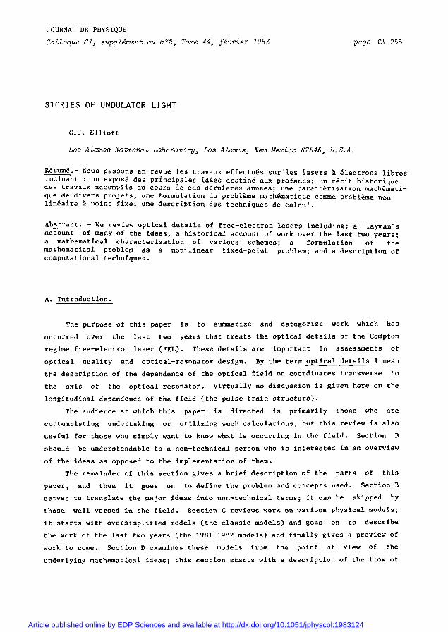
We may obtain a fuzzy picture, see Fig.3, of how the optical wave travels

through the interaction chamber by balancing the loss of energy to the electrons

with a gain in the optical energy and by introducing a filling factor. We think of

this optical wave as being flat (a plane wave). After moving the electrons a small

step through the interaction region and computing the average energy lost by the

electrons, we may compute the total energy lost from all electrons with

multiplication by the total number of electrons. Then the volume of the optical

pulse together with the energy density (energy per unit volume) of the incident wave

permits us to compute the energy density of the new-incident wave. If we think of

the electron number density as being fixed, it follows that the total energy lost by

the electrons is proportional to the size of the volume containing the electrons.

Because this source of optical energy is fixed, the increase in optical energy

density varies inversely with the optical volume. Thus, the optical energy denpity

increment is proportional to the electron-beam volume and inversely proportional to

the optical-beam volume. The ratio of these two volumes is known as the filling

/ electron volume

pt ical ol u me

Fig.3 - The energy balance model takes the filling factor to be the ratio of the electron volume to the optical volume.

factor, one number that in the theory replaces two numbers, the separate volumes of

the beams, and the filling factor is the only geometrical concept in this simple

model.

The above energy balance technique is elementary but incomplete; it leaves many

questions about the evolution of the optical pulse unanswered by providing only one

piece of information. Is it as if we have applied a projection operator to the wave

equation that permits it to ask only one question in question space? (See Fig.4.) In

satisfying this one question, it is clear that other dimensions of the description

are missing: e.g., how is the energy distributed? Do we keep the same energy per

unit volume and use a larger volume, or do we keep the volume the same and increase

the energy density? Do we concentrate the energy in globs or do we distribute it

uniformly?

To project answers to these other questions more information needs to be

extracted from the wave equation. Better physical pictures are achieved by more and

more elaborate models that answer more and more questions. Beyond the energy

balance approach comes a geometric optics treatment. By use of rays parallel to the

center axis of the interaction region (going left to right), we may arrive at a

filling factor description that also gives us the phase retardation of the optical

wave. By use of Wigner distributions or other means that incorporate non-parallel

rays we can describe optical beams that shrink and grow (and mock diffraction) as

they pass through the chamber. With this approach the concept of the filling factor

can be defined at the center of the chamber where we expect the optical volume to be

nearly minimum (and the optical energy density, a maximum). Alternately, an average

filling factor could be defined.

,,...THIS POINT IS THE ' E N E M BALANCE

QUESTION.

Fig.4 - Question space showing energy balance as a central question in one portion of the space.

Cl-268 JOURNAL DE PHYSIQUE

The optical cavity can be modeled as a device that takes the sum wave, projects

out a lowest order Gaussian mode, and multiplies that @art by a reflection

coefficient. This suggests a model in which the excited wave is replaced by that

part of the excited wave radiated into the fundamental Gaussian mode, or

equivalently, by producing an operator that projects out that portion of the

electron current radiating into such a mode. This approach can be handled in the

context of the paraxial wave equation and is similar to work published by Moore and

Scully (MS) [4] in 1980, more recent work of Colson and Elleaume [5], and work

reported at Santa Barbara in March 1982 by Tang and Sprangle.

2. The 1981 - 1982 Models. The rest of the work described here brings us up to date with the next level of

abstraction that uses the paraxial wave equation to treat non-Gaussian, transverse

variations. These treatments do not remove the monochromatic (periodic) requirement

nor do they treat many slices of time. They do, however, use realistic boundary

conditions at the mirrors, for oscillator (cavity) problems. Questions involving

the impact of lethargy or the effects from electrons slipping a substantial portion

of the optical beam on optical beam quality are ignored.

The focus is on solving the paraxial wave equation by digital calculations on

computers. Although similar work has been done for conventional laser systems, not

everyone interested in this level of detail is familiar with that work. Prior

methods of solving the partial differential equation, the paraxial wave equation,

feature finite differentials 16-81, Gauss-Laguerre polynomials [9,10], Gauss-Hermite

polynomials [10,11], Fresnel-Kirchhoff integration [12], quasi-fast Hankel transform

(QFHT) [13-151, and fast fourier transform (FFT)[16-181. In application to our

laser, all of these methods incorporate production of the excited wave with

distribution by carrier transport in a left-to-right or right-to-left fashion, much

like an automobile carrier transporting newly made sedans on a freeway.

The latest innovations in electron engineering in these models include tapered

magnetic (mag.) fields and bucket traps designed for a single electron.

Discriminating consumers who are looking for a vehicle to transport a family of

electrons will have to wait because these models are still in the test stage.

A prior innovation by Sprangle and Tang (ST) [19,20], in which they sacrificed

no generality, resulted in an integral Lagrangian formalism. Although this model

was highly original, its deployment required knowledge of the entire futures of

electron families, futures that depended on the predictions of the model. For

specialized uses where the excited wave had little impact on the electrons, and

where the electrons followed a known Gaussian with a fixed radial width, the ST

model predicted lensing effects that distorted the appearance of the (sum) optical

wave. These effects were also pointed out by others [3]. Although the ST model

crammed all the electrons into the bucket trap, rather than just those that would

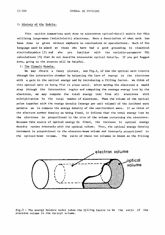
have been caught with an adibatic model, results (see Fig.5) stirred the

imaginations of the designers who have worked with the 81-82 models.

cos yR=0.6 f PHASE (rad)

Fig.5 - Phase of a Gaussian electron source of excited waves at various distances from the beginning of the interaction region. The phase may be thought of as a retardation of the wave in time or space.

The inherent difficulties of the ST model were sidestepped by Slater, Lowenthal

and Quimby (SLQ) [21] who turned to a partial differential approach with finite grid

implementation late in 1980. This transverse grid effectively traveled back and

forth through the interaction region and reflected from the mirrors until a steady

state successfully ensued. It enables evaluation of tradeoffs due to inability to

match the optical field to the magnetic field at all radii. SLQ also reported a

comprehensive design of the FEL chamber that included tradeoffs between optical beam

quality, magnetic field strength, and magnetic field inhomogenities. On the one

hand the magnetic field strength was to be made as intense as possible, by

decreasing the separation between permanent magnets, but on the other hand an

aperture that is too small will destroy optical beam quality and gives unacceptably

large transverse variations of the magnetic field in the interaction chamber.

Figure 6 shows a map of optimum optical beam size and electron beam radius for

various interaction chamber lengths for 10 pm wavelength light (The optimum optical

beam size decreases for shorter wavelengths.)

Additional work by Quimby and Slater(QS) in 1982 [22] included graphical

presentation of their results in a cleafly written paper that was a delight to read.

They utilize a criterion that requires taking an electron out of its bucket for good

(detrapping without retrapping) when its contribution falls off due to too much

resonant phase shift. They also use many radial lanes (grid points) and describe

the effect of the magnet aperturing that produces the sharp protuberances shown in

JOURNAL DE PHYSIQUE

PHOTON BEAM

- E " - "l - n w

100

WIGGLER LENGTH ( m )

~ig.6 - Design map of electron-beam radius and optical-beam radius at the waist (minimum) and end (maximum) for lOpm light.

Fig.7 - Calculations of Quimby and Slater showing pulse intensity as a function of radius and axial location.

Fig.7. These self-consistent calculation use apodized mirrors to remove numerical

instabilities.

The SLQ results were a stimulus that led ' Elliott [ 2 3 ] to undertake a mode

expansion along the lines suggested by MS, but where the resonator modes in the

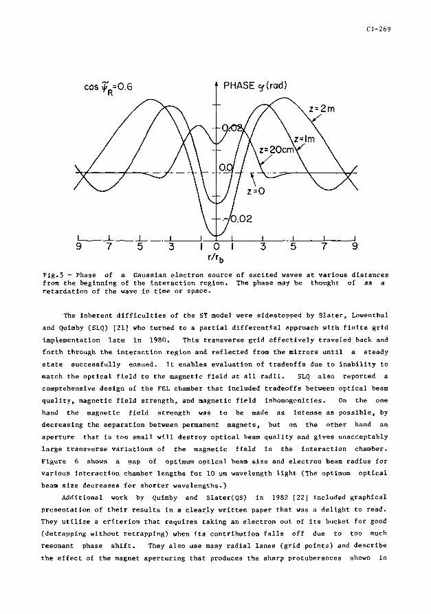
formalism are chosen to satisfy sharp-edged mirror boundary conditions. Cavity

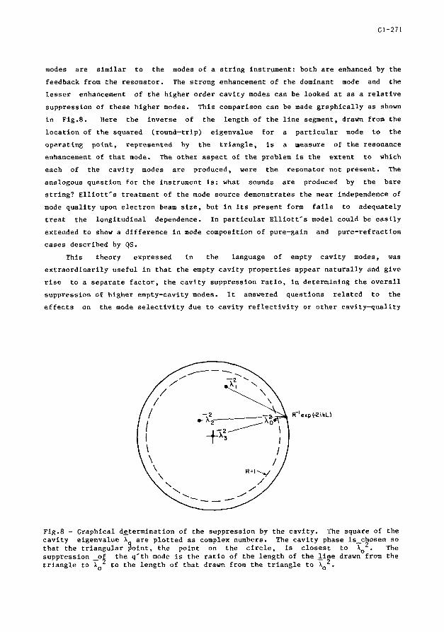
modes are similar to the modes of a string instrument: both are enhanced by the

feedback from the resonator. The strong enhancement of the dominant mode and the

lesser enhancement of the higher order cavity modes can be looked at as a relative

suppression of these higher modes. This comparison can be made graphically as shown

in Fig.8. Here the inverse of the length of the line segment, drawn from the

location of the squared (round-trip) eigenvalue for a particular mode to the

operating point, represented by the triangle, is a measure of the resonance

enhancement of that mode. The other aspect of the problem is the extent to which

each of the cavity modes are produced, were the resonator not present. The

analogous question for the instrument is: what sounds are produced by the bare

string? Elliott's treatment of the mode source demonstrates the near independence of

mode quality upon electron beam size, but in its present form fails to adequately

treat the longitudinal dependence. In particular Elliott's model could be easily

extended to show a difference in mode composition of pure-gain and pure-refraction

cases described by QS.

This theory expressed in the language of empty cavity modes, was

extraordinarily useful in that the empty cavity properties appear naturally and give

rise to a separate factor, the cavity suppression ratio, in determining the overall

suppression of higher empty-cavity modes. It answered questions related to the

effects on the mode selectivity due to cavity reflectivity or other cavity-quality

Fig.8 - Graphical determination of the suppression by the cavity. The square of the cavity eigenvalue A are plotted as complex numbers. The cavity phase is-chosen so that the triangular ftoint, the point on the circle, is closest to A~'. The suppression -of the q'th mode is the ratio of the length of the line drawn from the triangle to Ao2 to the length of that drawn from the triangle to .lo2.

factors. It also pointed to a new method of mode selectivity when modes have

different phase shifts from the dominant mode, even though these modes may have

little loss to begin with. It also appears to be the only work so far that has

checked to see that empty cavity properties are in agreement with published values,

and it extends the number of reported eigenvalues and should be a useful source for

checking other codes. This work also confirms and extends SLQ results that good

optical beam quality is achievable.

Prosnitz, Hass, Doss, and Gelinas (PHDG) [ l ] carried out work conceptually

similar to SLQ, but in an amplifier configuration (rather than an optical

resonator). They assessed the ability of effects similar to self-focussing to

overcome diffraction and to confine the optical beam to small radii over long

pathlengths and large gains. Rather than select a single electron in each bucket,

they use an average electron whose behavior represents a composite behavior of all

electrons. They also describe special problems that test their code for its optical

propagation and its ability to reproduce the electron description calculated in the

absence of diffraction.

PHDG describe two calculations for a proposed amplifier. The first calculation

matches the optical field to the magnetic field on axis and results in premature

focussing on axis. The second calculation matches the fields off axis at the

estimated radius of synchronism and shows that detrimental focusing can be avoided,

see Fig.9. The sensitivity of the performance of this device to the design-radius

parameter raises questions of how reproducible these results will be due to

shot-to-shot variations in the electron beam under actual experimental conditions.

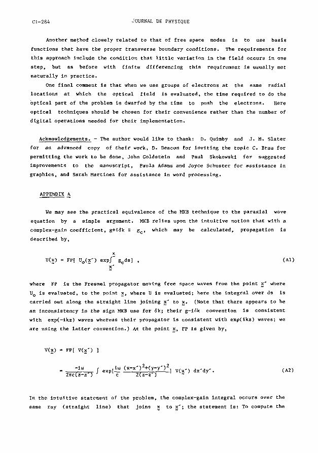
Mani, Korf, and Blimmel (MKB) 1241 attacked the loaded cavity problem in a new

way. They started with the Fresnel-Kirchhoff integral method concocted by Fox and

Li (121; to this they added descriptions of gain and phase that served the role of

the wave equation sources. This procedure may be bitter for new initiates; I myself

acquired a taste for it only after finding out that indeed the wave equation (story

teller) was satisfied with this particular mix (Appendix A). In their first

attempts at putting the theory together MKB did not follow their own prescription:

t'wit, they skimped on the ingredients but still obtained a whole, natural product

as seen in Fig.10. Note that the draped surface (100% gain) is quite different than

those calculated at lower gain. The assumptions MKB use in calculating the field,

however, break down at 100% gain.

Because of computer time requirements, MKB have made several simplifications in

the physics they utilize. For one, they presume the gain is a separable function of

x and y, the rectangular, transverse coordinates. They also use Gauss-Hermite free-

space wave functions instead of prolate-spheroid wave functions to compute the loss

of the minors for use as an eigenvalue of the empty cavity. They also presume the

gain is small. We refer to treating the physics in full as the extended MKR method.

MKR also point out they could formulate the extended MKB method in cylindrical

coordinates. The resulting computation time would be reasonable.

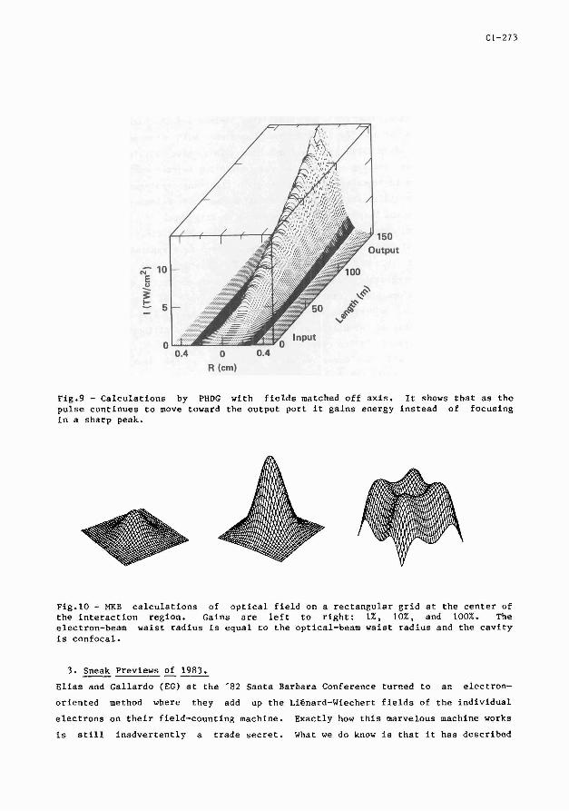
Fig.9 - Calculations by PHDG with fields matched off axis. It shows that as the pulse continues to move toward the output port it gains energy instead of focusing in a sharp peak.

Fig.10 - MKB calculations of optical field on a rectangular grid at the center of the interaction region. Gains are left to right: I%, lo%, and 100%. The electron-beam waist radius is equal to the optical-beam waist radius and the cavity is confocal.

3. Sneak Previews of 1983.

Elias and Gallardo (EG) at the '82 Santa Barbara Conference turned to an electron-

oriented method where they add up the Lignard-Wiechert fields of the individual

electrons on their field-counting machine. Exactly how this marvelous machine works

is still inadvertently a trade secret. What we do know is that it has described

C l - 2 7 4 JOURNAL DE PtlYSIQUE

fourier components of the optical fields for amplifier configurations in terms of

Gauss-Laguerre functions. We may begin to appreciate hov such machine may work by

regarding it as a special case of the retarded-time potential technique.

Colson and Richardson (CR), and Hiddleston, Colson and Richardson (HCR) have

reported progress at the '82 Santa Rarbara Conference with a rectangular-coordinate

fast-fourier-transform (FFT) propagation scheme. They have attained a technique

they describe as unitary (perhaps energy conserving in free space) and efficient

(for calculations in rectangular geometries with right-angle-polygon mirrors). CR

have used a parabolic profile for the electrons and have calculated mode patterns

for off-axis electron beams as well as the usual on-axis type.

Coffee, Lax, and Elliott(CLE) ( 2 5 1 describe propagation using a new

implementation of the well known fourier-Bessel technique applied to the paraxial

wave equation. In this CLE algorithm, the Hankel transforms are evaluated using

Gauss-Laguerre-integration (radial) locations and weights rather than by the quasi

fast Hankel transform (QFHT), the analogue of FFT, because of inefficiencies and

instabilities found in QFHT implementation. The finite mirror size was not included

in any of the multipass calculations, but I expect work by Elliott and Skokowski

will be incorporated in '83 to remedy this situation.

A. Bhowmik and R. Cover reported calculations for stable hole-coupled

resonators at a Rockwell International meeting in August 1982. The work is now

preliminary and uses simplified FEL models with a single gain sheet in a QFHT code.

D. Mathematical Ideas.

The mathematical formulation of the pulse propagation problem naturally divides

into two parts. The first part of the problem is the description of the

amplification process as the pulse moves through the interaction region. The second

part includes the cavity or resonator properties; it is concerned with what happens

to the pulse after it leaves the interaction region, up until it reenters the

interaction region; it describes the effect of the mirrors and apertures of the

system.

A summary of the theoretical work that has been done on the transverse

dependence (see below) is summarized in Fig.11. In principle all approaches began

with Maxwell's equations written in the wave equation form. The wave equation is a

partial differential equation having a source (differential source) that describes

the effect of the electrons or currents in incrementing the wave. Going from

Maxwell's equations to the paraxial wave equation has been discussed by Lax,

Louisell, and McKnight (261. The wave equation can also be written in an equivalent

form, as an integral over a relativistic volume source [ 2 ] , and this can be

expressed in terms of the well known retarded time potential. The retarded time

potential can be specialized to the case of a single electron in motion and gives

rise to the well known Lidnard-Wiechert potential for that electron. Less well

Fig.11 - Summary of theoretical work on optical quality showing logical flow from Maxwell's equations to various computations. Dashed lines represent work that either was not done or has not been reported.

known is the fact that the retarded time formalism, by using a number of paraxial

assumptions, can directly lead to the integral form utilized by Tang and Sprangle

[ 1 9 ] . They arrived at their integral form by way of the well known paraxial wave

equation.

This equation has many names, for instance, the parabolic wave equation, the

Gaussian wave equation, the quasi-optical wave equation, the envelope wave equation.

depending upon the emphasis one wishes to place on particular properties or uses.

The term paraxial emphasizes the physical requirement that the rays described by the

equation are all nearly traveling in the same (axial) direction. The term envelope

suggests that the modulation of the envelope must be slow compared to the carrier

frequency. All of these names refer to the following equation written for the

vector potential envelope,As,

JOURNAL DE PHYSIQUE

where ks= ws/c, and us is the carrier frequency, and V? is the transverse Laplacian.

The third major way the wave equation has been utilized is through the

free-space Fresnel-Kirchhoff propagator [12,24]. Although the results only apply to

free-space propagation, the formulation leads to an interpretation of the

propagator, and it is easy on a conceptual basis to generalize the interpretation to

include modification to rays by the effects of gain and phase from the source. This

method has been described as ad hoc phase and gain in Fig.11, but it has been shown

equivalent to the paraxial wave equation in Appendix A.

The three major ways the wave equation has been attacked are all closely

related to the paraxial wave equation. Although the details of the Lienard-Wiechert

potential method have not been made known, it is known that it may lead to a

Gauss-Laguerre formalism. Presumably this formalism is identical to that arrived at

by expressing the paraxial wave equation in cylindrical coordinates and finding its

free-space modes.

The paraxial wave equation expressed in cylindrical coordinates gives rise to a

(r,t) description, where r is the radial distance from the optical axis and t is a

time parameter describing the evolution of the pulse. The radial dependence can

arise due to rotational symmetry about the optical axis; the fact that we do not

have a z dependence comes about from taking a single z slice of the pulse and

ignoring coupling of the various z slices. The rectangular coordinate description

(x,y,t) involves breaking the transverse grid up into rectangles or squares rather

than rings.

There are three major ways the calculations can be implemented in either

rectangular or cylindrical coordinates. The first way is by finite differencing the

partial differential equations [6-81. The second way is to fourier transform

[13-181 (or Hankel transform in cylindrical coordinates). The third way is to

expand the solution in a series of functions having transverse dependence and

meeting boundary conditions in the transverse direction [9-11,251. In this later

category fall the boxes labeled Gauss-Laguerre, hybrid, partial waves, and

Gauss-Hermite. The finite difference boxes are labeled by A = > ; and the transform

methods are EFT and QFHT (the hybrid method may also be regarded as a transform

method).

As seen above there are many ways to formulate the general solution to the

paraxial wave equation . The initial conditions are the specification of the field

everywhere upon a plane. This may be done by specifying the field at a select N

points that become dense everywhere as N+m. Alternately we may choose N basis

functions and specify N coefficients. In either of these approaches we require the

additional physical condition that the field modulus be square integrable over the

initial plane; other than that we are free to choose the field at will.

From a mathematical point of view all of the representations are equivalent,

i.e. may be transformed back and forth into each other as N becomes infinite.

However some mathematical ideas can be expresses easier in particular

representations.

We can simplify the description of the solution to the paraxial wave equation

by choosing a representation in which free space propagation through any distance is

described by the idenity operation. The free-space mode coefficients are the

components of a vector in this representation, anc they don't change in traversing

free space.

We write the vector of coefficients for the incident field as E , and we

describe the generated, excited wave that gets added to the incident field as i. The value of ; is found by propagating the field and electrons through the

interaction region (the two board game described earlier) and depends on the

incident field in a non-linear way, so that we write :(E), to indicate the

functional relationship. The sum wave that leaves the interaction region is E+A(E),

and this wave reflects from two mirrors in the cavity whose total effect is

described by the linear operator M, a matrix. If we denote the new incident field

by E' to distinguish it from the old, we then have

as the description of our problem.

The second part of the problem involves specifying what the cavity or mirrors

do. We may categorize each of the schemes in terms of their mathematical

idealization. The most common scheme is shown as scheme number 1 in Table I. This

scheme takes the field vector on the n+l'th pass to be given by adding the excited

wave on the n'th pass to the incident wave and by multiplying by the mirror matrix.

Indeed this method follows the physics of the problem but is by no means the fastest

way to arrive at an equilibrium field vector, Em, assuming it exists. Scheme number

2 shown in the table is a relaxation technique, commonly used in numerical

algorithms, which takes the field on the n+l'th pass to be a weighted average of

that on the n'th pass and that predicted by scheme number 1. Here f is a free

parameter that is adjusted to achieve best convergence. These first two schemes are

explicit schemes because the field on the n+l'th pass depends directly on that of

the n'th pass.

The second group of schemes utilize the new value (n+l'th pass) of the field on

the right hand side of the equation and these are known as implicit schemes which

require solution of linear equations for their implementation. Scheme number three

is the IlKB [ 2 4 ] method (generalized to arbitrary order). That scheme utilizes the

JOUKNAL DE PHYSIQUE

Table I. I I I

Characterization Non-Linear Approach I 1 (driven by) I Algorithm Explicit

Schemes i.7 Like 1 but with relaxation

Schemes / 4 ( (old currents) ( Fn+l = M[E~+I + !(En) 1

1

En+l = f~. + (I - ~)M[E, + g ~ ~ ) I*

Implicit

Successive passes (old field)

3

Like 4 but

Error length I 2 Optimization/ 6 1 minimization h=min{l~-~[~+_h(E)]I }

E ~ + ~ = M[E, + @ " ) . I

"+l ' MCIEn+l 4- !(En) +

5

* f adjusted for best convergence t non-unity A is equivalent to A=l and a new reflectance

A times the old value because M is proportional to reflectance

= G(E)E

(old gain)

old (n'th pass) field values to determine the complex gain function matrix G; given

the gain an elgenvalue problem is solved for the field that would be self-consistent

were G the right value, The fourth scheme is similar to that used by Elliott [ 2 3 ]

and takes the currents to remain the fixed quantity based upon the old field. These

last two schemes have the advantage that when the current or gain is small, the

natural modes of the empty cavity appear. Scheme number 5 is similar to scheme

number 4, except that a linear correction term has been applied to ; the next order

taylor series term has been added making the expression for implicit itself. This

method and scheme number 6 in its usual implementation involve evaluation of xi(!,). A rule of thumb is that six place precision is required in evaluation of in order

to make gradient methods practical; this kind of precision is rarely seen in

calculations of FEL properties. Scheme number six is an optimization approach; it

is quite efficient in some implementations in that very few evaluations of ?(E) need

to be made.

t = +,+I + G(En)En+~ 1

higher order (En+l - En) -... VA(gn) 1

The introduction of the mathematical notation above has led to the suggestion

of several new schemes for achieving convergence of the mode problem, but it can

also be applied to advantage in characterizing the transverse mode problem as a

non-linear fixed-point problem. To do this we simply note that if an equilibrium

solution exists by numerical scheme number 1, we may write the problem as

We are also interested in the question of stability of this solution, and this

aspect can be studied by introduction of the error vector,

With this definition we may examine local stability in the neighborhood of a fixed

point Em by the taylor series expansion,

From this equation we see that the eigenvalues of !f(E,) determine stability. If

all the eigenvalues have modulus less than unity, then any error vector we may

construct as linear combinations of the eigenvectors will get smaller in modulus on

each successive pass.

What we have done here is to make a connection between a physical problem, the

free electron laser mode quality, and a well studied mathematical problem, the

non-linear fixed-point problem 1271. (A simple extension of the above arguments

also shows that (x,y,z,t) or (z,t) or (r,z,t) problems can be cast in a similar

fashion.) This fixed-point problem has recieved alot of attention and suggests a

general scenerio that has already been observed in the (z,t) problem. One usually

looks for a parameter of the physical problem that represents the drive of the

system. In the FEL problem the electron density or current may play that role. At

sufficiently low values of the driving parameter, the fixed point problem is

observed to exhibit stable solutions. As the driving parameter is increased, there

often comes a point at which the non-linear fixed point problem has no solutions.

What happens instead is that successive applications of f lead to limit cycle

behavior; i.e. the field vector varies between two solutions. Application of f to

one gives the other and vice versa. This switching between one solution and the

other is also known as a bifurcation of the solution. As the value of the parameter

increases further bifurcations can occur, and eventually at very high levels of the

JOURNAI. DE PHYSIQUE

parameter, the field vector will never reproduce itself. This kind of behavior has

not been verified numerically yet in the (r,t) mode quality schemes.

E. Digital Operations.

Given coders clever enough, And computers with the power of Hermes, We can calculate the world.

paraphrase of Archimedes

To show how quickly machines are gaining power, I have plotted the computer

power of the fastest digital calculator at the Los Alamos National Laboratory up to

the year 1980. The power is measured by the number of machine instructions per

second, where a floating point operation was arbitrarily defined to be three

instructions. These data are from Jack Worlton of the Computer Division; the points

for 1983 come from Chris Barnes also of Los Alamos, and the point labeled NSCP is

the projection of the National Super Computer Project in Japan. The graph (Fig.12)

shows that the trend for computers is to increase their power by a factor of ten

every four years, and the trend seems to be persisting into the future although

there is some disagreement about exactly how to extrapolate these data and what size

the error bars are.

Fig.12 - Computing power over the years at. Los Alamos. Computer growth and projections are consistent with a straight line fit that indicates computers increase their power a factor of ten in a little over four years.

10' - A&gu;tiig - lo0 1 I I I

1940 1950 1960 1970 1980 1990 Year

Those doing optical beam quality calculations will want to use the available

computer power or collaborate with those who have it. On the other hand, personal

computers may be useful for simple models, for building and polishing codes, and for

determining relevant physics. Computer codes are getting larger and more complex,

and rarely is it possible to present graphically all possible outcomes of a code.

We must pick and choose output diagnostics and input quantities in our numerical

experiment much the same way an experimentalist chooses the conditions he will study

and determines what measurements he will make. Our paraphrase of Archimedes

suggests that almost anything is computable, but in practice we require art in being

able to extract the relevant features of a problem and to attack those alone. The

skill of contriving a simple model having most of the physical features of the

problem is similar to the skill of an experimentalist who isolates a particular

physical effect from the influence of many others. Ideally the goal of

experimenting is to understand what is occuring and to be able to anticipate what

the results will be. It will be increasingly important for those running codes to

plan ahead and determine strategies to achieve that goal. It will also be important

to ensure that all the required skills in doing the numerical experiments are

assembled together in a working team.

Implementation of codes requires attention to the numerical algorithms in order

to avoid the introduction of spurious (non-physical) features. First we will

I I RAY PATH WITH! /

E M S 1 6 R I D I \ ' I I

/ /

/

,~$G,;ho' REFLECTION ! ORIGINAL GRID - 1 T;LATED 1

REAPPERANCE PER'ODlC OH O R I G I N A L A b C ~ ~ ~ ~ , ! , ~

I I I ORlGlNAl

GRlD

Fig. 13 - Ghost grid requirements. If the upper and lower ghost grids were not present, the boundary conditions on the original grid would result in spurious reflection or translation of rays.

JOURNAL DE PHYSIQUE

discuss the requirement of ghost cells in finite grid problems. Then assuming these

requirements are understood, we give a brief discussion of various algorithms.

The requirement of ghost cells arises from non-physical boundary conditions.

In Fig.13 we can see the idea of a criterion that can be applied a posteriori.

Suppose we have performed a calculation on an original grid and find that the

calculated pulse has a structure size of dimensions ds. (These arguments become

more complicated when focusing elements are present.) This structure will diffract

through an angle 8=X/ds, where X is the optical wavelength. In the case shown in

the figure, the structure is at the center of the original grid and it will diffract

at angle 8 and will be spread out to a width z8 after traveling a distance z. If the

spread is greater than the width of the original grid, additional grid points called

ghost cells are needed. Without ghost cells, the ray will impinge on the boundary

of the original grid. In a finite differencing code, the ray will reflect on the

original grid and change direction unlike the. real problem which has infinite

boundaries. With periodic boundaries in FFT algorithms, rather than reflecting on

the original grid, the ray reappears on the opposite boundary (suffering a

translation) but also in an unnatural fashion. The extent to which violation of the

ghost cell requirement will impact precision depends of course on the amplitude and

dimension of the diffracting structure relative to the rest of the pulse. Also,

depending upon the requirements, one may wish to have higher precision and more

confidence in the answer; in that case he might consider a new definition of the

defracting angle that is several times the above value.

Ghost cell requirements occur for FFT and finite differencing methods but not

for methods using a set of basis functions that meet the boundary conditions at m.

For finite difference methods B.R. Suydam has found that changing the boundary

conditions from reflecting to totally absorbing was not possible. However, Don

Prosnitz has suggested that the use of a grid with points that become spaced further

apart as the distance from the optical axis increases, ameliorates the ghost cell

requirements. In the EFT method the grid is fixed and ghost cells must be carefully

planned for.

The FFT technique is attractive because of its speed and the availability of

packaked routines that have been thoroughly tested. For a rectangular mesh of N by

N cells, the number of operations in the FFT is proportional to N~ log2N in going

one step. This few operations is sometimes an advantage, but there are several

things to keep in mind before deciding upon this algorithm. First ghost cells may

make N larger than in other methods. Second there may be symmetry present that can

not easily be taken advantage of in FFT. As an example, for a problem with

cylindrical symmetry it roughly requires N~ FFT points to do what can be done with N

points on a radial grid. Third sharp edges of mirrors are difficult to properly

model. Fourth another method may be more accessible and convenient to use. In

spite of these considerations, FFT should be given serious attention for problems

that are natural to rectangular coordinates.

Although the finite difference method has more flexibility in its grid, it is

somewhat more restrictive than EFT for free space propagation. With EFT one may

propagate the field arbitrarily far and get the same answer as if he took many

smaller steps, a definite advantage in problems with substantial free space

propagation. In the finite difference method an additional criterion occurs that

guarentees the solution will be sufficiently precise if the step size is small

enough. The criterion simply guarentees that the variation in the z (propagation)

direction should be small in a single step. For a smallest structure distance, ds,

in the transverse direction, the variation in the z direction occurs over a distance

that doubles the structure size i.e. z(X/ds) = ds or z = (ds)'/l. For a nearly

Gaussian mode 1281, this distance over which the area of the beam waist doubles is

known as the Rayleigh range or (twice this length) as the diffraction length.

Frequently, the criterion is that there are many steps in a Rayleigh range. Since a

FEL often has a length nearly equal the Rayleigh range, the criterion simply states

that many steps need to be taken in going through the interaction region.

In addition to the above criterion, the effect of gain and phase must give only

a small change to the field. For small gain FELs now in vogue this criterion

presents less of an obstacle than the free space criterion. When electron dynamics

are being calculated along with the optical propagation a step size is chosen in z

that describes the motion properly, and often it is the electrons that determine the

actual z step. In this case the interaction-region z step for the finite

differencing technique could be the same as that for FFT. Assuming a tridiagonal

scheme such as that used by Rensch 161, or Suydam [7], the number of operations

required for finite differencing of N radial grid points is roughly 3N per z step

and is actually less than an EFT technique (QFHT) would be for this problem.

The last technique we describe is to use free space modes as a set of basis

functions for the field. Like FFT there is no problem in taking arbitrarly large

steps in free space, and better yet there are no ghost cell requirements, but in the

interaction region the field must be evaluated at the locations of the electrons.

If there are N electron locations and N basis functions, that evaluation requires

2~~ numerical operations. Likewise, translation of the optical source at the N

electron positions into a source of mode coefficients also requires 2~~ operations.

(Another way to approach this problem is to work with grid quantities, but then

propagation requires a matrix multiplication having 2~' operations.) At first this

N' requirement might seem to rule out this technique, but upon closer inspection it

turns out for FEL problems that the number of basis functions in this technique is

considerably smaller than the number of radial grid points needed in finite

differencing. For instance, in the work reported by Elliott[Z3]only 20 basis

functions were required to get good eigenvalues for sharp-edged mirrors, whereas QS

was implemented with 200 radial cells, and in the QS technique the sharp-edged

mirrors had to be replaced with mirrors having a gradual fall-off of reflectivity.

Cl-284 JOURNAL DE PHYSIQUE

Another method closely related to that of free space modes is to use basis

functions that have the proper transverse boundary conditions. The requirements for

this approach include the condition that little variation in the field occurs in one

step, but as before with finite differencing this requirement is usually met

naturally in practice.

One final comment is that when we use groups of electrons at the same radial

locations at which the optical field is evaluated, the time required to do the

optical part of the problem is dwarfed by the time to push the electrons. Here

optical techniques should be chosen for their convenience rather than the number of

digital operations needed for their implementation.

Acknowledgements. - The author would like to thank: D. Quimby and J. M. Slater

for an advanced copy of their work, D. Deacon for inviting the topic C. Brau for

permitting the work to be done, John Goldstein and Paul Skokowski for suggested

improvements to the manuscript, Paula Adams and Joyce Schuster for assistance in

graphics, and Sarah Martinez for assistance in word processing.

APPENDIX A

We may see the practical equivalence of the MKB technique to the paraxial wave

equation by a simple argument. MKB relies upon the intuitive notion that with a

complex-gain coefficient, g+i6k E gc, which may be calculated, propagation is

described by,

where FP is the Fresnel propagator moving free space waves from the point x' where

Uo is evaluated, to the point 5 , where U is evaluated; here the integral over ds is

carried out along the straight line joining 5' to 5 . (Note that there appears to be

an inconsistency in the sign MKB use for 6k; their g-ibk convention is consistent

with exp(-ikz) waves whereas their propagator is consistent with exp(ikz) waves; we

are using the latter convention.) At the point 2 , FP is given by,

In the intuitive statement of the problem, the complex-gain integral occurs over the

same ray (straight line) that joins x to 5'; the statement is: To compute the

propagated field in the presence of an active medium that gives rise to a

complex-gain coefficient, we calculate the propagated field in the absence of gain

and multiply the result by the amplification of that ray (the amplification being

the complex exponential term appearing in Eq.Al). This statement is more

complicated than it might first appear in that the gain coefficient along a ray may

depend on the value of the field at all points along that ray; i.e., the field may

need to be calculated at all intermediate points.

To make the connection between MKB and the paraxial wave equation we need to

show that Eq.Al correctly includes the medium effects and does the free space

propagation. First we will verify that Eq.A2 satisfies the paraxial wave equation

and the boundary condition that as z+z', FP is the idenity operator. We proceed by

fourier transforming Eq.A2 from x and y to p and q. To achieve the interchange of

the order of integration we take w+w(l+i~+) and note that in this limit the new

inner integral converges. We complete squares in x and then y and note for Im(a) > 0, and (exp 18)'~~ = exp (i8/2),

00

I exp(iax2)dx = (in~a)'/~ . (A3) 4

We thus arrive at the tranformed equation:

where TV is V(x,y,z) fourier transformed in the first two variables. This

expression shows that the propagator in Eq.A2 meets the boundary conditions at z=z'

(note the difference with MKB), and it is an easy matter to show it satisfies the

transformed paraxial equation in free space,

where in real space p2=-a/ax2 and q2=-a/ay2.

The active medium effects are even simpler to establish. We develop the

partial differential equation for U by using values as given by Eq.Al at z and z+Az,

starting with Uo at z=0. We will remain at the same x,y point in forming the

partial derivative with respect to z, and will only indicate the axial location,

v.i.2. the z value. We subtract the following two equations,

Cl-286 JOURNAL DE PHYSIQUE

where we have further approximated the ray length by its projection on the z-axis;

this approximation is a paraxial assumption (MKB already have used a paraxial

approximation in using FP). By using the inverse of the first equation to

substitute out Uo in the difference equation we have,

Now in the limit that Az+0, the first term on the right side of Eq.A5 must give the

free-space terms, i.e. the transverse Laplacian terms, and the second gives the

gain term we were trying to establish, i.e.

_ = transverse Laplacian terms + u gc . a (A9)

The MKB method is thus seen to be practically identical to the paraxial wave

equation approach. MKB appears slightly more general in that they use the

ray-length in the gain expression rather than its projection onto the z-axis.

However, this is the only one of several uses of the paraxial approximation they

have eliminated, and it is not clear whether the others are more or less important.

In practice MKB also assume that the gain is small, making the above distinctions

unimportant for their application. Practically speaking the MKB approach is the

same as the paraxial wave equation.

References.

[l] Prosnitz(D.), Haas(R.A.), Doss(S.) and Gelinas(R.J.), Physics of Quan. Electronics, 1982, 9, 1047.

(21 Jackson(J.D.) , ~lassical Electrodynamics 2nd Edition, John Wiley and Sons Inc., New York, 1975.

[3] Kroll(N.M.), Morton(P.L.) and Rosenbluth(M.N.), Physics of Quantum Electronics, 1980, 7, 89. A more elegant version appears as Jason Technical Report, JSR-79-51, 1980.

[4] Moore(G.T.) and Scully(M.O.), Phys. Rev., 1980, g, 2000. [5] Colson(W.B.) and Elleaume(P.), Appl. Phys., 1982, E, 1. [6] Rensch(D.B.), Appl. Optics, 1974, 12, 2546. [7] Suydam(B.R.), LA-5607-MS, Los Alamos National Lab, Los Alamos NM, 1974. [8] Goldstein(J.G.) and Dickman(D.O.), LA-6955, Los Alamos National Lab, Los Alamos

NN, 1978. [9] Goubau(G.) and Schwering(P.), IRE Trans. on Antennas and Prop., 1961, 2, 248.

[lo] Kogelnik(H.) and Li(T.), Proc. IEEE, 1966, 54, 1312. [ll] Siegman(A.E.) and Sziklas(E.A.), Appl. Optics, 1974, 12, 2775. [12] Fox(A.G.) and Li(T.), Bell. Sys. Tech. J., 1961, 40, 489. See also

Eqs.(8.2.1) and (8.3.20) in Born(M.) and Wolf(E.), ~ r i n a ~ l e s of Optics, Pergamon, New York, 1965.

[13] Siegman(A.E.), Optics Lett., 1977, 1, 13. . [14] Agrawal(G.P.) and Lax(M.), Optics Lett., 1981, 6, 171. [15] Latham(W.P.) jr and Salvi(T.C.), Optics Lett., 1q80, 5, 219.

(161 Sziklas(E.A.) and Siegman(A.E.), Appl. Opt., 1975, 14, 1874. [17] Fleck(J.A.)jr, Morris(J.R.) and Feit(M.D.), Appl. Phys., 1976, 10, 129. (181 Goldstein(J.G.), LA-6833-MS, Los Alamos National Lab, Los Alamos NM, 1977. [19] Sprangle(P.) and Tang(C.-M.), Appl. Phys. Lett., 1981, 2, 677. Also: AIAA

Journal, 1981, 2, 1164. [20] Tang(C.-M.) and Sprangle(P.), Physics of Quantum Electronics, 1982, 9, 627.

Also: Proc. of the International Conference on Lasers '80, Dec. 15-19, 1980, Collins(C.B.) Editor, STS Press, McLean VA, 1981.

(211 Slater(J.M.), Quimby(D.) and Lowenthal(D.), Proc. of the International Conference on Lasers '80, Dec. 15-19, 1980, Collins(C.B.) Editor, STS Press, McLean VA, 1981. Also: Slater(J.M.) and Lowenthal(D.D.), 3. Appl. Phys., 1981, 52, 44.

(221 Quimby(D.C.) and Slater(J.M.), TEEE J. Quant. Elect., to appear 1982. [23] Elliott(C.J.), Physics of Quantum Electronics, 1982, 8, 531. (241 Mani(S.A.), Korff(D.A.) and Blimmel(J.), Physics of quantum Electronics, 1982,

9, 557. [251 ~ofTee(~.~.), Lax(M.) and Elliott(C.J.), IEEE J. Quant. Elect., to appear

1982. (261 Lax(M.), Louisell(W.H.) and McKnight(W.B.), Phys. Rev. A, 1975, 2, 1365. [27] Feigenbaum(M.J.), Los Alamos Science, 1980, 1, 4. [28] Yariv(A.), Quantum Electronics 2nd Edition, John Wiley and Sons Inc., New York,

1975, Chapter 6.6.