c copyright 2014 amittai axelrod
TRANSCRIPT

c©Copyright 2014
Amittai Axelrod


Data Selection for Statistical Machine Translation
Amittai Axelrod
A dissertation submittedin partial fulfillment of the
requirements for the degree of
Doctor of Philosophy
University of Washington
2014
Reading Committee:
Mari Ostendorf, Chair
Xiaodong He
Fei Xia
Program Authorized to Offer Degree:University of Washington Department of Electrical Engineering


University of Washington
Abstract
Data Selection for Statistical Machine Translation
Amittai Axelrod
Chair of the Supervisory Committee:Professor Mari Ostendorf
Electrical Engineering
Machine translation, the computerized translation of one human language to an-
other, could be used to communicate between the thousands of languages used around
the world. Statistical machine translation (SMT) is an approach to building these
translation engines without much human intervention, and large-scale implementa-
tions by Google, Microsoft, and Facebook in their products are used by millions daily.
The quality of SMT systems depends on the example translations used to train the
models. Data can come from a variety of sources, many of which are not optimal
for common specific tasks. The goal is to be able to find the right data to use to
train a model for a particular task. This work determines the most relevant subsets
of these large datasets with respect to a translation task, enabling the construction
of task-specific translation systems that are more accurate and easier to train than
the large-scale models.
Three methods are explored for identifying task-relevant translation training data
from a general data pool. The first uses only a language model to score the training
data according to lexical probabilities, improving on prior results by using a bilingual
score that accounts for differences between the target domain and the general data.
The second is a topic-based relevance score that is novel for SMT, using topic models
to project texts into a latent semantic space. These semantic vectors are then used


to compute similarity of sentences in the general pool to to the target task. This
work finds that what the automatic topic models capture for some tasks is actually
the style of the language, rather than task-specific content words. This motivates the
third approach, a novel style-based data selection method. Hybrid word and part-
of-speech (POS) representations of the two corpora are constructed by retaining the
discriminative words and using POS tags as a proxy for the stylistic content of the
infrequent words. Language models based on these representations can be used to
quantify the underlying stylistic relevance between two texts. Experiments show that
style-based data selection can outperform the current state-of-the-art method for task-
specific data selection, in terms of SMT system performance and vocabulary coverage.
Taken together, the experimental results indicate that it is important to characterize
corpus differences when selecting data for statistical machine translation.


TABLE OF CONTENTS
Page
List of Figures . . . . . . . . . . . . . . . . . . . . . . . . . . . . . . . . . . . iii
List of Tables . . . . . . . . . . . . . . . . . . . . . . . . . . . . . . . . . . . . iv
Chapter 1: Introduction . . . . . . . . . . . . . . . . . . . . . . . . . . . . 1
1.1 Difficulties with Data for Machine Translation . . . . . . . . . . . . . 1
1.2 Aspects of Text Variability . . . . . . . . . . . . . . . . . . . . . . . . 4
1.3 Dissertation Approach and Contributions . . . . . . . . . . . . . . . . 8
Chapter 2: Background . . . . . . . . . . . . . . . . . . . . . . . . . . . . . 11
2.1 Statistical Machine Translation . . . . . . . . . . . . . . . . . . . . . 11
2.2 Language Models . . . . . . . . . . . . . . . . . . . . . . . . . . . . . 23
2.3 Data Selection Methods . . . . . . . . . . . . . . . . . . . . . . . . . 25
2.4 Relationship to Prior Work . . . . . . . . . . . . . . . . . . . . . . . . 33
Chapter 3: Framework . . . . . . . . . . . . . . . . . . . . . . . . . . . . . 35
3.1 Data . . . . . . . . . . . . . . . . . . . . . . . . . . . . . . . . . . . . 35
3.2 Toolkits and Systems . . . . . . . . . . . . . . . . . . . . . . . . . . . 37
3.3 Pilot Studies . . . . . . . . . . . . . . . . . . . . . . . . . . . . . . . . 38
Chapter 4: Cross-Entropy-Based Methods . . . . . . . . . . . . . . . . . . . 42
4.1 Prior Work . . . . . . . . . . . . . . . . . . . . . . . . . . . . . . . . 42
4.2 Initial Work on Data Selection for SMT . . . . . . . . . . . . . . . . . 44
4.3 Extended Study of Cross-Entropy Difference Data Selection . . . . . 46
4.4 New Experiments for the TED Machine Translation Task . . . . . . . 51
4.5 Summary and Extensions . . . . . . . . . . . . . . . . . . . . . . . . 53
i

Chapter 5: Topic-Based Methods . . . . . . . . . . . . . . . . . . . . . . . 55
5.1 Topic Models in Language Modeling and Machine Translation . . . . 56
5.2 Topic Model Construction . . . . . . . . . . . . . . . . . . . . . . . . 58
5.3 Experiments . . . . . . . . . . . . . . . . . . . . . . . . . . . . . . . . 60
5.4 Analysis . . . . . . . . . . . . . . . . . . . . . . . . . . . . . . . . . . 74
Chapter 6: Style . . . . . . . . . . . . . . . . . . . . . . . . . . . . . . . . . 78
6.1 Background . . . . . . . . . . . . . . . . . . . . . . . . . . . . . . . . 79
6.2 Methods . . . . . . . . . . . . . . . . . . . . . . . . . . . . . . . . . . 81
6.3 POS Tag Analysis . . . . . . . . . . . . . . . . . . . . . . . . . . . . . 82
6.4 Experiments . . . . . . . . . . . . . . . . . . . . . . . . . . . . . . . . 85
Chapter 7: Cross-Method Comparisons . . . . . . . . . . . . . . . . . . . . 105
7.1 Using Selected Data . . . . . . . . . . . . . . . . . . . . . . . . . . . 105
7.2 Interpretation . . . . . . . . . . . . . . . . . . . . . . . . . . . . . . . 107
Chapter 8: Conclusion . . . . . . . . . . . . . . . . . . . . . . . . . . . . . 109
8.1 Experimental Summary . . . . . . . . . . . . . . . . . . . . . . . . . 109
8.2 Next steps . . . . . . . . . . . . . . . . . . . . . . . . . . . . . . . . . 112
ii

LIST OF FIGURES
Figure Number Page
4.1 MT results for data selection via random sampling, perplexity-based,and cross-entropy difference criteria. . . . . . . . . . . . . . . . . . . . 53
5.1 Heat map of topic weights for each 5-line chunk of the first talk inted-1pct-dev. The x axis is the topic ID, and the y axis is the locationof the chunk in the talk. . . . . . . . . . . . . . . . . . . . . . . . . . 65
5.2 Heat map of topic weights for each 5-line chunk of the second talk inted-1pct-dev. The x axis is the topic ID, and the y axis is the locationof the chunk in the talk. . . . . . . . . . . . . . . . . . . . . . . . . . 66
5.3 Heat map of topic weights for each 5-line chunk of the third talk inted-1pct-dev. The x axis is the topic ID, and the y axis is the locationof the chunk in the talk. . . . . . . . . . . . . . . . . . . . . . . . . . 66
5.4 Task granularity, in terms of number of topic vectors used to representthe task, and BLEU scores on ted-1pct-test for varying amounts ofselected data. . . . . . . . . . . . . . . . . . . . . . . . . . . . . . . . 68
5.5 Data selection using a topic model trained with and without in-domaindocuments. . . . . . . . . . . . . . . . . . . . . . . . . . . . . . . . . 70
5.6 Comparing topic-based and perplexity-based data selection methods. 72
5.7 Comparing topic-based and perplexity-based data selection methodswhen only 50 in-domain sentence pairs are available. . . . . . . . . . 74
6.1 Empirical frequencies of English Part of Speech tags in the TED andGigaword corpora. . . . . . . . . . . . . . . . . . . . . . . . . . . . . 83
6.2 Distance from each English POS tag to the line of equiprobability. . . 84
6.3 Using POS tags plus increasingly-frequent words in TED to select datavia cross-entropy difference. . . . . . . . . . . . . . . . . . . . . . . . 89
6.4 Empirical frequency thresholds of 10−4, 10−5, and 10−6 for vocabularywords with a minimum count of 20 in both TED and Gigaword. . . . 95
iii

LIST OF TABLES
Table Number Page
3.1 Available bilingual corpora . . . . . . . . . . . . . . . . . . . . . . . . 37
3.2 En-Fr bilingual corpora . . . . . . . . . . . . . . . . . . . . . . . . . . 38
3.3 Cross-task perplexities for 4-gram language models in English. . . . . 38
3.4 Cross-task perplexities for 4-gram language models in French. . . . . 39
3.5 Train/Dev/Test datasets for the En-Fr TED task . . . . . . . . . . . 40
3.6 SMT system performance when trained on 100% vs 98% of the TEDtraining data . . . . . . . . . . . . . . . . . . . . . . . . . . . . . . . 40
4.1 Bilingual and source side language model based data selection methods 52
5.1 Topic-based data selection methods vs. baselines on ted-1pct-test . 62
5.2 Task granularity, in terms of number of topic vectors used to representthe task, and BLEU scores on ted-1pct-test for varying amounts ofselected data. . . . . . . . . . . . . . . . . . . . . . . . . . . . . . . . 67
5.3 Data selection using a topic model trained with and without in-domaindocuments. . . . . . . . . . . . . . . . . . . . . . . . . . . . . . . . . 69
5.4 Comparing topic-based and perplexity-based data selection methods. 71
5.5 Comparing topic-based and perplexity-based data selection methodswhen only 50 in-domain sentence pairs are available. . . . . . . . . . 73
5.6 Top keywords for secondary topics in ted-1pct-dev. . . . . . . . . . 76
5.7 Top keywords for the primary topic in ted-1pct-dev. . . . . . . . . . 77
6.1 English POS tags with biased empirical distributions towards eitherTED or Gigaword. . . . . . . . . . . . . . . . . . . . . . . . . . . . . 84
6.2 Perplexity results for source-side data selection using POS LMs vs.lexical LM baselines . . . . . . . . . . . . . . . . . . . . . . . . . . . . 86
6.3 BLEU scores for source-side data selection using POS LMs vs. lexicalLM baselines . . . . . . . . . . . . . . . . . . . . . . . . . . . . . . . 86
6.4 Perplexity results for source-side data selection using hybrid LMs onPOS tags plus the most frequent words in TED . . . . . . . . . . . . 88
iv
6.5 BLEU scores for source-side data selection using hybrid LMs on POStags plus the most frequent words in TED . . . . . . . . . . . . . . . 88
6.6 Task corpus coverage of top 100 words in TED, by POS tag . . . . . 91
6.7 Perplexity results for source-side data selection using linguistically-motivated hybrid LMs . . . . . . . . . . . . . . . . . . . . . . . . . . 92
6.8 BLEU scores for source-side data selection using linguistically-motivatedhybrid LMs. . . . . . . . . . . . . . . . . . . . . . . . . . . . . . . . . 93
6.9 Perplexity results for source-side data selection using POS tags plusdiscriminative words. . . . . . . . . . . . . . . . . . . . . . . . . . . . 96
6.10 BLEU scores for source-side data selection using POS tags plus dis-criminative words. . . . . . . . . . . . . . . . . . . . . . . . . . . . . 97
6.11 English words with highest and lowest ratios of empirical frequency inthe TED corpus to its frequency in Gigaword. . . . . . . . . . . . . . 99
6.12 Comparing hybrid word/POS, topic-based and perplexity-based dataselection methods when only 50 in-domain sentence pairs are available. 100
6.13 Perplexity results for data selection using bilingual hybrid sequences. 102
6.14 BLEU scores for data selection using bilingual hybrid sequences. . . . 103
7.1 BLEU scores for two-model systems combining a system trained on1.35M sentences selected from Gigaword with a system using only 141kin-domain sentences. . . . . . . . . . . . . . . . . . . . . . . . . . . . 106
7.2 Number and coverage of the 47,661 words in the TED-98pct lexiconthat are included in the most relevant 900k sentences according tovarious selection methods. . . . . . . . . . . . . . . . . . . . . . . . . 107
v
ACKNOWLEDGMENTS
Roughly ten years ago I was unemployed, sitting in Toscanini’s in Central Square,
Cambridge, drinking coffee and working my way through a copy of Manning and
Schutze’s Foundations of Statistical Natural Language Processing. Going to grad
school to study machine translation seemed like a very reasonable idea. This year
I was also unemployed, sitting in Espresso Vivace in Capitol Hill, Seattle, drinking
coffee and writing my dissertation. The intervening decade has been, as described by
a Texan friend, “an exercise in cussedness.” Whether I paid a little too much attention
to Sinatra1 or Tennyson2 is debatable; what is certain is that I did not do this alone.
First and foremost, I thank Xiaodong He at Microsoft Research for his steadfast
encouragement and support, for having voluntarily and unhesitatingly given me so
much of his time and energy, and for patiently doing the steering as we chased ideas
together over the last four years. My gratitude is, appropriately, unquantifiable. I
would also like to thank Mari Ostendorf, who was an active mentor since I first arrived
on campus. Her experienced perspective has broadened my work, her attention to
detail has polished it, and I have learned much in the process. I am grateful for her
unwavering backing, even when I broke the lab’s espresso machine by accidentally
pouring water into the bean hopper. My sincere thanks go also to Katrin Kirchhoff,
whose support was instrumental during the early stages of this process.
My committee’s common factor was uncommon niceness. Howard Chizeck’s of-
fice was a much-needed – and much-used – sanctuary in the Electrical Engineering
1The record shows I took the blows - and did it myyyyyyyyyyyyy wayyyy” (Anka, 1969)
2“strong in will / to strive, to seek, to find, and not to yield” (Tennyson, 1842)
vi

building, and it also housed the departmental chacham. Someday I will laughingly
tell stories of the predicaments I escaped thanks to Howard waving his hand and
telling me “Don’t worry. What you’re going to do is the following...”. I am extremely
grateful for his wisdom, kindness, and kinship. Fei Xia did much to make me feel
welcome and relevant in the Linguistics department, and Archis Ghate of Industrial
& Systems Engineering taught INDE508, the most useful class I took at the UW. I
am thankful for their presence and assistance in the process leading to this document.
Radha Poovendran and Emily Bender were not on my committee – coordinating five
faculty is difficult enough – but I am no less grateful for their willingness to talk and
listen many times during my graduate career.
I have also benefited greatly from the generosity of Microsoft Research over the
last four years. They funded portions of this work, both directly and indirectly, and
were the first to adopt it. My thanks go to Will Lewis, Mei-Yuh Hwang, Jianfeng
Gao, and the Machine Translation, Natural Language Processing, and Speech groups
in the productive halls of Building 99.
I was glad to share a work environment at the U.W. with a number of people,
namely Alex Marin, Brian Hutchinson, Bin Zhang, Julie Medero, Nicole Nichols, and
Wei Wu, as well as Jeremy Kahn, Jon Malkin, Mei Yang, Alexei Alexandrescu, Alex
Stupakov, Kevin Duh, Stephen Hawley, and Tho Nguyen. Time with them outside
the department was well-spent. Also in the EE department, I am thankful to Lee
“nomad” Damon and Stephen Graham for keeping the process going.
I am appreciative of my global SMT support network, paricularly Chris Quirk,
Hieu Hoang, Juri Ganitkevich, Abhishek Arun, and Miles Osborne for being as ready
to listen during the last long years as to have a shifty pint. It is a pleasure to be able
to work in a field filled with friends; next round’s mine.
vii

My friends at the Climbing Club at the University of Washington provided me
with many days of mountain vistas and mental peace... and long, long days of
sweat, sunburn, shivering, fog, rain, rainy fog, bushwhacking, devil’s club, slide alder,
blowdowns, loose rock, boulders, scree, side-hilling, post-holing, avalanche hazards,
crevasses, Forest Service roads, mashed potatoes, and a steady source of cuts and
scrapes to go with carrying heavy things uphill. All of it was memorable, and better
than doing work. Most of it was fun, mostly in retrospect. The beer helped.
I am grateful to Jenny Hu, Danielle Li, Angela Hong, and Margarita Koutsoumbas,
for their assistance with Life, to Anna Folinsky, Charles Hope, Grace Kenney, and
Matthew Belmonte for just being $there, and to everyone else who has provided a
sympathetic ear during my troubles or a surface to sleep on during my travels.
This dissertation concludes my formal education. I would like to express my
appreciation to the following academics, both traditional and not: Jerome Lettvin,
Mrs. Cereida Morales, Alexander Kelmans, Carlos Rodriguez Fuste, Guihua Gong,
Richard B. “Dick” Dyer, Andras Kornai, Michael Collins, and David Yarowsky. They
shaped my path to this point, and their attention, effort, and patience made this
journey possible.
Finally, I am profoundly thankful to my family for their support and encourage-
ment, for indulging my curiosity, and for taking everything I’ve ever said or done in
stride for lo these many years. My love to Franklin Axelrod, Jean Turnquist, Ysaaca
Axelrod, and Barzilai Axelrod; I would not be where and who I am without them.
All errors, both personal and written, are of course my own.
viii

1
Chapter 1
INTRODUCTION
1.1 Difficulties with Data for Machine Translation
A Statistical Machine Translation (SMT) system is a statistical framework that learns
by data-driven methods to translate text from one human language to another, and
then can automatically perform such a translation. The performance of any SMT
system depends in large part on the quality and quantity of the bilingual data over
which the system is built. All-purpose translation systems are the holy grail of ma-
chine translation research, and much work goes into acquiring more translated docu-
ments to feed into the system and thereby increase its coverage. A translation system
trained on a sufficiently general corpus could translate a newspaper editorial, status
updates on Facebook, and the latest match reports from the Italian “Serie A” football
league. However, there is much need for a translation system that works well for a
particular usage or task. Some of these tasks are ones for which not much available
bilingual data exists. Perhaps the subject is too recent (e.g. a new scientific discov-
ery), has an inherent size limit (e.g. the works of a dead author), is simply sparse
(e.g. few Chinese cookbooks are bilingual), or has restrictions on its use (e.g. a large
publisher owns bilingual data, but declines to license it externally).
We can (and do) use a general-purpose translation system to translate task-specific
documents, but we wish to do better. The price for a general-purpose system’s breadth
includes widely scattered errors from a lack of context for the translations; the system
might have occasional trouble differentiating which sense of a word is more relevant,
such as whether “bank” refers to the financial institution or the edge of a river.

2
Such errors would be localized and not consistently made. By contrast, a targeted
translation system should do well at the task of interest. For example, a translation
system designed specifically to help travelers could use the context of the task to
translate the word “train” more often as a noun than as a verb.
However, this task-specific information makes the targeted system less useful as
an all-purpose system. Feeding an article about how sportsmen “train” to a system
expecting tourism-related requests could lead to a translation systematically and er-
roneously discussing railroads instead of match preparations. If a general system is
said to have average translation performance on all inputs, then an ideal task-specific
system would have higher performance on task-related text but possibly lower perfor-
mance on everything else. This tradeoff might seem Faustian, except we inherently
prioritize performance on the current task above all else: when trying to reach the
correct platform for a train which leaves in three minutes, one might not be overly
concerned with how well the translator can read the sports pages.
Machine translation system performance is dependent on the quantity and quality
of available training data. The conventional wisdom is that a lot of data is good, and
more data is better: the larger the training corpus, the more accurate the model
can be. These adages are backed by evidence that scaling to ever larger data shows
continued improvements in quality, even when one trains models over billions of n-
grams (Brants et al., 2007). Likewise, doubling or tripling the size of tuning data can
show incremental improvements in quality as well (Koehn and Haddow, 2012). The
trouble is that – except for the few all-purpose SMT systems – there is never enough
training data that is directly relevant to the translation task at hand. Not all data
is equal, however, and the kind of data one chooses depends crucially on the target
domain. Even if there is no formal genre for the text to be translated, any coherent
translation task will have its own argot, vocabulary or stylistic preferences, such that
the corpus characteristics will necessarily deviate from any all-encompassing model of
language. For this reason, one would prefer to use more in-domain data for training.

3
This would empirically provide more accurate lexical probabilities, and thus better
target the task at hand. However, parallel in-domain data is usually hard to find, and
so performance is assumed to be limited by the quantity of domain-specific training
data used to build the model. Additional parallel data can be readily acquired, but
at the cost of specificity: either the data is entirely unrelated to the task at hand,
or the data is from a broad enough pool of topics and styles, such as the web, that
any use this corpus may provide is due to its size, and not its relevance. The task
of domain adaptation is to translate a text in a particular (target) domain for which
only a small amount of training data is available, using an MT system trained on
a larger set of data that is not restricted to the target domain. We call this larger
set of data a general-domain corpus, in lieu of the standard yet slightly misleading
out-of-domain corpus, to allow a large uncurated corpus to include some text that
may be relevant to the target domain.
If the amount of in-task data is limited, then we must mine additional relevant
data from the many documents used to train the general-purpose system. The goal of
this work is to provide a structured way of quantifying how relevant these documents
are to the target domain, and then using the most relevant general-purpose data
to build a better in-domain translation system. One might believe that all training
data is useful for training a language model (LM) or a statistical machine translation
(SMT) system. In theory, all inaccurate, noisy, or irrelevant data should get minimal
probability, and so at worst some data might make no discernible contribution to
the model. In practice, however, adding data that is particularly irrelevant (e.g. ill-
matched or noisy) to the target task to the training corpus degrades the quality of
the resulting models.
Many existing domain adaptation methods fall into two broad categories. Adap-
tation can be done at the corpus level, by selecting, joining, or weighting the datasets
upon which the models (and by extension, systems) are trained. It can be also
achieved at the model level by combining multiple translation or language models

4
together, often in a weighted manner.
An underlying assumption in domain adaptation is that a general-domain corpus,
if sufficiently broad, likely includes some sentences that could fall within the target
domain and thus should be used for training. Equally, the general-domain corpus
likely includes sentences that are so unlike the domain of the task that using them to
train the model is probably more harmful than beneficial. One mechanism for domain
adaptation is thus to select only a portion of the general-domain corpus, and use only
that subset to train a complete system.
There is no current consensus as to a good way to filter, weight, or target the
training data effectively for the purposes of downstream LM or SMT applications.
Common methods are to discard data – often using a perplexity-based measure –
or to construct mixture models of the task domain corpus and the additional data.
There is thus a need for this dissertation’s work on using existing resources more
judiciously to produce better targeted statistical machine translation systems.
1.2 Aspects of Text Variability
Several factors contribute to making text relevant for a task, and we explore them in
this work. We use translation domain to mean the set of things one could translate
within some human-defined scenario, such as “traveling”, “following E.U. parliamen-
tary proceedings”, or “watching a movie”. A translation task is a specific set of things
that have or will be translated within the scenario, such as “the words on that street
sign”, “vi er pa vej mod verdensherredømmet”, or “Frankly, my dear, I don’t give a
damn.” One only works with extant data in a research setting, so the domain and the
task both reduce to the available data. We therefore use the terms task and domain
interchangeably in this work.
A domain-specific corpus has some particular text and characteristics related to
the application. These characteristics are reflected in the corpus’ lexical specificity,
or the choice of words and phrases used. We refer to the corpus as text because

5
we are interested in translation – a text-to-text problem – even though the text
might be from transcribing speech or performing optical character recognition on an
image. We abstract away the text’s origin because provenance of the data has an
effect on the content of the corpus, but not on the method by which the translation
is performed. A general-domain corpus ought to contain data spanning all or most
domains, which is difficult to verify. We use the safer mixed-domain to mean a corpus
that is heterogeneous with respect to domain, with no further implications of coverage.
There are other ways to describe a corpus besides its domain. Domain is what the
text in the corpus is for, but topic is what it is about. Topics are clusterings of related
language, tightly coupled with content words, and humans can interpret those clusters
as being thematic, like “baseball”, “computer vision”, or “global health”. Topics can
span across domains, as “health” might be related to both TED talks (as global
health), and travel (as emergency clinics). Similarly, domains often span multiple
topics, as “travel” covers airports, traffic signs, and conversations with strangers.
Both domains and topics are characterized using the words found in the corpus, so
they are not entirely independent. Particular human scenarios (e.g. booking a flight,
listening to a talk) drive most translation settings and corpus acquisitions, so corpora
are most commonly single-domain and multiple-topic. Such a multiple-topic corpus is
said to exhibit topical variety or be topically heterogeneous, as opposed to a topically-
homogeneous corpus which only contains text pertaining to a single topic.
Language is used to communicate, and thus we might also consider the social
context in which it is used, in addition to what the text is for, and what it is about.
We refer exclusively to text in this work, but the terminology we describe is sufficiently
general to cover both speech and text. The field of sociolinguistics studies linguistic
variation and its correlation with sociological categories, so we have need for some
sociolinguistic textual descriptors. The notion of “social context” is broadly defined,
and so the commonly-used terms of register, style, and genre are as well.
A text is “a passage of discourse which is coherent in these two regards: it is

6
coherent with respect to the context of situation, and therefore consistent in register
and it is coherent with respect to itself, and therefore cohesive” (Halliday and Hasan,
1976). Register is a variety of language used in a particular social setting or for
a particular purpose. First used by Reid (1956) as a way to differentiate linguistic
variations between users from variations between uses. ISO standard 12620 defines
a list of 11 registers that can be used in natural language processing, including di-
alect, facetious, formal, technical, and vulgar. Quantifiable linguistic differences, such
as relative clauses, between registers are “quite frequent in official documents and
prepared speeches but quite rare in conversation” (Biber, 1993).
Style is used to describe the association of language with particular social mean-
ings, such as group membership, beliefs, or personal attributes. It is generally as-
sociated with the social context, and appears to subsume register. Style could be
defined only within a social framework (Irvine, 2002), or it could also incorporate
personal stance-taking, indicating the position of the speaker with respect to an ut-
terance (Kiesling, 2005). Style can be syntactic, lexical, or phonological. We will
explore the first two; the latter is well outside the scope of this work. Written style
can arguably also be extended to include typos, capitalization, formatting, and other
information that is particular to the author and the medium in which the text is pro-
duced (Koppel and Schler, 2003), but that is also beyond the limits of the problem we
are considering. Labov (1984) examined the social stratification of English, relating
language with social classes, and defined styles as ranging along a single dimension,
measured by the amount of attention paid to speech. He declared “There are no
single-style speakers”, because we shift sociological contexts depending on whom we
are communicating with.
Measuring attention to speech is often impractical, but formality can be used as
an approximation. For example, Joos (1961) claims there are five levels in spoken
English. These are:

7
1. Static: The wording is always exactly the same (e.g. the Miranda warning).
2. Formal: One-way participation, with no interruptions (e.g. presentations).
3. Consultative: Two-way, interruptions allowed (e.g. doctor/patient).
4. Casual: In-group friends. Slang, interruptions, ellipsis common.
5. Intimate: Private, intonation is more important than wording or grammar.
We will use style as a criterion in this work, as it is more intuitive to us than register,
though both are similar.
A third sociolinguistic aspect of language is its genre. Genre and register are
sometimes used as synonyms (Gildea, 2001) – but genre is more concerned with to
the communicative purpose of a text (Webber, 2009). Examples of heteroglossia,
or speech genres (Bakhtin, 1975), are “formal letter”, “grocery list”, and “personal
anecdote”. Classic examples of genres are found in literature (novel, poetry, comedy,
epic, etc). Genres are neither necessarily static nor disjoint: tragicomedies grew out
of the tragedy and comedy genres. Genre is claimed to be determined by four things:
linguistic function, formal traits, textual organization, and relation of communicative
situation to formal and organizational traits of the text (Charaudeau and Maingue-
neau, 2002). Alternatively, it is “any widely recognized class of texts defined by some
common communicative purpose or other functional traits, provided the function is
connected to some formal cues or commonalities and that the class is extensible”
(Kessler et al., 1997).
There are demonstrable linguistic differences between genres, such as “S-initial
coordinating conjunctions (‘And’, ‘Or’ and ‘But’) are a feature of [...] News but not
of Letters” (Webber, 2009). A more approachable example is that an occurrence of
the word pretty is “far more likely to have the meaning ’rather’ in informal genres
than in formal ones” (Kessler et al., 1997), though it blurs any distinction between
genre and style. However, genre seems to be a broader and higher-level set of text
classifications than is needed to cover individual standard machine translation tasks.
We use the term style and not genre as our third focus, along with domain and topic.

8
A domain-specific corpus may also include variation on topic or style, but is not
implied to do so. Similarly, a topic-specific corpus may cover a range of domains or
styles, and a style-specific corpus may span a variety of topics or domains, but they do
not have to. With the many possible defining characteristics for an in-domain corpus,
there are equally many ways of defining the similarity between the target domain
(as defined by the available in-domain corpus) and a sentence from a mixed-domain
corpus. Our end goal is to improve statistical machine translation, and so we examine
three facets of language that are of interest to SMT: domain, topic, and style. These
characterize what the text in a translation task is for, what it is about, and how it is
expressed. Each of the three approaches in this work addresses one of these facets.
Each of them also examines different aspects of the words that are used in a text:
domain considers all the words in each sentence equally, topic primarily uses the
cooccurrence of content words, and style is related to the proportion and sequence of
words and word categories, such as content and function words, used to construct the
text. These three approaches overlap in their consideration of the words in a task,
and so addressing style or topics may help select a better lexical distribution as well.
1.3 Dissertation Approach and Contributions
We will quantify the different factors that lead to domain differences using cross-
entropy based similarity measures, a topic distribution vector distance, and structural
similarity scores. We examine the pool of additional data on a sentence-by-sentence
basis or in small chunks, but these methods could easily be adapted to work on larger
or smaller textual units. Our major contributions are novel methods of selecting data
for statistical machine translation. We build targeted MT systems using the most
relevant data from the mixed-purpose corpus, according to the different notions of
relevance. We evaluate the sub-selected systems based on whether they outperform
the general system on the domain of interest. We also test whether these targeted

9
models can be improved further via their combination with the existing baseline
models to create an augmented task-specific translation system. We propose using
these mechanisms in principled, generalizable ways to efficiently use available training
data to build SMT systems that are better suited for translating task-specific texts.
Our work spans several facets of natural language processing, primarily language
modeling, statistical machine translation, and topic modeling. Chapter 2 presents
the scientific background that frames this work, as well as an overview of previous
approaches to quantifying textual relevance or selecting data for machine translation.
We describe our experimental framework in Chapter 3, and provide pilot studies
on cross-task modeling degradation that illustrate the problem we wish to address.
Chapter 4 lays out our pioneering work on cross-entropy based data selection
methods for statistical machine translation. We explain and then apply a relevance
metric from language modeling to SMT, and show that it can be used to improve
translation performance. We then present our extension to this metric that further
improves on the state of the art by taking advantage of the bilingual nature of machine
translation training data.
We next compute relevance by focusing on content or topical words in Chapter 5,
with the idea that these are the most important words to translate in a sentence. Tthe
topic-based method is more effective than the word-based cross-entropy difference
method only when the amount of in-domain data is extremely small. However, we
do find evidence to support using a fine-grained a representation of the target task to
capture topic dynamics, and the content of the automatically extracted topic clusters
directly motivates style-based approaches.
In Chapter 6, we analyze the impact of using particular classes of words as indi-
cator features for data selection, and show that words that bias towards one corpus
or the other can be used effectively to identify relevant sentences, even with small
amounts of in-domain training data.
10
We analyze the three data selection approaches in Chapter 7, with an eye towards
showing the practical usefulness of the selected data. We also find another benefit of
the data selection methods, which is an increase in in-domain coverage via a reduction
in out-of-vocabulary words.
Finally, we summarize our results in Chapter 8 and discuss future directions.

11
Chapter 2
BACKGROUND
Our goal is to match additional training data to the scenario for which the trans-
lation system is being used. This is a common real-world situation, where there is a
limited amount of task-relevant data, but we have additional un-curated data at our
disposal. This chapter is a summary of the historical and current research landscape
relating to our application of data selection methods to statistical machine translation
(SMT). Section 2.1 is a primer on modern statistical machine translation, including
the methods we use for our experiments. Section 2.2 explains n-gram language mod-
els (LMs), which we use both as a component of SMT systems and as a separate
framework for generating and using probability distributions from corpora. Section
2.3 describes three axes along which to measure corpus similarity that can be used
for data selection: lexical, topical, and stylistic. Section 2.4 describes how our work
fits with the context provided in the first three sections.
2.1 Statistical Machine Translation
Statistical Machine Translation is the study of using a probabilistic framework to
translate text from one human language to another. The process for building such
a system relies on a parallel corpus, which is a set of sentences in the first language
and their corresponding translations in the other. Training an SMT system yields
a set of probabilistic models that have been automatically induced from the parallel
corpus. These models are then used by a decoder to perform the actual translation of
previously-unseen documents. Among the models learned during the training process
are a translation model (TM), which quantifies the correspondence between words

12
and phrases in the two languages, and a language model (LM), which measures the
fluency of the output language. The quality of an SMT system is most commonly
measured via the BLEU score of its output. Language models have their own common
evaluation metric, perplexity, because language models are also used in other fields,
such as Automatic Speech Recognition (ASR). The details of language models are
discussed in Section 2.2, after we first explain statistical machine translation.
2.1.1 MT Evaluation
The goodness of machine-translated output would ideally be judged by humans. How-
ever, this is subjective, and time-consuming (thus expensive). Machine translation
research relies on having automatic, fast, cheap, and deterministic methods of evaluat-
ing and ranking translations. This is easiest for sentences which already have human
translations to compare against. Such translations are called reference translations.
The most common automatic translation metric for MT output is BLEU (BiLingual
Evaluation Understudy), developed by IBM (Papineni et al., 2002).
BLEU rewards MT outputs that match the reference in word choice, word order,
and length. It measures the number of matching n-gram sequences between the MT
output sentence and the reference. As a precision-oriented metric, BLEU considers
the ratio of matches to the total number of n-grams in the reference translation.
To prevent over-generating simple words (e.g. “the the”), this n-gram precision is
clipped to reward only as many matches in the output as there are occurrences in the
reference, as in this example from (Papineni et al., 2002):
Candidate : the the the the the the the.
Reference : The cat is on the mat.
Modified Unigram Precision = 2/7.
For an n-gram g, let #(g) be the number of times g appears in some MT output
O containing sentences o1, o2, .... Let #clip(g) be the number of times g appears in
the reference translation for some oi. Then the modified n-gram precision pn of O is:

13
pn =
∑oi∈O
∑g∈oi #clip(g)∑
oi∈O∑
g∈oi #(g)
The standard implementation of BLEU considers n-grams for order 1 ≤ n ≤ 4,
each of which has can associated n-gram precision. These precisions are combined by
taking their geometric mean:
4∏n=1
(pn)14 = e
∑4n=1
14log pn
Note that the denominator of pn is the total number of n-grams produced in the
MT output O, which inherently rewards systems that produce shorter outputs by only
translating the easy parts of a sentence. To counter this, BLEU contains a Brevity
Penalty (BP), which penalizes outputs that are shorter than the reference. If the
entire output O has length |O| and the reference set has total length |R|, then the
brevity penalty is:
BP =
1 if |O| > |R|.
e(1−|R||O| ) otherwise.
BLEU is the product of the Brevity Penalty and the geometric mean of the mod-
ified n-gram precisions:
BLEU = BP · exp(4∑
n=1
1
4log pn ) (2.1)
BLEU does have some disadvantages. It can only handle translation variety when
“multiple human translators with different styles are used” (Papineni et al., 2002).
The BLEU score also has the disadvantage of being 0 if any of the n-gram precisions
are 0, due to taking the geometric mean of the n-gram scores. As such, BLEU can
only attempt to match human evaluations when averaged over a test corpus, and not
on a sentence-by-sentence basis. Other metrics such as TERp (Snover et al., 2009)
and METEOR (Denkowski and Lavie, 2011) have been proposed to address aspects

14
of BLEU’s shortcomings. However, BLEU’s ease of use on a test set makes it the
dominant metric for machine translation, and so we use it here as well.
Statistical significance is not straightforward to assess for SMT output. BLEU
scores vary complexly with small changes in the system output. BLEU is not com-
puted on a per-sentence basis, and so normal methods of computing significance and
confidence intervals are not readily applicable. Koehn (2004) used bootstrap resam-
pling to determine the statistical significance of BLEU scores, but the accuracy of
this has been criticized (Riezler and Maxwell III, 2005). The statistical significance
of sets of pairwise comparison of SMT output can be determined, but the collection
of the necessary human judgements (Koehn and Monz, 2006) is beyond the scope of
this work.
2.1.2 Translation Models
Modern statistical machine translation started with the description by Brown et al.
(1990) of a set of generative models (known as the IBM Models), for automatically
translating sentences from French into English. Although current SMT systems are
more sophisticated, the IBM models are an intuitive introduction to the field. The
IBM models regard a French sentence F as an encoding of an English sentence E when
translating from input language F → E. This means that the probability P (E|F ) of
sentence E being an intended translation of F can be expressed using Bayes’ rule:
P (E|F ) =P (E) · P (F |E)
P (F )
The denominator P (F ) is independent of any possible hypothesized translation E.
Therefore the single most likely translation hypothesis E can be produced by maxi-
mizing the numerator:
E = argmaxE
P (E) · P (F |E) (2.2)

15
The term P (F |E) is known as the translation model probability, and can be further
decomposed via the chain rule into the product of the translation probabilities of
smaller phrases in P to ones in E. P (E) is called the language model probability, and
reflects the likelihood that E is a fluent sentence in the output language.
In phrase-based statistical machine translation, sentences are considered to be se-
quences of phrases, which are themselves sequences of contiguous words (regardless
of linguistic content) (Koehn et al., 2003). To translate (or decode) an input sen-
tence, a phrase-based SMT system splinters the sentence into many possible overlap-
ping phrases. Translation is done greedily. At each step, the next-best untranslated
phrases are selected, translated, reordered, and placed into the output one at a time
to construct the translation. In general, when we refer to “SMT” in this work, we
mean phrase-based SMT.
The set of phrase pairs are acquired heuristically (Koehn et al., 2003) from a par-
allel corpus whose words have been aligned, such as by GIZA++ (Och and Ney, 2003)
or fast align (Dyer et al., 2013) . The relative frequencies of the aligned phrase pairs
in the training corpus, as well as the relative frequencies of the aligned phrase pairs to
the monolingual phrase counts, are the basis for computing translation probabilities.
The phrase translation probability p(e|f) of a source phrase f to a target phrase e is:
p(e|f) =Count(e, f)
Count(f)(2.3)
In the generative model, all phrases in F are translated to their targets indepen-
dently of each other. Switching from a generative to a discriminative log-linear model,
as in (Och and Ney, 2002), allows modern statistical MT systems to use any number of
models or features, even overlapping ones, to select the best translation for a phrase.
Log-linear models define a relationship between a set of features h of the parallel
data (E,F ), and the translation function P (E|F ) (Lopez, 2008). This relationship
is not inherently a probability, unlike in the generative models, and so it is usually
normalized. A feature can be any function whatsoever, as long as it assigns some

16
non-negative value to every bilingual phrase pair. The IBM model derived scores
are often used as features in log-linear translation models, as well as the language
model score P (E), but “number of capitalized letters” could be also a valid feature.
Each feature receives a weight λ which determines (or reflects) the importance of the
feature for translation. The best hypothesized translation E for a log-linear model,
analogous to Equation 2.2, is:
E = argmaxE
P (E|F ) (2.4)
This time we decompose into a log-linear combination of weighted features:
P (E|F ) =1
Z· exp(
∑m
λm log hm(E,F ) ) (2.5)
The use of arbitrary features h means we can construct the Z term to normalize the
resulting score so that it sums to unity:
Z =∑E
exp(∑m
λm log hm(E,F ) ) (2.6)
The features h(E,F ) are usually defined directly to be logarithmic, to reduce com-
putation and simplify the notation:
Z =∑E
exp(∑m
λm · hm(E,F ) ) (2.7)
Many translation model features have been proposed, but Moses (Koehn et al.,
2007), the standard framework for phrase-based SMT, uses eight by default. These
features are a language model, a reordering model, a length feature, and a phrase-
based translation model (5 features), and are computed as follows:
1. The language model feature is based on the empirical probability of seeing the
phrasal units in the training data. We describe it shortly, in Section 2.2.

17
2. The reordering model feature characterizes the likelihood of local phrasal rear-
rangement in the translation E. More rearrangement is likely for translating
German into English, where the verb moves, than for translating closely related
languages, such as French into Spanish, where the word order is already correct.
The default reordering model (Koehn et al., 2003) is linear on the number of
phrases jumped during translation. Let ai be the start position of the input-
language phrase that was translated into the ith output-language phrase, and
bi−1 is the end position of the output phrase translated into the (i− 1)th output
phrase. The distortion cost of this translation sequence according to the linear
distortion model is:
di = (ai − bi−1)
The distortion cost feature hdistortion(E,F ) of the sentence pair is:
hdistortion(E,F ) =∑i
(di)
There is a hard limit on reordering distance, called the distortion limit, whereby
two phrases that are very far apart in the sentence cannot translate each other.
This hard constraint prevents the search space from expanding exponentially.
There are also lexicalized reordering models, such as by Koehn et al. (2005) and
others, that measure the reordering likelihood on a phrase-by-phrase basis.
3. The word penalty feature discourages translations that are extremely short –
preferred by the language model – by adding a constant cost w = elength(w) per
word generated. The word penalty feature for the sentence thus only depends
on the length of the output:
hlength(E,F ) = elength(E)
A negative feature weight λ biases system output towards longer sentences.

18
The remaining features are called the translation model, and are usually stored
together as a phrase table, which is a list of phrases in one language, their transla-
tions, and a set of scores that reflect the likelihood of that phrase pair being a good
translation. Each of these features receives their own weight in the log-linear transla-
tion framework. The five common features used by phrase-based SMT are the phrase
probability for translating from the input language to the output language (the for-
ward direction), the phrasal probability of translating from the output language to the
input language (the backward direction), the forward and backward lexical transla-
tion probabilities, plus a phrase penalty. These features are defined over phrases, not
sentences, as they are used to construct the translation hypotheses, and so a feature’s
value for a sentence is the product of the scores of the phrases for the best-scoring
partition of the sentence into phrases, which is equivalent to the sum of the log of the
phrase scores.
4. The forwards phrase translation probability feature hFPP is the product of all
the phrase translation probabilities in Equation 2.3 for a specified partition of
the sentence F into K phrases:
hFPP (E,F ) =K∏k=1
p(ek|fk) (2.8)
5. The forwards lexical translation probability of a phrase pair depends on the
empirical word translation probability of each input word wfi to its aligned
output word wej :
p(wej |wfi) =Count(wej , wfi)
Count(wfi)(2.9)
The lexical translation probability for an input phrase with I words is the
average word translation probability:

19
lex(e, f) =1
I
∑i
p(wej |wfi) (2.10)
The forwards lexical translation probability feature hFLP can be defined in a
variety of ways; a common method is to set it to the product of all the forward
lexical translation probabilities for the partition of the source sentence F into
K phrases:
hFLP (E,F ) =K∏k=1
lex(ek, fk) (2.11)
6. The backwards phrase probability feature is the same as the forwards phrase
probability, except computed in the reverse direction:
hBPP (E,F ) = hFPP (F,E)
Thus the backwards features are functions of the phrases in the other side of
the parallel data, and they cover the phrases in a partition of the output-side
sentence E.
7. The backwards lexical probability feature is similarly the forwards lexical trans-
lation probability computed computed in the reverse translation direction:
hBLP (E,F ) = hFLP (F,E)
8. The phrase penalty feature is, like the word penalty feature, a constant cost
during decoding. The phrase penalty is accumulated per phrasal unit in the
partition of E into phrases, and each phrase has a cost of e. This corresponds
to a linear cost of +1 per output phrase used to translate an input phrase.
One SMT system can use multiple translation or language models in parallel, and
multiple SMT systems can be assembled via system combination to provide improved

20
translations. After all the models are trained, the feature weights λ for each feature
h need to be set so as to balance the features to maximize the quality of the out-
put (measured by BLEU score). This optimization procedure is an active research
problem, but one widely-adopted approach over a small number of features, such as
the ones described, is to perform Minimum Error Rate Training (MERT) (Och, 2003)
against a held-out dataset.
2.1.3 Hierarchical Phrase-Based Translation Models
Phrase-based SMT systems can learn local word reorderings such as the verb and
adjective swap from Spanish (“el gato negro”) to English (“the black cat”), but only
for phrase pairs that were seen during training, and cannot span more than n con-
secutive words. Long-distance reordering can only happen during decoding, and is
limited by the distortion limit. Hierarchical phrase-based translation (Chiang, 2007)
lies between phrase-based methods and the syntax-based systems described below, in
Section 2.1.4. Like phrase-based SMT, a hierarchical system fundamentally consists
of mappings from word chunks in one language to another.
In a hierarchical system, the translation model contains context-free grammar
rules that are formally syntactic, but do not use linguistic syntax. The difference is
that only one non-terminal symbol (“X”) is used in lieu of the standard linguistic
syntax. The phrases and rules are extracted from the word-aligned sentences in the
parallel training corpus, without any syntactic parsing. The right-hand side of a rule
is allowed to contain at most two nonterminals, but may contain several terminals
in both languages – a phrase and its translation. Recall that the leaves of a parse
tree are the terminals, or words, and the non-terminals are all nodes higher up in the
tree. Furthermore, non-terminals must be separated by a terminal. This ensures that
the extracted rules are phrases plus contextual gaps, and not high-level anonymous
structures (with only one nonterminal label, high-level rules are not informative). An
example listed in (Chiang, 2005) considers modification of noun phrases (NPs) by

21
relative clauses. In Chinese, relative clauses modify NPs on the left, but in English
they modify NPs on the right. A hierarchical rule to express this would be:
〈 1 2 , the 2 that 1 〉
The complete set of rules like this extracted from a corpus resemble a natural-language
grammar, but they do not necessarily correspond with linguistically-motived rules.
In fact, restricting both phrase-based and hierarchical phrase-based SMT systems
to only syntactically-correct phrases and rules does not help (and sometimes hurts)
performance, as discussed by Koehn et al. (2003) and Chiang (2005).
The maximum likelihood estimate is used to assign probabilities to the phrases
and rules, much like we saw earlier. The hierarchical rules express the ways in which
phrases may be reordered, and by applying these rules recursively a tree can be
generated for the sentence that is analogous to the syntax-based MT system’s syn-
chronous parse. Hierarchical MT is powerful, but more computationally expensive
than phrase-based ones.
2.1.4 Other MT Frameworks
Rule-based MT predates modern statistical methods by some decades. The bilingual
phrases are generated by humans, so they are arguably higher precision than the
models in SMT systems, though the sentence translations are still assembled prob-
abilistically. However, these systems are expensive and extremely time-consuming
to produce relative to SMT, and furthermore they have difficulty outperforming the
statistical state-of-the-art on unseen or broad input texts. Their primary advantage
is that the output of a rule-based system, while less accurate, is notably more fluent
than that of a modern SMT system. Rule-based systems are still found in industry,
but rarely in academic research.
Syntax-based translation can be employed when there is a parser available for at
least one of the languages in the language pair being translated. Unlike hierarchical

22
phrase-based systems, the syntax here is linguistic: the parse tree for a sentence in
one language is projected onto its translation using the word alignments, and then
grammatical rules are extracted that explain both the lexical production (word trans-
lation) and the reordering of the tree sub-structures. In this way, a syntactic system
can formalize the reordering that must happen during translation while keeping lin-
guistic phrases intact.
2.1.5 SMT Macrosystems
The coverage of a language model or translation model can be expanded by adding
more training data and retraining the model. However, mixing data from different
sources also dilutes the domain-specificity of the model. When the data sources differ,
it is common to build separate models for each corpus and then combine the models,
so that the task-specific model is primary and the others provide coverage. When
the additional corpus is larger and of broader coverage, it is called a background or
general baseline model. The models were at first linearly interpolated into a single
augmented model that replaced the original single-source (and smaller) model, with
improvements in SMT reported by Eck et al. (2004) using mixture language models
and Foster and Kuhn (2007) for mixture translation models.
Log-linear interpolation, where the models are kept separate and each scores the
n-gram under consideration, is now standard for language models in SMT. Each ad-
ditional language model is treated as a separate feature function in the model of
Equation 2.5, and thus adds only one weight to be optimized during the tuning
process, so multiple language models can easily be used in parallel for SMT. By con-
trast, phrase tables assign five weights to each entry, so each additional translation
model significantly affects the model tuning process. Phrase table mixture mod-
els, whether via linear interpolation or expansion, have thus remained common in
computationally-constrained systems. However, multiple decoding paths (and thus
multiple phrase tables) were added by Birch et al. (2007) for the Moses framework.

23
Koehn and Schroeder (2007) and Axelrod et al. (2011) show that translation model
augmentation via log-linearly interpolated models outperforms linearly-interpolated
ones when the domains of the models differ.
2.2 Language Models
A statistical language model encapsulates the regularities of language in a probabilistic
way, via the likelihood that a sequence of words is fluent in a particular language. In
practice, fluency is approximated by empirical evidence. Plausible sequences of words
are given high probabilities, whereas unseen ones are given low probabilities.
The n-gram model, perhaps the most widespread statistical language model, was
proposed by Bahl et al. (1983) and has proved to be robust and effective despite
ignoring formal linguistic properties of the language being modeled. The n-gram
model reduces language to strictly a sequence of symbols, making the simplifying
assumption that the ith word w depends only on its history hw, composed of the
(n− 1) words preceding w. By neglecting the leading terms, it models language as a
Markov Chain of order (n− 1):
Pr(w|hw) , Pr(wi|w1, w2, . . . , wi−1) ≈ Pr(wi|wi−n+1, wi−n+2, . . . , wi−1)
The value of n trades off the stability of the estimate (i.e. its variance) against
its appropriateness (i.e. bias), as described by (Rosenfeld, 2000). A high n might
provide a more accurate model, albeit an extremely sparse one, so a more moderate n
is often chosen to provide more reliable estimates. Given infinite amounts of relevant
data, the next word to follow a given history hw can be reasonably predicted with
just the Maximum Likelihood Estimate (MLE), or the empirical probability of the
word in the training corpus:
PMLE(w|hw) =Count(hw, w)
Count(hw)(2.12)
24
One of course does not have infinite data, and for any fixed corpus there will be a
value for n above which many n-grams occur infrequently. These infrequent n-grams
cannot be estimated reliably by Equation 2.12. In practice, the value of n is often 3-5
for SMT experiments.
2.2.1 LM Smoothing
Most words are uncommon, statistically, and thus there are a large number of plau-
sible word sequences that are unlikely to appear in a particular corpus. The MLE
in Equation 2.12 assigns a probability of zero to these unseen events, even though
they are technically valid sequences. Because the overall probability of a sentence
is calculated as the product of the probabilities of component subsequences, any
zero-probability words will produce a probability estimate of zero for the sentence.
Smoothing techniques can be used to improve the estimated probabilities in a lan-
guage model for sparse or unseen n-grams. An extensive survey is given by Chen and
Goodman (1999) of the many smoothing techniques that have been developed in the
thirty years of statistical language modeling research. All of them allow for the pos-
sibility of word sequences that did not appear in the training corpus by decreasing or
discounting the probability of observed events and re-allocating this probability mass
to unseen events. The differences between the methods lie in how much probability
mass is reclaimed from the rarely-seen events, and in what proportion, and how it is
re-allocated to unseen events.
2.2.2 LM Evaluation
Language models are evaluated by the likelihood of some test data according to the
model. In general, the cross-entropy of some data D with a probability distribution
P according to another distribution Q is:

25
HD(P,Q) = −∑d∈D
P (d) logQ(d) (2.13)
Cross-entropy is the basis for perplexity, which is used to assess language model
performance (Bahl et al., 1977). We use LMQ to mean the empirically-learned n-gram
probability distribution Q based on Equation 2.12. The “true” n-gram distribution
P of an entire language is unknowable. We can nonetheless approximate the perplex-
ity of a language model LMQ using the empirical distribution PW of some text W
consisting of words w1 . . . wN , each word with history h1 . . . hN , as:
pplLMQ(W ) = 2HW (PW ,LMQ) = 2−
1N
∑Ni=1 logLMQ(wi|hi) (2.14)
This can be computed directly, using only the language model LMQ and the test
corpus W . The choice of base for the logarithm in the definition of cross-entropy is
not important, as long as the same one is used to compute perplexity. In particular,
SRILM (Stolcke, 2002) implements Equations 2.13 and 2.14 in base 10. Regardless
of base, perplexity reflects the average branching factor of the language – how many
words could reasonably appear next – according to the model. There is general
consensus that a reduction of at least 10% is considered noteworthy (Rosenfeld, 2000).
2.3 Data Selection Methods
A data selection method is a procedure for ranking the elements of a pool of data and
then keeping only the highest-ranked ones. Given a target translation task defined by
a corpus, we wish to identify the portions of the additional resource pool that are most
like the target task. The data pool is sometimes assumed to be strictly out-of-domain
and sometimes general-domain or mixed-domain (where there is some in-domain and
some out-of-domain data mixed), but we will allow for either possibility and simply
extract what we can from this pooled resource.
26
Data selection is preferable to just aggregating the in-domain and all the pooled
data together, because there is an underlying assumption in model adaptation: that
any large and broad corpus likely includes some sentences that could fall within the
target domain. These sentences should definitely be used for training, as they are
most like the target task. Equally, the pooled corpus likely includes sentences that
are rather unlike the task. Using these sentences to train a model is probably more
harmful than beneficial, unless as a background model to reduce the occurrence of
unknown words. However, the goals of fidelity – matching the target data as closely as
possible – and broad coverage from the additional sentences are often at odds (Gasco
et al., 2012), and so we focus on fidelity.
One mechanism for adaptation is thus to select only the best portion of the pooled
corpus, and use only that subset to train a complete adapted system. Alternatively,
the relevant and less-relevant parts of the pooled corpus could be weighted differ-
ently, as a soft-decision extension of the selection mechanism. If resources permit,
the adapted system could be combined with a broad-coverage system, and thus be
assured of no loss of translation coverage. However, one must first have a means for
determining the most relevant subset of the training data – but this depends on what
kind of relevance is sought. We are trying to improve statistical machine translation,
and so we look to measure similarity along three fundamental aspects of language
that are the root of many errors in SMT translations (Vilar et al., 2006): surface
forms (words), semantics, and syntax. While our focus is on MT, much of the work
on data selection has been aimed at language modeling, so we will review methods
for both applications.
2.3.1 Domain-Level: Cross-Entropy-Based Corpus Filtering
Translation systems all operate on the words in a language, and performance increases
with the size of a task-specific training data, so there is a clear use for finding addi-
tional lexically-similar sentences. One approach to data selection methods that has

27
been used for language modeling is based on information retrieval (IR) methods. The
IR methods often use tf-idf, “term frequency, inverse document frequency”, which is
a measure of how indicative a word is. One focus for these NLP applications is mix-
ture modeling, wherein data is selected to build sub-models, which are then weighted
and combined into one larger model that is domain-specific (Iyer et al., 1997). These
approaches were later combined by Lu et al. (2007) and Foster and Kuhn (2007) to
apply IR methods for build a translation mixture model using additional corpora.
Perplexity-based methods of quantifying textual similarity are well-established in
the field of language modeling, and were combined with mixture modeling by Iyer
and Ostendorf (1999). They weighted documents in a general corpus according to the
geometric mean of the perplexities of language models trained on each of the general
domain and the target domain. A different way of using all the available data yet
highlighting its more relevant portions is to apply instance weighting. Only one model
is trained, rather than building multiple models and interpolating them against some
held-out data.
A perplexity-based variant for filtering out data is more common, as by Gao et al.
(2002), wherein the sentences in a general corpus are ranked by their perplexity score
according to an in-domain language model LMIN , and only the top percentage (with
lowest perplexity scores) are retained as training data. This reduces the perplexity of
the in-domain data computed using a model trained on the sentences selected from
the general-domain corpus. The ranking of the sentences in a general-domain corpus
according to in-domain perplexity has also been applied to machine translation by
both Yasuda et al. (2008), and Foster et al. (2010). They used the geometric mean of
the perplexities over both sides of the corpus. Yasuda et al. (2008) retained 50% of
the training corpus. Foster et al. (2010) do not mention what percentage of the corpus
they select for their IR-baseline, but they concatenate the data to their in-domain
corpus and report a decrease in performance.
28
A more general method is that of Matsoukas et al. (2009), who assign a (possibly-
zero) weight to each sentence in the large corpus and modify the empirical counts of
each n-gram in the sentence by that weight. Foster et al. (2010) extend this further
by computing a separate weight for each n-gram according to the in-domain language
model, not just for each sentence. While adjusting the counts is a soft decision
regarding relevance, and thus is more flexible than the binary decision that comes
from including or discarding a sentence from the subcorpus, it does not reduce the
size of the model and comes with both a computational cost and the possibility of
overfitting. Additionally, the most effective features of Matsoukas et al. (2009) were
meta-information about the source documents, which may not be available.
2.3.2 Topic-based Methods
Another way to measure the similarity between two texts is by topicality. A topic is
a cluster of words that often occur together, and tend not to occur in other contexts
(synonymy). Topics also serve to differentiate instances of a single word with multiple
contextual meanings (polysemy). A corpus may pertain to a single domain, but
nonetheless be split across multiple topics. For example, a collection of news articles,
while all in the news domain, might cover a range of topics from sports to traffic
reports. A topic model is one that explains the distribution of topics, and can be
used to compute the prior likelihood of both a topic and of a document pertaining to
a particular topic.
The field of information retrieval has led to three common methods for training
topic models: first Latent Semantic Analysis (LSA) (Deerwester et al., 1990), then
Probabilistic LSA (pLSA) (Hofmann, 1999), and Latent Dirichlet Analysis (LDA)
(Blei et al., 2003). In an information retrieval scenario, there is a target query or
document, and a pool of documents that potentially match the query. This is directly
analogous to the SMT domain adaptation scenario. These methods are described in
detail in Chapter 5.

29
Each of these methods reduce documents (or groups of sentences) to unordered
collections of words. There are extensions to handle n-grams instead of words, but the
underlying procedures are the same, so we ignore them for now. The bag-of-words
assumption allows the methods to associate words that have the same contexts or
the same meanings, regardless of whether they are adjacent. Topic models can be
used to disambiguate words with multiple senses by clustering words with similar
meanings, and thus can be claimed to partly capture the semantics of a document.
After quantifying a representation of the topics in a document, computing the topical
(or semantic) similarity between two documents is often computed by the cosine
distance between the two topic vectors A and B:
cos(θ) =A ·B||A|| ||B||
(2.15)
Latent Semantic Analysis (LSA) Presented by Deerwester et al. (1990), LSA
is based on singular value decomposition (SVD) from linear algebra. A corpus is
represented as an N ×W matrix A of N documents and a vocabulary of W words,
and each row vector is the count of each vocabulary word in the given document.
This matrix is sparse, so SVD is applied to the matrix to generate A = UΣV t, where
U and V are orthogonal matrices and Σ is a diagonal matrix. All but the largest k
elements of Σ are then set to zero, significantly reducing its dimensionality. For a
specified target number of eigenvalues k, this results in a low-rank approximation:
A(N ×W ) ≈ U(N × k) · Σ(k × k) · V (k ×M) (2.16)
This allows the words and documents to be represented via their projection in k-
dimensional space, instead of N×M . The dot product of two document vectors gives
the correlation between the terms in the two documents, and thus is considered to
be the topical similarity. Related documents are thus mapped to identical or nearby

30
points in this k-space, and can be clustered automatically to create topic clusters,
assuming that each document belongs to one topic.
One drawback to using LSA for computing similarities is that the results are not
well-defined probabilities. LSA uses a minimum mean squared error (MSE) approx-
imation of A, and thus its output is difficult to interpret. The SVD algorithm is
also computationally expensive– O(N3) – and thus does not scale well. While LSA
is still used in other NLP applications, it has been replaced by pLSA and LDA when
building topic models for SMT, and so we do not consider it further.
Probabilistic Latent Semantic Analysis (pLSA) Hofmann (1999) present a
statistical model based on the likelihood of a distribution of topics (latent variables)
generating each observed document in the training corpus. In the pLSA generative
model, each element of the training corpus is produced by first selecting a document
d to generate, with probability P (d). For each of the N words that fill the document,
a topic z is picked with probability P (z|d) out of k topics, and then the word w is
selected by P (w|z):
P (d, w) = P (d)P (w|d) =∑z∈Z
P (d)P (z|d)P (w|z)
The conditional distributions P (w|z) and P (z|d) are estimated with the Expectation
Maximization (EM) algorithm (Dempster et al., 1976). The training data is projected
into a k-dimensional space, with a k-topics vector per document, and the distance
between documents can now readily be computed using the cosine distance between
their topic distribution vectors. An instance of using a pLSA automatic topic model
to reduce perplexity in automatic speech recognition tasks can be found in Federico
(2002). A bilingual extension of pLSA topic models were also used by Ruiz and
Federico (2011) to adapt a background LM for SMT.
Latent Dirichlet allocation (LDA) Blei et al. (2003) introduced LDA as a “gen-
erative probabilistic model of a corpus.” In order to explain topical variety in a het-
31
erogeneous corpus, LDA decomposes the text according to some fixed number of
topics. Each document in the corpus is then assumed to reflect some combination
of all of those topics, and the words in each section of text are selected according to
the distribution of topics in the document. In other words, the topic(s) to which a
document pertains also directly influence the words used to write the document, but
the topic mixture for a document is not fixed, as in pLSA, but rather is drawn from
a distribution of possible topic mixtures for a document.
Mathematically, we follow the notation of Steyvers and Griffiths (2007) and let
P (z) be the distribution over topics z found in a particular document d which consists
of words w. In LDA, P (z) is taken to have a Dirichlet distribution. P (w|z) is the
conditional probability over words given a topic, and is called βz. The generative
LDA model supposes a document d of length Nd is produced as follows:
1. Choose a topic distribution θd according to a Dirichlet distribution with param-
eter α.
2. For each word wi in the document, 1 ≤ i ≤ Nd:
(a) Choose a topic zi according to the document’s topic distribution θd
(b) Choose a word wi according to the topic’s word distribution βzi
The likelihood function for a document is thus:
P (wi, zi, θd) = p(θd;α) ·Nd∏i=1
p(w; βzi) p(zi|θd)
Each document in the topically-heterogeneous corpus is generated the same way.
Inference of the exact likelihood computation is intractable, but can be approximated
via the EM algorithm. The advantages of LDA for data selection include the Dirichlet
prior, which is more powerful than an uninformed one, and that after training, the
topic model is inherently able to classify new documents relative to the (fixed number

32
of) existing topics learned from the training corpus. These new documents – and any
previously-seen ones – can be evaluated and produce their topic distribution vectors.
Furthermore, the number of parameters is constant relative to the number of topics
and the number of unique words. We will use LDA for our experiments, but the topic
distribution vectors could just as readily be computed via pLSA.
2.3.3 Stylistic Methods
Two corpora may have matching domains and/or topical distribution, but differ con-
siderably in register, as would a collection of newspaper articles and telephone tran-
scripts. Spoken language may have fewer complete sentences, more questions (and
thus more word reorderings), and use the first and second person more. Syntax, par-
ticularly parts of speech, are often used in stylometry as a proxy for style, as will
be discussed in Section 6.1. Given that, a stylistic similarity measure could then
be used to quantify the difference between the corpora. Besling and Meier (1995)
adapted language models using speaker-dependent bigrams to specifically address
personal stylistic differences between particular speakers and a general model of the
domain. While syntactic similarity measures exist, using them for data selection has
not proved effective so far. A part-of-speech (POS) language model was used by Iyer
and Ostendorf (1999), but did not perform better than a word-based similarity mea-
sure. This indicates that a useful stylistic similarity method should include the words
themselves. Data selection was more recently done for parsing (Plank and van Noord,
2011), a syntactic task, but the similarity measures used were perplexity-based and
topic modeling.
Using syntactic similarity to select data for SMT also seems to have little prior
work, and there is no analogous data-selection work for use with syntax-based SMT
systems (which falls outside the scope of this work). However, style mismatch is
the root cause of over 70% of SMT output errors (Carpuat and Simard, 2012), and
syntactically-tailored SMT systems towards particular sentence types – such as ques-

33
tions (Tiedemann, 2009) or uncommon constructions (Wetzel and Bond, 2012) – is
of current research interest. In the case of a style mismatch, such as newspaper vs.
telephone, the use of purely lexical features may not be enough to find similar sen-
tences: e.g. the words “um” and “uh” are not commonly written in newspapers, but
they appear in phone transcripts.
2.4 Relationship to Prior Work
Style, as captured by structural similarity as a characteristic of a corpus, is not entirely
orthogonal to domain nor to topic, because all of them use the words in the sentence.
If a particular target task includes some idiosyncratic choice of words, then all the
methods in this thesis will use the presence of that word as part of their similarity
measurement. The cross-entropy based methods look at short contiguous substrings
in a sentence and compare them to the contiguous substrings in the target task data.
The topical methods look at the set of words that are used together in a sentence, and
compare it to the set of words that are used together in the target. Stylistic methods
look at the words and the structural elements of a sentence, and compare them to
those of the target sentences. The three classes of similarity measures each explore
different, yet related, aspects of sentences to compute similarity.
While there has been much relevant work, thus motivating our proposed exper-
iments, the current state of the art has some limitations. In particular, much of
the data selection work has been developed for monolingual NLP tasks, and neither
applied to nor extended specifically for statistical machine translation. Most SMT
adaptation work so far has focused on ways of modifying the models after they have
already been trained, particularly by either adding additional scores to a translation
model or by reallocating probability mass between existing entries.

34
In the next three chapters, we outline our ideas for advancing the state of the art in
task-focused data selection and determining relevance. We contribute new bilingual
extensions to existing NLP similarity measures, and we furthermore propose novel
applications of these similarity measures to the task of domain adaptation by selecting
additional training data for SMT.
35
Chapter 3
FRAMEWORK
3.1 Data
The pilot studies that led to the experiments in this work used several tasks and
language pairs, each of which is detailed as they appear in the individual discussions
in Sections 4.2, 4.3, and 5.1. To enable direct comparisons between the methods we
explore, we use one common framework for all the new experiments presented. Below,
we detail the experimental conditions for the main body of our work.
Our experiments use bilingual data from the 2012 Workshop on Machine Transla-
tion (WMT) task (Callison-Burch et al., 2012), plus the International Workshop on
Spoken Language Translation (IWSLT) evaluations from 2010 (Paul et al., 2010) and
2012 (Federico et al., 2012). These publicly available datasets are standard test con-
ditions for machine translation research. Each task includes three kinds of datasets:
one for training an MT system ("train"), another for tuning the system weights
("dev"), and one for evaluating ("test").
We evaluated our work on the IWSLT TED talk task translating from English into
French. The 2012 IWSLT task consists of translating the transcripts of TED1 talks,
collected in (Cettolo et al., 2012). These talks demonstrate high topical variation,
ranging from agriculture and architecture to war and youth.2 The resulting training
set contains 1,029 such talks. We used the publicly available dev and test sets for the
TED task, which are the ones released for the 2010 IWSLT TED talk track.
1“Ideas Worth Spreading”, formerly “Technology, Entertainment and Design”: www.ted.com
2http://www.ted.com/watch/topics

36
The main 2010 IWSLT evaluation task (Paul et al., 2010) was to translate tran-
scriptions of travel-related conversations, providing a homogeneous domain that is
distinct in both style and topic from the 2012 IWSLT and the 2012 Workshop on
Machine Translation (WMT) tasks. The 2012 WMT provided the Europarl corpus
(Koehn, 2005), the multilingual proceedings on the European Parliament. The work-
shop also provided a separate – and smaller – corpus of news commentary. The
Europarl, News-Commentary, IWSLT 2010, and IWSLT 2012 / TED corpora have
each been used repeatedly as target translation tasks in either WMT or IWSLT.
Both the WMT and IWSLT workshops also included the MultiUN Corpus (Eisele
and Chen, 2010), which is from the Linguistic Data Consortium and consists of official
documents of the UN in multiple languages. The MultiUN corpus differs significantly
in topical content and style from the TED talks. The workshops also included the
Gigaword corpus, considered to contain general data. The UN and Gigaword corpora
are large and thus generally used as additional data to increase system coverage.
Table 3.1 lists the bilingual corpora available for this work, along with some of their
characteristics: whether they are one-way or two-way communication, an estimate of
their formality, and their topical variance.
We use the English-to-French (En-Fr) translation pair for the new experiments
in this work, as this pair has the most available data. Specifically, we used the
Gigaword corpus (web-crawled data from Canadian and European Union sources) as
the additional resource pool from which to select data. We tokenized and filtered
the corpora with the tools included in the Moses toolkit (Koehn et al., 2007). The
tokenizer split punctuation and apostrophes, and the filter removed sentences that
were longer than 50 tokens, blank, or with ten times as many tokens in one language
than the other. The sizes of the English-French training sets are listed in Table 3.2.

37
Corpus Size Conversation Formality Topic Var. Language Pairs
Europarl Large Monologue Formal Low Fr-En, Es-En, De-En,
Cz-En, Nl-En, Pl-En,
Pt-En, Ro-En
IWSLT 2010 Small Dialog Informal Low Zh-En, Ar-En, Fr-En,
Tr-En
TED talks Small Monologue Medium High Ar-En, De-En, En-Fr,
Nl-En, Pl-En, Pt-En,
Ro-En, Ru-En, Sl-En,
Tr-En, Zh-En
UN Large Monologue Formal Low Fr-En, Es-En, De-En,
Ru-En, Zh-En, Ar-En
Gigaword Large Monologue Formal Med. Fr-En
Table 3.1: Available bilingual corpora
3.2 Toolkits and Systems
We built each task-specific SMT system in the style of the Workshop on Machine
Translation (WMT) standard baseline, as an out-of-the-box phrase-based system
trained using Moses, compiled from git revision d3b4c11 dated 08th July 2013. We
used fast align (Dyer et al., 2013) for word alignment, and KenLM (Heafield, 2011)
to train the system language models for decoding. The SRILM language modeling
toolkit (Stolcke, 2002) was used to train the language models used for data selection,
as well as for computing perplexities. Statistical machine translation systems were
compared by their BLEU scores (Papineni et al., 2002), computed using a variant of
the standard mteval NIST scoring tool3 that does not perform additional tokeniza-
3ftp://jaguar.ncsl.nist.gov/mt/resources/mteval-v13a.pl

38
Corpus En-Fr Sentence Pairs
TED-train 141,457
europarl 1,731,220
multiUN 12,886,831
gigaword 18,296,841
Table 3.2: En-Fr bilingual corpora
tion of the system output. We ran the entire SMT pipeline for this work on nodes
in the Amazon Web Service (AWS) Elastic Compute Cloud (EC2), instantiated from
the same virtual machine image.
3.3 Pilot Studies
Domain adaptation methods presuppose a mismatch between two sets of data. We
examined the extent of the mismatch by evaluating cross-task performance, evaluating
a language model trained on each corpus against the others. We first trained 4-gram
language models, without constraining their vocabularies, on each of the English-
French corpora. These models were then used to calculate the perplexity of each
of the other datasets. These pairwise perplexity results are shown in Table 3.3 for
English sides of the parallel corpora, and Table 3.4 for the French side.
Training Data TED Europarl UN TED-dev2010 TED-test2010
TED-train 52 284 696 117 100
Europarl 236 36 190 245 205
UN 360 106 22 377 329
Table 3.3: Cross-task perplexities for 4-gram language models in English.

39
Training Data TED Europarl UN TED-dev2010 TED-test2010
TED-train 44 193 387 110 88
europarl 138 28 107 153 125
UN 218 80 18 229 195
Table 3.4: Cross-task perplexities for 4-gram language models in French.
These perplexity values show that each corpus is best at modeling itself. This is
the expected result, but the extent to which the perplexity values change when using
one language model to evaluate another corpus is notable. The TED corpus is least
able to model any of the other corpora, and the converse is true for Europarl. These
score imbalances are consistent in both languages and indicate a domain mismatch,
which in turn motivates this work.
Another result from Tables 3.3 and 3.4 is that all models fared much better on
TED-test2010 than TED-dev2010, and better on TED-train than TED-dev2010. This
suggests that TED-dev2010 is not well-representative of either TED-train or TED-
test2010. Tuning an SMT system on a dev set that is sufficiently mismatched to
the training and the testing sets could lead to spurious conclusions, as the tuning
set could skew the model parameters towards objectives that aren’t representative
of the training and test corpora. As such, we randomly extracted 1% (11 talks)4
of the 1,029 talks in the TED training corpus to use as TED-1pct-dev, a tuning
set representative of the training corpus. We selected another 1% (11 talks)5 for a
matching test set, TED-1pct-test. The sizes of these dev and test sets are shown
in Table 3.5. The remaining 98% of the original training set was kept as the new
training set, TED-98pct-train.
4Dev set: Talk ID 1095, 968, 868, 1143, 516, 757, 64, 987, 49, 1191, 776.
5Test set: Talk ID 406, 844, 55, 752, 710, 657, 1436, 426, 590, 441, 1297.

40
Corpus Talks Sentence Pairs
dev2010 8 934
test2010 11 1,664
TED-1pct-dev 11 1,434
TED-1pct-test 11 1,598
TED-98pct-train 1,007 138,425
Table 3.5: Train/Dev/Test datasets for the En-Fr TED task
We trained SMT baseline systems on the original TED training corpus and on the
new 98% subset to assess system degradation due to the loss of 2% of the training set.
Both systems were tuned twice, once on TED-dev2010 and again on TED-1pct-dev.
The BLEU scores of the systems are compared in Table 3.6. The results of evaluating
TED-train on a subset of itself, namely TED-1pct-dev and TED-1pct-test, are not
meaningful so we omit them.
Training Corpus Tuning Set dev2010 test2010 1pct-dev 1pct-test
TED-train (100%) TED-dev2010 28.14 31.41 – –
TED-98pct-train TED-dev2010 27.96 31.23 35.87 34.52
TED-98pct-train TED-1pct-dev 26.93 31.98 36.99 35.63
Table 3.6: SMT system performance when trained on 100% vs 98% of the TEDtraining data
The system trained on TED-98pct-train had BLEU scores on TED-1pct-dev and
TED-1pct-test that are within 1.5 points of each other, regardless of whether the
system was tuned on TED-1pct-dev or TED-dev2010. These results confirm that
randomly sampling 2% of the training set for a new dev and test set had the de-
sired effect of creating new datasets that were representative of each other. The
41
TED-98pct-train systems’ scores on TED-1pct-test are also roughly 3.5 BLEU
points higher than their scores on TED-test2010. This performance gap shows
that the new datasets are also more representative of the entire TED-train corpus,
as intended. Furthermore, the system trained on TED-98pct-train and tuned on
TED-1pct-dev scored higher on TED-test2010 than either the system trained on
TED-98pct-train and tuned on TED-dev2010, or the system trained on TED-train
and tuned on TED-dev2010. This difference in BLEU implies that TED-1pct-dev is
also better matched to TED-test2010 than TED-dev2010 is.
All experiments in this work that refer to the TED talk training corpus used the
TED-98pct-train corpus for training and were tuned on TED-1pct-dev. We default
to reporting results on TED-1pct-test.
42
Chapter 4
CROSS-ENTROPY-BASED METHODS
We explore a more efficient use of training data for a statistical machine translation
task by extracting sentences from a large mixed-domain parallel corpus that are most
relevant to the target. This chapter presents three methods for ranking the sentences
in a large mixed-domain corpus with respect to a smaller in-domain corpus. A cutoff
can then be applied to the ranking to produce a very small yet useful subcorpus,
which in turn can be used to train a domain-adapted MT system. The first two
data selection methods are applications of language-modeling techniques to MT (one
for the first time). The third method is novel and explicitly takes into account the
bilingual nature of a parallel corpus.
4.1 Prior Work
4.1.1 Perplexity-based Filtering
In Section 2.3.1 we mentioned previously-extant methods for selecting relevant train-
ing data from a larger training pool. The most established was to rank the sentences
in the pool by their perplexity score according to a language model trained on the
in-domain corpus (Gao et al., 2002). All but some top fraction of the sentences are
discarded, retaining only those sentences with the lowest in-domain perplexity scores.
The idea was that only sentences similar to the in-domain corpus would remain, re-
ducing the perplexity of the set of mixed-domain sentences as compared to the entire
corpus. This method is extremely simple to apply: first train an in-domain language
model, then score each sentence in the data pool, and select the highest-ranked. This
was first used to select data for statistical machine translation by Yasuda et al. (2008).

43
Moore and Lewis (2010) re-implemented the perplexity-based method as a base-
line, with the cosmetic change of using the cross-entropy of the sentence rather than
the perplexity. For an in-domain language model LMIN , the cross-entropy H and
perplexity ppl scores of the same sentence s are related by:
pplLMIN(s) = 2Hs(Ps,LMIN ) (4.1)
where pplLMIN(s) is as defined in 2.14 and Ps is the empirical word distribution of
s. Selecting the sentences with the lowest perplexity is equivalent to choosing the
sentences with the lowest cross-entropy according to the in-domain language model.
4.1.2 Cross-Entropy Difference Filtering
Moore and Lewis (2010) proposed using cross-entropy difference instead of perplexity-
based selection methods, and applied it to the task of building in-domain language
models. The Moore-Lewis method constructs both an in-domain language model
LMIN over the in-domain data and another model LMPOOL over an additional data
pool. The difference of the cross-entropies of the language models (with respect to the
empirical distribution Ps) over a sequence s of N words w1 . . . wN , each with history
h1 . . . hN , is derived from Equations 2.13 and 2.14:
Hs(Ps, LMIN)−Hs(Ps, LMPOOL) = − 1
N
N∑i=1
logLMIN(wi|hi)
+1
N
N∑i=1
logLMPOOL(wi|hi)
=1
N
N∑i=1
(logLMPOOL(wi|hi)− logLMIN(wi|hi))
The cross-entropy difference between the two models is computed over each sentence
s in the data pool. The sentences are then ranked by:
Hs(Ps, LMIN)−Hs(Ps, LMPOOL) (4.2)

44
Lower scores indicate more relevant sentences. Although the cross-entropy difference
method is described as selecting sentences that are “unlike” the distribution of the
pooled data, it is more accurate to say it selects sentences where the difference between
the LM distributions is the least. We determine the selection threshold empirically.
For increasing percentages xi of the newly-ranked data pool, we use the top xi% of the
data to train a language model LM. This LM is then used to compute the perplexity
of the in-domain corpus. The value of x for which the associated LM has the lowest
such task perplexity is deemed to be the best amount of data to select, and the other
(100− xi)% of the data pool is discarded.
4.2 Initial Work on Data Selection for SMT
Our first exploration of training data selection for statistical machine translation
(Axelrod et al., 2011) compared selecting data with cross-entropy difference against a
perplexity-based baseline. We furthermore proposed our own novel extension to the
Moore-Lewis method.
The target task was the International Workshop on Spoken Language Translation
(IWSLT) Chinese-to-English DIALOG task,1 consisting of transcriptions of conver-
sational speech in a travel setting. Two corpora are needed for adaptation via data
selection: one in-domain and one additional data pool. The in-domain data consisted
of the IWSLT corpus of approximately 30,000 sentences in Chinese and English. Our
additional, mixed-domain, corpus contained 12 million parallel sentences comprising
a variety of publicly available datasets, web data, and private translation texts. Both
the in-domain and pool corpora were identically segmented (in Chinese) and tokenized
(in English), but otherwise unprocessed.
1http://iwslt2010.fbk.eu/node/33

45
We evaluated our work on the 2008 IWSLT spontaneous speech challenge task (“Correct-
Recognition Result” track) test set, consisting of 504 Chinese sentences with seven
English reference translations apiece.
As a baseline, we used perplexity-based filtering as described by Gao et al. (2002)
to select a relevant subset of the training data pool. Although perplexity reduction
has been shown to not necessarily correlate with translation performance (Axelrod,
2006), perplexity-based filtering does work, and was also used as a baseline by Moore
and Lewis (2010). This is similar to the approach by Foster et al. (2010), and differs
slightly from the approach by Yasuda et al. (2008) in that the latter sum the mono-
lingual scores to compute a bilingual one. For completeness, in the current work we
include the bilingual perplexity-based experiment in Section 4.4.
We also reduced the size of the training corpus far more aggressively than the
50% of Yasuda et al. (2008), and we do not directly interpolate the in-domain and
selected-data translation models as found it to be less effective than translating with
two models. Foster et al. (2010) do not mention what percentage of the corpus they
selected for their “information retrieval” baseline, but they concatenated the selected
data to their in-domain corpus and reported a decrease in performance. For all the
systems we compared, we kept the translation corpora (and models) separate, and
trained them on substantially smaller data slices than Yasuda et al. (2008).
Our first experiment in that work introduced the use of the cross-entropy difference
criterion for selecting training data for machine translation systems. The implemen-
tation was as outlined by Moore and Lewis (2010), and was as straightforward as
perplexity-based data selection. We also proposed the new bilingual Moore-Lewis cri-
terion which takes into account the bilingual nature of the translation task. In the
bilingual extension, we now sum the cross-entropy difference scores over each side of
the corpus, both source and target. More formally, a bilingual sentence pair (s1, s2)
in a pool of parallel sentences in languages L1 and L2 is scored via the sum of the
monolingual cross-entropy differences:
46
(Hs1(Ps1 , LMIN1)−Hs1(Ps1 , LMPOOL1)) + (Hs2(Ps2 , LMIN2)−Hs2(Ps2 , LMPOOL2)) (4.3)
This bilingual cross-entropy difference criterion is sometimes referred to as modified
Moore-Lewis (by Koehn and Haddow (2012), e.g.).
All three methods presented in that work for selecting a subset of the general-
domain corpus (perplexity-based, Moore-Lewis, bilingual Moore-Lewis) were success-
fully used to train a state-of-the-art machine translation system. Our bilingual cross-
entropy difference approach was most efficient and stable for SMT domain adaptation.
Translation models trained on data selected in this way worked best, consistently
boosting performance by 1.8 BLEU while using as few as 35k of the 12M sentences
(< 1%) in the additional data pool.
We also examined how to best use these selected subcorpora along with the in-
domain data. The selected sentences turned out to be not exactly like the in-domain
data, as measured by in-domain perplexity, so we referred to the selection output
as pseudo in-domain sentences.2 The selected data was relevant to the task, but
had a differing distribution than the original in-domain corpus, perhaps because it
emphasizes words with high probability in the in-domain language model.
Nonetheless, relatively tiny amounts of this quasi in-domain data proved more
useful than the entire general-domain corpus for the purposes of domain-targeted
translation tasks. The results showed that more training data is not always better, and
best results were obtained via proper domain-relevant data selection and combining
in- and general-domain systems during decoding.
4.3 Extended Study of Cross-Entropy Difference Data Selection
Our followup work provided a more comprehensive survey of the impact of cross-
entropy difference as a selection method for SMT (Axelrod et al., 2012b). We broad-
2We regret not having thought of the more accurate term “quasi in-domain” before publishing.

47
ened the application of data selection methods for domain adaptation to a larger
number of languages, data, and decoders than shown in previous work, and explored
comparable applications for both monolingual (Moore and Lewis, 2010) and bilingual
(Axelrod et al., 2011) cross-entropy difference methods. The languages studied were
typologically diverse, consisting of English, Spanish, Hebrew and Czech. We used
a diverse sample of languages to demonstrate that factors related to data sparsity,
namely morphological complexity and structural divergence (Dorr, 1994), are not
significant factors in the successful application of the methods.
Further, we compared domain adapted systems against very large general purpose
systems, whose data forms the supply of out-of-domain data we adapt from. Showing
performance gains against such large systems is a much harder baseline to beat than
a simple out-of-the-box installation of a standard SMT toolkit. The gains made here
were appreciably harder since one baseline was a large general purpose system tuned
on target domain data. For thoroughness, we also demonstrated resilience of the
methodology to direction of translation, e.g., we not only apply methods for English
→ X but also for X→ English, and to the decoder chosen, e.g., we used both phrase-
based and tree-to-string decoders. In all cases, we demonstrated improvements in
performance for domain-adapted systems over baselines that are trained on at least
ten times as much data.
The bilingual general-purpose training data varied significantly between language
pairs, reflecting the inconsistent availability of parallel resources for less common
language pairs. As a result, we had 25 million sentences of parallel English-Spanish
training data, 11 million sentences for Czech-English, and 3 million sentence pairs for
Hebrew-English. In all cases these are significantly more data than has been made
available for these language pairs in open MT evaluations, so this work addresses
in part the question of how well the cross-entropy difference-based data selection
methods scale.
48
Our target task is to translate travel-related information as might be written in
guidebooks, online travel reviews, promotional materials, and the like. Note that
this is significantly broader than much previous work in the travel domain, such as
pre-2011 IWSLT tasks targeting conversational scenarios with a travel assistant. Our
in-domain data for the Spanish-English language pair consisted of online travel review
content, manually translated from English into Spanish (using Mechanical Turk), and
a set of phrasebooks between English and Spanish. The total parallel in-domain
content consisted of approximately 4 thousand sentences, which was strictly used for
tuning and testing. For Czech-English and Hebrew-English we used translated travel
guidebooks, consisting of 129k and 74k sentences (2.1M and 1.2M words), respectively.
Spanish↔English Language Pair
The English-Spanish language pair is the one with the most available general-coverage
parallel data: 25 million sentences. This is 20% larger than any previous cross-entropy
difference experiment (c.f. 21M sentence pairs for English→French by Mansour et al.
(2011)). This amount of data means the large-scale translation system is reasonably
strong. However, this is also a language pair with an extremely limited amount
of bilingual travel-specific data: practically none, as there is not enough to train a
language model on, in either language! In this situation, we assembled all available
monolingual English travel data (consisting of the English half of bilingual travel data
for other language pairs) and used it exclusively to select relevant training data from
the large Spanish-English corpus.
By augmenting the baseline system with the translation model and language model
trained on the top 10% of the training data, it is possible to gain an extra +0.3 BLEU
points on the travel task, an extra +0.6 BLEU on the hotel reviews, while only losing
-0.2 on the WMT task compared to just retuning the baseline system on the travel
devset. Depending on the application, this may be a worthwhile tradeoff. However
– and as expected – overall performance on the general WMT2010 task decreases

49
by over a BLEU point when tuning on the travel domain. This must be taken into
consideration when deciding how to use existing SMT systems for additional tasks.
Using all monolingual data instead of just the bilingual corpus to train the LM adds
more than 3 BLEU points to the score of all the systems that use it, even though it
is general-domain.
Czech↔English Language Pair
For the Czech↔English translation pair we have less than half as much parallel
general-domain text (11m sentences) than the Spanish↔English pair, however there
is substantially more bilingual in-domain text. We are therefore able to compare the
effectiveness of the monolingual vs. bilingual selection methods for both translation
directions. For English → Czech, tuning the baseline system on travel-specific data
improved performance by +0.4 on the guidebook test set, but caused a loss of -0.5 on
the WMT test set. When comparing against the domain-tuned baseline, we see that
the models built on data selected via the monolingual cross-entropy method always
decrease performance, if only slightly. The systems trained on data selected via the
bilingual criterion do slightly better, but could be described as being at best equal
to the baseline on the guidebook data and are even worse on the WMT test set.
We therefore have a case where cross-entropy difference as a data selection method
does not significantly outperform simply retuning an existing system on a dev set
pertaining to the new target task, and thus is not worth doing.
In the other direction, from Czech → English, the retuned baseline system also
gains +0.4 on the guidebook data, but loses -0.5 on the WMT. The data selection
results, however, differ markedly from the other translation direction, even though
the selection criteria are exactly the same. Using the monolingually-selected systems
we can see that using the LM trained on the selected data is slightly harmful, but that
the large language model is surprisingly powerful, making a +4 BLEU impact. The
selected translation mode is good for a +2 BLEU improvement on its own, and using
50
all the models together yields a +2.8 improvement over the retuned baseline on the
guidebook data, at a cost of -1.4 to the WMT test set performance. The bilingually
selected methods are consistently better, but only marginally so (+0.1 BLEU).
Data selection methods provide substantial improvements when translating Czech
→ English, and none from English→ Czech. Two differences between the systems are
that the former is a phrasal MT system, and the latter is a treelet translation system.
Furthermore, the output language model is significantly better when translating into
English than into Czech, simply due to the differing amounts of training data.
Hebrew↔English Language Pair
Our Hebrew↔English translation pair has the least amount of parallel training data of
the ones we tested, but still has 3 million sentences, making it larger than the Europarl
corpus which is a standard for European languages. The baseline large-scale system
was tuned on 2,000 sentences extracted from the results of web queries.
Retuning the baseline English→Hebrew general-domain system on the travel dev
set increases the BLEU score on the guidebook test set by +0.4, at a cost of -0.3 on
the WMT 2009 set. There is not much difference in the results from selecting the best
10% of the general training corpus with the monolingual vs. bilingual cross-entropy
difference. In both cases, adding an LM trained on the selected data does no bet-
ter than just using the largest LM possible. However, just using the most relevant
data for a translation model provides a slight improvement (+0.3), and augmenting
the baseline system with models trained on just the best selected data provide a
total improvement of +1 BLEU on the guidebook test set. The only difference be-
tween the monolingual and bilingual versions of the selection criterion is that the best
monolingually-selected system loses only -0.1 BLEU on the unrelated WMT 2009 test
set, compared to -0.7 with the bilingually-selected equivalent.
Retuning the existing large-scale baseline Hebrew→English system provides a +0.4
increase on the guidebook test set, and a +0.1 improvement on the WMT set, the

51
latter of which is slightly unexpected. However, using cross-entropy difference to
augment the SMT system provides a total improvement of almost +1 BLEU. In
general, the systems selected by monolingual cross-entropy difference do the same as
their counterparts picked using bilingual cross-entropy difference, if not marginally
better. Unlike in the previous translation direction, replacing the general-domain
phrase table with one built on the most-relevant 10% of the training data generally
made things slightly worse. Only augmenting the general system with the models
trained on the selected subsets improved performance over the retuned baseline. As
before, the gain of +0.7 BLEU on the guidebook test set was offset by a loss of -0.2
to -0.5 on the WMT 2009 test set.
For all three language pairs, cross-entropy difference methods generally performed
better than the re-tuned general-purpose systems, even when training the domain-
adapted systems on a fraction of the content of their general-domain counterparts.
The high performance of the selection methods methods suggest applicability to a wide
variety of contexts, particularly scenarios where only small supplies of unambiguously
domain-specific data are available, yet a larger heterogenous-content general-domain
corpus is on hand.
4.4 New Experiments for the TED Machine Translation Task
The work described in Sections 4.2 (Axelrod et al., 2011) and (Axelrod et al., 2012b)
4.3 is on datasets that are not freely available. Furthermore, and the tasks are in-
consistent with the goals of this work, namely to also study both topical and stylistic
similarity methods. To ensure the consistency and comparability of our experimental
results, we re-run the domain-based selection methods on the English-French TED
task used throughout this work.
To apply the cross-entropy difference data selection method, we first scored each
sentence in the resource pool according to Equation 4.2 (or bilingual Moore-Lewis
with Equation 4.3). All of the language models were interpolated 4-gram models with

52
modified Kneser-Ney smoothing (Chen and Goodman, 1999), trained with the SRILM
toolkit (Stolcke, 2002). The Moore-Lewis scoring provides a ranking of the sentences
in the pool corpus, with the lowest scores considered to be the most relevant to the
task. The top n sentences were selected, with n varying from 180,000 to 1,800,000,
corresponding to 1% - 10% of the Gigaword corpus. We then trained a translation
system on the selected subcorpus, and evaluated performance on the in-domain task,
with the results in Table 4.1 shown in Figure 4.1. Monolingual cross-entropy difference
always substantually outperforms monolingual perplexity-based filtering and random
selection, by 1.5-2 BLEU, which is to be expected from (Moore and Lewis, 2010). In
addition, the bilingual cross-entropy difference method outperforms the monolingual
version, confirming our previously published work.
Selection Method 180k 450k 900k 1.35m 1.8m
Random 25.42 27.74 29.70 30.12 30.70
Perplexity-based 29.35 31.24 32.63 32.89 33.53
Bilingual perplexity-based 30.08 32.36 33.20 33.37 33.66
Cross-entropy difference 32.13 33.80 34.66 34.73 34.99
Bilingual cross-entropy difference 32.28 34.63 35.20 35.57 35.38
Table 4.1: Bilingual and source side language model based data selection methods

53
Figure 4.1: MT results for data selection via random sampling, perplexity-based, andcross-entropy difference criteria.
4.5 Summary and Extensions
We have shown that cross-entropy difference can be a useful way to quantify the rel-
evance of additional mixed-domain training data for machine translation when there
is a domain mismatch between the translation task and the general training corpus.
Cross-entropy difference assigns a score to each sentence in the data pool by sub-
tracting the cross-entropy of the sentence according to an in-domain language model
from the cross-entropy of the sentence according to a general-domain LM. Ranking
the sentences by their score, lowest first, produces an ordering of the sentences in the
corpus from most to least relevant to the task. An SMT system trained on the top
n sentences according to cross-entropy difference consistently outperforms systems
trained on data selected by either in-domain perplexity or random selection. Cross-
entropy difference selection methods can lead to systems trained on small subsets
54
of the general data (1-10%) which outperform ones trained on all of the data used
together. This result holds across several language pairs and tasks. We conclude that
some training data can be actively harmful to the model, and that it is better to have
good data than big data. The selected training data is not necessarily in-domain; it
is just the data with the smallest mismatch.
We know of two publicly available implementations of our work produced by the
research community. One is produced by the Moses developers and refers to the
bilingual cross-entropy difference method as “modified Moore-Lewis”, and is now
packaged with the Moses toolkit. There is also a standalone data selection tool
(Rousseau, 2013) that is based on our work. Both the monolingual and bilingual
versions have been used extensively in subsequent SMT evaluations, first by Mansour
et al. (2011), and are at present the de facto standard approach for data selection
for statistical machine translation. We will therefore compare our work in the next
chapters against the method just described.

55
Chapter 5
TOPIC-BASED METHODS
The cross-entropy based methods in Chapter 4 use language models to look at
short contiguous substrings in a sentence and compare them to the contiguous sub-
strings in the target task data. One drawback of n-gram language models is that they
cannot capture relationships between words that are far apart in a sentence. Further-
more, the amount of data needed to train an accurate language model increases with
the model’s order. The language models each reflect a monolithic view of the corpus
they were trained on: each model contains the word probabilities for the entire cor-
pus. Thus the cross-entropy-difference similarity methods consider the target task to
be homogeneous.
In this chapter we explore more finely-grained characterizations of corpora by
using topic models instead of language models. A topic model describes text as a
vector of the probabilities of each topic, allowing for a more expressive view of the
task than a language model’s single score. The methods based on topic models are
able to look at the set of words in a corpus that are used together in a sentence, and
compare it to the set of words that are used together in another piece of text. Thus in
contrast to n-gram models, probabilistic topic modeling inherently assumes a corpus
is heterogeneous, containing some non-zero influence from each available topic.
One advantage of a topic model over a language model is that the topic model can
be trained offline on any large or broad corpus, regardless of its relationship to the
target task. The topics generated by such a model are a function of the number of
topics being inferred (K) and on the word cooccurrences in the text, rather than on
in-domain vs. out-of-domain distinctions. Typically K is changed to suit the breadth

56
of the task at hand. The difference between two corpora according to a topic model
is that the weight for a particular topic might be larger in one corpus’ topic vector
and smaller in the other. These K-dimensional differences can be captured by the
cosine similarity score of the two topic vectors.
The reliability of a task-specific n-gram language model depends on the amount
of in-domain data used to train it. By contrast, an all-purpose topic model can be
used to compute the topic vector for any in-domain dataset, no matter how small,
because this can be done with a model trained on any text, even out-of-domain data.
A topic model vector might therefore provide a more accurate representation of a low-
resource task than an n-gram language model when only a few hundred or thousand
sentences are available. The cross-entropy-based methods can only adjust to scarce
data scenarios by using a lower order n-gram for the language models, as this is the
primary degree of freedom in an n-gram model.
We next provide more detailed background on the topic model formalism used,
followed by our published preliminary work on using topic models for data selection.
After describing the process for building the topic models used in this work, we
proceed to our topic-based experiments and their results.
5.1 Topic Models in Language Modeling and Machine Translation
LDA-based topic models have been used by Tam and Schultz (2005) to adapt back-
ground language models for first speech recognition, and then by Tam et al. (2007) for
SMT. LDA-generated topics were used as additional scores in an SMT phrase table
by Gong and Zhou (2011) and Eidelman et al. (2012). Furthermore, LDA has been
used in bilingual settings by both concatenating the sides of the corpus together, and
via synchronizing topic models trained on each side of the corpus.
We previously used topical information as a topic-mixture model, translating
single-topic sentences with single-topic SMT systems (He et al. (2011) and Axel-
rod et al. (2012a)). In that work we had Chinese-English TED talks as the in-domain
57
data, and a larger additional corpus of UN data to select from. We trained a mono-
lingual topic model over the corpus of TED talks, limiting the number of topics in the
model to 4 because of the size of the available development set. Four was the largest
number of pieces into which the dev set could be split and still have each chunk large
enough to prevent overfitting the translation systems during the tuning process. Even
then, each single-topic tuning set only contained around 250 sentences. The resulting
4-topic model was used to infer the topic distribution vectors for each sentence in the
UN corpus, as well as the TED tuning and test sets. Each of these datasets (training,
dev, test) was split into four pieces according to the single most dominant topic of
each sentence.
A single-topic SMT system was then trained on each single-topic chunk of the UN
corpus. Each single-topic system was tuned on the appropriate single-topic chunk of
the tuning set, and then used to translate the portion of the test set corresponding to
that same topic. The four translated sections of the test set were then reassembled
into their original ordering and finally scored against the reference translation. This
method of subdividing the translation task into homogeneous subtasks yielded slightly
positive results (+0.4 BLEU) over using the entire pool of UN data to train a single
translation model.
Our current work addresses some shortcomings of the method described by He
et al. (2011). As the tuning set was segmented into single-topic subsets, the number
of topics in the topic model was constrained to ensure each single-topic system had
at least 200 sentences to tune on. The approach described in this chapter uses the
topic model to select training data for the SMT system, but does not split the tuning
set used in the translation pipeline as only one system is built. There is no longer a
data-defined constraint on the number of topics in the model; we use 100.
Another criticism of the preliminary work is that LDA-based topic models are
philosophically different from the winner-take-all decisions used to separate the data
by He et al. (2011). In that work, only the largest topic weight mattered: each

58
sentence in the training, tuning, and test sets was bucketed according to its single
highest-weighted topic in the topic vector. By contrast, topic models always assign
non-zero weights to every topic for every sentence, so they inherently cannot make any
binary decisions at all. Using these weight vectors as the basis for a binary decision
leads to the sentence being assigned to only one topic. Regardless of which topic
is chosen for bucketing the sentence into a single-topic corpus, this process greatly
exaggerates the contribution of one topic and greatly underestimates the other. The
work in this chapter computes relevance according to the entire topic vector, taking
the topic weight proportions into account and not just the value of the highest one.
5.2 Topic Model Construction
5.2.1 Training Procedure
We induced a 100-topic model using Mallet’s implementation of LDA (Blei et al.,
2003) over the union of the task and pool corpora, divided into mini-documents of
5 sentences each. As is standard practice, the model disregarded stopwords, here
defined as the intersection of the 250 most frequent words from each corpus as well
as the singleton words from the pool. The resulting topic model can be used to infer
the topic probability distribution of a particular piece of text. This distribution is the
probability that the text can be attributed to each topic, and is a 100-element vector
whose elements lie in (0, 1) and sum to 1.
5.2.2 Experimental Options
Several experimental settings were fixed on the basis of preliminary experiments.
We selected cosine distance as the similarity measure used to compute the distance
or relevance between two topic vectors. Translation systems trained on data selected
using cosine distance as the relevance score consistently outperformed, by +0.4 BLEU,
systems that used K-L (Kullback-Leibler) divergence.
59
Topic models require larger fundamental units of text to train than language mod-
els do, because the topic model must consider all possible pairwise word coocurrences
within a document. Too few words per document, and the distribution of coocurrences
would be inaccurate. As the Gigaword corpus does not contain explicit article bound-
aries, only one-sentence-per-line, the size of the documents into which the pool corpus
is split can also be changed. The five-sentence documents into which the task and
pool corpora were split to train the topic model do not correspond with any formal
units of discourse in either the TED talks or the Gigaword corpus.
Both corpora include the unsegmented concatenation of articles and talks, and
5-line chunks are small enough that nearly all of them will come from only one of
the original units of discourse and not cross an article boundary. On the other hand,
larger documents provide a more accurate topic distribution vector, as it is inferred
using more data points. Mimno et al. (2009) show improvements when enforcing a
minimum document size of 50 words.
The English half of the TED corpus averaged 19.6 tokens per sentence after tok-
enization, and Gigaword corpus was slightly more verbose at 21.9 tokens per sentence.
Using five-line segments of each corpus as pseudo-documents ensured roughly double
the minimum number of tokens per document needed for computing reliable topic vec-
tors, so we used this size for the subsequent experiments. All five-line mini-documents
were used together as training data for the topic model. This ensured that the model
could adequately cover both the target task and the data in the resource pool.
The number of topics used, K, varies significantly in the literature, and the specific
number chosen seems to often be the result of intuition. Our preliminary work (He
et al., 2011) set K = 4 due to corpus constraints, but we believe four topics is
insufficient to take a nuanced view of the TED Talk corpus (Axelrod et al., 2012a).
We evaluated topic models trained with 25 and 100 topics, and found that setting the
number of topics to be K = 100 improved the BLEU score by +0.3-0.5 BLEU over
K = 25. We therefore used K = 100 topics in all subsequent experiments.

60
5.3 Experiments
We investigated different ways to characterize the topic distribution of the in-domain
corpus. To use topic distribution as a topically-heterogeneous similarity measure, we
first supposed that the target task can be represented by a single topical distribution,
much like different newspapers can be represented by their ratios of local news, world
news, business news, and sports. For example, the New York Times and the Star-
News of McCall, Idaho both contain the same sections, but place different emphasis
on each. We subsequently used increasingly fine-grained subdivisions of the task,
associating each of these smaller pieces with their own topic vector to capture the
heterogeneity of topic within a single larger unit of discourse.
In each experiment, we used the topic model trained as described in Section 5.2 to
compute a topic vector for the in-domain data and for each of the 5-line documents
in the additional data pool (in this case, the Gigaword corpus). We sorted the pool
documents according to their topic vector’s cosine similarity with the in-domain topic
vector, with smaller distances taken to mean greater relevance to the in-domain task.
The documents were then combined into a topically-relevant training corpus for the
target task, split back into parallel sentences, and fed as a parallel training corpus
into a standard Moses SMT pipeline. The SMT training procedure itself is always
the same; only the data upon which the system is trained are varied. We will state
“method X outperforms method Y by Z Bleu points” as shorthand for “an SMT
system trained on data selected via method X outperforms, by Z Bleu points, an
SMT system trained on data selected using method Y”.
5.3.0 Baseline: Random Selection
As a naıve baseline, we randomly shuffled the sentences in the pool corpus and built
SMT systems on subsets of increasing size. These systems, labeled in Table 5.1 as

61
Random, show the effect of increasing the size of the training set without regard for
the relevance of the data being added.
5.3.1 Experiment 1: Filtering by Dominant Topic
We wished to see how much benefit can be derived just from knowing the topic vector
for the task and the pool documents, without computing any similarity measures.
We computed the topic vector for the entire in-domain training corpus (TED-98pct-
train), treating it as a single large document. Upon examining the vector, we saw
that Topic 33 was the single dominant topic in the corpus.
Experiment 1a: Filtering by Dominant Topic Match
We first selected all the pool documents whose dominant topic (as evidenced by the
largest weight) was also Topic 33. We trained an SMT system on these 260,300
sentences, shown in Table 5.1 as Dominant Topic Match.
Experiment 1b: Filtering by Dominant Topic Weight
If all topics were all equally likely for a document, then the document’s topic vector
would consist of K elements each with probability 1K
. If the topics are not uniformly
likely, then the topic vector will contain some more important topics with probability
≥ 1K
, and some less important topics with probability close to 0. We next selected
all the pool documents that had a weight ≥ 1K
for the in-domain vector’s dominant
topic (Topic 33). We trained an SMT system on these 2,382,755 sentences, shown in
Table 5.1 as Dominant Topic Weight.
Experiment 1 Results
Table 5.1 shows that the largest weight in the task corpus’ topic vector contains
enough information to usefully rank the Gigaword data pool. This ranking can be

62
Method Size BLEU
Random 1.8M 30.70
Dominant Topic Match 260k 32.71
Dominant Topic Weight 2.4M 34.22
Table 5.1: Topic-based data selection methods vs. baselines on ted-1pct-test
used to extract a relevant subset of the pool that outperforms a random selection.
Including all of the sentences that have a high weight on the dominant topic provides
an additional, substantial, increase. Matching only the single-best topic is thus too
restrictive a method of identifying relevant data, and this motivates the consideration
of all important topics when computing relevance with the output of a topic model.
5.3.2 Experiment 2: Selecting by Topic Vector Similarity
We determined in Experiment 1 that the distance between the topic vectors of a
target corpus and a new document can be a useful similarity measure for constructing
relevant SMT systems. We then varied the amount of the text that the target’s topic
vector is computed over, to see whether it is possible to improve results by taking a
more fine-grained view of the target task.
Experiment 2a: One target vector per training corpus
Experiment 1 constructed a topic vector calculated over the ted-98pct-train task
training corpus. In that experiment the vector was used only to determine the task’s
most dominant and important topics; we now use it as the target vector. In this
experiment, we ranked the pool documents by their topic vector’s cosine distance to
that target topic vector.

63
Experiment 2b: One target vector per dev set
Given that we extracted 2% of the training data to use as representative dev and test
sets, we considered the topic vector of only ted-1pct-dev as also representative of the
training corpus’ topic vector. With this assumption, we could then compare offline
learning, where the target is computed offline, with local learning or dynamic adapta-
tion, where the corpus is selected against the development set. Dynamic adaptation
has higher training cost, but enables a system to shift its focus over time. We ranked
the documents in the pool corpus by their cosine similarity to the target vector, as
with all experiments in this section, but measured against the topic vector of only
ted-1pct-dev.
Experiment 2c: Several target vectors: one per talk in dev set
Even using the dev set’s topic vector as the target for computing similarity averages
out the topical content of multiple TED talks. If only one TED talk (or, more
generally, subset of the task corpus) has a relatively high weight for a particular
topic, then its contribution to the overall topic vector could be ignored if the overall
vector is computed over enough talks. In this specific instance, the target vector is
computed over 11 talks, so any such singleton topics in one talk would have their
weight amortized by the other 10.
To address this, we computed the topic vector for each of the 11 talks in
ted-1pct-dev separately. Each of these single-talk topic vectors were used in turn
as the target vector for ranking the pool documents according to their topic vector
distance. The resulting 11 differently-sorted rankings for each document in the pool
were merged to produce one master re-sorted list of Gigaword sentences from which
to select data. The rankings were merged by assigning each document to its highest
rank in any of the 11 sortings.

64
Any ties resulting from this merge would have a worst-case impact of moving a
document around within a range of 11 documents (55 lines). This spread is negligible
with respect to the size of the corpus, so ties were broken randomly.
Experiment 2d: Many target vectors: one per 5 lines in dev set
We next addressed the discrepancy between the size of the chunks used to compute
the topic vectors for task and pool. Even in Experiment ??, the topic vectors for the
pool documents were computed over 5-line chunks, but the target topic vectors were
computed over entire TED talks. We split each of the 11 TED talks in ted-1pct-dev
into 5-line chunks, without crossing talk boundaries, producing 293 documents of
similar size to those in the pool corpus.
The topic vectors for the chunks within a single talk show variation in terms of the
important topics. Figures 5.1, 5.2 and 5.3 show heatmaps for the topic distributions
of each consecutive 5-line chunk of the first three talks in the ted-1pct-dev set. The
charts only show the topics with a weight of at least 1k, or 0.01. The start of each talk
is at the bottom of the chart, and the y axis shows time, measured in 5-line pieces,
so the last chunk of the talk is at the top.
These figures show that the topic vector within a given talk drifts over time.
Even the dominant topic might change as the talk digresses, and then returns to the
main point. This drift indicates again that fine-grained representations of the target
task can capture information that coarser models average out, though require more
computational overhead. The topic vectors for each of these 293 were computed,
and then used in turn as the target vector for ranking the pool documents according
to their topic vector distance. This method produced 293 re-sortings of the pool
documents. These rankings were merged by assigning each document to its highest
rank from any sorting. As in Experiment 2c, ties were broken randomly.

65
Figure 5.1: Heat map of topic weights for each 5-line chunk of the first talk inted-1pct-dev. The x axis is the topic ID, and the y axis is the location of thechunk in the talk.

66
Figure 5.2: Heat map of topic weights for each 5-line chunk of the second talk inted-1pct-dev. The x axis is the topic ID, and the y axis is the location of the chunkin the talk.
Figure 5.3: Heat map of topic weights for each 5-line chunk of the third talk inted-1pct-dev. The x axis is the topic ID, and the y axis is the location of the chunkin the talk.

67
Experiment 2 Results
Table 5.2 and Figure 5.4 show that finer-grained characterizations of the task can
provide slightly better results than treating the task as a single entity. This difference
is negligible for tiny amounts of data, but is up to +0.5 BLEU for slices in the middle
of the range being considered. The additional processing required to use one vector
per talk (11 targets) instead of one target vector is relatively minor ( 10x) compared
to the additional overhead required to use one target vector per 5 lines ( 300x), but
the increased number of task vectors corresponds to better performance.
One topic vector per... # of vectors 180k 450k 900k 1.35m 1.8m
Training set 1 32.46 33.63 34.19 34.29 34.87
Talk in dev set 11 32.23 34.11 34.55 34.95 34.87
5-line chunk in dev set 293 32.28 34.09 34.69 34.74 35.01
Table 5.2: Task granularity, in terms of number of topic vectors used to represent thetask, and BLEU scores on ted-1pct-test for varying amounts of selected data.

68
Figure 5.4: Task granularity, in terms of number of topic vectors used to representthe task, and BLEU scores on ted-1pct-test for varying amounts of selected data.
5.3.3 Experiment 3: Training the Topic Model Without Any In-Domain Data
N -gram language models are the basis of the cross-entropy-based methods in Chapter
4. In such a model, word sequences that appear often in the training set receive higher
probabilities than rarer ones, thus a language model is directly tied to its training set
and the empirical probabilities of the text. When evaluating some other text with an
LM, we measure how much the model training data and the new text match. The
pool’s language model can be computed once and reused, as long as the data in the
pool is static. When the task changes, so do the relative frequencies of the word
sequences in the task corpus, and a new task-specific LM must be trained.

69
A topic model is only indirectly tied to its training set, because it characterizes
latent clusters of words in the training data. When evaluating a new document with
a topic model, we are computing the relative proportions of the latent topics in the
text. The texts themselves are not directly compared against each other, and neither
are the topic clusters. Given two texts, a topic model provides a yardstick: a way
to produce topic distribution vectors that can be themselves compared. Any topic
model could be used for this purpose as long as the topic model is trained on data
that covers the content of both the pool and the task corpora. If so, then a single
topic model trained only on the general pool may be trained once and reused for any
task, as in the cross-entropy difference methods. Unlike those methods in Chapter 4,
there would be no need to train any new models when moving to a new task. Instead,
the existing topic model could be used to infer a topic distribution vector for the
current task.
We took Experiment 2a as the baseline for this experiment, shown in Table 5.3 as
“Topic model trained on TED and Gigaword.” We next retrained a topic model
as outlined in 5.2.1 but over only the five-line documents in the Gigaword corpus. We
then repeated the procedure for Experiment 2a, using the new Gigaword-only topic
model to generate a single topic vector for the TED training set, and ranking the
Gigaword documents based on their distance to this target. This system is shown in
Table 5.3 as “Topic model trained only on Gigaword.”
Method 180k 450k 900k 1.35m 1.8m
Topic model trained on TED and Gigaword 32.46 33.63 34.19 34.29 34.87
Topic model trained only on Gigaword 31.84 33.93 34.27 34.44 34.62
Table 5.3: Data selection using a topic model trained with and without in-domaindocuments.

70
Figure 5.5: Data selection using a topic model trained with and without in-domaindocuments.
Table 5.3 and Figure 5.5 show that the Gigaword corpus is sufficiently rich in topic
variation that the resulting topic model’s usefulness does not depend on whether it
is trained on in-domain data or not.
5.3.4 Experiment 4: Comparing Topic-Based and Perplexity-Based Approaches.
The topic-based data selection experiments in Section 5.3.2 showed that computing
similarity using the entire topic distribution vector of a translation task outperformed
the preliminary work that only used the single highest-weighted topic. We next
compare our new method against the state-of-the-art cross-entropy difference method
described in Chapter 4.

71
The baseline for this experiment, shown as Topic Model in Table 5.4, is Experi-
ment 2d, topic-based similarity with one target vector per 5-line chunk in the dev set.
The topic-based method is unigram-based and only looks at the input language, so
we compare against a similar input-language, unigram implementation of the cross-
entropy difference approach, listed as Unigram source-side Moore-Lewis. We also
compare against the full 4-gram implementation of bilingual cross-entropy difference,
shown in Table 5.4 as 4gram bilingual Moore-Lewis.
Method 180k 450k 900k 1.35m 1.8m
Topic (5-line chunk in dev set) 32.28 34.09 34.69 34.74 35.01
Unigram source-side Moore-Lewis 30.69 33.14 34.94 34.96 35.07
4gram bilingual Moore-Lewis 32.28 34.63 35.20 35.57 35.38
Table 5.4: Comparing topic-based and perplexity-based data selection methods.
We see in Table 5.4 that the topic method substantially outperforms a similarly-
constrained (unigram, input-side) cross-entropy difference implementation for smaller
amounts of selected data, and yields comparable results as the amount of selected data
increases. The topic-based approach is not as effective as a 4-gram implementation
of bilingual cross-entropy difference (4gram bilingual Moore-Lewis), which uses
substantially more information from the corpus. However, in Figure 5.6 the topic-
based method does not lag too far behind.

72
Figure 5.6: Comparing topic-based and perplexity-based data selection methods.
5.3.5 Experiment 5: Scarce Data Scenario
The outcome of Experiment 4 suggests that the topic-based method might work better
than the perplexity-based ones for smaller amounts of available in-domain data. This
is because the topic language model is still trained on a large amount of data, whereas
the in-domain n-gram language model used for cross-entropy difference is trained only
on the in-domain corpus. As we saw in Experiment 5.3.3, any topic model can be
used to compute relevance, unlike with an in-domain language model, because cosine
similarity uses the target task’s topic vector only as a frame of reference against which
to measure the pool document’s relevance.

73
Scarce data scenarios are not uncommon for tasks with unusual language pairs,
such as translating Haitian Creole SMS messages into English, so we artificially con-
strain our task to match. In this experiment we assume that there are only 50 parallel
in-domain sentences available, consisting of the first 50 sentences (10 5-line “docu-
ments”) of the ted-1pct-dev set, all of which come from the same talk. The task
is therefore represented by 10 topic vectors; the same ones as the first 10 out of 293
target topic vectors used by the system over 5-line chunk in the dev set in Experiment
2. We use the topic model trained on Gigaword only – without in-domain training
documents – against a unigram bilingual Moore-Lewis method with the in-domain
LM trained on the 50 in-domain sentences. These 50 in-domain sentences contain
1,173 tokens and 374 unique words.
Method 180k 450k 900k 1.35m 1.8m
Topic model, Gigaword only 29.79 32.44 32.69 32.83 33.59
1-gram bilingual Moore-Lewis 12.38 27.19 32.51 32.95 33.01
Table 5.5: Comparing topic-based and perplexity-based data selection methods whenonly 50 in-domain sentence pairs are available.
Figure 5.7 shows that the systems trained with data selected by a topic-based
method degrade slightly when the amount of training data is significantly decreased.
This is expected, as the amount of data used to train the topic model has not
changed. However, the cross-entropy difference method’s performance plummets for
small amounts of selected data, and although it comes close to matching the perfor-
mance of the topic-based method, it still lags slightly behind.
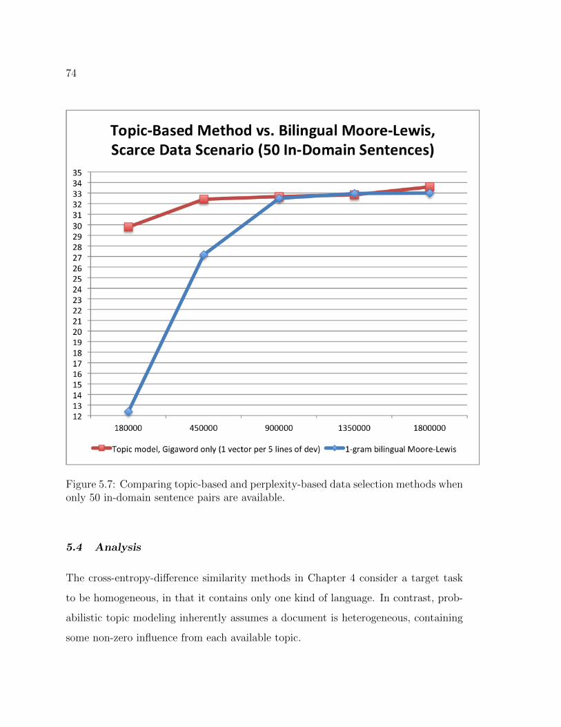
74
Figure 5.7: Comparing topic-based and perplexity-based data selection methods whenonly 50 in-domain sentence pairs are available.
5.4 Analysis
The cross-entropy-difference similarity methods in Chapter 4 consider a target task
to be homogeneous, in that it contains only one kind of language. In contrast, prob-
abilistic topic modeling inherently assumes a document is heterogeneous, containing
some non-zero influence from each available topic.

75
To quantify topical similarity relative to a target task, we still assume the target task
contains a heterogeneous mix of topics, and that each sentence in the task has its own
topic distribution vector.
Topic-based methods for data selection always substantially outperform random
selection. However, the topic-based approach is never clearly better than using cross-
entropy difference, except in very constrained scenarios with both extremely limited
training data and selecting very small amounts of relevant data to train the translation
systems. Such situations are not common.
In Section 5.3.2 we showed that the content of a talk drifts as it is delivered,
though overall the dominant topic appears in most of the talk’s sections. In the topic
heatmaps of Figures 5.1-5.3, one can see that topic 33 dominates all of the talks in
ted-1pct-dev. Each talk also has significant weights for other topics: The first talk
is also about topics 9 and 63, the second one weights 15 and 28, and the third talk
contains a good deal of topics 15 and 73. The top keywords for these secondary topics,
as automatically determined by Mallet, are listed in Table 5.6. These word clusters
have interpretable topics, perhaps: space science, personal development, political
commentary, engineering design, and British Commonwealth armed forces.
The cooccurrence of these secondary topics within a single talk is reasonable. In
the first talk, topics 9 and 63 could relate as aerospace engineering, which matches the
actual title of the talk: “The Sound the Universe Makes”, with metadata keywords
“science, universe”. Similarly, topics 15 and 28 together could indicate a personal
experience with politics, lining up with the talk’s actual title “Inge Missmahl Brings
Peace to the Minds of Afghanistan” and metadata keywords: “brain, culture, global
issues, peace, politics, potential, poverty, psychology, violence, war”. In the third talk,
topics 15 and 73 could characterize first-hand life in the military, as would be expected
in a talk titled “Inside a School for Suicide Bombers” with metadata keywords “arts,
children, culture, film, politics, war”.

76
9 space satellite systems earth csa canadian technology light radar radio mis-
sion station remote satellites science sun band field stars communications fre-
quency mhz mars observation international using technologies ground tele-
scope applications image star images high sky sensing spectrum radarsat
navigation solar mobile imaging optical flight centre instruments sensors gps
15 help us way get find good take know very like own want better life much
able experience best others often learn look different person understand give
because now right feel keep go even ways why every place things just think
family ask needs example problems become possible children then another
while come together themselves making might day without home doing
28 such however even because must often government political very fact without
power problem much against cannot now problems still way too might state
rather situation become difficult us while both own less did lack example
clear issue far view although yet case since result therefore itself thus another
indeed themselves conflict little given different point simply nor always means
63 equipment vehicle vehicles building materials such material using designed air
light design parts devices off systems construction hand side area motor must
power surface control wood mm small type fire pressure down electrical back
storage room device floor cm line maintenance then machine car machines
body colour top plastic repair clothing metal space container concrete inside
73 canadian war aircraft air during force military training soldiers wing army
forces rescue flight ship search th sar royal squadron crew british officer ships
fire battle day troops men navy number hmcs while pilot operations sea
st second commander afghanistan helicopter flying corporal exercise coast
general regiment story captain service off team members naval home ground
Table 5.6: Top keywords for secondary topics in ted-1pct-dev.

77
Topic 33, the one that is most significant to nearly all of the talks in the TED
task, is slightly different. Its keywords appear in Table 5.7. These keywords include
a number of closed-class words, possessives, adjectives, prepositions, and very few
verbs or nouns. As such, topic 33 is not about anything in particular, and so none of
the TED talks can be particularly about topic 33 either. And yet, the topic model
identifies topic 33 as being central to the TED translation task, and as being the single
most important characteristic of TED-like data. Experiment 1 supports the topic
model’s judgement: Selecting the 260k sentences from Gigaword whose dominant
topic is 33 produces SMT systems that score 2 BLEU points higher than randomly-
selected systems trained on three times as much data. As topic 33 is not about any
particular TED talk, but still characterizes all of them, then topic 33 reflects what
all TED talks are: semi-formal, spoken, first-person presentations.
33 apos s t my me like know re just don very us now because get here think
going go ve want back then m say am way really much things good right
said let lot something look today come even take why did ll little got great
last down doing every around day thing never him life few tell put says done
always still thank too actually give find again ago off didn kind she long next
Table 5.7: Top keywords for the primary topic in ted-1pct-dev.
These topic-based experiments thus unexpectedly show that the topic of a corpus
is useful, but less so than the style of the language it contains. That is, the style of
the TED talks is the most important characteristic of the task, and not their content.
Style is reflected in word choice, among other things, and both the topic-based and
the perplexity-based methods are capturing those lexical characteristics. The results
in this chapter show that a language model is slightly better than a topic model at
doing so, and we now explore the possibility of measuring stylistic similarity directly.
78
Chapter 6
STYLE
The experiments in Chapter 4 showed that an n-gram based approach to quan-
tifying textual similarity is an effective way of identifying domain-relevant data. We
hypothesized in Chapter 5 that this improvement was largely driven by the content
words in the corpus. We found that a topic model can usefully select task-relevant
data from a general corpus, but that topic adaptation is less effective than word
n-gram cross-entropy domain adaptation. Topic-based methods seek to operate on
features that are independent of the speaker and context, and focus on content words.
However, examining the topic vectors for the TED data showed that the dominant
topic did not fit an intuitive notion of topic, but rather consisted of words associated
with an informal public speaking style. The content words alone do not suffice to
capture the most important characteristics of a corpus; the way in which the content
words are assembled into a sentence and the words used to glue them together must
also be taken into account. Instead of accidentally correlating these stylistic cues with
a topic model, we now work directly with lightweight structural features of the text.
We are interested in the underlying structures in sentences, so we prefer
linguistically-motivated classes as features. In particular, we use POS tags, as taggers
are available - and reliable - for many languages. These tags (e.g. verb, noun, deter-
miner) are often the pre-terminal nodes in a parse tree, and so they are a lightweight
representation of the syntactic structure of a sentence and thus a quantifiable proxy for
style. We refer to language models trained only on part-of-speech class sequences as
“POS LMs” for brevity, with “LM” or “lexical LM” used for the word-based models.
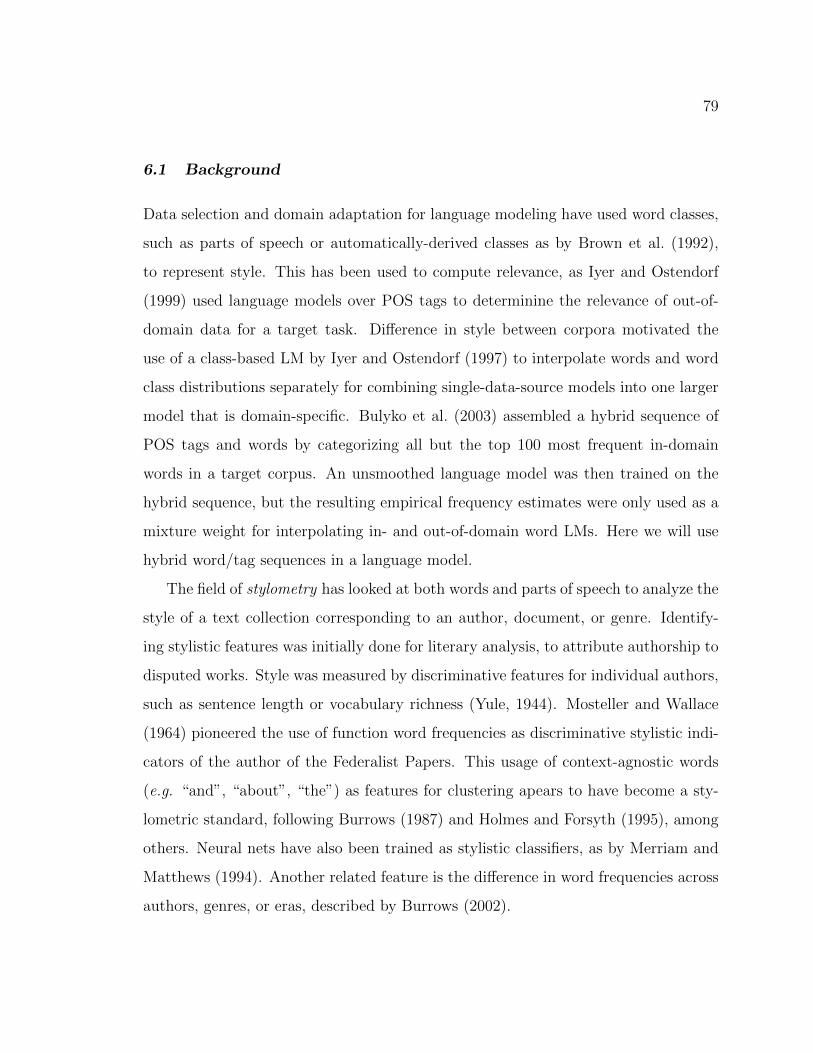
79
6.1 Background
Data selection and domain adaptation for language modeling have used word classes,
such as parts of speech or automatically-derived classes as by Brown et al. (1992),
to represent style. This has been used to compute relevance, as Iyer and Ostendorf
(1999) used language models over POS tags to determinine the relevance of out-of-
domain data for a target task. Difference in style between corpora motivated the
use of a class-based LM by Iyer and Ostendorf (1997) to interpolate words and word
class distributions separately for combining single-data-source models into one larger
model that is domain-specific. Bulyko et al. (2003) assembled a hybrid sequence of
POS tags and words by categorizing all but the top 100 most frequent in-domain
words in a target corpus. An unsmoothed language model was then trained on the
hybrid sequence, but the resulting empirical frequency estimates were only used as a
mixture weight for interpolating in- and out-of-domain word LMs. Here we will use
hybrid word/tag sequences in a language model.
The field of stylometry has looked at both words and parts of speech to analyze the
style of a text collection corresponding to an author, document, or genre. Identify-
ing stylistic features was initially done for literary analysis, to attribute authorship to
disputed works. Style was measured by discriminative features for individual authors,
such as sentence length or vocabulary richness (Yule, 1944). Mosteller and Wallace
(1964) pioneered the use of function word frequencies as discriminative stylistic indi-
cators of the author of the Federalist Papers. This usage of context-agnostic words
(e.g. “and”, “about”, “the”) as features for clustering apears to have become a sty-
lometric standard, following Burrows (1987) and Holmes and Forsyth (1995), among
others. Neural nets have also been trained as stylistic classifiers, as by Merriam and
Matthews (1994). Another related feature is the difference in word frequencies across
authors, genres, or eras, described by Burrows (2002).

80
The above-mentioned works have all used lexical (or lexically-derived) features.
Syntactic structure – or at least certain syntactic constructions – are a potentially
more informative source of stylometric features (Biber, 1988), (Baayen et al., 1996).
POS tag sequences were introduced as stylometric features by (Argamon et al., 1998),
under the guise of “pseudo-syntactic features” for document classification. Their
features were a list of 500 function words and the 685 POS trigrams that appeared in
25-75% of their training documents. Combining the two feature sets into one sparse
vector was most effective for training a classifier. Subsequent work in (Koppel et al.,
2003) used an automatic entropy-based way to measure the extent to which a word
is a stylistic indicator. They noted that the frequency of the word should be taken
into account, else the classifier learns too much about rare events whose empirical
estimates of counts and contexts might be incomplete. Sesquipedalian phrasings such
as “cunctation does not forestall the ineluctable” could be a stylistic indicator, but
might need meta-features – indicating vocabulary coverage or rarity – rather than
lexical ones. However, as pointed out in (Santini, 2004), many of those syntactic
features are just based on word identification.
Thus far the POS tag and word n-gram probabilities have been computed sepa-
rately and then combined in the overall model for style-based purposes. This moti-
vates our work, which explores both words and parts of speech, focusing on the dis-
criminative elements of each. Wx e use these newly-identified corpus differences with
the cross-entropy difference framework and bilingual scoring methods from Chapter
4 to select training data.
In summary, there is a long history of quantifying textual style, both for attribution
and for language modeling. The first task is discriminative: the goal is to partition
a vector space and correctly identify the author label of an unseen document. This
is generally accomplished by constructing a large set of textual features and then
training a classifier on the feature vectors. Style for language modeling is a sequence

81
modeling problem, where the goal is to either predict the next element in the sequence,
or provide a likelihood for the sequence.
Our work combines both the problem of sequence modeling and discrimination,
but differs from related work in that it focuses on quantifying the difference between
texts to measure relevance. Style-based models are used to measure this difference,
for the purpose of computing some score between the previously-seen sentences in
the pool and the ones in the task corpora. We explore different methods of using
lightweight syntactic information (in the form of part-of-speech tags) in combination
with words to measure the stylistic relevance of each sentence in the data pool to the
target translation task, finding that it is useful to lexicalize discriminative words.
6.2 Methods
We used the Stanford Part-of-Speech Tagger (Toutanova et al., 2003) to produce the
POS sequences for both the English and French sides of the TED and Gigaword
corpora. The English tagger uses a set of 43 tags from the Penn Treebank, and makes
distinctions such as four kinds of nouns and six kinds of verbs. The French tagger
uses 13 tags from the French Treebank, and as such only categorizes words into coarse
classes like N for all nouns, and V for all verbs.
The stylistic experiments use language models over syntactic tokens, and so we
used language modeling parameters similar to the lexical cross-entropy based selection
experiments in Chapter 4. The POS language models and hybrid word-and-POS LMs
were interpolated 4-gram models with Witten-Bell smoothing (Witten and Bell, 1991),
trained with the SRILM toolkit. Modified Kneser-Ney smoothing could not be used
because n-gram models over POS tags were not sparse enough to be able to estimate
the smoothing parameters.
All of the methods introduced in this chapter replace some of the words in the
corpora with their part-of-speech tag. These hybrid representations are used only
for the process of computing the relevance of each sentence to the task. A hybrid

82
sequence of words and POS tags can be constructed by replacing some words in a
sentence with their POS tags (categorizing some elements of the sequence). One could
equivalently start with the POS tag sequence for a sentence and put some of the words
back in (lexicalizing some elements). After all the sentences have been scored and
ranked, the original sentences (word sequences) are re-inserted, and it is these fully-
lexicalized sentences that are selected and used as training data. After scoring the
sentence pairs in the data pool using each of the methods in this chapter, we selected
the top k sentences, varying k from 180,000 to 1,800,000 sentence pairs. We trained
both a language model and an SMT system on each selected data slice, and report
perplexity scores for the LM on the task training corpus (TED-98pct-train) as well
as the usual BLEU scores on test data for each translation system.
6.3 POS Tag Analysis
We first compared the POS tag distributions between the task (TED) and pool (Gi-
gaword) corpora. The tag set used by the Stanford Tagger for English is relatively
rich, allowing relatively fine-grained syntactic comparisons between the corpora. Fig-
ure 6.1 shows the empirical frequency of each English POS tag in the TED corpus
(x axis) and Gigaword (y axis). We can measure how discriminative each English
POS tag is by computing how far each tag’s point in Figure 6.1 is from the blue line
representing equiprobability. A POS tag that is close to the diagonal line, like DT,
has little difference between its empirical frequencies in TED and Gigaword. Tags
above the line, like NNS, appear more often in Gigaword. Tags below the line, such as
RB, are more common in TED. Figure 6.2 shows the resulting distance and polarity
for each of the 43 English POS tags. Nine parts of speech are substantially more
common in one corpus than the other, and are described in Table 6.1.
The difference between the POS tag distributions indicates a stylistic mismatch
between the task and the pool corpora. Of the 43 English tags, 9 have fairly skewed
empirical frequencies, and these 9 tags cover 45% of the tokens in the task corpus.

83
Figure 6.1: Empirical frequencies of English Part of Speech tags in the TED andGigaword corpora.
This motivates the examination of discriminative POS tags – and by extension, words
– to identify task-relevant data.

84
Figure 6.2: Distance from each English POS tag to the line of equiprobability.
POS TED % Tag Description
NN 13.5 Noun, singular or mass.
NNS 4.6 Noun, plural
JJ 5.6 Adjective (not comparative nor superlative)
CD 1.4 Cardinal number
PRP 7.4 Pronoun, personal
RB 5.4 Adverb (neither comparative nor superlative)
VBP 3.7 Verb, non-3rd person singular present
, 5.8 Punctuation mark ( , )
. 5.5 Punctuation mark, sentence closer ( . ; ? *)
Table 6.1: English POS tags with biased empirical distributions towards either TEDor Gigaword.

85
6.4 Experiments
6.4.0 Baseline: Random Selection
We use the same baseline as Experiments 4.4 and 5.3.0. Having shuffled the sentences
in the pool corpus, we built SMT systems - labeled as random - on subsets of increasing
size. We also compare against the historical baseline in Chapter 4, labeled as lexical
perplexity-based filtering. Finally, we can compare against the new methods
from Chapter 4, as either monolingual (in English, the input side) or bilingual lexical
cross-entropy difference.
6.4.1 Experiment: Selecting Text with POS Language Models
We replaced all the words in the task and pool corpora with their POS tags, and
trained 4-gram POS language models over each corpus’ tag sequences. The perplexity-
based and cross-entropy-difference selection methods from Chapter 4 were then ap-
plied, using the POS LMs instead of word-based models. After sorting the (fully
lexicalized) sentences by their POS-based selection scores, we selected the top k and
trained lexical language models on the sentences. Table 6.2 contains their perplex-
ity scores on TED-98pct-train. The cross-entropy difference method from Moore
and Lewis (2010) described in Chapter 4 provides a substantial improvement over
the perplexity-based filtering, halving the perplexity of the selected language mod-
els. This is expected, as the word-only model more accurately captures the objective
and the evaluation metric. However, the performance gap between the POS-only and
word-only models with cross-entropy difference is unexpectedly small. Increasing the
order of the POS n-gram models to 6 or 8 does not provide any improvements over
the 4-gram POS models.
We trained SMT systems on the subsets, and show their BLEU scores on ted-1pct-
test in Table 6.3. The perplexity-based filtering method lags significantly behind the
cross-entropy difference method, particularly for the POS-only models confirming the
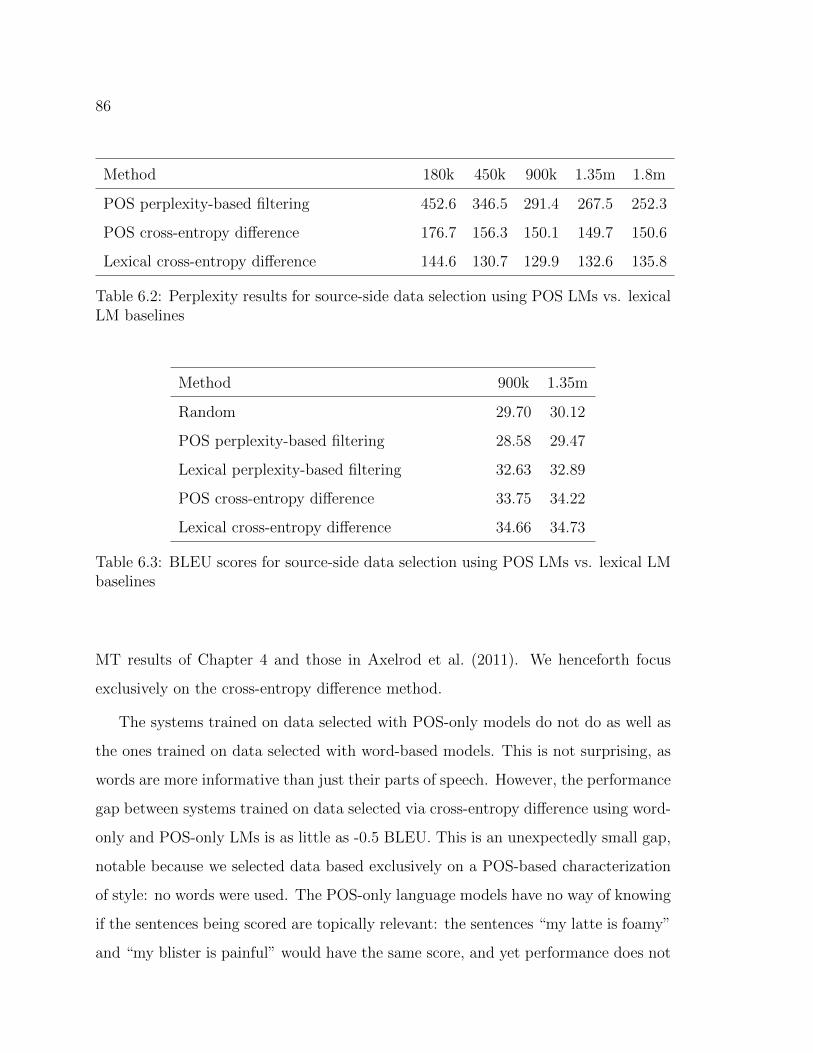
86
Method 180k 450k 900k 1.35m 1.8m
POS perplexity-based filtering 452.6 346.5 291.4 267.5 252.3
POS cross-entropy difference 176.7 156.3 150.1 149.7 150.6
Lexical cross-entropy difference 144.6 130.7 129.9 132.6 135.8
Table 6.2: Perplexity results for source-side data selection using POS LMs vs. lexicalLM baselines
Method 900k 1.35m
Random 29.70 30.12
POS perplexity-based filtering 28.58 29.47
Lexical perplexity-based filtering 32.63 32.89
POS cross-entropy difference 33.75 34.22
Lexical cross-entropy difference 34.66 34.73
Table 6.3: BLEU scores for source-side data selection using POS LMs vs. lexical LMbaselines
MT results of Chapter 4 and those in Axelrod et al. (2011). We henceforth focus
exclusively on the cross-entropy difference method.
The systems trained on data selected with POS-only models do not do as well as
the ones trained on data selected with word-based models. This is not surprising, as
words are more informative than just their parts of speech. However, the performance
gap between systems trained on data selected via cross-entropy difference using word-
only and POS-only LMs is as little as -0.5 BLEU. This is an unexpectedly small gap,
notable because we selected data based exclusively on a POS-based characterization
of style: no words were used. The POS-only language models have no way of knowing
if the sentences being scored are topically relevant: the sentences “my latte is foamy”
and “my blister is painful” would have the same score, and yet performance does not

87
plummet. This shows that the structural characteristics of a text can be almost as
strong an indicator of relevance as using the words themselves for selection. In other
words, how sentences are phrased contains almost as much information about task
relevance as what is actually being said.
6.4.2 Experiment: Hybrid Word and POS Selection Models
The performance gap between the lexicalized and categorized versions of the selection
methods in Experiment 6.4.1 indicates that words do matter when quantifying rele-
vance. However, we wish to know whether all the words in the corpus are useful in
this regard. Starting with the POS-tag sequences for each sentence in the data pool,
we constructed a hybrid POS and word corpus by lexicalizing the tags for the top 100,
500, and 5000 most frequent words in TED-98pct-train. The language models used
for selection were trained on these corpora, making them hybrid class-and-n-gram
models. The top 100 words includes all those that appear at least 3,761 times in the
TED training corpus, the top 500 appear at least 479 times, and the top 5000 words
have a minimum count of 28. The top 100 words cover 61.8% of the TED corpus,
the top 500 cover 77.7%, and the top 5000 cover 93.6%. To verify that the changes
in perplexity and BLEU score are due to the addition of POS tags and not just due
to filtering the in-domain vocabulary, we also select data using only the top 5000
most frequent words in TED, ignoring the rest entirely. Tables 6.4 and 6.5 show the
effect of gradually incorporating more words back into the data selection models for
language modeling and SMT.
For the purpose of building task-specific language models, Table 6.4 shows it is
best not to replace any words with their part of speech tag. This result is intuitive,
as language models are evaluated using word perplexity, and all words affect the
score. Adding the top 100, then 500, and finally 5000 words produces systems that
are increasingly better than the POS-only system and thus closer in performance to
the fully lexicalized system. From this we determine that the benefit of using words

88
LM used for Cross-Entropy Difference 180k 450k 900k 1.35m 1.8m
POS 176.7 156.3 150.1 149.7 150.6
POS + top100-ted words 160.3 144.7 141.5 142.9 144.8
POS + top500-ted words 152.1 139.4 138.7 141.0 143.6
POS + top5000-ted words 142.7 132.0 132.0 134.6 137.6
Words only 144.6 130.7 129.9 132.6 135.8
Only top5000-ted words 167.0 149.0 140.4 140.1 141.4
Table 6.4: Perplexity results for source-side data selection using hybrid LMs on POStags plus the most frequent words in TED
instead of POS tags for data selection is largely due to a small number of words in the
task vocabulary. Table 6.4 also shows that perplexity increases when selecting more
than 900k sentences. The BLEU scores does not deteriorate in the same manner, so
perplexity cannot be relied upon too much as an indicator of translation performance.
LM used for Cross-Entropy Difference 900k 1.35m
Random 29.70 30.12
Part of speech 33.75 34.22
POS + top100-ted words 33.99 34.37
POS + top500-ted words 34.25 34.29
Only top5000-ted words 34.47 34.60
POS + top5000-ted words 34.92 35.10
Words only 34.66 34.73
Table 6.5: BLEU scores for source-side data selection using hybrid LMs on POS tagsplus the most frequent words in TED
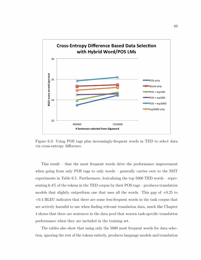
89
Figure 6.3: Using POS tags plus increasingly-frequent words in TED to select datavia cross-entropy difference.
This result – that the most frequent words drive the performance improvement
when going from only POS tags to only words – generally carries over to the SMT
experiments in Table 6.5. Furthermore, lexicalizing the top 5000 TED words – repre-
senting 6.4% of the tokens in the TED corpus by their POS tags – produces translation
models that slightly outperform one that uses all the words. This gap of +0.25 to
+0.4 BLEU indicates that there are some less-frequent words in the task corpus that
are actively harmful to use when finding relevant translation data, much like Chapter
4 shows that there are sentences in the data pool that worsen task-specific translation
performance when they are included in the training set.
The tables also show that using only the 5000 most frequent words for data selec-
tion, ignoring the rest of the tokens entirely, produces language models and translation

90
systems that are noticeably worse than when using the top 5000 words plus POS tags
for the rest of the tokens. The 5000-word-only system performs about as well as one
using only 500 words – one tenth the vocabulary – plus POS tags for the rest of
the tokens. The performance of the hybrid POS tag and top 5000-word model for
data selection is therefore not exlusively due to filtering out unhelpful words from the
vocabulary. The POS tags of the less-frequent words contain information about the
structure of the sentence, and this syntactic information is a better indicator of the
sentence’s relevance than the words themselves.
6.4.3 Experiment: Discriminative Tags for Hybrid Word and POS Selection Models
We showed in Experiment 6.4.2 an easy way to improve upon the standard approach
to data selection for machine translation. A hybrid corpus consisting of POS tags
for every word except the top 5000 TED words can be used to select more-relevant
data than using all of the words. Low-frequency words are thus less important for
computing relevance, and we focus on words with more robust empirical evidence.
We examine these most frequent words in the task corpus to better understand the
underlying reasons for the improvement. We start with only the POS tag sequences
for each corpus, and selectively lexicalize certain tags and/or words.
The POS tag analysis in Section 6.3 showed that some of the POS tags were
strongly discriminative, with empirical frequencies skewing towards either TED or
Gigaword. In this experiment, we test whether these POS tags are informative for
the purpose of computing task relevance. Of the tokens in TED-98pct-train, 61.8%
(1.7m of 2.7m) are one of the top 100 most frequent TED words. The distribution of
the top dozen POS tags for those 100 words, measured by the percentage of the tokens
in TED-98pct-train that they cover, is listed in Table 6.6. The most TED-skewed
tags (PRP/RB/VBP/quote/period) account for over 18% of the tokens covered by
the top 100 words.
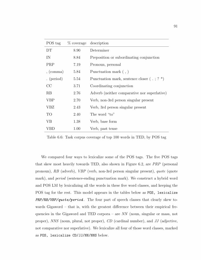
91
POS tag % coverage description
DT 8.90 Determiner
IN 8.84 Preposition or subordinating conjunction
PRP 7.19 Pronoun, personal
, (comma) 5.84 Punctuation mark ( , )
. (period) 5.54 Punctuation mark, sentence closer ( . ; ? *)
CC 3.71 Coordinating conjunction
RB 2.76 Adverb (neither comparative nor superlative)
VBP 2.70 Verb, non-3rd person singular present
VBZ 2.43 Verb, 3rd person singular present
TO 2.40 The word “to”
VB 1.38 Verb, base form
VBD 1.00 Verb, past tense
Table 6.6: Task corpus coverage of top 100 words in TED, by POS tag
We compared four ways to lexicalize some of the POS tags. The five POS tags
that skew most heavily towards TED, also shown in Figure 6.2, are PRP (personal
pronoun), RB (adverb), VBP (verb, non-3rd person singular present), quote (quote
mark), and period (sentence-ending punctuation mark). We construct a hybrid word
and POS LM by lexicalizing all the words in these five word classes, and keeping the
POS tag for the rest. This model appears in the tables below as POS, lexicalize
PRP/RB/VBP/quote/period . The four part of speech classes that clearly skew to-
wards Gigaword – that is, with the greatest difference between their empirical fre-
quencies in the Gigaword and TED corpora – are NN (noun, singular or mass, not
proper), NNS (noun, plural, not proper), CD (cardinal number), and JJ (adjective,
not comparative nor superlative). We lexicalize all four of those word classes, marked
as POS, lexicalize CD/JJ/NN/NNS below.

92
Experiment 6.4.2 suggests that it is detrimental to model all infrequent words.
With the hybrid models we have so far lexicalized either frequent words, or entire
POS classes, but not both. As such, we take the list of the top 5000 most frequent
words in TED and discard all words that have a POS tag other than CD, JJ, NN,
or NNS. While the four POS tags cover 25.3% of the TED corpus, the 3,902 words
that are both in the top 5000 most frequent TED words and are tagged with one of
those four classes cover 20.3% of the TED corpus, which is substantially less than the
93.4% covered by the full list of top 5000 words. We thus have 80% of the tokens in
the TED corpus appearing as POS tags when training the hybrid model (system POS,
lexicalize [CD/JJ/NN/NNS and in top5000-ted]). We do the same intersecting
of the Gigaword-like classes (CD/JJ/NN/NNS ) and the top5000-ted list, keeping the
intersection and using POS tags for all other words. This last system appears as POS,
lexicalize [ CD/JJ/NN/NNS and in top5000-ted ] in Tables 6.7 and 6.8.
LM used for Cross-Entropy Difference 180k 450k 900k 1.35m 1.8m
Parts-of-speech only 176.7 156.3 150.1 149.7 150.6
POS + top5000-ted words 142.7 132.0 132.0 134.6 137.6
Words only 144.6 130.7 129.9 132.6 135.8
POS, lexicalize TED-ish tags 167.0 150.4 147.2 148.5 150.4
POS, lexicalize [ TED-ish tags
and in top5000-ted ]
156.2 143.0 141.8 143.9 146.3
POS, lexicalize Gigaword-ish tags 184.1 146.6 140.0 140.5 142.4
POS, lexicalize [ Gigaword-ish tags
and in top5000-ted ]
150.2 137.7 136.5 138.6 141.0
Table 6.7: Perplexity results for source-side data selection using linguistically-motivated hybrid LMs
Table 6.7 shows that for language modeling, the words in the Gigaword-like classes

93
LM used for Cross-Entropy Difference 900k 1.35m
Random 29.70 30.12
Parts-of-speech only 33.75 34.22
POS + top5000-ted words 34.92 35.10
Words only 34.66 34.73
POS, lexicalize PRP/RB/VBP/quote/period 33.90 33.66
POS, lexicalize [ PRP/RB/VBP/quote/period
and in top5000-ted ]
33.90 34.27
POS, lexicalize CD/JJ/NN/NNS 34.05 34.48
POS, lexicalize [ CD/JJ/NN/NNS
and in top5000-ted ]
34.45 34.18
Table 6.8: BLEU scores for source-side data selection using linguistically-motivatedhybrid LMs.
(CD/JJ/NN/NNS ) are more helpful for quantifying relevance than the words in the
TED-ish classes (PRP/RB/VBP/quote/period). The words in the TED-like classes
hardly provide any improvement over the POS-only model. As these tags are indica-
tors of task relevance, it might not be necessary to lexicalize the tags in the hybrid
model. In the case of the Gigaword-like tags, they also cover a larger percentage
of the Gigaword corpus than the TED-ish tags do – by definition – and thus might
provide more information about the data to be scored. For both sets of word classes,
performance improves when restricting the words from those classes that are kept to
ones that also are in the top 5000 most frequent words. However, using all the words
in the top 5000 list is better than any of the new systems, and the fully-lexicalized
system remains best overall.
In the MT experiments in Table 6.8, the results are less clear. We saw in Exper-
iment 6.4.1 that training the selection models on POS tags only is worse than using

94
all the words. One might expect that the performance of models that lexicalize a
fraction of the words in the vocabulary would fall between the word-only and POS-
only scores. This is not the case when lexicalizing the TED-skewed word classes. By
elimination, the words in Gigaword-skewed word classes must be the important ones
to lexicalize to bridge the gap between the word-only and POS-only models. MT
performance does not degrade much when lexicalizing only the frequent words in the
POS tag clusters instead of all such words, again indicating that the frequency of the
words that are kept is important.
Taken together, the results indicated that infrequent words are not useful for com-
puting relevance, and that furthermore not all the frequent words are equally helpful.
With this in mind, we turned to examining frequent words that are discriminative.
6.4.4 Experiment: Biased Hybrid POS and Word Selection Models
In Experiment 6.4.3 we lexicalized word classes that skewed towards or away from the
task. The most improvement came from keeping word classes that biased away from
TED and towards Gigaword, whose presence indicates a lower likely relevance, yet we
also found that the frequent words in TED were the most useful. In this experiment,
we lexicalized individual words that satisfy the same criteria of being both frequent
and discriminative.
First we relaxed the inclusion criterion of being “frequent” words. We kept all
6,333 words that had a minimum count of 20 in both the TED and the Gigaword
corpora, and replaced the rest with their POS tags, listed as system POS, lexicalize
[ CountTED ≥ 20 and CountGigaword ≥ 20 ]. A similar system was built keeping
all words with a minimum count of 10 in each corpus (system POS, lexicalize
[ CountTED ≥ 10 and CountGigaword ≥ 10 ]). The results of using these hybrid
models for data selection are in Tables 6.9 and 6.10. Keeping more words decreases
the perplexity score of a language model trained on the selected data. As expected,
the perplexities of systems with increasing numbers of words converge to the score

95
of a system that uses all the words. The gap between the selected systems and the
all-words one is small. For SMT, the systems with minimum counts of 10 and 20
each matched the words-only system, confirming that performance is driven by the
frequent words in TED. The system retaining the top 5000 TED words was slightly
better overall.
Next, we applied a minimum threshold for the difference between each word’s
empirical frequencies in the two corpora. We compared differences of empirical fre-
quencies, skewed towards either corpus, of at least 10−4, 10−5, and 10−6. These retain
words with varying levels of bias, indicating probable corpus membership. The dis-
tribution of empirical frequency deltas for vocabulary words with a minimum count
of 20 in each corpus is shown in blue in Figure 6.4, with the thresholds marked in
red. Judging by the gap between 10−6 and −10−6, almost no words have an empirical
frequency delta of less than |10−6|, and few have a bias greater than |10−4|.
Figure 6.4: Empirical frequency thresholds of 10−4, 10−5, and 10−6 for vocabularywords with a minimum count of 20 in both TED and Gigaword.
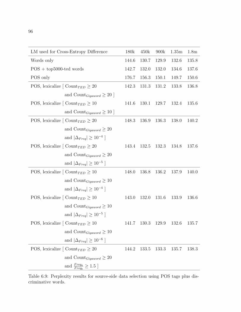
96
LM used for Cross-Entropy Difference 180k 450k 900k 1.35m 1.8m
Words only 144.6 130.7 129.9 132.6 135.8
POS + top5000-ted words 142.7 132.0 132.0 134.6 137.6
POS only 176.7 156.3 150.1 149.7 150.6
POS, lexicalize [ CountTED ≥ 20
and CountGigaword ≥ 20 ]
142.3 131.3 131.2 133.8 136.8
POS, lexicalize [ CountTED ≥ 10
and CountGigaword ≥ 10 ]
141.6 130.1 129.7 132.4 135.6
POS, lexicalize [ CountTED ≥ 20
and CountGigaword ≥ 20
and |∆Freq| ≥ 10−4 ]
148.3 136.9 136.3 138.0 140.2
POS, lexicalize [ CountTED ≥ 20
and CountGigaword ≥ 20
and |∆Freq| ≥ 10−5 ]
143.4 132.5 132.3 134.8 137.6
POS, lexicalize [ CountTED ≥ 10
and CountGigaword ≥ 10
and |∆Freq| ≥ 10−4 ]
148.0 136.8 136.2 137.9 140.0
POS, lexicalize [ CountTED ≥ 10
and CountGigaword ≥ 10
and |∆Freq| ≥ 10−5 ]
143.0 132.0 131.6 133.9 136.6
POS, lexicalize [ CountTED ≥ 10
and CountGigaword ≥ 10
and |∆Freq| ≥ 10−6 ]
141.7 130.3 129.9 132.6 135.7
POS, lexicalize [ CountTED ≥ 20
and CountGigaword ≥ 20
and FreqaFreqb
≥ 1.5 ]
144.2 133.5 133.3 135.7 138.3
Table 6.9: Perplexity results for source-side data selection using POS tags plus dis-criminative words.
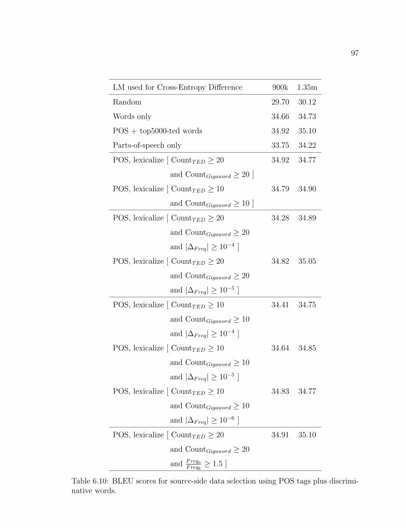
97
LM used for Cross-Entropy Difference 900k 1.35m
Random 29.70 30.12
Words only 34.66 34.73
POS + top5000-ted words 34.92 35.10
Parts-of-speech only 33.75 34.22
POS, lexicalize [ CountTED ≥ 20
and CountGigaword ≥ 20 ]
34.92 34.77
POS, lexicalize [ CountTED ≥ 10
and CountGigaword ≥ 10 ]
34.79 34.90
POS, lexicalize [ CountTED ≥ 20
and CountGigaword ≥ 20
and |∆Freq| ≥ 10−4 ]
34.28 34.89
POS, lexicalize [ CountTED ≥ 20
and CountGigaword ≥ 20
and |∆Freq| ≥ 10−5 ]
34.82 35.05
POS, lexicalize [ CountTED ≥ 10
and CountGigaword ≥ 10
and |∆Freq| ≥ 10−4 ]
34.41 34.75
POS, lexicalize [ CountTED ≥ 10
and CountGigaword ≥ 10
and |∆Freq| ≥ 10−5 ]
34.64 34.85
POS, lexicalize [ CountTED ≥ 10
and CountGigaword ≥ 10
and |∆Freq| ≥ 10−6 ]
34.83 34.77
POS, lexicalize [ CountTED ≥ 20
and CountGigaword ≥ 20
and FreqaFreqb
≥ 1.5 ]
34.91 35.10
Table 6.10: BLEU scores for source-side data selection using POS tags plus discrimi-native words.

98
The language modeling results were as expected: Using more words leads to lower
perplexities, so lower thresholds – both for counts and for bias – worked best. The
BLEU score differences in the SMT results were less clear, again highlighting the fact
that perplexity alone is not a nuanced predictor of BLEU scores. However, almost all
of the selection methods yielded systems that performed as well as the ones selected
using all of the words. The strictest frequency cutoff (10−4) was the exception, for
both words with minimum counts of 20 and of 10, as it was the experimental setting
that excluded the most words.
There are many ways we could have determined the bias of a word towards one
corpus or the other, in addition to the frequency delta used above. For example,
the ratio of the empirical frequencies could also have been used. The words with the
largest and smallest ratio of FreqTED/FreqGigaword are listed in Table 6.11. We tested
a threshold ratio of 1.5x for the empirical frequencies, whereby a word was kept only if
it had a minimum count of 20 and was at least 1.5 times more likely in one corpus than
the other (system POS, lexicalize [ CountTED ≥ 20 and CountGigaword ≥ 20 and
FreqaFreqb
≥ 1.5 ]). This system did exactly as well as the POS + top 5000 TED words
system which was the best overall SMT system. One could reasonably use these
discriminative, frequent, words instead of merely the most frequent TED words.

99
yeah 382.0
bronx 215.4
weird 205.0
tasmanian 182.1
mola 161.8
darwinian 154.1
blah 151.4
gecko 147.1
ok 145.2
feynman 141.1
[ ... ]
ensure 0.02526
4 0.02430
3 0.02079
regulations 0.02067
/ 0.01805
1 0.01442
committee 0.01298
commission 0.01279
canada 0.008380
canadian 0.004994
Table 6.11: English words with highest and lowest ratios of empirical frequency inthe TED corpus to its frequency in Gigaword.
6.4.5 Experiment: Scarce Data Scenario
As shown in Experiment 5.3.5, translation system performance can degrade signifi-
cantly in a scarce data scenario. There, a Gigaword-only topic model was decidedly

100
more useful than a unigram LM when only 50 parallel in-domain sentences were avail-
able. We now evaluate a hybrid word and POS model under similar conditions. We
suppose that there is some monolingual in-domain data – enough to determine which
are the 5000 most frequent words for the task – but only 50 parallel sentences to
use for training. These 50 in-domain sentences contain 1,173 tokens and 374 unique
words, so the monolingual in-domain data is needed to compute the in-domain empir-
ical frequencies. We construct the [ POS + top5000-ted words ] hybrid system as
in Experiment 6.4.2, but building unigram language models over the hybrid sequences
for each of Gigaword and the 50 in-domain parallel sentences due to data sparsity,
and then perform monolingual cross-entropy difference. The translation results are
in Table 6.12:
Method 180k 450k 900k 1.35m 1.8m
Topic model, Gigaword only 29.79 32.44 32.69 32.83 33.59
1-gram bilingual Moore-Lewis 12.38 27.19 32.51 32.95 33.01
POS + top5000-ted words 30.55 32.48 33.43 33.25 33.44
Table 6.12: Comparing hybrid word/POS, topic-based and perplexity-based dataselection methods when only 50 in-domain sentence pairs are available.
All of the systems do worse with only 50 parallel in-domain sentences than with
138k sentences of TED-train, as expected. The hybrid system performs the best in
this scenario, surpassing by approximately +0.75 BLEU over the method using a
topic model trained on millions of documents. The use of POS tags for infrequent
words, whose empirical counts on only 50 sentences are very likely skewed, mitigates
the sparsity problem while still retaining useful information about the sentence. The
only consideration for this method is that it requires enough monolingual in-domain
data to compute the top 5000 words. In this case we used the source side of the TED
training set, which is otherwise not used in this experiment.
101
6.4.6 Experiment: Bilingual Hybrid POS and Word Selection Models
Lastly, we examine bilingual extensions of the methods presented in this chapter.
The French part-of-speech tagger has a limited tagset, unlike the English one. As
in Experiment 6.4.1, we replaced all the words in both sides of the task and pool
corpora with their POS tags, and trained 4-gram POS language models over the tag
sequences. The gap in perplexity between the monolingual and bilingual POS-only
selection models shown in Table 6.13 is negligible. In contrast, the difference between
the word-only model scores is at least 3 perplexity points. This indicates that the
coarse French POS tag model is not as effective as the English one, as the French-side
cross-entropy difference score hardly contributes to the bilingual score. This is borne
out by the BLEU scores in Table 6.14 of SMT systems built on data selected by
POS-only models, as the bilingual models are not clearly better than the monolingual
ones. The exception is when 900k sentences are selected, and then the bilingual POS
tag selection method is +0.4 BLEU better than its monolingual equivalent.
We then performed the bilingual version of Experiment 6.4.2, keeping only the
top 5000 most frequent words in each half of the TED parallel corpus, and replacing
the rest with their POS tag. Again, the only difference between the monolingual
and bilingual versions was when selecting 900k sentences. At this subcorpus size, the
bilingual selection method very slightly outperformed the fully lexicalized bilingual
cross-entropy difference system from Chapter 4, showing the potential of the bilingual
style-based selection methods.
We also constructed the bilingual version of Experiment 6.4.4, retaining words
that had a corpus bias of at least 10−5 in either language, and using POS tags for the
rest. This bilingual experiment outperformed its monolingual counterpart, but again
did not quite improve upon the bilingual word-only selection method.

102
LM used for Cross-Entropy Difference 180k 450k 900k 1.35m 1.8m
POS only (monolingual) 176.7 156.3 150.1 149.7 150.6
POS only (bilingual) 177.9 157.0 150.5 149.8 150.8
Words only (monolingual) 144.6 130.7 129.9 132.6 135.8
Words only (bilingual) 149.7 134.6 133.5 135.9 138.9
POS + top5000-ted words (monolingual) 142.7 132.0 132.0 134.6 137.6
POS + top5000-ted words (bilingual) 145.1 134.8 134.6 137.1 139.9
POS, lexicalize [ CountTED ≥ 10
and CountGigaword ≥ 10
and |∆Freq| ≥ 10−5 ]
(monolingual)
143.0 132.0 131.6 133.9 136.6
POS, lexicalize [ CountTED ≥ 10
and CountGigaword ≥ 10
and |∆Freq| ≥ 10−5 ]
(bilingual)
145.7 135.3 134.6 136.6 139.1
Table 6.13: Perplexity results for data selection using bilingual hybrid sequences.
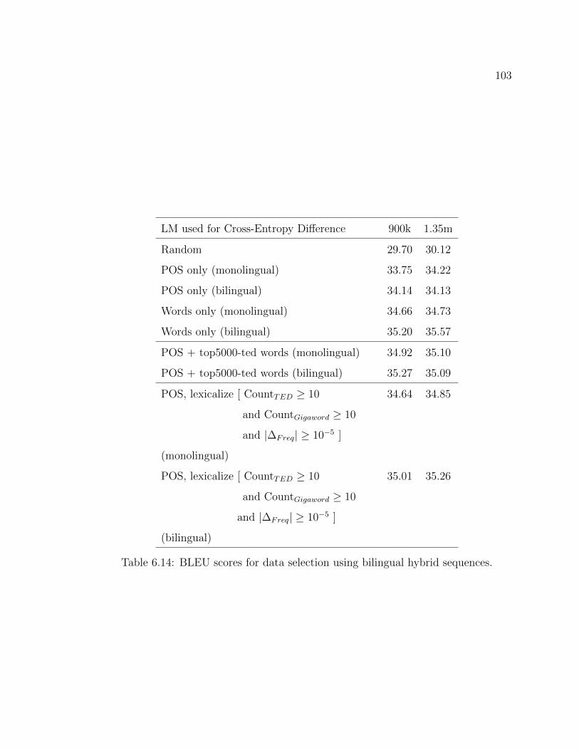
103
LM used for Cross-Entropy Difference 900k 1.35m
Random 29.70 30.12
POS only (monolingual) 33.75 34.22
POS only (bilingual) 34.14 34.13
Words only (monolingual) 34.66 34.73
Words only (bilingual) 35.20 35.57
POS + top5000-ted words (monolingual) 34.92 35.10
POS + top5000-ted words (bilingual) 35.27 35.09
POS, lexicalize [ CountTED ≥ 10
and CountGigaword ≥ 10
and |∆Freq| ≥ 10−5 ]
(monolingual)
34.64 34.85
POS, lexicalize [ CountTED ≥ 10
and CountGigaword ≥ 10
and |∆Freq| ≥ 10−5 ]
(bilingual)
35.01 35.26
Table 6.14: BLEU scores for data selection using bilingual hybrid sequences.

104
6.4.7 Summary
We see that replacing 7.1% of the words in the English side of the task and pool cor-
pora with their POS tags before training monolingual data selection models leads to
better downstream performance for both language modeling and machine translation
than using all of the words in the vocabulary. The words being replaced either are
poor differentiators between the corpora, or else are indicators of the task corpus but
appear rarely. Style alone proves to be an important component of task-specific tex-
tual relevance, and the selective integration of words into a purely structural model of
the corpus produces informative models that capture both what the corpus is about
and how it is expressed. With only a few thousand words – 8-13% of the task vocabu-
lary – it is possible to select data that is more relevant to the task, both for language
modeling and statistical machine translation, than if one considers the entire corpus
as the complete representation of the task. For each minimum count threshold, the
most biased words provide most of the system improvement, but filtering these words
according to an empirical frequency delta does not provide further improvement. A
frequency ratio threshold, however, is promising. The hybrid models also provide an
improvement when bilingual in-domain data is scarce.
Bilingual extensions of the style-based selection methods presented in this chapter
outperform their monolingual (English-side) cousins. However, the French POS tags
do not contribute as much information as the English ones, and so the bilingual POS
tag methods perform about as well as the bilingual word-only methods. We hypoth-
esize that the current French tagger is not granular enough to capture the stylistic
differences that the English-side methods do by identifying words that discriminate
between the task and the pool corpora. We conclude that style-based selection meth-
ods can outperform the current state of the art when applied to the half of a bilingual
corpus for which a robust part of speech tagger is available.

105
Chapter 7
CROSS-METHOD COMPARISONS
7.1 Using Selected Data
We showed in Chapters 4, 5 and 6 that it is possible to identify and select task-relevant
training data from a large pool. This selected data can be used to train a stand-alone,
task-specific, system with improved performance over the previous baselines. There
remains the pragmatic question as to how useful the selected data is when used in
combination with the existing in-domain data. Our previous work (Axelrod et al.,
2011) suggests best performance comes from a multi-model translation system. This
combined system, described by Koehn and Schroeder (2007), uses two phrase tables
directly in the decoder, one learned from the in-domain data and the other trained
on the selected data. System tuning is done using the phrase tables in parallel, each
receiving a separate set of weights. The multi-model system thus has more parameters
to optimize than a standard translation system. Multiple LMs can be incorporated
into the multi-model system in a similar fashion. We built systems with 2 phrase
tables and 2 LMs for each of the best-performing systems from each chapter, using
a selected data slice of 1.35M sentences for each method along with the in-domain
corpora. We also built a similar system for the random selection baseline. We used
the in-domain data to augment the following translation systems:
• Random Selection: Randomly-selected training data, used as a simple base-
line in Sections 4.4, 5.3, and 6.4.
• Bilingual cross-entropy difference: Our bilingual, SMT-specific exten-
sion from Section 4.2 of the cross-entropy difference method.
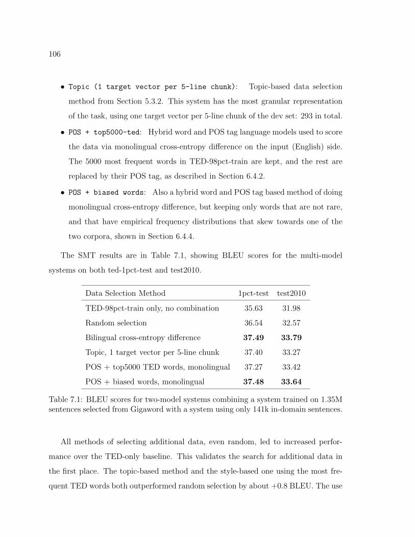
106
• Topic (1 target vector per 5-line chunk): Topic-based data selection
method from Section 5.3.2. This system has the most granular representation
of the task, using one target vector per 5-line chunk of the dev set: 293 in total.
• POS + top5000-ted: Hybrid word and POS tag language models used to score
the data via monolingual cross-entropy difference on the input (English) side.
The 5000 most frequent words in TED-98pct-train are kept, and the rest are
replaced by their POS tag, as described in Section 6.4.2.
• POS + biased words: Also a hybrid word and POS tag based method of doing
monolingual cross-entropy difference, but keeping only words that are not rare,
and that have empirical frequency distributions that skew towards one of the
two corpora, shown in Section 6.4.4.
The SMT results are in Table 7.1, showing BLEU scores for the multi-model
systems on both ted-1pct-test and test2010.
Data Selection Method 1pct-test test2010
TED-98pct-train only, no combination 35.63 31.98
Random selection 36.54 32.57
Bilingual cross-entropy difference 37.49 33.79
Topic, 1 target vector per 5-line chunk 37.40 33.27
POS + top5000 TED words, monolingual 37.27 33.42
POS + biased words, monolingual 37.48 33.64
Table 7.1: BLEU scores for two-model systems combining a system trained on 1.35Msentences selected from Gigaword with a system using only 141k in-domain sentences.
All methods of selecting additional data, even random, led to increased perfor-
mance over the TED-only baseline. This validates the search for additional data in
the first place. The topic-based method and the style-based one using the most fre-
quent TED words both outperformed random selection by about +0.8 BLEU. The use

107
of biased words in a style-based method proved a little better again, differing from the
bilingual word-only cross-entropy difference method by only some small epsilon.We
expect that given a more fine-grained French POS tagger, the bilingual style method
using POS tags and discriminative words would outperform the bilingual lexical-only
state of the art.
7.2 Interpretation
One aspect of relevant data is that it should cover as much of the task vocabulary as
possible. Table 7.2 shows how much of the TED lexicon is being found in the 900k
most relevant sentences of Gigaword.
Method (900k sentences) TED Words Coverage %
Random selection 35,043 73.5
Monolingual cross-entropy difference 37,001 77.6
Topic (1pct-dev 5lines) 37,252 78.2
POS only 34,677 72.8
POS + top5000-ted 38,372 80.5
Table 7.2: Number and coverage of the 47,661 words in the TED-98pct lexicon that areincluded in the most relevant 900k sentences according to various selection methods.
Only using POS tags captures most of the vocabulary, and it is noteworthy that the
topic-based method finds more words than lexical cross-entropy difference does. The
topic-based method selects sentences in 5-sentence chunks of about 100 words, whereas
the n-gram based method selects one sentence at a time, or about 20 words. The topic-
based methods thus reward groups of matching data rather than individual sentences,
and will rate highly any sentence full of out-of-vocabulary words if it happens to be
near enough to a small number of highly relevant sentences. By comparison, an n-
gram based model will only select out-of-vocabulary words if they are in the same

108
sentence as some task-skewed words. However, the style-based approach actually
recovered the highest number of words. This is perhaps due to preserving sentence
structure and the function of infrequent words by using their POS tags, enabling
the selection of sentences containing previously-unseen words that fill similar roles or
patterns in the task’s sentence.

109
Chapter 8
CONCLUSION
The extended SMT community includes an increasing number of multinational
firms and public entities who wish to apply SMT to practical uses, such as auto-
matically translating online knowledge bases, interacting with a linguistically diverse
customers over IM, translating large bodies of company-internal documentation for
satellite offices, or even just broadening Web presence in new markets. For these new
seats at the SMT table, data is still a gating factor for quality, but it is gated across
the dimension of task relevance. Our findings support the hypothesis that data selec-
tion needs to account for differences between the text of the task and the available
data. This thesis also contributes practicable methods for finding task-relevant data
to build machine translation systems. In short, the maxim is not just “more data is
good”, but rather “more data is good, and more data like my data is even better.”
8.1 Experimental Summary
Our work has focused on characterizing corpus differences when selecting data for
training task-oriented statistical machine translation systems. We pioneered the use
of cross-entropy difference as a data selection method in its original, monolingual
form fromMoore and Lewis (2010), and improved upon it with a bilingual extension
that improves SMT performance. Our initial work (Axelrod et al., 2011) furthermore
popularized the use of data selection for statistical machine translation, as it has
subsequently become standard practice when building task-specific machine trans-
lation systems. As confirmed in Chapter 4, the cross-entropy difference methods
substantially outperform the random selection baseline. They also provide a signifi-

110
cant improvement over the previously-standard approach, which was to use only the
in-domain data to train a language model and then use it for perplexity-based fil-
tering. In a task-specific setting, SMT benefits less from large amounts of general
content; rather, it benefits from more content in the target task, even if that content
is appreciably smaller then the available pool of data. That has become crucial as
the demand increases for application-specific machine translation.
In Chapter 5 we presented a topic-based method for data selection that centers on
inferring a topic distribution vector for the target task, and then ranking the sentences
in the data pool by the cosine similarity of their topic vectors to the target. This
extends our prior work on single-topic machine translation (Axelrod et al., 2012a),
which also treated the target task as a heterogeneous mixture of topical subcorpora,
but split the task into single-topic pieces for training and translating. Our new meth-
ods also treat the target task as a heterogenous mixture, but do not require bucketing
the data into topic-specific clusters. By using cosine distance between topic vectors,
we are able to rank the pool data by distance in the topic space, and do not need to
make any possibly-erroneous clustering decisions.
Increasingly fine-grained representations of the target task – from one topic vector
per task to one vector per TED talk, to one vector per 5-sentence chunk of text –
yield consistent improvements in downstream SMT performance. The topic model
approach also allows one to reuse a single topic model for all systems: unlike the LM-
based experiments, where the model itself represents the task, the task is represented
by its 100-dimensional vector according to some external model, or by a collection
of such vectors to capture topic dynamics. This model need not be trained on any
in-domain data at all! This allows the topic-based approach to be used in the case
where there is not enough data to train a robust n-gram language model.
Topic-based selection methods outperformed the random baseline, but were not
quite as good as the cross-entropy difference method. Examining the topic model
automatically derived from the training data showed that the most important topic

111
for the TED task was one that indicated register rather than thematic content. This
motivated our style-based approach in Chapter 6. We explored the combination of
words and POS tags to create hybrid word/class language models for computing
cross-entropy difference, instead of the strictly word-based models used in Chapter 4.
The difference in performance between using a POS class LM and using a fully
lexicalized LM for data selection appears to be due to the inclusion of discriminative
words in the model: words whose empirical frequency is much larger in one corpus
than the other. These biased words have a high overlap with the frequent words in the
corpus. They can also be broadly identified by their membership in discriminative
word classes: parts of speech whose empirical frequency is biased. Replacing non-
discriminative words with their POS tag is better than ignoring them entirely, as
the POS tags provide information about the structure of the sentence, which itself
can be indicative of both fluency and register. Overall, best results are obtained
when selecting data with cross-entropy difference using hybrid language models over
discriminative words and POS tags for non-discriminative words. A hybrid model is
extremely effective for selecting data with little in-domain parallel data, if additional
monolingual in-domain training data is available.
As a guideline for system design, if a POS tagger with a reasonably discerning
tagset is available (i.e. English treebank, 43 tags, can separate proper nouns, verb
tenses, and so on), then use the style-based method of identifying discriminative words
and replacing everything else with its POS tag. Train LMs on these hybrid represen-
tations (both task and data pool), then use cross-entropy difference as the relevance
score. If no such tagger is available, then it is best to use bilingual cross-entropy
difference over the words. The use of the topic-based methods is not recommended
except in unlikely circumstances where only dozens of parallel in-domain sentences
are available.

112
8.2 Next steps
The topic modeling method is harder and more costly to implement than the other
approaches discussed in this work. However, it cannot be dismissed entirely, as it
performs almost as well as the word-based cross-entropy method, despite the fact
that the topic model we used was only monolingual and unigram-based. Topic-based
relevance could be extended to use an n-gram topic model, and/or a multilingual one.
There are fewer tools available to do this, and they are significantly more computa-
tionally expensive, but the multi-word correlations should be more powerful than the
unigram ones that Mallet uses by default. A bilingual topic model might help by
bringing in output-side information, but a first step would be the standard trick of
concatenating the English and French sentences together and then training a regular
(monolingual) topic model. Each topic would then be expected to consist of English
words and their French translations.
The style-based method has much left to explore. Some low-hanging fruit include
a bilingual version that combines the word-based and style-based methods for parallel
corpora where there is a POS tagger for only one language. Additionally, the use of a
better French tagger might prove helpful, as well as more robust syntactic tools such
as parsers or supertaggers.
One might also wish to determine how best to build the LMs used in translation.
it is common to also build a huge language model over all available monolingual data,
to increase the fluency of the SMT output. Using three LMs could be examined: one
in-domain, one for the relevant data in pool, and one over all of the pool.
There are broader questions, as well. We have found that the style of the task
matters, and that the topic can matter, but there are surely other factors, including
other aspects of style. What else is there about a task that differentiates its language
from others, how can we quantify these features, and which of them are useful when
measuring the difference between two texts?

113
The answers will be readily applicable to the problem of data selection, of course,
but they can also have a far-ranging impact across the entire field of natural language
processing. If one could quantify the difference between two texts, then one could
also quantify the difference between two writing styles, and eventually tailor a system
to a particular person’s use of language, whether for translation, speech recognition,
or any language generation task. If one could tailor a system to a particular, fine-
grained, usage of language, then one might reasonably invert the process to create
systems whose output lacks all idiosyncrasies. This might be useful for the purpose of
maintaining anonymity, but also to generate output that is understandable by people
with a limited grasp of the language, such as children or second language learners.
One could also automatically track broad changes in style over time, perhaps from
an ethnographic perspective, and also to detect changes in one person’s own use of
language which may correlate with mood, health, as from depression or the early
onset of neurological conditions. Quantifying textual differences is one small step –
of many – towards being able to describe, perhaps even understand, one of the best
things about being human: being able to manipulate how we use our linguistic ability.
114
BIBLIOGRAPHY
Anka, P. (1969). My Way. In My Way. Reprise, 1969 edition.
Argamon, S., Koppel, M., and Avneri, G. (1998). Routing documents according to
style. Workshop on Innovative Information Systems, 60(6):581–3.
Axelrod, A. (2006). Factored Language Models for Statistical Machine Translation.
University of Edinburgh.
Axelrod, A., He, X., Deng, L., Acero, A., and Hwang, M.-Y. (2012a). New methods
and evaluation experiments on translating TED talks in the IWSLT benchmark.
ICASSP (International Conference on Acoustics, Speech, and Signal Processing).
Axelrod, A., He, X., and Gao, J. (2011). Domain Adaptation Via Pseudo In-Domain
Data Selection. EMNLP (Empirical Methods in Natural Language Processing).
Axelrod, A., Li, Q., and Lewis, W. D. (2012b). Applications of Data Selection via
Cross-Entropy Difference for Real-World Statistical Machine Translation. IWSLT
(International Workshop on Spoken Language Translation).
Baayen, H., Halteren, H. V., and Tweedie, F. (1996). Outside the cave of shad-
ows: using syntactic annotation to enhance authorship attribution. Literary and
Linguistic Computing, 11(3):121–132.
Bahl, L., Baker, J. K., Jelinek, F., and Mercer, R. L. (1977). Perplexity - A Measure
of the Difficulty of Speech Recognition Tasks. Journal of the Acoustical Society of
America, 62(Supplement 1).
115
Bahl, L., Jelinek, F., and Mercer, R. L. (1983). A Maximum Likelihood Approach
to Continuous Speech Recognition. IEEE Transactions on Pattern Analysis and
Machine Intelligence, 5(2):179–190.
Bakhtin, M. (1975). The Dialogic Imagination. University of Texas Press, Austin,
Texas.
Besling, S. and Meier, H.-G. (1995). Language Model Speaker Adaptation. Eu-
rospeech.
Biber, D. (1988). Variations Across Speech and Writing. Cambridge University Press,
Cambridge, UK.
Biber, D. (1993). Using Register-Diversified Corpora for General Language Studies.
Computational Linguistics, pages 219–241.
Birch, A., Osborne, M., and Koehn, P. (2007). CCG Supertags in Factored Statistical
Machine Translation. WMT (Workshop on Statistical Machine Translation).
Blei, D., Ng, A., and Jordan, M. (2003). Latent Dirichlet Allocation. Journal of
Machine Learning Research, 3(4-5):993–1022.
Brants, T., Popat, A. C., Xu, P., Och, F. J., and Dean, J. (2007). Large Language
Models in Machine Translation. EMNLP (Empirical Methods in Natural Language
Processing).
Brown, P. F., Cocke, J., Della Pietra, S. A., Della Pietra, V. J., Jelinek, F., Lafferty,
J. D., Mercer, R. L., and Roossin, P. S. (1990). A Statistical Approach to Machine
Translation. Computational Linguistics, 16(2):79–85.
Brown, P. F., DeSouza, P. V., Mercer, R. L., Della Pietra, V. J., and Lai, J. C.
(1992). Class-Based n-gram Models of Natural Language. Computational Linguis-
tics, 18(4):467–479.

116
Bulyko, I., Ostendorf, M., and Stolcke, A. (2003). Getting More Mileage From
Web Text Sources For Conversational Speech Language Modeling Using Class-
Dependent Mixtures. NAACL (North American Association for Computational
Linguistics).
Burrows, J. (1987). Word-Patterns and Story-Shapes: The Statistical Analysis of
Narrative Style. Literary and Linguistic Computing, 2(2):61–70.
Burrows, J. (2002). ‘Delta’: A Measure of Stylistic Difference and a Guide to Likely
Authorship. Literary and Linguistic Computing, 17(3):267 –287.
Callison-Burch, C., Koehn, P., Monz, C., Post, M., Soricut, R., and Specia, L. (2012).
Findings of the 2012 Workshop on Statistical Machine Translation. WMT (Work-
shop on Statistical Machine Translation).
Carpuat, M. and Simard, M. (2012). The Trouble with SMT Consistency. WMT
(Workshop on Statistical Machine Translation).
Cettolo, M., Girardi, C., and Federico, M. (2012). WITˆ3 : Web Inventory of Tran-
scribed and Translated Talks. EAMT (European Association for Machine Transla-
tion).
Charaudeau, P. and Maingueneau, D. (2002). Dictionnaire d’Analyse du Discours.
Le Seuil, Paris.
Chen, S. F. and Goodman, J. (1999). An Empirical Study of Smoothing Techniques
for Language Modeling. Computer Speech & Language, 13(4):359–393.
Chiang, D. (2005). A Hierarchical Phrase-Based Model for Statistical Machine Trans-
lation. ACL (Association for Computational Linguistics).
Chiang, D. (2007). Hierarchical Phrase-Based Translation. Computational Linguistics,
33(2):201–228.
117
Deerwester, S., Dumais, S. T., Furnas, G. W., Landauer, T. K., and Harshman, R.
(1990). Indexing by Latent Semantic Analysis. Journal of the American Society
for Information Science, 41:391–407.
Dempster, A. P., Laird, N. M., and Rubin, D. B. (1976). Maximum Likelihood from
Incomplete Data via the EM Algorithm. Journal of the Royal Statistical Society,
B(39):1–38.
Denkowski, M. and Lavie, A. (2011). Meteor 1.3 : Automatic Metric for Reliable
Optimization and Evaluation of Machine Translation Systems. WMT (Workshop
on Statistical Machine Translation).
Dorr, B. J. (1994). Machine Translation Divergences : A Formal Description and
Proposed Solution. ACL (Association for Computational Linguistics).
Dyer, C., Chahuneau, V., and Smith, N. A. (2013). A Simple, Fast, and Effective
Reparameterization of IBM Model 2. NAACL (North American Association for
Computational Linguistics).
Eck, M., Vogel, S., and Waibel, A. (2004). Language Model Adaptation for Statis-
tical Machine Translation based on Information Retrieval. LREC (International
Conference on Language Resources and Evaluation).
Eidelman, V., Boyd-Graber, J., and Resnik, P. (2012). Topic Models for Dynamic
Translation Model Adaptation. ACL (Association for Computational Linguistics).
Eisele, A. and Chen, Y. (2010). MultiUN : A Multilingual Corpus from United
Nation Documents. LREC (International Conference on Language Resources and
Evaluation).
Federico, M. (2002). Language Model Adaptation through Topic Decomposition and
MDA Estimation. ICASSP (International Conference on Acoustics, Speech, and
Signal Processing).

118
Federico, M., Cettolo, M., Bentivogli, L., Paul, M., and Stuker, S. (2012). Overview
of the IWSLT 2012 Evaluation Campaign. IWSLT (International Workshop on
Spoken Language Translation).
Foster, G., Goutte, C., and Kuhn, R. (2010). Discriminative Instance Weighting
for Domain Adaptation in Statistical Machine Translation. EMNLP (Empirical
Methods in Natural Language Processing).
Foster, G. and Kuhn, R. (2007). Mixture-Model Adaptation for SMT. WMT (Work-
shop on Statistical Machine Translation).
Gao, J., Goodman, J., Li, M., and Lee, K.-F. (2002). Toward a unified approach to
statistical language modeling for Chinese. ACM Transactions On Asian Language
Information Processing, 1(1):3–33.
Gasco, G., Rocha, M.-A., Sanchis-Trilles, G., Andres-Ferrer, J., and Casacuberta,
F. (2012). Does More Data Always Yield Better Translations? EACL (European
Association for Computational Linguistics).
Gildea, D. (2001). Corpus Variation and Parser Performance. EMNLP (Empirical
Methods in Natural Language Processing).
Gong, Z. and Zhou, G. (2011). Employing Topic Modeling for Statistical Machine
Translation. IEEE International Conference on Computer Science and Automation
Engineering, pages 24–28.
Halliday, M. A. K. and Hasan, R. (1976). Cohesion in English. Longman.
He, X., Axelrod, A., Deng, L., Acero, A., Hwang, M.-y., Nguyen, A., Wang, A.,
and Huang, X. (2011). The MSR System for IWSLT 2011 Evaluation. IWSLT
(International Workshop on Spoken Language Translation).

119
Heafield, K. (2011). KenLM : Faster and Smaller Language Model Queries. WMT
(Workshop on Statistical Machine Translation).
Hofmann, T. (1999). Probabilistic Latent Semantic Analysis. Uncertainty in AI.
Holmes, D. I. and Forsyth, R. S. (1995). The Federalist Revisited: New Directions in
Authorship Attribution. Literary and Linguistic Computing, 10:111 –127.
Irvine, J. (2002). Style as Distinctiveness: the Culture and Ideology of Linguistic
Differentiation. In Eckert, P. and Rickford, J. R., editors, Style and Sociolinguistic
Variation, pages 21–43. Cambridge University Press.
Iyer, R. and Ostendorf, M. (1997). Transforming Out-of-Domain Estimates to Improve
In-Domain Language Models. Eurospeech.
Iyer, R. and Ostendorf, M. (1999). Relevance Weighting for Combining Multi-Domain
data for N-gram Language Modeling. Computer Speech & Language, 13(3):267–282.
Iyer, R., Ostendorf, M., and Gish, H. (1997). Using out-of-domain data to improve
in-domain language models. IEEE Signal Processing Letters, 4(8):221–223.
Joos, M. (1961). The Five Clocks. Harcourt, Brace & World, New York.
Kessler, B., Geoffrey, N., and Schutze, H. (1997). Automatic Detection of Text Genre.
ACL (Association for Computational Linguistics).
Kiesling, S. F. (2005). Variation, Stance and Style. English World-Wide, 26(1):1–42.
Koehn, P. (2004). Statistical Significance Tests for Machine Translation Evaluation.
EMNLP (Empirical Methods in Natural Language Processing).
Koehn, P. (2005). Europarl : A Parallel Corpus for Statistical Machine Translation.
MT Summit.

120
Koehn, P., Axelrod, A., Mayne, A. B., Callison-burch, C., Osborne, M., Talbot,
D., and White, M. (2005). Edinburgh System Description for the 2005 NIST MT
Evaluation. (3):3–5.
Koehn, P., Birch, A., Callison-Burch, C., Federico, M., Bertoldi, N., Cowan, B.,
Moran, C., Dyer, C., Constantin, A., and Herbst, E. (2007). Moses: Open Source
Toolkit for Statistical Machine Translation. ACL (Association for Computational
Linguistics) Interactive Poster and Demonstration Sessions.
Koehn, P. and Haddow, B. (2012). Towards Effective Use of Training Data in Statis-
tical Machine Translation. WMT (Workshop on Statistical Machine Translation).
Koehn, P. and Monz, C. (2006). Manual and Automatic Evaluation of Machine
Translation between European Languages. WMT (Workshop on Statistical Machine
Translation).
Koehn, P., Och, F. J., and Marcu, D. (2003). Statistical Phrase-Based Translation.
NAACL (North American Association for Computational Linguistics).
Koehn, P. and Schroeder, J. (2007). Experiments in Domain Adaptation for Statistical
Machine Translation. WMT (Workshop on Statistical Machine Translation).
Koppel, M., Akiva, N., and Dagan, I. (2003). A Corpus-Independent Feature Set for
Style-Based Text Categorization. IJCAI Workshop on Computational Approaches
to Style Analysis and Synthesis.
Koppel, M. and Schler, J. (2003). Exploiting Stylistic Idiosyncrasies for Authorship
Attribution. In IJCAI’03 Workshop on Computational Approaches to Style Analysis
and Synthesis, pages 69–72.
Labov, W. (1984). Field Methods of the Project on Linguistic Change and Variation.
In Baugh, J. and Sherzer, J., editors, Language in Use, pages 28–53. Prentice Hall,
Englewood Cliffs.

121
Lopez, A. (2008). Statistical Machine Translation. ACM Computing Surveys, 40(3):1–
49.
Lu, Y., Huang, J., and Liu, Q. (2007). Improving Statistical Machine Translation
Performance by Training Data Selection and Optimization. EMNLP (Empirical
Methods in Natural Language Processing).
Mansour, S., Wuebker, J., and Ney, H. (2011). Combining Translation and Language
Model Scoring for Domain-Specific Data Filtering. IWSLT (International Workshop
on Spoken Language Translation).
Matsoukas, S., Rosti, A.-V. I., and Zhang, B. (2009). Discriminative Corpus Weight
Estimation for Machine Translation. EMNLP (Empirical Methods in Natural Lan-
guage Processing).
Merriam, T. V. N. and Matthews, R. A. J. (1994). Neural Computation in Stylom-
etry II: An Application to the Works of Shakespeare and Marlowe. Literary and
Linguistic Computing, 9:1 –6.
Mimno, D., Wallach, H. M., Naradowsky, J., Smith, D. A., and Mccallum, A. (2009).
Polylingual Topic Models. EMNLP (Empirical Methods in Natural Language Pro-
cessing).
Moore, R. and Lewis, W. (2010). Intelligent Selection of Language Model Training
Data. ACL (Association for Computational Linguistics).
Mosteller, F. and Wallace, D. L. (1964). Inference and disputed authorship: The
Federalist. Springer.
Och, F. J. (2003). Minimum Error Rate Training in Statistical Machine Translation.
ACL (Association for Computational Linguistics).

122
Och, F. J. and Ney, H. (2002). Discriminative Training and Maximum Entropy
Models for Statistical Machine Translation. ACL (Association for Computational
Linguistics).
Och, F. J. and Ney, H. (2003). A Systematic Comparison of Various Statistical
Alignment Models. Computational Linguistics, 29(1):19–51.
Papineni, K., Roukos, S., Ward, T., and Zhu, W.-j. (2002). BLEU: a method for
automatic evaluation of machine translation. ACL (Association for Computational
Linguistics).
Paul, M., Federico, M., and Stuker, S. (2010). Overview of the IWSLT 2010 Evaluation
Campaign. IWSLT (International Workshop on Spoken Language Translation),
pages 3–27.
Plank, B. and van Noord, G. (2011). Effective Measures of Domain Similarity for
Parsing. ACL (Association for Computational Linguistics).
Reid, T. B. W. (1956). Linguistics, Structuralism, Philology. Archivum Linguisticum,
8:28–37.
Riezler, S. and Maxwell III, J. T. (2005). On Some Pitfalls in Automatic Evalua-
tion and Significance Testing for MT. ACL Workshop on Intrinsic and Extrinsic
Evaluation Measures for Machine Translation and Summarization, (June).
Rosenfeld, R. (2000). Two Decades of Statistical Language Modeling: Where Do We
Go from Here? Proceedings of the IEEE, 88(8):1270–1278.
Rousseau, A. (2013). XenC : An Open-Source Tool for Data Selection in Natural
Language Processing. Prague Bulletin of Mathematical Linguistics, 100:73–82.
Ruiz, N. and Federico, M. (2011). Topic Adaptation for Lecture Translation through

123
Bilingual Latent Semantic Models. WMT (Workshop on Statistical Machine Trans-
lation).
Santini, M. (2004). A Shallow Approach To Syntactic Feature Extraction For Genre
Classification. In Proceedings of the 7th Annual Colloquium for the UK Special
Interest Group for Computational Linguistics. ITRI, University of Brighton.
Snover, M., Madnani, N., Dorr, B. J., and Schwartz, R. (2009). Fluency, Adequacy, or
HTER? Exploring Different Human Judgments with a Tunable MT Metric. WMT
(Workshop on Statistical Machine Translation).
Steyvers, M. and Griffiths, T. (2007). Probabilistic Topic Models. In Landauer, T.,
McNamara, D., Dennis, S., and Kintsch, W., editors, Latent Semantic Analysis: A
Road to Meaning. Laurence Erlbaum.
Stolcke, A. (2002). SRILM — An Extensible Language Modeling Toolkit. Interspeech.
Tam, Y.-C., Lane, I., and Schultz, T. (2007). Bilingual LSA-based adaptation for
statistical machine translation. Machine Translation, 21(4):187–207.
Tam, Y.-C. and Schultz, T. (2005). Dynamic Language Model Adaptation using
Variational Bayes Inference. Interspeech.
Tennyson, L. A. (1842). Ulysses. In Poems.
Tiedemann, J. (2009). Translating Questions for Cross-Lingual QA. EAMT (European
Association for Machine Translation).
Toutanova, K., Klein, D., Manning, C. D., and Singer, Y. (2003). Feature-Rich Part-
of-Speech Tagging with a Cyclic Dependency Network. NAACL (North American
Association for Computational Linguistics).

124
Vilar, D., Xu, J., D’Haro, L. F., and Ney, H. (2006). Error Analysis of Statisti-
cal Machine Translation Output. LREC (International Conference on Language
Resources and Evaluation).
Webber, B. (2009). Genre distinctions for Discourse in the Penn TreeBank. ACL
(Association for Computational Linguistics).
Wetzel, D. and Bond, F. (2012). Enriching Parallel Corpora for Statistical Machine
Translation with Semantic Negation Rephrasing. SSST (Workshop on Syntax, Se-
mantics, and Structure in Statistical Translation).
Witten, I. H. and Bell, T. C. (1991). The Zero-Frequency Problem: Estimating the
Probabilities of Novel Events in Adaptive Text Compression. IEEE Transactions
on Information Theory, 37(4):1085–1094.
Yasuda, K., Zhang, R., Yamamoto, H., and Sumita, E. (2008). Method of selecting
training data to build a compact and efficient translation model. IJCNLP (Inter-
national Joint Conference on Natural Language Processing).
Yule, G. U. (1944). The Statistical Study of Literary Vocabulary. Cambridge Univer-
sity Press, Cambridge, UK.