THREE ESSAYS ON INTERNATIONAL TRADE

By

Yih-ming Lin

Dissertation

Submitted to the Faculty of the

Graduate School of Vanderbilt University

in partial fulfillment of the requirements

for the degree of

DOCTOR OF PHILOSOPHY

in

Economics

August, 2005

Nashville, Tennessee

Approved:

Professor Eric W. Bond

Professor Jennifer F. Reinganum

Professor Benjamin C. Zissimos

Professor Mikhael Shor

To

My Parents and Hung-Pin

ii

ACKNOWLEDGEMENTS

I am especially indebted to my advisor, Dr. Eric W. Bond. Without his direction, suggestions and

comments, this dissertation would not have been possibly completed. I also would like to put in record my

thanks and gratitude for my committee members: Dr. Jennifer F. Reinganum, Dr. Benjamin C. Zissimos,

and Dr. Mikhael Shor for their generosity, time, and comments. They made me notice my mistakes and give

me useful suggestions. I am thankful to my wife, Hung-pin, who took care of our family when I was away.

iii

TABLE OF CONTENTS

Page

ACKNOWLEDGEMENTS …………………………………………………………………............................... iii

LIST OF TABLES ……………………………………………………................................……………………. v

LIST OF FIGURES……………………………..............................……………………………………….……. vi

Chapter

I. INTRODUCTION.............................................………………………………………………… 1 Essay 1: Bilateral trade flows and nontraded goods ………………………..............…….… 1

Essay 2: Arbitrage and the harmonization of patent lives …………………….......................1 Essay 3: Why does the U.S. prevent parallel import?.………...………….…….................... 2

II BILATERAL TRADE FLOWS AND NONTRADED GOODS ……………………………................ 3 Introduction …………………………..................................….…............................. 3 The model ………......................................................................................... 6 Data …………………………….…......................................................................... 10 Empirical results ……………....................................…………............................ 10 Conclusions .………...………….……................................................................ 12 Appendix …………………………….….................................................................. 13 References ………………………........................................................................ 15 III ARBITRAGE AND THE HARMONIZATION OF PATENT LIVES ....………...................... 17 Introduction ………………..............................................................…………….… 17 The model ………………………........................................................................ 19 The non-cooperative equilibrium…………………………….….................................... 24 Efficient international agreement ……………………….......................................... 32 Conclusions .………...………….……................................................................ 34 Appendix …………………………….….................................................................. 35 References ………………………........................................................................ 41

IV WHY DOES THE U.S. PREVENT PARALLEL IMPORTS? ……………………......………...........43 Introduction …………………………….…............................................................... 43 The single product case ………………………...................................................... 46 The welfare effects of parallel trade incorporated with innovation……………….… 48 Conclusions .………...………….……................................................................ 53 References ……………….......................................................................……… 56

iv

LIST OF TABLES Table Page II.1. 1-Si, Export/GDP Ratio (%), and Import/GDP Ratio (%) (1995)................................................................. 4 II.2. An Example with Three Countries ........................................................................................................... 8 II.3. Estimation Results................................................................................................................................. 12 IV.1. Summary of IPRs Exhaustion Regime .................................................................................................. 45

v

LIST OF FIGURES Figure Page III.1.Profit, π(λ), consumer's surplus, s(λ) and social deadweight loss, ∆(λ) ............................................ 23 III.2. Marginal benefit and marginal cost of increasing enforcement level, λ ............................................ 27 III.3. Right hand side (RHS) and left hand side (LHS) of equation (16) where λ'> λ................................. 29 III.4. The conditional best response function of the North and South ....................................................... 36 IV.1. Relative welfare, γ=5......................................................................................................................... 51 IV.2. Relative welfare, γ=10/11.................................................................................................................. 52 IV.3. The relation between elasticity of innovation, γ and x .................................................................... 54

vi

CHAPTER I

INTRODUCTION

This dissertation contains three essays. In the first essay, I consider nontraded goods as an impor-

tant impact on bilateral trade flows. A testable gravity equation is derived and a simple example

is demonstrated. In my second essay, I study a North/South model of intellectual property rights

protection in which markets are not completely segmented and investigate how arbitrage affects

IPR protection. In the third essay, we propose a two-country model of parallel trade with innova-

tion. This model tries to explain why some countries, such as the U.S., do not allow parallel trade

and some, such as Japan, do. The abstracts of these three essays are as follows:

Essay 1: Bilateral Trade Flows and Nontraded Goods

This essay develops a monopolistic competition model with nontraded goods, which provides an

explanation for why the real volume of trade is much lower than predicted by Helpman and

Krugman’s (1985) model. Furthermore, it explains the phenomenon that the volume of trade

among high-income countries is relatively larger than the volume of trade between high-income

and low-income countries. We also derive a testable gravity equation from this model. A sample

of 1995 including 118 countries is examined. Our results show that evidence from the data is

consistent with the prediction of this model; further, the goodness-of-fit increases as nontraded

goods are considered.

Essay 2: Arbitrage and the Harmonization of Patent Lives

We study a North/South model of intellectual property rights protection in which markets are not

completely segmented. We examine how the existence of arbitrage affects the incentives of countries

to set the length of patent protection. The results show that the North will not have an incentive

to completely eliminate arbitrage after patents expire in the South, even when enforcement is

costless. The results also show that, if the demand function for an innovation is linear, there exists

1

a pure-strategy Nash equilibrium of a non-cooperative game between the North and the South.

Furthermore, we demonstrate that the uniform universal standard for IPRs protection will never

achieve global Pareto efficiency when the markets are not perfectly segmented.

Essay 3: Why Does the U.S. Prevent Parallel Imports?

In this eaasy, we propose a two-country model of parallel trade with innovation. This model tries

to explain why some countries, such as the U.S., do not allow parallel imports and some, such

as Japan, do. We find that the welfare effects of parallel trade are related to the elasticity of

innovation. If the elasticity of innovation is high, the welfare of the importing country improves

when the difference between the importing and exporting markets is small, but it becomes worse

when the difference is large. Furthermore, global welfare decreases anyway when innovation is

considered. For the case of low elasticity of innovation, it is possible for global welfare to be

improved by allowing parallel trade.

2

CHAPTER II

BILATERAL TRADE FLOWS AND NONTRADED GOODS

Introduction

In the last few decades, the most important development in the theory of international trade is

the monopolistic competition model. Helpman and Krugman (1985) proposed a model in which

monopolistically competitive firms produce differentiated goods using an increasing returns to

scale technology (IRS) and all individuals have identical homothetic preferences and a “love for

variety”.1 Their model provides an explanation for the phenomenon of large volumes of trade

among similar countries with a factor-proportions view of intersectoral trade flows, which could

not be explained by the traditional Heckscher-Ohlin (HO) theorem.

In Helpman and Krugman’s model, it is assumed that the economy has free trade, balanced

trade, no transport cost, all tradeable goods, and identical production technology across countries.

The monopolistic competition model yields the following equation to predict the volume of bilateral

trade,

Mij =YiYj

Yw

= sjYi, (1)

where Mij is the imports of country i from country j, Yi(Yj) is the gross domestic product (GDP)

of country i(j), Yw is the total world income, and sj = Yj

Ywis the share of country j in total world

income. Equation (1) means that the bilateral trade flows are positively related to the product of

countries’ GDPs, which is the simplest form of gravity equation.

However, the volume of trade in the real world is much less than the amount predicted by

equation (1). For example, the volume of trade in the world is about 5,214 billion U.S. dollars,

which is much lower than the predicted number, 25,033 billion US dollars in 1995.2 Furthermore,

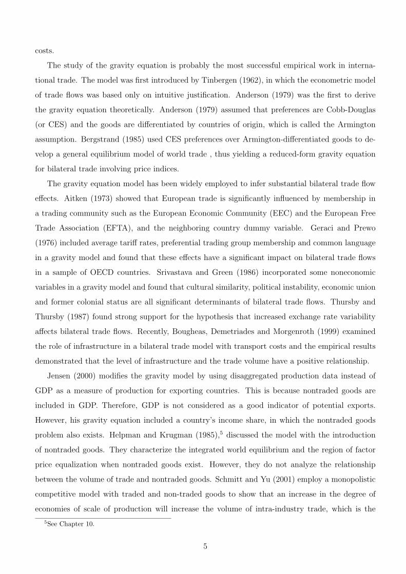
let us take a look at the country’s data. The Export/GDP ratio and Import/GDP ratio of a

sample of countries are shown in Table 1.3 The predicted Export/GDP ratio or Import/GDP ratio

1The term “love for variety ” is from Jensen (2000).2The trade data is from the CD-ROM “World Trade Flows, 1980-1997, with Production and Tariff Data,” the

predicted value is calculated based on the GDP data from World Development Indicators CD-ROM, 2000.3This is the same sample employed in Jensen (2000). This sample includes ten rich countries, ten middle income

countries, and ten poor countries.

3

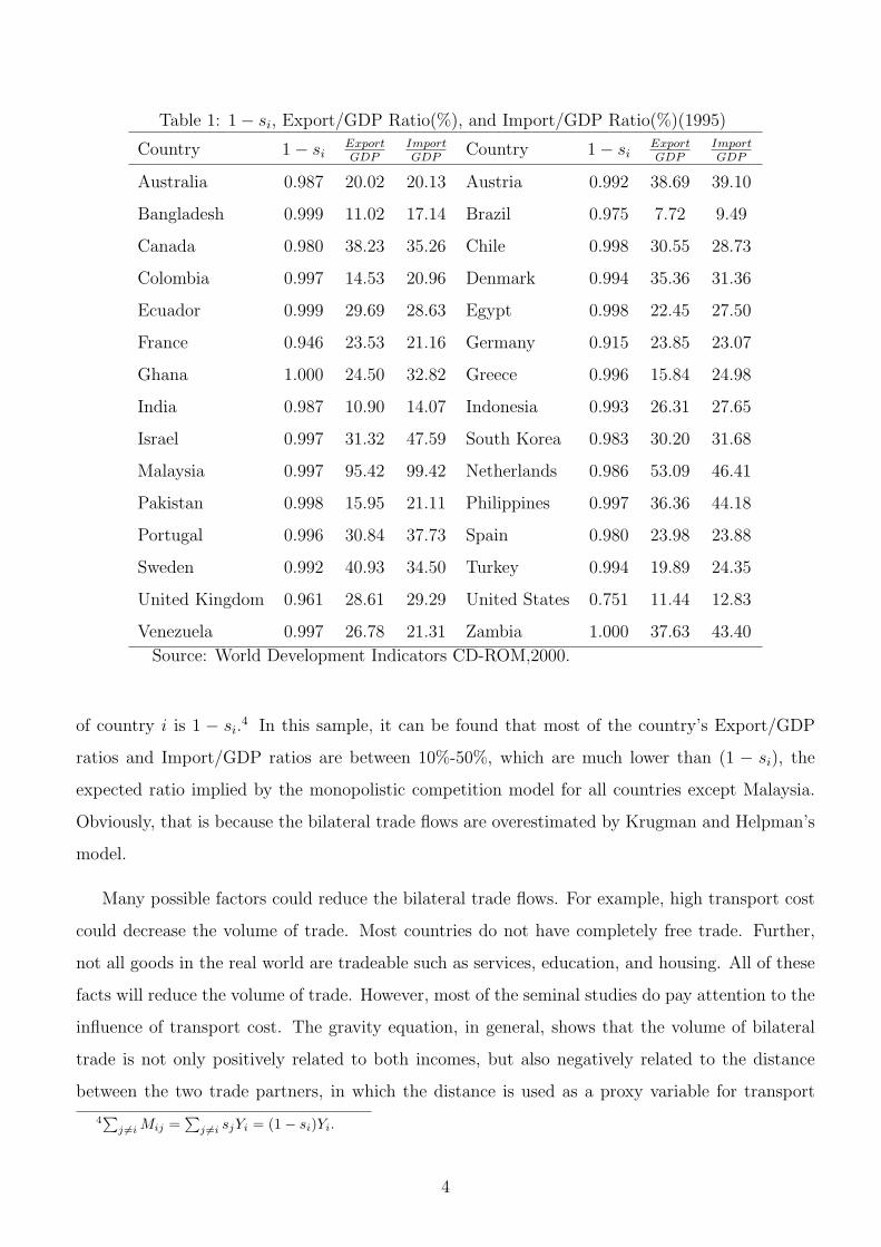
Table 1: 1− si, Export/GDP Ratio(%), and Import/GDP Ratio(%)(1995)

Country 1− siExportGDP

ImportGDP

Country 1− siExportGDP

ImportGDP

Australia 0.987 20.02 20.13 Austria 0.992 38.69 39.10

Bangladesh 0.999 11.02 17.14 Brazil 0.975 7.72 9.49

Canada 0.980 38.23 35.26 Chile 0.998 30.55 28.73

Colombia 0.997 14.53 20.96 Denmark 0.994 35.36 31.36

Ecuador 0.999 29.69 28.63 Egypt 0.998 22.45 27.50

France 0.946 23.53 21.16 Germany 0.915 23.85 23.07

Ghana 1.000 24.50 32.82 Greece 0.996 15.84 24.98

India 0.987 10.90 14.07 Indonesia 0.993 26.31 27.65

Israel 0.997 31.32 47.59 South Korea 0.983 30.20 31.68

Malaysia 0.997 95.42 99.42 Netherlands 0.986 53.09 46.41

Pakistan 0.998 15.95 21.11 Philippines 0.997 36.36 44.18

Portugal 0.996 30.84 37.73 Spain 0.980 23.98 23.88

Sweden 0.992 40.93 34.50 Turkey 0.994 19.89 24.35

United Kingdom 0.961 28.61 29.29 United States 0.751 11.44 12.83

Venezuela 0.997 26.78 21.31 Zambia 1.000 37.63 43.40

Source: World Development Indicators CD-ROM,2000.

of country i is 1 − si.4 In this sample, it can be found that most of the country’s Export/GDP

ratios and Import/GDP ratios are between 10%-50%, which are much lower than (1 − si), the

expected ratio implied by the monopolistic competition model for all countries except Malaysia.

Obviously, that is because the bilateral trade flows are overestimated by Krugman and Helpman’s

model.

Many possible factors could reduce the bilateral trade flows. For example, high transport cost

could decrease the volume of trade. Most countries do not have completely free trade. Further,

not all goods in the real world are tradeable such as services, education, and housing. All of these

facts will reduce the volume of trade. However, most of the seminal studies do pay attention to the

influence of transport cost. The gravity equation, in general, shows that the volume of bilateral

trade is not only positively related to both incomes, but also negatively related to the distance

between the two trade partners, in which the distance is used as a proxy variable for transport

4∑

j 6=i Mij =∑

j 6=i sjYi = (1− si)Yi.

4

costs.

The study of the gravity equation is probably the most successful empirical work in interna-

tional trade. The model was first introduced by Tinbergen (1962), in which the econometric model

of trade flows was based only on intuitive justification. Anderson (1979) was the first to derive

the gravity equation theoretically. Anderson (1979) assumed that preferences are Cobb-Douglas

(or CES) and the goods are differentiated by countries of origin, which is called the Armington

assumption. Bergstrand (1985) used CES preferences over Armington-differentiated goods to de-

velop a general equilibrium model of world trade , thus yielding a reduced-form gravity equation

for bilateral trade involving price indices.

The gravity equation model has been widely employed to infer substantial bilateral trade flow

effects. Aitken (1973) showed that European trade is significantly influenced by membership in

a trading community such as the European Economic Community (EEC) and the European Free

Trade Association (EFTA), and the neighboring country dummy variable. Geraci and Prewo

(1976) included average tariff rates, preferential trading group membership and common language

in a gravity model and found that these effects have a significant impact on bilateral trade flows

in a sample of OECD countries. Srivastava and Green (1986) incorporated some noneconomic

variables in a gravity model and found that cultural similarity, political instability, economic union

and former colonial status are all significant determinants of bilateral trade flows. Thursby and

Thursby (1987) found strong support for the hypothesis that increased exchange rate variability

affects bilateral trade flows. Recently, Bougheas, Demetriades and Morgenroth (1999) examined

the role of infrastructure in a bilateral trade model with transport costs and the empirical results

demonstrated that the level of infrastructure and the trade volume have a positive relationship.

Jensen (2000) modifies the gravity model by using disaggregated production data instead of

GDP as a measure of production for exporting countries. This is because nontraded goods are

included in GDP. Therefore, GDP is not considered as a good indicator of potential exports.

However, his gravity equation included a country’s income share, in which the nontraded goods

problem also exists. Helpman and Krugman (1985),5 discussed the model with the introduction

of nontraded goods. They characterize the integrated world equilibrium and the region of factor

price equalization when nontraded goods exist. However, they do not analyze the relationship

between the volume of trade and nontraded goods. Schmitt and Yu (2001) employ a monopolistic

competitive model with traded and non-traded goods to show that an increase in the degree of

economies of scale of production will increase the volume of intra-industry trade, which is the

5See Chapter 10.

5

finding of the empirical study of Harrigan (1994). To date, to the best of my knowledge, there

is no paper that includes nontraded goods in the gravity model and examines the relationship

between the consumption of nontraded goods and the volume of trade, even though nontraded

goods have an important impact upon bilateral trade flows.

In this paper, the assumption that all goods are tradable is relaxed. I incorporate nontraded

goods in a monopolistic competition model. This model tries to provide an explanation of why

the real volume of trade is much lower than predicted. The intuition is quite simple. It is because

the countries do not have so many goods that are tradable in the real world. An estimable gravity

equation can be derived from this model. Moreover, since this model incorporates nonhomothetic

preferences, it also can explain the phenomenon that the volumes of trade among the industrialized

countries are relative large to the volumes of trade between developed and less-developed countries,

which was proposed by Linder (1961) and Markusen (1986).6

The remainder of this paper is organized as follows: in Section 2, we set up the model and

derive the gravity equation with nontraded goods. The individuals consume differentiated tradable

goods as well as nontraded goods, and preferences are specificed as an additively separable utility

function. It shows that bilateral trade flow is not only related to the GDPs of importing and

exporting countries, but also is a function of the per capita income of both countries. The bilateral

trade flows are negatively related to the consumption of nontraded goods. Section 3 describes the

data sets used in this study. The empirical results are given in Section 4. They strongly support

the prediction of this model in a sample of 118 countries in 1995. Section 5 concludes.

The Model

In this section, the model is set up. Consider an open economy which has balanced trade, no

transport costs, and with identical production technologies. There are m countries and two types

of goods, tradeable goods (xk) and nontraded goods (z). The tradeable goods (xk) are differentiated

manufactured goods which are produced with production technologies with increasing returns to

scale. The nontraded good is a homogeneous commodity and is produced with a constant returns

to scale (CRS) technology.

6Markusen (1986) proposed a nonhomothetic model to explain the difference between the volume of W-E trade

and the volume of N-S trade. Unfortunately, his model does not offer a testable model to predict the volume of trade

from his model. However, in the extension of his paper, Hunter and Markusen (1988) proposed a nonhomothetic

model and estimated a linear expenditure system (LES) to show that the demand is nonhomothetic.

6

It is assumed that all individuals consume tradeable goods as well as nontraded goods. Con-

sumers have the following identical nonhomothetic preferences, which are given by

U = (Σkxαk )1/α + u(z), 0 < α < 1, (2)

where u(.) is a strictly concave function.

All individuals maximize their utility subject to their income. Since the subutility function for

differentiated goods is homogeneous of degree one, we can use a two-stage budgeting procedure to

solve this utility maximization problem.7 The consumer’s problem can be rewritten as

Max U = X + u(z), (3)

s.t. PX + pzz = I.

where I is individual income, X = (Σkxαk )1/α is the quantity index for differentiated goods, P =

(Σkpα/(α−1)k )(α−1)/α is the price index for X , and pz and pk for good z and xk, respectively.

If we consider X as the numeraire, the utility can be considered as a quasi-linear utility function.

According to the property of quasi-linear utility function, the consumption of z is constant which

is determined by

u′(z) =pz

P , (4)

for all consumers if the income is big enough. There is no income effect for z. Increasing individual

income does not change the quantity of demand for good z at all, and all the extra income goes

entirely to the consumption of differentiated goods. Let z = z∗ satisfy equation (4) which means

that z∗ is the demand quantity of notraded good for every consumer in every country and thus is

independent of individual income and the prices of the differentiated commodities. Furthermore,

it is also assumed that the individual’s income in every country is bigger than z∗. Due to this

special property of the nonhomothetic preference, the production of nontraded good for country i

is Zi = niz∗ and is produced first in country i, where ni is the population of country i.

In addition, the differentiated manufactured goods are produced and freely traded. Just like

the imperfect competition model proposed by Helpman and Krugman (1985) and Helpman (1987),

a number of firms produce one differentiated commodity in a monopolistically competitive market.

Also, all firms are equipped with identical IRS technology, and free entry leads to zero profit in

equilibrium.

7The detail of derivation is in the Appendix.

7

Table 2: An Example with Three Countries

Country Population Per Capita Income GDP Exporta

GDPExportb

GDP

A 10 10 100 0.6 0.3937

B 10 10 100 0.6 0.3937

C 10 5 50 0.8 0.35

a. the expected ratio of ExportGDP

in Helpman and Krugman’s model.

b. the expected ratio of ExportGDP

in this nontraded goods model.

In this model, the volume of trade is different from the result of Helpman and Krugman (1985)

and Helpman (1987) but similar. Since this property of nonhomothetic preference is “love for

variety” for differentiated goods, each country will demand all foreign varieties according to the

country’s share of world value of differentiated goods. Therefore, the value of differentiated goods

that country i imports from j, denoted Mij, is

Mij =XiXj

Xw

, (5)

where Xj is the value of a differentiated good produced in country j, and Xw = ΣjXj is the world

output of differentiated goods.

Let Yi = Xi +Zi denote the GDP of country i. Rearranging equation (5), Mij can be rewritten

as

Mij =(Yi − Zi)(Yj − Zj)

Σj(Yj − Zj)=

(Yi − niz∗)(Yj − njz

∗)Xw

. (6)

In the following, I take an example to show how this model can explain the question I proposed

in Section 1. Consider a three-country economy, consisting of countries A, B, and C. Suppose

that there are 10 people in each country and each individual consumes 3 units of nontraded goods.

Assume that the per capita income of A and B is 10 and the per capita income of C is 5. The

summary of this example is shown in Table 2. In the imperfect competition model, the expected

ratios of export over GDP for each country are 0.6, 0.6 and 0.8, respectively. However, the expected

ratios are reduced if we consider the influence of nontraded goods. As can be seen in Table 2, the

ratios are down to 0.3937, 0.3937 and 0.35, respectively. this can explain why the phenomenon in

Table 1 happened.

Another advantage of this model is that the expected Export/GDP ratio of a small country is

not necessary bigger than a large country. Since the Export/GDP ratio is 1− si in Helpman and

Krugman’s model, a country with a smaller GDP will have a larger Export/GDP ratio. However,

8

this is not consistent with the data. For example, since Colombia’s GDP is apparently smaller

than Germany’s GDP, the Export/GDP and/or Import/GDP ratios of Colombia are smaller than

Germany’s ratios in in Table 1, which is not consistent with Helpman and Krugman’s model.

However, it can be explained by Table 2.

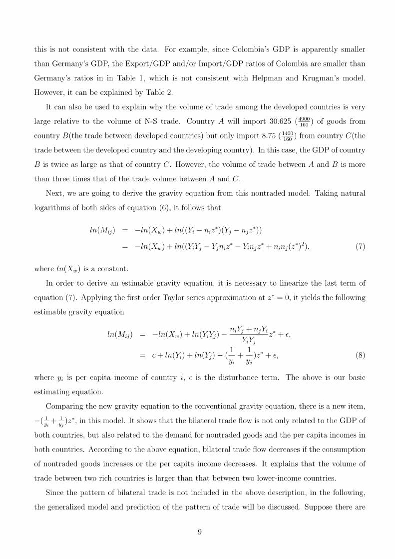
It can also be used to explain why the volume of trade among the developed countries is very

large relative to the volume of N-S trade. Country A will import 30.625 (4900160

) of goods from

country B(the trade between developed countries) but only import 8.75 (1400160

) from country C(the

trade between the developed country and the developing country). In this case, the GDP of country

B is twice as large as that of country C. However, the volume of trade between A and B is more

than three times that of the trade volume between A and C.

Next, we are going to derive the gravity equation from this nontraded model. Taking natural

logarithms of both sides of equation (6), it follows that

ln(Mij) = −ln(Xw) + ln((Yi − niz∗)(Yj − njz

∗))

= −ln(Xw) + ln((YiYj − Yjniz∗ − Yinjz

∗ + ninj(z∗)2), (7)

where ln(Xw) is a constant.

In order to derive an estimable gravity equation, it is necessary to linearize the last term of

equation (7). Applying the first order Taylor series approximation at z∗ = 0, it yields the following

estimable gravity equation

ln(Mij) = −ln(Xw) + ln(YiYj)− niYj + njYi

YiYj

z∗ + ε,

= c + ln(Yi) + ln(Yj)− (1

yi

+1

yj

)z∗ + ε, (8)

where yi is per capita income of country i, ε is the disturbance term. The above is our basic

estimating equation.

Comparing the new gravity equation to the conventional gravity equation, there is a new item,

−( 1yi

+ 1yj

)z∗, in this model. It shows that the bilateral trade flow is not only related to the GDP of

both countries, but also related to the demand for nontraded goods and the per capita incomes in

both countries. According to the above equation, bilateral trade flow decreases if the consumption

of nontraded goods increases or the per capita income decreases. It explains that the volume of

trade between two rich countries is larger than that between two lower-income countries.

Since the pattern of bilateral trade is not included in the above description, in the following,

the generalized model and prediction of the pattern of trade will be discussed. Suppose there are

9

three types of goods, X1, X2, and z. X1 and X2 are tradable and differentiated goods produced

by identical increasing return to scale technology. The definition of z is exactly as described.

Furthermore, it is assumed X1 is relatively capital-intensive compared with X2, and the modified

utility function is specified as

U = (Σxα1k + Σxα

2k)1/α + u(z), 0 < α < 1. (9)

Given the above assumptions and the result of Helpman and Krugman (1985), we can obtain

not only the result of equation (8), but also that a capital-abundant country imports labor-intensive

goods from a labor-abundant country.

Data

There are three databases used in this study. The world bilateral trade flows data is originally

obtained from the CD-ROM “World Trade Flows, 1980-1997, with Production and Tariff Data,”

which is available from the Social Science Data Service, Institute of Governmental Affairs, Uni-

versity of California, Davis. The data used to test this model is from the year of 1995. There are

182 countries or regions in this database. In Feenstra (2000), it indicated that the main source for

bilateral trade data is the United National Statistical Office. Those data were also published in

the Yearbook of International Trade Statistics and fully reported in Commodity Trade Statistics

by the United Nation.

Another data set used in the study is the GDP and per capita income data which is downloaded

from Harvard University, CID(Center for International Development). The GDP and per capita

income are PPP-adjusted. In Gallup and Sachs (1999), it indicated that most of the GDP and per

capita income data are from the World Bank (1997, 1998). For countries which are missing in the

World Bank, the data is obtained from CIA (1996,1997).

In order to compare this nontraded goods model and the conventional gravity model, a distance

data set is also employed. The distance data set is downloaded from Purdue University.8 This

data set contains 137 countries and it provides the distance between capital cities in kilometers.

Combining the above three data sets, there are 118 countries employed in this paper. The

names of those countries are listed in the Appendix. From the Appendix, it can be found that

almost all of the countries or regions in the world are included.

8ftp://intrepid.mgmt.purdue.edu/pub/Trade.Data/dist.txt.

10

Empirical Results

In this section, the gravity equations derived from the nonhomothetic model are estimated by using

the above data set. Based on equation (8), the gravity equation can be specified as the following

two forms

ln(Mij) = α + β1ln(Yi) + β2ln(Yj)− z∗(1

yi

+1

yj

) + ε, (10)

or

ln(Mij) = α + βln(YiYj)− z∗(1

yi

+1

yj

) + ε, (11)

where α, β and z∗ are the coefficients to be estimated. Theoretically, α is expected to be negative,

z∗ should be positive, and β1 and β2 should be around 1.

In order to demonstrate the advantage of this new model, the conventional gravity equation is

also to be estimated, which is

ln(Mij) = α + β1ln(Yi) + β2ln(Yj) + ε. (12)

Ordinary Least Square(OLS) estimation is employed to estimate the above regressions. The

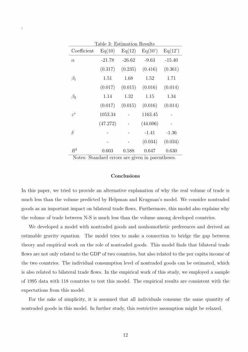
estimation results are shown in Table 3. There are 13,806 observations in this sample. In Table 3,

it shows all of the estimated coefficients in equation (10) and (12) are significant at 1% significant

level. The most important is that all of the signs of the estimated coefficients coincide with our

expectation. In particular, z∗ is around $1,053 in this model, which means that all individuals

consume at least about $1,053 goods produced by their country every year. Comparing to Eq(12),

it can be found that the estimated coefficients of GDPs in Eq(10) are significant closer to unity than

in Eq(12) which means that this new model has a theoretical advantage. This nontraded goods

gravity equation is more consistent with the data than the conventional gravity model. The R2 of

Eq(10) is about 0.60, which is bigger than the R2 in Eq(12). That shows that the goodness-of-fit

of this new model is better than the conventional model.

Next, I examine the performance of this model when a distance term exists and compare

the traditional gravity equation with a distance term. The results are also given in Table 3 where

Eq(10’) and Eq(12’) are Eq(10) and Eq(12) with distance term, respectively. The δ is the coefficient

of the distance term in each model. Just like the results above, the signs of estimated coefficients

are as expected and significant. We also can find that the estimated coefficients of GDPs are also

much closer to unity than the result of Eq(12’).

11

,

Table 3: Estimation Results

Coefficient Eq(10) Eq(12) Eq(10’) Eq(12’)

α -21.78 -26.62 -9.63 -15.40

(0.317) (0.235) (0.416) (0.361)

β1 1.51 1.68 1.52 1.71

(0.017) (0.015) (0.016) (0.014)

β2 1.14 1.32 1.15 1.34

(0.017) (0.015) (0.016) (0.014)

z∗ 1053.34 - 1163.45 -

(47.272) - (44.606) -

δ - - -1.41 -1.36

- - (0.034) (0.034)

R2 0.603 0.588 0.647 0.630

Notes: Standard errors are given in parentheses.

Conclusions

In this paper, we tried to provide an alternative explanation of why the real volume of trade is

much less than the volume predicted by Helpman and Krugman’s model. We consider nontraded

goods as an important impact on bilateral trade flows. Furthermore, this model also explains why

the volume of trade between N-S is much less than the volume among developed countries.

We developed a model with nontraded goods and nonhomothetic preferences and derived an

estimable gravity equation. The model tries to make a connection to bridge the gap between

theory and empirical work on the role of nontraded goods. This model finds that bilateral trade

flows are not only related to the GDP of two countries, but also related to the per capita income of

the two countries. The individual consumption level of nontraded goods can be estimated, which

is also related to bilateral trade flows. In the empirical work of this study, we employed a sample

of 1995 data with 118 countries to test this model. The empirical results are consistent with the

expectations from this model.

For the sake of simplicity, it is assumed that all individuals consume the same quantity of

nontraded goods in this model. In further study, this restrictive assumption might be relaxed.

12

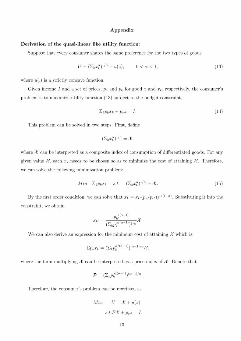
Appendix

Derivation of the quasi-linear like utility function:

Suppose that every consumer shares the same preference for the two types of goods:

U = (Σkxαk )1/α + u(z), 0 < α < 1, (13)

where u(.) is a strictly concave function.

Given income I and a set of prices, pz and pk for good z and xk, respectively, the consumer’s

problem is to maximize utility function (13) subject to the budget constraint,

Σkpkxk + pzz = I. (14)

This problem can be solved in two steps. First, define

(Σkxαk )1/α = X .

where X can be interpreted as a composite index of consumption of differentiated goods. For any

given value X , each xk needs to be chosen so as to minimize the cost of attaining X . Therefore,

we can solve the following minimization problem:

Min Σkpkxk s.t. (Σkxαk )1/α = X . (15)

By the first order condition, we can solve that xk = xk′(pk/pk′))1/(1−α). Substituting it into the

constraint, we obtain

xk′ =p

1/(α−1)k′

(Σkpα/(α−1)k )1/α

X .

We can also derive an expression for the minimum cost of attaining X which is:

Σpkxk = (Σkpα/(α−1)k )(α−1)/αX .

where the term multiplying X can be interpreted as a price index of X . Denote that

P = (Σkpα/(α−1)k )(α−1)/α.

Therefore, the consumer’s problem can be rewritten as

Max U = X + u(z),

s.t.PX + pzz = I.

13

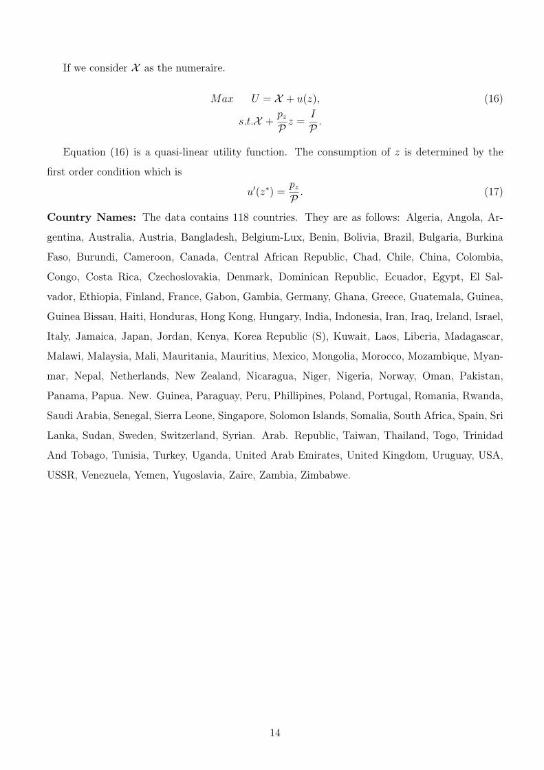
If we consider X as the numeraire.

Max U = X + u(z), (16)

s.t.X +pz

P z =I

P .

Equation (16) is a quasi-linear utility function. The consumption of z is determined by the

first order condition which is

u′(z∗) =pz

P . (17)

Country Names: The data contains 118 countries. They are as follows: Algeria, Angola, Ar-

gentina, Australia, Austria, Bangladesh, Belgium-Lux, Benin, Bolivia, Brazil, Bulgaria, Burkina

Faso, Burundi, Cameroon, Canada, Central African Republic, Chad, Chile, China, Colombia,

Congo, Costa Rica, Czechoslovakia, Denmark, Dominican Republic, Ecuador, Egypt, El Sal-

vador, Ethiopia, Finland, France, Gabon, Gambia, Germany, Ghana, Greece, Guatemala, Guinea,

Guinea Bissau, Haiti, Honduras, Hong Kong, Hungary, India, Indonesia, Iran, Iraq, Ireland, Israel,

Italy, Jamaica, Japan, Jordan, Kenya, Korea Republic (S), Kuwait, Laos, Liberia, Madagascar,

Malawi, Malaysia, Mali, Mauritania, Mauritius, Mexico, Mongolia, Morocco, Mozambique, Myan-

mar, Nepal, Netherlands, New Zealand, Nicaragua, Niger, Nigeria, Norway, Oman, Pakistan,

Panama, Papua. New. Guinea, Paraguay, Peru, Phillipines, Poland, Portugal, Romania, Rwanda,

Saudi Arabia, Senegal, Sierra Leone, Singapore, Solomon Islands, Somalia, South Africa, Spain, Sri

Lanka, Sudan, Sweden, Switzerland, Syrian. Arab. Republic, Taiwan, Thailand, Togo, Trinidad

And Tobago, Tunisia, Turkey, Uganda, United Arab Emirates, United Kingdom, Uruguay, USA,

USSR, Venezuela, Yemen, Yugoslavia, Zaire, Zambia, Zimbabwe.

14

References

Aitken, Norman D. (1973), “The Effect of the EEC and EFTA on European Trade: A Temporal

Cross-Section Analysis,” American Economic Review, 63, 881-892.

Anderson, James E. (1979), “A Theoretical Foundation for the Gravity Equation,” American

Economic Review, 69, 106-116.

Bergstrand, Jeffrey (1985), “The Gravity Equation in International Trade: Some Microeconomic

Foundations and Empirical Evidence,” Review of Economics and Statistics, 67, 474-481.

Bougheas, Spiros, Demetriades, Panico O. and Edgar L.W. Morgenroth (1999), “Infrastructure,

Transport Cost and Trade,” Journal of International Economic, 47, 169-189.

CIA (1996) The World Factbook. Washington, D.C. Central Intelligence Agency.

CIA (1997) The World Factbook. http://www.odci.gov/cia/publications/factbook/index.html.

Feenstra, Robert C. (2000), “World Trade Flows, 1980-1997, with Production and Tariff Data,”

Working Paper, University of California, Davis.

Gallup, John L. and Jeffery D. Sachs (1999), “Geography and Economic Development,” Working

Paper, Harvard University.

Geraci, Vincent J. and Wilfried Prewo (1977), “Bilateral Trade Flows and Transport Costs,”

Review of Economics and Statistics, 59, 67-74.

Harrigan, James (1994), “Scale Economies and the Volume of Trade,” Review of Economics and

Statistics, 76, 321-328.

Helpman, Elhanan (1987),“Imperfect Competition and International Trade: Evdience from Four-

teen Industrial Countries,” Journal of the Japanese and International Economies, 1, 62-81.

Helpman, Elhanan and Paul Krugman (1985), Increasing Returns, Imperfect Competition, and

Foreign Trade, Cambridge: MIT Press.

Hunter, Linda and James R. Markusen (1988), “Per Capita Income as a Basis for Trade,” in:

Robert Feenstra, ed., Empirical Methods for International Trade, Cambridge: MIT Press.

Hunter, Linda (1991), “The Contribution of Nonhomothetic Preferences to Trade,” Journal of

International Economics, 30, 345-358.

15

Jensen, Paul E. (2000), “ Analysis of Bilateral Trade Patterns with Panel Data,” Review of

International Economics, 8, 86-99.

Linder, Staffan B. (1961), An Essay on Trade and Transformation, New York: Wiley and Sons.

Markusen, James R. (1986), “Explaining the Volume of Trade: An Eclectic Approach,” American

Economic Review, 76, 1002-1011.

Schmitt, Nicolas and Zhihao Yu (2001), “Economies of Scale and the Volume of Intra-Industry

Trade,” Manuscript.

Srivastava, Rajendra K. and Robert T. Green (1986), “Determinants of Bilateral Trade Flows,”

Journal of Business, 59, 623-640.

Thursby, Jerry G. and Marie C. Thursby (1987), “Bilateral Trade Flows, the Linder Hypothesis,

and Exchange Risk,” Review of Economics and Statistics, 69, 488-495.

Tinbergen, Jan (1962), Shaping the World Economy: Suggestions for an International Economic

Policy, New York: Twentieth Century Fund.

World Bank. (1997) World Development Indicators 1997 CD-ROM. Washington, D.C.: Interna-

tional Bank for Reconstruction and Development.

World Bank. (1998) World Development Indicators 1998 CD-ROM. Washington, D.C.: Interna-

tional Bank for Reconstruction and Development.

16

CHAPTER III

ARBITRAGE AND THE HARMONIZATION OF PATENT LIVES

Introduction

The primary purpose of intellectual property rights (hereinafter IPRs) protection is to provide

innovators incentives to develop new technologies, products, and services. IPRs grant innovators

monopoly power to make profits on their innovations, which also generates additional consumer

surplus. The cost of providing IPRs protection is that it permits innovators to exercise monopoly

power over the market, which prevents the benefits of the new products from being enjoyed opti-

mally by consumers. There exists a trade-off between static deadweight loss and dynamic gains

from innovation. Therefore, in a closed economy, the existing literature(e.g. Nordhaus (1969),

Scherer (1980), and Deardorff (1992)) suggests that IPRs should be granted only for a limited

period.

Recently, IPRs protection has gained importance in international trade. Maskus (2000) in-

dicates that IPRs protection has been at the forefront of global economic policymaking, and a

number of countries have strengthened their laws and regulations regarding IPRs protection. Es-

pecially, the agreement on Trade-Related Aspects of Intellectual Property Rights (TRIPs) was

concluded as a part of the foundation of the World Trade Organization (WTO).

Studying IPRs protection in an open economy introduces additional complications, since there

are two types of externality involved. One is the terms of trade externality because, for example,

it worsens the home country terms of trade on patented products if IPRs protection is granted

in the foreign country. The foreign consumer surplus would be diminished by the exercise of

monopoly power. The other is the property of public goods since the foreign country benefits

from the creation of consumer surplus by the introduction of new innovations in the home country.

Thus, an increase in domestic patent length will encourage domestic innovators as well as foreign

innovators, but it only negatively affects the domestic consumers’ surplus. Therefore, each country

hopes that its trading partners can strengthen their level of protection and it can lower its own

level of protection, which creates a prisoner’s-dilemma-like situation.

Lai and Qiu (2003) utilize a game-theoretical approach to analyze international IPRs protection

in a multi-sectoral two-country model . They show that, in Nash equilibrium, developed countries

17

(North) have a stronger incentive to protect IPRs than developing countries (South), which explains

why the North chooses a longer IPRs standard than the South. They also find that global welfare

increases if developing countries increase their IPRs standards. Grossman and Lai (2004) propose

an infinite horizon general equilibrium model in which each firm innovates in every period. They

examine the IPRs policy in two countries that differ in market size, capacity, and wage rate.

Furthermore, their model demonstrates that harmonization in patent length is not necessary for

efficiency. Readjustments of patent protection across countries that leave global profits unaffected

will not affect world welfare. In their model, the issue of whether or not to harmonize primarily

affects the distribution of the income between the countries.

The existing literature suggests that the South has an incentive to provide IPRs protection

whether or not southern firms have capacities to innovate. However, the protection in the South is

weaker than in the North. The length of patent protection in developed countries is longer than in

developing countries because they have bigger markets and greater capacities for innovation. An

important feature of these models is the assumption that markets can be perfectly segmented, so

that IPRs protection of different lengths can be maintained without the interference of arbitrage

between markets.

In this paper, the assumption of perfect segmentation is relaxed. The existence of arbitrage

between international markets is hardly new, as evidenced by the importation of Canadian drugs.

The Minnesota Senior Federation, according to Weil (2004), organized its first prescription-drug-

buying bus trip to Canada in 1995. The bus picked up seniors in Minneapolis and drove them to

Winnipeg Canada, where they could purchase their prescription drugs at reduced prices. The bus

still runs eight or nine times a year. Currently, the Federation also runs two Internet pharmacy

stores, from which more than 4,000 customers ordered more than two million dollars worth of

drugs last year. Weil explains that the Federation’s activity has spurned the implementation of

similar bus trips in California, Arizona, Maine and other border states.

Some Canadian pharmacies have also been soliciting business in the US, where drug prices are

substantially higher. The internet, which is easily accessible, has encouraged this kind of arbitrage

behavior. The Wall Street Journal (Spors, 2004) reports that Americans bought approximately

$1.1 billion of Canadian drugs last year. Furthermore, some state governments also encourage this

kind of arbitrage. For example, Minnesota, New Hampshire, North Dakota and Wisconsin have all

constructed Web sites that instruct their residents how to buy relatively cheap prescription drugs

from Canadian pharmacies online. (State Legislatures, 2004).

Another example is the trade in illegal compact-discs, videotapes and video games in China

18

prior to the TRIPs agreement. The Economist (1996) reports that China produced 54 million

units of CDs in 1994, of which 88 percent of them were pirated. The Chinese bought under 40

million units themselves and the excess was exported. The United States bought 13% of pirated

sales by value. Americans bought more pirated music than any other country except Russia.

In the following, we examine how the existence of arbitrage affects the incentives for countries

in the setting of patent protections. We first examine the Nash equilibrium of the patent game

between countries when the patent agreement does not exist. We then show that the innovating

countries are not willing to completely eliminate arbitrage when the patent expires first in non-

innovating countries but is still effective in innovating countries, even when enforcement is costless.

We also show that the existence of arbitrage makes it more attractive for non-innovating countries

to strengthen their IPRs protection. Finally, we investigate the efficient international patent

agreement between countries. We show that the existence of arbitrage will result in efficient

patent agreements in which differences in patent levels across countries reduce the deadweight loss

within the patent system.

The remainder of this paper is organized as follows: In Section 2, we develop a two-country

model of intellectual property rights protection in which the markets are not completely segmented.

In Section 3, we show how arbitrage affects international IPRs protection and that there exists a

pure-strategy Nash equilibrium when arbitrage occurs after the patent protection first expires in

the non-innovating country. The efficient international patent agreement is examined in Section

4. Section 5 gives conclusions.

The Model

In this section, we set up a two-country model of IPRs protection in which the markets are not

completely segmented. Consider an economy with two countries, named South (s) and North (n),

and a variety of firms that develop new products in the North.1 The model follows Deardorff (1992)

and Scotchmer (2004) by considering a two-period model of innovation. It is assumed that there

are two sectors, a homogenous good sector and a differentiated products sector. In the first period,

firms choose the number of differentiated products to be produced and sold in the two markets in

1This assumption is not so restrictive. Braga (1990) indicates that developing countries only hold 1% of existing

patents. Chin and Grossman (1990), Diwan, and Rodrick (1991) and Deardorff (1992) make the same assumption

in their model. Furthermore, the main results in Grossman and Lai (2004) will not change if their assumption is

simplified.

19

the second period. Individuals are assumed to have identical preferences in each country. Each

consumer chooses zt and xt(ω) to maximize his utility which is given by:

∫ T

0

[

∫ N

0

u(xt(ω))dω + zt]e−ρtdt,

subject to

∫ N

0

pt(ω)xt(ω)dω + zt = Yt, for all t,

where T is the length of the production period, ω is the index of differentiated goods, N is the

measure of new differentiated products in the North, 0 < ρ < 1 is a discount factor, xt(ω) is the

consumption of a differentiated good ω at time t, zt is the consumption of the homogenous good,

and Yt is the current income. We assume that u′ > 0 and u′′ < 0. The first order condition yields

xt(ω) = x(pt(ω)) where x = (u′)−1.2 The demand for the numeraire good is given by:

zt = Yt − pt(ω)xt(pt(ω)).

The indirect utility function can be written as:

U =

∫ T

0

∫ N

0

s(pt(ω))dωe−ρtdt + Y,

where s(pt(ω)) = u(xt(pt(ω)))−pt(ω)xt(pt(ω)) is the consumer surplus associated with a represen-

tative differentiated product, Y is the present value of income during the production period. The

two-period model can be thought of as representing the steady state of an infinite horizon general

equilibrium model in which firms innovate in every period and products have an exogenously given

useful life, as has been shown by Grossman and Lai (2004).

Suppose that manufacturing requires only labor. Since the homogenous good z is considered as

the numeraire, without loss of generality, we assume that the production of the homogeneous good

z requires one unit of labor per unit of output and the market for z is competitive, which makes

the price of z equal to one. Furthermore, suppose that the production of one unit of all varieties of

differentiated products requires c units of labor. Under perfect segmentation, the innovating firms

are granted monopoly power over its goods when the patent is still in effect.

In this model, it is assumed that markets are imperfectly segmented, so an arbitrageur has

incentives to make a profit by exporting differentiated products from the low-price market to

2A utility function of this kind greatly simplifies the analysis. Krugman (1992) argues in favor of using this

kind of utility function for analyzing political economy issues in a multisectoral general equilibrium framework.

He indicates that, in such a framework, partial equilibrium intuition continues to apply in a general equilibrium

model. Currently, this is the standard model employed in the political economy literature on trade policy, such as

Grossman and Helpman (1994), Mitra (1999), Grossman and Lai (2004).

20

the high-price market. Potential arbitrage profits arise from two possibilities. The first is that

the manufacturers are price discriminating across markets when patents are still in effect in both

markets. This occurs when one manufacturer owns patents or national trademarks in several

markets. The producer would rationally set low prices in low-income countries, or in the markets

with elastic demand. In contrast, high-income countries, or inelastic-demand markets will face

a higher price. The purpose of differential pricing is in order to make a higher profit for the

manufacturer. However, since price differences exist between countries, there are incentives for

one to purchase goods in a low-price country and resell them in a high-price country if transaction

costs are low.

The second possibility occurs when the length of patent protection differs across markets. After

the patent expires in one market, imitators can freely produce the products at a constant cost c.

The market becomes competitive and the price drops to its marginal production cost, c, so that

the manufacturer can not make any profit. Since we focus on the impact of different patent lives

across markets, we assume that the demand for each innovation is the same for consumers in the

two markets, in the interest of simplicity. The only difference between the two markets is the

market size, xs(p) = Mxn(p) and ss(p) = Msn(p), where M denotes the relative market size of

the southern market.3 Furthermore, the profit function is assumed to be strictly concave on [c, p],

where π(c) = π(p) = 0.

Let λ denote the probability that goods which are legally protected from arbitrage are con-

fiscated by the government. This represents the level of enforcement against illegal arbitrage.

Therefore, the arbitrageur’s expected revenue is p(1−λ) for shipping a unit of differentiated prod-

uct from the South where its unit cost is c. Since arbitrage is subject to free entry, the zero profit

condition will force the market price equal to c/(1 − λ). Therefore, the patent holder will set its

price a little lower than c/(1− λ) to get the whole market. Thus, if λ = 0, the market price p will

be equal to c. We also can get p = pm, the monopoly price, for λ ≥ λ with pm = c/(1 − λ). The

market price falls and the volume of consumption increases when λ shrinks. On the other hand,

consumers’ surplus will increase. Furthermore, it is easy to show that, for λ ∈ [0, λ], there exists

a one-to-one relationship between λ and the market price, p(λ), with p′(λ) > 0.

In order to construct the payoff function for the Northern innovators, we assume that the patent

expires first in the South, i.e., tn ≥ ts where ti is the length of patent protection in country i.4

The conditions under which this will hold in the Nash equilibrium will be discussed below. Thus,

3This assumption follows Grossman and Lai (2004).4We will discuss the case of tn < ts in the Appendix.

21

we can get that pnt (ω) = ps

t(ω) = pm for t ≤ ts and pnt (ω) = ps

t(ω) = c for t > tn. For t ∈ (ts, tn],

pst(ω) = c and pn

t (ω) = p(λ) =min {c/(1 − λ), pm}. The average profits of an innovation during

the production period can be written as:

Π(τs, τn, λ, N) = (1 + M)τsπ(pm) + (τn − τs)π(p(λ)), (1)

where τn = 1−e−ρtn

1−e−ρT and τs = 1−e−ρts

1−e−ρT are the shares of the production period in which the product

is under IPRs protection in the North and South, respectively. The expression π(pm) is the

(monopoly) profit of a new product per period in the North, while π(p(λ)) is the firm profit when

the Northern government chooses λ as the enforcement level to prevent arbitrage after the patent

expires in the South.

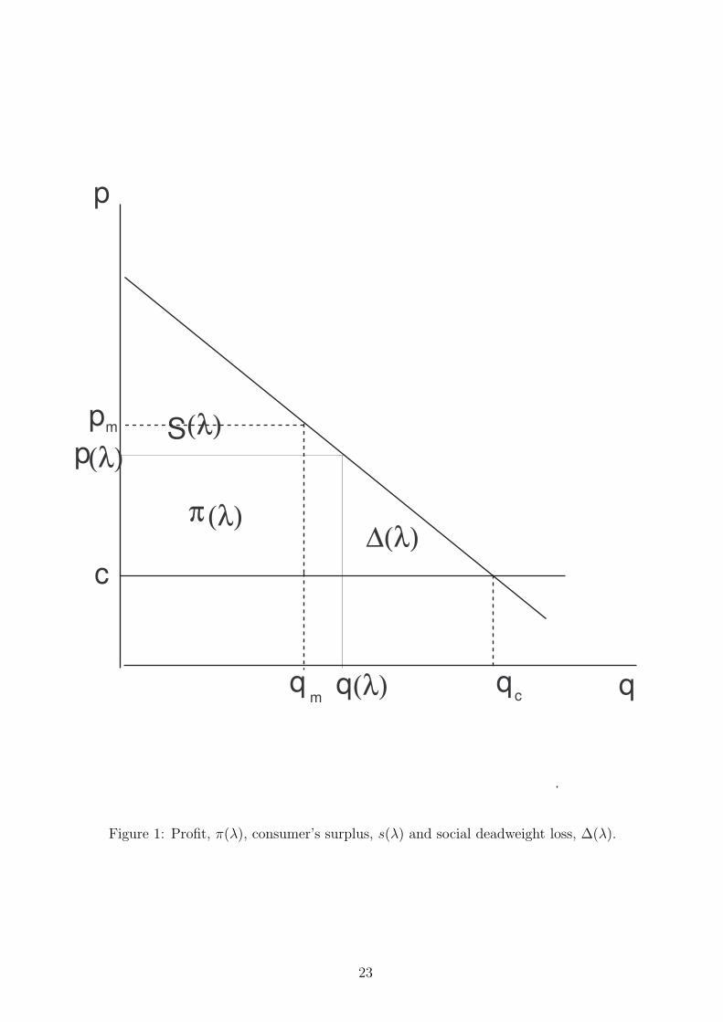
The demand function and the profit for a particular enforcement level for a representative

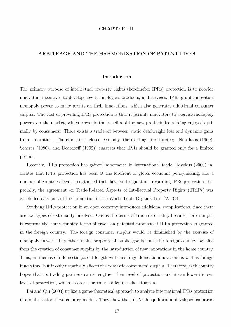
innovation are illustrated in Figure 1. In Figure 1, ∆(λ) is the social deadweight loss and s(λ)

is the consumer’s surplus. Since p′(.) is positive, we can see that a decrease in λ will increase

the consumer’s surplus and reduce social deadweight loss. The benefit of an innovation is the

monopolistic profits in the two countries during the life of the patent plus the profit in the North

after the patent expires in the South.

According to the definition of τi, there exists a one-to-one relationship between ti and τi. For

the sake of simplicity, we designate τi as the length of patent protection in the following model.

The goal of the government is to maximize the welfare of its country by choosing its policy tools,

the length of the patent(τi) and λ. The welfare of country i is the sum of firms’ profits in the two

countries and consumers’ surplus minus the cost of innovation and enforcement. Therefore, the

Northern government’s objective function is:

Wn(τs, τn, λ, N) = (τs(1 + M)π(pm) + (τn − τs)π(p(λ)))N (2)

+(τss(pm) + (1− τn)s(c) + (τn − τs)s(p(λ)))N − C(N)−G(λ).

The first part of the right hand side (hereinafter RHS) of equation (2) is the manufacturer’s

profit in both markets during the time when the patent has not expired. The profit from the

Southern market is τsMπ(pm). While the Southern patent has not expired, firms can make a

monopoly profit π in the North. When the Southern patent expires, but the Northern patent

remains in effect, firms can only make π(p(λ)). Therefore, producers can make [τsπ(pm) + (τn −τs)π(p(λ))] from the Northern market.

The second part of the North’s welfare is the consumers’ surplus. The Northern consumers’

surplus is s(pm) before the Southern patent expires, s(c) after the Northern patent expires, and

22

c

π

S

q

p

qqcm

q

(λ)

(λ)

(λ)

(λ)p

∆(λ)

pm

Figure 1: Profit, π(λ), consumer’s surplus, s(λ) and social deadweight loss, ∆(λ).

23

s(p(λ)) when the patent expires in the South but remains in effect in the North, with an enforcement

level, λ.

The third part of RHS of equation (2) is the innovation cost. C(N) denotes the cost of

innovation required to generate N innovations in the North. Suppose that C(.) is strictly convex

in N . This model follows Grossman and Lai (2004), and considers that increasing marginal costs

of producing innovations can arise from the existence of a sector-specific human capital input

employed in the R&D sector along with mobile labor.

The final part, G(λ), is the government cost of resources devoted to preventing arbitrage. G′(.)

is supposed to be positive which implies that the enforcement cost is increasing in enforcement

level, λ.

Similarly, we also can obtain the welfare for the South:

Ws(τs, N) = M(τss(pm) + (1− τs)s(c))N. (3)

Equation (3) indicates that the welfare of the non-innovating country only comes from its

consumers’ surplus, as the South’s buyers consume the differentiated goods invented in the North.

The Non-Cooperative Equilibrium

In this section, we analyze the Nash equilibrium of this patent-length setting game. We assume

that the sequence of decision is as follows: First, based on the welfare functions, governments

simultaneously set their patent length, τi, and the level of enforcement, λ.5 Then, the innovators

in the North decide how many innovations they plan to invent and sell their products in the two

markets. Since we are interested in the interaction between the two governments, the equilibrium

concept employed here is Nash equilibrium.

In stage 2, whether or not a firm decides to develop an innovation is determined by the marginal

profit and the marginal cost. Firms will invest in R&D up to the point where the cost of introducing

an additional innovation is equal to the benefit from the innovation, C ′(N∗) = Π. Therefore, the

optimal number of innovations can be expressed as a function of the enforcement level and the two

patent lengths, N∗ = N∗(τs, τn, λ).

5It is not reasonable if the North chooses λ first and then two countries choose τn and τs. If the two countries

choose τn and τs first, it does not affect the main conclusion of this paper in Proposition 1, in which the innovating

country does not have an incentive to completely eliminate arbitrage after the patent expires in the non-innovating

country.

24

Totally differentiating C ′(N∗(τs, τn, λ)) = Π(τs, τn, λ, N∗(τs, τn, λ)) yields:

dN∗

N∗ =[(π(1 + M)− π(p))dτs + π(p)dτn + (τn − τs)π

′(p)p′(.)dλ]γ

Π, (4)

where γ = C ′(N∗)/(N∗C ′′(N∗)) is the elasticity of innovation with respect to an increase in the

profit from innovation. An increase in patent length in either market will increase the profits from

innovation. Thus, it provides innovators incentives to increase the amount of innovation. Further-

more, strengthening the enforcement level also will increase the number of inventions because the

profits returned from an innovation improve.

Substituting N∗(τs, τn, λ) into equation (2), the North’s welfare function can be rewritten as

Wn(τs, τn, λ) = Wn(τs, τn, λ, N∗(τs, τn, λ)). (5)

Similarly, the South’s welfare function can be rewritten as

Ws(τs, τn, λ) = Ws(τs, N∗(τs, τn, λ)). (6)

In stage 1, the North’s government chooses the enforcement level and patent length. Taking the

derivative of equation (5) with respect to λ, τn, we can obtain the following first order conditions:

∂Wn

∂λ=

∂Wn

∂λ+

∂Wn

∂N∗∂N∗

∂λ

= (τn − τs)(π′(p(λ)) + s′(p(λ)))p′(λ)N∗ (7)

+ (τss(pm) + (1− τn)s(c) + (τn − τs)s(p(λ)))(τn − τs)π

′(p(λ))p′(λ)N∗γΠ

−G′(λ) = 0,

and

∂Wn

∂τn

=∂Wn

∂τn

+∂Wn

∂N∗∂N∗

∂τn

= (π(p(λ)) + s(p(λ))− s(c))N∗ (8)

+ (τss(pm) + (1− τn)s(c) + (τn − τs)s(p(λ)))π(p(λ))N∗γΠ

= 0.

In the South, the government has one decision to make. The necessary condition is:

∂Ws

∂τs

=∂Ws

∂τs

+∂Ws

∂N∗∂N∗

∂τs

= (s(pm)− s(c))MN∗

+ M(τss(pm) + (1− τs)s(c))(π(1 + M)− π(p(λ)))N∗γ

Π= 0. (9)

In order simplify our analysis, we assume that enforcement against illegal arbitrage is costless

(i.e. G(.) = 0), in section 3 and section 4.6 The pure Nash equilibrium can be solved by equations

(7), (8) and (9). Next, we characterize the properties of the Nash equilibrium.

6It is surprising that we will find that the North will not choose to completely eliminate arbitrage even though

enforcement is costless.

25

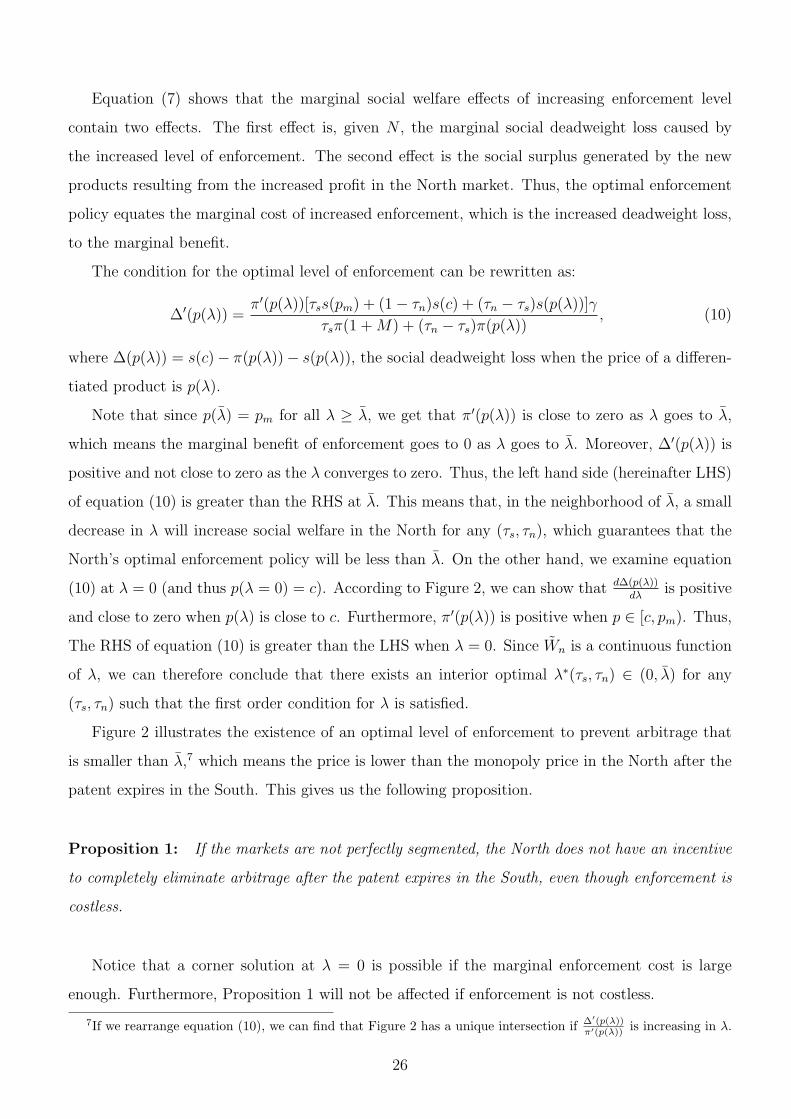
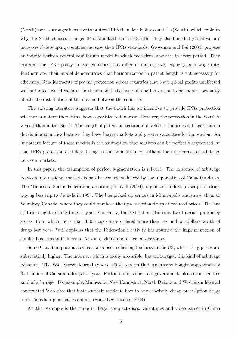
Equation (7) shows that the marginal social welfare effects of increasing enforcement level

contain two effects. The first effect is, given N , the marginal social deadweight loss caused by

the increased level of enforcement. The second effect is the social surplus generated by the new

products resulting from the increased profit in the North market. Thus, the optimal enforcement

policy equates the marginal cost of increased enforcement, which is the increased deadweight loss,

to the marginal benefit.

The condition for the optimal level of enforcement can be rewritten as:

∆′(p(λ)) =π′(p(λ))[τss(pm) + (1− τn)s(c) + (τn − τs)s(p(λ))]γ

τsπ(1 + M) + (τn − τs)π(p(λ)), (10)

where ∆(p(λ)) = s(c)− π(p(λ))− s(p(λ)), the social deadweight loss when the price of a differen-

tiated product is p(λ).

Note that since p(λ) = pm for all λ ≥ λ, we get that π′(p(λ)) is close to zero as λ goes to λ,

which means the marginal benefit of enforcement goes to 0 as λ goes to λ. Moreover, ∆′(p(λ)) is

positive and not close to zero as the λ converges to zero. Thus, the left hand side (hereinafter LHS)

of equation (10) is greater than the RHS at λ. This means that, in the neighborhood of λ, a small

decrease in λ will increase social welfare in the North for any (τs, τn), which guarantees that the

North’s optimal enforcement policy will be less than λ. On the other hand, we examine equation

(10) at λ = 0 (and thus p(λ = 0) = c). According to Figure 2, we can show that d∆(p(λ))dλ

is positive

and close to zero when p(λ) is close to c. Furthermore, π′(p(λ)) is positive when p ∈ [c, pm). Thus,

The RHS of equation (10) is greater than the LHS when λ = 0. Since Wn is a continuous function

of λ, we can therefore conclude that there exists an interior optimal λ∗(τs, τn) ∈ (0, λ) for any

(τs, τn) such that the first order condition for λ is satisfied.

Figure 2 illustrates the existence of an optimal level of enforcement to prevent arbitrage that

is smaller than λ,7 which means the price is lower than the monopoly price in the North after the

patent expires in the South. This gives us the following proposition.

Proposition 1: If the markets are not perfectly segmented, the North does not have an incentive

to completely eliminate arbitrage after the patent expires in the South, even though enforcement is

costless.

Notice that a corner solution at λ = 0 is possible if the marginal enforcement cost is large

enough. Furthermore, Proposition 1 will not be affected if enforcement is not costless.

7If we rearrange equation (10), we can find that Figure 2 has a unique intersection if ∆′(p(λ))π′(p(λ)) is increasing in λ.

26

λλ_

MC

MB

Figure 2: Marginal benefit and marginal cost of increasing enforcement level, λ.

Next, we investigate the relationship between τs and τn when the price p(λ) is between the

monopoly price pm and the competitive price c. Assume that γ is constant.8 The optimal choice

of patent length in the North at an interior solution will satisfy the condition that equation (8) is

equal to zero. Thus, we obtain

∆(p(λ)) = (τss(pm) + (1− τn)s(c) + (τn − τs)s(p(λ)))π(p(λ))γ

Π. (11)

The LHS of equation (11) is the marginal social deadweight loss caused by a patent length

extension in the North. The RHS of equation (11) is the increase in the consumers’ surplus caused

by the new innovation, which occurred due to the additional patent length extension. Based on

equation (11), we obtain the following results:

Proposition 2: If τs ≤ An(λ) = γs(c)

γ(∆(pm)+π(pm))+(1+M)∆(p(λ))π(p(λ))

, then the North’s optimal choice of

patent length on [τs, 1] is:

τn = Min{γs(c)− [ ((1+M)π(pm)−π(p(λ)))∆(p(λ))

π(p(λ))+ γ(∆(pm) + π(pm)−∆(p(λ))− π(p(λ)))]τs

(γ + 1)∆(p(λ)) + γπ(p(λ)), 1}. (12)

8This assumption follows Grossman and Lai (2004) and is satisfied if the cost function has this form, C(N) =

a + bNα with α > 1, where a, b and α are constant. We can obtain that γ is equal to 1α−1 which is a constant.

27

An(λ) is the intersection of the North’s “conditional best response function”9 and the 45 degree

line, which can be solved by setting τs = τn = An(λ) in equation (11).

By using equation (4) and rearranging equation (11), we can solve the conditional best response

function, in which τn is a linear function of τs. Proposition 2 also indicates that the optimal patent

length in the North is negatively related to the South’s patent length, which means the South’s

patent life is a strategic substitute for the North’s patent life.

Next, we examine how the North responds to relaxing the assumption of perfect segmentation

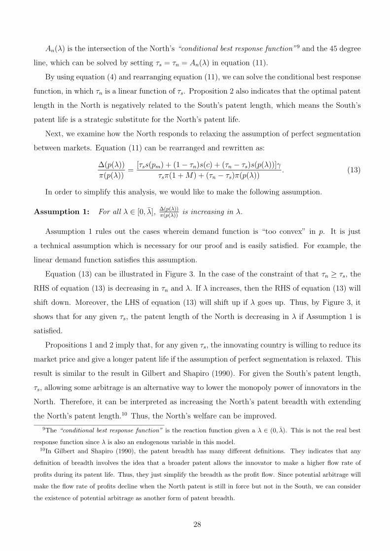
between markets. Equation (11) can be rearranged and rewritten as:

∆(p(λ))

π(p(λ))=

[τss(pm) + (1− τn)s(c) + (τn − τs)s(p(λ))]γ

τsπ(1 + M) + (τn − τs)π(p(λ)). (13)

In order to simplify this analysis, we would like to make the following assumption.

Assumption 1: For all λ ∈ [0, λ], ∆(p(λ))π(p(λ))

is increasing in λ.

Assumption 1 rules out the cases wherein demand function is “too convex” in p. It is just

a technical assumption which is necessary for our proof and is easily satisfied. For example, the

linear demand function satisfies this assumption.

Equation (13) can be illustrated in Figure 3. In the case of the constraint of that τn ≥ τs, the

RHS of equation (13) is decreasing in τn and λ. If λ increases, then the RHS of equation (13) will

shift down. Moreover, the LHS of equation (13) will shift up if λ goes up. Thus, by Figure 3, it

shows that for any given τs, the patent length of the North is decreasing in λ if Assumption 1 is

satisfied.

Propositions 1 and 2 imply that, for any given τs, the innovating country is willing to reduce its

market price and give a longer patent life if the assumption of perfect segmentation is relaxed. This

result is similar to the result in Gilbert and Shapiro (1990). For given the South’s patent length,

τs, allowing some arbitrage is an alternative way to lower the monopoly power of innovators in the

North. Therefore, it can be interpreted as increasing the North’s patent breadth with extending

the North’s patent length.10 Thus, the North’s welfare can be improved.

9The “conditional best response function” is the reaction function given a λ ∈ (0, λ). This is not the real best

response function since λ is also an endogenous variable in this model.10In Gilbert and Shapiro (1990), the patent breadth has many different definitions. They indicates that any

definition of breadth involves the idea that a broader patent allows the innovator to make a higher flow rate of

profits during its patent life. Thus, they just simplify the breadth as the profit flow. Since potential arbitrage will

make the flow rate of profits decline when the North patent is still in force but not in the South, we can consider

the existence of potential arbitrage as another form of patent breadth.

28

τn

LHS

RHS

(λ)

(λ)

(λ)(λ)'

'

RHS LHS

Figure 3: Right hand side (RHS) and left hand side (LHS) of equation (16) where λ′ > λ.

29

We will next examine how the conditional best response function of the South is affected by

the existence of arbitrage. If an interior solution exists, equation (9) can be rewritten as

∆(pm) + π(pm) = (τss(pm) + (1− τs)s(c))(π(1 + M)− π(p(λ)))γ

(1 + M)τsπ(pm) + (τn − τs)π(p(λ)). (14)

Similar to equation (11), the LHS of equation (14) is the marginal social deadweight loss that

the South will incur if it increases its patent length. The RHS of equation (14) is the marginal

social benefit from the additional patent extension.

Equation (14) illustrates a trade-off for the South between dynamic welfare gain and static

efficiency losses similar to that for the North. However, there are two differences between equations

(11) and (14). The first is that the static welfare cost of increasing patent protection in the South

has an effect similar to raising its term of trade, which includes the monopoly profit and the

social deadweight loss, since its domestic price increases. The static welfare cost of extending

patent protection in the North contains an additional effect; the social deadweight loss due to the

monopoly power and enforcement level.

The second difference is that the extension of patent protection in the North will just raise the

profits of the new products in the Northern market with arbitrage. An increase in the South’s

patent life will make an impact on the profits of innovation in both the South and the North

without arbitrage. Thus, the change in the South’s patent protection still could have a large

impact on innovation even though the South is a very small market.

Based on equation (14), we have the following results:

Proposition 3: If τn ≥ As(λ) = γs(c)

(∆(pm)+π(pm))γ+(∆(p(λ))+π(p(λ)))(1+M)π(pm)

(1+M)π(pm)−π(p(λ))

, then the South’s optimal

choice of patent length on [0, τn] is

τs = Max{0,γs(c)− [π(p(λ))(π(pm)+∆(pm))

(1+M)π(pm)−π(p(λ))]τn

(1 + γ)(∆(pm) + π(pm))}. (15)

As(λ) can be solved by letting τn = τs = As(λ) in equation (14). The conditional best response

function, equation (15), can also be derived from the first order condition, which shows that the

optimal patent length in the South is also negatively related to the Northern patent length. This

means the two patent lengths are strategic substitutes for each other.

Next, we will examine the existence of a Nash equilibrium in this non-cooperative patent-

setting game between the North and the South. In Proposition 2 and Proposition 3, we derive the

conditional best response function of the North and South, in the case of τn ≥ τs. It should be

noted that these results will not be sufficient to establish that this pair is a Nash equilibrium. It

30

is only shown that these patent lives are a best response for the North on [τs, 1] and for the South

on [0, τn]. We, therefore, need to show that the North has no incentive to undercut its patent life

and the South will not set τs ∈ [τn, 1].

We prove the existence of a Nash equilibrium by the following lemmas:

Lemma 1: If the demand curve is linear, the Southern market size M is smaller than one, and γ

is constant, there exists a unique pair (τn, τs) satisfying equations (12) and (15) with τn ≥ An(λ)

and τs ≤ As(λ).

The proofs of all Lemmas are in the Appendix. We can conclude that τn and τs are continuous

functions of λ, respectively. The continuity of τn and τs is important for us to prove the existence

of Nash equilibrium. Thus, we can rewrite (τn, τs) = (τn(λ), τs(λ)).

Lemma 2: If the demand curve is linear, the South’s market size M is smaller than one and

γ is constant, then there does not exist any point of intersection between the two conditional best

response functions which involves τn < τs.

Lemma 2 demonstrates that there cannot exist a Nash equilibrium in which τn < τs.

Lemma 3: If the demand curve is linear, the South’s market size M is smaller than one and γ

is constant, then

(i)∂Wn

∂τn

> 0 for τs ∈ [0, As(λ)],

(ii)∂Ws

∂τs

< 0 for τn ∈ [An(λ), 1].

in the case of τn < τs.

Lemma 3 ensures that the solution in Lemma 1 will be a Nash equilibrium. Therefore, we

obtain the following result.

Proposition 4: If the demand curve is linear, the South’s market size M is smaller than one and

γ is constant, there exists a Nash equilibrium (λ∗, τ ∗n, τ ∗s ) satisfying equations (10), (12), and (15)

in this patent-setting game.

Lemma 1 shows that, for any given λ ∈ [0, λ], there exists a unique solution for the two

conditional best response functions, denoted (τn(λ), τs(λ)), while imposing the constraint that

31

τn ≥ τs, in which τn(λ) and τs(λ) are continuous in λ. Next, we need to show that there exists a

λ∗ which maximizes the social welfare of the North.

First, we show that there does not exist a corner solution in this problem. According Proposition

1 and Figure 2, we obtain that ∂Wn(τn(λ∗),τs(λ∗),λ∗)∂λ

> 0 when λ = 0 and ∂Wn(τn(λ∗),τs(λ∗),λ∗)∂λ

< 0 when

λ = λ. Thus, there does not exist any corner solution in this problem.

Next, we need to show that there exists a λ∗ such that

∂Wn(τn(λ∗), τs(λ∗), λ∗)

∂λ= 0.

We rearrange equation (7) and rewrite it as

∆′(p(λ))

π′(p(λ))=

[τss(pm) + (1− τn)s(c) + (τn − τs)s(p(λ))]γ

τsπ(1 + M) + (τn − τs)π(p(λ)). (16)

Since τn and τs are continuous functions of λ, this means that the RHS of equation (16) is

continuous in λ. Since ∆′(p(λ) and π′(p(λ)) are also continuous in λ, the LHS of equation (16) is

also continuous in λ for λ ∈ [0, λ). Since the LHS of equation (16) is close to 0 as λ is close to

zero, the LHS is less than the RHS of equation (16). Furthermore, the LHS is approaching infinity

as λ is close to λ but the RHS is not. Thus, by the intermediate value theorem, we can conclude

the existence of λ∗.

Lemma 2 shows that it is impossible for a Nash equilibrium in which τn < τs to exist. Lemma

3 ensures that (τn(λ∗), τs(λ∗), λ∗) is a Nash equilibrium. This completes the proof of Proposition

4.

If we compare the Nash equilibria with complete segmented market and with relaxing the

assumption of complete segmentation, we find that the North will increase the patent protection

as well as the South. However, we do not conclude which country extends longer. In the following

condition, we obtain an unambiguous result.

Corollary: If, in a Nash equilibrium, the North’s optimal patent length is its economic life, (i.e.,

τn = 1), in the case of perfectly segmented markets, then the gap of optimal patent length between

the two markets will be shorter in a Nash equilibrium in the case of markets that are not completely

segmented.

This Corollary follows from Propositions 1, 2, 3 and 4. Suppose that (τ es , τ e

n) is the Nash

equilibrium when λ ≥ λ. It is hypothesized that τ es < 1 and τ e

n = 1. If the assumption of perfect

segmentation is relaxed, Proposition 4 indicates that there exists a Nash equilibrium , (τ ∗s , τ ∗n, λ∗).

32

By Proposition 1, it implies that λ∗ < λ. Thus, Proposition 2 demonstrates that the conditional

best response function of the North will shift up and Proposition 3 indicates that the conditional

best response function of the South will shift to the right. Therefore, it is easy to show that τ ∗s is

greater than τ es and τ ∗n ≤ 1. This completes the proof of the Corollary.

Efficient International Agreements

The Nash equilibrium outcome can be compared with the efficient agreement that would be chosen

if the policies were chosen to maximize the sum of the North and the South welfare. Such an

outcome would arise if the North and the South were able to commit to an agreement on patent

lives, with lump sum transfers being made between countries to achieve the desired distribution

of the income between countries. In the following, we will examine how total welfare is affected

by the potential for arbitrage if the markets are not perfectly segmented. We will show that

harmonization will never achieve global efficiency in this model.

We prove our argument by a two-step approach. First, like equation (7), we will show that

the globally socially optimal λ will be smaller than λ. This means that relaxing enforcement away

from perfect enforcement will improve global efficiency. Next, we will show that, for any given λ

and N , increasing τn and reducing τs will improve the global welfare.

Since there are only two countries in this economy, the world welfare is sum of the North and

South welfare. Thus, combining equations (2) and (3), we obtain the world welfare function

W (τn, τs, λ, N(τn, τs, λ)) = Wn + Ws

= (τs(1 + M)π(pm) + (τn − τs)π(p(λ)))N + (τss(pm) + (1− τn)s(c)

+ (τn − τs)s(p(λ)))N + M(τss(pm) + (1− τs)s(c))N − C(N). (17)

In order to maximize total welfare, the central planner can choose three variables, λ, τn, and

τs. Taking the derivative with respect to λ, we obtain the following

(τn − τs)(π′(λ) + s′(p(λ)))p′(λ)N

+(τss(pm) + (1− τn)s(c) + (τn − τs)s(λ))(τn − τs)π

′(p(λ))p′(λ)γ

Π. (18)

Similar to equation (7), since π′(pm) is zero and s′(pm) is positive, equation (18) is positive

when λ = λ (and thus the market price is pm). This means that the optimal λ < λ (and so the

optimal p is smaller than pm).

33

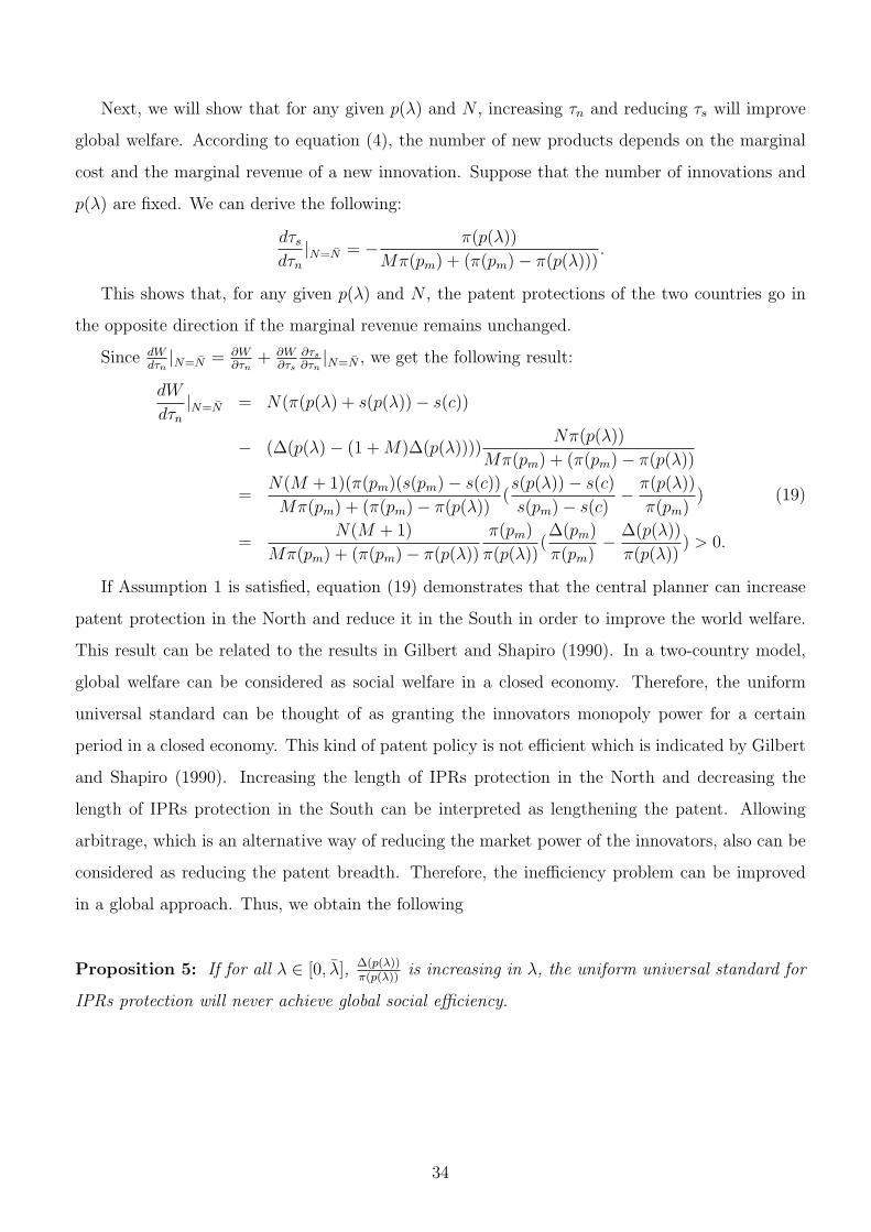
Next, we will show that for any given p(λ) and N , increasing τn and reducing τs will improve

global welfare. According to equation (4), the number of new products depends on the marginal

cost and the marginal revenue of a new innovation. Suppose that the number of innovations and

p(λ) are fixed. We can derive the following:

dτs

dτn

|N=N = − π(p(λ))

Mπ(pm) + (π(pm)− π(p(λ))).

This shows that, for any given p(λ) and N , the patent protections of the two countries go in

the opposite direction if the marginal revenue remains unchanged.

Since dWdτn|N=N = ∂W

∂τn+ ∂W

∂τs

∂τs

∂τn|N=N , we get the following result:

dW

dτn

|N=N = N(π(p(λ) + s(p(λ))− s(c))

− (∆(p(λ)− (1 + M)∆(p(λ))))Nπ(p(λ))

Mπ(pm) + (π(pm)− π(p(λ))

=N(M + 1)(π(pm)(s(pm)− s(c))

Mπ(pm) + (π(pm)− π(p(λ))(s(p(λ))− s(c)

s(pm)− s(c)− π(p(λ))

π(pm)) (19)

=N(M + 1)

Mπ(pm) + (π(pm)− π(p(λ))

π(pm)

π(p(λ))(∆(pm)

π(pm)− ∆(p(λ))

π(p(λ))) > 0.

If Assumption 1 is satisfied, equation (19) demonstrates that the central planner can increase

patent protection in the North and reduce it in the South in order to improve the world welfare.

This result can be related to the results in Gilbert and Shapiro (1990). In a two-country model,

global welfare can be considered as social welfare in a closed economy. Therefore, the uniform

universal standard can be thought of as granting the innovators monopoly power for a certain

period in a closed economy. This kind of patent policy is not efficient which is indicated by Gilbert

and Shapiro (1990). Increasing the length of IPRs protection in the North and decreasing the

length of IPRs protection in the South can be interpreted as lengthening the patent. Allowing

arbitrage, which is an alternative way of reducing the market power of the innovators, also can be

considered as reducing the patent breadth. Therefore, the inefficiency problem can be improved

in a global approach. Thus, we obtain the following

Proposition 5: If for all λ ∈ [0, λ], ∆(p(λ))π(p(λ))

is increasing in λ, the uniform universal standard for

IPRs protection will never achieve global social efficiency.

34

Conclusions

We have developed a simple two-country model of IPRs protection, in which the assumption of

market segmentation is relaxed. This paper examines how arbitrage affects the setting of patent

policy in innovating and non-innovating countries. When patent lives are set non-cooperatively,

it is surprising that the innovating country will not completely eliminate arbitrage, even though

enforcement is costless. The reason is because granting the innovators monopoly power is not

an efficient way to reward innovators. The existence of arbitrage can lower the market price and

improve the innovating country welfare. The innovating country can strengthen the length of IPRs

protection to achieve the maximal welfare. The results are analogous to the results in Gilbert and

Shapiro (1990).

There exists a Nash equilibrium in this patent setting game. It is also shown that the innovating

countries will offer a stronger IPRs protection than non-innovating countries when arbitrage is

possible. Finally, we prove that a uniform universal standard for patent protection will never

achieve global social efficiency.

Appendix

Proof of Lemma 1: Lemma 1 can be proven using Figure 4. First, we need to show that

An(λ) > As(λ). Let Bn(τs) be the best response function for the North, which is defined by

equation (12) in Proposition 2. As in Proposition 2, Bn(τs) is a non-decreasing , continuous, and

piecewise linear function on [0, An(λ)] .

An(λ) is defined as the intersection of Bn(τs) and the 45 degree line, i.e. Bn(τs) = τs. By

equation (8), we can get:

∆(An(λ))(τn(1 + M)π(pm)) = (τns(pm) + (1− τn)s(c))π(An(λ))γ. (20)

By equation (9), it yields:

(∆(pm) + π(pm))τs(1 + Ms)π(pm)

= (τss(pm) + (1− τs)s(c))((1 + M)π(pm)− π(As(λ)))γ. (21)

Let F (τ) = (τs(pm)+(1−τ)s(c))γτ(1+M)π(pm)

, and we can get:

F (An(λ)) =∆(p(An(λ)))

π(p(An(λ)))<

1

2. (22)

35

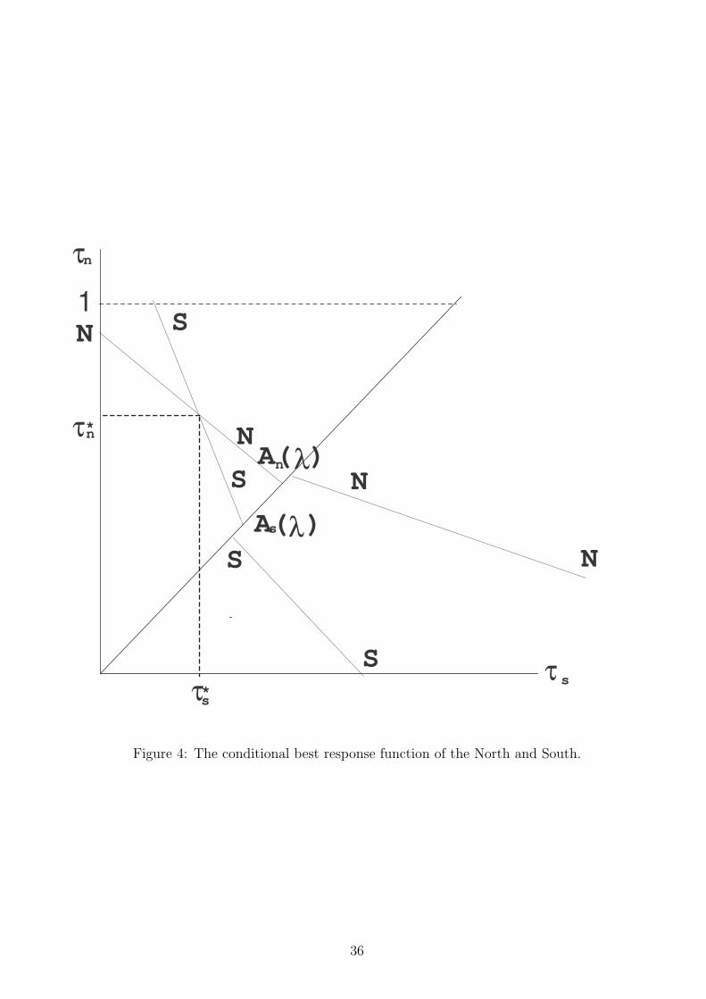
τ

τ

s

n

S

S

N

N

τ

τ

s

n

*

*

1

S

S N

N

A( )λ

n

s

A( )λ

Figure 4: The conditional best response function of the North and South.

36

Since ∆π

= 12

if the demand is linear and M is less than 1, and we can get:

F (As(λ)) =∆(pm) + π(pm)

(1 + M)π(pm)− π(As(λ))>

∆(pm) + π(pm)

(1 + M)π(pm)>

3

4. (23)

Referring to the definitions of An(λ) and As(λ) in Propositions 2 and 3, it can be shown

that An(λ) > As(λ) if and only if F (As(λ)) > F (An(λ)). Therefore, we can conclude that the

intersection of the North’s reaction function and the 45 degree line, An(p(λ)), is to the right of

the intersection of the South’s reaction functions and the 45 degree line, As(p(λ)), under the

assumptions of Lemma 1 and the constraint τn ≥ τs.

We will now show that there exists a unique solution satisfying equations (12) and (15), using

the following five cases.

Case 1: If As(λ) ≥ 1, which means An(λ) > 1. Since Bn(τs) = 1 for all τs ∈ [0, 1] and Bs(τn) = 1

for all τn ∈ [0, 1], the only solution is (1, 1).

Let a “-” over a variable denote the maximum value of that variable and a “-” under a variable

denote the minimum value of that variable.

Case 2: If As(λ) < 1, Bs(1) > 0, and B−1n (1) ≥ Bs(1). Since An(λ) > As(λ), B−1

n (τn) is greater

than Bs(τn) for all τn ∈ [An(λ), 1). Additionally, Bn(τs) = 1 for all τs ∈ [0, B−1n (1)). Therefore,

the unique solution is (1, Bs(1)).

Case 3: If As(λ) < 1, Bs(1) > 0 and B−1n (1) < Bs(1). Since B−1

n (1) < Bs(1), there is no solution

for all τs ∈ [0, B−1s (1)]. Bn(τs) is a linear, decreasing function in τs. Therefore, B−1

s (.) − Bn(.) is

positive when τs = Bs(1) because B−1s (Bs(1)) = 1 and Bn(Bs(1)) < 1. Furthermore, B−1

s (.)−Bn(.)

is negative when τs = As(λ) because B−1s (Bs(As(λ))) = As(λ) < An(λ) = Bn(An(λ)) < Bn(As(λ)).

By continuity, we can conclude that there exists a pair of (τn, τs) satisfying 1 > τn > An(λ) and

0 < τs < As(λ).

Case 4: If As(λ) < 1, Bs(1) = 0 and Bn(0) ≥ B−1s (0). Bn(τs) is greater than B−1

s (τs) for

all τs ∈ (0, As(λ)]. Also, Bs(τn) = 1 for all τn ∈ [B−1s (0), 1]. Therefore, the unique solution is

(Bn(0), 0).

Case 5: If As(λ) < 1, Bs(1) = 0 and Bn(0) < B−1s (0). Since Bn(0) < B−1

s (0), there is

no solution for τs = 0. Since Bs(τn) is a linear, decreasing function in τn, Bs(τn) > 0 for all

τn ∈ (B−1s (0), As(λ)]. Therefore, B−1

n (.) − Bs(.) is negative when τn = Bn(0). This is because

B−1n (Bn(0)) = 0 and Bs(Bn(0)) > Bs(B

−1s (0)) = 0. Furthermore, B−1

n (.) − Bs(.) is positive when

τn = An(λ) because B−1n (Bn(An(λ))) = An(λ) > As(λ) = Bs(As(λ)) > Bs(An(λ)). By continuity,

37

we can conclude that there exists a pair of (τn, τs) satisfying 1 > τn > An(λ) and 0 < τs < As(λ).

This completes the proof of Lemma 1.

Proof of Lemma 2:

To prove Lemma 2, we first show that the intersection point of the North’s conditional best

response function and the 45 degree line is to the right of the intersection point of the South’s con-

ditional best response function and the 45 degree line in the case of τn < τs. We then demonstrate

the slope of the North’s best response function of the North is flatter than the South’s.

Since patent protection is longer in the South, arbitrage will potentially occur there. This

changes the profit function, the welfare functions, and the social surplus. We will redefine most of

the equations in sections 2 and 3.

First, the profit function Π is:

Π(τs, τn, λs, N) = τn(1 + M)π(pm) + M(τs − τn)π(ps(λs)). (24)

Total differentiating C(N∗) = Π(τs, τn, λs, N∗) yields:

dN∗

N∗ = [(π + M(π − π(ps)))dτn + Mπ(ps)dτs + (τs − τn)Mπ′(p(λs))p′(λs)dλs]

γ

Π,

Similar to equations (2) and (3), the welfare functions can be rewritten as:

Wn(τn, τs, λs, N∗(τs, τn, λs)) = (τn(1 + M)π + M(τs − τn)π(ps(λs)))N

∗

+ N∗(τns(pm) + (1− τn)s(c))− C(N∗), (25)

and

Ws(τn, τs, λs, N∗(τs, τn, λs)) = N∗M(τns(pm) + (τs − τn)s(ps(λs)) + (1− τs)s(c)). (26)

Differentiating equation (25) with respect to τn, we obtain the following first order condition:

∂Wn

∂τn

= N∗(−∆ + M(π − π(ps(λs))))

+ (τns(pm) + (1− τn)s(c))(π + M(π − π(ps(λs))))N∗γΠ

= 0. (27)

Again, taking the derivative of equation (26) with respect to λs, τs, we obtain the following

first order conditions:

∂Ws

∂τs

= N(s(ps(λs))− s(c))

+ [(τns(pm) + (τs − τn)s(ps(λs)) + (1− τs)s(c))Mπ(ps(λs))]N∗γΠ

= 0, (28)

38

and

∂Ws

∂λs

= N∗s′(ps(λs))(τs − τn) + [(τns(pm) + (τs − τn)s(ps(λs))

+ (1− τs)s(c))]N∗γ(τs − τn)Mπ′(ps(λs))p

′s(λs)

Π= 0. (29)

Equation (29) shows that the South also will not eliminate all arbitrage that occurs there. The

reason is the same as the North’s, which we indicated in Proposition 1.

Next, we examine the conditional best response function of the North when τn is equal to τs.

According to the first conditions of equations (27) and (28), the conditional best response functions

should satisfy the following conditions if the interior solution is available:

(∆−M(π − π(ps(λs))))(τn(1 + M)π)

= (τns(pm) + (1− τn)s(c))(π + M(π − π(ps(λs))))γ,

and,

(s(c)− s(ps(λs)))(τs(1 + M)π) = (τss(pm) + (1− τs)s(c))Mπ(ps(λs))γ

Letting F (τ) = (τs(pm)+(1−τ)s(c))γτ(1+M)π

, we get:

F (τn) =(∆−M(π − π(ps(λs))))

π + M(π − π(ps(λs)))<

1

2< 1 <

1

M<

s(c)− s(ps(λs))

Mπ(ps(λs))= F (τs), (30)

Since F (.) is a decreasing function in τ , equation (30) indicates that that the intersection point

of the North’s conditional best response function and the 45 degree line is to the right of the

intersection point of the South’s conditional best response function and the 45 degree line.

Next, we show that the slope of the North’s conditional best response function is flatter than the

South’s. Differentiating equation (28) with respect to τn and τs yields the slope of the conditional

best response function of the South:

dτn

dτs

|S = − (s(c)− s(ps(λs)))Mπ(ps(λs))(1 + γ)

(s(c)− s(ps(λs)))[π + M(π − π(ps(λs)))] + (s(ps(λs))− s(pm))Mπ(ps(λs))γ.

Differentiating equation (27) with respect to τn and τs yields the slope of the North’s “best

response function”:

dτn

dτs

|N = − Mπ(ps(λs))(∆−M(π − π(ps(λs))))

[π + M(π − π(ps(λs)))][γ(π + ∆) + ∆−M(π − π(ps(λs)))].

Let Q = π − π(ps(λs)). If ∆−MQ < 0, there is no best response function for the North since

∂Wn

∂τn> 0. If ∆−MQ > 0, we need to show

(1 + γ)

[π + MQ] + (s(ps(λs))− s(pm))M π(ps(λs))s(c)−s(ps(λs))

γ>

(∆−MQ)

[π + MQ][γ(π + ∆) + ∆−MQ)],

39

Since (1+γ)

[π+MQ]+(s(ps(λs))−s(pm))Mπ(ps(λs))

s(c)−s(ps(λs))γ

> (1+γ)[π+MQ]+(s(ps(λs))−s(pm))Mγ

> (1+γ)[π+MQ]+(π+∆)Mγ

, it suf-

fices to show

(1 + γ)

[π + MQ] + (π + ∆)Mγ>

(∆−MQ)

[π + MQ][γ(π + ∆) + ∆−MQ]

Since γππ > γMπ∆ and γ∆π > γM∆2, we yield

(1 + γ)[π + MQ][γ(π + ∆) + ∆−MQ] = (∆−MQ)[π + MQ] + γ(∆−MQ)[π + MQ]

+γππ + γπMQ + γ∆π + γ∆MQ + γ2(π + ∆)[π + MQ]

> (∆−MQ)[π + MQ] + (∆−MQ)(π + ∆)Mγ = ([π + MQ] + (π + ∆)Mγ)(∆−MQ)

This completes the proof of Lemma 2.

Proof of Lemma 3:

(i) is proven by a two-step approach. First, we show that the intersection of the Northern

reaction function and the 45 degree line is to the right of As(λ). We, then, show that ∂Wn

∂τn> 0

for τs ∈ [0, As(λ)]. Equations (23) and (30) proves this. Equation (27) shows that for any (τn, τs)

below the conditional best response function of North, ∂Wn

∂τnis positive. This completes the proof

of (i).

The proof of (ii) is analogous to (i). Equations (22) and (30) show that the intersection of

the Southern conditional best response function and the 45 degree line is to the left of An(λ).

Equation (28) shows that for any point above the conditional best response function of South, ∂Ws

∂τs

is negative. This completes the proof of (ii).

40

References

Braga, C.P. (1990), “The Developing Country Case for and against Intellectual Property Protec-

tion,” in Siebeck, W.E.(Eds), Strengthening Protection of Intellectual Property in Developing

Countries: A Survey of the Literature. World Bank Discussion Paper, no. 112.

Chin, Judith C. and Gene M. Grossman (1990), “Intellectual Property Rights and North-South

Trade,” in Jones R., Krueger, A.O.(Eds), The Political Economy of International Trade,

Cambridge, MA: Basil Blackwell, 90-107.

Deardorff, Alan V. (1992), “Welfare Effects of Global Patent Protection,” Economica, 59, 35-51.

Diwan, Ishak and Dani Rodrik (1991), “Patents, Appropriate Technology, and North-South

Trade,” Journal of International Economics, 23, 79-90.

The Economist (1996), “Stolen Melodies,” May 11; 339, 64.

Gallini, Nancy T., and Suzanne Scotchmer (2002), “Intellectual Property: When Is It the Best

Incentive System?” Innovation Policy and the Economy, Vol 2, Adam Jaffe, Joshua Lerner

and Scott Stern, eds, MIT Press, 51-78.

Gilbert, Richard and Carl Shapiro (1990), “Optimal Patent Length and Breadth,” RAND Journal

of Economics, 21, 106-112.

Grossman, Gene M. and Elhanan Helpmam (1994), “Protection for Sale,” American Economic

Review, 84, 833-850.

Grossman, Gene M. and Edwin L.C. Lai (2004), “International Protection of Intellectual Prop-

erty,” American Economic Review, 94, 1635-1653.

Krugman, Paul R. (1992), “Regionalism versus Multilateralism,” in J. De Melo and A. Panagarya,

eds. New Dimensions in Regional Integration. Cambridge University Press, 58-79.

Lai, Edwin L.C. and Larry D. Qiu (2003), “The North’s Intellectual Property Rights Standard

for the South?” Journal of International Economics, 59, 183-209.

Maskus Keith E., (2000), Intellectual Property Rights in the Global Economy, Washington, DC:

Institute for International Economics.

41

Mitra, Devashish (1999), “Endogenous Lobby Formation and Endogenous Protection: A Long-

Run Model of Trade Policy Determination,” American Economic Review, 89, 1116-1134.

Nordhaus, William D. (1969), Invention, Growth, and Welfare: A Theoretical Treatment of Tech-

nological Change, Cambridge, Mass., M.I.T. Press.

Scherer, Frederic M. (1980), Industrial Market Structure and Economic Performance, Chicago:

Rand McNally College Pub. Co.

Scotchmer, Suzanne (2004), “The Political Economy of Intellectual Property Treaties,” Journal

of Law, Economics, and Organizations, 20, 415-437.

Spors, Kelly K. (2004), “Canadian Drugs Are Getting Cheaper; Online Pharmacies Catering to

American Cut Costs by Finding New Surppliers,” Wall Street Journal, July 22.

State Legislatures (2004), “Canadian Drugs: Panacea or Problem?” June; 30, 6.

Weil, Elizabeth (2004), “Grumpy Old Drug Smugglers,” New York Times Magazine, May 30,

42-45.

42

CHAPTER IV

WHY DOES THE U.S. PREVENT PARALLEL IMPORTS?

Introduction

Parallel imports, also called “gray-market imports,” are authorized for their first sale, not coun-

terfeited or pirated, but imported by unauthorized resellers. Those commodities are identical to

legitimate products except that they may be packaged differently and may not carry the orig-

inal manufacturer’s warranty. It occurs when one manufacturer owns the patents or national

trademarks in several countries. In order to make its maximal profits, the manufacturers would

rationally grant low prices in low-income countries or in the markets with elastic demand and set

high prices in high-income countries or in less-elastic-demand markets.

One of the most important issues of parallel trade is the welfare effects. Varian (1985) and

Malueg and Schwartz (1994) indicate that parallel trade would result in uniform pricing interna-

tionally and would reduce global welfare because parallel trade could make some markets unserved.

Maskus and Chen (2002, 2004) develop a model of parallel trade and vertical price control in which

a manufacturer sells aboard through a retailer and tries to achieve the profit-maximizing price by

setting its wholesale price and licence fee. It concluded that banning parallel trade is always benefi-

cial to the monopolist producer, but could raise or reduce global surplus. Chen and Maskus (2005)

generalize the results of Maskus and Chen (2004) and find that open parallel trading regimes

may improve welfare within regional trade agreement. Richardson (2002) indicates that, in a

Nash equilibrium, no importing countries would not permit parallel importing because they are

discriminated against in its absence.

The existing literature on parallel trade always conclude that the welfare of importing country

is seemingly improved because the price of parallel imports decreases. However, there exists the

phenomenon that some developed countries, such as the U.S., do not like to permit parallel imports.

For example, we can easily find the following messages in international edition textbook: “This

International Edition is not for sale in the United States of America, its dependencies or Canada.”1

This message or similar statements usually appear on the copy right page of the International

1See Nicholson (1985).

43

Edition textbook.2 This indicates that the U.S. does not allow the international edition textbooks

to circulate in the U.S. and Canada; this is true ever for used books.3

Policy toward parallel trade varies worldwide. In general, policies can be divided into three

categories, national exhaustion, regional exhaustion, and international exhaustion. National ex-

haustion means that intellectual property rights (IPRs) end upon original sale within a nation but

IPRs owners may prevent parallel trade with other countries. International exhaustion means that

IPRs are exhausted upon original sale and parallel trade is permitted. Regional exhaustion means

that IPRs are completed within a group of countries, allowing parallel trade among them, but are

not exhausted outside the region.

Some countries’ policies are summarized in Table 1. It shows that Japan permits parallel

imports unless they are barred by contract or its original sale is regulated by price-control. Thus,

we conclude that Japan is regularly open for parallel trade. Moreover, the European Union policy

is regional exhaustion. It also shows that the U.S. policy is generally national exhaustion. The U.S.

policy permits trademark owners to block parallel imports with some exceptions, such as when

both the foreign and the U.S. companies belong to the same entity or when the foreign and the

U.S. companies are in a parent-subsidiary relationship, which means the U.S. significantly restricts

parallel trade. Therefore, parallel trade in the U.S. is more restrictive than in other developed

countries.

In this paper, we would like to ask: What is the reason for the difference between U.S. and

Japanese policy? If parallel importing is always in favor of the importing country, it is difficult to

explain why the U.S. would not like to allow parallel importing. Most of the existing literature on

parallel trade (i.e. Malueg and Schwartz (1994), Maskus and Chen (2002, 2004), Chen and Maskus

(2005)) usually employed a single product model to demonstrate how parallel trade impacts welfare.

To date, to the best of my knowledge, no paper discusses how parallel trade affects the incentives of

innovation. Furthermore, most papers on parallel trade use the global welfare approach to explain

why some countries prevent parallel trade, which I think that is unreasonable. They do not explain

by the viewpoint of importing country.

The purpose of this paper is to propose a simple two-country model with innovation to analyze

the welfare effects of parallel imports. We try to use this model to explain why some of the

2In McGraw-Hill international edition textbook, the following statement, “This book cannot be re-exported from

the country to which it is consigned by McGraw-Hill.,” appears.3For example, we can not sell the international edition used books on www.amazon.com, ebay.half.com or other

similar websites.

44

Tab

le1:

Sum

mar

yof

IPR

Exhau

stio

nR

egim

es.

Cou

ntr

yTra

dem

arks

Pat

ents

Cop

yri

ghts

Euro

pea

nU

nio

nC

omm

unity

exhau

stio

nC

omm

unity

exhau

stio

nC

omm

unity

exhau

stio

n

USA

Nat

ional

exhau

stio

nlim

ited

by

com

-

mon

contr

olan

dno

consu

mer

confu

-

sion

Nat

ional

exhau

stio

nN

atio

nal

exhau

stio

n

Jap

anIn

tern

atio

nal

exhau

stio

nunle

ss

agre

edby

contr

act

oror

igin

alsa

leis

pri

ce-c

ontr

olle

d

Sam

eas

trad

emar

ks

Sam

eas

trad

emar

ks

Aust

ralia

Inte

rnat

ional

exhau

stio

nN

atio

nal

exhau

stio

nunle

ssso

ldby

pat

ent

owner

wit

hou

tcl

ear

rest

ric-

tion

s

Nat

ional

exhau

stio

nex

cepti

onfo

r

com

pac

tdis

csan

dbook

s

Sou

rces

:M

askus

(200

0a)

45

developed countries, such as the U.S., will not allow parallel imports. We utilize a simulation

approach to investigate the welfare effects of parallel trade on the importing country and global

welfare.

The remainder of this paper is organized as follows: In section 2, we demonstrate that the

welfare of the importing country improves in a conventional two-country model with linear demand.

In section 3, we set up a two-country model of parallel trade, in which innovation is incorporated.

We employ a simulation approach to explain why the U.S. does not allow parallel imports. Section

4 gives conclusions.

The Single Product Case

In this section, we describe a simple, conventional, two-country model of parallel trade with a single

product. Consider an economy in which there are two countries, North and South, denoted n and

s, and a monopolistic manufacturer. The monopolist manufacturer produces and sells identical

products in both countries.

The inverse demand function in market i is

pi(qi) = ai(1− qi), i = n, s. (1)

where pi and qi is the price and consumption in country i, respectively.4 This kind of linear demand

function has equal horizontal intercept, at 1, but different vertical intercepts, ai. Furthermore, we

assume that an = 1 + x and as = 1− x, where x < 1.

The monopolist determines the price in both markets to maximize its profits. Suppose that the

markets are segmented. The producer can price discriminate in the two countries so as to make its

maximal profit. This is third degree price discrimination. This means that the producer can set

different prices in different markets according the demand elasticity of market. Suppose that the

marginal production cost is constant and the same in the two countries. For simplicity, I assume

that marginal production cost is zero, without loss of generality. Therefore, the monopoly price

in the North, pmn = 1+x

2, would be higher than the price in the South’s market, pm

s = 1−x2

, which

implies that the North is the importing country if parallel trade exists.

Since there exists a price difference, there exist incentives for arbitrage. Parallel imports are

brought into the North from the South. For simplicity, we assume that there is no transaction

4The specification of this linear demand function follows Malueg and Schwartz (1994).

46

cost. Since arbitrage is unlimited, the market of the parallel imports in the North is competitive.5

Therefore, the optimization problem of the monopolist is to choose the price p to maximize

π(p) = p[(1− p

1 + x) + (1− p

1− x)], (2)

where p is the uniform price, (1− p1+x

) and (1− p1−x

) are the consumptions in the North and the

South, respectively.

The monopolist chooses the uniform price p to maximize its profit. Taking derivative with

respect to p, we obtain the following:

∂π(p)

∂p= 2− 2p

1 + x− 2p

1− x.

The optimal price can be solved by the first order condition. We obtain

p∗ =1− x2

2. (3)

Note that p∗ is greater than pms , but less than pm

n .

Next, we investigate the welfare effects of parallel trade. First, we want to show that parallel

trade will improve global welfare. When the two markets are segmented, we can get that the sum

of consumers’ surplus and producer’s surplus in the North is 3(1+x)8

and 3(1−x)8

for the South. Thus,

we find that the global welfare is 34.

If parallel trade exists, the optimal price, p∗, is 1−x2

2. Thus, the sum of consumers’ surplus and

producer surplus in the North is (1 + x)2(3− x)/8 and (1− x)2(3 + x)/8 in the South. Therefore,

global welfare is 34+ x2

4. Thus, we can conclude that the global welfare in the case of parallel trade

is greater than in the case of segmented markets. Furthermore, global welfare is increasing in x.

If the monopolist is from the North, the welfare of the South decreases when parallel trade

happens since the price of the product in the South goes up. Thus, the welfare of the North

improves. Moreover, if the monopolist is from the South, it is easy to show that the welfare of

the North improves because the price in the North decreases. Therefore, we obtain the following

conclusions:

Proposition 1: (a) Global welfare is improved by allowing parallel trade. (b) The welfare of

the North increases if parallel trade allowed.

5There exists an alternative approach of analysis in distribution of parallel imports. Maskus and Chen (2002,

2004), and Chen and Maskus (2005) propose a model of duopoly, in which parallel importer and the producer

compete in the importing market. However, we think that similar results for the issue of this paper apply for their

model. Furthermore, unlimited arbitrage and competitive market make this analysis simpler.

47

Proposition 1 indicates that the welfare of importing country improves when the demand func-

tions are linear in the case of a single product model. Actually, Tirole (1988) indicates that when

the demand functions are linear, the welfare of third price discrimination is lower than uniform

pricing. Thus, we can generalize the above linear demand model to different market size and the

results remain the same. Furthermore, we also can conclude that the importing country increases

their welfare by parallel importing in Varian (1985) and Malueg and Schwartz (1994), in which a

multi-country model is employed. For simplicity, we just focus on the case of a two-country model

with the same market size.

In the next section, we investigate the welfare effects of parallel trade in the case of multiple

products and try to explain why some developed countries do not allow parallel imports.

The Welfare Effects of Parallel Trade Incorporated with Innovation

In this section, we develop a two-country model of parallel trade, in which innovation is incor-

porated. Consider an economy with two countries, named South (s) and North (n), and a firm

that develops new products in the North. The model follows Deardorff (1992) and Scotchmer

(2004) by considering a two-stage model of innovation. It is assumed that there are two sectors,

a homogenous good sector and a differentiated products sector. In the first stage, firms choose

the number of differentiated products to be produced and sold in the two markets in the second

period. Individuals are assumed to have identical preferences in their country but the consumers

have different preferences in the South and the North. Each consumer chooses z and x(j) to

maximize his utility which is given by:

∫ N

0ui(xi(j))dj + zi,

subject to∫ N

0pi(j)xi(j)dj + zi = Yi, (4)

where j is the index of differentiated goods, N is the measure of new differentiated products in

the North, xi(j) is the consumption of a differentiated good j in country i, zi is the consumption

of the homogenous good, and Yi is individual income in country i. We assume that u′ > 0 and

u′′ < 0. From the first order conditions, it yields xi(j) = xi(p(j)) where xi = (u′i)−1. The demand

for the numeraire good is given by:

zi = Yi − pi(j)xi(pi(j)).

48

The indirect utility function can be written as:

U =∫ N

0si(pi(j))dj + Yi,

where si(pi(j)) = ui(xi(pi(j)))− pi(j)xi(p(j)) is the consumer surplus associated with a represen-

tative differentiated product, Yi is consumer’s income. The two-stage model can be thought of

as representing the steady state of an infinite horizon general equilibrium model in which firms

innovate in every period and products have an exogenously given useful life, as has been shown by

Grossman and Lai (2004). For the sake of comparison, we assume that the demand function for

each differentiated product is just like equation (1) in a different country.

Suppose that manufacturing requires only labor. Since the homogenous good z is considered

as the numeraire, without loss of generality, we assume that the production of the homogeneous

good z requires one unit of labor per unit of output and the market for z is competitive, which

makes the price of z equal to one. Furthermore, suppose that the production of one unit of all

varieties of differentiated products requires c units of labor. Just like section 2, we assume that c

is equal to zero.

In the following, we employ a simulation approach to investigate the welfare effects of parallel

trade for the North and the global welfare effects.

The innovation cost function is specified as follows:

C(N) = Nα, (5)

where α is greater than one.6 According to equation (5), we know that the innovation cost is

convex in N . We also denote that

γ = C ′(N)/(NC ′′(N))

is the elasticity of innovation with respect to an increase in the profit from innovation, which

follows Grossman and Lai (2004). This specification of innovation cost function has a constant

elasticity of innovation, which has the same properties as the innovation cost function in Grossman

and Lai (2004).

The problem of this firm is to choose the number of the new differentiated products, N , and

the price in both markets to maximize its profit. Since the ps and pn are determined as in Section

6Otherwise, the marginal innovation cost and the average innovation cost are going down, which means that the

number of innovation becomes infinite.

49

2, the optimal N∗ is determined by marginal profit and the marginal innovation cost of innovating

a new differentiated good. Thus,

C ′(N∗) = πn(pn) + πs(ps).

where the right hand side is the marginal profit generated by an additional product.

The welfare of the North is composed of the profit of the firm in the North and the South, the

consumers’ surplus in the North, and the innovation cost.

Wn(N) = N(πn(pn) + πs(ps) + sn(pn))− C(N).

Moreover, since the firm is in the North, the welfare of the South is only the consumers’ surplus

generated in the South.

Ws(N) = Nss(ps).

Furthermore, global welfare is defined as the sum of the welfare of the North and the South,

i.e. W = Wn + Ws.

We examine the welfare effects of parallel trade by numerical simulation for x ∈ [0, 0.5] for

different innovation cost functions.7 Since we obtain similar results for different cases of the

innovation cost function, we just illustrate two cases of γ in Figure 1 and Figure 2. In Figure 1 and

Figure 2, the x-axis is defined as x and the y-axis is defined as the relative welfare of the North

and relative global welfare, .

Two cases of elasticity of innovation, γ = 5 and γ = 1011

are illustrated in Figure 1 and Figure

2, respectively. The former represents the cases of high elasticity of innovation and the latter

represents the cases of low elasticity of innovation. “Wn ratio” is defined as the North’s welfare

when parallel trade happens divided by the welfare of the North when parallel trade does not exist.

Thus, “Wn ratio” is greater than 1 means that the North’s welfare improves when parallel trade

exists. Analogously, the GW ratio is the global welfare ratio, which is greater than 1 means the

global welfare improves if parallel trade happens.

Figure 1 shows that two North’s welfare is concave in x. It is increasing in x first, and then

decreasing in x. We can find that there exists a x = 0.117, which makes the North obtain the

maximal welfare improvement (Wn ratio) from parallel imports. For x ∈ [0.117, 0.5], the North

welfare is decreasing in x and there exists x = .231 such that the North welfare of parallel trade

is equal the welfare if parallel trade does not exist. This means that if x is big enough, parallel

7Since there will not exist parallel trade for the case of x > 0.5, we just focus on the case of x ∈ [0, 0.5].

50

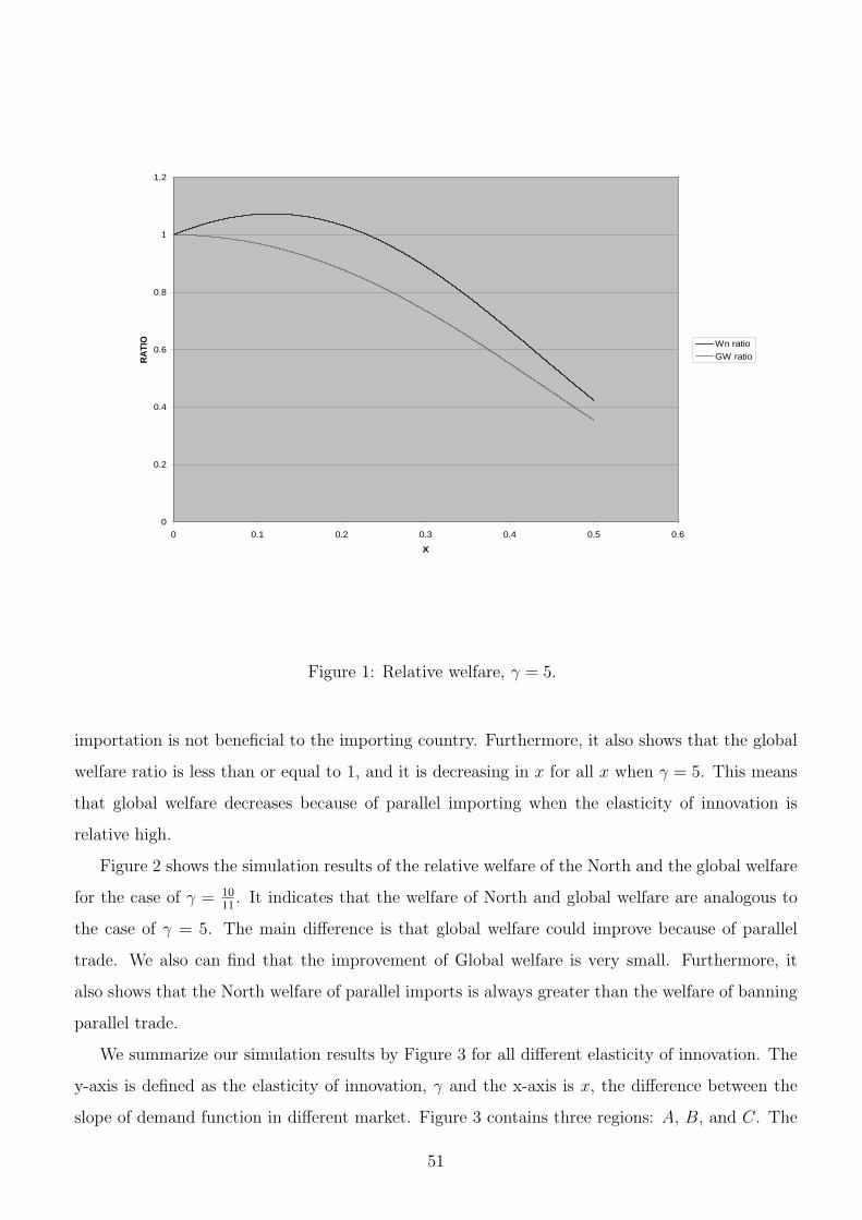
0

0.2

0.4

0.6

0.8

1

1.2

0 0.1 0.2 0.3 0.4 0.5 0.6

X

RA

TIO Wn ratio

GW ratio

Figure 1: Relative welfare, γ = 5.

importation is not beneficial to the importing country. Furthermore, it also shows that the global

welfare ratio is less than or equal to 1, and it is decreasing in x for all x when γ = 5. This means

that global welfare decreases because of parallel importing when the elasticity of innovation is

relative high.

Figure 2 shows the simulation results of the relative welfare of the North and the global welfare

for the case of γ = 1011

. It indicates that the welfare of North and global welfare are analogous to

the case of γ = 5. The main difference is that global welfare could improve because of parallel

trade. We also can find that the improvement of Global welfare is very small. Furthermore, it

also shows that the North welfare of parallel imports is always greater than the welfare of banning

parallel trade.

We summarize our simulation results by Figure 3 for all different elasticity of innovation. The

y-axis is defined as the elasticity of innovation, γ and the x-axis is x, the difference between the

slope of demand function in different market. Figure 3 contains three regions: A, B, and C. The

51

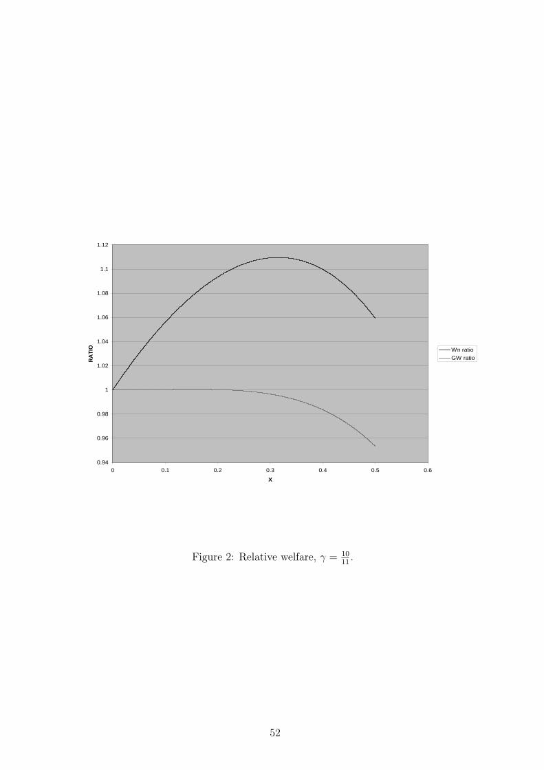
0.94

0.96

0.98

1

1.02

1.04

1.06

1.08

1.1

1.12

0 0.1 0.2 0.3 0.4 0.5 0.6

X

RA

TIO Wn ratio

GW ratio

Figure 2: Relative welfare, γ = 1011

.

52

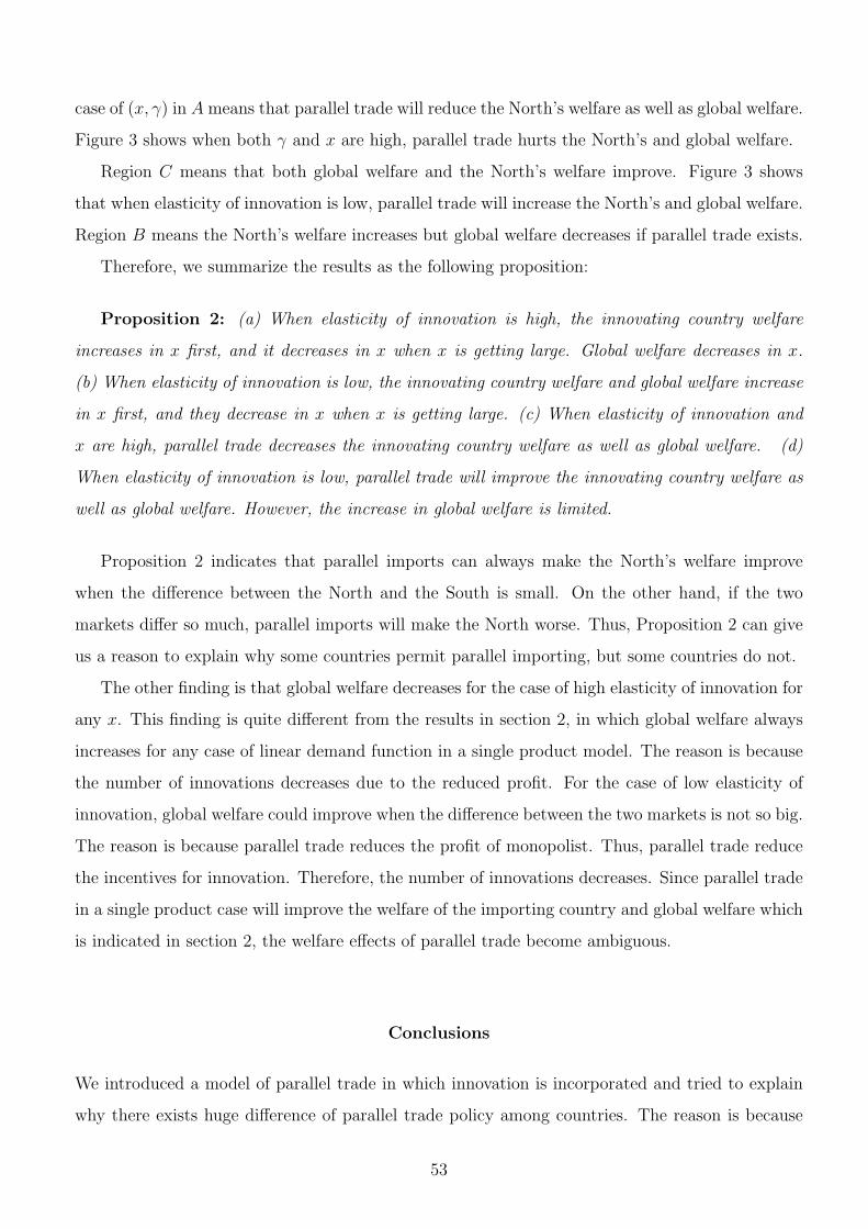
case of (x, γ) in A means that parallel trade will reduce the North’s welfare as well as global welfare.

Figure 3 shows when both γ and x are high, parallel trade hurts the North’s and global welfare.

Region C means that both global welfare and the North’s welfare improve. Figure 3 shows

that when elasticity of innovation is low, parallel trade will increase the North’s and global welfare.

Region B means the North’s welfare increases but global welfare decreases if parallel trade exists.

Therefore, we summarize the results as the following proposition:

Proposition 2: (a) When elasticity of innovation is high, the innovating country welfare

increases in x first, and it decreases in x when x is getting large. Global welfare decreases in x.

(b) When elasticity of innovation is low, the innovating country welfare and global welfare increase

in x first, and they decrease in x when x is getting large. (c) When elasticity of innovation and

x are high, parallel trade decreases the innovating country welfare as well as global welfare. (d)

When elasticity of innovation is low, parallel trade will improve the innovating country welfare as

well as global welfare. However, the increase in global welfare is limited.

Proposition 2 indicates that parallel imports can always make the North’s welfare improve

when the difference between the North and the South is small. On the other hand, if the two

markets differ so much, parallel imports will make the North worse. Thus, Proposition 2 can give

us a reason to explain why some countries permit parallel importing, but some countries do not.

The other finding is that global welfare decreases for the case of high elasticity of innovation for

any x. This finding is quite different from the results in section 2, in which global welfare always

increases for any case of linear demand function in a single product model. The reason is because

the number of innovations decreases due to the reduced profit. For the case of low elasticity of

innovation, global welfare could improve when the difference between the two markets is not so big.

The reason is because parallel trade reduces the profit of monopolist. Thus, parallel trade reduce

the incentives for innovation. Therefore, the number of innovations decreases. Since parallel trade

in a single product case will improve the welfare of the importing country and global welfare which

is indicated in section 2, the welfare effects of parallel trade become ambiguous.

Conclusions

We introduced a model of parallel trade in which innovation is incorporated and tried to explain

why there exists huge difference of parallel trade policy among countries. The reason is because

53

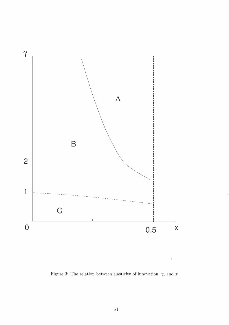
2

1

0 0.5 x

γ

Α

B

C

Figure 3: The relation between elasticity of innovation, γ, and x.

54

if parallel imports are allowed, it will reduce the incentives for innovation of the innovators, then

reduce the number of new innovation. The results show that the welfare effect is not only related to

the difference of the two markets, but is also related to the elasticity of innovation. Parallel trade

improves the welfare of importing country. However, parallel trade also reduces the incentives to

innovate. Thus, the welfare effect of parallel imports is ambiguous. It explains that some countries

parallel import and some do not. Furthermore, we also show that when elasticity of innovation

and x are high, parallel trade decreases the innovating country welfare as well as global welfare.

When elasticity of innovation is low, parallel trade will improve the innovating country welfare as

well as global welfare. However, the increase in global welfare is limited.

55

References

Chen, Yongmin and Keith E. Maskus (2005), “Vertical Pricing and Parallel Imports,” Journal of

International Trade and Economic Development, 14, 1-18.

Deardorff, Alan V. (1992), “Welfare Effects of Global Patent Protection,” Economica, 59, 35-51.

Grossman, Gene M. and Edwin L.C. Lai (2004), “International Protection of Intellectual Prop-

erty,” American Economic Review, 94, 1635-1653.

Malueg, David A. and Marius Schwartz (1994), “Parallel Imports, Demand Dispersion, and In-

ternational Price Discrimination,” Journal of International Economics, 37, 167-195.

Maskus, Keith E. (2000a), Intellectual Property Rights in the Global Economy, Washington, DC:

Institute for International Economics.

Maskus, Keith E. (2000b), “Parallel Imports,” The World Economy, 23, 1269-1284.

Maskus, Keith E. and Yongmin Chen (2002), “Parallel Imports in a Model of Vertical Distribution:

Theory and Evidence and Policy,” Pacific Economic Review, 7, 319-334.

Maskus, Keith E. and Yongmin Chen (2004), “Vertical Price Control and Parallel Imports: The-

ory and Evidence,” Review of International Economic, 12, 551-570.

Nicholson, Walter (1985), Microeconomic Theory, Third Edition, The Dryden Press.

Richardson, Martin (2002), “An Elementary Proposition Concerning Parallel Imports,” Journal

of International Economics, 56, 233-245.

Scotchmer, Suzanne (2004), “The Political Economy of Intellectual Property Treaties,” Journal

of Law, Economics, and Organizations, 20, 415-437.

Tirole, Jean (1988), The Theory of Industrial Organization, Cambridge, MA, The MIT press.

Varian, Hal R. (1985), “Price Discrimination and Social Welfare,” American Economic Review,

75, 870-875.

56