by volodymyr mnih - university of torontovmnih/docs/mnih_volodymyr_phd_thesis.pdf · machine...
TRANSCRIPT

Machine Learning for Aerial Image Labeling
by
Volodymyr Mnih
A thesis submitted in conformity with the requirementsfor the degree of Doctor of Philosophy
Graduate Department of Computer ScienceUniversity of Toronto
c© Copyright 2013 by Volodymyr Mnih

Abstract
Machine Learning for Aerial Image Labeling
Volodymyr Mnih
Doctor of Philosophy
Graduate Department of Computer Science
University of Toronto
2013
Information extracted from aerial photographs has found applications in a wide range
of areas including urban planning, crop and forest management, disaster relief, and
climate modeling. At present, much of the extraction is still performed by human
experts, making the process slow, costly, and error prone. The goal of this thesis is to
develop methods for automatically extracting the locations of objects such as roads,
buildings, and trees directly from aerial images.
We investigate the use of machine learning methods trained on aligned aerial
images and possibly outdated maps for labeling the pixels of an aerial image with se-
mantic labels. We show how deep neural networks implemented on modern GPUs can
be used to efficiently learn highly discriminative image features. We then introduce
new loss functions for training neural networks that are partially robust to incom-
plete and poorly registered target maps. Finally, we propose two ways of improving
the predictions of our system by introducing structure into the outputs of the neural
networks.
We evaluate our system on the largest and most-challenging road and building
detection datasets considered in the literature and show that it works reliably under
a wide variety of conditions. Furthermore, we are releasing the first large-scale road
and building detection datasets to the public in order to facilitate future comparisons
with other methods.
ii

Acknowledgements
First, I want to thank Geoffrey Hinton for being an amazing advisor. I benefited not
only from his deep insights and knowledge but also from his patience, encouragement,
and sense of humour. I am also grateful to Allan Jepson and Rich Zemel for serving
on my supervisory committee and for providing valuable feedback throughout.
I also want to thank all the current and former members of the Toronto Machine
Learning group for contributing to a truly great and fun research environment and
for many interesting discussions. I especially learned a great deal from working with
former post-docs Marc’Aurelio Ranzato and Hugo Larochelle, as well as my office
mates George Dahl, Navdeep Jaitly, and Nitish Srivastava. My brother, Andriy, also
probably deserves a co-supervision credit for the many hours he spent listening to my
research ideas.
I would also like to thank my parents for their never-ending support, and for giving
me the amazing opportunities I have had by moving to Canada. Finally, I would like
to thank my wife and best friend, Anita, for her constant support and for putting up
with me over the years.
iii
Contents
1 Introduction 1
2 An Overview of Aerial Image Labeling 6
2.1 Early Work - Simple Classifiers and Local Features . . . . . . . . . . 7
2.2 Move to High-Resolution Data . . . . . . . . . . . . . . . . . . . . . . 8
2.2.1 Better classifiers . . . . . . . . . . . . . . . . . . . . . . . . . . 9
2.2.2 Better features . . . . . . . . . . . . . . . . . . . . . . . . . . 11
2.2.3 Larger datasets . . . . . . . . . . . . . . . . . . . . . . . . . . 13
2.3 Structured Prediction . . . . . . . . . . . . . . . . . . . . . . . . . . . 14
2.3.1 Segmentation . . . . . . . . . . . . . . . . . . . . . . . . . . . 14
2.3.2 Post-classification . . . . . . . . . . . . . . . . . . . . . . . . . 15
2.3.3 Probabilistic Approaches . . . . . . . . . . . . . . . . . . . . . 15
2.3.4 Discussion of Structured Prediction . . . . . . . . . . . . . . . 17
2.4 Source of Supervision . . . . . . . . . . . . . . . . . . . . . . . . . . . 18
3 Learning to Label Aerial Images 20
3.1 Patch-Based Labeling Framework . . . . . . . . . . . . . . . . . . . . 20
3.1.1 Learning . . . . . . . . . . . . . . . . . . . . . . . . . . . . . . 23
3.1.2 Generating Labels . . . . . . . . . . . . . . . . . . . . . . . . 25
3.1.3 Evaluating Predictions . . . . . . . . . . . . . . . . . . . . . . 26
3.2 Datasets . . . . . . . . . . . . . . . . . . . . . . . . . . . . . . . . . . 27
3.3 Architecture Evaluation . . . . . . . . . . . . . . . . . . . . . . . . . 29
3.3.1 One Layer Architectures . . . . . . . . . . . . . . . . . . . . . 29
3.3.2 Two Layer Architectures . . . . . . . . . . . . . . . . . . . . . 33
3.3.3 Deeper Architectures . . . . . . . . . . . . . . . . . . . . . . . 35
3.3.4 Sensitivity to Hyper Parameters . . . . . . . . . . . . . . . . . 36
iv
3.3.5 A Word on Overfitting . . . . . . . . . . . . . . . . . . . . . . 37
3.4 Qualitative Evaluation . . . . . . . . . . . . . . . . . . . . . . . . . . 38
3.4.1 Peering into the Mind of the Network . . . . . . . . . . . . . . 40
3.5 Conclusions and Discussion . . . . . . . . . . . . . . . . . . . . . . . 41
4 Learning to Label from Noisy Data 43
4.1 Dealing With Omission Noise . . . . . . . . . . . . . . . . . . . . . . 44
4.2 Dealing With Registration Noise . . . . . . . . . . . . . . . . . . . . . 46
4.2.1 Translational Noise Model . . . . . . . . . . . . . . . . . . . . 47
4.2.2 Learning . . . . . . . . . . . . . . . . . . . . . . . . . . . . . . 48
4.2.3 Understanding the Noise Model . . . . . . . . . . . . . . . . . 51
4.3 Results . . . . . . . . . . . . . . . . . . . . . . . . . . . . . . . . . . . 51
4.3.1 Omission Noise . . . . . . . . . . . . . . . . . . . . . . . . . . 51
4.3.2 Registration Noise . . . . . . . . . . . . . . . . . . . . . . . . 55
4.4 Conclusions and Discussion . . . . . . . . . . . . . . . . . . . . . . . 56
5 Structured Prediction 59
5.1 Post-processing Neural Networks . . . . . . . . . . . . . . . . . . . . 60
5.1.1 Results . . . . . . . . . . . . . . . . . . . . . . . . . . . . . . . 62
5.2 Conditional Random Fields . . . . . . . . . . . . . . . . . . . . . . . 64
5.2.1 Model Description . . . . . . . . . . . . . . . . . . . . . . . . 64
5.2.2 Predictions and Inference . . . . . . . . . . . . . . . . . . . . . 66
5.2.3 Learning . . . . . . . . . . . . . . . . . . . . . . . . . . . . . . 69
5.2.4 Results . . . . . . . . . . . . . . . . . . . . . . . . . . . . . . . 74
5.3 Combining Structure and Noise Models . . . . . . . . . . . . . . . . . 75
5.3.1 The model . . . . . . . . . . . . . . . . . . . . . . . . . . . . . 76
5.3.2 Inference . . . . . . . . . . . . . . . . . . . . . . . . . . . . . . 76
5.3.3 Learning . . . . . . . . . . . . . . . . . . . . . . . . . . . . . . 77
5.3.4 Results . . . . . . . . . . . . . . . . . . . . . . . . . . . . . . . 82
5.3.5 Discussion . . . . . . . . . . . . . . . . . . . . . . . . . . . . . 82
6 Large-Scale Evaluation 84
6.1 Massachusetts Buildings Dataset . . . . . . . . . . . . . . . . . . . . 85
6.2 Massachusetts Roads Dataset . . . . . . . . . . . . . . . . . . . . . . 85
6.3 Buffalo Roads Dataset . . . . . . . . . . . . . . . . . . . . . . . . . . 86
v

6.4 Results . . . . . . . . . . . . . . . . . . . . . . . . . . . . . . . . . . . 88
6.4.1 Massachusetts Datasets . . . . . . . . . . . . . . . . . . . . . . 88
6.4.2 Buffalo Roads Dataset . . . . . . . . . . . . . . . . . . . . . . 90
7 Conclusions and Future Work 93
Bibliography 97
vi
Chapter 1
Introduction
Aerial image interpretation is the process of examining aerial imagery for the purposes
of identifying objects and determining various properties of the identified objects. The
process originated during the First World War when photos taken from airplanes were
examined for the purpose of reconnaissance. In its near one hundred year history,
aerial image interpretation has found applications in many diverse areas including
urban planning, crop and forest management, disaster relief, and climate modeling.
Much of the work, however, is still performed by human experts.
Examining large amounts of aerial imagery by hand is an expensive and time
consuming process. First attempts at automation using computers date back to
the late 1960s and early 1970s [Idelsohn, 1970, Bajcsy and Tavakoli, 1976]. While
significant progress has been made in the past thirty years, only a few semi-automated
systems that work in limited domains are in use today and no fully automated systems
currently exist [Baltsavias, 2004, Mayer, 2008].
The recent explosion in the availability of high resolution imagery underscores
the need for automated aerial image interpretation methods. Such imagery, having
resolution as high as 100 pixels per square meter, has greatly increased the number of
possible applications but at the cost of an increase in the amount of required manual
processing. Recent applications of large-scale machine learning to such high-resolution
imagery have produced object detectors with impressive levels of accuracy [Kluckner
and Bischof, 2009, Kluckner et al., 2009, Mnih and Hinton, 2010, 2012], suggesting
that automated aerial image interpretation systems may be within reach.
In machine learning applications, aerial image interpretation is usually formulated
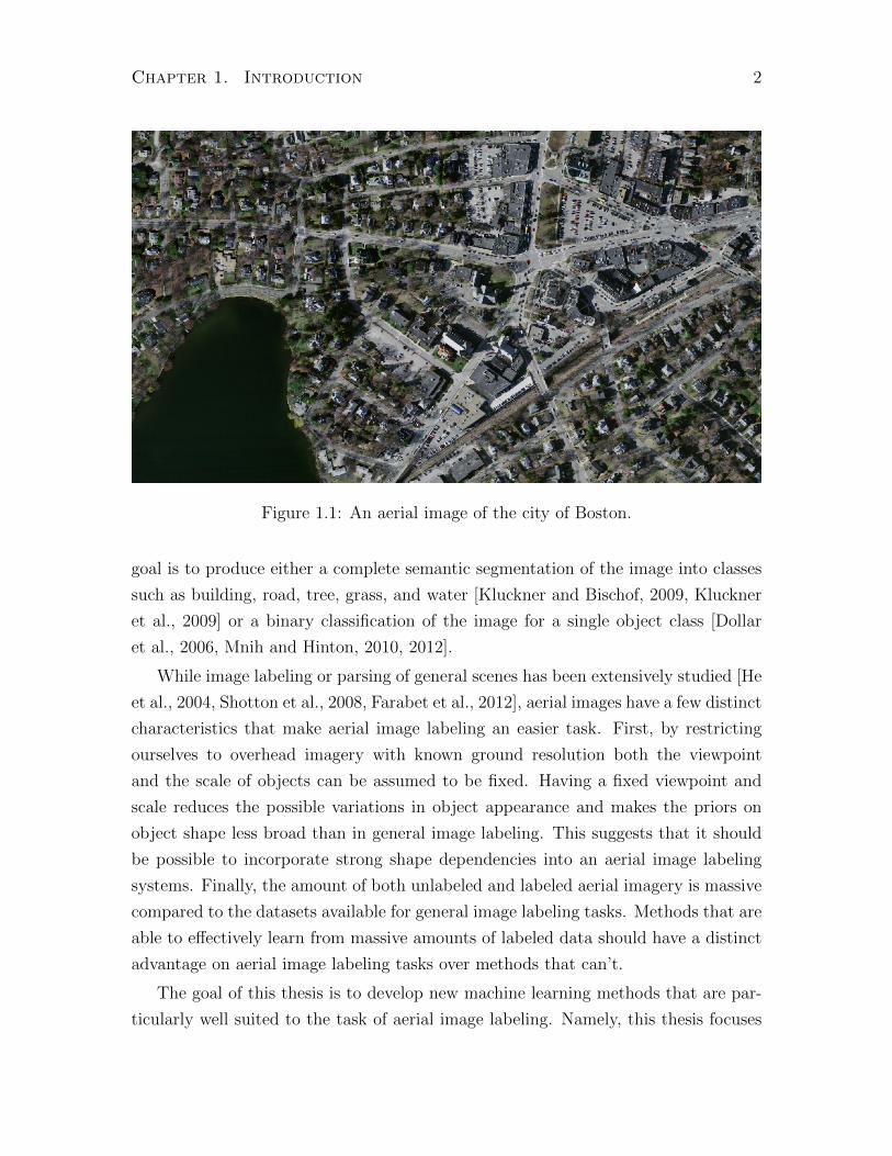
as a pixel labeling task. Given an aerial image like the one shown in Figure 1.1, the
1
Chapter 1. Introduction 2
Figure 1.1: An aerial image of the city of Boston.
goal is to produce either a complete semantic segmentation of the image into classes
such as building, road, tree, grass, and water [Kluckner and Bischof, 2009, Kluckner
et al., 2009] or a binary classification of the image for a single object class [Dollar
et al., 2006, Mnih and Hinton, 2010, 2012].
While image labeling or parsing of general scenes has been extensively studied [He
et al., 2004, Shotton et al., 2008, Farabet et al., 2012], aerial images have a few distinct
characteristics that make aerial image labeling an easier task. First, by restricting
ourselves to overhead imagery with known ground resolution both the viewpoint
and the scale of objects can be assumed to be fixed. Having a fixed viewpoint and
scale reduces the possible variations in object appearance and makes the priors on
object shape less broad than in general image labeling. This suggests that it should
be possible to incorporate strong shape dependencies into an aerial image labeling
systems. Finally, the amount of both unlabeled and labeled aerial imagery is massive
compared to the datasets available for general image labeling tasks. Methods that are
able to effectively learn from massive amounts of labeled data should have a distinct
advantage on aerial image labeling tasks over methods that can’t.
The goal of this thesis is to develop new machine learning methods that are par-
ticularly well suited to the task of aerial image labeling. Namely, this thesis focuses

Chapter 1. Introduction 3
on what we see as the three main issues in applying image labeling techniques to
aerial imagery:
• Context and Features: The use of context is important for successfully label-
ing aerial images because local colour cues are not sufficient for discriminating
between pairs of object classes like trees and grass, and roads and buildings.
Additionally, occlusions and shadows caused by trees and tall buildings often
make it impossible to classify a pixel without using any context information.
Since the number of input features grows quadratically with the width of an
input image patch, the number of parameters and the amount of computation
required for a naive approach also increases quadratically. For these reasons,
efficient ways of extracting discriminative features from a large image context
are necessary for aerial image labeling.
• Noisy Labels: When training a system to label images, the amount of labeled
training data tends to be a limiting factor. The most successful applications of
machine learning to aerial imagery have relied on existing maps. These provide
abundant labels, but the labels are often incomplete and sometimes poorly
registered, which hurts the performance of object detectors trained on them. In
order to successfully apply image labeling to buildings and other object types
for which the amount of label noise is high, new learning methods that are
robust to noise in the labels are required.
• Structured Outputs: Labels of nearby pixels in an image exhibit strong
correlations, and exploiting this structure can significantly improve labeling
accuracy. Due to the restricted viewpoint and fixed scale of aerial imagery,
the structure present in the labels is generally more rigid than that in general
image labeling, with shape playing an important role. In addition to being able
to handle shape constraints, a structured prediction method suited to aerial
imagery should also be able to deal with large datasets and noisy labels.
The main contribution of this thesis is a coherent framework for learning to label
aerial imagery. The proposed framework consists of a patch-based formulation of
aerial image labeling, new deep neural network architectures implemented on GPUs,
and new loss functions for training these architectures, resulting in a single model
that can be trained end-to-end while dealing with the issues of context, noisy labels,
and structured outputs.

Chapter 1. Introduction 4
Fully embracing the view of aerial image labeling as a large scale machine learning
task, we assemble a number of road and building detection datasets that far surpass
all previous work in terms of both size and difficulty. In addition to releasing the
first publicly available datasets for aerial image labeling we perform the first truly
large-scale evaluation of an aerial image labeling system on real-world data. When
trained on these road and building detection datasets our models surpass all published
models in terms of accuracy.
The rest of the thesis is organized as follows:
• Chapter 2 presents a brief overview of existing work on applying machine learn-
ing to aerial image data. Some related work on general image labeling that has
not been applied to aerial imagery is also covered.
• Chapter 3 presents our formulation of aerial image labeling as a patch-based
pixel labeling task as well as an evaluation of several different proposed architec-
tures. The main contribution is a GPU-based, deep convolutional architecture
that is capable of exploiting a large image context as well as learning discrim-
inative features. This chapter includes work previously published in Mnih and
Hinton [2010] and Mnih and Hinton [2012].
• Chapter 4 addresses the problem of learning from incomplete or poorly regis-
tered maps. The main contributions are loss functions that provide robustness
to both types of label noise and are suitable for training the architectures pro-
posed in Chapter 3. This work has been previously published in [Mnih and
Hinton, 2012].
• Chapter 5 explores ways of taking advantage of the structure present in the la-
bels. We investigate two complementary ways of performing structured predic-
tion – post-processing neural networks and Conditional Random Fields (CRFs).
We argue that neural networks are good at learning high-level structure while
CRFs are good at capturing low-level dependencies, with the combination of
the two approaches being particularly effective. We also show how to combine
a noise model from Chapter 4 with the proposed structured prediction models.
This chapter includes work previously published in Mnih et al. [2011] and Mnih
and Hinton [2012].

Chapter 1. Introduction 5
• Chapter 6 introduces the first large-scale publicly available datasets for road
and building detection which are both much larger and more challenging than
any datasets previously used in the literature. We evaluate our most promis-
ing models on the new datasets giving an indication of how well the proposed
algorithms work in the wild.
• Chapter 7 summarizes our most important findings and offers a discussion of
the most promising directions for improving our system.
Chapter 2
An Overview of Aerial Image
Labeling
This chapter aims to present a general overview of aerial image labeling methods. In
particular, we focus on approaches that make use of machine learning as opposed to
ad-hoc and knowledge-based approaches [Idelsohn, 1970, Bajcsy and Tavakoli, 1976,
Kettig and Landgrebe, 1976, Jr. et al., 1985] which account for much of the early
work on automating aerial image interpretation. While knowledge-based approaches
have led to some operational systems in limited domains, machine learning has led
to much of the recent progress in aerial image interpretation as well as progress on
related computer vision problems such as semantic image labeling [Shotton et al.,
2008].
We will use the term aerial imagery to refer to any type of two dimensional and
possibly multi-band data collected by an airborne sensor. In addition to imagery
taken by sensors that measure visible light, this includes sensors that measure other
kinds of electromagnetic radiation, such as infrared and hyperspectral sensors, as well
as sensors that do not measure electromagnetic radiation, such as airborne LIDAR,
which measures the distance to objects from the sensor.
6

Chapter 2. An Overview of Aerial Image Labeling 7
2.1 Early Work - Simple Classifiers and Local Fea-
tures
Some of the first applications of machine learning to aerial imagery considered the
task of classifying land cover, or terrain, into different classes, such as forest, water,
agricultural land, and built-up land. Early approaches tried to predict the discrete
class label ci at a pixel i from a vector xi of features at i [Decatur, 1989, Benediktsson
et al., 1990, Bischof et al., 1993, Paola and Schowengerdt, 1995], with the features
typically just taken to be the values at the different spectral bands at pixel i.
The Bayes’ classifier is one of simplest and most popular approaches to terrain
classification. The Bayes’ classifier makes explicit assumptions about the class condi-
tional distributions p(xi|ci = k) and the prior class probabilities P (ci = k) and uses
Bayes’ rule to obtain the posterior class probabilities P (ci = k|xi). Typically, the
class conditional distribution p(xi|ci = k) is assumed to have a multivariate normal
distribution with mean µk and covariance Σk. Various simplifying assumptions lead
to other popular classifiers. For example, assuming that Σk is diagonal leads to the
Naive Bayes classifier for continuous inputs while assuming that P (ci = k) = 1/K
leads to what is known in the remote sensing literature as the maximum likelihood
classifier [Paola and Schowengerdt, 1995].
The main drawback of the Bayes’ classifier is the need to explicitly specify the
class-conditional distribution p(xi|ci = k). Since the multivariate normal distribu-
tion is typically used for the class-conditional distributions, only linear or quadratic
decision boundaries can be learned by such a model. Neural networks became a pop-
ular alternative to the Bayes’ classifier because they directly model p(ci|xi = k) as a
differentiable function whose parameters are learned [Decatur, 1989, Lee et al., 1990,
Bischof et al., 1993]. This both sidesteps the need to specify p(xi|ci = k), and allows
for richer, non-linear decision boundaries to be learned when at least one hidden layer
of units with a non-linear activation function is used. Due to the ability to learn non-
linear decision boundaries neural networks tend to give higher classification accuracies
than various forms of the Bayes’ classifier [Decatur, 1989, Benediktsson et al., 1990].
Bischof et al. [Bischof et al., 1993] and Boggess [Boggess, 1993] explored adding
contextual information by using spectral values from a small patch centered at the
pixel of interest as the input to a neural network, allowing it to learn some contex-
tual features. However, such features were still very local since they used at most

Chapter 2. An Overview of Aerial Image Labeling 8
a 7 by 7 window for context. Others aimed to improve classification accuracy by
using hand-designed features that encode local textural information [Haralick et al.,
1973, Haralick, 1976, Lee et al., 1990]. Haralick et al. [Haralick, 1976] introduced
a popular set of features derived from gray level spatial dependence matrices Hd,θ,
where H(i, j)d,θ specifies the frequency at which gray level values i and j co-occur
at distance d and angle θ. Statistical quantities derived from Hd,θ were shown to be
good for discriminating between different types of textures. For example, the sum of
squares of the entries of Hd,θ can be used to discriminate coarse textures from fine
textures because the sum of squares should be higher for coarse textures than for fine
textures when d is small.
Since such systems were generally applied to low resolution imagery, with a single
pixel representing as much as 30x30 meters, local spectral cues were sufficient for
discriminating between broad classes of interest, such as forest and farmland, with
reasonably high accuracy. For example Bischof et al. [Bischof et al., 1993] report
accuracies in the range of 85% on a four class classification task using only the values
of seven spectral bands as input.
However, with increasing availability of higher resolution data, the focus shifted
to classifying aerial imagery into finer object classes, such as roads, cars, and trees.
At resolutions higher than one pixel per square meter, differences in object type,
shape and material as well as variations in weather and lighting conditions make it
impossible to accurately classify objects based on local cues alone.
2.2 Move to High-Resolution Data
The Ikonos and Quickbird satellites, launched in 1999 and 2001 respectively, began
acquiring panchromatic images of the surface of the Earth at resolutions of roughly
one square meter per pixel, significantly increasing the number of possible applications
of aerial image interpretation systems. Since at this resolution the classes of interest
are man-made objects such as buildings, roads, and cars, the approach of training
simple classifiers on very local spectral and textural features that was moderately
successful on low resolution images no longer leads to acceptable accuracy levels.
The approaches discussed in the previous section no longer work because they were
generally designed to do local texture classification, but the problem of classifying
high-resolution imagery is much more complex, requiring knowledge of shape and
Chapter 2. An Overview of Aerial Image Labeling 9
context in addition to texture.
During the move from low-resolution to high-resolution image labeling the most
notable trends were:
1. The switch to more powerful or sophisticated classifiers such as AdaBoost,
SVMs, and random forests.
2. The use of more spatial context and richer input features.
3. The use of much more data for training and testing.
4. The use of structured prediction methods such as Conditional Random Fields.
We will discuss the first three trends in some detail in the following subsections and
delay the discussion of structured prediction methods to a later, separate section.
2.2.1 Better classifiers
Discriminating between object classes with similar texture, such as roads and build-
ings, requires some knowledge of shape and context, which in turn leads to much
more complex decision boundaries than the ones required for discriminating between
wooded and built up areas in low-resolution imagery. Due to the need to learn such
highly nonlinear decision boundaries, applications of machine learning to high reso-
lution imagery have relied on more sophisticated classifiers such as SVMs, random
forests and various types of boosting.
While neural networks are able to learn nonlinear decision boundaries and have
been widely used in remote sensing applications, many researchers found them difficult
to train due to the presence of local optima [Benediktsson et al., 1990]. Support Vector
Machines presented an attractive alternative to neural networks because, like neural
networks, they are able to learn nonlinear decision boundaries, but, unlike neural
networks, SVMs optimize a convex loss function and do not suffer from the problem
of local optima. Since SVMs are essentially sophisticated template matchers and have
been shown to work poorly when applied as classifiers to raw image patches [LeCun
et al., 2004], they are generally used in combination with higher level features in
the computer vision community [Lazebnik et al., 2006]. Applications of SVMs to
aerial image interpretation have been much more primitive than in the computer
Chapter 2. An Overview of Aerial Image Labeling 10
vision community, with most papers using SVMs to classify pixels using only low-
level features [Huang et al., 2002, Song et al., 2005].
Some of the more successful approaches to labeling high resolution aerial imagery
have relied on various ensemble methods, with boosting and random forests being
particularly popular. Porway et al. [2008] developed a hierarchical model for aerial
image parsing that relied on bottom up detectors for cars, roads, parking lots and
buildings that were trained using different types of boosting. Other notable applica-
tions of boosting include the work of Dollar et al. [Dollar et al., 2006], who developed
a general framework for learning to detect image boundaries using a boosted pixel
classifier and presented some qualitative results on road detection, and the work of
Nguyen et al. [Nguyen et al., 2007] who used online boosting to learn a car detector.
A common reason for using boosting in these applications is its ability to perform
feature selection from a very large pool of features when the set of weak learners is
restricted to learners that look at a single feature. Dollar et al. [2006] were able to
use a pool of 50,000 filter responses as features for their edge classifier.
A random forest is another tree-based ensemble method that has been widely
used in image labeling applications. A random forest classifier consists of a number
of decision trees whose predictions are typically combined using majority voting. The
goal of the training procedure is to reduce the variance of the ensemble by trying to
produce decorrelated trees. This is achieved by learning each tree on a random subset
of the dataset and using a random subset of the input variables. A number of papers
by Kluckner et al. [Kluckner et al., 2009, Kluckner and Bischof, 2009] use random
forests for performing semantic classification of aerial images with impressive results.
While random forests and boosting of tree classifiers both construct ensembles of
trees, they do so in completely different ways, leading to clear advantages and dis-
advantages that may make one more suitable to aerial imagery applications. While
boosting has been found to perform better than random forests in several bake offs,
algorithms such as AdaBoost are known to perform poorly in the presence of outliers
or mislabeled training cases because they tend to emphasize the difficult cases during
training. This may be a serious limitation in the context of aerial image interpreta-
tion because perfectly registered and up-to-date label information is rarely available.
Random forests, on the other hand, are much less affected by mislabeled data because
each tree is built on a random subset of the training data using a random subset of
the input features and no special emphasis is placed on the difficult training cases.
Chapter 2. An Overview of Aerial Image Labeling 11
Additionally, random forests are embarrassingly parallelizable while boosting is much
more difficult to parallelize due to its sequential nature. Given these reasons random
forests seem to be somewhat better suited to aerial image classification.
2.2.2 Better features
The approach of using the values of multiple bands at a single pixel, or even a window
of a small size such as 5x5, as input to a classifier is hopeless on high resolution
imagery because the input simply does not contain enough information to discriminate
between object classes. The simplest way of addressing this problem is to use a larger
input window as input. Mnih and Hinton [Mnih and Hinton, 2010] showed that
increasing the size of the input patch from 24 by 24, which is already a large context
size compared to other work, to 64 by 64 significantly improves precision and recall
on a road detection task.
Simply using a large image patch for input can be slow even on modern computers
because the computational cost of applying a linear filter to a square patch scales
quadratically with the width of the patch. For this reason recent work has relied on
efficiently computable features in order to scale up to large context sizes [Kluckner
and Bischof, 2009, Nguyen et al., 2007, Dollar et al., 2006]. The most widely used class
of efficiently computable image features is the set of features that can be expressed
as a linear combination of sums of rectangular regions of the image [Viola and Jones,
2001]. To compute such filters efficiently, let I(x, y) be the value of the image intensity
of a single channel at location (x, y) and define
S(x, y) =∑x′≤x
∑y′≤y
I(x′, y′). (2.1)
S is known as the integral image of I and can be computed in time linear in the
number of pixels in the image. Once S is computed, the sum of any sub-rectangle of
I can be computed in constant time. For example, the sum of I over the rectangle
[a, b]× [c, d] can be computed as S(b, d)−S(b, c)−S(a, d)+S(a, c). Features that can
be computed efficiently using the integral image trick include special cases of Haar
wavelets [Viola and Jones, 2001] and histograms of oriented gradients.
Typically, people rely on filters from one or more popular filter banks for obtaining
input representations. Filters in the Haar basis, shown in Figure 3.10 (top), consist
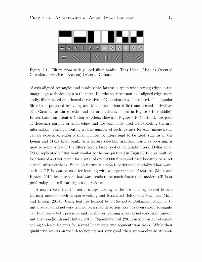
Chapter 2. An Overview of Aerial Image Labeling 12
Figure 2.1: Filters from widely used filter banks. Top) Haar. Middle) OrientedGaussian derivatives. Bottom) Oriented Gabors.
of axis aligned rectangles and produce the largest outputs when strong edges in the
image align with the edges in the filter. In order to detect non-axis aligned edges more
easily, filters based on oriented derivatives of Gaussians have been used. The popular
filter bank proposed by Leung and Malik uses oriented first and second derivatives
of a Gaussian at three scales and six orientations, shown in Figure 3.10 (middle).
Filters based on oriented Gabor wavelets, shown in Figure 3.10 (bottom), are good
at detecting parallel oriented edges and are commonly used for exploiting textural
information. Since computing a large number of such features for each image patch
can be expensive, either a small number of filters tend to be used, such as in the
Leung and Malik filter bank, or a feature selection approach, such as boosting, is
used to select a few of the filters from a large pool of candidate filters. Dollar et al.
[2006] replicated a filter bank similar to the one pictured in Figure 3.10 over multiple
locations of a 50x50 patch for a total of over 50000 filters and used boosting to select
a small subset of them. When no feature selection is performed, specialized hardware,
such as GPUs, can be used for learning with a large number of features [Mnih and
Hinton, 2010] because such hardware tends to be much faster than modern CPUs at
performing dense linear algebra operations.
A more recent trend in aerial image labeling is the use of unsupervised feature
learning methods such as sparse coding and Restricted Boltzmann Machines [Mnih
and Hinton, 2010]. Using features learned by a Restricted Boltzmann Machine to
initialize a neural network trained on a road detection task has been shown to signifi-
cantly improve both precision and recall over training a neural network from random
initialization [Mnih and Hinton, 2010]. Rigamonti et al. [2011] used a variant of sparse
coding to learn features for several linear structure segmentation tasks. While their
qualitative results on road detection are not very good, their system obtains state-of-

Chapter 2. An Overview of Aerial Image Labeling 13
the-art performance on a retinal blood vessel segmentation task. Such unsupervised
feature learning approaches tend to learn filters that resemble oriented edge detectors
and Gabor wavelets [Mnih and Hinton, 2010, Rigamonti et al., 2011] and have the
advantage of potentially being able to learn the best filters for the task at hand as
opposed to just selecting the best ones from a pool of features that appear at only a
few scales and orientations.
A different type of feature that has been shown to be immensely useful for aerial
image interpretation is height information. Kluckner et al. [Kluckner et al., 2009]
showed that using height in addition to rich appearance-only features boosts classifi-
cation accuracies by 10 to 20%. The result should not be surprising because height
information can help discriminate between very confusable pairs of objects such as
roads/buildings and grass/trees. Height information can either be derived directly
from LIDAR data or from overlapping image pairs using stereo techniques. While
extremely helpful, height information may be difficult to obtain because LIDAR data
is less widely available and more expensive than aerial imagery, and most aerial im-
agery comes in the form of non-overlapping orthorectified image tiles which do not
contain stereo information.
2.2.3 Larger datasets
In early work on aerial image labeling it was common to use a single image for both
training and testing [Bischof et al., 1993, Bruzzone and Prieto, 2000]. Such a small
amount of data cannot possibly cover a large range of variations in the appearance
of various objects leading to classifiers that are unlikely to work well on unseen data.
The limited size of the test set as well as its similarity to the training data means
that the accuracy levels reported in earlier work are unlikely to translate to larger
datasets. Recent applications of machine learning to high-resolution aerial imagery
have used much more training data. For example, Porway et al. [2008] used 120 images
ranging in size from 640x480 to 1000x1000 for training their hierarchical probabilistic
grammar model of aerial image annotations. Kluckner et al. [Kluckner et al., 2009,
Kluckner and Bischof, 2009] used three datasets of roughly 100 images with each
dataset covering between 5 and 8 square kilometers to train a random forest classifier,
while Mnih and Hinton [Mnih and Hinton, 2010] trained a large neural network on
130 large images that cover an area of roughly 500 square kilometers at a resolution of
Chapter 2. An Overview of Aerial Image Labeling 14
0.7 pixels per square meter. Datasets of this size are more likely to contain significant
variations in the appearance of objects and, when used for training, these datasets
make it much harder for powerful classifiers to overfit.
2.3 Structured Prediction
The labels of nearby image pixels tend to be highly dependent due to the spatial
coherence of images and incorporating such knowledge into a predictor should improve
its accuracy. This idea of exploiting structure in the output labels was used in some of
the earliest work on aerial image labeling [Kettig and Landgrebe, 1976] and continues
to be important. This section provides an overview of the three main approaches
to structured prediction, namely segmentation, post-classification, and probabilistic
approaches.
2.3.1 Segmentation
Segmentation-based approaches work by first segmenting an image and then classify-
ing entire regions instead of individual pixels. Such approaches were among the first
to be proposed and are still in use today, usually in combination with a probabilistic
approach. In early work, Kettig and Landgrebe [Kettig and Landgrebe, 1976] pro-
posed a procedure that first classified non-overlapping aerial image patches of size
4 by 4 into homogeneous and non-homogeneous regions. The non-homogeneous re-
gions were then classified pixel-by-pixel, while homogeneous regions were merged into
larger regions and then classified using a region classifier. The standard approach is
to oversegment the image into what are known as superpixels and then classify the
superpixels individually [He et al., 2006, Huang and Zhang, 2009]. A statistical ap-
proach such as a Conditional Random Field can then be used to exploit dependencies
in neighbouring superpixel labels, as was done by He at al. [He et al., 2006].
While initially used as a structured prediction method, more recently segmentation-
based methods have been used for reducing the complexity of image labeling prob-
lems [He et al., 2006]. Labeling a few hundred superpixels per image can be a lot
less computationally demanding than labeling thousands of pixels, allowing for more
complex models to be used. The main drawback of segmentation-based approaches
to structured prediction is that they are usually unable to recover from incorrect seg-

Chapter 2. An Overview of Aerial Image Labeling 15
mentations, which can be particularly problematic in the aerial image setting where
occlusion of objects by trees or buildings is common. Some extensions of this approach
can reduce such failures by generating multiple oversegmentations using different pa-
rameter settings and combining classifications of the different segmentations into a
single classification of the pixels [Kohli et al., 2009].
2.3.2 Post-classification
Post-classification approaches aim to let predictions at one pixel indirectly influence
predictions at nearby pixels. For example, salt and pepper noise can be reduced
without any learning by applying a majority vote filter to the outputs of a local
classifier. Alternatively, some classifier is used to obtain preliminary labels for all the
pixels and a second classifier is then trained to predict a new label for each pixel based
on the preliminary labels of nearby pixels. The hope is that this second classifier will
be able to clean up the output of the first classifier. Bischof et al. [Bischof et al.,
1993] trained a neural network that looks at a 5x5 window of predictions to predict a
new label for the middle pixel, improving classification accuracy by several percent.
Mnih and Hinton [Mnih and Hinton, 2010] used a neural network with a 64x64 input
window to clean up predictions of another neural network on a road detection task,
significantly improving both precision and recall.
2.3.3 Probabilistic Approaches
Probabilistic approaches directly model the conditional probability P (y|x) of the la-
bels y given the image x. By far the most widely used probabilistic model for struc-
tured prediction is the conditional random field, which models P (y|x) as a Markov
random field over the labels y that is globally-conditioned on the image x. More
precisely
P (y|x) = exp
(−∑c∈C
fc(yc,x)
)/Z(x), (2.2)
where C is a set of cliques over y, fc’s are potential functions, and Z(x) is the partition
function.
The most widely used form of CRFs in both aerial imaging applications and
the field of computer vision in general is the pairwise CRF, for which the model

Chapter 2. An Overview of Aerial Image Labeling 16
distribution takes the form
P (y|x) = exp
−∑i
U(yi,x)−∑i
∑j∈N(i)
Iij(yi, yj,x)
/Z(x), (2.3)
where i indexes the label sites and N(i) gives the neighbouring sites for site i. The
model has two types of potentials. Ui is the unary potential which determines how
well label yi agrees with the image x, while Iij is an interaction potential which
determines how well the labels at sites i and j agree with each other and, possibly,
the image x.
In image labeling applications of CRFs the graphical structure of the model is
almost always either a lattice or a tree. In a typical lattice the sites are laid out on
a grid with each site connected to either its 4 or 8 neighbours, depending on whether
the diagonal neighbours are connected. The lattice structure is generally used when
the pixels themselves or rectangular sets of pixels are used as the labeling sites. Such
CRFs have been applied to urban area detection [Zhong and Wang, 2007] and LIDAR
point classification [Niemeyer et al., 2008]. Tree structured CRFs are typically used
when the labeling sites are regions obtained by first segmenting the image. This
technique is often used for significantly reducing the number of random variables
over which the CRF is defined in order to speed up inference and learning [Modestino
and Zhang, 1989].
Pairwise CRFs are appealing for their simplicity, but since they use only pairwise
interaction potentials they seem to restrict one to only being able to encourage label
smoothness constraints. While smoothness is probably the most important constraint
for aerial image labeling applications, being able to include other types of constraints
is desirable. For example, the fact that roads tend to have different shape than
buildings is a very strong cue for distinguishing between roads and buildings. In
order to incorporate such knowledge into a model one would need to be able to
encode constraints on shape. Similarly, constraints based on layout could be useful
for detecting buildings because buildings tend to be next to roads. The multiscale
CRF model proposed by He et al. [2004] is an alternative to pairwise CRFs that
is able to learn the shape and layout of objects. For the case of binary labels y,
the CRF of He et al. [2004] is a conditional Restricted Boltzmann Machine with the
Chapter 2. An Overview of Aerial Image Labeling 17
model distribution given by
P (y|x) =∑h
exp(yTWh + hTbh + yT [bv + f(x)]
)/Z(x), (2.4)
where h is a vector of stochastic latent variables, f(x) is the vector of features ex-
tracted from the image x, and the model parameters are W,bh, and bv. Each latent
variable hj corresponds to a single feature of the labels y and can encode possible
shapes of objects as well as different arrangements of objects.
Probabilistic approaches to structured prediction are the most principled since
they can directly enforce smoothness and other constraints on the labels. The ability
to model complex distributions, however, often makes exact or efficient inference
intractable. In the case of CRFs, the models for which exact inference is tractable
tend to be simple models such as tree-structured CRFs, or lattice-structured CRFs
with sub-modular potentials. When working with more expressive classes of CRFs
one generally has to resort to approximate inference and learning procedures, making
the application of such models difficult.
2.3.4 Discussion of Structured Prediction
Out of the approaches to structured prediction we have discussed, methods based
on segmentation are the weakest because of their rigidity. Due to this weakness,
segmentation-based methods are now rarely used without being combined with a
probabilistic model. Nevertheless, segmentations of an image can provide useful
contextual information and have been used to construct new high-level image fea-
tures [Shotton et al., 2008] for use in CRFs. Post-classification approaches can work
well when a large training set is available [Mnih and Hinton, 2010], but such meth-
ods only incorporate indirect dependencies between the labels through the cleanup
process and are not as principled as probabilistic approaches. The combination of a
post-classification approach with a probabilistic model, such as a CRF, offers an inter-
esting possibility. Since incorporating rich dependencies among the labels y generally
leads to intractable inference, applying a CRF in which exact inference is tractable to
the outputs of a classifier would allow for incorporating complex dependencies over
the outputs without having to resort to inefficient or approximate inference.

Chapter 2. An Overview of Aerial Image Labeling 18
2.4 Source of Supervision
One important, yet rarely discussed, aspect of using machine learning for aerial im-
age interpretation is the source of the data. The vast majority of papers rely on
hand-labeled data for both training and testing [Bischof et al., 1993, Nguyen et al.,
2007, Porway et al., 2008, Kluckner et al., 2009, Kluckner and Bischof, 2009, Nguyen
et al., 2010] and since labeling images is a very time consuming process, the datasets
have been small in both aerial image applications and general image labeling work.
A typical aerial image dataset covers a relatively small area of a single city, ranging
anywhere between one square kilometer and ten square kilometers [Kluckner et al.,
2009, Kluckner and Bischof, 2009], which seriously limits the variability due to archi-
tectural styles, weather conditions, and seasonal variations. Good results obtained
by training and testing an image labeling approach on such a small amount of data
will not necessarily translate to good performance on an entire city, especially if the
city is different from the one seen during training. Hence, obtaining good sources
of accurately labeled data is important for both evaluating existing approaches and
training systems that are likely to work under varying conditions.
In some domains hand-labeling data in order to train a classifier is not necessary
because the label information is often readily available. For example, in the case
of road detection the locations of existing roads are typically known because they
are useful for navigation and not just as target labels in a machine learning task.
The abundance of accurately labeled data for road detection makes it a very good
candidate for evaluating existing aerial image interpretation systems as well as the
application of machine learning techniques. While recent work on road detection
has largely switched to using large, freely-available sources of data, such as Google
Maps [Dollar et al., 2006, Huang and Zhang, 2009, Rigamonti et al., 2011], these
papers still do not use very much data for training and testing.
For buildings, Google Maps can provide the locations of a substantial portion of
the buildings in almost any major city. This type of data can act as a source of noisy
labels, which are correct with very high probability when they indicate the presence
of an object and with lower, but still high, probability when they indicate the absence
of an object. Training a classifier on large amounts of this type of noisy data with a
robust loss function can potentially produce a much better detector than by using a
much smaller set of accurate labels. At present, there seem to be no applications of

Chapter 2. An Overview of Aerial Image Labeling 19
robust estimators to aerial image data with noisy labels.
For object classes such as cars or areas for which Google Maps possesses neither
accurate nor complete map information, hand-labeling data seems to be the only
option. While the use of crowdsourcing tools like Amazon Mechanical Turk can make
it easier to collect label information, the process can still be expensive and time
consuming to set up. When only a limited amount of labeled data is available it
is often possible to generate new labeled data by transforming existing data. In a
classification task, small translations or rotations can be applied to the input images,
but in order to apply the same idea to image labeling one must be able to realistically
transform both the image and the labels. On a road detection task, applying rotations
to each training case before it is processed has been shown to help prevent overfitting
and drastically improve performance on cities not seen during training [Mnih and
Hinton, 2010]. Applying affine photometric transformations to training images has
been shown to improve performance in a general image labeling task [Shotton et al.,
2008], and can be potentially even more useful for aerial imagery, where this process
could simulate things like varying levels of sunlight.

Chapter 3
Learning to Label Aerial Images
This chapter presents our patch-based framework for learning to label aerial images
and is divided into three parts. The first part describes the general framework, how
we use neural networks within the framework, as well as issues relating to generating
data and training and evaluating the models. In the second part of the chapter we
attempt to answer the question of what is a good neural network architecture for
aerial image labeling tasks by performing an extensive experimental comparison of
different architectures. In the last part, we present a qualitative evaluation of the
best neural network architecture on road and building detection tasks and attempt
to shed some light on what the neural networks are actually learning.
3.1 Patch-Based Labeling Framework
The input to our aerial image labeling system is a list of aerial images S = (S(1), . . . ,S(N))
and a list of corresponding map images M = (M(1), . . . , M
(N)). The aerial images
S(n) are assumed to be rectangular images with c channels and can be anything from
gray scale or RGB aerial images to elevation maps and hyperspectral images. For
each n, the map or label image M(n)
is an image of the same size as S(n) with M(n)
i
denoting the label for the ith pixel of S(n). For binary image labeling tasks, M(n)
will be either 1 or 0, typically representing the presence or absence of an object of
some class of interest. For multi-class problems, M(n)
will take on values from a set
of possible labels {1, . . . , L}. Figure 3.1 shows an example of an aerial image on the
left and the corresponding map image denoting the locations of roads on the right.
The goal of this thesis is to develop methods that use the training data S and M to
20

Chapter 3. Learning to Label Aerial Images 21
Figure 3.1: Sample aerial image (left) and a binary map (right) denoting the locationof roads.
learn to predict the label map for new unseen aerial images.
We propose a patch-based learning framework where the aim is to predict patches
of M(n)
from patches of S(n). Before precisely defining the learning setup, we simplify
notation by dropping the indices (n) from S(n) and M(n)
and instead refer to an aerial
image S and the corresponding map image M. Taking a probabilistic approach we
define the central problem of this thesis as one of learning a model of the distribution
P (n(M, i, wm)|n(S, i, ws)), (3.1)
where n(I, i, w) denotes the w × w patch of image I centered at pixel i. Hence, we
model the distribution of a wm×wm patch of labels conditioned on a larger, ws×wsaerial image patch centered at the same pixel. Typically wm should be smaller than
ws because some context is required for predicting the labels. While wm can be set
to 1 to predict one label at a time, it is generally more efficient to predict a small
patch of labels from the same context. This approach of predicting patches of labels
is in contrast to the approaches of Dollar et al. [2006], Kluckner et al. [2009], which
make separate predictions for each pixel.
To further simplify notation, we will use vectors s and m to denote an aerial
Chapter 3. Learning to Label Aerial Images 22
image patch n(S, i, ws) and the corresponding map patch n(M, i, wm) respectively.
For now we will ignore the dependencies among nearby labels and assume conditional
independence of the map labels given the aerial image patch s. Using this assumption
and the simplified notation, Equation 3.1 can be rewritten as
P (m|s) =
w2m∏
i=1
P (mi|s). (3.2)
We will refer to P (m|s) as the observed map distribution. While the probabilistic
formulation may seem unnecessary at first, its benefits will become apparent when
we consider the problem of dealing with noisy labels in Chapter 4.
We propose modeling the observed map distribution using neural networks. Neu-
ral networks are particularly well suited to aerial image labeling tasks because of
several distinct advantages. Most importantly, neural networks have been shown to
work particularly well on perceptual tasks with large amounts of labeled data, out-
performing expert-designed systems in multiple domains [Dahl et al., 2010, Sermanet
et al., 2012]. The large amounts of existing maps suggests that this success could
apply to tasks such as road and building detection, for which large labeled training
sets can be constructed. Another important benefit is the ease with which neural net-
works can be parallelized on modern GPUs, which will make it possible to efficiently
scale up our models to large input contexts and train them on large datasets.
We will use f to denote the functional form of our neural network model, which
maps an input aerial patch s to a distribution over the label patch m. f will always
have one input for each entry of s, but the number of outputs is determined by the
number of possible labels.
For binary labeling tasks, we use neural networks that have one output unit for
each pixel of the map patch m with the output of unit i representing the predicted
probability that the ith label is 1. Since they encode probabilities, these output units
use the logistic activation function defined as σ(x) = 1/(1+exp(−x)). More formally,
fi(s) = σ(ai(s)) = P (mi = 1|s)
where fi is the value of the ith output unit and ai is the total input to the ith output
unit.
For multi-class labeling tasks, we use neural networks f with one softmax output

Chapter 3. Learning to Label Aerial Images 23
unit for each map patch pixel. The ith softmax unit outputs a vector with L compo-
nents which encodes distribution over the possible labels for pixel i. If we let ail be
the total input to component l of softmax unit i, and fil be the predicted probability
that map pixel i has label j, then
fil(s) = exp(ail(s))/Z = P (mi = l|s),
where Z =∑
l exp(ail)(s).
In order to simplify the presentation for the remainder of the thesis we will only
consider binary aerial image labeling tasks. Most of the techniques we will present
can be trivially extended to the multi-class setting by replacing sigmoid outputs with
softmax outputs, but we will provide the necessary details whenever the extension of
a technique to the multi-class setting is not obvious.
3.1.1 Learning
We learn the parameters of the neural networks by minimizing the negative log like-
lihood of the training data under our model. For binary data, the negative log
likelihood under the model in Equation 3.2 takes the form of a cross entropy between
the map patch m and the predicted label probabilities fi(s)
L(S,M) =∑
allpatches
w2m∑
i=1
(mi ln fi(s) + (1− mi) ln(1− fi(s))) . (3.3)
The outer sum of the objective L is over all possible patches in the training data.
Since there is a very large number of patches in our dataset we use stochastic gradient
descent with minibatches for optimizing L. For datasets that fit in memory, we
generate minibatches by repeatedly selecting a random pair (S(n), M(n)
) and sampling
a random patch from (S(n), M(n)
). For datasets that don’t fit in memory, we keep
a buffer of N ′ pairs of image/label images in memory and generate minibatches by
sampling patches at random from this buffer. By periodically replacing one of the N ′
pairs in the buffer with one of the N − N ′ pairs outside the buffer we approximate
random sampling of patches from the entire dataset.

Chapter 3. Learning to Label Aerial Images 24
Preprocessing
We have not explored the issue of preprocessing with the exception of relatively simple
contrast normalization. We normalize each input patch by subtracting the average
value computed over the patch and dividing by the standard deviation computed
over the entire dataset. Using more sophisticated types of preprocessing, such a local
contrast normalization is likely to lead to additional improvements in performance.
Adding Rotations
We found that it is useful to rotate each pair of image and label patches by a random
angle during learning. Since many cities have large areas where the road network
forms a grid, training on data without rotations will result in a model that is better at
detecting roads and buildings at certain orientations. Figure 3.3 shows three patches
taken from the Toronto Roads dataset with a clear bias in the orientations of the
roads. By randomly rotating the training cases the resulting models do not favour
objects in any particular orientation. The improvement is particularly noticeable on
infrequently appearing objects like highways, for which the orientation bias can be
even stronger than for normal roads.
Tuning Hyperparameters
When training neural nets with stochastic gradient descent one generally has to set a
number of hyper parameters including the learning rate, the amount of momentum,
the type and amount of weight decay, the mini batch size, and possibly others. We
did not separately tune these parameters for each architecture because doing so would
require a massive amount of computation. We chose the values of hyperparameters
shared by all models by selecting the values that maximize the performance of a shal-
low fully-connected network on the validation set of the Toronto Roads dataset. In
the few cases where we tried tuning the values of these hyperparameters for individ-
ual models or architectures we saw slight improvements in precision and recall, but
the order of models in terms of performance remained the same as for fixed hyperpa-
rameters. For this reason we believe that using the same values for hyperparameters
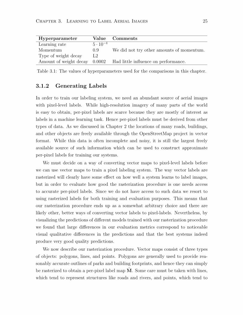
shared by all models is a reasonable thing to do when comparing models. Table 3.1
shows the hyperparameter values used for the comparisons in this chapter.
Chapter 3. Learning to Label Aerial Images 25
Hyperparameter Value CommentsLearning rate 5 · 10−4
Momentum 0.9 We did not try other amounts of momentum.Type of weight decay L2Amount of weight decay 0.0002 Had little influence on performance.
Table 3.1: The values of hyperparameters used for the comparisons in this chapter.
3.1.2 Generating Labels
In order to train our labeling system, we need an abundant source of aerial images
with pixel-level labels. While high-resolution imagery of many parts of the world
is easy to obtain, per-pixel labels are scarce because they are mostly of interest as
labels in a machine learning task. Hence per-pixel labels must be derived from other
types of data. As we discussed in Chapter 2 the locations of many roads, buildings,
and other objects are freely available through the OpenStreetMap project in vector
format. While this data is often incomplete and noisy, it is still the largest freely
available source of such information which can be used to construct approximate
per-pixel labels for training our systems.
We must decide on a way of converting vector maps to pixel-level labels before
we can use vector maps to train a pixel labeling system. The way vector labels are
rasterized will clearly have some effect on how well a system learns to label images,
but in order to evaluate how good the rasterization procedure is one needs access
to accurate per-pixel labels. Since we do not have access to such data we resort to
using rasterized labels for both training and evaluation purposes. This means that
our rasterization procedure ends up as a somewhat arbitrary choice and there are
likely other, better ways of converting vector labels to pixel-labels. Nevertheless, by
visualizing the predictions of different models trained with our rasterization procedure
we found that large differences in our evaluation metrics correspond to noticeable
visual qualitative differences in the predictions and that the best systems indeed
produce very good quality predictions.
We now describe our rasterization procedure. Vector maps consist of three types
of objects: polygons, lines, and points. Polygons are generally used to provide rea-
sonably accurate outlines of parks and building footprints, and hence they can simply
be rasterized to obtain a per-pixel label map M. Some care must be taken with lines,
which tend to represent structures like roads and rivers, and points, which tend to
Chapter 3. Learning to Label Aerial Images 26
represent small objects like houses and trees, because the vector representations do
not provide per-pixel information. We attempt to generate reasonable soft per-pixel
labels by applying simple smoothing to the rasterized objects. We define the label
map M for linear or point features as
Mi = e−d(i)2
σ2 , (3.4)
where d(i) is the Euclidean distance, in pixels, between location i and the nearest
object in the map. The smoothing parameter σ depends on the scale of the aerial
images being used as well as the type of object being rasterized. For example σ should
probably be higher for roads than for trees. This soft weighting scheme accounts for
some uncertainty in the location and shape of objects represented by lines and points.
3.1.3 Evaluating Predictions
The most common metrics for evaluating road detection systems are precision and
recall, which are known as correctness and completeness in the remote sensing litera-
ture [Wiedemann et al., 1998]. The precision is the fraction of predicted road pixels
that are true roads , while the recall of a set of predictions is the fraction of true road
pixels that were correctly detected.
Since the the vector maps we use to generate pixel labels are only accurate up
to a few pixels we compute relaxed precision and recall scores instead of exact ones.
Namely, in our experiments recall represents the fraction of true road pixels that
are within ρ pixels of a predicted road pixel, while precision represents the fraction
of predicted road pixels that are within ρ pixels of a true road pixel. Relaxing the
completeness and correctness measures in this manner is common practice when eval-
uating road detection systems [Wiedemann et al., 1998]. The slack parameter ρ was
set to 3 pixels for all experiments performed in this thesis.
Since the methods presented in this thesis predict the probability of each label
belonging to the class of interest, it is possible to trade off precision for recall by
varying the threshold for making a concrete prediction. One common way of evalu-
ating probabilistic binary classifiers is using precision-recall curves, which show the
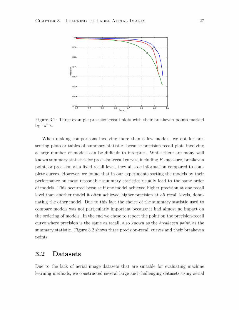
trade-off between precision and recall for all threshold values. We use precision-recall
curves for presenting quantitative comparisons involving a small number of models
because presenting entire curves conveys the most information.
Chapter 3. Learning to Label Aerial Images 27
0.3 0.4 0.5 0.6 0.7 0.8 0.9 1.0Recall
0.3
0.4
0.5
0.6
0.7
0.8
0.9
1.0
Prec
isio
n
Figure 3.2: Three example precision-recall plots with their breakeven points markedby ”x”’s.
When making comparisons involving more than a few models, we opt for pre-
senting plots or tables of summary statistics because precision-recall plots involving
a large number of models can be difficult to interpret. While there are many well
known summary statistics for precision-recall curves, including F1-measure, breakeven
point, or precision at a fixed recall level, they all lose information compared to com-
plete curves. However, we found that in our experiments sorting the models by their
performance on most reasonable summary statistics usually lead to the same order
of models. This occurred because if one model achieved higher precision at one recall
level than another model it often achieved higher precision at all recall levels, domi-
nating the other model. Due to this fact the choice of the summary statistic used to
compare models was not particularly important because it had almost no impact on
the ordering of models. In the end we chose to report the point on the precision-recall
curve where precision is the same as recall, also known as the breakeven point, as the
summary statistic. Figure 3.2 shows three precision-recall curves and their breakeven
points.
3.2 Datasets
Due to the lack of aerial image datasets that are suitable for evaluating machine
learning methods, we constructed several large and challenging datasets using aerial

Chapter 3. Learning to Label Aerial Images 28
images of the Greater Toronto Area. We used these datasets for all experiments
performed in Chapters 3, 4, and 5. Unfortunately, the imagery used to construct these
datasets is not publicly available because we were not aware of several repositories
of free high-resolution aerial imagery at the time. Chapter 6 will present the first
large-scale publicly available datasets for road and building detection along with
benchmarks of the most promising models developed in this thesis. We now describe
the characteristics of the proprietary datasets used in the next three chapters.
Toronto Roads Dataset
The Toronto Roads dataset consists of roughly 500 square kilometers of training data,
48 square kilometers of test data, and 8 kilometers of validation data at a resolution
of 1.2m per pixel. This dataset contains both urban and suburban areas of Toronto.
The target road map for the Toronto Roads dataset contains some omitted roads but
has only minor registration problems.
Hamilton Roads Dataset
The Hamilton Roads dataset consists of a training set of roughly 250 square kilometers
of the city of Hamilton at a resolution of 1.2m per pixel. The target road map for
this dataset contains frequent registration errors in addition to some omitted roads
and for this reason we only used it to study the effectiveness of the robust losses
introduced in Chapter 4. Figure 4.7(a) shows a representative subset of the Hamilton
Roads dataset.
GTA Buildings Dataset
The GTA Building dataset consists of roughly 600 square kilometers of imagery of
the Greater Toronto Area. The target map contains significant omission errors and
includes mostly large buildings, with most but not all houses unlabeled. Due to the
presence of noise in the targets, we used only 8 square kilometers of hand-labeled
data for validation.

Chapter 3. Learning to Label Aerial Images 29
Figure 3.3: Three sample input patches from the Toronto Roads dataset. The redsquare denotes the region for which labels are predicted.
3.3 Architecture Evaluation
We now proceed to an evaluation of different neural network architectures on the task
of road detection. We train the neural networks to predict 16× 16 map patches from
64 × 64 input aerial image patches in the Toronto Roads dataset. Figure 3.3 shows
three example input patches, with a red square denoting the region for which label
predictions are to be made. In the Toronto Roads dataset each pixel corresponds to
1.44 square meters, making a 64× 64 input patch contain sufficient information for a
human to correctly identify the objects in the target region.
We evaluate a number of architecture design choices, including the number of
layers, the connectivity pattern between layers, types of hidden units, and the use of
pooling. While several such studies have been conducted for the problem of object
recognition [Jarrett et al., 2009, Coates et al., 2011] it is unclear whether the same
conclusions apply for image labeling tasks. For example, max-pooling discards in-
formation about the location of features and while this may be beneficial for object
recognition it may not lead to similar improvements for image labeling, where the
precise location of objects needs to be predicted. Moreover, due to the small size of
most object recognition datasets design choices that help reduce overfitting seem to
provide substantial benefits, but as we will see later in this chapter overfitting is far
less of a problem for our datasets so it is unclear whether methods that aim to reduce
overfitting will offer any benefits at all.
3.3.1 One Layer Architectures
We first compare different neural networks with a single hidden layer. All the net-
works we compare have 3 ·642 inputs that correspond to a contrast-normalized 64×64

Chapter 3. Learning to Label Aerial Images 30
RGB aerial image patch. The input is fed to a hidden layer that extracts roughly
12000 features and applies a nonlinearity, possibly followed by pooling. The number
of hidden units is held approximately the same in order to fix the size of the extracted
feature representation to be roughly the same. In all of the networks the hidden layer
is followed by a fully connected output layer of 256 logistic output units. We compare
the following one-layer architecture types differing only in the connectivity pattern of
the hidden layer:
Fully connected architecture: As the name suggests, this architecture has a fully
connected hidden layer. Since a fully connected network with 12000 hidden units has
roughly 150 million parameters it is slow to train even on a GPU. We instead use a
fully connected network with 4096 hidden units and roughly 50 million parameters,
making it somewhat more manageable.
Factored architecture: The hidden layer of a factored architecture approximates
a full m × n weight matrix as a dot product of two low rank matrices UTV where
U is an f ×m matrix and V is an f × n matrix. This low rank approximation can
greatly reduce the number of free parameters over the full weight matrix. We use a
factored hidden layer with 2048 factors f and 12000 hidden units. This architecture
has roughly the same number of parameters as the fully connected one but has three
times more hidden units.
Local untied architecture: The hidden layer of a locally connected architecture
drastically reduces the number of parameters over both fully connected and factored
architectures by only connecting each hidden unit to a small subpatch of the in-
put. To precisely define the connectivity pattern, assume that the input units of
a locally connected layer make up a win × win image consisting of multiple chan-
nels. The input image is divided into evenly spaced filter sites by moving a wf × wfwindow over the image by a stride of wstr vertically and horizontally, for a total of
((win − wf )/wstr + 1)2 filter sites. A different set of f filters of size wf × wf and
consisting of the same number of channels as the input image is applied at each filter
site. Hence, a single locally connected layer results in f · ((win − wf )/wstr + 1)2 hid-
den units and f · ((win − wf )/wstr + 1)2 ·w2f · c parameters, where c is the number of
input channels.
Chapter 3. Learning to Label Aerial Images 31
Layer typeUnit type
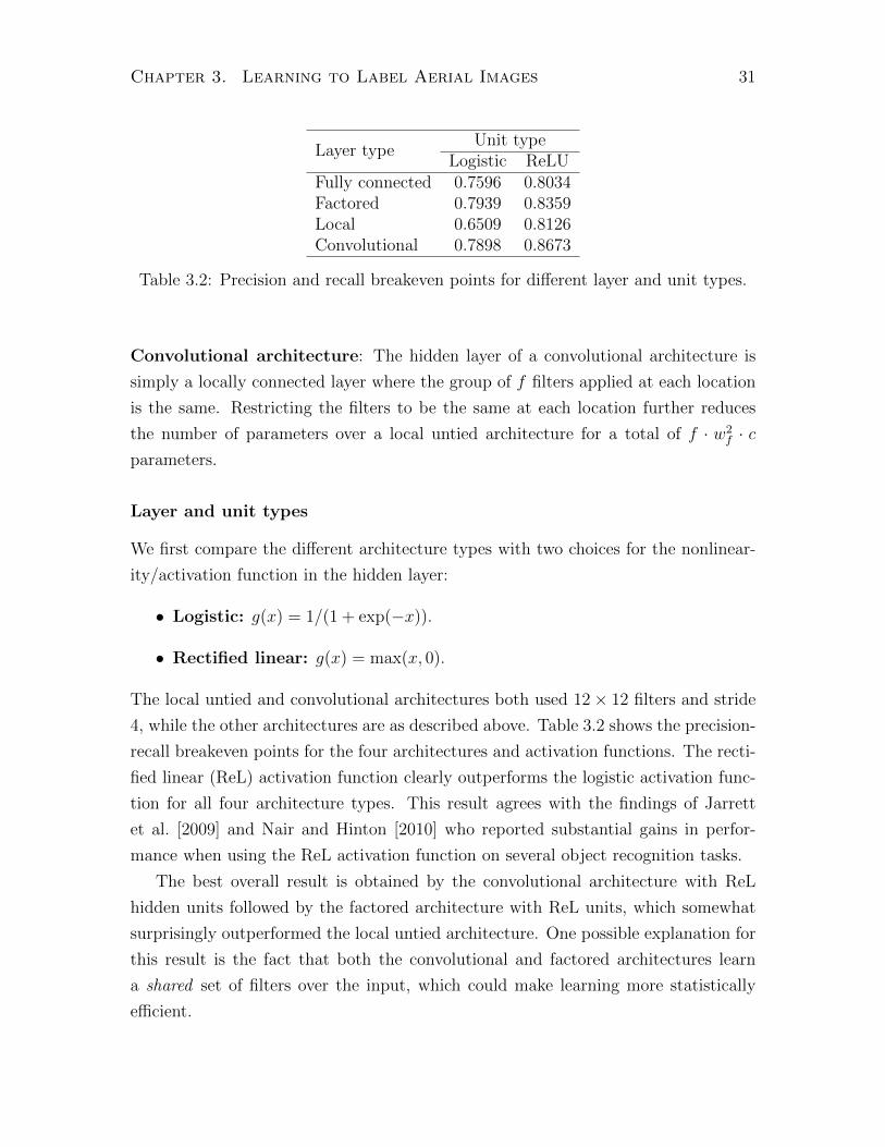
Logistic ReLUFully connected 0.7596 0.8034Factored 0.7939 0.8359Local 0.6509 0.8126Convolutional 0.7898 0.8673
Table 3.2: Precision and recall breakeven points for different layer and unit types.
Convolutional architecture: The hidden layer of a convolutional architecture is
simply a locally connected layer where the group of f filters applied at each location
is the same. Restricting the filters to be the same at each location further reduces
the number of parameters over a local untied architecture for a total of f · w2f · c
parameters.
Layer and unit types
We first compare the different architecture types with two choices for the nonlinear-
ity/activation function in the hidden layer:
• Logistic: g(x) = 1/(1 + exp(−x)).
• Rectified linear: g(x) = max(x, 0).
The local untied and convolutional architectures both used 12× 12 filters and stride
4, while the other architectures are as described above. Table 3.2 shows the precision-
recall breakeven points for the four architectures and activation functions. The recti-
fied linear (ReL) activation function clearly outperforms the logistic activation func-
tion for all four architecture types. This result agrees with the findings of Jarrett
et al. [2009] and Nair and Hinton [2010] who reported substantial gains in perfor-
mance when using the ReL activation function on several object recognition tasks.
The best overall result is obtained by the convolutional architecture with ReL
hidden units followed by the factored architecture with ReL units, which somewhat
surprisingly outperformed the local untied architecture. One possible explanation for
this result is the fact that both the convolutional and factored architectures learn
a shared set of filters over the input, which could make learning more statistically
efficient.
Chapter 3. Learning to Label Aerial Images 32
No pooling 2x2 pooling 3x3 pooling 4x4 pooling0.81
0.82
0.83
0.84
0.85
0.86
0.87
0.88
Bre
ake
ven p
oin
t on p
reci
sion/r
eca
ll cu
rve
Local untiedConvolutional
(a)
8 12 16 20Filter width in pixels
0.80
0.81
0.82
0.83
0.84
0.85
0.86
0.87
Bre
ake
ven p
oin
t on p
reci
sion/r
eca
ll cu
rve
Local untiedConvolutional
(b)
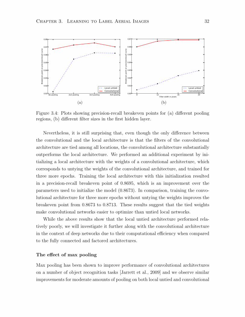
Figure 3.4: Plots showing precision-recall breakeven points for (a) different poolingregions, (b) different filter sizes in the first hidden layer.
Nevertheless, it is still surprising that, even though the only difference between
the convolutional and the local architecture is that the filters of the convolutional
architecture are tied among all locations, the convolutional architecture substantially
outperforms the local architecture. We performed an additional experiment by ini-
tializing a local architecture with the weights of a convolutional architecture, which
corresponds to untying the weights of the convolutional architecture, and trained for
three more epochs. Training the local architecture with this initialization resulted
in a precision-recall breakeven point of 0.8695, which is an improvement over the
parameters used to initialize the model (0.8673). In comparison, training the convo-
lutional architecture for three more epochs without untying the weights improves the
breakeven point from 0.8673 to 0.8713. These results suggest that the tied weights
make convolutional networks easier to optimize than untied local networks.
While the above results show that the local untied architecture performed rela-
tively poorly, we will investigate it further along with the convolutional architecture
in the context of deep networks due to their computational efficiency when compared
to the fully connected and factored architectures.
The effect of max pooling
Max pooling has been shown to improve performance of convolutional architectures
on a number of object recognition tasks [Jarrett et al., 2009] and we observe similar
improvements for moderate amounts of pooling on both local untied and convolutional

Chapter 3. Learning to Label Aerial Images 33
architectures on image labeling tasks. We evaluated the effects of max pooling when
placed on top of the hidden layers of local untied and convolutional architectures with
64 filters of size 12 and stride 4. We compared pooling over overlapping regions of
size 2 × 2, 3 × 3, and 4 × 4 with stride 1 The results shown in Figure 3.4(a) show
that max pooling helps both untied local and convolutional architectures, with the
best results obtained with 3 × 3 pooling regions. The fact that pooling over larger
regions leads to smaller improvements is not surprising given that the network needs
to maintain precise locations of certain features.
The effects of filter sizes and strides
We now look at the effect of filter size on the performance of local network archi-
tectures. Figure 3.4(b) shows the precision-recall breakeven points for networks with
filters of size 8, 12, 16, and 20 and filter stride 4. Both convolutional and untied
local networks seem to benefit from larger filter sizes, with larger improvements seen
for untied local networks. This positive dependence on filter size is the opposite of
what Coates et al. [2011] observed for unsupervised feature learning on object detec-
tion tasks. It is unclear whether the difference is due to our use of supervised feature
learning, differing filter strides, or simply the type of data we use. Since Coates et al.
[2011] used a stride of 1 for the filter size experiments we investigated the possibility
that smaller filters are better at smaller strides and found that this is not the case.
3.3.2 Two Layer Architectures
We now turn to a similar analysis of two layer architectures of untied local and con-
volutional layers with ReL hidden units. The first layer of both types of architectures
had 64 filters of size 12× 12 with stride 4. We investigated the effect of varying the
sizes of the filters and pooling regions in the second hidden layer.
The effect of max pooling
We fixed the second layer of both architectures to have 128 4× 4 filters with stride 1
and then compared using no pooling, 2×2 max pooling, and 3×3 max pooling on top
of the second layer. Figure 3.5(a) shows a plot of precision-recall breakeven points for
the different model configurations. Convolutional architectures do not seem to benefit
from pooling in the second layer. Given that the first layer uses 3 max pooling, it is

Chapter 3. Learning to Label Aerial Images 34
No pooling 2x2 pooling 3x3 pooling0.875
0.880
0.885
0.890
0.895
0.900
0.905
0.910
0.915B
reake
ven p
oin
t on p
reci
sion/r
eca
ll cu
rve
Local untiedConvolutional
(a)
3 4 5 6Filter width in pixels
0.87
0.88
0.89
0.90
0.91
0.92
Bre
ake
ven p
oin
t on p
reci
sion/r
eca
ll cu
rve
Local untiedConvolutional
(b)
Figure 3.5: Plots showing precision-recall breakeven points for (a) different poolingregions, (b) different filter sizes in the second hidden layer.
likely that using any additional pooling in the second layer loses too much information
about the precise location of object parts to help on a pixel labeling task. Given this
result, it is somewhat surprising that untied local architectures seem to benefit from
max pooling in the second layer. As in the single hidden layer case, this effect is likely
explained by the fact that adding pooling to an untied local architecture encourages
filters in the same feature pool to be similar, with the resulting performance boost
outweighing the decrease in performance due to the lower spatial resolution.
The effects of filter sizes and strides
We compared using filters of size 3, 4, 5, and 6 with stride 1 in the second layer of both
architecture types. Figure 3.5(b) shows the precision-recall points for the different
model configurations. As in the single hidden layer case, larger filters seem to work
better in both types of architectures, with a more noticeable improvement for untied
local architectures. We also performed a control experiment to see whether using a
smaller stride while holding the number of hidden units fixed improved results and
found that, as in the one layer case, there was no significant change.
Discussion
The local untied and convolutional architectures improve on the breakeven point for
a shallow factored model by more than 0.04 and 0.08 respectively while using far

Chapter 3. Learning to Label Aerial Images 35
0.70 0.75 0.80 0.85 0.90 0.95 1.000.70
0.75
0.80
0.85
0.90
0.95
1.00
Two layerThree layers, fully connectedThree layers, factoredThree layers, convolutional
(a)
0.70 0.75 0.80 0.85 0.90 0.95 1.000.70
0.75
0.80
0.85
0.90
0.95
1.00
Three layersFour layers, fully connectedFour layers, factoredFive layers, fully connected
(b)
Figure 3.6: A comparison of precision-recall curves for deep architectures. (a) Acomparison of different choices for the third layer of a deep architecture. (b). Acomparison of three, four and five layer networks.
fewer parameters. These results also show that increasing network depth clearly im-
proves the accuracy of untied and convolutional architectures on aerial image labeling
tasks. Overall, convolutional architectures perform noticeably better than untied ar-
chitectures suggesting that the ability to learn different filters at different locations
is either not helpful or is far outweighed by the benefits of weight sharing found in
convolutional nets.
3.3.3 Deeper Architectures
Given the substantial improvements in precision and recall that we gained by adding
a second layer to locally connected architectures we investigate whether adding even
more layers helps. We start with a two layer convolutional network which has 64
12× 12 filters and stride 4 in the first layer and 112 4× 4 filters with stride 1 in the
second layer and add layers until it stops producing better results.
We compare three different choices for the third hidden layer: a fully connected
layer with 4096 hidden units, a factored layer with 2048 factors and 4096 hidden units,
and a convolutional layer with 80 3× 3 filters and stride 1 for a total of 3920 hidden
units. The precision-recall plots for the three models as well as the base two layer
model are shown in Figure 3.6(a). There is a noticeable improvement in precision
and recall from adding a third layer. The fully connected layer leads to the largest
improvement, but at the cost of using more parameters and computation.
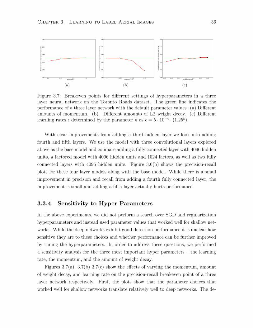
Chapter 3. Learning to Label Aerial Images 36
0.8 0.85 0.9 0.95Momentum
0.90
0.91
0.92
0.93
0.94
0.95Br
eake
ven
poin
t on
prec
isio
n/re
call
curv
e
(a)
0 0.0002 0.002 0.02L2 Weight Cost
0.90
0.91
0.92
0.93
0.94
0.95
Brea
keve
n po
int o
n pr
ecis
ion/
reca
ll cu
rve
(b)
k=-3 k=-2 k=-1 k=0 k=1 k=2 k=3log learning rate
0.90
0.91
0.92
0.93
0.94
0.95
Brea
keve
n po
int o
n pr
ecis
ion/
reca
ll cu
rve
(c)
Figure 3.7: Breakeven points for different settings of hyperparameters in a threelayer neural network on the Toronto Roads dataset. The green line indicates theperformance of a three layer network with the default parameter values. (a) Differentamounts of momentum. (b). Different amounts of L2 weight decay. (c) Differentlearning rates ε determined by the parameter k as ε = 5 · 10−4 · (1.25k).
With clear improvements from adding a third hidden layer we look into adding
fourth and fifth layers. We use the model with three convolutional layers explored
above as the base model and compare adding a fully connected layer with 4096 hidden
units, a factored model with 4096 hidden units and 1024 factors, as well as two fully
connected layers with 4096 hidden units. Figure 3.6(b) shows the precision-recall
plots for these four layer models along with the base model. While there is a small
improvement in precision and recall from adding a fourth fully connected layer, the
improvement is small and adding a fifth layer actually hurts performance.
3.3.4 Sensitivity to Hyper Parameters
In the above experiments, we did not perform a search over SGD and regularization
hyperparameters and instead used parameter values that worked well for shallow net-
works. While the deep networks exhibit good detection performance it is unclear how
sensitive they are to these choices and whether performance can be further improved
by tuning the hyperparameters. In order to address these questions, we performed
a sensitivity analysis for the three most important hyper parameters – the learning
rate, the momentum, and the amount of weight decay.
Figures 3.7(a), 3.7(b) 3.7(c) show the effects of varying the momentum, amount
of weight decay, and learning rate on the precision-recall breakeven point of a three
layer network respectively. First, the plots show that the parameter choices that
worked well for shallow networks translate relatively well to deep networks. The de-
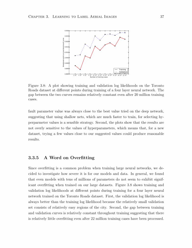
Chapter 3. Learning to Label Aerial Images 37
2 ·106 4 ·106 6 ·106 8 ·106 10 ·106 12 ·106 14 ·106 16 ·106 18 ·106 20 ·106 22 ·106
Number of training cases
0.890
0.895
0.900
0.905
0.910
0.915
0.920
0.925
0.930
Bre
ake
ven p
oin
t on p
reci
sion/r
eca
ll cu
rve
TrainingValidation
Figure 3.8: A plot showing training and validation log likelihoods on the TorontoRoads dataset at different points during training of a four layer neural network. Thegap between the two curves remains relatively constant even after 20 million trainingcases.
fault parameter value was always close to the best value tried on the deep network,
suggesting that using shallow nets, which are much faster to train, for selecting hy-
perparmeter values is a sensible strategy. Second, the plots show that the results are
not overly sensitive to the values of hyperparameters, which means that, for a new
dataset, trying a few values close to our suggested values could produce reasonable
results.
3.3.5 A Word on Overfitting
Since overfitting is a common problem when training large neural networks, we de-
cided to investigate how severe it is for our models and data. In general, we found
that even models with tens of millions of parameters do not seem to exhibit signif-
icant overfitting when trained on our large datasets. Figure 3.8 shows training and
validation log likelihoods at different points during training for a four layer neural
network trained on the Toronto Roads dataset. First, the validation log likelihood is
always better than the training log likelihood because the relatively small validation
set consists of relatively easy regions of the city. Second, the gap between training
and validation curves is relatively constant throughout training suggesting that there
is relatively little overfitting even after 22 million training cases have been processed.
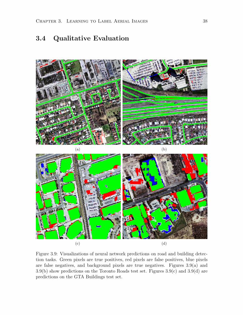
Chapter 3. Learning to Label Aerial Images 38
3.4 Qualitative Evaluation
(a) (b)
(c) (d)
Figure 3.9: Visualizations of neural network predictions on road and building detec-tion tasks. Green pixels are true positives, red pixels are false positives, blue pixelsare false negatives, and background pixels are true negatives. Figures 3.9(a) and3.9(b) show predictions on the Toronto Roads test set. Figures 3.9(c) and 3.9(d) arepredictions on the GTA Buildings test set.

Chapter 3. Learning to Label Aerial Images 39
We now apply the lessons learned in the previous section to training a large neural
network on road and building detection datasets. The network we train has four
hidden layers. The first layer is convolutional with 64 filters of size 12 and stride
4, and is followed by size 3 stride 1 max pooling layer. The second hidden layer is
convolutional with 112 filters of size 4 and stride 1 followed by another convolutional
layer with 112 filters of size 3 and stride 1. The last hidden layer is fully connected and
has 4096 hidden units. All four hidden layers use rectified linear units. We trained
two copies of this network on the Toronto Roads and GTA Buildings datasets. The
network trained on the Toronto Roads dataset achieved a breakeven point of 0.928
on the test set, while the network trained on the GTA Buildings dataset achieved a
breakeven point of 0.818 on its test data.
To get some idea of what the numbers mean we visualize the predictions of both
networks at their breakeven points. Figure 4.7 visualizes the predictions on parts
of the test set by colour coding each pixels based on whether it was a true or false
positive/negative, providing many interesting insights into how the networks work.
The predictions on the Toronto Roads dataset, shown in Figures 3.9(a) and 3.9(b),
demonstrate that the network is very good at detecting multiple types of roads includ-
ing two-lane roads in residential areas, multi-lane roads, and even highways. While
the false positives and false negatives show several failure cases for our model, they
also illustrate several problems with the data. For example, the network sometimes
makes predictions for disconnected blobs of road in paved areas, which end up being
counted as false positives. This is an artifact of the network making independent pre-
dictions for each pixel, making it difficult for the network to realize that it is creating
a disconnected component. Such errors can be avoided by incorporating structure
into the predictions and Chapter 5 examines different ways of doing so. Another
common type of mistake is a false negative caused by the shadow of a tall building.
While we do not do so in this thesis, some form of local contrast normalization will
likely help in such cases.
We also see that the network is often penalized for making a road prediction in a
paved area. These predictions show up as false positives because narrow alleys and
roads leading into malls or industrial areas are often not included in vector maps.
Whenever this type of mislabeling occurs in the training data the neural network is
penalized for what is essentially a correct prediction.
The predictions for the network trained on the GTA Buildings dataset are shown
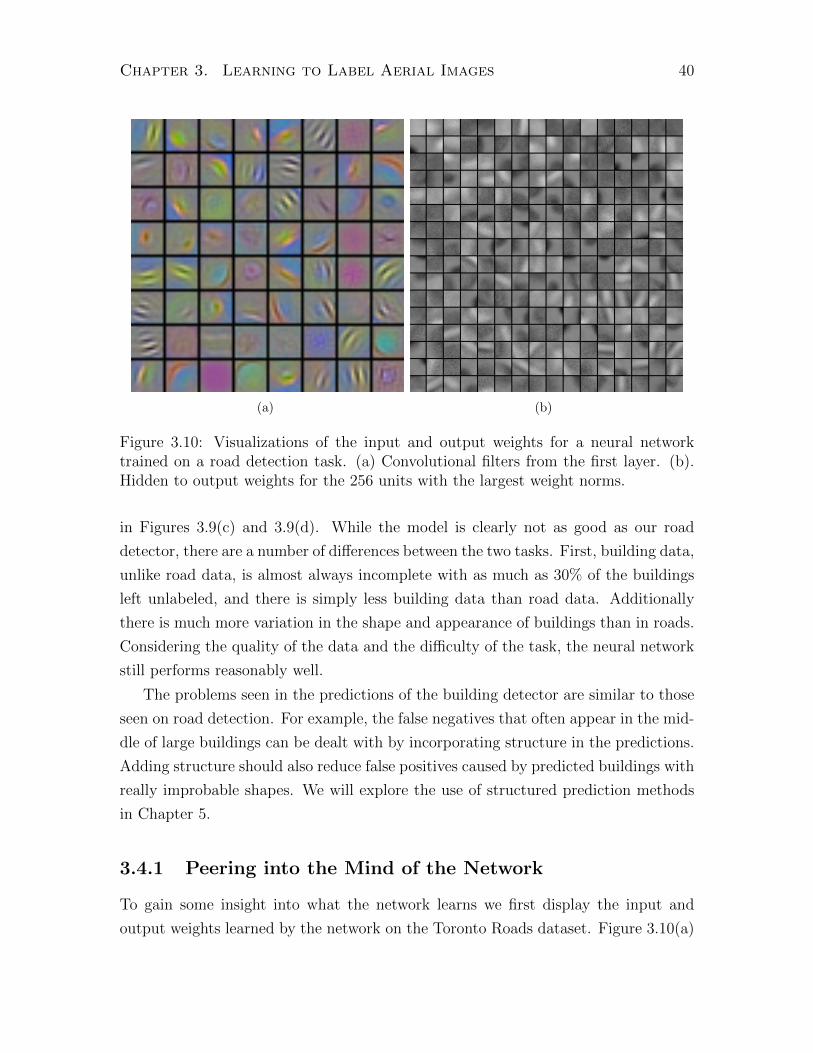
Chapter 3. Learning to Label Aerial Images 40
(a) (b)
Figure 3.10: Visualizations of the input and output weights for a neural networktrained on a road detection task. (a) Convolutional filters from the first layer. (b).Hidden to output weights for the 256 units with the largest weight norms.
in Figures 3.9(c) and 3.9(d). While the model is clearly not as good as our road
detector, there are a number of differences between the two tasks. First, building data,
unlike road data, is almost always incomplete with as much as 30% of the buildings
left unlabeled, and there is simply less building data than road data. Additionally
there is much more variation in the shape and appearance of buildings than in roads.
Considering the quality of the data and the difficulty of the task, the neural network
still performs reasonably well.
The problems seen in the predictions of the building detector are similar to those
seen on road detection. For example, the false negatives that often appear in the mid-
dle of large buildings can be dealt with by incorporating structure in the predictions.
Adding structure should also reduce false positives caused by predicted buildings with
really improbable shapes. We will explore the use of structured prediction methods
in Chapter 5.
3.4.1 Peering into the Mind of the Network
To gain some insight into what the network learns we first display the input and
output weights learned by the network on the Toronto Roads dataset. Figure 3.10(a)

Chapter 3. Learning to Label Aerial Images 41
Figure 3.11: Visualization of the derivatives of the loss function with respect to theinput pixel values.
shows all 64 convolutional filters from the first layer and 256 of the output filters with
the highest L2 norm. Not surprisingly, the convolutional filters the network learns are
oriented edge and grating detectors, often with an overlaid lower frequency opposing
yellow/blue and green/red patterns. Convolutional neural networks tend to learn
similar filters on other object detection tasks [Krizhevsky, 2011]. The output filters
learned by the network, shown in Figure 3.10(b), also exhibit interesting structure
that falls into several groups. Two of the most prominent groups are entire road
segments at different orientations and filters that make a neutral prediction for much
of the patch and a strong vote for the absence of a road in one of the corners.
Another informative way of visualizing the neural network is through a sensitivity
analysis, which involves looking at the gradient of the loss function with respect to
the inputs at different data points. Figure 3.11 shows a number of input aerial image
patches from the Toronto Roads dataset with the squared gradient with respect to
the input for each data point overlaid in red. Hence, a change to the values of the
input pixels highlighted in red will cause a big change to the value of the loss function.
We see that whenever a piece of road is present in the centre 16× 16 patch for which
the neural net is making predictions there is a strong gradient on the road pixels.
3.5 Conclusions and Discussion
We have shown that our patch-based framework for learning to label aerial imagery
with deep neural networks can achieve good performance on challenging real world
road and building detection datasets. The results show that there is a clear advantage
to using deep networks over shallow ones and that convolutional networks outperform
networks with other types of connectivity. We also saw that while there is a bene-
Chapter 3. Learning to Label Aerial Images 42
fit from using a small amount of max pooling, using too much max pooling hurts
performance on pixel labeling tasks.
While the framework addresses the basic problem of efficiently learning discrim-
inative features from large amounts of labeled aerial imagery, it has a number of
shortcomings. Most importantly, the neural network architectures we examined in
this chapter make separate predictions for each pixel. As we saw in the previous
section, this leads to a number of undesirable artifacts in the predictions, including
disconnected blobs of road and gaps in roads and buildings. Chapter 5 will address
the problem of how to efficiently incorporate rich structure into the predictions while
maintaining the ability to learn from very large datasets.
Another problem with the framework is the underlying assumption that the train-
ing data is perfectly labeled. Figure 4.7 clearly shows problems with the labels which
likely hurt the neural networks during training. This issue has not been studied widely
in machine learning or computer vision and Chapter 4 will attempt to modify our
learning procedure in ways that reduce the effects of noise typically found in maps
on the neural networks.
In addition to addressing the above limitations there are many other ways to
improve the performance of our system that we do not address in this thesis. One
interesting possibility is the use of losses other than negative log likelihood defined
on individual label pixels. For example, Turaga et al. [2009] showed how directly
optimizing a measure of image segmentation leads to much better segmentations
than by optimizing individual pixel disagreement. In our case, optimizing the area
under the precision-recall curve could lead to similar improvements because it is a
better measure of the quality of the detections than log likelihood.
Another way of improving our system is by performing a more extensive hyperpa-
rameter search. While we have only looked at using a fixed learning rate and weight
cost for all layers, using different values for each layer could both speed up learning
and improve the overall performance. Since doing so requires searching over a very
large space of parameters, doing so by brute force search would require a tremendous
amount of computation. A more efficient way of performing this search is using the re-
cently developed methods for doing Bayesian global optimization of hyper parameter
values [Bergstra et al., 2011, Snoek et al., 2012].

Chapter 4
Learning to Label from Noisy Data
The preceding chapter demonstrated that it is possible to use readily available aerial
imagery along with vector metadata from sources such as OpenStreetMap to obtain
state-of-the-art performance on aerial image labeling tasks. While OpenStreetMap
provides an abundance of label information that is clearly of high-enough quality to
learn from, the label information is often incomplete or noisy. In particular we classify
the most common data inaccuracies into two types of noise:
• Omission noise occurs when an object that appears in an aerial image does
not appear in the map. This is the case for many buildings (even in major cities)
due to incompleteness of the maps. It is also true for small roads and alleys,
which tend to be omitted from maps, often with no clear criterion for when they
should be omitted. An example of omission noise is shown in Figure 4.1(a).
• Registration noise occurs when the location of an object in a map is inaccu-
rate. Such errors are quite common because not requiring pixel level accuracy
makes maps cheaper to produce for human experts without significantly re-
ducing their usefulness for most purposes. An example of registration noise is
shown in Figure 4.1(b).
The presence of these kinds of errors in the training labels can significantly reduce
the accuracy of classifiers trained on such data.
This chapter shows how one can deal with the presence of both kinds of noise in the
training labels. We present two robust loss functions that can be incorporated into our
image labeling framework. The first loss function reduces the effect of omission errors,
43

Chapter 4. Learning to Label from Noisy Data 44
(a) (b)
Figure 4.1: Road locations derived from a map are shown in red. (a) Example ofomission noise. (b) Example of registration noise.
while the second loss function reduces the effects of both omission and translation
errors. We then demonstrate the effectiveness of these loss functions on road and
building detection tasks.
4.1 Dealing With Omission Noise
Omission noise, as shown in Figure 4.1(a), occurs when some map pixels are labeled
as not belonging to the object class of interest when they, in fact, do. When trained
on data containing a substantial number of such pixels a classifier will be penalized
for correctly predicting the value of 1 for pixels affected by omission noise. This will
cause a classifier to be less confident and potentially increase the false negative rate.
We propose using a robust loss function that explicitly models asymmetric omis-
sion noise in order to reduce its effect on the final classifier. We recall that in Chapter 3
the observed map distribution p(m|s) was modeled directly by a neural network. By
doing maximum-likelihood learning under this model we are implicitly assuming that
the training data consists of true samples from a model in this class of models. In
order to account for the possibility of noisy data we take the approach of explicitly
modeling the noise process. We assume a generative process where the true, uncor-
rupted, and unobserved map patch m is first generated from the aerial image patch
s according to some distribution p(m|s). The corrupted, observed map m is then
generated from the uncorrupted m according to a noise distribution p(m|m).
For now, we assume that conditioned on m, all components of m are independent

Chapter 4. Learning to Label from Noisy Data 45
and that each mi is conditionally independent of all mj for j 6= i. The observed map
distribution that corresponds to this model can then be obtained by marginalizing
out m from p(m|m)p(m|s), leading to
p(m|s) =∑m
p(m|m)p(m|s) (4.1)
=
w2m∏
i=1
∑mi
p(mi|mi)p(mi|s). (4.2)
The noise distribution p(mi|mi) is assumed to be the same for all pixels i, and is
parameterized by the parameters
θ0 = p(mi = 1|mi = 0) and,
θ1 = p(mi = 0|mi = 1).
In the presence of omission noise, we expect that θ0 � θ1 because the probability
that the observed label mi is 1 given that the true label mi is 0 should be very close
to 0, while the probability that the observed mi is 0 given that the true label mi is 1
should still be small but not as close to 0 as θ0.
There are several different ways of determining the values of the parameters θ0
and θ1 – they can be learned along with the neural network weights, selected using a
validation set, or set by hand. We found that learning the parameters along with the
other weights is difficult. This is likely due to the possibility of small changes to θ0 and
θ1 resulting in large changes to the derivatives with respect to the other parameters
because θ0 and θ1 are parameters of the loss. While this issue could potentially
be resolved with second order optimization methods, we did not investigate this
possibility and set the values of the parameters using a validation set.
We refer to this model as the asymmetric Bernoulli noise model, or the ABN model
for short. While in the noise-free setting of Chapter 3 the observed map distribution
was modelled directly by a neural network, in the noisy setting, we instead use the
neural network to model the true map distribution p(m|s). Learning can still be done
efficiently by minimizing the negative log probability of the training data under the
ABN model given in Equation 4.2. Since the ABN model factorizes over the pixels i
and there is only a single Bernoulli latent variable mi for each pixel i, the derivative
of the negative log probability can be found directly.

Chapter 4. Learning to Label from Noisy Data 46
0.0 0.2 0.4 0.6 0.8 1.0mi
−1.0
−0.8
−0.6
−0.4
−0.2
0.0
∂lnp(m
i|s)/∂xi
Noise free modelABN model
Figure 4.2: The plot shows the derivative of the log probability with respect to theinput to the ith output unit for varying predictions mi. In this example, the observedlabel mi is set to 0 while the parameters of the ABN model are θ0 = 0.001 andθ1 = 0.05. The noise free model penalizes incorrect predictions more than the ABNmodel, especially when the prediction is incorrect and confident.
In order to gain some insight into how the noise model affects learning, we contrast
the derivatives of the negative log probability of the data with and without a noise
model. Let xi and mi be the input and output to the ith unit of the neural network
respectively. In the noise-free scenario, the derivative of − log p(m|s) with respect to
xi is mi − mi. Hence, in the absence of a noise model, the learning procedure tries
to make the prediction mi closer to the observed label mi. Under the ABN model,
the derivative of the negative log probability of the data takes the form p(mi =
1|mi, s) − mi. Hence, the learning procedure tries to make the prediction mi close
to the posterior probability that the unobserved true label mi is 1. This has the
effect that the neural network gets penalized less for making a confident but incorrect
prediction. Figure 4.2 demonstrates how the derivatives of the log probability of the
data differ for the noise-free and the ABN models differ as a function of the prediction
mi.
4.2 Dealing With Registration Noise
Registration noise occurs when an aerial image and the corresponding map are not
perfectly aligned. As shown in Figure 4.1(b), the error in alignment between the
map and the aerial image can vary spatially over the dataset and hence cannot be

Chapter 4. Learning to Label from Noisy Data 47
corrected by a single global translation. In order to deal with a large class of possible
misalignments we make the simplifying assumption that the registration error between
the image and the map is approximately constant in any wm′ × wm′ region. This
assumption is likely to hold true whenever the error in registration varies over the
dataset sufficiently slowly.
4.2.1 Translational Noise Model
We extend the robust loss function we introduced in the previous section for dealing
with omission noise to also handle local registration errors. As with the ABN model,
we introduce a generative model of the observed map patches. On a high level, the
generative model works by first generating an uncorrupted and perfectly registered
map from the aerial image, then selecting a random subpatch of the true map, and
generating the observed map by corrupting the selected subpatch with asymmetric
noise. More formally, the generative process is as follows:
1) An uncorrupted and perfectly registered true map patch m of size wm′ × wm′is generated from s according to p(m|s). Typically wm′ is at least wm + 2tmax where
tmax is the maximum possible registration error/translation between the map and
aerial image measured in pixels. We allow for the possibility that wm′ is greater
than wm + 2tmax because it may be useful to make the size of the region for which
misalignments are assumed to be approximately constant be different from the size
of the predicted patch.
2) A translation variable t is sampled from some distribution p(t) over T + 1
possible translations 0, . . . , T . In this thesis, we use T = 8, where t = 0 corresponds
to no translation while the other eight values index the eight possible translations by
tmax pixels in the vertical and horizontal directions as well as their combinations (see
Figure 4.3).
3) An observed map is sampled from the translational noise distribution
p(m|m, t) = p(m|Crop(m, t)) (4.3)
=
w2m∏
i=1
pABN(mi|Crop(m, t)i), (4.4)
where Crop(m, t) selects a wm by wm subpatch from the wm′ by wm′ patch m ac-
cording to the translation variable t as shown in Figure 4.3, and pABN(mi|mi) is the

Chapter 4. Learning to Label from Noisy Data 48
t=1 t=2t=2 t=3
t=4 t=0 t=5
t=6 t=7 t=8
Figure 4.3: Demonstration of the Crop(m, t) function. For each dark gray patchrepresenting m, the lighter gray subpatch highlights the area cropped by Crop(m, t)for each value of the translation parameter t.
pixelwise asymmetric binary noise model defined in the previous section.
We attempt to parameterize this noise model using as few parameters as possible.
By assuming that all non-zero translations are equiprobable, we are able to param-
eterize the prior over translations using a single parameter θt = P (t = 0). For all
other translations, t > 0 we get that P (t = i) = (1 − P (t = 0))/T = (1 − θt)/T .
This assumption is reasonable because we only consider 1 and 2 pixels as the values
of tmax, but it would not hold for larger values of tmax where the diagonal transla-
tions should be less probable than the vertical and horizontal ones. Hence, we use a
total of four parameters for the entire model: tmax, θt, and two parameters needed
to parameterize pABN(mi|mi). We refer to this generative model as the translational
asymmetric binary noise model, or the TABN model for short.
4.2.2 Learning
The observed map distribution under the TABN model is given by
p(m|s) =T∑t=0
p(t)∑m
p(m|m, t)p(m|s), (4.5)
where the true map distribution p(m|s) is modeled by a neural network. In contrast to
the ABN model, where the map distribution factors over pixels, the map distribution
of the TABN model does not factor, making learning less straightforward. We simplify
the learning process by setting the parameters of p(t) and p(m|m, t) using a validation
Chapter 4. Learning to Label from Noisy Data 49
set and only learning the parameters of the neural network modeling p(m|s). We learn
parameters by minimizing the negative log likelihood under the model in Equation 4.5
using the EM-algorithm with a partial, approximate M-step. We demonstrate how
the required EM updates can be performed efficiently.
M-step: The the expected complete data log-likelihood for the TABN model is
given by
Q(θ) =∑t
∑m
p(m, t|m, s) ln p(t)p(m|m, s)p(m|s, θ). (4.6)
While the goal of the M-step is to maximize Q(θ) with respect to θ, this is not possible
for our model because Q(θ) is a nonlinear function due to p(m|s, θ) being modelled
by a neural network. We instead perform a partial approximate M-step by doing one
minibatch update of stochastic gradient descent on the objective Q(θ).
We recall that p(m|s, θ) =∏
i p(mi|s, θ) and that p(mi = 1|s, θ) = σ(xi), where
xi is the input to the ith output unit of the neural network and σ(x) is the logistic
sigmoid function. We compute the derivatives of Q(θ) with respect to the xi’s because
the derivative of Q(θ) with respect to any other parameter can be easily computed
using backpropagation from the quantities we compute.
We begin by rewriting the expected complete log likelihood as
Q(θ) =∑t
∑m
p(m, t|m, s) ln p(m|s)
=∑i
∑m
p(m|m, s) ln p(mi|s)
where we rewrote log p(m|s, θ) as a summation over the marginals of p(m|s) and
summed out the translation variable t. We also dropped the terms involving p(t) and
p(m|m, s) because their parameters are held fixed. It is possible to further simplify
Q(θ) by summing out mj for all j 6= i in each term of the outer summation to get
Q(θ) =∑i
∑mi
p(mi|m, s) ln p(mi|s)
= p(mi = 1|m, s) ln p(mi = 1|s) + (1− p(mi = 1|m, s)) ln(1− p(mi = 1|s))
= p(mi = 1|m, s) lnσ(xi) + (1− p(mi = 1|m, s)) ln(1− σ(xi).
Chapter 4. Learning to Label from Noisy Data 50
Finally, by recognizing the last term as a binary cross entropy we immediately obtain
∂
∂xiQ(θ) = p(mi = 1|m, s)− mi, (4.7)
where mi = σ(x) is the output of the ith unit of the neural network. This error
derivative for the update performed by the M-step has the intuitive form of the
difference between the predicted probability of the label for the pixel being 1 and the
posterior probability of the true label for that pixel being 1 under the model.
E-step: The role of the E-step is to compute p(mi|m, s) for use in the M-step,
and as we will show, this computation can be done in time T · w2m by exploiting the
structure of the noise model.
We begin by expressing the posterior marginals p(mi|m, s) as
p(mi|m, s) =
∑t
∑m−i
p(t)p(m|m, t)p(m|s)
/p(m|s)
=
∑t
p(t)∏j 6=i
∑mj
p(mj|mj, t)p(mj|s)
/p(m|s).
Now let Ct be the set of indices of pixels of m that are cropped for transformation t.
Since this set has w2m entries we slightly abuse notation and also use it to index into
m using the one-to-one pixel correspondence. We use Ct to define the intermediate
quantity
Pt =∏i∈Ct
(∑mi
p(mi|mi)p(mi|s)
), (4.8)
and notice that we can conveniently rewrite the above expression for p(mi|m, s) in
terms of Pt by performing two substitutions. First, we rewrite the observed map dis-
tribution p(m|s) in the denominator as∑
t p(t) ·Pt. The second substitution involves
replacing the product over pixels j in the summation in the numerator by Pt with
the term for pixel i replaced by p(mi|mi)p(mi|s). Putting everything together leads
to the final expression
p(mi|m, s) =
[∑t
p(t) · Pt ·p(mi|mi)p(mi|s)∑mip(mi|mi)p(mi|s)
]/
[∑t
p(t) · Pt]. (4.9)

Chapter 4. Learning to Label from Noisy Data 51
This way of computing the posterior marginals is rather efficient because it involves
only T different per-pixel computations.
The learning procedure is slightly complicated by allowing wm′ , the width of the
region for which registration error is assumed to be constant, to substantially differ
from wm, the width of region predicted by the neural network. While we always set
wm to 16, we found that setting wm′ to 18 or 20 to allow 1 or 2 pixel translation
of a 16 × 16 patch resulted in a model that is too flexible. It was simply too easy
for the model to cheat by always choosing to translate its patch of predictions to
incur a smaller loss. This effect is greatly reduced by setting wm′ to a value several
times larger than wm because it makes it much harder to explain a poor prediction
by translating it. We found that using wm′ = 4wp + 2tmax leads to a model with the
right amount of flexibility for our high resolution data.
To apply the noise model with this value of wm′ , we construct the wm′×wm′ patch
m out of 16 non-overlapping wp × wp patches predicted by the neural net. We then
find the wm′ ×wm′ patch of posterior marginals p(mi|m, s) as described above, break
it up into 16 non-overlapping wp×wp subpatches, and backpropagate the derivatives
from all the subpatches through the neural network.
4.2.3 Understanding the Noise Model
In order to demonstrate how the translational noise model works in practice, we used
the TABN model to train a neural network to detect roads from poorly registered
road data and plot the target labels, the model predictions, and the inferred true
labels for several test cases. Figure 4.4 shows target map labels in the top row, model
predictions in the middle row, and means of the marginals of the true map posterior
p(m|m, s) in the bottom row. These examples show how the TABN model is able to
correctly realign the target map with the aerial images.
4.3 Results
4.3.1 Omission Noise
We begin by evaluating the effectiveness of the ABN noise model on the Toronto
Roads and GTA Buildings datasets. We estimate that the omission rate is less than
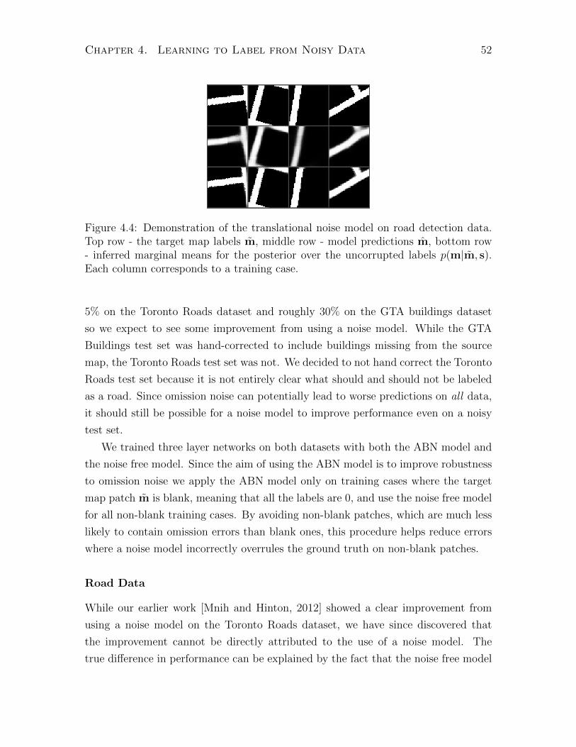
Chapter 4. Learning to Label from Noisy Data 52
Figure 4.4: Demonstration of the translational noise model on road detection data.Top row - the target map labels m, middle row - model predictions m, bottom row- inferred marginal means for the posterior over the uncorrupted labels p(m|m, s).Each column corresponds to a training case.
5% on the Toronto Roads dataset and roughly 30% on the GTA buildings dataset
so we expect to see some improvement from using a noise model. While the GTA
Buildings test set was hand-corrected to include buildings missing from the source
map, the Toronto Roads test set was not. We decided to not hand correct the Toronto
Roads test set because it is not entirely clear what should and should not be labeled
as a road. Since omission noise can potentially lead to worse predictions on all data,
it should still be possible for a noise model to improve performance even on a noisy
test set.
We trained three layer networks on both datasets with both the ABN model and
the noise free model. Since the aim of using the ABN model is to improve robustness
to omission noise we apply the ABN model only on training cases where the target
map patch m is blank, meaning that all the labels are 0, and use the noise free model
for all non-blank training cases. By avoiding non-blank patches, which are much less
likely to contain omission errors than blank ones, this procedure helps reduce errors
where a noise model incorrectly overrules the ground truth on non-blank patches.
Road Data
While our earlier work [Mnih and Hinton, 2012] showed a clear improvement from
using a noise model on the Toronto Roads dataset, we have since discovered that
the improvement cannot be directly attributed to the use of a noise model. The
true difference in performance can be explained by the fact that the noise free model
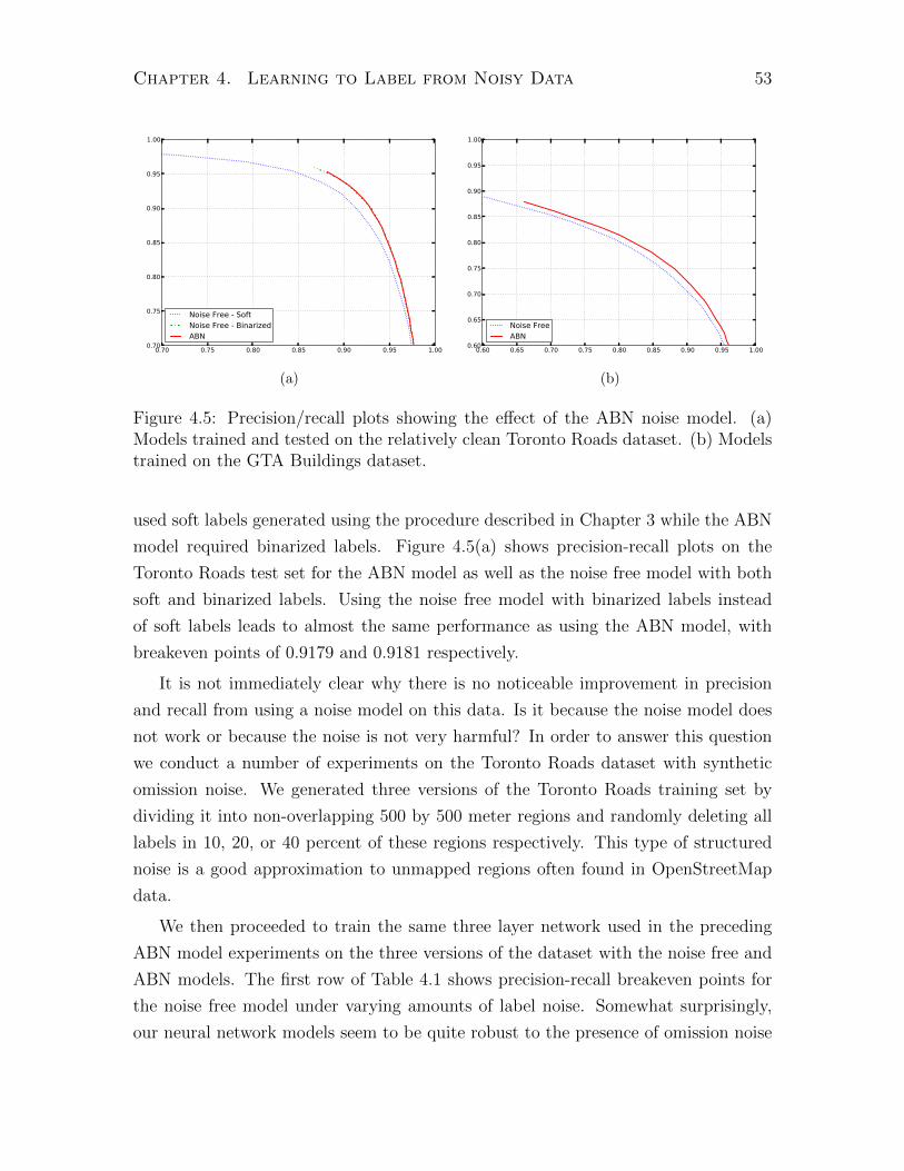
Chapter 4. Learning to Label from Noisy Data 53
0.70 0.75 0.80 0.85 0.90 0.95 1.000.70
0.75
0.80
0.85
0.90
0.95
1.00
Noise Free - SoftNoise Free - BinarizedABN
(a)
0.60 0.65 0.70 0.75 0.80 0.85 0.90 0.95 1.000.60
0.65
0.70
0.75
0.80
0.85
0.90
0.95
1.00
Noise FreeABN
(b)
Figure 4.5: Precision/recall plots showing the effect of the ABN noise model. (a)Models trained and tested on the relatively clean Toronto Roads dataset. (b) Modelstrained on the GTA Buildings dataset.
used soft labels generated using the procedure described in Chapter 3 while the ABN
model required binarized labels. Figure 4.5(a) shows precision-recall plots on the
Toronto Roads test set for the ABN model as well as the noise free model with both
soft and binarized labels. Using the noise free model with binarized labels instead
of soft labels leads to almost the same performance as using the ABN model, with
breakeven points of 0.9179 and 0.9181 respectively.
It is not immediately clear why there is no noticeable improvement in precision
and recall from using a noise model on this data. Is it because the noise model does
not work or because the noise is not very harmful? In order to answer this question
we conduct a number of experiments on the Toronto Roads dataset with synthetic
omission noise. We generated three versions of the Toronto Roads training set by
dividing it into non-overlapping 500 by 500 meter regions and randomly deleting all
labels in 10, 20, or 40 percent of these regions respectively. This type of structured
noise is a good approximation to unmapped regions often found in OpenStreetMap
data.
We then proceeded to train the same three layer network used in the preceding
ABN model experiments on the three versions of the dataset with the noise free and
ABN models. The first row of Table 4.1 shows precision-recall breakeven points for
the noise free model under varying amounts of label noise. Somewhat surprisingly,
our neural network models seem to be quite robust to the presence of omission noise
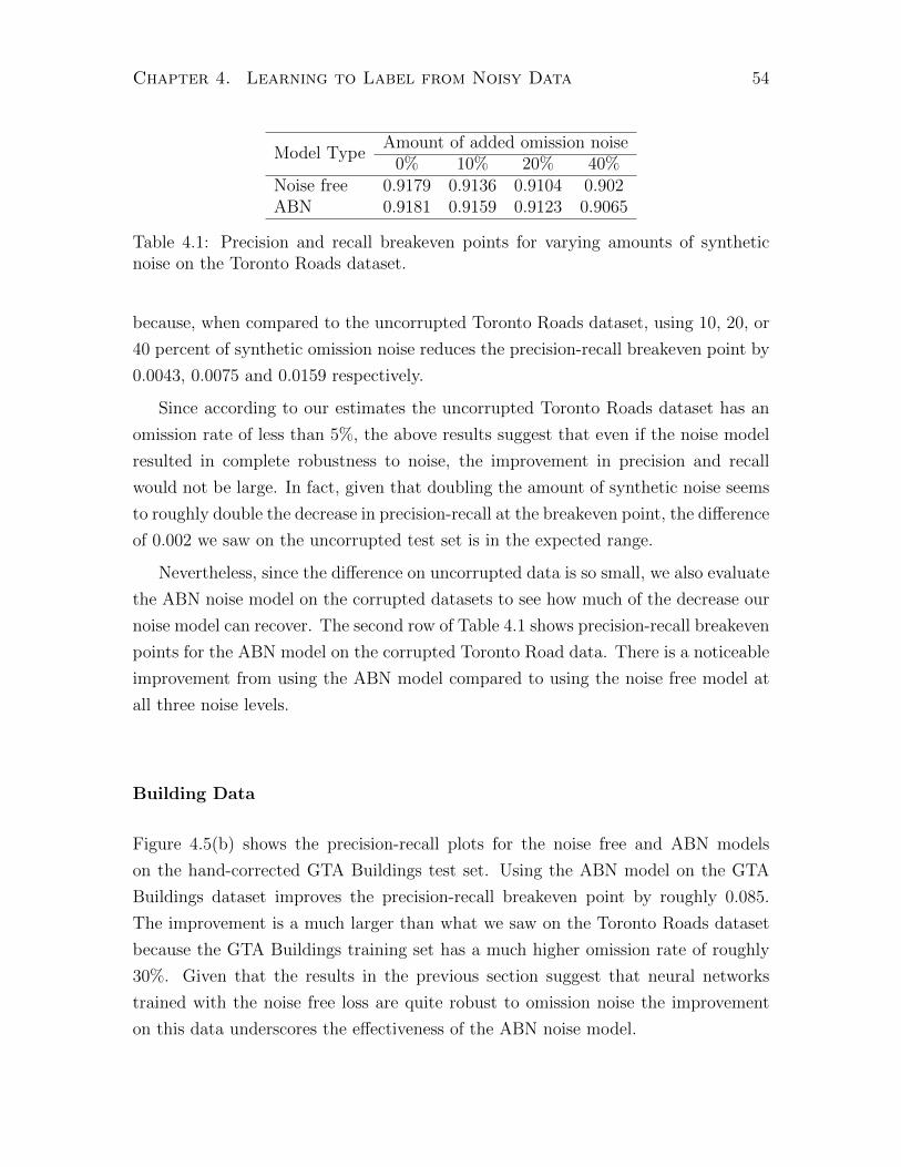
Chapter 4. Learning to Label from Noisy Data 54
Model TypeAmount of added omission noise
0% 10% 20% 40%Noise free 0.9179 0.9136 0.9104 0.902ABN 0.9181 0.9159 0.9123 0.9065
Table 4.1: Precision and recall breakeven points for varying amounts of syntheticnoise on the Toronto Roads dataset.
because, when compared to the uncorrupted Toronto Roads dataset, using 10, 20, or
40 percent of synthetic omission noise reduces the precision-recall breakeven point by
0.0043, 0.0075 and 0.0159 respectively.
Since according to our estimates the uncorrupted Toronto Roads dataset has an
omission rate of less than 5%, the above results suggest that even if the noise model
resulted in complete robustness to noise, the improvement in precision and recall
would not be large. In fact, given that doubling the amount of synthetic noise seems
to roughly double the decrease in precision-recall at the breakeven point, the difference
of 0.002 we saw on the uncorrupted test set is in the expected range.
Nevertheless, since the difference on uncorrupted data is so small, we also evaluate
the ABN noise model on the corrupted datasets to see how much of the decrease our
noise model can recover. The second row of Table 4.1 shows precision-recall breakeven
points for the ABN model on the corrupted Toronto Road data. There is a noticeable
improvement from using the ABN model compared to using the noise free model at
all three noise levels.
Building Data
Figure 4.5(b) shows the precision-recall plots for the noise free and ABN models
on the hand-corrected GTA Buildings test set. Using the ABN model on the GTA
Buildings dataset improves the precision-recall breakeven point by roughly 0.085.
The improvement is a much larger than what we saw on the Toronto Roads dataset
because the GTA Buildings training set has a much higher omission rate of roughly
30%. Given that the results in the previous section suggest that neural networks
trained with the noise free loss are quite robust to omission noise the improvement
on this data underscores the effectiveness of the ABN noise model.

Chapter 4. Learning to Label from Noisy Data 55
0.4 0.5 0.6 0.7 0.8 0.9 1.0Recall
0.4
0.5
0.6
0.7
0.8
0.9
1.0
Prec
isio
n
Noise Free - SoftNoise Free - BinarizedABNTABN
Figure 4.6: Precision/recall plots showing the effect of the TABN noise model. Themodels were trained on the smaller and much noisier Hamilton Roads dataset buttested on the cleaner Toronto Roads test set.
4.3.2 Registration Noise
In order to evaluate the robustness of the TABN model to registration noise, we per-
form experiments on the Hamilton Roads dataset. While the Toronto data contains
relatively few registration problems, with most road labels within one or two meters
of the true locations, road centerlines in the Hamilton Roads dataset are often more
than 5 meters away from their true locations. We train the ABN and TABN models
on the Hamilton training set and evaluate them on the Toronto Roads test set because
it is much cleaner.
Figure 4.6 shows precision-recall curves on the Toronto Roads test set for the
models trained on the Hamilton training set and demonstrates the clear advantage of
using the TABN robust loss function on this data. In addition to the TABN model,
we include results for the ABN model, as well as a noise free model trained on both
soft and binarized labels. As we saw on the road data, much of the improvement of
the ABN model over the noise free model can be attributed to using binarized labels.
Nevertheless, we get a substantial improvement in the precision recall curve from
training a network with the TABN model, improving the precision-recall breakeven
point by 0.0176 when compared to the ABN model.
It might seem surprising that the improvement from using the TABN model is so
much higher than from using the ABN model even on data with a lot of synthetic

Chapter 4. Learning to Label from Noisy Data 56
omission noise. The improvement is likely explained by two factors. First, neural
networks are likely less robust to registration errors than omission errors because while
omission errors may simply reduce the confidence of the neural network’s predictions,
registration errors can result in learning encouraging predictions that are entirely
wrong. The second factor explaining the effectiveness of the translational noise model
is the fact that under truly local registration errors it is possible for the TABN model
perfectly recover the true labels by translating the observed labels.
We further demonstrate the robustness of the TABN model to registration noise
by visualizing its predictions on noisy training data. Figure 4.7(a) shows an area
from the Hamilton Roads training set with the ground truth road locations overlaid
in red while Figure 4.7(b) shows the predictions of a model trained with the TABN
loss for the same area of the training set. The alignment between the predicted road
locations and their true locations is clearly much better than it is for the training
labels even though the training labels are what the model was trained to predict.
4.4 Conclusions and Discussion
We have shown that by using robust loss functions to train neural networks instead
of the standard negative log likelihood loss can provide some level of robustness to
label noise. Somewhat surprisingly, large amounts of omission noise do not seem
to significantly hurt the training of deep neural networks without a noise model,
although our ABN noise model does show across-the-board improvements. We also
saw that while the more structured registration noise is more harmful when no noise
model is used, it is actually easier to deal with when a translational noise model is
used.
While our noise models were designed specifically for the types of noise one faces
in aerial image labeling tasks, they can be easily modified to handle other types of
noise. For example, the translational noise model can be generalized to handle any
type of label noise for which we can write down a graphics program parameterized
with a single discrete transformation variable t. Any such graphics program G(m, t)
leads to a noise distribution
p(m|m, s, t) =
w2m∏
i=1
pABN(mi|G(m, t)i),

Chapter 4. Learning to Label from Noisy Data 57
that gives us some robustness to the transformation G. Rotations and shears are two
basic examples of transformations that can be handled in this manner.
One interesting extension of the ABN model is the addition of dependencies be-
tween pixels of the unobserved true map M. This modification would allow strong
disagreements with the ground truth in one part of a patch to influence weaker dis-
agreements in nearby parts of the patch. One way to achieve this effect is by placing
an MRF prior on M, leading to a combination of a CRF and our ABN noise model.
We will show how this model can be trained efficiently in the next chapter.

Chapter 4. Learning to Label from Noisy Data 58
(a)
(b)
Figure 4.7: Figure 4.7(a) Shows an area from the Hamilton Roads training set withthe training labels overlaid in red. Figure 4.7(b) shows the predictions on the trainingdata for a model trained with the TABN loss.

Chapter 5
Structured Prediction
So far we have only used unstructured models, meaning ones in which predictions
for individual pixels do not directly influence each other. Even though unstructured
models seem to be capable of achieving good performance on the tasks we have
considered, incorporating knowledge about the smoothness or shape of the predicted
objects should lead to even better performance. Indeed, as we discussed in Chapter 2,
incorporating structure into aerial and general image labeling methods has often led
to big improvements in accuracy and can be traced back to some of the earliest work
on the subject [Kettig and Landgrebe, 1976, Bischof et al., 1993, He et al., 2004,
Kluckner et al., 2009].
To gain some insight into the kinds of issues that we hope to address by incorporat-
ing structure we show sample predictions on the Toronto Roads and GTA Buildings
datasets in Figures 5.1(a) and 5.1(b) respectively. On road data, the most common
problems are disconnected blobs of road and gaps in the predicted road network.
A model that incorporates a connectedness constraint on the road network should
be able to avoid both types of errors. Similarly, the most common issues found in
predicted building maps are holes and disconnected blobs. Unlike with road data,
however, shape and layout are the cues that must be used to resolve these types of
errors. Incorporating structure into an image labeling approach by placing a smooth-
ness prior over the labels is likely to help address the issues with both road and
building detection. On top of this, incorporating higher level information, such as
shape, is likely to lead to further gains.
In this chapter, we aim to address the problem of incorporating rich dependencies
among the outputs of our models without sacrificing the ability to learn from large
59
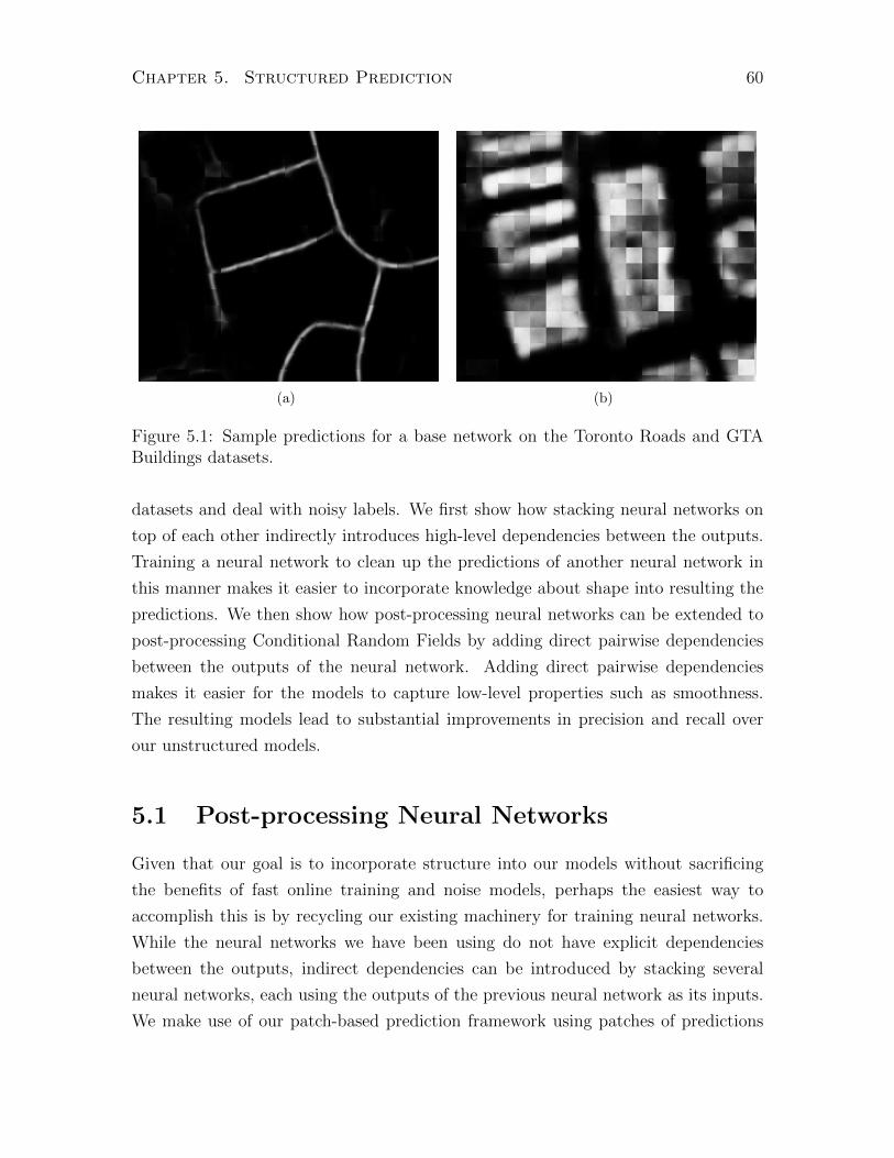
Chapter 5. Structured Prediction 60
(a) (b)
Figure 5.1: Sample predictions for a base network on the Toronto Roads and GTABuildings datasets.
datasets and deal with noisy labels. We first show how stacking neural networks on
top of each other indirectly introduces high-level dependencies between the outputs.
Training a neural network to clean up the predictions of another neural network in
this manner makes it easier to incorporate knowledge about shape into resulting the
predictions. We then show how post-processing neural networks can be extended to
post-processing Conditional Random Fields by adding direct pairwise dependencies
between the outputs of the neural network. Adding direct pairwise dependencies
makes it easier for the models to capture low-level properties such as smoothness.
The resulting models lead to substantial improvements in precision and recall over
our unstructured models.
5.1 Post-processing Neural Networks
Given that our goal is to incorporate structure into our models without sacrificing
the benefits of fast online training and noise models, perhaps the easiest way to
accomplish this is by recycling our existing machinery for training neural networks.
While the neural networks we have been using do not have explicit dependencies
between the outputs, indirect dependencies can be introduced by stacking several
neural networks, each using the outputs of the previous neural network as its inputs.
We make use of our patch-based prediction framework using patches of predictions
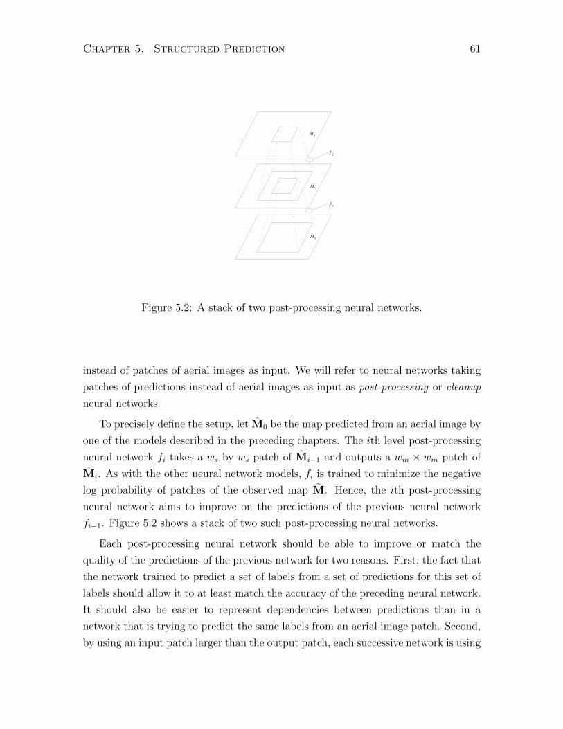
Chapter 5. Structured Prediction 61
M 0
M 1
M 2
f 1
f 2
Figure 5.2: A stack of two post-processing neural networks.
instead of patches of aerial images as input. We will refer to neural networks taking
patches of predictions instead of aerial images as input as post-processing or cleanup
neural networks.
To precisely define the setup, let M0 be the map predicted from an aerial image by
one of the models described in the preceding chapters. The ith level post-processing
neural network fi takes a ws by ws patch of Mi−1 and outputs a wm × wm patch of
Mi. As with the other neural network models, fi is trained to minimize the negative
log probability of patches of the observed map M. Hence, the ith post-processing
neural network aims to improve on the predictions of the previous neural network
fi−1. Figure 5.2 shows a stack of two such post-processing neural networks.
Each post-processing neural network should be able to improve or match the
quality of the predictions of the previous network for two reasons. First, the fact that
the network trained to predict a set of labels from a set of predictions for this set of
labels should allow it to at least match the accuracy of the preceding neural network.
It should also be easier to represent dependencies between predictions than in a
network that is trying to predict the same labels from an aerial image patch. Second,
by using an input patch larger than the output patch, each successive network is using

Chapter 5. Structured Prediction 62
(a) (b)
Figure 5.3: Predictions of post-processing neural networks for the areas shown inFigure 5.1.
information extracted from a larger and larger area of the aerial image as input. This
allows post processing networks to propagate confidence along the predicted maps.
There are two main advantages to using post-processing neural networks for in-
corporating structure into the predictions. One immediate benefit is the fact that the
robust losses from Chapter 4 can be used to train post-processing networks without
modification. Two, given the fact that neural networks are universal approxima-
tors, at least in theory, post-processing neural networks are capable of representing
arbitrary dependencies between input predictions and output label probabilities.
As we discussed in Chapter 2, trained classifiers have been used for post-processing
in the past. For example, Bischof et al. [1993] trained logistic regression models to
remove salt and pepper noise from aerial image classification results. In the remainder
of this section, we evaluate different types of post-processing neural network archi-
tectures, including shallow, single hidden layer networks and networks with multiple
levels of local or convolutional features, on road and building detection tasks. Our
results confirm the effectiveness of this simple approach to doing structured predic-
tion.
5.1.1 Results
To evaluate different post-processing neural network architectures, we first trained
two copies of a three layer locally connected network on the Toronto Roads and

Chapter 5. Structured Prediction 63
0.70 0.75 0.80 0.85 0.90 0.95 1.00Recall
0.70
0.75
0.80
0.85
0.90
0.95
1.00Pr
ecis
ion
Base networkLocal post processing networkFully connected post processing netwrokConvolutional post processing network
(a)
0.50 0.55 0.60 0.65 0.70 0.75 0.80 0.85 0.90 0.95 1.00Recall
0.50
0.55
0.60
0.65
0.70
0.75
0.80
0.85
0.90
0.95
1.00
Prec
isio
n
Base networkLocal post processing networkFully connected post processing netwrokConvolutional post processing network
(b)
Figure 5.4: Precision/recall plots showing the effect of cleanup with different networkarchitectures. (a) Post processing on the Toronto Roads dataset. (b) Post processingon the GTA Buildings dataset.
GTA Buildings datasets. These base networks used aerial image patches as input
and were trained for 20 epochs, at which point validation precision and recall stop
improving noticeably. We then trained three different post-processing neural network
architectures to predict 16 by 16 map patches from 64 by 64 patches of predictions
of the base networks on each dataset.
The first architecture is a neural network with a single fully-connected hidden
layer with 4096 hidden units. The second architecture is a two-layer locally-connected
network with 64 filters of size 12 by 12 with stride 1 in the first hidden layer and 256
filters of size 4 by 4 with stride 2 in the second hidden layer. Finally the third
architecture is a convolutional version of the second architecture. The hidden layers
in all three architectures consisted of rectified linear units.
Figures 5.4(a) and 5.4(b) show the precision-recall curves for the models we com-
pared on the Toronto Roads and GTA Buildings datasets respectively. All three
post-processing network architectures give a substantial improvement in precision
and recall over the base networks, but the difference between different architectures
themselves is quite small. We found this to be a general trend – post processing leads
to a substantial improvement over the base network, but there is little difference in
performance between different architecture choices such as the sizes and types of the
hidden layers.
In order to visually demonstrate the improvement in the predictions of the post-
Chapter 5. Structured Prediction 64
processing networks over the base networks, Figure 5.3 shows the predictions of the
best post-processing networks on the areas for which base network predictions are
shown in Figure 5.1. The post-processing network suppressed the disconnected blobs
of road present in the base network predictions in Figure 5.1(a) and filled in most of
the gaps in the road network. The network essentially learns to propagate confident
predictions along the map while respecting the constraints of the predicted road
network. A similar effect can be seen in the building predictions, where the post-
processing network propagates confident predictions while respecting the constraints
on building shape it has learned from the data.
5.2 Conditional Random Fields
One drawback of post-processing neural networks is that they do not incorporate
prior knowledge by explicitly coupling the model outputs and instead attempt to
learn all dependencies from data. While, as we showed in the previous section, this
approach is able to learn useful dependencies between outputs, post processing neural
networks fail to model local smoothness, which is the strongest local dependence.
Though stacking multiple post-processing neural networks on top of one another
might eventually come close to modeling smoothness really well, it may be easier and
more effective to incorporate such strong prior knowledge directly into the model.
In this section, we explore extending our deep neural networks to deep Conditional
Random Fields (CRFs) by adding explicit dependencies between outputs of a neural
network. In particular, we add a smoothness term between neighbouring pixels to
our model, removing the need to learn smoothness from the data. Using the resulting
models for post-processing leads to substantial improvements over unstructured, post-
processing neural networks.
5.2.1 Model Description
Following the discussion of Chapter 2, an image labeling CRF is simply a Markov
Random Field over the set of pixel labels, which is globally conditioned on the image.
In the context of our patch-based labeling framework, the observed map distribution
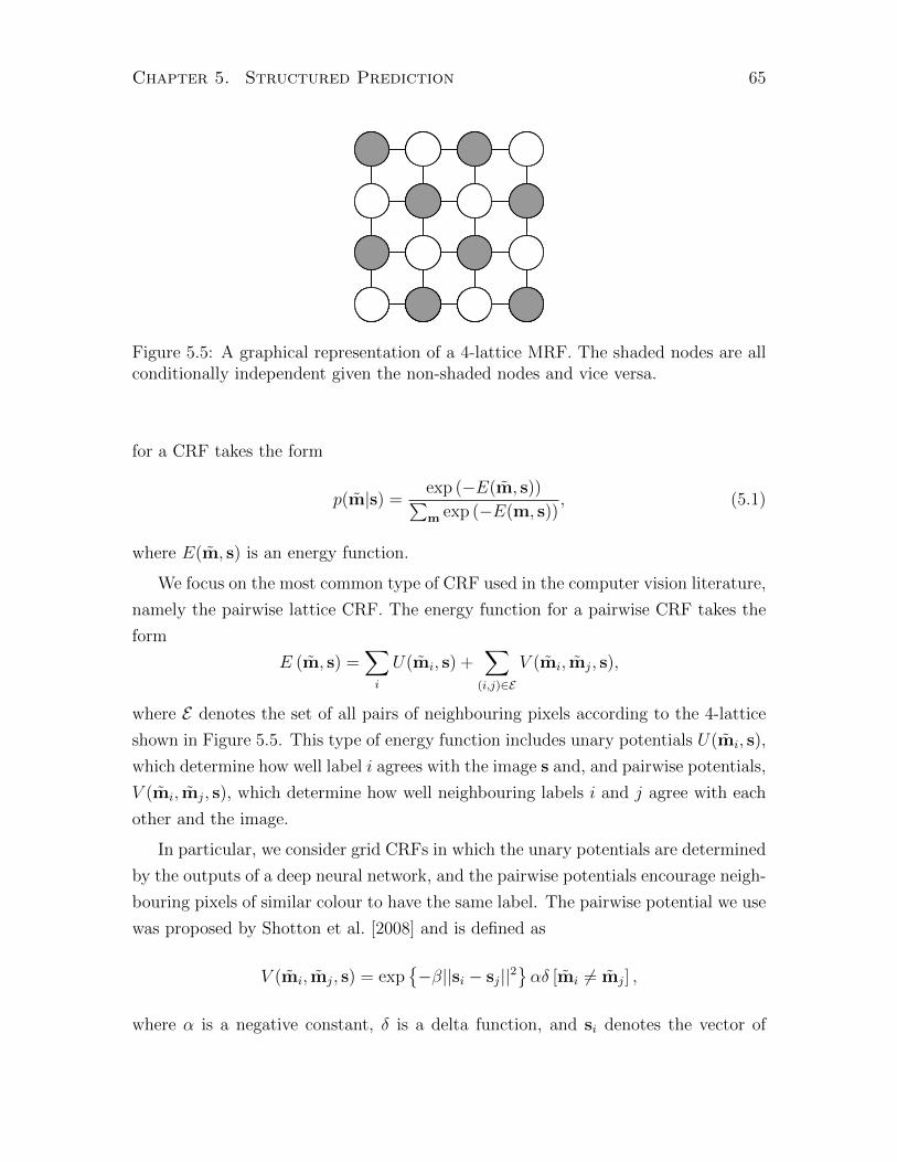
Chapter 5. Structured Prediction 65
Figure 5.5: A graphical representation of a 4-lattice MRF. The shaded nodes are allconditionally independent given the non-shaded nodes and vice versa.
for a CRF takes the form
p(m|s) =exp (−E(m, s))∑m exp (−E(m, s))
, (5.1)
where E(m, s) is an energy function.
We focus on the most common type of CRF used in the computer vision literature,
namely the pairwise lattice CRF. The energy function for a pairwise CRF takes the
form
E (m, s) =∑i
U(mi, s) +∑
(i,j)∈EV (mi, mj, s),
where E denotes the set of all pairs of neighbouring pixels according to the 4-lattice
shown in Figure 5.5. This type of energy function includes unary potentials U(mi, s),
which determine how well label i agrees with the image s and, and pairwise potentials,
V (mi, mj, s), which determine how well neighbouring labels i and j agree with each
other and the image.
In particular, we consider grid CRFs in which the unary potentials are determined
by the outputs of a deep neural network, and the pairwise potentials encourage neigh-
bouring pixels of similar colour to have the same label. The pairwise potential we use
was proposed by Shotton et al. [2008] and is defined as
V (mi, mj, s) = exp{−β||si − sj||2
}αδ [mi 6= mj] ,
where α is a negative constant, δ is a delta function, and si denotes the vector of

Chapter 5. Structured Prediction 66
colour values for pixel i. When the pixels si and sj are not similar, the exponential
term of the potential will be close to 0, making a negligible contribution to the energy
for all possible labels mi and mj. When the pixels si and sj are similar, however,
the exponential term will be close to 1, which means that the penalty of α will be
added to the energy when mi and mj are different. This type of potential directly
encourages smoothness of the labels in homogeneous regions of the image. The energy
function for a CRF with these types of potentials can be expressed as
E (m, s) = −∑i
(mi log fi(s)− (1− mi) log(1− fi(s))
−∑j∈N(i) exp {−β||si − sj||2}αδ [mi 6= mj]),
where fi(s) is the ith output of the neural network.
This basic pairwise CRF model can be extended in a number of different ways. For
example, Kohli et al. [2009] build a model that combines multiple oversegmentations of
an image and obtain more fine-grained segmentations by using higher order potentials
to encourage label consistency within superpixels of the oversegmentations. Gould
et al. [2008] extend the basic model with a prior over the relative locations of different
object types. We do not use these types of extensions and instead hope to capture
some of the same dependencies by stacking models on top of each other. Since the
unary potentials of our model are determined by the outputs of a deep neural network,
the model could conceivably be able to reason about the relative locations of predicted
objects whenever it is used for post-processing. We also hope that the use of a deep
neural network for the unary potentials will lead to more fine-grained segmentations
compared to models with less powerful unary potentials, despite the fact that we use
a simple smoothing term.
5.2.2 Predictions and Inference
The standard way of making predictions with a CRF is by finding the labeling with
the highest probability under the model. More precisely, we would like to find the so
called MAP labeling mMAP , defined as
mMAP = arg maxm
p(m|s).
Chapter 5. Structured Prediction 67
While the problem of finding the MAP labeling in general CRFs, known as MAP
inference, is known to be NP-hard, there are broad classes of CRFs for which efficient
exact MAP inference is possible. Pairwise CRFs in which the pairwise potentials
satisfy a condition known as submodularity are one such class. Under our formulation,
submodularity corresponds to the condition
V (0, 1, s) + V (1, 0, s) ≤ V (0, 0, s) + V (1, 1, s). (5.2)
For any model satisfying this condition, the MAP labeling can be found in polynomial
time using graph cuts [Greig et al., 1989]. Conveniently, the submodularity condition
simply states that the model should favour smoothness in the labels and it is satisfied
by our models for all non-positive values of α.
Despite the fact that efficient and exact MAP inference for our model is possible
using graph cuts, it is not a good choice in this setting because it produces a hard 0/1
labeling. The resulting labeling leads to a single pair of precision and recall values,
making it impossible to trade off one for the other by choosing a threshold. Indeed, we
found that graph cut inference leads to predictions with high precision and moderate
recall, which may not be desirable. For this reason, we do not use MAP inference
and instead perform marginal inference where the goal is to compute the marginals
p(mi|s) for all pixels i. Computing the marginals allows us to trade off precision
and recall against each other by choosing a threshold and using it to produce a hard
assignment from the marginal probabilities.
We experimented with two types of marginal inference: mean field inference based
on a fully-factored distribution and loopy belief propagation. While the two types of
inference led to nearly identical precision-recall curves, mean field inference is both
faster and more straight forward to implement, so we present it here in detail.
Mean field inference involves finding the fully-factored distribution q that is closest
to p(m|s) in terms of KL-divergence. More precisely, the mean field approximation
of p(m|s) is the distribution q defined as
q = arg minq∗
KL (q∗||p(m|s)) such that q∗(m) =∏i
q∗i (mi),
Not surprisingly, it is rarely possible to find a closed form solution to this variational
minimization problem unless the distribution being approximated is in the class of

Chapter 5. Structured Prediction 68
approximating distributions, which would entirely defeat the purpose of finding an
approximation. Instead, solving for q typically leads to an expression for each qi in
terms of the other q’s, which can in turn be used to iteratively update the q’s starting
from some initial guess until a stationary point is reached.
In order to derive the mean field approximation to p(m|s) we first write out KL-
divergence between q and p(m|s) and separate out its dependence on a single term
qj. Hence,
KL(q||p(m|s)) =∑m
q(m) logp(m|s)
q(m)
=∑i
∑mi
(∏i
qi(mi)
)(log p(m|s)−
∑i
log qi(mi)
)
=∑mj
qj(mj)∑mi6=j
[(∏i 6=j
qi(mi)
)(log p(m|s)−
∑k
log qk(mk)
)]=
∑mj
qj(mj)∑mi6=j
[(∏i 6=j
qi(mi)
)log p(m|s)
]−∑mj
qj(mj) log qj(mj) + C,
where C is a constant that does not depend on qj. At this point, we can take partial
derivatives of KL(q||p) with respect to qj(mj = 0) and qj(mj = 1) set them to 0 to
obtain that
qj(mj) = exp (Eqi,i 6=j [log p(m|s)]) /Zj,
where Zj is a normalizing constant. This gives us a set of consistency equations that
must hold for the distribution q that minimizes KL(q||p).While this is not a closed form solution for the best possible approximating dis-
tribution q, we can find a fixed point for these equations by iteratively updating the
qi’s using the consistency equations starting with some initial guess, with convergence
guaranteed. Since updating one qi at a time does not lend itself to easy parallelization
we instead perform damped parallel updates. While convergence to a fixed point is
no longer guaranteed, we find that the procedure works well in practice. We pro-
vide the mean field inference procedure for CRFs with the energy function defined in
Equation 5.2 as Algorithm 1.

Chapter 5. Structured Prediction 69
Result: Approximate marginals qMF
Initialize q(0)i to 0.5 for all i
for t = 1, . . . , T doCompute the iterated q∗i ’s according to:
log q∗j (mj) = mi ln fj(s) + (1− mi) ln(1− fj(s)) +∑k∈N(j)
∑mkq(t−1)k (mk)V (mj, mk, s)
Compute the updated qi’s according to:
q(t)j (mj) = γq∗j (mj) + (1− γ)q
(t−1)j (mj)
end
return q(T )
Algorithm 1: Mean-Field Inference for Grid CRFs
One thing to note is that due to the 4-lattice structure of the CRF the update
equation for each pixel is a sparse computation involving only its 4 neighbours. By
breaking down the computation into four separate steps, one for each direction of
neighbours, it is possible to vectorize this update and perform it in parallel for an
entire minibatch.
The mean-field inference procedure has two free parameters: the number of infer-
ence steps T and the damping factor γ. We experimented with a few settings of the
parameters and found that using T = 10 and γ = 0.5 seemed to work well. We used
these parameter values for both training and testing in all experiments where mean
field inference was used.
Figure 5.6 shows the first six steps q(1), . . . , q(6) of this mean field inference proce-
dure for a CRF trained on the GTA Buildings dataset. While some boundary artifacts
are still present, the inference procedure does a good job of removing some of them
by propagating confident predictions.
5.2.3 Learning
Our CRF has two sets of parameters – the parameters of the neural network deter-
mining the unary potentials and the parameters α and β of the pairwise potential.
We learn the two sets of parameters separately, which is a common practice in the
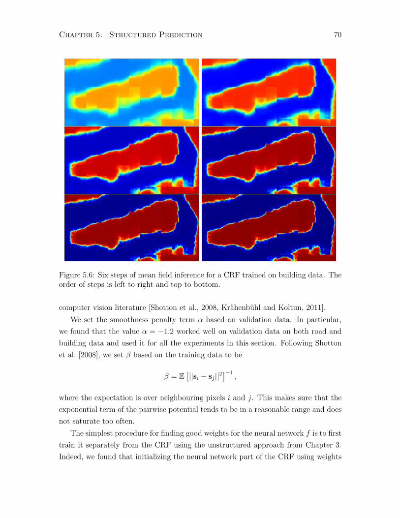
Chapter 5. Structured Prediction 70
Figure 5.6: Six steps of mean field inference for a CRF trained on building data. Theorder of steps is left to right and top to bottom.
computer vision literature [Shotton et al., 2008, Krahenbuhl and Koltun, 2011].
We set the smoothness penalty term α based on validation data. In particular,
we found that the value α = −1.2 worked well on validation data on both road and
building data and used it for all the experiments in this section. Following Shotton
et al. [2008], we set β based on the training data to be
β = E[||si − sj||2
]−1,
where the expectation is over neighbouring pixels i and j. This makes sure that the
exponential term of the pairwise potential tends to be in a reasonable range and does
not saturate too often.
The simplest procedure for finding good weights for the neural network f is to first
train it separately from the CRF using the unstructured approach from Chapter 3.
Indeed, we found that initializing the neural network part of the CRF using weights

Chapter 5. Structured Prediction 71
of a separately trained neural network led to good results. Since this way of learning
the unary potentials of a CRF does not make use of the pairwise terms, we explored
the possibility of finetuning the neural network determining the unary potentials of
a CRF using gradient descent on the CRF negative log likelihood.
For a single training case, the partial derivative of the negative log likelihood of a
general CRF with respect to a parameter θ is given by
−∂ log p(m|s, θ)∂θ
= ∂E(m,s)∂θ
−∑m p(m|s, θ)∂E(m,s)∂θ
= ∂E(m,s)∂θ
− Ep(m|s)[∂E(m,s)
∂θ
].
The expression for the partial derivative consists of two terms. The first term, known
as the positive term, is simply the partial derivative of the energy with respect to
the parameter, and is straightforward to compute for most models, including ours.
The second term, known as the negative term, is the partial derivative of the log
partition function and takes the form of an expected value of the partial derivative
of the energy with respect to the model distribution p(m|s). Since the negative term
requires summing over a number of terms exponential in the number of pixels, it
is generally intractable to compute, even for a model as simple as a 4-lattice CRF,
forcing one to use approximate learning methods.
Broadly speaking, approximate learning methods for models with intractable par-
tition functions can be divided into stochastic and deterministic approximations. We
experimented with learning the parameters of f using both types of approximations,
which we now discuss in greater detail.
Deterministic approximations
We considered the broad category of deterministic approximation methods which
involves replacing the expectation with respect to the model distribution p(m|s) with
an expectation over some tractable distribution q. In models where MAP inference
is tractable, a popular choice for q is a point mass distribution with all of its mass
placed on the MAP prediction mMAP . While it would be interesting to experiment
with using MAP inference during learning we chose to use the fully factored mean
field approximation to p(m|s) as the distribution q because the computation can be
easily parallelized.

Chapter 5. Structured Prediction 72
Using the approximation
−∂ log p(m|s)
∂θ≈ ∂E (m, s)
∂θ− EqMF
[∂E (m, s)
∂θ
],
where qMF is the result of mean field inference described in Section 5.2.2, we get the
intuitively pleasing result that
−∂ log p(m|s)
∂ai(s)≈ mi − qMF
i (m), (5.3)
where ai(s) is the total input to the output unit for the ith pixel. Hence, according to
the approximations we have used, the partial derivative of the negative log likelihood
with respect to the activation of a single unit ai(s) is just the difference between the
observed label and the probability of the observed label being 1 according to mean
field inference. The partial derivatives of the loss with respect to the parameters of the
neural network f can be easily computed from Equation 5.3 using backpropagation.
Our attempts to learn the unary potentials of the CRF defined by the neural
network f using the above approach were not successful. All models finetuned with
this approach were considerably worse than the neural networks they were initialized
with. The problem likely stems from the fact that the mean field approximation
of the model distribution tends to be overconfident because it converges on a single
mode [Bishop, 2006]. It is common for the entries of q to be very close to 0 whenever
the neural network assigns a low probability of an object of interest being present.
This has the effect of driving up the biases of the neural network and leads to an
increased false positive rate.
Stochastic approximations
Stochastic approximation techniques rely on using Monte Carlo methods for approx-
imating the expectation in the negative term. In cases where it is easy to efficiently
draw samples from the model distribution, sampling-based techniques can be used to
obtain an unbiased estimate of the negative term. Since probabilistic models with
intractable partition functions, including the types of CRFs we consider, are usually
difficult to sample from, approximate sampling techniques must be used.
We experimented with approximating the negative term expectation using a Markov
chain whose stationary distribution is the model distribution p(m|s). The transition

Chapter 5. Structured Prediction 73
operator of the Markov chain we used for our model is a block Gibbs sampler with
two groups defined using a checker board pattern, as shown in Figure 5.5. All the
shaded nodes can be updated in parallel given all the unshaded nodes and vice versa,
allowing us to update all nodes in just two block Gibbs updates. By running the
Markov chain until it reaches equilibrium, we could obtain samples from the model
p(m|s) and use them to approximate the negative term expectation. Unfortunately
this approach is impractical because it takes a long time to reach equilibrium.
One alternative is to use Contrastive Divergence (CD) learning [Hinton, 2002],
which initializes the Markov chain at the data m and runs the Markov chain for a
small number of steps instead of running until convergence. We found that finetuning
a CRF using CD actually made the predictions worse. This confirms our earlier
finding that CD may not work well for training conditional models [Mnih et al., 2011]
where the Markov chain mixes slowly. Intuitively, CD training lowers the energy of
the observed data and raises the energy of the regions near the true data. This may
not work well for a conditional model because test time inference starts away from
the true data and may never reach the regions of the state space explored by CD at
training time.
We experimented with a number of alternatives to standard CD training and
found that we could successfully finetune a CRF using CD where the Markov chain
in the negative phase run at temperature 2 instead of 1. Running the Markov chain
at the higher temperature improved mixing in the chain. Additionally, we found that
using a different value of the pairwise smoothness penalty term α at training time also
improved mixing of the chain leading to even better finetuning results. While using
the value of α = −1.2 works well at test time, it leads to rather rigid smoothness
constraints on the labels which make it difficult for our Gibbs sampler to make large
moves. Thus our finetuning procedure used CD with the negative chain running at
temperature 2 for 5 steps and the pairwise penalty term set to −0.6. While it might
be possible to use CD training without any model modifications by using a better
sampler such as Swendsen-Wang [Swendsen and Wang, 1987], we did not explore this
possibility.

Chapter 5. Structured Prediction 74
Model Base Post-processingnn 0.7985 0.8176crf 0.8144 0.8343Finetuned crf 0.8296 0.8351Finetuned nn crf 0.8268 0.8345
Table 5.1: Precision and recall breakeven points for different base and cleanup modelson the GTA Buildings dataset.
5.2.4 Results
Due to the fact that smoothness is more important for building detection than road
detection we evaluate the proposed CRF model on the GTA Buildings dataset. We
evaluate two types of models – base models taking aerial images as input and post-
processing models using the outputs of a neural network as the input.
Table 5.1 shows precision-recall breakeven point values on the GTA Buildings
dataset for neural networks as well as CRFs trained in different ways. nn denotes a
deep neural network trained using the procedure described in Chapter 3, while crf
denotes a CRF whose neural network weights were initialized with the weights of
nn. The parameters of this model were not finetuned. The model Finetuned crf
corresponds to initializing a CRF with the weights of crf and finetuning it for two
epochs by optimizing the CRF likelihood using Contrastive Divergence. Finally, the
model Finetuned nn crf is a CRF whose neural network weights were obtained
by training nn for two more epochs using the standard neural net likelihood. We
included Finetuned nn crf to see if there is a benefit from finetuning a CRF using
the CRF likelihood as opposed to just training the neural network part longer using
the unstructured neural network likelihood.
CRFs trained using all three procedures substantially outperform nn. For both
base and post-processing models, simply placing an MRF over the outputs of a neural
network to turn it into a CRF, which is the difference between nn and crf, improves
precision-recall breakeven points by roughly 0.015. We also see that while finetuning a
CRF using the CRF likelihood leads to a slightly bigger improvement in performance
than simply training the neural network longer, the difference between these two
methods is too small to be conclusive.
It is also interesting to note that post-processing CRFs are the best performing
models, outperforming both post processing neural networks and base CRFs. This
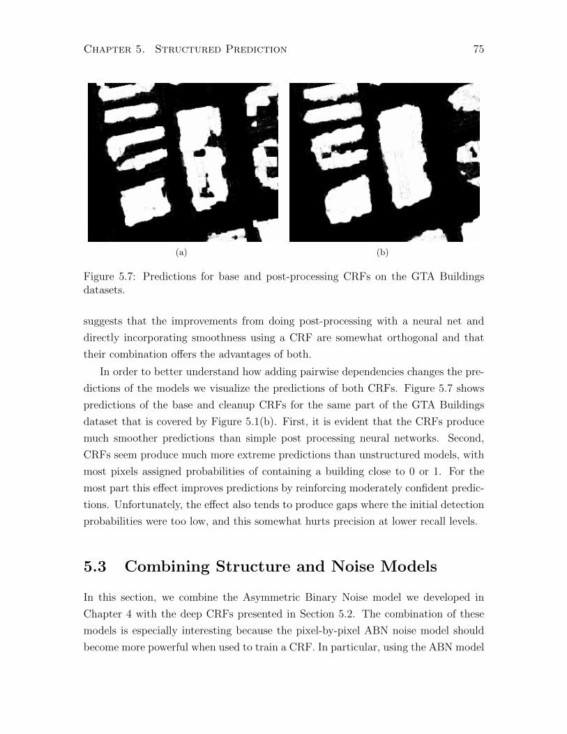
Chapter 5. Structured Prediction 75
(a) (b)
Figure 5.7: Predictions for base and post-processing CRFs on the GTA Buildingsdatasets.
suggests that the improvements from doing post-processing with a neural net and
directly incorporating smoothness using a CRF are somewhat orthogonal and that
their combination offers the advantages of both.
In order to better understand how adding pairwise dependencies changes the pre-
dictions of the models we visualize the predictions of both CRFs. Figure 5.7 shows
predictions of the base and cleanup CRFs for the same part of the GTA Buildings
dataset that is covered by Figure 5.1(b). First, it is evident that the CRFs produce
much smoother predictions than simple post processing neural networks. Second,
CRFs seem produce much more extreme predictions than unstructured models, with
most pixels assigned probabilities of containing a building close to 0 or 1. For the
most part this effect improves predictions by reinforcing moderately confident predic-
tions. Unfortunately, the effect also tends to produce gaps where the initial detection
probabilities were too low, and this somewhat hurts precision at lower recall levels.
5.3 Combining Structure and Noise Models
In this section, we combine the Asymmetric Binary Noise model we developed in
Chapter 4 with the deep CRFs presented in Section 5.2. The combination of these
models is especially interesting because the pixel-by-pixel ABN noise model should
become more powerful when used to train a CRF. In particular, using the ABN model
Chapter 5. Structured Prediction 76
to train a CRF should allow nearby disagreements of the neural network predictions
with the ground truth to reinforce each other. This effect does not exist when the
ABN model is used to train a neural network because the negative log likelihood
decomposes over pixels due to the lack of direct dependencies between different labels.
5.3.1 The model
We recall from Chapter 4 that in order to deal with omission noise we defined the
following two-stage generative model of the data:
1. Generate the true, uncorrupted and unobserved map m from the aerial image
s according to a data distribution p(m|s).
2. Generate the corrupted observed map m from the true map m according to a
noise distribution p(m|m).
When the noise distribution is specified by the asymmetric binary noise model, this
generative process leads to the following observed map distribution:
p(m|s) =∑m
(∏i
p(mi|mi)
)p(m|s).
In Chapter 4, the true map distribution p(m|s) was specified using a neural net and
factored over pixels, which led to a p(m|s) that also factored over pixels. Here, the
true map distribution is specified by a CRF, which means that the observed map
distribution no longer factors over pixels. We will refer to this model as the CRF-
ABN model. While coupling the pixels in this manner makes learning more difficult,
it gives the model some interesting properties. Figure 5.8 shows the difference in the
inferred true map m between the ABN and CRF-ABN models. In particular, one
can see how nearby disagreements reinforce each other in the CRF-ABN model and
not in the ABN model.
5.3.2 Inference
Since the noise model only has an effect at training time, the test time inference prob-
lem for the CRF-ABN model is the same as for the plain CRF model from Section 5.2.
Namely, the goal is to compute the marginals p(mi|s) for making predictions from
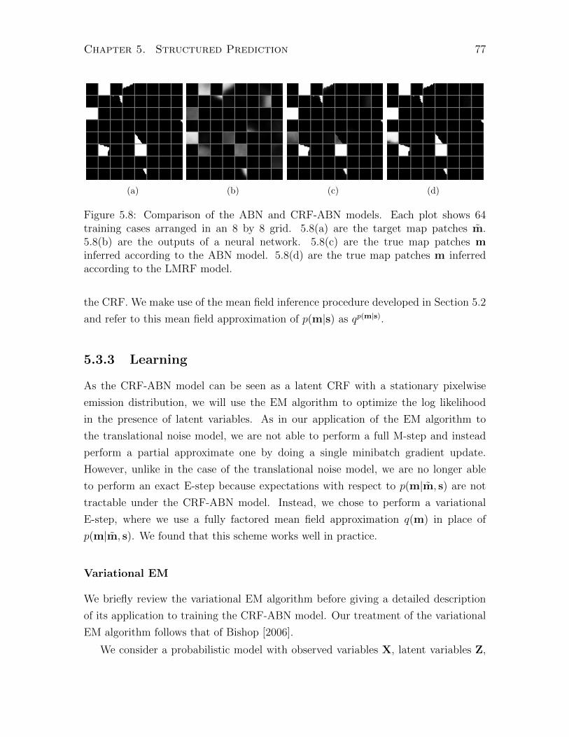
Chapter 5. Structured Prediction 77
(a) (b) (c) (d)
Figure 5.8: Comparison of the ABN and CRF-ABN models. Each plot shows 64training cases arranged in an 8 by 8 grid. 5.8(a) are the target map patches m.5.8(b) are the outputs of a neural network. 5.8(c) are the true map patches minferred according to the ABN model. 5.8(d) are the true map patches m inferredaccording to the LMRF model.
the CRF. We make use of the mean field inference procedure developed in Section 5.2
and refer to this mean field approximation of p(m|s) as qp(m|s).
5.3.3 Learning
As the CRF-ABN model can be seen as a latent CRF with a stationary pixelwise
emission distribution, we will use the EM algorithm to optimize the log likelihood
in the presence of latent variables. As in our application of the EM algorithm to
the translational noise model, we are not able to perform a full M-step and instead
perform a partial approximate one by doing a single minibatch gradient update.
However, unlike in the case of the translational noise model, we are no longer able
to perform an exact E-step because expectations with respect to p(m|m, s) are not
tractable under the CRF-ABN model. Instead, we chose to perform a variational
E-step, where we use a fully factored mean field approximation q(m) in place of
p(m|m, s). We found that this scheme works well in practice.
Variational EM
We briefly review the variational EM algorithm before giving a detailed description
of its application to training the CRF-ABN model. Our treatment of the variational
EM algorithm follows that of Bishop [2006].
We consider a probabilistic model with observed variables X, latent variables Z,

Chapter 5. Structured Prediction 78
and a joint distribution p(X,Z|θ). The goal is to optimize the log likelihood
log p(X|θ) = log∑Z
p(X,Z|θ),
and we assume that this is difficult due to the presence of the sum inside the logarithm.
Additionally, we assume that maximizing the complete log likelihood log p(X,Z|θ) is
straightforward with respect to θ.
The central idea behind the EM algorithm is decomposing the log likelihood as
log p(X|θ) = L(q, θ) +KL(q||p(Z|X)),
where q is a distribution defined over the latent variables Z, and
L(q, θ) =∑Z
q(Z) logp(X,Z|θ)q(Z)
.
This decomposition holds for any choice of distribution q, and because the KL-
divergence KL(q||p) is nonnegative, the term L(q, θ) is a lower bound on the log
likelihood log p(X|θ).
The EM algorithm maximizes the log likelihood log p(X|θ) by performing an al-
ternating maximization of the lower bound L(q, θ). In the E-step, L is maximized
with respect to q. Since L is bounded from above by log p(X|θ) and KL(q||p) is 0 if
and only if q = p, L attains its maximum with respect to q at q = p(Z|X). In the
second step of the alternating minimization, the M-step, L is maximized with respect
to the model parameters θ, which corresponds to maximizing∑Z
q(Z) log p(X,Z|θ). (5.4)
Since L is a lower bound on the log likelihood, increasing L is guaranteed to increase
the log likelihood when the bound is tight.
Unfortunately, maximizing the quantity in Equation 5.4 for the choice q(Z) =
p(Z|X, θ) is intractable for many models of interest. The key idea behind the vari-
ational EM algorithm is to restrict the maximization performed in the E-step to a
class of distributions for which maximizing the quantity in Equation 5.4 is tractable.

Chapter 5. Structured Prediction 79
One common choice for q is the mean field approximation which is defined as
qMF = arg maxq(Z)L(q, θ) such that q(Z) =
∏i
qi(Zi)
and corresponds to restricting the maximization of L to the class of fully factored
distributions q.
While the EM algorithm always improves the log likelihood unless a local opti-
mum has already been reached, since the E-step in the variational EM algorithm
corresponds to a partial maximization of L, the M-step is no longer guaranteed to
improve the log likelihood. Nevertheless, both steps of the variational EM algorithm
increase L when possible, and since L is a lower bound on the log likelihood , varia-
tional EM tends to increase the log likelihood in practice.
We now describe our variational EM algorithm for training the CRF-ABN model.
M-step:
The goal of the M-step is to maximize L with respect to the parameter vector θ. Since
we are training a nonlinear model, we opt for a partial approximate M-step in which
we do a single minibatch update of stochastic gradient descent on the parameters θ.
Following the approaches used to learn the parameters of the ABN model in Chapter 4
and the CRF parameters in Section 5.2 we use gradient information only to learn the
parameters of the neural network f and use a validation set to learn the pairwise
term of the MRF and the noise model parameters.
In order to derive the required update, we take the partial derivative of the vari-
ational lower bound L with respect to a single parameter θ and obtain
∂L(q, θ)
∂θ=
∂
∂θ
∑m
q(m) log p(m|s) (5.5)
= −(∑
m
q(m)
(∂E(m, s)
∂θ− Ep(m|s)
[∂E(m, s)
∂θ
]))(5.6)
= −(Eq(m)
[∂E(m, s)
∂θ
]− Ep(m|s)
[∂E(m, s)
∂θ
]), (5.7)
by removing terms that do not depend on θ and rewriting summations as expectations
where possible. The first term in Equation 5.7 is an expectation of the CRF’s energy
Chapter 5. Structured Prediction 80
derivative with respect to the mean field approximation q and is straightforward to
evaluate. The second term in the same expression is the expectation of the CRF’s
energy derivative with respect to the CRF’s model distribution p(m|s) and, as we
saw in Section 5.2 is intractable for our model. Since we already addressed the issue
of approximating this term, we follow the approach from Section 5.2. In particular
we use CD with the Markov chain running at temperature 2 and, as before, we also
set the pairwise penalty term to −0.6 at training time in order to further improve
mixing of the Markov chain.
Combining the above approximation with Equation 5.7 we obtain that the ap-
proximate partial derivative of L with respect to the activation ai of the ith output
unit of the neural network f is given by
∂L(q, θ)
∂ai≈ −
(Eq(m)
[∂E(m, s)
∂ai
]− Ep(m|s)
[∂E(m, s)
∂ai
])= −
(qp(m|m,s)i (mi = 1)− qp(m|s)i (mi = 1)
).
The resulting expression for the error derivative of the ith output is the difference
between the probability of the ith unit being on under a variational approximation of
the posterior p(m|m, s) and the probability of the ith unit being on under a variational
approximation of the CRF distribution p(m|s). The M-step updates the parameters
of the neural network f by backpropagating these error derivatives.
E-step:
The role of the E-step is to obtain the mean field approximation qp(m|m,s) of p(m|m, s)
by maximizing the variational lower bound L(q, θ) with respect to q subject to the
constraint q(m) =∏
i qi(mi). As we saw above, this problem is equivalent to mini-
mizing KL(q||p(m|m, s)) subject to the constraint on q.
We recall from the derivation of qp(m|s) in Section 5.2.2 that the jth factor of a
fully factored mean field approximation of a distribution p is given by
qj = exp (Eqi,i 6=j [log p]) /Zj.
Thus, the terms qp(m|m,s)j can be easily obtained by plugging in p = p(m|m, s) into
the above equation. The resulting inference procedure for the E-step is shown as
Algorithm 2.

Chapter 5. Structured Prediction 81
Result: Approximate marginals qp(m|m,s)
Initialize q(0)i to 0.5 for all i
for t = 1, . . . , T doCompute the iterated q∗i ’s according to:
log q∗j (mj) = mi ln fj(s) + (1−mi) ln(1− fj(s)) + ln p(mj|mj) +∑k∈N(j)
∑mkq(t−1)k (mk)V (mj,mk, s)
Compute the updated qi’s according to:
q(t)j (mj) = γq∗j (mj) + (1− γ)q
(t−1)j (mj)
end
return q(T )
Algorithm 2: Mean-Field Inference for Grid CRFs
This inference procedure is nearly identical to mean field inference in a plain CRF,
but with each factor qj also receiving a contribution from the emission distribution
p(mj|mj).
Alternative Training Procedure
While the training procedure for the CRF-ABN model based on the variational EM
algorithm produces reasonable results, we found that a simpler procedure tends to
work equally well. Instead of approximately training the CRF-ABN model, we use
qp(m|m,s) as the targets for training a neural network. According to this training
scheme, the error backpropagated to the ith output unit of the neural network is
−(qp(m|m,s)i (mi = 1)− fi(s)
).
Hence, we only use the CRF-ABN model to infer the true map m and use it as the
target for the input s instead of m. Alternatively this can also be seen as using
the point mass distribution centered at the outputs of the neural network f to ap-
proximate the negative term expectation in Equation 5.7. Despite the fact that this
training scheme ignores the pairwise terms in the negative phase, as we will show in
the next section, it seems to work just as well for training the CRF-ABN model.
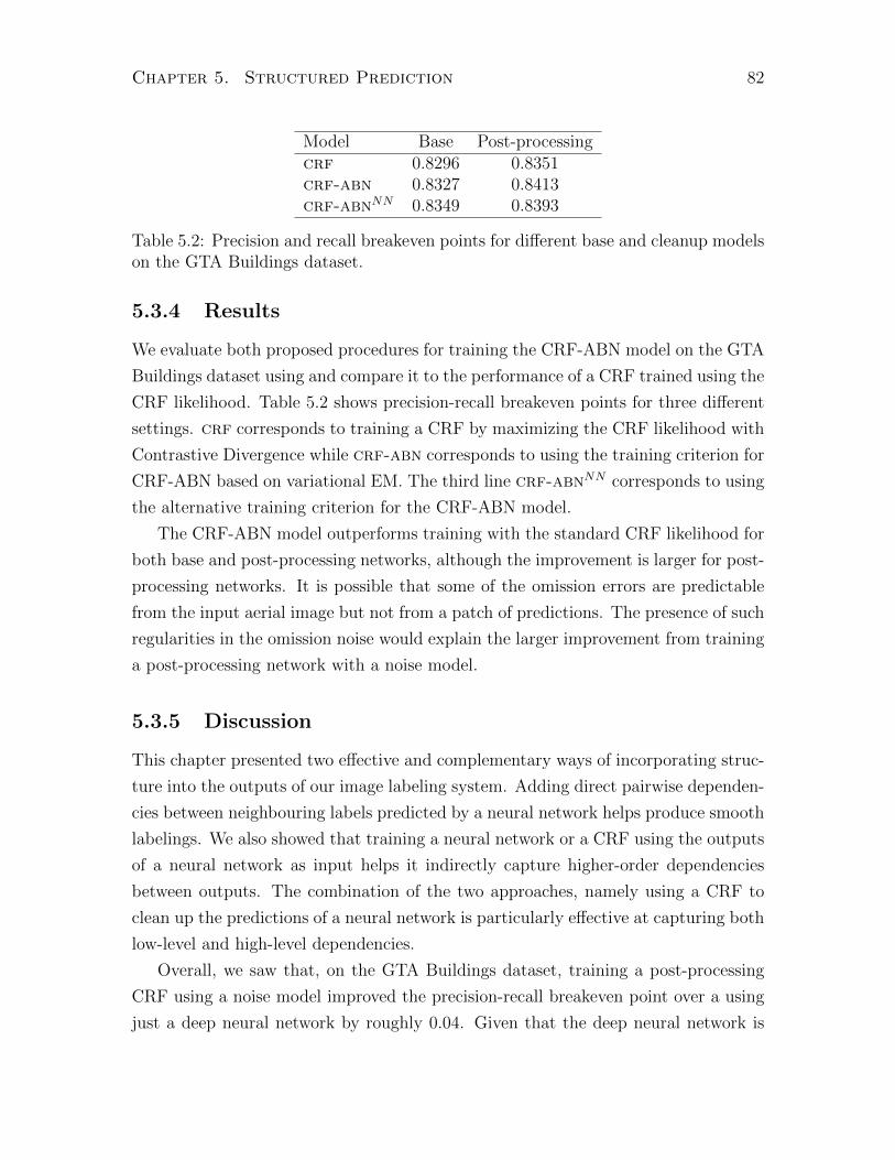
Chapter 5. Structured Prediction 82
Model Base Post-processingcrf 0.8296 0.8351crf-abn 0.8327 0.8413crf-abnNN 0.8349 0.8393
Table 5.2: Precision and recall breakeven points for different base and cleanup modelson the GTA Buildings dataset.
5.3.4 Results
We evaluate both proposed procedures for training the CRF-ABN model on the GTA
Buildings dataset using and compare it to the performance of a CRF trained using the
CRF likelihood. Table 5.2 shows precision-recall breakeven points for three different
settings. crf corresponds to training a CRF by maximizing the CRF likelihood with
Contrastive Divergence while crf-abn corresponds to using the training criterion for
CRF-ABN based on variational EM. The third line crf-abnNN corresponds to using
the alternative training criterion for the CRF-ABN model.
The CRF-ABN model outperforms training with the standard CRF likelihood for
both base and post-processing networks, although the improvement is larger for post-
processing networks. It is possible that some of the omission errors are predictable
from the input aerial image but not from a patch of predictions. The presence of such
regularities in the omission noise would explain the larger improvement from training
a post-processing network with a noise model.
5.3.5 Discussion
This chapter presented two effective and complementary ways of incorporating struc-
ture into the outputs of our image labeling system. Adding direct pairwise dependen-
cies between neighbouring labels predicted by a neural network helps produce smooth
labelings. We also showed that training a neural network or a CRF using the outputs
of a neural network as input helps it indirectly capture higher-order dependencies
between outputs. The combination of the two approaches, namely using a CRF to
clean up the predictions of a neural network is particularly effective at capturing both
low-level and high-level dependencies.
Overall, we saw that, on the GTA Buildings dataset, training a post-processing
CRF using a noise model improved the precision-recall breakeven point over a using
just a deep neural network by roughly 0.04. Given that the deep neural network is
Chapter 5. Structured Prediction 83
already a powerful model, the improvement is substantial.
There are a number of interesting extensions of the proposed models. One promis-
ing direction is to investigate the use of pairwise potentials that are modulated by
a neural network instead of a simple image-dependent term. Given that we found it
necessary to use image-dependent pairwise potentials in order to get an improvement
from using a CRF we believe that making this part of the model more powerful could
lead to substantial improvements. The promising results obtained on several image
labeling tasks in Jancsary et al. [2012] using a model where the pairwise potentials
are determined using regression trees provide further evidence.
Chapter 6
Large-Scale Evaluation
So far, we have presented a complete framework for learning to label aerial images, and
while we have provided experimental validation along the way, we have not directly
compared our results to the work of others. As we discussed in Chapter 2, the rarity
of direct comparisons between proposed aerial image interpretation methods is a long-
standing problem in the area and we believe that it is primarily caused by the lack
of high quality publicly available aerial image datasets. In this chapter, we introduce
the first large-scale and publicly available road and building detection datasets, and
evaluate the most promising methods from the rest of the thesis on the new datasets.
We hope that the availability of these new high-quality datasets will both facilitate
more comparisons of existing methods and lead to increased interest in aerial imagery
applications in the machine learning and computer vision communities. Furthermore,
the evaluation of methods presented in this thesis on challenging datasets that were
not used during the development of these methods offers further validation of their
effectiveness.
We have assembled three datasets using publicly available imagery and metadata.
Two of the datasets make use of imagery released by the state of Massachusetts 1
while the third dataset uses imagery released by the state of New York 2. All imagery
was rescaled to a resolution of 1 pixel per square meter. The target maps for all three
datasets were generated using data from the OpenStreetMap project. Target maps
for the test and validation portions of all three datasets were hand-corrected to make
1http://www.mass.gov/anf/research-and-tech/it-serv-and-support/application-serv/office-of-geographic-information-massgis/
2gis.ny.gov/gisdata/
84

Chapter 6. Large-Scale Evaluation 85
the evaluations more accurate.
6.1 Massachusetts Buildings Dataset
The Massachusetts Buildings Dataset consists of 151 aerial images of the Boston
area, with each of the images being 1500 × 1500 pixels for an area of 2.25 square
kilometers. Hence, the entire dataset covers roughly roughly 340 square kilometers.
We randomly split the data into a training set of 137 images, a test set of 10 images and
a validation set of 4 images. The target maps were obtained by rasterizing building
footprints obtained from the OpenStreetMap project. Unlike the GTA Buildings
dataset we have used throughout the thesis, this data was restricted to regions with
an average omission noise level of roughly 5% or less. It was possible to collect such
a large a mount of high quality building footprint data because the City of Boston
has contributed building footprints for the entire city to the OpenStreetMap project.
The dataset covers mostly urban and suburban areas and buildings of all sizes,
including individual houses and garages, are included in the labels. Figures 6.1(a)
and 6.1(b) show two representative regions from the Massachusetts Buildings dataset.
6.2 Massachusetts Roads Dataset
The Massachusetts Roads Dataset consists of 1171 aerial images of the state of Mas-
sachusetts. As with the building data, each image is 1500×1500 pixels in size, covering
an area of 2.25 square kilometers. We randomly split the data into a training set of
1108 images, a validation set of 14 images and a test set of 49 images. The dataset
covers a wide variety of urban, suburban, and rural regions and covers an area of over
2600 square kilometers. With the test set alone covering over 110 square kilometers,
this is by far the largest and most challenging aerial image labeling dataset. Fig-
ures 6.2(a) and 6.2(b) show two representative regions from the Massachusetts Roads
dataset.
The target maps were generated by rasterizing road centerlines obtained from
the OpenStreetMap project. We used a line thickness of 7 pixels and no smoothing
because, as we discovered in Chapter 4, using hard binary labels for training works
better than using soft binary labels.

Chapter 6. Large-Scale Evaluation 86
(a) (b)
(c) (d)
Figure 6.1: Figures 6.1(a) and 6.1(b) show two representative regions from the Mas-sachusetts Buildings dataset. Figures 6.1(c) and 6.1(d) show predictions of a post-processing network on these regions. Green pixels are true positives, red pixels arefalse positives, blue pixels are false negatives, and background pixels are true nega-tives.
6.3 Buffalo Roads Dataset
The Buffalo Roads dataset differs substantially from the other two datasets presented
in this chapter because it is primarily meant to be used as an additional test set for

Chapter 6. Large-Scale Evaluation 87
(a) (b)
(c) (d)
Figure 6.2: Figures 6.2(a) and 6.2(b) show two representative regions from the Mas-sachusetts Roads dataset. Figures 6.2(c) and 6.2(d) show predictions of a post-processing network on these regions.
the Massachusetts Roads dataset. Our aim was to construct a test set that was
collected in a different area and under different conditions from the Massachusetts
Roads dataset.
The dataset consists of 30 aerial images of the city of Buffalo with each image

Chapter 6. Large-Scale Evaluation 88
being 609 × 914 pixels at a resolution of one pixel per square meter. The dataset
was randomly split into a training set of 5 images, a validation set of 5 images and
a test set of 20 images. Since the training set is so small it is unlikely that it can be
used to learn a good road detector and hence it is mostly available for the purposes
of adapting models trained on the Massachusetts data to the Buffalo dataset. As
with the Massachusetts Roads dataset, the target maps were generated by rasterizing
road centerlines obtained from the OpenStreetMap project with a line thickness of 7
pixels.
The dataset includes a wide variety of roads from both urban and suburban areas,
including significant amounts of occlusion from trees. Figures 6.3(a) and 6.3(b) show
two representative regions from the Buffalo Roads dataset. The conditions under
which the Buffalo Roads dataset was collected are clearly significantly different from
those of the Massachusetts Roads dataset, suggesting that training a model on the
later while evaluating it on the former may be a challenging task.
6.4 Results
6.4.1 Massachusetts Datasets
The main model we evaluated on the Massachusetts datasets is a large convolutional
neural network. The input to the model is a 64 by 64 aerial image patch. The first
hidden layer is a convolution layer with 64 16× 16 filters with stride 4. It is followed
by 2 × 2 max pooling with stride 1. The second hidden layer is also convolutional
with 112 filters of size 4×4 with stride 1, followed by a third convolutional layer with
80 filters of size 3 × 3 with stride 1. The fourth, and final, hidden layer is a fully
connected layer with 4096 hidden units. All four hidden layers consist of rectified
linear units. As before, the output layer is a fully-connected layer of 256 logistic
units.
The neural network was trained using stochastic gradient descent with minibatches
of size 128 using the hyper-parameter values described in Chapter 3. Additionally,
after every 220 training cases, we multiplied the learning rate by 0.95. Training
stopped after 225 cases had been processed.
We evaluated two other methods in addition to the plain neural network – a CRF
initialized with the neural network weights, and a post-processing network trained
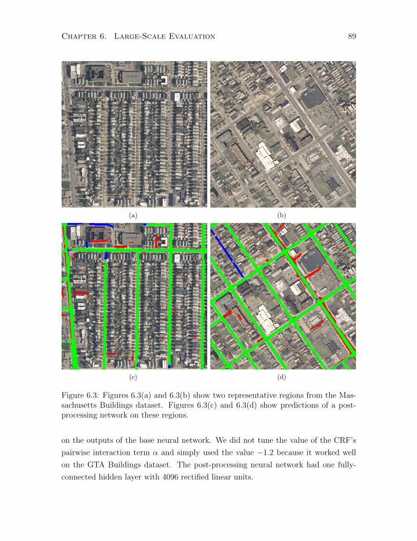
Chapter 6. Large-Scale Evaluation 89
(a) (b)
(c) (d)
Figure 6.3: Figures 6.3(a) and 6.3(b) show two representative regions from the Mas-sachusetts Buildings dataset. Figures 6.3(c) and 6.3(d) show predictions of a post-processing network on these regions.
on the outputs of the base neural network. We did not tune the value of the CRF’s
pairwise interaction term α and simply used the value −1.2 because it worked well
on the GTA Buildings dataset. The post-processing neural network had one fully-
connected hidden layer with 4096 rectified linear units.

Chapter 6. Large-Scale Evaluation 90
ModelDataset
Mass. Roads Mass. BuildingsNeural net 0.8873 0.9150CRF 0.8904 0.9211Post-processing net 0.9006 0.9203
Table 6.1: Precision-recall breakeven points for different models on the Massachusettsdatasets.
Table 6.1 shows the precision-recall breakeven points on the Massachusetts datasets
for the three models described above. We see that there is a relatively small improve-
ment from using a CRF on both datasets and that post-processing neural networks
outperform CRFs on road data. It is surprising that the improvement obtained by
structured models on the building data is quite small compared to the improvement
obtained on the GTA Buildings dataset. The main difference between the datasets
is that the Massachusetts Buildings dataset is dominated by individual houses while
the GTA Buildings dataset consists almost entirely of larger buildings. It is possible
that the gain from structured prediction on the Massachusetts data is smaller because
structure is not as important for detecting small objects such as houses.
To get a better idea of how well these models work, we include visualizations of
predictions of the post-processing networks on test data from both datasets. Fig-
ures 6.1(c) and 6.1(d) show predictions of the post-processing neural network trained
on the building data for the regions shown in Figures 6.1(a) and 6.1(b). The network
is very good at detecting individual houses but does less well on larger buildings.
This is not entirely surprising because there is significantly more variation in the
appearance of large buildings and the model saw fewer of them during training Fig-
ures 6.2(c) and 6.2(d) show predictions of the post-processing neural network trained
on the Massachusetts Roads dataset. As these results show, the model is very good
at detecting roads in a variety of settings and even under significant occlusions by
trees.
6.4.2 Buffalo Roads Dataset
The Buffalo Roads dataset was constructed in order to evaluate how well models
trained on the Massachusetts Roads dataset generalize to substantially different con-
ditions. Table 6.2 shows the precision-recall breakeven points for a number of different
Chapter 6. Large-Scale Evaluation 91
models on the Buffalo Roads test set. NN Mass corresponds to the big convolutional
neural network trained on the Massachusetts data and this model clearly works poorly
on the Buffalo data. NN Buffalo corresponds to the same convolutional architecture,
but trained on the small Buffalo Roads training set. While this model works surpris-
ingly well given that it was trained on less than 3 square kilometers of imagery, it
still achieves a breakeven point of just 0.7960.
Comparing images from the Massachusetts (Figures 6.2(a) and 6.2(b)) and Buffalo
(Figures 6.3(a) and6.3(b)) datasets suggests that the main difference may be in the
distribution of colours and that the structure of the roads may be largely the same.
Using this hypothesis as motivation we evaluated several ways of adapting the network
trained on Massachusetts data to Buffalo data using the small training set.
One straightforward way of compensating for the difference in colour distribution
between the datasets is by transforming the Buffalo data to have the same colour
histogram as the Massachusetts data. The third model from Table 6.2 corresponds to
running the NN Mass model on colour corrected Buffalo data. This simple strategy
requires only unlabeled data and turns out to be reasonably effective, as it boosts
the breakeven-point from 0.5613 to 0.8099. The other strategy for adapting the NN
Mass model to the Buffalo data involves using the small training set to finetune the
weights of the model. We started with the weights of NN Mass, trained it on the
Buffalo Roads training set for 128 epochs using a learning rate of 10−4, and saved the
weights that gave the highest log likelihood on the Buffalo Roads validation set. Using
the training set to finetune the weights in this manner improved the breakeven point
of the NN Mass model to 0.8785. While this number is comparable to the breakeven
point of the NN Mass model on the Massachusetts test set it does not mean that
the model works equally well on Buffalo data. In fact, we find that the Buffalo test
set appears to be easier than the Massachusetts test set, explaining the comparable
performance. Nevertheless, these results show that a model trained under one set of
conditions can be adapted to a new dataset using a small amount of labeled training
data.
The last model we evaluated on the Buffalo dataset is a post-processing neural
network trained on Massachusetts. We applied it to the outputs of the finetuned NN
Mass model and achieved a breakeven point of 0.8918 on the Buffalo test set. This
shows that post-processing networks do not necessarily have to be retrained for each
new dataset as long as the target object class is the same. Figures 6.3(c) and 6.3(d)

Chapter 6. Large-Scale Evaluation 92
Model Breakeven pointNN Mass. 0.5613NN Buffalo 0.7960NN Mass. + histogram matching 0.8099NN Mass. + finetuning 0.8785NN Mass. + finetuning + post-processing 0.8918
Table 6.2: Precision-recall values on the Buffalo Roads test.
show the predictions of this-post processing network on parts of the Buffalo Roads
test set.
Chapter 7
Conclusions and Future Work
This thesis presented a complete framework for learning to label aerial imagery, ad-
vancing the state of the art in both the difficulty of the tasks considered and the
quality of the predictions. Our framework addressed what we see as the three central
issues in learning from aerial imagery – learning of discriminative features, learning
from noisy data, and doing structured prediction.
In Chapter 3, we showed that neural networks trained on large amounts of la-
beled images using modern GPUs produced good performance on challenging real
world road and building detection datasets. We also showed that deep neural net-
works produced much more accurate predictions than shallow networks. In particular,
we found that deep convolutional neural networks with small amounts of maximum
pooling were particularly effective on aerial image labeling tasks.
Our introduction of noise models for dealing with omission and registration noise
in Chapter 4 is, to the best of our knowledge, the first attempt to address the problem
of noisy labels in aerial imagery. It is also, along with the work of Jain [Jain et al.,
2010] the first work to directly address the issue of noise in pixel labeling tasks. While
our ABN and TABN noise models introduce some level of robustness to two types of
label noise, we also looked at how noise in the training data affects a system trained on
this data. By using synthetic omission noise, we found that, somewhat surprisingly,
a neural network trained on a road detection dataset with as much as 40% of the
road labels deleted still performed quite well. Hence, label noise has a negative but
relatively small effect on neural networks.
Chapter 5 showed that the quality of the predictions can be further improved
using two complementary ways of incorporating structure into the predictions of our
93

Chapter 7. Conclusions and Future Work 94
system. Post-processing neural networks learn to improve the predictions of a base
predictor using our patch-framework from Chapter 3. By reusing the existing frame-
work, post-processing neural networks are able to handle massive datasets using our
GPU-based implementation and are capable of learning complex features of the in-
put predictions. We also showed that adding direct, image-dependent dependencies
between the outputs of a neural network, turning it into a CRF, improves the predic-
tions by encouraging smoothness between neighbouring labels, a property of the data
that is not easily learned by post-processing neural networks. While training such
models can be troublesome, we showed that most of the benefit can be obtained by
training the neural network separately before using its weights to initialize a CRF.
Finally, we introduced the first large-scale publicly available datasets for both road
and building detection along with benchmarks that others can compare to. In both
datasets, the regions used for testing are both much larger and more varied than any
aerial image labeling dataset, both public or private, that we are aware of. We believe
that the availability of large and realistic datasets for aerial image labeling has the
potential to significantly advance the area. In particular, we hope that these datasets
will stimulate interest among computer vision and machine learning researchers.
While there are many possible directions for improving our system, it is important
to consider which ones will lead to the biggest gain in the quality of predictions.
Despite the significant gains obtained by incorporating structured prediction into our
system in Chapter 5, it is clear that neural network design choices such as using
several layers instead of one and convolutions instead of locally connected units lead
to the biggest gains in our thesis. For this reason we believe that putting more effort
into finding a good neural network architecture is likely to lead to further significant
gains. As we mentioned earlier, one way of improving the architecture is by doing a
better hyper-parameter search using Bayesian optimization techniques [Snoek et al.,
2012]. The recently introduced stochastic pooling [Zeiler and Fergus, 2013] has been
shown to work much better than the max pooling operation we use and should be
explored within our system.
In addition to finding a good neural network architecture, it is also important
to have a good procedure for fitting it to the data. While we have shown that
stochastic gradient descent on the negative log likelihood works well, we believe that
exploring better loss functions is likely to lead to big improvements in the predictions.
For example, the area under the precision-recall curve is a better measure of the
Chapter 7. Conclusions and Future Work 95
quality of the predictions for road and building detection than log likelihood, hence
directly maximizing the area under the curve is almost certainly a better approach.
Furthermore, due to the fact that even our largest models do not seem to suffer from
serious overfitting problems, we believe that exploring better optimization methods
is a promising direction.
Beyond improving the architecture and training procedure of the neural network,
improving the structured prediction aspect of the model is also likely to lead to
significant improvements. The fully connected CRF model recently introduced by
Krahenbuhl and Koltun [2011] has significantly improved the state-of-the-art in image
labeling and is likely to work well on aerial imagery. One interesting question relating
to these types of models is whether their performance could be improved by jointly
training all parameters using the model likelihood. We had limited success with
finetuning the unary potentials of our CRFs using the CRF likelihood, which could
simply be the result of using a poor approximate learning procedure. Still, we believe
that an end-to-end training procedure is preferable to one in which components are
learned separately.
Another important aspect of the overall system design is what data it is trained
on, which is equivalent to an underlying assumption about what type of data the
system is expected to work on. We have focused on improving performance on several
large and realistic aerial image labeling datasets, the most diverse of which covered
different parts of the state of Massachusetts. Our success on such datasets suggests
that given enough aerial imagery of a geographic area of limited size it is possible
to learn a good road or building detector for this area. Ultimately, the goal of the
field is probably to build a system that works well for imagery taken from any part
of the world under any reasonable conditions. While we showed some success with
training on one region while testing on another one and with adapting an existing
system to a new region using a small amount of labeled data, building a single good
detector probably requires even more varied datasets that cover all distinct regions
of the world. Unfortunately, at this point, freely available high resolution imagery is
generally limited to parts of Europe and North America.
Furthermore, being able to label pixels of an aerial image with semantic classes is
not the ultimate goal of aerial image interpretation but merely a useful abstraction
of the underlying problems. To make our system truly useful it must be incorporated
into a Geographic Information System (GIS). Two possible use cases for a pixel label-
Chapter 7. Conclusions and Future Work 96
ing system in a GIS environment are map updating and automatic object extraction.
In the case of map updating, an existing, possibly outdated map needs to be updated
based on recent aerial imagery. While maps are usually stored in vector form and
our system produces raster images as its predictions, comparing a vector map and a
raster predicted map should be relatively straightforward. By looking for parts of the
predicted map that significantly disagree with the reference vector map, our system
could be used to automatically find regions that need updating. We believe that the
quality of the predictions of our system on the Massachusetts Roads data is already
sufficient to make it useful in an updating setting.
Finally, we believe that our system could also be used to facilitate automatic ex-
traction of objects from aerial imagery. In the case of roads, this requires extracting
vector representations of road centerlines from predicted raster maps. We have ex-
perimented with the automatic line extraction algorithm of Steger [1998] and found
that it works well when applied to predicted road maps produced by our system. It is
interesting that this algorithm was originally applied to extracting roads directly from
aerial imagery, but it works substantially better when applied to the output of our
system. This suggests that previous work on finding roads by applying active contour
models directly to aerial images can be revisited using our predicted maps as input.
The combination of strong topological constraints enforced by such models with a
data association potential produced by our system could be especially powerful. In
the case of buildings, we can already extract their locations by finding the centres
of mass of connected components of predicted building pixels. Extracting complete
building footprints would likely require training on even higher resolution input data,
but could probably be done using existing polygon extraction algorithms. Again, we
see the possibility of using the outputs of our system as a powerful data association
term in existing building detection methods that use strong topological constraints.

Bibliography
Ruzena Bajcsy and Mohamad Tavakoli. Computer recognition of roads from satellite
pictures. IEEE Transactions on Systems, Man, and Cybernetics, 6(9):623–637,
September 1976.
E. P. Baltsavias. Object extraction and revision by image analysis using existing
geodata and knowledge: current status and steps towards operational systems.
ISPRS Journal of Photogrammetry and Remote Sensing, 58(3-4):129–151, January
2004.
Jon A Benediktsson, Philip H Swain, and Okan K Ersoy. Neural network approaches
versus statistical methods in classification of multisource remote sensing data. IEEE
Transactions on Geoscience and Remote Sensing, 28(4):540–552, 1990.
James S. Bergstra, Rmi Bardenet, Yoshua Bengio, and Balzs Kgl. Algorithms for
hyper-parameter optimization. In J. Shawe-Taylor, R.S. Zemel, P. Bartlett, F.C.N.
Pereira, and K.Q. Weinberger, editors, Advances in Neural Information Processing
Systems 24, pages 2546–2554. 2011.
H. Bischof, W. Schneider, and A. J. Pinz. Multispectral classification of landsat im-
ages using neural networks. IEEE Transaction on Geoscience and Remote Sensing,
30(3):482–490, 1993.
Christopher M. Bishop. Pattern Recognition and Machine Learning. Springer-Verlag
New York, Inc., Secaucus, NJ, USA, 2006. ISBN 0387310738.
Julian E. Boggess. Identification of roads in satellite imagery using artificial neural
networks: A contextual approach. Technical report, Mississippi State University,
1993.
97

BIBLIOGRAPHY 98
L. Bruzzone and D.F. Prieto. Automatic analysis of the difference image for unsuper-
vised change detection. Geoscience and Remote Sensing, IEEE Transactions on,
38(3):1171–1182, 2000.
Adam Coates, Andrew Y. Ng, and Honglak Lee. An analysis of single-layer net-
works in unsupervised feature learning. Journal of Machine Learning Research -
Proceedings Track, 15:215–223, 2011.
George E. Dahl, Marc’Aurelio Ranzato, Abdel-rahman Mohamed, and Geoffrey E.
Hinton. Phone recognition with the mean-covariance restricted Boltzmann ma-
chine. In J. Lafferty, C. K. I. Williams, J. Shawe-Taylor, R.S. Zemel, and A. Cu-
lotta, editors, Advances in Neural Information Processing Systems 23, pages 469–
477. 2010.
S.E. Decatur. Application of neural networks to terrain classification. In International
Joint Conference on Neural Networks, volume 1, pages 283–288, June 1989.
Piotr Dollar, Zhuowen Tu, and Serge Belongie. Supervised learning of edges and
object boundaries. In Proceedings of the 2006 IEEE Computer Society Conference
on Computer Vision and Pattern Recognition, pages 1964–1971, 2006.
C. Farabet, C. Couprie, L. Najman, and Y. LeCun. Scene parsing with multiscale
feature learning, purity trees, and optimal covers. arXiv preprint arXiv:1202.2160,
2012.
S. Gould, J. Rodgers, D. Cohen, G. Elidan, and D. Koller. Multi-class segmentation
with relative location prior. International Journal of Computer Vision, 80(3):300–
316, 2008.
D. M. Greig, B. T. Porteous, and A. H. Seheult. Exact maximum a posteriori estima-
tion for binary images. Journal of the Royal Statistical Society. Series B (Method-
ological), 51(2):271–279, 1989.
R. Haralick. Automatic remote sensor image processing. Digital Picture Analysis,
pages 5–63, 1976.
Robert M. Haralick, K. Shanmugam, and Its’Hak Dinstein. Textural Features for
Image Classification. IEEE Transactions on Systems, Man, and Cybernetics, 3(6):
610–621, November 1973.

BIBLIOGRAPHY 99
Xuming He, Richard S. Zemel, and Miguel A. Carreira-Perpinan. Multiscale condi-
tional random fields for image labeling. In CVPR ’04: Proceedings of the 2004
IEEE Computer Society Conference on Computer Vision and Pattern Recognition,
pages 695–702, 2004.
Xuming He, R Zemel, and Deb Ray. Learning and incorporating top-down cues in
image segmentation. In European Conference on Computer Vision, 2006.
Geoffrey Hinton. Training products of experts by minimizing contrastive divergence.
Neural Computation, 14(8):1771–1800, 2002.
C. Huang, L. S. Davis, and J. R. G. Townshend. An assessment of support vector
machines for land cover classification. International Journal of Remote Sensing, 23
(4):725–749, 2002.
Xin Huang and Liangpei Zhang. Road centreline extraction from high-resolution
imagery based on multiscale structural features and support vector machines. In-
ternational Journal of Remote Sensing, 30(8):1977–1987, 2009.
J. M. Idelsohn. A learning system for terrain recognition. Pattern Recognition, 2(4):
293–296, 1970.
Viren Jain, Benjamin Bollmann, Mark Richardson, Daniel R. Berger, Moritz Helm-
staedter, Kevin L. Briggman, Winfried Denk, Jared B. Bowden, John M. Menden-
hall, Wickliffe C. Abraham, Kristen M. Harris, N. Kasthuri, Ken J. Hayworth,
Richard Schalek, Juan Carlos Tapia, Jeff W. Lichtman, and H. Sebastian Seung.
Boundary learning by optimization with topological constraints. In The Twenty-
Third IEEE Conference on Computer Vision and Pattern Recognition, pages 2488–
2495. IEEE, 2010. doi: http://dx.doi.org/10.1109/CVPR.2010.5539950.
Jeremy Jancsary, Sebastian Nowozin, Toby Sharp, and Carsten Rother. Regression
tree fields - an efficient, non-parametric approach to image labeling problems. In
CVPR, pages 2376–2383, 2012.
Kevin Jarrett, Koray Kavukcuoglu, Marc’Aurelio Ranzato, and Yann LeCun. What
is the best multi-stage architecture for object recognition? In Proc. International
Conference on Computer Vision (ICCV’09). IEEE, 2009.

BIBLIOGRAPHY 100
David M. McKeown Jr., Wilson A. Harvey, and John P. McDermott. Rule-based
interpretation of aerial imagery. IEEE Trans. Pattern Anal. Mach. Intell., 7(5):
570–585, 1985.
R. L. Kettig and D. A. Landgrebe. Classification of multispectral image data by
extraction and classification of homogeneous objects. IEEE Transactions on Geo-
science Electronics, 14:19–26, 1976.
Stefan Kluckner and Horst Bischof. Semantic classification by covariance descriptors
within a randomized forest. In Computer Vision Workshops (ICCV), pages 665–
672. IEEE, 2009.
Stefan Kluckner, Thomas Mauthner, Peter M. Roth, and Horst Bischof. Semantic
classification in aerial imagery by integrating appearance and height information.
In ACCV, volume 5995 of Lecture Notes in Computer Science, pages 477–488.
Springer, 2009.
Pushmeet Kohli, Lubor Ladicky, and Philip H. S. Torr. Robust Higher Order Poten-
tials for Enforcing Label Consistency. International Journal of Computer Vision,
82(3):302–324, January 2009.
Philipp Krahenbuhl and Vladlen Koltun. Efficient inference in fully connected crfs
with gaussian edge potentials. In J. Shawe-Taylor, R.S. Zemel, P. Bartlett, F.C.N.
Pereira, and K.Q. Weinberger, editors, Advances in Neural Information Processing
Systems 24, pages 109–117. 2011.
Alex Krizhevsky. Convolutional deep belief networks on cifar-10. Technical report,
University of Toronto, 2011.
S. Lazebnik, C. Schmid, and J. Ponce. Beyond Bags of Features: Spatial Pyramid
Matching for Recognizing Natural Scene Categories. Computer Vision and Pattern
Recognition, 2:2169–2178, 2006.
Y LeCun, FJ Huang, and Leon Bottou. Learning methods for generic object recogni-
tion with invariance to pose and lighting. In Computer Vision and Pattern Recog-
nition, 2004.
BIBLIOGRAPHY 101
Jonathan Lee, Ronald C. Weger, Sailes K. Sengupta, and Ronald M. Welch. A Neural
Network Approach to Cloud Classification. IEEE Transactions on Geoscience and
Remote Sensing, 28:846–855, September 1990.
Helmut Mayer. Object extraction in photogrammetric computer vision. ISPRS Jour-
nal of Photogrammetry and Remote Sensing, 63(2):213–222, March 2008.
Volodymyr Mnih and Geoffrey Hinton. Learning to detect roads in high-resolution
aerial images. In Proceedings of the 11th European Conference on Computer Vision
(ECCV), September 2010.
Volodymyr Mnih and Geoffrey Hinton. Learning to label aerial images from noisy
data. In Andrew McCallum and Sam Roweis, editors, Proceedings of the 29th
Annual International Conference on Machine Learning (ICML 2012), June 2012.
Volodymyr Mnih, Hugo Larochelle, and Geoffrey Hinton. Conditional restricted boltz-
mann machines for structured output prediction. In Proceedings of the International
Conference on Uncertainty in Artificial Intelligence, 2011.
J.W. Modestino and J. Zhang. A Markov random field model-based approach to image
interpretation. In Computer Vision and Pattern Recognition, 1989. Proceedings
CVPR’89., IEEE Computer Society Conference on, pages 458–465. IEEE, 1989.
Vinod Nair and Geoffrey E. Hinton. Rectified linear units improve restricted boltz-
mann machines. In ICML, pages 807–814, 2010.
T. Nguyen, Stefan Kluckner, Horst Bischof, and Franz Leberl. Aerial Photo Build-
ing Classification by Stacking Appearance and Elevation Measurements. In In:
Proceedings ISPRS, 100 Years ISPRS-Advancing Remote Sensing Science, on CD-
ROM, 2010.
Thuy Thi Nguyen, Helmut Grabner, Horst Bischof, and Barbara Gruber. On-line
Boosting for Car Detection from Aerial Images. In 2007 IEEE International Con-
ference on Research, Innovation and Vision for the Future, pages 87–95. IEEE,
March 2007.
J Niemeyer, C. Mallet, F Rottensteiner, and U Sorgel. Conditional Random Fields
for the Classification of LiDAR Point Clouds. International Archives of Photogram-
metry and Remote Sensing, 38:4, 2008.
BIBLIOGRAPHY 102
J.D. Paola and R.A. Schowengerdt. A detailed comparison of backpropagation neu-
ral network and maximum-likelihood classifiers for urban land use classification.
Geoscience and Remote Sensing, IEEE Transactions on, 33(4):981–996, jul 1995.
Jake Porway, Kristy Wang, Benjamin Yao, and Song Chun Zhu. A hierarchical and
contextual model for aerial image understanding. In Computer Vision and Pattern
Recognition, IEEE Computer Society Conference on, 2008.
Roberto Rigamonti, Engin Turetken, German Gonzalez, and Pascal Fua. Filter Learn-
ing for Linear Structure. Technical report, Swiss Federal Institute of Technology,
Lausanne (EPFL), 2011.
Pierre Sermanet, Soumith Chintala, and Yann LeCun. Convolutional neural net-
works applied to house numbers digit classification. In Proceedings of International
Conference on Pattern Recognition (ICPR’12), 2012.
Jamie Shotton, Matthew Johnson, and R. Cipolla. Semantic texton forests for image
categorization and segmentation. In Computer Vision and Pattern Recognition,
2008. IEEE Conference on, pages 1–8. IEEE, 2008.
Jasper Snoek, Hugo Larochelle, and Ryan Prescott Adams. Practical bayesian op-
timization of machine learning algorithms. In Neural Information Processing Sys-
tems, 2012.
Xiaomu Song, Guoliang Fan, and Mahesh Rao. Automatic CRP Mapping Using
Machine Learning Approaches. IEEE Transactions on Geoscience and Remote
Sensing, 43(4):888–897, 2005.
Carsten Steger. An unbiased detector of curvilinear structures. Pattern Analysis
and Machine Intelligence, IEEE Transactions on, 20(2):113 –125, feb 1998. ISSN
0162-8828. doi: 10.1109/34.659930.
R.H. Swendsen and J.S. Wang. Nonuniversal critical dynamics in monte carlo simu-
lations. Physical Review Letters, 58(2):86, 1987.
Srinivas Turaga, Kevin Briggman, Moritz Helmstaedter, Winfried Denk, and Se-
bastian Seung. Maximin affinity learning of image segmentation. In Y. Bengio,
D. Schuurmans, J. Lafferty, C. K. I. Williams, and A. Culotta, editors, Advances
in Neural Information Processing Systems 22, pages 1865–1873. 2009.
BIBLIOGRAPHY 103
P. Viola and M. Jones. Rapid object detection using a boosted cascade of simple
features. In Computer Vision and Pattern Recognition, 2001. CVPR 2001. Pro-
ceedings of the 2001 IEEE Computer Society Conference on, volume 1, pages I–511.
IEEE, 2001.
Christian Wiedemann, Christian Heipke, Helmut Mayer, and Olivier Jamet. Em-
pirical evaluation of automatically extracted road axes. In Empirical Evaluation
Techniques in Computer Vision, pages 172–187, 1998.
M. D. Zeiler and R. Fergus. Stochastic Pooling for Regularization of Deep Convolu-
tional Neural Networks. ArXiv e-prints, January 2013.
Ping Zhong and Runsheng Wang. Using combination of statistical models and multi-
level structural information for detecting urban areas from a single gray-level image.
Geoscience and Remote Sensing, IEEE Transactions on, 45(5):1469–1482, 2007.