by pasu“loharjun0 - vtechworks.lib.vt.edu · generated by corelap. dedication this work is...

7M

\ /A DECISION THEORETIC APPROACH TO THE GENERAL LAYOUT PROBLEM

by

Pasu“Loharjun0

Dissertation submitted to the Faculty of the

Virginia Polytechnic Institute and State University

in partial fulfillment of the requirements for the degree of

Doctor of Philosophy

in

Industrial Engineering and Operations Research

APPROVED:

Subhash C. Sarin, Chairman

Marvin H. Egee Wolter J. Fabäyckyl

{ '‘

Charles J. yaääborg " (Ma;2lyn Sijäones

March, 1986

Blacksburg, Virginia

A DECISION THEORETIC APPROACH TO THE GENERAL LAYOUT PROBLEMä by

Pasu Loharjun

§_ Subhash C. Sarin, ChairmanFX

Industrial Engineering and Operations Research

(ABSTRACT)

This research is devoted to the development of a multiobjec-

tive facility layout creation methodology. This methodology

seeks to extend the scope of existing computerized and manual

layout creation methods by capturing a greater level of both

intuitive and quantitative inputs in a method applicable for

moderate to large-scale problems. To do this, an extended

theoretical basis for decision theoretic models applicable

to layout design is described„ Using these models as an

evaluation basis, a new optimizing layout creation strategy

is developed and a decision support system for its implemen-

tation is presented. The new layout creation method is com-

putationally attractive, and based on extensive computational

experience, is foumd to give better solutions than those

generated by CORELAP.

DEDICATION

This work is dedicated to my Grandfathers,

to whom education was always so important.

I think they would have been proud.

Dedication

ACKNOWLEDGEMENTS

The completion of a Ph.D. dissertation has been a monumental

goal in my life. There are many people without whom I would

not have been able to reach this goal.

I would like to thank all the members of my advisory commit-

tee for their valuable assistance throughout the various

stages of this research. I wish to especially thank Dr.

Charles J. Malmborg for introducing me to this research topic

and giving useful insight during the early phase of this re-

search. I would also like to thank Dr. Marvin H. Agee for

his constructive comments.

Foremost, I would like to thank Dr. Subhash C. Sarin, my

chairman, for his valuable guidance, suggestions, insight and

timely encouragement in carrying out this research and pre-

paring the final draft.

I would also like to thank Drs. Wolter J.Fabrycky and Robert

D. Dryden for awarding me Graduate Teaching Assistantships

during 1983-1985.

A special and personal regards to my parents for their love

and continuous support during my education at Virginia Tech.

Acknowledgements iv

TABLE OF CONTENTS

1. INTRODUCTION ................... 1

1.1 Statement of Problem ............... 1

1.2 Objectives of the Research ............ 3

1.3 Organization of the Dissertation ......... 4

2. LITERATURE REVIEW ................. 6

2.1 Review of Literature on Facility Layout Design Ap-

W proaches ...................... 6

2.1.1 Computerized Approaches l........... 10

2.1.2 Multicriteria Approaches . . ......... 35

2.1.3 Graph Theoretic Approaches .......... 38

2.1.4 Mathematical Modeling Approaches ....... 39

2.1.5 Summary and Conclusion ............ 44

2.2 Literature Review of Decision Theory ....... 45

2.2.1 Multiattribute Value Theory ......... 46

2.2.2 Measurable Multiattribute Value Functions . . 52

2.2.3 Multiattribute Value Function: A Binary Case . 54

2.2.4 Summary and Conclusion ............ 56

V3. DECISION THEORETIC APPROACHES TO THE GENERAL PLANT

LAYOUT PROBLEM ................... 58

3.1 Introduction ................... 58

3.1.1 Statement of Need for the Alternative Approach 58

Table of Contents v

3.1.2 Objectives of the Alternative Approach .... 59

3.1.3 Overview of the Chapter ........... 61

3.2 Measurement Considerations ............ 61

3.2.1 The Multiattribute Nature of the Facility Layout

Problem ...................... 62

3.2.2 The Need to Consider the Mixed Continuous and

Discrete Multiattribute Problem .......... 63

3.2.3 The Insufficiency of Present Axiomatic Systems 64

3.2.4 An Axiomatic System for the Mixed Case .... 68

3.2.5 Summary and Conclusion ............ 69”

3.3 Application of Decision Theory to the Layout Design

Problem ....................... 69

3.3.1 Extension of the REL Construct to Incorporate

Multiattribute Value Functions .......... 71

3.3.1.1 Efficient Assessment of the Value Functions 73l

3.3.1.2 Overview of Assessment Software ..... 74

3.3.2 Utilization of the Multiattribute Value Functions

in Layout Creation ................ 75

3.3.2.1 Description of the Procedure ....... 75

3.3.2.2 Advantages Over Existing Methods ..... 76

3.3.3 Overall Multiattribute Evaluation of Layout Al-,

ternatives .·................... 76

3.4 The Main Steps of the Proposed Procedure for layout

Design ....................... 77

3.5 Summary and Conclusions ............. 83

Table of Contents vi

4. A DECISION SUPPORT SYSTEM FOR FACILITY LAYOUT . . . 84

4.1 The Man Machine Concept of Decision Making Applied

to Facility Layout ................. 85

4.1.1 Description of Comparative Advantages .... 85

4.1.2 Overview of the Decision Support System . . . 86

4.2 Description of the Decision Support System .... 87

p 4.2.1 Data Requirements .............. 87

4.2.2 User Interaction ............... 89

4.2.3 Assumptions of the Modeling Approach ..... 89

4.2.4 Interfacing the Modules of the System .... 9O

4.2.5 Advantages of the System ........... 91

4.3 Summary and Conclusions ............. 92

5. AXIOMATIC BASIS FOR MIXED ATTRIBUTE CASES ..... 93

5.1 Notations and basic definitions ......... 94

5.1.1 Alternative space .............. 94

5.1.2 Weak ordering ................ 94

5.1.3 Essentialism ................. 95

5.1.4 Archimedean property ............. 95

5.1.5 Double cancellation ............. 96

5.1.6 Solvability ................. 96

5.2 Mixed additive case using compensatory independence 96

5.2.1 Definitions of independence conditions .... 97

5.2.1.1 Preferential independence ........ 97

5.2.1.2 Mutual preferential independence ..... 97

5.2.1.3 Compensatory independence ........ 98

Table of Contents vii

5.2.2 Theorem ................... 98

5.2.3 Proof .................... 99

5.3 Mixed additive case using Epsilon solvability . 102

5.3.1 Definition of epsilon solvability ..... 102

5.3.2 Theorem . . Q ............... 104

5.3.3 Proof ................... 105

5.4 Mixed multilinear case ............. 108

5.4.1 Theorem .................. 108

5.4.2 Proof ................... 109

5.5 Mixed multiplicative case ........... 112

5.5.1 Theorem .................. 112

5.5.2 Proof ................... 113

516 Mixed additive interdependent case ....... 115

. 5.6.1 Theorem .............A..... 115

5.6.2 Proof ................... 117

5.7 Summary and Conclusion ............. 120

6. METHODOLOGY FOR CREATING LAYOUT ALTERNATIVES . . 121

6.1 Layout design as a quadratic assignment problem 122

6.2 Literature Review of Procedures to Solve the QAP 124

6.2.1 Exact methods employing Branch and Bound . . 125

6.2.2 Exact methods not employing Branch and Bound 131

6.2.3 Heuristic Methods ............. 136

6.3 A Solution procedure for the determination of the

initial layout ..................· 142

6.4 A procedure for determining the Final Layout . . 151

Table of Contents viii

6.5 The overall layout design procedure ...... 153

6.6 An Example Problem ............... 155

6.6.1 Description of the Example Problem ..... 155

6.6.2 Layouts obtained using CORELAP and ALDEP . . 157

6.6.3 Results of experimentation with the proposed ·„

procedure .................... 167

6.7 Summary and conclusion ............. 184

7. SUMMARY, CONCLUSION, AND RECOMMENDATIONS .... 185

7.1 Summary and Conclusion ............. 186

7.1.1 A decision theoretic approach to layout design 186

7.1.2 Justification of the decision theoretic approach 187

7.1.3 Solution procedures for the quadratic assignment

problem ..................... 188

7.1.4 Decision support system for the layout design

problem ..................... 189

7.1.5 Results of Experimentation ......... 191

7.2 Recommendation ................. 191

BIBLIOGRAPHY .................... 193

APPENDIX A. DESCRIPTION.OF PROGRAMS IN THE DECISION

SUPPORT SYSTEM .................. 199

APPENDIX B. A COMPUTER RUN OF THE EXAMPLE PROBLEM . 203

Table of Contents ix

APPENDIX C. RANDOM MATRIX GENERATOR ........ 246

VITA ........................ 247

Table of Contents ' lx

LIST OF ILLUSTRATIONS

Figure 1.1 Principle categories of factors forfor consideration in facility design .... 2

Figure 2.1 Layout example problem .......... 12

Figure 2.2 Flow chart of CRAFT ............ 14

Figure 2.3 CRAFT's creation process ......... 15

Figure 2.4 Flow chart of PLANET ........... 19

Figure 2.5 PLANET’s layout creation process ..... 20

Figure 2.6 Flow chart of PLOP ............ 21

Figure 2.7 Flow chart of QUAINT ........... 22

Figure 2.8 Output from INLAYT and S—ZAKY,Flow chart ................ 26

Figure 2.9 Flow chart of CORELAP ........... 29

Figure 2.10 Flow chart of coRELAP'sselection rule .............. 30

Figure 2.11 coRELAP's layout creation process ..... 31

Figure 2.12 ALDEP's layout creation process ...... 32

Figure 2.13 Sample output from RMA Comp I ....... 34

Figure 2.14 Bazaraa's modeling aaaproach tothe layout problem ............ 42

Figure 2.15 DISCON's process ............ . 43

Figure 3.1 Multiattribute value functionclassifications .............. 66

Figure 4.1 Man-machine interaction forfacility layout problem .......... 88

Figure 6.1 Flow chart of the layout design procedure. 156

List of Illustrationsi

xi

Figure 6.2 Criteria specification .......... 158

Figure 6.3 Department specification and size .... 159

Figure 6.4 Interdepartmental personnelflow between departments ......... 160

Figure 6.5 Closeness rating for Commonpersonnel (Max 10,Min 0) ......... 161

Figure 6.6 Closeness rating for Commondata used (Max 10,Min 0) ......... 162

Figure 6.7 Closeness rating for Contactnecessary (Max 10,Min 0) ......... 163

Figure 6.8 Closeness rating forConvenience (Max 10,Min 0) ........ 164

Figure 6.9 Marginal value functions ......... 165

Figure 6.10 Preference matrix .......... Q . 166

Figure 6.11 Layout created by CORELAP ........ 168

Figure 6.12 Layout created by ALDEP ......... 169

Figure 6.13 Initial layout and final layout(designated A1) when all departmentsare assumed to be unequal ........ 171

Figure 6.14 Initial layout and final layout(designated B1) for the criterion ofInterdepartmental flow .......... 172

Figure 6.15 Initial layout and final layout(designated B2) for the criterion ofCommon personnel ......·....... 173

Figure 6.16 Initial layout and final layout -(designated B3) for the criterion of”Common information ........... 174

Figure 6.17 Initial layout and final layout(designated B4) for the criterion ofContact necessary ............ 175

Figure 6.18 Initial layout and final layout(designated B5) for the criterion ofConvenience ............... 176

List of Illustrations xii

Figure 6.19 Initial layout and final layout(designated B6) when all criteriaconsidered together ........... 177

Figure 6.20 Scores of layouts created by CORELAP,ALDEP, and the proposed procedure undervarious conditions ............ 178

Figure 6.21 Scores of layouts generated by CORELAPand the proposed procedure for problemof different size ............ 181

Figure 6.22 Graph showing percentage improvementof the proposed procedure over CORELAPversus problem size ........... 182

Figure 6.23 Performance curve of CORELAP and theproposed procedure versus problem size . . 183

List of Illustrations xiii

1. INTRODUCTION

Layout design is one of the most crucial problem areas in

manufacturing as well as most other business activities. The

work of layout designers covers a wide range. Some idea of

the complexity and scope of the tasks facing facility de-

signers can be obtained by studying Figure 1.1 (Apple, 1977),

which lists the categories of factors to be considered in the

design of a facility. In general, the design of an efficient

layout can be best achieved if the problem is approached in

a logical, systematic manner. This research concerns the

development of a general layout procedure which also consid-

ers these factors.

1.1 STATEMENT OF PROBLEM

Most of the research relating to the layout design problem

is focused on the construction of the layout (refer to Chap-

ter 2). Researchers have tried to find ways to locate func-

tional departments or machines in order to maximize

predefined objective functions. Generally, these objective

functions are related to material handling cost and closeness

ratings for department pairs. Manual methods refer to

graphical methods that attempt to arrange and/or move de-

partments within a facility until a satisfactory layout plan

1. Introduction 1

1. Building 2. Business trends3. Communications 4. Community5. Competition 6. Costs7. Customer 8. Distribution9. Convenience 10. Economic11. Ecology 12. equipment13. expansion 14. Financial15. Fire protection 16. Flexibility17. flow 18. Government/Legal19. Grounds 20. Health21. Inspection 22. Intangibles23. Location 24. Long range planning25. Maintenance 26. Management policy27. Manufacturing methods 28. Market29. Materials 30. Material handling31. Offices 32. Organization33. Packaging 34. Packing35. Personnel 36. Pollution37. Processes 38. Product39. Production control 40. Quality control‘41. Receiving 42. Refuse43. Safety 44. Security45. Services 46. Shipping47. Site 48. Storage49. Supervision 50. Throughput51. Time frame 52. Transportation53. Unions 54. Utilities55. Warehousing 56. Waste57. Work methods 58. Work standards59. Yards 60. Zoning

Figure 1_1Principal categories of factors for consider-ation in facility design

1. Introduction 2

is achieved. Such methods may be suitable and effective for

small problems with few departments or machines, but they are

generally not applicable for moderate to large-size problems.

Also, the use of manual methods may not be practical for

generating and evaluating many possible layouts, even when

the problem size is small. Most present computer methods are

actually the implementation of manual methods on the com-

puter. They can easily handle large problems and generate

many different layouts but can only consider a very re-

stricted, precisely defined set of objectives. Thus, they

fail to effectively utilize the intuition of designers in

layout creation and improvement. A need exists, therefore,

to develop a methodology applicable to moderate and large-

size problems that can better incorporate human creativity,

and take maximum advantage of existing hardware technology.

1.2 OBJECTIVES OF THE RESEARCH

· Recognizing the complexity and multiobjective nature of the

layout problem, decision models for designing and evaluating

facility layouts are developed in this research. The models

are decision theoretic ones which utilize multiattribute de-

cision theory in measuring both qualitative and quantitative

layout factors in a systematic fashion. Such models are ap-

plied to the facility design problem in this research in

achieving the following objectives:

1. Introduction 3

1. Development of an appropriate theoretical foundation of

decision theoretic models applicable to facility design._

2. Development of an optimizing layout creation technique

that captures the objectives represented within decision

theoretic models applicable to the facility design prob-

lem.

3. Development of a practical implementation technology for

the optimal layout creation methodology and several

heuristic variations of it.

1.3 ORGANIZATION OF THE DISSERTATION

This dissertation is organized into seven chapters. Chapter

2 describes some of the literature on layout. design ap-

proaches which include computerized, multicriteria, graph

theoretic and mathematical modeling approaches. The purpose

of the review is to present the state of the art of existing

computerized and analytical approaches to facility design.

Also, in the second chapter, the literature on decision the-

ory is surveyed. This provides the necessary background and

describes the base from which new theoretical results are

derived in this research effort. In Chapter 3, measurement

considerations motivating the need for theoretical extensions

are described. This includes demonstration of the insuffi-

1. Introduction 4

ciency of present decision theory when applied to the facil-

ity layout problem. This chapter also describes a decision

theoretic approach for the layout design problem. A decision

support system for the general layout problem is described

in Chapter 4. This includes a description of the man-machine

interaction to solve the layout problem and the description

of the software developed. In Chapter 5, an alternative ax-

iomatic systeux defined. on xuixed attributes is presented.

Theories based on the axiomatic system for additive, multi-

linear, and multiplicative forms are presented. In addition,

the theory for an interdependent case is included. In Chap-

ter 6, the methodology for finding relative department lo-

cations is described, and the layout problem is formulated

as a quadratic assignment problem. A solution procedure

which is a blend of common sense, an exact. method, and

pairwise interchanges of departments is presented. Chapter

6 also gives the final layout creation process and results

of applying the decision support system on an example prob-

lem. Chapter 7 summarizes the research and suggests future

research areas and possible improvements.

1. Introduction 5

2. LITERATURE REVIEW

2.1 REVIEW OF LITERATURE ON FACILITY LAYOUT DESIGN APPROACHES

Numerous studies are devoted to facility layout, which in-

volves complex decisions and a large amount of data, since

it is one of the most crucial aspects of manufacturing. An

organized approach to the problem developed by Muther (1961)

has received considerable visibility in the literature and

in practice due to the success derived from its application

in solving a large variety of layout problems. The approach

is referred to as Systematic Layout Planning or simply SLP.

SLP has been applied to a variety of problems involving pro-

duction, transportation, supporting services, and office ac-

tivities. This approach provides guidelines in the analysis,

search, and evaluation phases of the facility design process.

The analysis phase involves understanding the facility layout

problem, and determining the space and relationships betweenufacilities. The search phase develops layout alternatives

based on information from the analysis phase. Prior to the

introduction of the computer and mathematical modeling ap-

proaches to aid in the problem of facility design, the de-

velopment of layout alternatives was based on the general

functional classification of a facility. The general func-

tional classification of a facility refers to whether a fa-

2. Literature Review 6

cility can be classified as a job shop, flow shop, group

technology shop, etc. Reed (1961) suggested three facility

arrangements as follows:

l. Spiral method: The objective in using the spiral method

is to arrange departments in such a manner that materials

may flow directly from one department into the next de-

partment. The spiral method can be summarized in the

following 9 steps (Malmborg and Sarin, 1984):

a. Rank department pair flow Volumes or adjacency im-

portance of department pairs in descending order.

b. Enter the department pair with the highest ranking

into the layout.

c. Determine the next highest ranking between a depart-

ment pair and enter that department into the layout.

d. Update the layout to maximize flow between adjacent

departments without violating feasibility or other

important constraints.

e. Repeat steps (c) and (d) until all departments are

included in the current solution. —


f. Adjust the layout to reflect actual department areas.

g. Compute the inefficiency rating for the incumbent

layout solution as: lOO*flow between non adjacent

departments/total flow.

h. Save the incumbent solution and generate alternative

solutions repeating steps (a) through (g).

i. Select the best layout using the lowest inefficiency

rating or other criteria.

2. Straight-line method: The objective is to reduce the

total handling distance of the work piece. The method

is to try to place departments in such a way that the flow

is unidirectional from receiving to shipping departments.

3. Travel charting: This technique is for any plant ar-

rangement when product characteristics do not allow the

establishment of production lines. It is the basis of

modern facility layout approaches when material handling _

cost is the major consideration. The travel charting

technique can be summarized in the following 6 steps

(Malmborg and Sarin, 1984):

a. Establish an initial layout.


b. Determine the rectilinear distance between centroids

of department pairs.

c. Prepare the distance matrix.

d. Cross multiply the distance matrix with the appro-

priate version of from-to chart to obtain the travel

chart and compute the volume-distance product of the

layout.

e. Adjust the layout to reduce the volume distance

product.

f. Select the layout with the minimum volume distance

product or use the volume distance product in asso-

ciation with other criteria to select the preferred

layout.

In later approaches, the fact that the amount of information q

from the analysis phase is too large to be manually handled

was recognized and the computer was used to aid in developing

layout alternatives. The following sections investigate the

various approaches which were proposed to aid and solve fa-

cility layout design problems.


2.1.1 COMPUTERIZED APPROACHES

Since the early 1960s many computerized approaches to layout

design have been proposed in the literature. Some of them

use qualitative information and are designed to determine the

relative location of departments which can minimize the cost

of handling materials for a given production schedule. The

first type of approach is generally used when material flow

is the dominant factor in a layout problem. Examples of the

approaches using quantitative information are CRAFT,

q SPACECRAFT, and PLANET. However, some of these use qualita-

tive information, such as the relationships between depart-

ments. When quantitative information cannot be easily

determined due to, for example, variability of production

schedules, etc., the use of qualitative information based

approaches is advisable (Lee and Moore, 1967).

Aside from the classification of computer programs by the

type of information used, computerized layouts are usually

classified according to the way the final layout is produced.

These groups are referred to as construction and improvement

procedures (Moore, 1974). Construction procedures build up

a layout from scratch, whereas improvement procedures require

an initial layout which is then developed into a suboptimalE

solution (Francis and White,1974). In fact, this classi-

fication does not cover all computerized algorithms; for ex-


ample, RUGR (Krejeirik,l969) is based on the mathematics of

graph theory.

An example of a facility layout problem, as shown in Figure

2.1, will be used for demonstration purposes. The informa-

tion for the problem includes department areas, REL chart,

and from-to chart. The REL chart shows the degree of pref-

erence for any adjacent departmental pair, and A, E, I, O,

and U represent the highest to the lowest preferences, re-

spectively. The from-to chart shows the volume of material

flow between any departmental pair.

The CRAFT methodology was first presented by Armour and Buffa

(1963). It was later tested, refined and implemented by

Buffa, Armour, and Vollmann (1964). The criteria employed

in CRAFT is the minimization of the cost of item movement,

where this cost is expressed as a linear function of the‘ distance traveled. Since the criterion is one that is com-

monly used when the flow of material is a significant factor

to be considered, CRAFT is referred to as a quantitative

layout program. As such, it seeks an optimum design by mak-

ing improvements ixz the layout ixx a sequential fashion.

CRAFT first evaluates an initial (given) layout and then

considers what the effect will be if the facilities' lo-

cations are interchanged. The objective function is the ma-

terial handling cost which is the sum of the product between

2. Literature Review ll

( QEBABLMENL ABBA <Fr.2> LDLERECEIVING 4000 A l

VFABRICATION ‘ ‘ 8000 . . BASSEMBLY 6000 A ( CINSPECTION ' 6000 A

DSHIPPING4000 — E

_ ( CODE DEPT. A -REL CHART: · — _A RECEIVING Q” (

. B FABRICATION ·cASSEMBLYD

INSPECTION .A

E SHIPPING ‘ . .

FROMEZTO CHART Wi_~ (A) (B) .

‘(C) 1 (D) (E)4RECEIVING FABRICATION ASSEMBLY INSP• SHIPPING(A) RECEIVING

A' 140 80 _ __ 20 ~ O(B) FABRICAIION O ·· __80 _ 100 A

( Ol A ((C) ASSEMBLY g 0 O — ·· · 160 . 80(D) INSPECTION O _ 40l60_(E)SHIPPING 0 0 O 0 _ ¥

(

Figure 2.1 Layout example problem

2. Literature Review _ 12

cost/unit distance and distance between departments for all

facility pairs; The distances computed are the rectilinear

distances between department centroids. CRAFT then considers

exchanges of locations for those facilities which either are

the same area or have a common border. The layout designer

can have CRAFT consider 1) only pairwise interchanges, 2)

only three way interchanges, 3) pairwise interchanges fol-

lowed by three-way interchanges, 4) three-way interchanges,

and 5) best of two-way and three-way interchanges. The

heuristic of exchanging facilities continues until further

improvement cannot be found. Later, the final layout is

produced. Input data to CRAFT includes 1) initial spatial

layout, 2) flow data, 3) cost data, and 4) number and lo-

cation of fixed departments. Figure 2.2 depicts the flow

chart of CRAFT. Figure 2.3 depicts CRAFT's layout creation

process.

SPACECRAFT, developed by Johnson (1982), is another comput-

erized method for allocating facilities within a multifloor

building and retains CRAFT as a special case. Unlike CRAFT,

where movement times are all assumed to be linear, SPACECRAFT

allows the designer to specify characteristics of movement

times. The improvement heuristic that SPACECRAFT and CRAFTA

utilize does not require linearity of costs, since it only

compares and rank orders the costs. In addition to the data

required by CRAFT, SPACECRAFT requires individual floor in-


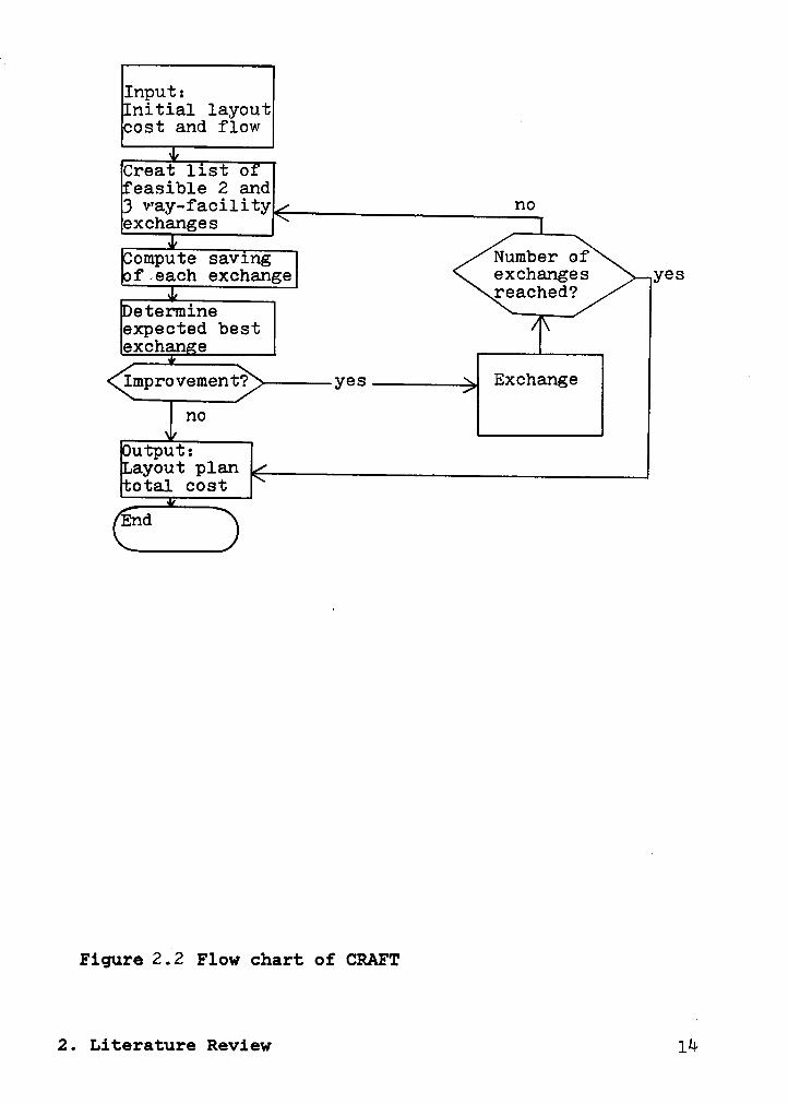
Input:Initial layoutcost and flow

Creat list 0¤easible 2 and3 way—facility noexchanges

ompute saving Number of•f each exchange @X¢h&¤€@S Yes

reached?ßetermineexpected bestexchange

Improvement? Exchange

Output:aayout planotal cost

End

Figure 2Q2 Flow chart of CRAFT

2. Literature Review lk

E111111 IH 1B and D are exchanged.

A EImproved layout C

Pairwise exchanges continue,until no improvement can be made.

Final layoutE

A

Figure;} CRAFT's creation process

2. Literature Review -1-5

formation, cost of movement between floors, and specification

of the movement times. SPACECRAFT is the only method which

allocates departments to locations within a multifloor

building and which considers nonlinear travel times.

PLANET, developed by Apple and Deisenroth (1980), is a com-

puterized approach to facility layout design which utilizes

material flow pattern information. There are two types of

data used in the approach, facility information and material

flow information. Each facility to be entered into the lay-

out must be identified and the area requirements must be

stated. Priority of each facility is also required for fur-

ther use in the facility selection process. Unlike other

computerized methods which require the from-to chart as in-

put, PLANET utilizes an extended parts list instead. Ex-

tended parts list information includes part number, frequency

of move, cost per move, and sequence of movement. These data

are then translated into a format useful to the construction

algorithm, specifically, a from-to chart which represents

costs per unit distance. The objective function of the al-

gorithm is to find a layout alternative with the lowest ma-

terial handling cost possible. The material handling cost

is the sum of the product of cost per unit distance times

‘distance for all facility pairs where distances are

rectilinear and are measured between facility centroids; The

algorithm involves two phases, namely, selection and place-


ment. The objective of the first phase is to select a fa-

cility to be a candidate for use in the placement phase.

Three methods of selection are suggested:

Method A: First select a pair of facilities which has the

highest cost per unit distance. The next facility is chosen

from the unplaced list where the cost per unit distance be-

tween unplaced and placed facilities is the highest.

Method B: Identical to A for the first pair. The remaining

selections are made by considering the relationships between

each of the unplaced list and all facilities in the placed

list. This is accomplished by letting the value in the

placed list column be zero and by adding all the values for

each unplaced row of the unplaced list. The facility with

the highest sum is selected next.

Method C: Adding each row. Facilities are then ranked and

selected according to their sum values.

During the second phase (placement), the selected facility

is placed within the existing facilities. To find the best

location, the selected facility is moved around the perimeter

of the others until the location with minimum change in ma-

terial handling cost is found. The flow chart of PLANET is


depicted in Figure 2.4. PLANET's layout creation process is

depicted in Figure 2.5.

CRAFT, one of the earliest and best improvement algorithms,

has been reworked and implemented in new programs with the

acronym PLOP2, PLOP3, PLOP4 (PLOP stands for Plant Layout

Optimization Procedure). PLOP2 improves an initial layout

by first calculating the change in total cost caused by ex-

changing the locations of all pairs of departments. It then

exchanges the location of the pair of departments that gives

the greatest reduction in total cost. It continues with this

procedure until no further reduction can be made in the total

cost. The general procedure on which PLOP2 is based is ex-

tended to three-way and four-way exchanges of facilities,

which give rise to algorithms PLOP3 and PLOP4 (Lewis andV

Block,l980). Figure 2.6 depicts the flow chart of the PLOP

algorithms.

QUAINT (Quadratic Assignment Implicit N-level Technique) is

a modification of the PLOP series to reduce computing time

while still maintaining the ability to consider swaps at the

third and fourth exchange levels. QUAINT3 initially follows

the same path as PLOP2, but when no two-way swap can give a

further reduction in the total cost, PLOP3 is used to find a

possible three-way swap. When a three-way swap is found, the

program then reverts to PLOP2. With this procedure, QUAINT3

2. Literature Review 'l

18

Input:Facility dataMaterial flow data

Translateextended parts listinto from—to chart

Selectionprocedure

Placementprocedure

no All facilitiesplaced?

yes

Output:Layout plantotal cost

End

Figure 2.4E1ow chart of PLANET


I First p3.II.I' IC„s·

··1I I

Enter E I II C D Search for the

:w best location

· IC. -_ -E

CC

Enter A

I EFinal layout

Figure Z, 5 PLANET's layout creation process


N—way exchangelistCompute costs

mprovement? yes Exchange Q

no E

_ End

N — 2,3,4 for PLOP 2,3,4respectively

Figure 2.6 Flow chart of PLOP A


2-way exchange 2-way exchangeist list

compute costs compute costs

'_ mprovement? Improvement? yes

no no

3-way exchange 3-way exchangeExchange list list Exchange

com•ute costs com•ute costs

yes Improvement? Improvement? yes

no no‘

End M-way exchangelistcompute costs

mprovement? yesno

End

QUAINT 3 QUAINT 4

Figure 2.7 Flow Chart of QUAINT


has the advantage of' being able to make three-way swaps

without the disadvantage of increased computational time.

The flow chart of QUAINT is depicted in Figure 2.7.

In 1980, O’Brien and Barr (1980) developmi a program for

layout design problems which utilizes a sophisticated graph-

ics capability. The program is divided into two main proce-

dures, construction and improvement. The first procedure

(INLAYT) allows a layout to be constructed for situations

such as a new factory or extension, or a major relayout of

facilities. The inputs to this phase include the following:

1. The number of facilities to be considered,

2. The spatial array which consists of equal blocks (i.e.,

if 24 facilities are to be located, the designer must

specify whether he wishes initially to consider a 6*4,

8*3, or 12*2 arrangement),

3. The volume of flow of material traveling between facili-

ties, and

4. A flow factor. (This is a designer-specified variable

between O and 1 to define the level of weighted flow be-

tween facilities which he considers significant.)


Unlike PLANET which requires facility areas, INLAYT does not

require such information because it only assigns facilities

in a spatial array.

The construction procedure starts by ordering the facilities]

according to the sum of weighted flow in and out of each fa-

cility. Each facility is then ranked in, order, and is

grouped·with those facilities for which the weighted flow of

material equals or exceeds the maximum value of weighted flow

found in the weighted flow matrix between any two facilities,

multiplied by the flow factor. The information is presented

on the graphic screen with the spatial array. The designer

can use the light—pen to assign facilities to any location

he wishes, based on information presented, and his judgment.

The procedure ends when all facilities have been assigned to

locations.

The second phase, the improvement procedure (S-ZAKY), begins

from an initial layout which can be an existing one, or that

developed using INLAYT or any other methods. The basic data

required are: 1) the facility specifications including namesu

and areas, 2) the relative locations of departments, 3) the

volume of flow of material between facilities, 4) the detail

of departments with all machinery and other components, and

5) the position of set—down and pick-up points.


Like CRAFT, the algorithm considers the savings in material

handling costs which would result from interchanging the lo-

cations of pairs of facilities, but at each iteration, the

improvement to be obtained from interchanging not one, but

three pairs of facilities, is made. The interchange of three

pairs was adopted after considerable investigation as re-

presenting the best compromise between the improvements ob-

tained and the computing time required. The changes in

location of facilities accepted at each iteration provide the

modified layout to be considered by the following iteration.

The algorithm continues until it reaches its suboptimum sol-

ution in which no further improvements from interchanging

facilities can be found.‘

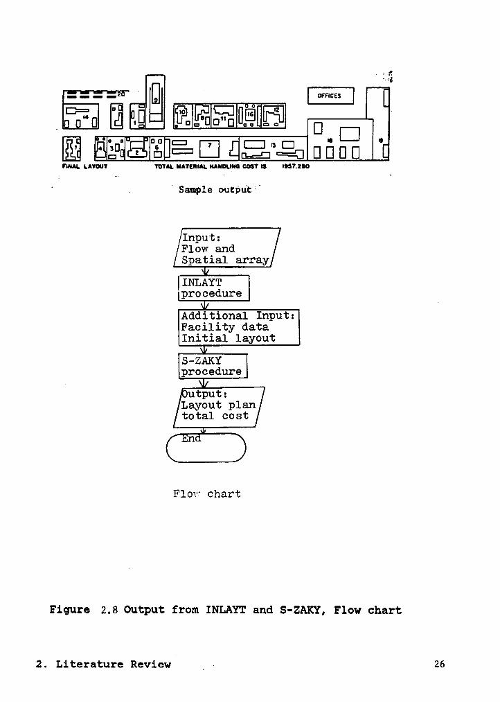
Finally, the computer produces a detail layout plan, unlike

other computer programs which produce only relative locations

of facilities. Figure 2.8 shows a sample of output obtained

from the—INLAYT and S-ZAKY, and the macro flow chart of the

program.

Since all of these computerized approaches utilize quantita-

tive information for their input, the objective is to find a

layout with the lowest total material handling cost. We next

consider computerized approaches utilizing qualitative in-

formation. p


A EEI!}IT ¤!¤ nu : I3 IS

EE [1e:E gg; mmm] IFINAL LAYOUT TUTAL MATERIAL COST IS I957.2S0

° . '·SsmpIe otput°‘

Input:Flow andSpatial array

|1NLAYTprocedure

· Additional Input:Facility dataInitial layout

S-ZAKYprocedure

VOutput:Layout plantotal cost

¤n•

Flow chart

Figure 2.8 Output from INLAYT and S-ZAKY, Flow chart

2. Literature Reviewv I ~ 26

CORELAP, presented by Lee and Moore (1967), is a computerized

construction program based on facility relationships. The

input requirement for CORELAP includes: 1) relationship

chart, 2) number of facilities, 3) area of each facility, andI4) weights for the relationship chart entries. The objective

of CORELAP is to produce a layout which satisfies most re-

lationships. This is measured by the total closeness rating

which is defined as

n n- TPR = E Z P..a..

1=1 j=1 IJ IJ

where

Pij = closeness rating for facility i and j

aij = 1 if facility i and j are adjacent

= O otherwise

Although the weights for the REL chart are arbitrarily de-

fined, CORELAP starts by selecting a facility which is first

placed in the layout. Next, a facility is selected and

placed in the layout where the highest closeness rating is

achieved with the department being placed. The process con-

tinues until all facilities have been placed in the layout.

The process of facility design, including facility selection

and placement, is heuristic and does not guarantee the opti-

mal total closeness rating. Later, new versions of CORELAP

were developed, including CORELAP8 and Interactive CORELAP.


CORELAP8 uses the same concept as the original version, but

provides useful features such as the length-to—width ratio

of the final layout. On the other hand, Interactive CORELAP

provides flexibility in rearranging a layout. Figure 2.9

depicts the flow chart of CORELAP. Figure 2.10 depicts the

flow chart of the facility selection rule used in CORELAP.

Figure 2.11 depicts CORELAP's layout creation process.

ALDEP is a construction and improvement program developed by

Seehof and Evans (Seehof and Evans,1967). Although it uses

data similar to CORELAP, its construction procedure is dif-

ferent from CORELAP. ALDEP develops a layout design by ran-

domly selecting a facility and placing ii: in the layout.

Next, the relationship chart is scanned, and a facility with

the highest closeness rating is placed in the layout. The

ALDEP placement procedure is designed to avoid extreme ir-

regularity in the shape of borders of the layout periphery,

by using the vertical scan methmd of placing facilities.

Basically, the layout area is filled by using vertical strips

having a specified width and length equal to the depth of the

layout. Figure 2.12 depicts ALDEP's layout creation process.

This process is continued until all facilities are placed.

' ‘The improvement proceeds by repeating the entire process and

comparing the resulting score with the existing score. In-

puts to ALDEP are similar to that for CORELAP. In addition,

the user specifies the number of layouts to be generated.


Input:2

REL—chartfacility data

Selectionprocedure

Placementprocedure

All facilities oplaced?

yes

Output:Layout plantotal closeness rating

End

Figure 2.9 Flow chart of CORELAP


Searching forfacility withthe highestsum of closenessrating

A rating esexists?

noE rating

_ exists?

. °°I ratingexists?

IQ

O rating esI exists? '•

noSelecting y@Sfacility withthe next highestsum of closenessratin;

Placementprocedure

Figure 2;lO Flow chart of CORELAP's Selection Rule

2. Literature Review 3Q

First pair I C

I

DI

I

E

Enter EC D

I

Enter B _ Enter A

B

II¤ I EI AI

c D C

_ Fiqure2.ll CORELAP's layout creation process


Vertical Scan /\(

Method(Initial boundary

ALayout CAité”ati”€ I

Layout CAlternative II A

Figure1Z.l2 ALDEP's layout creation process


} Ä

ALDEP will generate multiple layouts and select the one with

the highest total closeness rating.

RMA Comp I is another approach which utilizes the relation-

ship chart. Developed by the staff of Richard Muther and

Associates (Muther,1970), it uses closeness relationships as

input data in a similar manner as ALDEP and CORELAP do. The

logic of selecting facilities is also similar to that used

in CORELAP. RMA Comp I is designed to do by computer what

Systematic Layout Planning (SLP) does manually. This program

recognizes that further manual adjustment of the output is

necessary in order to develop a practical, workable layout,

so it does not try to make a printout showing facilities ad-

jacent to each other as CORELAP and ALDEP do. Its printout

is a space relationship diagram, which attempts to maximize

all closeness rating relationships as shown in Figure 2.13.

The approaches described above were developed primarily by

academicians. The information related to such approaches was

available through academic journals as cited. Since the late

1970s, computer software specially designed for facilities

planning and design began to be available commercially. This

was largely due to the availability of computers with graph-

ics capabilities. Filley (1985) categorizes the software

based on such technologies as follows: 1) decision support

systems (DSS), 2) computer-aided design (CAD) and 3) manage-

2. Literature Review I 33l

• P • • • • • • ¤ • INHIIIIILOIUIM • • P • • • •• • • P P

I_• « • • P « P PPP« • P PP • P

IY,

I•·

xßtll AIIUIB

KQIZQKKXID Iülßiili _• ·•

$:2:2:22:2nuv VNU

PIII. ..IIIIIIZZ§ZIZZIZI• • P PO

·-• • • P PA .•

« • • 5 u • • Oliittll Ä; ^•

P:1

A ZA P _• •A. I••‘¤:••••••~.l

Figure2• 13 Sample output from RMA Comp I

2 . Literature Review 3%·

ment information systems (MIS). Each of these technologies

generally serves a corresponding facilities function, as

follows:

1. DSS-facilities planning. DSS helps make information more

usable. DSS can be applied to issues such as whether to

refurnish or build a new facility, or whether to own or

lease a facility.

2. CAD—facility design. Color and 3-D graphics are now

commonly found in any computer system. Thus, real time

graphic simulations of robotics, material handling sys-

tems, warehousing and production systems can be modeled.

This is the objective of most CAD systems.

3. MIS-facilities management. MIS is typically used to

produce regular reports on assets or facilities utiliza-

tion.

2.1.2 MULTICRITERIA APPROACHES

Multicriteria approaches refer to those where both qualita-

tive and quantitative criteria are simultaneously considered.

Rosenblatt (Rosenblatt,1979) presented a combined quantita-

tive and qualitative approach to the plant layout design

problem. The two objectives, quantitative and qualitative,

} 2. Literature Review 35

which may be conflicting, are to minimize the material han-

dling cost and maximize a closeness rating. However, these

may also be combined into one objective function.

The minimization of material handling cost is formulated as

follows:

— n n n nMin C = 2 E Z Z a., X..X

1=1 3=1 k=1 1=1 llkl ll kl

Subject to

nE X.. = 1 j=1,...,n

i=1 1]

n

jél Xij = 1 1=1,...,n

where

Xij = 1 if facility i is assigned to location j

= 0 otherwise

aijkl = fijdkl if i=k or j=l

= fiidjj+cij if i=k and j=lcij = cost per unit time associated directly with

facility i to location j

djl = distance from location j to location l

fjk = work flow from facility i to facility k

i2. Literature Review k 36

The maximization of closeness rating can be formulated as

follows:

n n n nMax R = 2 2 Z Z w., X..X

1=1 j=1 k=1 l=l lJkl 1J kJ

Subject to

nE X.. = 1 '=l,...,

1=1 lJ J n

nZ Xi. = 1 i=1,...,n1=1 J

Xij =O or 1 for any i and j

where

wijkl = rik if location j and l are adjacent

= O otherwise

rik = closeness rating of facility i and facility k

Thus, a multi—objective formulation is

Min Z = blC - b2R

Subject to

n. . = '=l,...,ii]. X1] 1 j n

) 2. Literature Review 37

nZ X.. = 1 i=l,...,n

i=l ll

Xij = O or 1 for any i and j

bl + bz = 1 and bl, b2 2 O» where bl and b2 are weights assigned to the total cost flow

and total rating score, respectively.

When an alternative is created, the total material handling

cost, C, and the total closeness rating, R, can be calcu-

lated„ These two values are combined through the multi-

objective function. This results in a score which represents

the degree of satisfaction of the layout alternative. This

approach allows a designer to systematically choose the best

layout alternative based on both quantitative and qualitative

information.

Dutta and Sahu (Dutta and Sahu,l982) also consider the

multiobjective problem. They developed a heuristic procedure

for solving the previously described problem. The procedure

takes an initial layout and improves it using a pairwise ex-

change routine.

2.1.3 GRAPH THEORETIC APPROACHES

Graph theoretic approaches refer to approaches using graph

theory in optimizing closeness ratings of adjacent facili-


ties. The Graph theory approach was first introduced by

Seppanen and Moore (Seppanen and Moore,l970) to solve layout

design problems. It attempts to allocate facilities in the

layout so as to give an optimal total closeness rating.

First, the relationship chart is converted into a graph which

is later categorized as planar or nonplanar. The planar

graph can be converted into a block plan layout which gives

an optimal total closeness rating.

Seppanen and Moore (Seppanen and Moore,1975) realized the

difficulties in recognizing the planarity of graphs. Thus,

they introduced a linear string representation and the con-

cept of grammar as basic tools for symbolizing trees and

planar graphs. Algorithms based on graph theory to maximize

closeness ratings as well as to convert planar graphs into

block diagrams were suggested.

2.1.4 MATHEMATICAL MODELING APPROACHES

Mathematical modeling approaches refer to approaches where

. quantitative considerations of a facility layout problem are _

used to construct mathematical models and to represent quan-

titative characteristics of the problem. Francis and White

summarized the various mathematical modeling approaches to

the layout design problem (Francis and White, 1974). These

models have the objective of minimizing material handling


cost which is the sum of the product of distance and cost for

all facility pairs. Generally, the layout design problem is

to assign facilities to locations and minimize total cost.

This problem can be formulated as;

n”n

n nMin X 2 E Z c.. X. X.

i=1 j=1 k=1 h=1 lJkh lk Jh

Subject to

n·E Xik = 1 k=l,...,n1-1

nE X. = 1 i=l,...,n

k=l lk

Xik = O or 1 for any i and k

Jwhere

cikjh = cost of having facility i located at location k

and facility j located at location h

Xik = 1 ,facility i is located at location k

= O ,otherwise

This formulation is a quadratic assignment problem to which

there are no efficient exact methods which can solve

realistically-sized problems.

l2. Literature Review 40

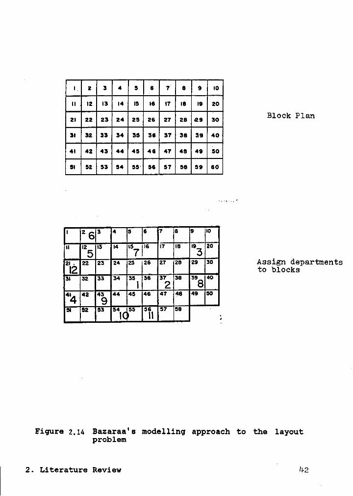
Consequently, Bazaraa (1975) considered the layout design

problem and formulated the problem as a quadratic set cover-

ing problem. His formulation can handle single or multi-

story buildings, facilities with regular or irregular shapes,

designing a layout from scratch, or adding new facilities to

an existing layout. The solution is provided by a branch and

bound optimization procedure. Figure 2.14 shows Bazaraa's

modeling approach to the layout problem.

Chapter 6 will discuss the quadratic assignment problem in

detail.

DISCON is a new approach to the layout problem developed by

Drezner (Drezner,1980). Its objective is to find a layout

with least total cost. However, the DISCON procedure assumes

that facilities have circular shapes, and that distance be-

tween facilities is measured from center to center by

euclidean distance, instead of rectangular distance as in

other traditional layout design programs. The DISCON algo-

rithm includes two phases, dispersion and concentration. The

dispersion phase has the circles (facilities) disperse from

the origin, as the whole system expands. The purpose of the

dispersion phase is to find good initial conditions. The

final solution in this phase gives good starting points for

the second phase which is the concentration phase. At the

end of the first phase, the areas are not touching. In the

second phase, this formation is concentrated or tightened.


Illlll M llßNEEHHB M

M E M E Bl°°" mw¤¤¤¤¤¤ M ¤H¤l¤¤¤¤¤ M ¤¤¤HBHEEE M BBE

IEWWWW WI4 us I6 I7¤ ÜWEF 7,

2,, zv za Assign departmentsI2 ‘¤<> bl¤<=kS

" WEFWWWWW 2EFEWWW" WWF

57 ·WWWEWE g

Figure 2,14 Bazaraa's modelling approach to the layoutproblem

i2. Literature Review u *+2

Assume circular shape and equal size

Initial phase

Dispersion phase

Concentration phase

$9

Figure2„l5 DISCON's process

i

2. Literature Review ~U3

The algorithms in these two phases are based on the

Lagrangian Differential Gradient method suggested by Drezner

(1980). Despite the strange assumptions, Drezner success-

fully used DISCON in an office layout design, where the as-

sumptions of circle—shaped facilities and euclidean distance

were acceptable (Drezner,l980). Figure 2.15 depicts DISCON's

process.

2.1.5 SUMMARY AND CONCLUSION

The section 2.1 has included the literature review in the

area of facility layout design. Four different kinds of ap-

proaches to the layout problem have been surveyed. The com-

puterized approaches are designed to solve the layout problem

with the objective of either minimizing material handling

cost or maximizing the total closeness rating. Heuristic

procedures used in the layout creation process were suggested

‘ to optimize predefined objective functions. The preferred

heuristic procedures are typically determined by the measure

of their computing time. The better computerized softwares

are usually determined by graphics capabilities and user

friendliness. Graph theoretic approaches are the basis of

computerized heuristic procedures. Mathematical modeling

approaches are still in the developing stages. The problem

with mathematical modeling approaches is that there is no

efficient exact methods which can solve realistically—sized


problems. Multicriteria approaches are attempts to include

both qualitative and quantitative criteria in the same ob-

jective function. The multicriteria approaches fail to

standardize the scales of both criteria. Thus, the objective

function may not consistently represent the designer's pref-

erence. The next section surveys decision theory that is

h useful in modeling the multicriteria facility layout problem.

2.2 LITERATURE REVIEW OF DECISION THEORY

One of the most common cases in the evaluation of alterna-

tives is for entities to be composed of two or more compo-

nents, each of which affects the evaluation in question. For

example, a decision maker wants to choose which car to buy.

The decision must be based on two components (attributes),

such as cost and performance. The attributes in this example

cannot readily be combined. However, there exist theories

leading to the construction of measurement scales for com-

posite objects which preserve their observed order with re-

spect•to the relevant attributes (e.g. preference, cost, and

performance). -The theories that lead to simultaneous meas-

urement of the alternatives and their components are referred

to as conjoint measurement theory (Krantz et. al., 1971),U

multiattribute value theory (Keeney and Raiffa, 1976),

multiattribute utility theory (Keeney and Raiffa, 1976),


topology theory (Fishburn,1970), and measurable multiattri-

bute value theory (Dyer and Sarin,1979).

Generally, there are three forms of the aggregation function

used to measure alternatives: 1) additive; 2) multilinear;

and 3) multiplicative. These forms represent the decision

maker's preference. There are more sophisticated forms, such

as the polynomial (mostly applied in physics, Krantz et. al.,

1971), but we restrict ourselves to these three. In most

decision making situations, additive representations have

proven to be the most successful in representing a decision

maker's behavior due to their robustness (Dawes and

Corrigan,1974; Einhorn and Hogart,1975).

2.2.1 MULTIATTRIBUTE VALUE THEORY

Krantz et. al. (1971) presented a classic theorem for the

case of additive multiattribute value models. Before de-

scribing this theorem, we need to introduce the attribute

space X1,...,Xn which describes alternatives and follow it

with some definitions of assumptions underlying the theorem:

1. Weak ordering: All the alternatives can be rank ordered.


2. Independence: H Xi, N={1,...,n} is independent iff,isN

H Xi, for fixed choices of Xi designated as ai, i sisNN—M for some Mc: N, is unaffected by those choices.

3. Restricted solvability: H Xi satisfies restrictedisN

solvability iff, for each i c N, whenever

bl...bi...b¤ 2 al...ai...an 2 bl...bi...b¤,

then there exists bi s Xi such that

b1...bi...bn = a1...ai...a¤

4. Archimedean property: Incremental variation in the level

of each individual attribute is measurable in terms of

measurable incremental variations in the level of other

attributes.

5. Essentialism: The states of each attribute must exercise

some influence on the preference for alternatives.

Any H Xi, N23, is called an additive conjoint structureisN

if all the five conditions hold. A major result from the

theorem of Krantz is that if X1,...,Xn, nz3, is an n-

component, additive conjoint structure, then there exist

real-valued functions vi on Xi, i c N, such that for all ai,

b. s X.,1 1n n

a1...an 2 bl...bn 1ff ii1vi(ai) 2 i;lvi(bi).The following is an outline of the corresponding proof:

i2. Literature Review 47

First, it will be assumed that all components are essential.

That is, every attribute exercises some influence on the

preference value. The next step is to show that there is a

symmetric substructure for which the theorem is true. Let

xo, xl' s Xi be such that x1' > xo and wo', wl z Xj such that

wl > wo'. If xowl = xl'wo', the elements are accepted as

given. If x1'wO' > xowl, then since xowl > xowo', there ex-

ists, according to restricted solvability, an xl s Xi such

that xl > xo and x1wO' = xowl. If xowl > x1'wO', then a

similar argument shows that wo s Xj exists such that wl > wo,

xl'wO = xowl. Dropping all primes, yl, yo s Xk can also be

constructed such that woyl = wlyo, and by independence, it

follows xoyl = xlyo. By continuing inductively, it can be

seen that each two-component substructure bounded by these

elements is symmetric in addition to fulfilling the original

conditions.

Each }%J Xj has an additive representation vi, Vj. In fact

the V1,..., Vn may be selected such that any pair is additive

over the symmetric substructure. To show this, it is suffi-

cient to show for any distinct i, j, k that the group oper-

ations induced on j by i and k are identical. The vj(x)

Values are assigned such that Vj(wojy), where oj represents

concatenation of j component (Krantz,et.al., 1971), equals

Vj(w) + Vj(y). By independence, for any x s Xj, xi§juk(x) =

xixik = ni(x)xjxk. Using this and independence, for x, z s

i2. Literature Review ‘ I 48

Xj, ni(z)(xokz)xk = ni(z)xnk(z) = äi(xoiz)¤k(z) =

ni(z)(xoiz)§k, whence xokz = xoiz. Thus, if vi, vj, and vkare additive representation, there is a linear transformation

of the latter pair into vj, vk. Finally, it is not difficult

to show that vi, vk is also additive. Suppose that x, z 6

Xi, w, r 6 Xj, and y, s 6 Xk are all within the symmetric

substructure and that xwy 2 zrs, then it can be shown that

vl(x) + v2(w) + v3<y> Z v1(z) + v2(r> + v3(S)

This is obvious if x 2 z, w 2 r, and y 2 s, so it can be as-

sumed that at least one inequality is reversed. With no loss

of generality, it may also be assumed that either

(1) x 2 z, w 2 r, s > y or

(2) x > z, w < r, s > y.

(1) If xy 2 zs, then vi(x) + vk(y) 2 vi(z) + vk(s) and from

w 2 r, vj(w) 2 vj(r), so that the result follows by addition

of inequalities. On the other hand assume zs > xy. Since

xs > zs (by (1) above), by invoking restricted solvability,

it implies that there exists a b 6 xk such that zs = xb.Thus, xwy 2 zrs = xrb, so wy 2 rb, whence vj(w) + vk(y) 2

vj(r) + vk(b). From xb = zs, vi(x) + vk(b) = vi(z) + vk(s).

Adding the two inequalities and subtracting vk(b) yields the

result. „

(2) From r > w and s > y, xws > xwy 2 zrs > zws. Thus, by

restricted solvability, there exists c = Xi such that cws =xwy 2 zrs. Thus, vi(x) + vk(y) = vi(c) + vi(s) and vi(c) +


vj(w) 2 vi(z) + vj(r). The result follows by adding ine-

qualities and subtracting vj(c). °

Since strict preference inequalities go into strict numerical

inequalities, the converse follows. A simple induction ex-

tends this result to any n. To extend additivity, use triple

cancellation, reducing x = z to the case where x is in the

symmetric substructure and at most one zi is outside it.

The original version of this theorem was presented by Debreu

(Debreu,1960). Some of his topological assumptions were re-

placed by more general axioms, for example, solvability and

the archimedean property.

Keeney and Raiffa (Keeney and Raiffa,1976) presented condi-

tions for the additive value functions which are abstractions

of the axioms developed by Krantz, et. al (1971). Two inde-

pendence conditions, namely* preferential independence and

mutual preferential independence, are defined below.

The set of attributes Y is preferentially independent (PI)

of the complementary set Z, iff ·T

(Y',Z") > (Y",Z') implies (Y',Z") > (Y",Z") for all Z ,Y ,Y

where Y = {X1,...,XS}, Z = {XS+l,...,XN}

The attributes Xl,...,XN are mutually preferentially inde-

pendent (MPI) if every subset Y of these attributes is pref-


erentially independent of its complementary set of

evaluators.

Given attributes Xl,...,XN, an additive value function

NV(Xl,...,XN) = eg V(Xi) ‘

1-1

exists if and only if the alternatives are mutually prefer-

entially independent (Keeney and Raiffa,1976).

The MPI and PI assumptions are very useful to identify addi-

tive value functions. However, the number of preferential

independence conditions to verify gets very large as the

number of attributes gets only moderately large. In general,

if there are n attributes, there are n(n—1)/2 pairs of at-

tributes that must be preferentially independent of their

respective complements. Gorman saves much potential work by

allowing verification of MPI using only n—l sets of prefer-

ential independence conditions (Gorman,l968a; Gorman,l968b).

His results are stated as follows:

Let Y and Z be subsets of the attribute set S = {X1,...,Xn}

such that Y and Z overlap, but neither is contained in the

other, and such that the union Y U Z is not identical to S.

If Y and Z are each preferentially independent of their re-

spective complements, then the following sets of attributes,


1. Y U Z

2. Y 0 Z

3. Y—Z and Z-Y

4. Y—Z U Z-Y

are each preferentially independent of their respective com-

plements. This saves a lot of work in verifying preferential

independence conditions.

2.2.2 MEASURABLE MULTIATTRIBUTE VALUE FUNCTIONS

The term measurable value function is used, since the dif-

ferences in the strength of preference between pairs of al-

ternatives or, more simply, the preference difference between

the alternatives can be ordered.

Measurable multiattribute value functions provide an alter-

native to cumbersome assessment procedures, since difference

consistency is so intuitively appealing that it could be as-

sumed in most applications (Dyer and Sarin,1979).

Dyer and Sarin (Dyer and Sarin,1979) present the following

V conditions:

2. Literature Review· 52

1. Preferential independence (PI)

2. Mutual preferential independence (MPI)

3. Difference consistent - The set of mutually prefer-

entially independent attributes Xl,...,Xn is difference

consistent if, for all wi, xi s Xi

iff (wi„wi)„(xi„wi> 2* (xi,wi),<xi„wi)

for some wi s Xi and for any i s {1,...,n} and if w = x

then wy =* xy or yw =* yx or both for any y s X.

4. Difference independent - The attribute Xi is differenceindependent of Xi if, for all wi, xi s Xi such that(wi,wi) 2 (xi,wi) for some wi s Xi and(wi,wi),(xi,wi) =* (xi,ii),(xi,§i) for any ii s Xi.

In addition to the four conditions, structural and technical

conditions such as solvability, Archimedean, and essentialism

must hold. Thus, there exist additive value functions over

the alternative set. Fishburn (Fishburn,1970) presented a

similar result, but used persistence conditions which are

" similar to the difference independence conditions.

For multilinear and multiplicative cases, weak difference

independent is defined. XI is weak difference independent


of XI, if given any wI, xl, yI, zI s XI and some WI c XI suchthat

(wI,wI),(xI,wI) 2* (yI,WI),(zI,wI) and

(wI,xI),(xI,xI) 2* (yI,xI),(zI,§I) for any xl s XI.

When XI is weak difference independent of XI, thenv(xI,xI) = g(xI) + h(§i)v(xI,wI)

for any xI, xI, and wI.

2.2.3 MULTIATTRIBUTE VALUE FUNCTION: A BINARY CASE

In some decision situations, alternatives represent combina-

tions of binary attribute states. In the case of contin-

uously measured attribute states, the axiomatic problem is

solved (Fishburn,l970; Krantz, et. al,l971; Keeney and‘

Raiffa,l976; Dyer and Sarin,l979). Deutsch and Malmborg

solved the case of künary attribute states (Deutsch and

Malmborg,1984). The results show the insufficiency of

solvability axioms for an additive conjoint structure in the

case of binary attributes.

The Archimedean property requires that all strictly bounded

standard sequences be finite. The indivisibility of binary

attributes precludes the existence of standard sequences.

Thus, the Archimedean property cannot hold on a binary al-

ternative set. They also show that the restricted

solvability axiom cannot be defined for the binary case.


Alternative conditions for binary attributes are defined as

follows:

1. Discrete Weak Difference Independence (DWDI)

(ei*,Ei),(e&,Ei) 2* (eä,Ei),(e;,Ei) implies that

(ei*,Ei'),(eä,Ei') 2* (e;,Ei'),(éä,Ei') for any Ei' 6 Ei.

2. Mutual Discrete Difference Independence (MDWDI) — The

binary attribute set E satisfies MDWDI if given

eI,eI',eI",eI"' 6 EI and el,(eI,EI),(eI',EI) 2* (eI",EI),(eI"',EI) implies that

(aI.€I')„(aI'.€I') 2* (aI".€I'),(aI"'„€I') far any EI.EI' where I C N. ‘

3. Discrete Difference Consistency (DDC) - The binary at-

tribute set E satisfies DDC if it satisfies monotonicity

and if for all I C N and

EI 6 EI, e = e' implies that e,e" =* e',e".

4. Discrete Compensatory Independence (DCI) — This condition

is defined as follows:

If (eI,eJ,EIJ) > (eI',eJ',EIJ) and eI' 2 eJ

than (aI,äI).(aI'.€I) 2* (aJ',€J).(aJ.€J)for all EIJ 6 EIJ, EI 6 EI, EJ 6 EJ and I,J c N.


When the four conditions hold, there exists an additive rep-

resentation over the alternative set

nv(e) — iilciei.

Multilinear form requires DWDI. When ei is DWDI to its com-

plement, we have

· v(ei„äi) = q(¤i) + h(ei)v(ei'„€i)

The MWDI must hold for multiplicative form of

”n

Xv(e) + 1 = H (Xv.(e.) + 1)i=1 1 1

Readers who are interested in the proof of these theorems are

referred to Deutsch and Malmborg (1984).

2.2.4 SUMARY AND CONCLUSION

Three essential results including those pertaining to:

multiattribute value theory, measurable multiattribute value

functions, and multiattribute value functions for the binary

case have been presented. Multiattribute value theory re-

presents the case when all the attributes are continuous.

1 The measurable multiattribute value function theory provides


an alternative axiomatic system that is applicable to con-

tinuous attributes but based on different independence con-

cepts. The multiattribute value function theory for the

binary case is useful in many decision making situations

since the nature of attributes in many problems may not be

continuous. As we will show in the next chapter, layout de-

sign is not in general a continuous attribute problem.

In the next chapter, we will show that the facility layout

problem represents a special class of decision problems for

which xu> existing axiomatic foundation has been defined.

Further, it is shown that decision analysis concepts can be

easily applied to the layout problem in the context of opti-

mal and heuristic strategies for layout creation. In addi-

tion. to developing such axiomatic foundations and layout

creation strategies, a decision support technology for their

implementation is presented in Chapter 4.

*


3. DECISION THEORETIC APPROACHES TO THE GENERAL PLANT LAYOUT

PROBLEM

3.1 INTRODUCTION

In the previous chapter, literature in the area of facility

design and measurement theory was surveyed. This survey

provided background in hmth of these areas. In this re-

search, measurement theory is applied to evaluate and design

layout alternatives. As will be described in this chapter,

measurement theory is used to construct models that represent

the layout designer's preferences. Proper implementation ofuthese models leads to an efficient facility design approach.

3.1.1 STATEMENT OF NEED FOR THE ALTERNATIVE APPROACH

The layout design problem is complex in nature. It involves

many conflicting criteria such as improving worker safety,

enhancing system flexibility, improving labor satisfaction,

and reducing material handling cost, material flow, and dis-

tance travelled. Some of these criteria are quantitative in

nature while others are qualitative. Typically, layout de-

sign approaches consider the criteria of reducing material

handling- cost, material flow or distance travelled. Ap-

1 3. Decision Theoretic Approaches to the General Plant

¥

Layout Problem 58

proaches, such as CRAFT and SUPERCRAFT, utilize quantitative

information regarding material flow, cost, and distance.

Layouts designed by these approaches require major adjust-

ments of the final plan to satisfy other qualitative crite-

ria. ALDEP_ and CORELAP utilize qualitative information

regarding the relationships among activities (REL chart).

The designer provides the degree of importance for pairs of

departments to be adjacent. The objective is then to create

a layout which satisfies as many of these relationships as

possible.

An approach is needed that explicitly addresses the multi-

criteria nature of the facilities design problem. One pos-

sibility is to utilize decision theory to convert qualitative

and quantitative information into readily measurable forms.

This approach should also provide a precise way of utilizing

closeness ratings so that they can be applied effectively in_

the evaluation and construction phases of layout design.

3.1.2 OBJECTIVES OF THE ALTERNATIVE APPROACH

Recognizing the multicriteria nature of the facility layoutv

problem, general objectives of this research effort are to

develop:

3. Decision Theoretic Approaches to the General PlantLayout Problem S9

1. a methodology to design and evaluate facility layouts,

and

2. a suitable technology to implement such a methodology.

The methodology is a decision theoretic approach which uti-

lizes measurement theory in measuring both quantitative and

qualitative criteria in a systematic fashion. The first step

of the methodology is the development of an extension of the

REL construct to incorporate multiattribute value functions.

q The extension of the REL construct is to provide a more pre-

cise statement of closeness ratings. These values can better

represent designer preferences. Following this, measurement

theory is utilized in combining closeness rating scores, ma--

terial handling cost and other specified criteria into a

single value. This value represents overall merit for a

layout alternative.

The second objective is achieved by designing a proper deci-

sion support system to implement the methodology. The deci-

sion support system is developed by studying the man machine

interaction with the objective of utilizing both man and ma-

chine effectively. The system is then programmed on an IBM

PC for implementation.

. 3. Decision Theoretic Approaches to the General PlantLayout Problem 60

3.1.3 OVERVIEW OF THE CHAPTER

In the section that follows, measurement considerations used

for preference modeling and evaluation of layout designs are

described. These will address the multiattribute nature of

facility layout problems, including the need to consider both

continuous and discrete attributes in problems, the insuffi-

ciency of the present axiomatic system, and an alternative

axiomatic system for the mixed case. This is followed by a

description of a decision theoretic approach to facility

layout which includes an extension of the REL construct,

utilization of multiattribute value functions in layout cre-

ation, and overall multiattribute evaluation of layout al-

ternatives.

3.2 MEASUREMENT CONSIDERATIONS

The purpose of this section is to define facility design as

a multiattribute problem and investigate it from a measure-

ment theory point of view. We also show that the problem

cannot be modeled using any existing axiomatic system. An

alternative axiomatic system is then suggested.

3. Decision Theoretic Approaches to the General PlantLayout Problem 61

3.2.1 THE MULTIATTRIBUTE NATURE OF THE FACILITY LAYOUT

PROBLEM

In a facility layout problem, the designer must decide where

· to locate facilities in order to satisfy a set of criteria.

Such criteria include material handling cost, flexibility for

product change, flexibility for expansion, safety, labor

satisfaction and supervision. There are numerous studies

devoted to the criterion of minimizing material handling

costs. The criterion is well defined and can usually be

measured effectively. There are many mathematical models

developed that can represent this measurement. However,

other criteria mentioned above cannot be measured objectively

because they are ill-defined and/or too complex to be mod-

eled. This type of criteria are rated subjectively by the

experienced designer. Facility design is therefore a multi-

attribute problem since both well defined and ill defined

criteria should be considered when designing layout alterna-

tives. Explicit recognition of such criteria has the poten-

' tial to lead to an effective layout design methodology.


3.2.2 THE NEED TO CONSIDER THE MIXED CONTINUOUS AND DISCRETE

MULTIATTRIBUTE PROBLEM

Given that facilities layout is a multiattribute problem, we

can take a closer look at each attribute or criterion. Sup-

pose that the design criteria under consideration are mate-

rial handling cost, flexibility, safety, and ease of

supervision. All of these criteria are relevant for most

facility design problems. Material handling cost is a con-

tinuous attribute, since any small change in arrangement

usually results in an increase or decrease in material han-

dling cost. On the other hand, flexibility is a subjective

criterion and must be rated by the designer. The specifica-

tion of flexibility may be easily perceived by the designer

if the scale of flexibility is divided into discrete inter-

vals like low, medium, and high. The designer can then ac-

curately rate flexibility based on experience. If

flexibility is scaled between O and 100, the designer would

have difficulties relating scaling values to his experience.

Thus, such criteria should assume approximate discrete val-

ues. A similar assumption can also be applied to the safety

criteria. Consequently, we can. conclude that a facility

layout problem involves both continuous and discrete attri-

butes.}


3.2.3 THE INSUFFICIENCY OF PRESENT AXIOMATIC SYSTEMS

Axiomatic systems for additive, multiplicative, and multi-

linear decision model forms have been developed by Krantz,

et. al.(1971). _Keeney and Raiffa (1976) have presented con-

ditions which are the abstract of those axioms. These con-

ditions are mutual preferential independence (MPI) and

preferential independence (PI). These conditions can be used

to verify the consistency of additive, multiplicative, or

multilinear preference models with a decision maker's stated

preferences. In addition to these conditions, there are four

technical conditions which must hold for an additive model

(Krantz, et. al., 1971). These are referred to as weak or-

dering, essentialism, the Archimedean property, and re-

stricted solvability. Deutsch and Malmborg

(1984)demonstratedthe insufficiency of the axiomatic system stated

above for application to the binary attribute problem. They

showed that two technical conditions, namely, weak ordering

and essentialism, can be defined for the binary multiattri-

bute case, while the restricted solvability and the

Archimedean property cannot be defined. This leads to the

conclusion that the existing axiomatic system can apply to

only continuous attribute values. Thus, they developed an

alternative axiomatic system for the binary multiattribute

case. The development resulted in four conditions: 1) dis-

‘3. Decision Theoretic Approaches to the General PlantLayout Problem 64

crete weak difference independence (DWDI), 2)mutua1 discrete

weak difference independence (MDWDI), 3) discrete difference

consistency (DDC), and 4) discrete compensatory independence

(DCI).

To demonstrate the insufficiency of the present axiomatic

systems for the mixed attribute problem, it is enough to show

the insufficiency of Krantz's additive conjoint structure for

the binary case and the alternative axiomatic system (Deutsch

and Malmborg, 1984) for the mixed attribute case. The binary

attribute case as well as the continuous case is a special

case of the xnixed attribute case. The structure of the

multiattribute classification is shown in Figure 3.1.

Before proceeding with the discussion, we first need to es-

tablish some terminology. Let E= E1,...,En be a consequence

space where Ei is the ith binary attribute and (e1,...,en)

is a specific consequence. The attribute Ei can assume only

two levels given by the most preferred state, ei*=1, or the

least preferred state, ei=O, for i s N={1,...,n}. The term .

E is defined to mean ·H Ei, I c.N and ei is a specific level

of Ei.ls?

Now, by essentialism, which thereby

requires that Vi(ei*) > Vj(e3) and Vi(ei*) > Vj(eE), and thus

3. Decision Theoretic Appraacbes to the General PlantLayout Problem 65

Mixed attributes problembinary, discrete, and continuous

I*

Discrete Continuousmultilevel and binary

. ** .Binary Multilevel

* Krantz,et. al. (1971), Keeney and Raiffa (1976)

** Deutsch and Malmborg (198M)

Figure 3.1 Multiattribute value function classifica-tions ‘


Vi(ei*)+Vj(ej*) > Vi(e;)+Vj(e;) = O, for an arbitrary zero

point of the interval scaled V values. However, if (ei*,€;)

2 (ej*,e;), then by transitivity and independence we know

that Vi(ei*) 2 Vj(ej*) for i,j s N. To extend this result

somewhat, suppose that there exist ei,ei' s Ei, ej,ej' s Ej

and eI,eI' s EI, such that (ei,ej,eI) 2 (ei',ej',eI'). The

question essentially asks if the following condition holds,

that is:

I(1) Vi(ei)+Vj(ej)+VI(eI) 2 Vi(ei )+Vj(ej')+VI(eI').

This result follows directly if ei2ei', ej2ej', and eI2eI'.The other possibilities are one of the two general forms,

namely,

(2) a: (eizei', ejzej', eI'>eI), b: (ej2ej', eI2eI', ei'>ei)

or c: (ei2ei', eI2eI', ej'>ej)

and

(3) x: (eizei', ej'>ej, eI'>eI), y: (ej2ej',ei’>ei,

eI'>eI)

or z: (eI2eI', ei>ei', ej'>ej).

For the cases described by (2), restricted solvability de-

fined on E does not preclude (1). For example, consider

version a. Here, if (ei,eI,e§) 2 (ei',eI',e;), then Vi(ei)

+ VI(eI) 2 Vi(ei') + VI(eI'), and since ej2ej', then Vj(ej)

2 Vj(ej') and (1) is obtained by adding these two inequal-

ities. Alternatively, if (ei',eI',e3) 2 (ei,eI,e§), then by

restricted solvability there exists eI" s EI such that(ei',eI',eB) = (ei,eI",e;) so that (ej,eI,e;) 2 (ej',eI",e;)


implying that Vj(ej) + VI(eI) 2 Vj(ej') + VI(eI"). Using the

result that (ei',eI',e;) = (ei,eI",eE),·we obtain Vi(ei) +

VI(eI") = Vi(ei') + VI(eI'). When added to the previous in-

equality, (1) is obtained upon subtracting VI(eI") from both

sides of the resultant inequality. However, a problem arises

with respect to cases described by (3). Consider version x

from which it follows that (ei,ej,eI') > (ei,ej,eI) 2

(ei',ej',eI') > (ei',ej,eI). Restricted solvability requires

that there exists ei" s Ei such that (ei",ej,eI') =(ei,ej,eI) 2 (ei',ej',eI'). However, (l) in this case im-

plies that ei>ei' and (ei",ej,eI') = (ei,ej,eI) implies that

ei>ei" for version x. This is impossible since it implies

that ei> ei"> ei' and attributes can assume only two levels

by definition. Thus, restricted solvability with respect to

binary attributes cannot be defined to show that E has an

additive conjoint structure and an alternative axiomatic ba-

sis for value functions is needed in this case.

3.2.4 AN AXIOMATIC SYSTEM FOR THE MIXED CASE

Most of the facilities design problems of interest have been

shown to be mixed attribute problems and due to the insuffi-

ciency of the present axiomatic systems for this case, weV

develop an axiomatic system for the mixed case. The detail

of the alternative axiomatic development is one major objec-

i


tive of this research. The development of axiomatic systems

is presented in Chapter 5.

3.2.5 SUMMARY AND CONCLUSION

This section has shown that the facility layout problem is a

multiattribute problem having both continuous and discrete

attributes. We refer to this problem as the mixed continuous

and discrete multiattribute problem. The insufficiency of

the present axiomatic system to support the mixed problem has

been demonstrated. In the course of this research efforts

will be directed toward development of an alternative axi-

omatic system defined on a mixed attribute set for additive,

multiplicative, and multilinear forms.

3.3 APPLICATION OF DECISION THEORY TO THE LAYOUT DESIGN

PROBLEM

As stated earlier, facilities design involves both quantita-

tive and qualitative factors. However, there are few re-

ported research efforts that apply a decision theoretic

approach to this problem. Most of the approaches are di-

rected to quantitative factors. Some approaches, e.g. ALDEP

and CORELAP, consider qualitative factors by using the ac-

tivity relationship chart, and they construct layout alter-.


natives based on activity relationship information. Few

studies, for example Rosenblatt's (1980), consider both fac-

tors. Rosenblatt used scores from each objective function

multiplying those by weights to reflect the importance of

each objective. This was then used in an additive scoring

model.

However, from the measurement theory point of view, the

method of combining the two objectives suggested by

Rosenblatt (1980), cannot really represent the merit of the

layout alternative, since the two objectives have different

scaling standards. In order to combine the two objectives,

measurement theory must be applied to convert both scaling

standards into the same type, and find an appropriate combi-

nation·ru1e, for example, additive and multilinear. Section

3.3.3 is devoted to this subject.

Aside from the role of measurement theory stated in the pre-

vious paragraph, it can also be applied in constructing the

REL chart. Traditionally, all pairwise combinations of re-

lationships are evaluated, and a closeness rating (A,E,I,O,U,

or X) is assigned to each facility pair. Then, arbitrary

values are assigned to closeness ratings, for example,

CORELAP uses A=6, E=5, I=4, O=3, U=3, and X=1. Again this

fails to represent an accurate closeness rating since the


numerical values are arbitrarily assigned. Section 3.3.1 is

devoted to the use of measurement theory in constructing the

REL chart.

3.3.1 EXTENSION OF THE REL CONSTRUCT TO INCORPORATE

MULTIATTRIBUTE VALUE FUNCTIONS

The proposed extension of the REL will provide more insight

into the facility layout problem and more meaningful numer-

ical values for closeness ratings.

It is a fact that the closeness rating assigned to any

pairwise combination of' facilities is typically based on

multiple criteria. The purpose of extending the REL con-

struct is to incorporate such reasons. This extension may

be viewed as considering a set of criteria which can be sat-

isfied by having adjacent facilities. Such criteria can in-

clude convenience, common personnel, ease of supervision,

flow of materials, etc. Some of them are listed in Appendix

D.

A preference model based on the adjacency criteria is pre-

sented. The model can have additive, multiplicative, or

multilinear forms depending on the satisfaction of the inde-

pendence conditions with respect to the decision 1naker's

&

3. Decision Theoretic Approaches to the General Plantb

_·Layout Problem 71

preferences. Let Xl,...,Xn be the criteria under consider-ation, for example, convenience, common personnel, ease of

supervision, etc. If the conditions across the attributes

for the additive form hold, we have a preference value for

any paired facility i,j as follows:

Preference value (pij) = clV1(Xijl)+...+c¤Vn(Xijn)

where

ck = scaling constant describing the relative importance

of attribute k,

Vk(Xijk) = marginal value function describing the preference

effects of Variation in the level of individual

attribute k of department pair i,j.

The designer inputs desired levels of each attribute for each

facility pair. For n facilities with m attributes, there are

a maximum of m*n*(n—l)/2 specifications. For 40 facilities

and 4 attributes, there are a maximum of 3120 specifications.

However, the actual number of specifications would not reach

this number, since not all attributes in any pair i,j are

perceived as relevant and/or sufficiently important. The

results from the model are numerical values representing

closeness ratings. The method presented provides a finer

i

3. Decision Theoretic Approaches to the General Plant ‘

Layout Problem 72

scale than the existing A, E, I, O, U, X rating and arbi-

trarily assigned numerical values.

3.3.1.1 EFFICIENT ASSESSMENT OF THE VALUE FUNCTIONS

Theoretically, the value function for each attribute may not

be assessed independently due to potential interdependence

among attributes; thus, an assessment of joint value func-

tions should be conducted. This joint value function is

similar to a joint probability function. When appropriate

_ independence conditions across all attributes hold, we are

able to evaluate and assess value functions independently;

such a function is called a marginal value function. The

efficient way of evaluating marginal value functions is the

" mid—value splitting technique (Keeney and Raiffa, 1976); an-

other one is the SMART technique due to Edwards (1971).

Upon completing the assessment of marginal value functions,

we assess scaling constants. The scaling constants represent

an importance weight for attributes. The assessed marginal ·

value functions and scaling constants as well as an aggre-

gation form represents the closeness rating function for the

problem.

‘


3.3.1.2 OVERVIEW OF ASSESSMENT SOFTWARE

An assessment software package is developed for the imple-

mentation of the method. The software is capable of assess-

ing marginal value functions and scaling constants for an

additive preference model. In addition, the software uti-

lizes interactive graphics to simplify the assessment proce-

dure. The procedure consists of the following general steps.

1. Collect information about the attributes.

2. Rate the attributes on a scale between 1 to 100.

3. Normalize the ratings determined in step 2.

4. If reassessment of scaling constants is required, go back

to step 2. Otherwise, proceed with the assessment of

marginal value functions.

5. Develop marginal value functions.

6. Store the scaling constants and value functions.

Once the preference matrix has been completed, layout cre-

ation proceeds. This is described in the next section. _.

3. Decision Theoretic Approaches to the General PlantLayout Problem ° 74

3.3.2 UTILIZATION OF THE MULTIATTRIBUTE VALUE FUNCTIONS IN

LAYOUT CREATION

This section describes how closeness ratings can be used in

the layout creation process. Then, advantages of the pro-

posed method over existing ones are discussed.

3.3.2.1 DESCRIPTION OF THE PROCEDURE

Having developed the preference values for all pairwise fa-

cilities from the previously described methodology, we use

these values as evaluators in the layout creation stage.

To evaluate the degree of satisfaction, total preference

(TPR) is defined as follows:

n nTPR= 2 2 p../d..

1=1 j=1 1J 13

where

dij = rectilinear distance between department centroids.

pij = closeness rating of pair i,j.

Our goal is to create a.layout which gives the highest TPR

possible since this indicates fulfillment of adjacency re-

quirements. A computer program will be developed to create

facility layouts using these closeness ratings. The software


will utilize a closeness rating matrix and TPR as evaluators

during the creation process. The initial layout creation

procedure is described in chapter six.

3.3.2.2 ADVANTAGES OVER EXISTING METHODS

Existing software, such as CORELAP and ALDEP, use a closeness

rating which is arbitrarily assigned. The scales used are

divided into 6 levels, A, E, I, O, U, and X. They use a

similar selection and. placing rule as illustrated in ‘the

proposed method. However, it is more likely that ties in the

selection and placing process would occur as a consequence

of their rough scaling. The method presented utilizes a

finer scaling system. Thus, closeness ratings from our pro-

posed method more closely represent the actual preference of

the designer. In situations where most facilities are re-

quired to be adjacent, the finer scaling system can easily

distinguish which facility pairings are preferable.

3.3.3 OVERALL MULTIATTRIBUTE EVALUATION OF LAYOUT

ALTERNATIVES

In the overall evaluation step, several evaluation criteria

can be defined. Two of them are total preference rating and

material handling cost. Others may be flexibility, ease of

i


expansion, and appearance. The following evaluation model

is used which provides ranking scores.

nS. = Z a.v (c..)1 j=1 J J 1]

where

Si = score for alternative i,

cij = specification of criterion j for alternative i,

aj = scaling constant of criterion j in the overall

evaluation model, and

vj(cij) = marginal value function of criteria j.

The computer calculates the total preference rating and totalA

material handling cost for every alternative. Evaluations

for subjective criteria are provided by the designer. These

evaluations are aggregated by the evaluation model. Layout

alternatives are then ranked based on their scores. The

layout with the highest score represents the most preferred

layout.

3.4 THE MAIN STEPS OF THE PROPOSED PROCEDURE FOR LAYOUT

DESIGN „

The procedure described above for the layout design problem

can be summarized in the following eight steps.


Step 1. Determination of closeness rating.

This step evaluates closeness ratings of pairs of depart-

ments.

Step 2. Determination of value functions and scaling

constants.

In this step, the marginal value functions and scaling

constants for closeness related criteria are evaluated.

Step 3. Determination of preference ratings.

The closeness ratings of step (1) are converted in this

step into preference scales called preference ratings.

Step 4. Determination of preference matrix.

The preference ratings of step (3) are then converted into

preference value as described in section 3.3.1.

Step 5. Layout creation.

The layout is then created as described in section 3.3.2,

utilizing the preference matrix of step (4) as evaluators.

Step 6. Assessment of value functions and scalingI

constants for the overall decision criteria.

Next, the designer generates value functions and scaling

. constants for the overall decision criteria.


Step 7. Computations of final scores.

Finally, scores for ranking layout alternatives are com-

putmd as described in section 3.3.3 using the information

gathered in steps (5) and (6).

Next, we illustrate these steps on an example problem. Con-

sider a problem containing four departments. There are two

closeness related criteria of interest, namely, the flow of

material and the necessary contact between departments.

Their values are as follows.

Flow N•cessary contact1 2 3 4 1 2 3 4

1 — 50 30 10 1 — 0 1 02 50 - 5 20 2 0 — 0 13 30 5 - 10- 3 1 0 - 04 10 20 10 - 4 0 1 0 -

The flow of material between departments i and j is measured

here in terms of the number of trips made between the de-

partments. For example, the material flow between depart-

mente 1 and 2 is represented by 100 trips with 50 trips each

way. The necessary contact between departments is important

because of technological constraints and is represented above

by 0 and 1. For example, a contact is necessary between de-

partments 1 and 3 and is not necessary between departments 1

and 2. This constitutes step (1) described above. Next,

}_ 3. Decision Theoretic Approaches to the General PlantLayout Problem 79

information is gathered regarding the designer's value func-

tions and scaling constants. Assume these are as follows for

the two criteria selected for this problem.

Flow Contact necessaryscaling constant=0.3 scaling constant=0.7

1 1

0 00 50 0 1

The preference functions map closeness ratings into prefer-

ence ratings, for example, 50 trips in the value function for

flow represents preference rating of 1 and 0 trip represents

preference rating of O. Scaling constants represent weights

of each criteria. The scaling constants for the criteria of

flow and necessary contact are 0.3 and 0.7 respectively. In

other words, the necessary contact is more than twice as im-

portant than the flow. Using these functions, the closeness

ratings of the above example are mapped into the following

preference ratings.

Flow Contact necessary1 2 3 4 1 2 3 4

1 - 1.0 0.6 0.2 1 — 0 1 02 1.0 - 0.1 0.4 2 O - 0 13 0.6 0x1 — 0.2 3 1 0 - 04 0.2 0.4 0.2 - 4 O 1 0 -

The preference ratings of the two criteria shown above are

next combined into single values, called preference values,


using the scaling constants. The combination rule of the two

criteria for this example problem is an additive one. For

example, the preference value between departments 1 and 3 is

O.6(O.3) + 0.1(0.7) = 0.88. The preference values so ob-

tained are shown below.

Preference value matrix

1 2 3 41 — 0.30 0.88 0.082 0.30 — 0.03 0.823 0.88 0.03 - 0.064 0.06 0.82 0.06 —

Next, the layout alternatives are created and the preference

value matrix is used as described in section 3.3.2 for eval-

uating alternatives. In this example, two layout alternative

are created which have the TPR of 3.5 and 2.6 as shown below.

Layout alternative #1 Layout alternative #2TPR=3 . S TPR=2 . 6

1 1 2

E 3 E 3The TPR score represents the preference rating of the above

two alternatives when all the closeness related criteria are

considered. In case some other subjective criteria should

be considered for the overall decision, we need to determine

value functions and scaling constants for these criteria.

For the example problem, value functions and scaling con-

i


stants for the closeness related criteria and some other

subjective criteria are as follows.

Closeness related criteria Other subjective criteriascaling constant=0.6 scaling constant=0.4

0 0

lV lgO 10 0 10

The TPR score for layout alternatives were computed earlier.

The designer then rates each alternative based on a scale of

1 to 10. In this example, assume layout alternatives 1 and

2 are rated as 8 and 6, respectively. The two scores namely,

TPR and the designer's rating, are mapped into preference

scales. Both the TPR and the designer's rating scores are

then combined. The results are shown below regarding the

overall preference rating of the two layout alternatives in

consideration.

$(1) = O.6(O.3S) + 0.4(0.80) = 0.53$(2) = 0.6(0.26) + 0.4(0.60) = 0.40

The designer can now select the final layout based on these

scores. In this case, layout alternative 1 is better.


3.5 SUMMARY AND CONCLUSIONS

This chapter has described a decision theoretic approach to

a facility layout problem. First, the extension of the REL

chart is presented by using multiattribute value theory to

construct a closeness rating function for any pair of adja—

cent facilities. The results from the closeness rating val-

ues are represented in a finer scale than those suggested in

such approaches as CORELAP and ALDEP. A finer scale and TPR

presented would capture designer preferences better than the

methods available in the literature, since the TPR presented

includes relative distances between any pair·of departments.

Finally, an overall evaluation of layout alternatives is

suggested by constructing a scoring model across evaluation

criteria. The model is based on multiattribute value theory.”


4. A DECISION SUPPORT SYSTEM FOR FACILITY LAYOUT

Most approaches to facility design have been unsuccessful as

a consequence of not involving the designer sufficiently in

the design and evaluation process. Therefore, there is a

need for a decision support system to aid design and evalu-

ation of facility layouts that involves the designer. Such

a decision support system should recognize that the decision

maker's judgment is a critical component to be utilized in

the layout creation process.

The first step is to identify the decision criteria. There

are different criteria and different degrees of impact for

criteria in various design situations. Later, the layout

alternatives are designed based on the criteria defined. The

objective of the decision support system is not to construct

an approach and let it create the layout alternative, but to

allow human judgment to have an important role through the

design process. Consequently, the designer may utilize his

judgment to arrive at an ideal layout. His judgments are

determined through the use of decision models, multiattribute

value functions for REL and an overall multiattribute evalu-

ation function, as presented in section 3.3.

4. A Decision Support System'for Facility Layout 84

4.1 THE MAN MACHINE CONCEPT OF DECISION MAKING APPLIED TO

FACILITY LAYOUT

Since humans find it difficult to integrate a large amount

of information in a consistent manner, what is needed is an

aid to help overcome these specific limitations. Computers

can be used to effectively moderate these limitations. They

have the capability of quickly converting a large amount of

information, through use of a man made model, into simple and

easy to interpret forms. The user then proceeds with an

action, based on his judgment and information provided by the

computer. Again the computer performs tasks corresponding

to the designer's reaction. These interactions continue un-

til an acceptable output or outcome is met. Thus, the man

and 1nachine concept is applied to aid facility design. The

following subsections describe comparative advantages of man

versus machine. Later, the overview of the decision support

system represented by a man-machine interaction diagram is

presented.

4.1.1 DESCRIPTION OF COMPARATIVE ADVANTAGES

Due to the complex nature of the facility layout problem, a

system applied for solving the problem must have the follow-

ing capabilities.

4. A Decision Support System for Facility Layout 85

1. Perform fixed logic - search and construct a layout which

gives the lowest material handling°cost and handle a

large amount of data.

2. Utilize human creativity and experiences - have the de-

cision maker evaluate the more complicated and ill-

defined criteria.

The interactive computer system developed in this research

has both capabilities, and effectively combines these human

and machine capabilities. In a layout design problem, human

capabilities are necessary for the evaluation of ill-

structured criteria, creative design, and an realistic and

practical layout. On the other hand, machine capabilities

are needed for the creation of the initial layout according

to fixed logic which includes searching and. calculating,

computing material handling cost, total preference, and final

evaluation scores. If we combine human and machine capabil-

ities properly, we have an effective system to design and

evaluate a facility layout. '

4.1.2 OVERVIEW OF THE DECISION SUPPORT SYSTEM

The decision support system is implemented on a microcomputer

« system. The IBM PC system was chosen because of its wide

spread use. Figure 4.1 shows the man—machine interaction,


and the information flow at each interaction stage. A com-

puter program is designed following this concept.

The key to a good decision support system is to enhance human

performance by providing the designer with the right infor-

mation at the right time without overloading him. Generally,

a user should not perform any tasks that can be programmed

more effectively for the computer.

4.2 DESCRIPTION OF THE DECISION SUPPORT SYSTEM

The purpose of this section is to describe the computer

software developed for this°research. The software is based

on the man-machine interaction diagram in Figure 4.1.

4.2.1 DATA REQUIREMENTS

The initial data requirements of the program are facility

specifications that include facility lengths, widths, names,

and requirements for all facility pairs. The value function

components, which are scaling constants and marginal value

functions, are also required as initial input. Later in the

evaluation stage, scaling constants and value functions for

overall decision criteria are required for a complete evalu-

ation.

i


Facility specificationspreference specifications

Value functions Closeness ratings‘@Initial layout

TPR Adjustment Layout arrangements

‘ Layout alternatives

Criteria scores

Evaluation functio Ranking scores

@FigureU«J„ Man-machine Interaction for Facility Layout

Problem


These requirements are considered to be fixed data, since

they represent characteristics of the problem and the de-

signer's behavior.

4.2.2 USER INTERACTION

The software is designed to enable the designer to interact

at any stage of the program. The designer can switch to any

part of the program to change or edit data as he wishes.

However, the most important interaction occurs during the

layout creation phase where the designer provides the lo-

cations of facilities based on his judgment. This inter-

action allows the designer to use his creativity in arranging

the facilities based on other criteria. Then his judgment

will move towards optimal design.

4.2.3 ASSUMPTIONS OF THE MODELING APPROACH

The major assumptions that underlie the software development

are as follows.

1. Preference models are additive - this allows the user to

assess value functions independently.

2. Distance between department centroids is rectilinear

}4. A Decision Support System for Facility Layout 89

3. Department sizes are equal - this is the assumption used

in the methodology for finding relative department lo-

cations.

4.2.4 INTERFACING THE MODULES OF THE SYSTEM

The software package is divided into three phases which link

to eleven subprograms. These are:

1. Data Acquisition

a. Scaling constant assessment

b. Marginal value function assessment

c. Facility specification

d. Adjacency requirement input

e. Preference matrix computation

2. Layout construction

a. Initial layout construction

b. Layout editing ·

4. A Decision Support System for Facility Layout 90’“

3. Evaluation

a. Scaling constant assessment

b. Marginal value function assessment

c. Criteria specification

d. Final scores computation

The designer can gain access to any part of the main menu.

From the submain menu, the user can go back to the main menu

or run any modules in that menu.

4.2.5 ADVANTAGES OF THE SYSTEM

The proposed system has the following major advantages over

existing computer aided facility layout design systems.

1. It utilizes the man-machine performance concept which

results i11 a better decision support system for the de-

signer. .

2. It includes layout creation and evaluation in one pack-

age.

i


3. It is implemented on a microcomputer.

4. It considers the multicriteria nature of the facility

layout problem.

5. It uses an extension of the REL construct to measure

closeness ratings.

4.3 SUMMARY AND CONCLUSIONS

This section has described the decision support system de-

signed for the facility layout problem. It is, in fact, an

interactive computer system designed to be a tool for layout

design. The capabilities of man and machine applied to a‘

facility layout problem were also discussed. The decision

support system which shows interaction between man and ma-

chine during the design process was outlined. Furthermore,1

the development of the software was discussed in terms of

input requirements, user interaction, assumptions of the

modeling approach, and module interfacing. -

i


5. AXIOMATIC BASIS FOR MIXED ATTRIBUTE CASES

In this chapter, theoretical results for the multiattribute

values of mixed attributes are presented. The results per-

tain to the following cases:

1. Mixed additive case, using

a. compensatory independence

b. epsilon solvability

2. Mixed multilinear case

3. Mixed multiplicative case

4. Mixed additive interdependent case

Notations and basic definitions are first stated. Next, a

theorem for each case is presented and it is followed by a

proof. .

I5. Axiomatic basis for mixed attribute cases 93

5.1 NOTATIONS AND BASIC DEFINITIONS

5.1.1 ALTERNATIVE SPACE

Let E denote an alternative set which consists of many at-

tributes. The attributes can be either discrete, binary, or

continuous. Thus, alternative E can be represented in at-

tribute space as follows. ‘

E = e1,...,en,x1,...,xm

where ·

ei represents discrete attribute i

xj represents continuous attribute j

ei represents level of e where vi(ei)=O

ei* represents level of e where vi(ei*)=l

xj represents level of x where vj(xj)=Oxj* represents level of x where vj(xj*)=1

vi(ei) is marginal value function of discrete attribute i

vj(xj) is marginal value function of continuous attribute j

5.1.2 WEAK ORDERING

Consider three alternative sets of attributes designated by

E',E",E* s E. These are said to follow a weak ordering if

and only if, the following two axioms are satisfied

i5. Axiomatic basis for mixed attribute cases 94

1. Connectedness: Either E' 2 E" or E" 2 E'

2. Traneitivity: xt E' 2 E" and E" 2 Et, then E' 2 E*

In short, discrete, continuous, or mixed vector descriptions

of alternatives can be ranked without intransitivity such

that E' 2 E" 2 E*

5.1.3 ESSENTIALISM

Consider the case of two attributes E= xl, x2. Component xlis essential iff there exist a,b s xl and c s x2 such thatnot (ac = bc). A similar definition holds for x2. In other

words, essentialism requires that the states of each attri-

bute must exercise some influence on the preference for al-

ternatives.

5.1.4 ARCHIMEDEAN PROPERTY

The Archimedean property requires that all strictly bounded

standard sequences be finite. That is, for any set N of

consecutive integers, a set {ail ai s xl, i s N} is a standard

sequence iff there exist p,q s x2 such that not (p = q) and

for all i,i+1 s N, aip = ai+1q. A parallel definition holds

for the second component. ·


5.1.5 DOUBLE CANCELLATION

An alternative E= xl, x2 satisfies double cancellation pro-

vided that, for every a,b,f 6 xl and p,q,x 6 x2, if ax 2 fq

and fp 2 bx, then ap 2 bq. More details of this definition

can be found in Krantz, et. al. (1971).

5.1.6 SOLVABILITY

An alternative E= xl, x2 satisfies unrestricted solvabilityprovided that, given three of the four values of a,b,p, and

q such that a,b 6 xl and p,q 6 x2, the fourth exists so that

ap = bq. It satisfies restricted solvability provided that:

1. Whenever there exist a,b,b 6: xl and p,q 6 x2 for which

bq 2 ap 2 EQ, then there exists b 6 xl such that bq = ap;

2. A similar condition holds on the second component.

5.2 MIXED ADDITIVE CASE USING COMPENSATORY INDEPENDENCE

The following result is for an additive function of mixed

discrete and continuous attributes. The main condition used

in this result is compensatory independence which is an ap-

plication of work done by Deutsch and Malmborg (1985) for the

binary attribute case.

5. Axiomatic basis for mixed attribute cases 96

5.2.1 DEFINITIONS OF INDEPENDENCE CONDITIONS ·

5.2.1.1 PREFERENTIAL INDEPENDENCE

The attribute set E= el,...,e¤,xl,...,xm is preferential in-

· I II I ' I II "' Idependence iff, for ei , ei s ei, (ei ,ei ) 2 (ei ,ei ) for

some ei' s ei implies that (ei',€i") 2 (ei",€i") for every

Ei" s Ei. This must hold for any discrete and continuous

attribute. In short,

(ei',€i') 2 (ei",äi') iff(ei',€i")

2 (ei",€i"), and

(xj',EEj') 2 (xj",°x°j') iff (xj',SEj") 2 (xj",§j").

Note that Ei is the ei complement, xj is the xj complement.

5.2.1.2 MUTUAL PREFERENTIAL INDEPENDENCE

The attribute set E= el,...,en,x1,...,xm is preferential in-

dependence iff, for el', eI" s el, where I is a set of at-

tributes, (eI',€I') 2 (eI",€I') for some eI' s el implies‘

that (eI',€I") 2 (eI",€I") for every EI" s EI. This must hold

for any set of discrete and continuous attributes. In short,

(eI',EI) 2 (eI",§I') iff (eI',€I") 2 (eI",€I")

(xJ',§J') 2 (xJ",3'<'J') iff (xJ',§J") 2 (xJ",ä'J")

(eI',xJ',€xIJ') 2 (eI",xJ",E§IJ') iff


v •*n n n "" u(el ,xJ ,exIJ ) 2 (el ,xJ ,exIJ )

for all ICN, JCN.

5.2.1.3 COMPENSATORY INDEPENDENCE

This condition is defined as follows;

If (eI',eJ',xIJ') 2 (eI",eJ",xIJ') and (eJ",€J') 2 (eJ',€j')

then (eI',EI'),(eI",€I') 2* (eJ",EJ‘),(eJ',€b')

for all eIJ, el, eJ and I,J CEN

5.2.2 THEOREM

When a mixed attribute set satisfies technical conditions,

namely, weak ordering, strictly bounded, essentialism, and

also the three independence conditions of preferential inde-

pendence, mutual preferential independence, and compensatory

independence, there exists a real valued function v such that

E' > E" if and only if

n nu

n nE v(ei') + 2 v(x °) 2 E v(ei") + 2 v(x.")

i=l i=l J i=l i=l J

where v(ei) = civi(ei)

v(xj) = kjvj(xj)

i' 5. Axiomatic basis for mixed attribute cases 98

c1+...+c¤+xl+...+xm = 1vi(ei), vj(xj) = marginal value functions

ci, kj = scaling constants ‘

A theorem for the binary attributes and additive case is

presented by Deutsch and Malmborg (1985). The above theorem

differs from theirs due to the considerations of mixed at-

tributes. That is, both discrete and continuous attributes

are considered here. Next, we present a proof of this theo-

rem. This proof closely follows the line of reasoning used

by Deutsch and Malmborg (1985) in their proof.

5.2.3 PROOF

Consider the case where n=2 and m=2. That is, E=

el,e2,x1,x2. We assume that E' > E".

If el! > all!] ez! > ezlll xl! > xl"' X2! > x2II

==> v(e1') > v(e1"), v(e2') > v(e2"), v(x1') > v(x1"), and

v(x2') > v(x2").

Thus we have .

I°1V1(°1°) + °2V2(°2°) + k1vl(x1') ’ k2V2(x2 ) ’I II

If el! > ellll ez! > ez", xl! > xl"' x2! < x2!I

, 5. Axiomatic basis for mixed attribute cases 99

==> v(a1') > v(a1"), =/(az') > v(a2")„ v(xl') > v<xl")„ andv(x2') < v(x2").

By compensatory independence and mutual preferential inde-

pendence,

X2! < X20-

Then

I I(al ,a2'„x1'„Cl21)„ (al',a2"„x1"„Cl21)

>*v(x1")- v(C12l) > v(x2’) + v(C2) - v(x2") - v(C2).

By rearranging these terms, we have

v(e ') + v(e ') + v(x ') + v(x ') > v(e ") + v(e ") + v(x ")1 2 1 2 1 2 1+ v(x2").

If el! > el", ez! < ezlll xl! > X10] x2! < x2II

==> v(al') > v(a1")„ v(a2'> < v(a2">„ v<x1') > v(xl">, andv(x2') < v(x2").


pendence,

and ez' < ez", x2' < x2"

Then


! ! I! I!(ei ·x1 ’C1l)'(e1·x1==>v(al') + v(xl') + v<¤l1) - v(al") - v(x1") — v<C1l) >v(a2") + v(x2"> + v<¤22) - v<a2') — v(x2'> - v<C22)„


v(e1') + v(e2') + v(x1') + v(x2') > v(e1") + v(e2") + v(x1")

+ v(x2").

If el! > el", ez! < ez", xl! < xl", X2! < x2"

==> v(al') > v<al"), v(a2') < v(a2")„ v(xl') < v(xl")„ andv(x2') < v(x2").


pendence,

ez! < ez", xl! < xl"' x2! < X2".

Then

(el'IC1)l(el"lC1)(C212le2"lx1"lx2")l (C212le2'lx1'Ix2')I

==> v(al'> + v(¤l) · v(al") - v(C1> > v<¤212) + v<a2") +v(x1") + v(x2") — v(C212) - v(e2') - v(xl‘) — v(x2').


v(e1') + v(e2') + v(xl') + v(x2') > v(el") + v(e2") + v(x1")

. + v(x2"). '


For other possibilities

el! > all!] ez! > ezlll xl! < X10, X2! > X20

el! > 610, ez! < ezlll xl! > X10, X2! > X20

el! < 610, G2! > ezlll xl! > X10,X2!el!

> ellll ez! > ez"' xl! < X10, X2! < xzll

el! < all!] ez! < ezlll xl! > X10, X2! > X20

el! < ellli ez! > ezlll xl! > X10, X2! < X20

el! < all!} ez! < 620, xl! < X10, X2! > X20

el! < ellll ez! > ezlll xl! < X10, X2! > X20p

el! < ellll ez! > ez"' xl! < X10, X2! < X20

el! < all!] ez! < ez"' xl! < X10, X2! > X20

el! < ellll ez! < ez", xl! > X10, X2! < X20

For general n, the proof follows in a similar manner. QED.U

5.3 MIXED ADDITIVE CASE USING EPSILON SOLVABILITY

Next, we present an alternative axiom for the mixed additive

case. Instead of using compensatory condition, epsilon

solvability is defined and used.~

5.3.1 DEFINITION OF EPSILON SOLVABILITY

Due to the discreteness of some attributes, there are limited

combinations for a set of di screte attributes (el, . . . ,en) .


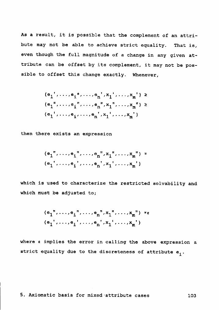
As a result, it is possible that the complement of an attri-

bute may not be able to achieve strict equality. That is,

even though the full magnitude of a change in any given at-

tribute can be offset by its complement, it may not be pos-

sible to offset this change exactly. Whenever,

(el',...,ei*,...,en',xl',...,xm') 2II II II II II(el ,...,ei ,...,en ,xl ,...,xm ) 2

I I I I(el ,...,ei,...,en ,x1 ,...,xm )

then there exists an expression

II II II II II .„,(el ,...,ei ,...,en ,xl ,...,xm ) —

I I I I I(el ,...,ei ,...,en ,x1 ,...,xm )

which is used to characterize the restricted solvability and

which must be adjusted to;

(el",...,ei",...,en",xl",...,xm") =s

(e1',...,ei',...,e¤',xl',...,xm')

where s implies the error in calling the above expression a

strict equality due to the discreteness of attribute ei.

5. Axiomatic basis for mixed·attribute cases 103

5.3.2 THEOREM

When a mixed attribute set satisfies;

1. Mutual preferential independence

2. Essentialism

3. Weak ordering

4. Archimedean property

5. Epsilon solvability,

then there exists a value function v on ei and xj fori=1,...,n and j=l,...,m such that

(el',...,en',x1',...,xm') > (e1",...,en",xl",...,xm") iff

n m n mE v(ei) + E v(x.) > Z v(ei) + 2 v(x.)

1=1 5=1 J 1=1 5=1 J

Malmborg (1981) has used epsilon solvability for the case of

binary additive. The theorem presented here is for the case

of mixed additive where discrete and continuous attributes

are considered. In the following section, we present a proof

of this theorem. The proof closely follows the line of rea-

soning used by Malmborg (1981) in his proof.

) 5. Axiomatic basis for mixed attribute cases 104

5.3.3 PROOF

Consider an attribute pair Ei, Ej. Let eg, ei* s Ei and ej,ej* s Ej where v(e*)=l, v(e°)=0, e* is the highest level and

e° is the lowest level. We also define "o" as the concat-

enation of alternatives by which level of attributes are

combined. qIf (ej*oei*) > (egoeg) and essentialism holds, then,

v(ej*) > v(e;), v(ei*) > v(e;), and thus

v(ej*) + v(ei*) > v(e3) + v(e;) = 0

‘If (ei*oe;) > (e;oej*), then we know from double cancellation

and entity independence that ei* > ej*, which implies that

v(ei*) > v(ej*).~

Furthermore, (ei*,e;) > (e;,ej*) implies

that

v(ei*) + v(e;) > v(e;) + v(ej*)

which is reduced to '

v(ei*) + 0 > 0 + v(ej*)

giving the previous result. This result can be shown for any

attribute pair Ei, Ej; i,j=l,...,n. Given that v(ei), v(ej)

are additive for any attribute pair, we can go on to prove


additivity for the entire attribute set. To do this, suppose• . • . • “

.that ei, ei s Ei, ej, ej s Ej, ea, Ga s Eij, and (ei,ej,ea)

I I I> (ei ,ej ,ea ).

It then follows that

v(ei) + v(¤j) + v(@a) > v(@i') + v(¤j') + v(ea') (1)

This is obvious if ei > ei', ej > ej', and Ea > ea', so assumethat at least one inequality is reversed. We can assume two

other possibilities;

I I Iei>ei , ej>ej , Ga >ea (2)

or

I I Iei>ei , ej >j, Ga >ea (3)

For (2), if (eioea) > (ei'oea'), then v(ei) + v(ea) > v(ei')

+ v(ea'), and from ej>ej', v(ej)>v(ej').

The result follows from combining inequalities. We, there-

fore, assume that (ei'oea') > (eioea). By epsilon

solvability, there exists a eß s Eij such that (ei'oea') =s

(eioeb) (If Eij is a continuous attribute, there exist Ea s

E.. instead of e ). As a result, °1] b


(eioejoea) > (ei'oej‘oea') =s (eioej'oeb)

so that (ejoea) > (ej'oeb), which implies;

v(<=~j) + v(ea) > v(¤j') + v(<==b) (4)

Using the result that (eioeb) =s (ei'oea'), suggests

v(ei) + v(eb) = v(ei') + v(ea'). (5)

Combining Eq. (4) and (5) gives

v(ei)+v(eb)+v(ej)+v(ea) > v(ei')+v(ea')+v(ej')+v(eb).

or

v(ei) + v(ej) + v(ea) > v(ei') + v(ej') + v(ea'). (6)

For (3), we know that, ej'>ei and ea'>ea and (eioejoea') >

(eioejoea) > (ei'oejoea') > (ei'oejoea). By epsilon

solvability, there exists ec s Ega such that

(ecoejoea') > (eioejoea) > (ei'oej'oea').

This suggests that

4 v(ei) + v(¢a) = v(@C) + v(@a') (7)

L5. Axiomatic basis for mixed attribute cases 107

and

v(ec) + v(¤j) é> =/(ei') + v(<==j') (8)

Combining Eqs. (7) and (8) yields

v(ei)+v(ea)+v(ec)+v(ej) 2 v(ec)+v(ea')+v(ei')+v(ej').

or

v(ei) + v(ej) + v(ea) 2 v(ei') + v(ej') + v(ea') (9)

By induction, these results can be extended to any partition

of the attribute set, and thus additivity for the mixed case

exists when epsilon solvability holds. QED.

5.4 MIXED MULTILINEAR CASE

The mixed multilinear case is the same as the additive case,

except·a weaker set of assumptions hold.

5.4.1 THEOREM(

For an alternative set where ei is preferentially independent

( of Ei for i=1,...,n, and xj is preferentially independent of


ij for j=1,...,m, there exists a multilinear function form

across the attribute set. Deutsch and Malmborg (1984) and

Keeney and Raiffa (1976) have considered the cases of binary

multilinear and continuous multilinear, respectively. The

case presented here is za more general case invloving mixed

multilinear. A proof of this theoren is presented next,

closely following the line of reasoning used by Deutsch and

Malmborg (1985) in their proof.

5.4.2 PROOF‘

From preferential independence, it follows that for any ei

and ei, the order of preference difference (ei',€i), (ei",€i)

depends only on the value of attribute Ei. Thus, the func-

tions v(ei',€i') and v(ei',€i") are strategically equivalent,

and as a consequence, v(ei',ei') is a linear transformation

of v(ei',Ei"). Thus,

v(ei',€i') =g(€i')

+ h(€i')v(ei',€i"), for any i. (1)

This is the property referred to by Dyer and Sarin (1979) as

conditional cardinality. If ei' = ei and Ei" = 5;, we then

have g(€i') = v(e;,€i').

Substituting this into equation (1) gives

v(ei',€i’) = v(e;,€i') + h(€°i')v(ei',.e-E-), for any i. (2)

5; Axiomatic basis for mixed attribute cases 109

Equation (2) can be rewritten as

v(e') = v(Äi') + h(€é')v(ei'), for any i. (3)

Note that v(ei') = civi(ei'), and let di(€i’) = cih(E&').

This yields:

v(e') = v(€i') + d(€i')vi(ei'). (4)

Let ei' = ei*, vi(ei*) = 1, then

(5)

Substituting (5) into (4) and rearranging,

v(e') = vi(6i')v(6i*„€i') (6)+[1—vi(ei')]v(e;,€&'), for any i

Equation (6) with i=l,

(7)

Also equation (6) with i=2,


v(e') = v2(@2')v(@2*„€2') + [1-v2(¤2')1v(e;„€2') (8)

By letting e1=e1* and el=e; in equation (8), we have

v(el*„€l')= lv2(e2')v(¢l*„e2*„€l2') (9)

andU

v(eä,€1') = [v2(e2')v(éä,e2*,El2') (10)

Substituting (9) and (10) into (7),

= v1(¤1')

+ [1-vl(el')1[v2(e2')v(eä,e2*,€12’) + [l—v2(e2')]v(éä,é;,€12')]

hn

° V(°1*·é}·E12')" V(éi·°2*·€12°)


Repeating the procedure for both discrete and continuous at-

tributes, we get the final result as followsz

n n' = 2 . . .' 2 Z Q. . .' . .'v(en

+ E E Z c.. v.(e.')v.(e.')v (e ')1:1 j>i l>j 131 1 1 3 3 1 1

+···+c123...,nwhere

ci = v(ei*,e;)

-"0 _ _cij - v(ei*,ej*,eij) ci cj

. — "•

- -

_—

-

_

cijl ° v(ei*’ej*’el*'eijl) C15 C11 cjl C1 C5 C1

cl...n= V‘C*) ° { C1...(1-1)(1+1)...¤···‘i’§>iC1j‘ { C1

The proof is therefore completed. QED.

5.5 MIXED MULTIPLICATIVE CASE

The multiplicative case is the case in which a stronger set

of assumptions than those for the multilinear case but weaker

than the additive case hold.

1


5.5.1 THEOREM

For an alternative set where el is preferentially independent

of EI, and xJ is preferentially independent of E5, for any

possible set of I,J, there exists a multiplicative function

form across the attribute set.

The cases of binary multiplicative and continuous multipli-

cative have been discussed by Deutsch and Malmborg (1984) and

Keeney and Riaffa (1976), respectively. The one presented

here is a more general mixed multiplicative case. A proof

of the mixed multiplicative theorem is presented next. The

proof closely follows the line of reasoning used by Deutsch

and Malmborg (1984) in their proof.

5.5.2 PROOF

From mutual preferential independence it follows that, for

any el and EI, the order of preference differences, (eI',€I),

(eI",EI) depends only on the values of the attributes in EI.

_ Thus, the functions v(eI',€I') and v(eI1,€I") are strate-

gically equivalent. It follows that v(eI',€I") is a linear

transformation of v(eI',€I") of the form:

v(¤I'„€I')= v(äI') + h(€I')v(eI'„€I") (1)


This is the property referred to by Dyer and Sarin (1979) as

condition cardinality. Now, let eI' = EI' and eI' = ei'.We can write (1) as

v(ei',€i') = g(ei') + h(ei')v(ei",€i'), for any i. (2)

Assume that ei" = ei, we then obtain

v(e') = g(ei') + h(ei')v(ei'), for any i, (3)

where v(€i') = v(e;,€i').

Setting all ei' = ei, except el and ej, where j-2,...,n, we

have

v(el'„¢j') = q(<·=l') + h(¤l')v(@j') (4)

= <a(¤j') + h(¤j')v(e1')„

which yield [h(e1')-1]/g(e1') = [h(ej')-1]/q(¢j'),

j=2,...,n. From this, if g(ei')=0, then h(ei')=1. It fol-

lows that

h(ei') = X g(ei') + 1, for any i (6)

We can repeatedly use equation (3) to obtain


(7)h(e1') ... h(e'¤_1)g(en').

Substitutinq (6) into (7) yields

v(e') = q(¢1') + lXq(¤1') + 11 q(e2‘) + --- +{[xg(el') + 1] [)(g(e'¤_l) + 1]}q(en')

n j-1( = q(e1') + Z H lkq(@i') + 11q(e-') (8)5=2 1=1 J

We then multiply both sides of (8) by k, and add 1 to each

side,

n j·1Xv(e') + 1 = Xg(e1') + 1 + 2 H [Xg(ei') + 1]g(ei')X

j=2 i=1

nXv(e') + 1 = H [Xg(ei') + 1] (9)

i=1

and g(ei') = civi(ei').

This completes the proof. QED.·

5.6 MIXED ADDITIVE INTERDEPENDENT CASE

The result is this section deals with the additive form whenattributes have overlapping dependencies.


5.6.1 THEOREM

Let N={1,...,S,S+1,...,n}, where (n23), denote a

unidimensional attribute set where i=1,...,S are discrete

attributes and i=S+1,...,n are continuous attributes. Sup-

pose N is decomposed into the overlapping partition,

Y1,...,Ym, where, (n>m23), and this m-component partition

satisfies the following: -

1. Mutual preferential independence among partitions

2. Essentialism

3. Weak ordering

4. Archimedean property

5. Epsilon solvability

Then, for all e ,e' s E, there exist real valued functions

v(Y1),...,v(Ym), such that

m me > e' ==> v(e) = Z v(Yi) > v(e') = E v(Yi'),

i=1 i=1 _

where ‘A

v(Y1) = f(Yl)

and

i-1 kv(Yi) = f(Yi) + x (-1) 2 f(Yi¢\...0Yi ).k=1 1si,<...<ik<i 1 k

¥5. Axiomatic basis for mixed attribute cases 116

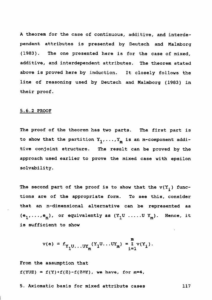
A theorem for the case of continuous, additive, and interde-

pendent attributes is presented by Deutsch and Malmborg

(1983). The one presented here is for the case of mixed,

additive, and interdependent attributes. The theorem stated

above is proved here by induction. It closely follows the

line of reasoning used by Deutsch and Malmborg (1983) in

their proof.

5.6.2 PROOF

The proof of the theorem has two parts. The first part is

to show that the partition Y1,...,Ym is an m-component addi-

tive conjoint structure. The result can be proved by the

approach used earlier to prove the mixed case with epsilon

solvability.

The second part of the proof is to show that the v(Yi) func-

tions are of the appropriate fomm. To see this, consider

that an n—dimensional alternative can be represented as

(el,...,e¤), or equivalently as (Y1U .....U Ym). Hence, it

is sufficient to show

mv(e) = fY U(((UY (Y1U...UYm) =(E v(Yi).

1 m 1-1

From the.assumption that (

f(YUZ) = f(Y)+f(Z)-f(ZhY), we have, for m=4,


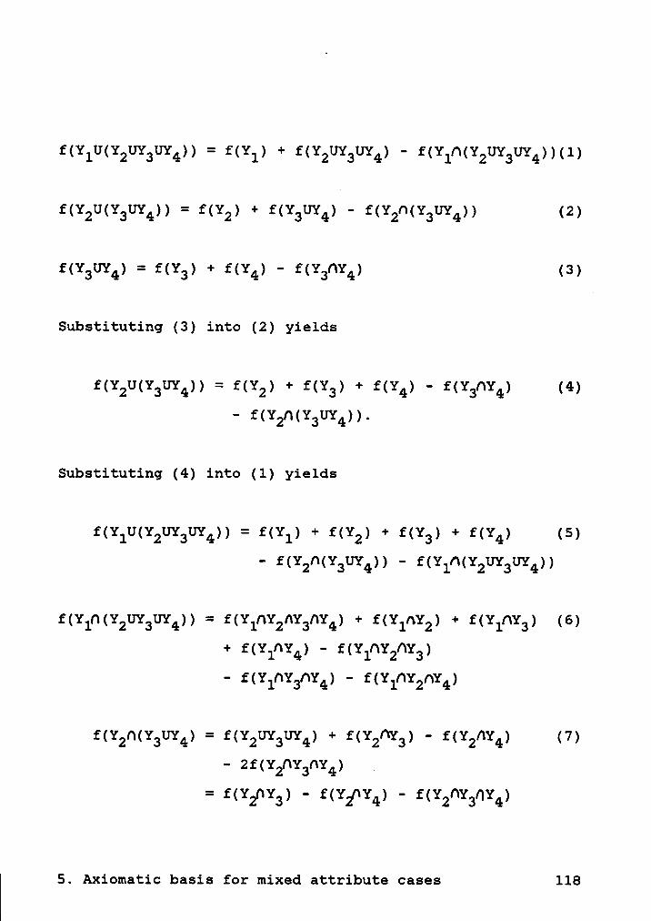
f(Y1U(Y2UY3UY4)) = f(Y1) + f(Y2UY3UY4) - f(Y1A(Y2UY3UY4))(1)

f(Y2U(Y3UY4)) = f(Y2) + f(Y3UY4) - f(Y2¤(Y3UY4)) (2)

f(Y3UY4) = f(Y3) + f(Y4) — f(Y30Y4) (3)

Substituting (3) into (2) yields

f(Y2U(Y3UY4)) = f(Y2) + f(Y3) + f(Y4) - f(Y3hY4) (4)

- f(Y2h(Y3UY4)).

Substituting (4) into (1) yields

f(Y1U(Y2UY3UY4)) = f(Y1) + f(Y2) + f(Y3) + f(Y4) (5)

— f(Y2h(Y3UY4)) — f(Y1^(Y2UY3UY4))

f(Yf¤(Y2UY3UY4)) = f(Y1nY2AY3hY4) + f(Y1nY2) + f(Y1AY3) (6)

+ f(Y1^Y4) - f(YIHY2^Y3)

- f(Y1/WY3/WY4) - f(Y1f\Y2hY4)

f(Y2h(Y3UY4) = f(Y2UY3UY4) + f(Y2^Y3) - f(Y2hY4) (7)

- 2f(Y2HY3hY4)

= f(Y20Y3) — f(Y20Y4) - f(Y2^Y3OY4)


Substituting (6) and (7) into (5),

f(YlUY2UY3UY4) = f(Yl) + f(Y2) + f(Y3) + f(Y4)

- f(Y1(\Y2) - f(Ylf\Y3) - f(Y1/'\Y4)

- f(Y2f\Y3) · f(Y2f\Y4) - f(Y3f\Y4)

+ f(Ylf\Y2f\Y3) + f(Y1(\Y3('\Y4)

+ f(Y1f\Y2f\Y4) + f(Y2{\Y3{'\Y4_)

- f(Y1f'\Y2t\Y3GY4)

4= 2 f(Yi) - Z f(YiGYi )i=l l$i\ <i1 1 2

+ Z f(YiGYiÜYi )1si„<i1<i3 1 2 3

- f(Y1f\Y2/\Y3ÜY4).

By induction, we can show that, for any m,

f(Y1U...UYm)

=I;

f(Y ) - E f(Y GY ) (-1)m-lf(Y"(': GY)1=1 1 1<i( <1, 11 12 ‘“

Since v(Y1) = f(Yl), and

i—1 kv(Yi) = f(Yi) + Z (-1) E f(Yi (\...{\Yi ),k=1 1si,<...<ik<i 1 k

1 then


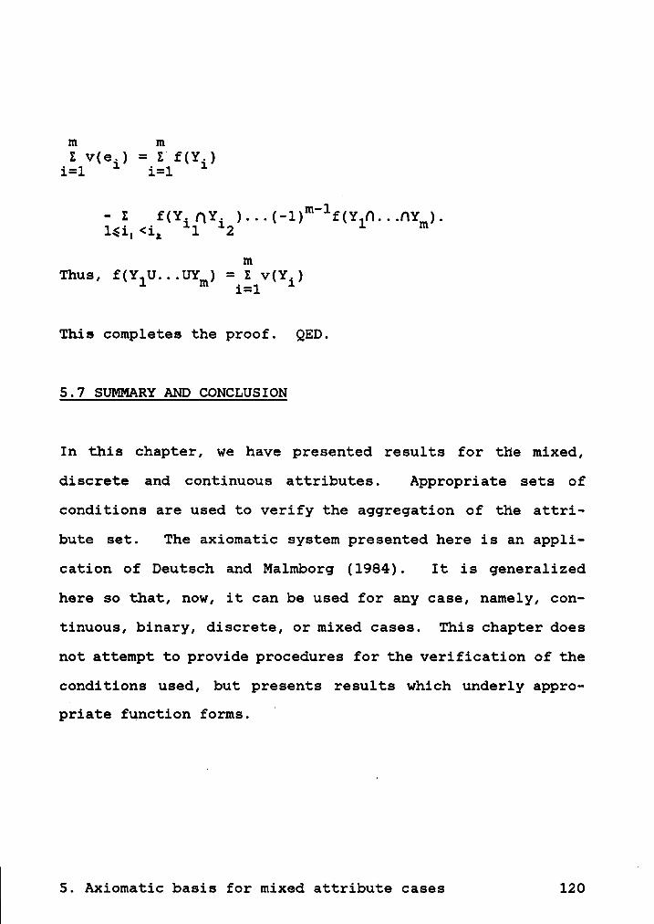
m mZ v(e.) = Z f(Y.)

1=1 1 1=1 1

m-11- 2 f(Yi{\Yi )...(-1) f(Y1O...0Ym).161, <1, 1 2

mThus, f(Y1U...UYm) =·E v(Yi)

1-1

This completes the proof. QED.

5.7 SUMMARY AND CONCLUSION

In this chapter, we have presented results for the mixed,

discrete and continuous attributes. Appropriate sets of

conditions are used to verify the aggregation of the attri-

bute set. The axiomatic system presented here is an appli-

cation of Deutsch and Malmborg (1984). It is generalized

here so that, now, it can be used for any case, namely, con-

tinuous, binary, discrete, or mixed cases. This chapter does

not attempt to provide procedures for the verification of the

conditions used, but presents results which underly appro-

priate function forms.1


6. METHODOLOGY FOR CREATING LAYOUT ALTERNATIVES

In this chapter the methodology of using closeness preference

ratings to determine relative department locations is de-

scribed. First, the layout design problem is formulated as

a quadratic assignment problem and some solution procedures

suggested ixx the literature for solving the quadratic as-

signment problem are reviewed. Then, a heuristic procedure

based on the solution of a small size quadratic assignment

problem is described to obtain an initial layout which gives

locations of various departments. This initial layout is

used as a guideline to obtain the final layout by taking into

consideration the actual department sizes. The process of

constructing the final layout is also described. An example

problem is presented to demonstrate the proposed procedure.

CORELAP and ALDEP are also applied to the same problem and

the results obtained from all three procedures are compared.

A detailed comparison between the results obtainmd using

CORELAP and the proposed procedure is then presented. The

proposed procedure is shown to consistently give better lay-

outs than those obtained using CORELAR.

,6. Methodology for creating layout alternatives 121

6.1 LAYOUT DESIGN AS A QUADRATIC ASSIGNMENT PROBLEM

In the previous chapter we described a methodology of meas-

uring accurate closeness ratings. Now, we develop a proce-

dure for layout construction based on the objective of

maximizing closeness ratings. The problem of determining an

optimal layout can be formulated as a quadratic assignment

problem (QAP) as follows:

n n n nMax Z E E Z c.. x..x

1=1 5=1 k=1 1=1 1JkJ JJ kl

Subject to

nE xi.= 1 j=l,...,n

1=1 J

n2 xi.= 1 i=l,...,n

i=l J

where

xij = 1, when department i is assigned to location j

= O, otherwise

n = total number of departments

pik = closeness rating between departments i and k

djl = rectilinear distance between locations j and 1

. and ·

t

6. Methodology for creating layout alternatives 122

cijkl = pik/djl. The symbol, cijkl, represents the close-

ness rating between a department pair i,k, depending upon the

rectilinear distance between the locations that they are as-

signed to. The greater the distance between departments, the

smaller is the closeness rating between them.

In the above formulation, the objective function represents

total closeness rating between departments. The first con-

straint ensures that only a single department is assigned to

a location and the second constraint ensures that a depart-

ment is assigned to only one location. This formulation as-

sumes that the departments are of the same size. In case the

departments are of different sizes, the above formulation

becomes

n m n mMax Z E 2 Z c., x..x

1=1 5=1 k=1 1=1 1Jkl lJ kl

Subject to

nZ xij= si i=l,...,n

i=1

2 xi.= 1 j=1,...,n1=1 J

where,



= O, otherwise

si = number of blocks for department i

m = total number of blocks

and

cijkl = pik/(djlsisk) = closeness rating between a depart-

ment pair i,k.

6.2 LITERATURE REVIEW OF PROCEDURES TO SOLVE THE QAP

Generally, the quadratic assignment problem (QAP) seeks to

assign I1 departments to I1 mutually exclusive locations, so

as to minimize the total quadratic interaction term. In our

case, the objective is that of maximization. The QAP was

first formulated when Koopmans and Beckmann (1957) studied

problems concerning the allocation of plants to sites. Sub-

sequently, considerable work has been done by mathematicians

and engineers alike on problems of a similar nature. How-

ever, the problem still remains of considerable interest due

to the variety of possible solution approaches and the number

of applications it has in various fields.

The nonlinearity and combinatorial nature of the problem

creates difficulties in developing efficient solution tech-

niques. The number of possible permutations for the problem

grows exponentially with an increment in the value of n.i

Exhaustive enumeration for even a modest size problem is

i


computationally infeasible. For example, Nugent, et. al.

(1968) estimate that for n=12 (for which n!=4.79*l0) the

total enumeration on an IBM 7090 computer would require three

years of cpu time.

Solution methodologies for the QAP can be classified under

two categories, namely, exact and heuristic methods. Exact

methods are those which determine the optimal QAP solution.

Heuristic methods generally determine a suboptimal solution.

6.2.1 EXACT METHODS EMPLOYING BRANCH AND BOUND

These are exact procedures for assigning n departments to n

locations by enumerating, in a controlled manner, all the

possible location—department permutations. Many of the per-

mutations are handled implicitly, thus reducing computational

effort.

The general method employed is as follows. Starting from

node zero at which no department is fixed, branches are cre-

ated, mo systematically partition the solution space. Each.

branch represents the allocation of a department to a lo-

cation or vice versa and it terminates in a node. A node in

the enumeration tree represents a subproblem at which the

solution is restricted to satisfy the conditions imposed on

the branches connecting it to node zero. Thus, a path from


node zero to the bottom of the tree prescribes allocation of

departments to locations. Once a department or a location

is assigned to any particular node it is labelled. The un-

assigned departments or locations are label free. Creating

branches until all the departments are fixed to all possible

locations, is equivalent ‘¤oenumerating all the location-

department permutations. However, this is avoided by com-

puting lower bounds (upper bound for the maximization

problem). This is defined as follows. The lower bound (Up-

per bound) at any partial placement (corresponding to a node)

is a value which indicates that every possible combination

of the free departments will yield an objective value higher

(lower) than this value in case of the minimization

(maximization) problem.

The lower bound (upper bound) at any partial placement can

be broken down into three components:

1. A value bl which gives the interaction cost (closenessu

rating) between the assigned department themselves.

2. A value bz which a lower bound (upper bound) on the

interaction between the assigned departments and the un-

assigned departments.

i


3. A value b3 which is a lower bound (upper bound) on the

interaction between the unassigned departments them-

selves.

Thus, if the objective function value of some known feasible

complete placement is lower (higher) than the lower bound

(upper bound) of a partial placement, then the node corre-

sponding to this partial placement, and its descendants, can

be eliminated from further consideration. This process of

eliminating further branches from a node is termed fathoming

the node. The best known objective function value of a com-

plete placement is referred to as the upper bound (lower

bound) or the incumbent value. This underlies the importance

g of lower bounds i11 a branch and bound procedure. Better

lower bounds (upper bounds) fathom a greater portion of the

enumeration tree thereby reducing the computational effort.

The various exact methods employing branch and bound pre-

sented in the literature differ primarily in the methods used

for branching and for the computations of bounds. Next, we

briefly describe these methods.

A class of methods proposed for QAP is termed single assign-

ment algorithms. All algorithms in this class deal with as-

signing a particular department to a location at each node.

The algorithms vary primarily in the method of computing the

lower bound, and the branching procedure.

i

6; Methodology for creating layout alternatives 127

Gilmore (1962) presented an algorithm which is a semi-

enumerative one. The algorithm associates a particular lo-

cation or department to each level in the branching process.

For each location, the distances from all other locations are

computed and they are arranged in a non-increasing order.

The departments/locations are then assigned to each level in

this order. The algorithm starts from the top of the tree

assuming an initial solution. Search is performed using the

depth first strategy. Branches are fathomed when lower

bounds are found to be greater than the incumbent solution.

The lower bounds are calculated by the previously described

method. The search backtracks to the next higher level and

resumes. The efficiency of the algorithm depends largely

upon the initial solution. The algorithm is not computa-

tionally feasible for n larger than 15.

Lawler (1963) presented a technique to calculate the lower

bound of the cost function based on xeplacing the binary

variable xij= 0 or 1 by xijz 0. The resulting problem is then

solved by a quadratic programming technique. The branching

process is the same as Gilmore's.

Graves and Whinston (1970) identified the statistical prop-

erties of the cost function. They used these statistical

properties in conjunction with a general enumerative proce-

dure to define a solution algorithm. Using the idea of con-

f


fidence level enumeration, this algorithm allows for an

effective treatment of QAP. The branching process is bas-

ically the same as Gilmore's.

Unlike the single assignment algorithms, pair assignment al-

gorithms assign pairs of departments, i and j, to locations

k and p. Land (1963), Gavett and Plyter (1966), and Pierce

and Crawston (1971) have developed algorithms in this regard.

For the case of 11 departments and n locations, there are

n(n-1)/2 pairs of departments and n(n-1)/2 pairs of lo-

cations. Thus, given four departments A, B, C and D, and four

locations 1, 2, 3 and 4, there are the following possible

pairs of departments and locations:

Department pairs: (A,B) (A,C) (A,D) (B,C) (B,D) (C,D)·

°

Location pairs: (1,2) (1,3) (1,4) (2,3) (2,4) (3,4)

A feasible assignment of these pairs does not necessarily

provide a feasible solution to the original problem. To il-

lustrate this, suppose department pair (A,B) is assigned to

location pair (1,2) and the department pair (A,C) is as-

signed to location pair (3,4). This is not a feasible sol-

ution since .department A is assigned to two locations.

Hence, additional constraints are introduced in the linear

pair assignment problem so that a solution to this linear °

assignment problem gives a feasible solution to the original

problem. —The solution technique proceeds level by level by

fixing a new pair of departments to a pair of locations.

i


Land (1963) used a simple assignment matrix to establish the

cost lower bounds on the branches of the tree. However, the

method involved enumeration of the set of n! feasible sol-

utions, a task which becomes impossible even for moderate

values of n. Gavett and Plyter (1966) also used simple as-

signment matrix but instead of employing only* a column-

reduced matrix, they used a row and column-reduced matrix to

establish the lower bounds. Both algorithms proceed level

by level in the search tree, committing one new pair to the

solution at each level, and backtracking to the next higher

level in the search tree. Pierce and Crawston (1971) intro-

duced the pair-exclusive algorithm method. This method

'eliminates some of the feasible solutions at each stage of

the stepwise process. The solution procedure uses a tech-

nique similar to that of the pair assignment algorithm to

determine pair assignments. If the relaxed problem of as-

signing pairs produces an infeasible assignment, then some

conflicting assignments exist which should not be part of the

optimal solution. The search tree then branches into as many

nodes as there are conflicting assignments, removing* one

conflicting assignment at each node created. Having

branched, lower bounds are computed at each descendent node.

For this purpose, an assignment problem with the additional

pair exclusion constraints is solved at each node. If this

does not result iax a feasible solution, and if the lower

bound does not exceed the upper bound at any node, then fur-

\


ther branching is necessary. However, if a feasible solution

is obtained, then that node is fathomed. At any stage, the

procedure selects another node with the lowest bound and

proceeds as before. When all nodes are fathomed the algo-

rithm terminates. „

The branch and bound methods have been found to be computa-

tionally feasible only for problems of size twelve or less

number of departments. Consequently, other methods have also

been developed which we discuss next.l

6.2.2 EXACT METHODS NOT EMPLOYING BRANCH AND BOUND

These approaches use techniques such as integer programming,

quadratic integer programming, cutting plane algorithms and

decomposition principles to solve the QAP.

First, Cabot and Francis (1970) showed that for the QAP with

linear constraints, the optimal solution is the extreme point

of the convex set of feasible solutions. They presented a

procedure for solving such a problem. Their methodology in-

volved first determining a related linear program containing

the original set of constraints. The extreme-point-ranking

approach of Murty (1968) was then applied to this linear

program to obtain an optimum solution to the QAP.

{


Love and Wong (1976) formulated the QAP as a binary mixed

integer program. This formulation is as follows.

n nMin

iil jélwij(Rij+Lij+Aij+Bij)

Subject to

Rij-Lij = xi- xj 1=1,...,n-1A..-B.. = .- . '=' 1 .11 11 Y1 Y1 J 1+

nxi + yi =

kilskaik i=l,...,n

nxi — yi = kil

dkaik i=1,...,n

nE a. = 1 i=1,...,n

k=1 lk

n·E aik = 1 k=1,...,n1-1

where aik= 1 when department i is assigned to location k

= 0, otherwise

n = number of departments

wij = flow (interaction) between i and j

Rij = horizontal distance between departments i and j

if i is to the right of j, and is zero otherwise


Lij = horizontal distance between departments i and j

if i is to the left of j, and is zero otherwise

Aij = vertical distance between departments i and j

if i is to above of j, and is zero otherwise

Bij = vertical distance between departments i and j

if i is to below of j, and is zero otherwise

(xi,yi) = location of department i, i=1,...,n

sk = sum of coordinates of location kdk = difference of coordinates of location k

The first four constraint types guarantee that none of the

departments are overlapped. The last two constraint types

ensure that one department must be assigned to only one lo-

cation. This formulation has nz binary variables and (n2+3n)

constraints. It can be solved using integer programming

codes. However, it is restricted to relatively small prob-

lems (ns9) due to the number of constraints. It has the ad-

vantage of not requiring quadratic assignment code.

Another well known method used for solving QAP involves the

construction of an equivalent, but much larger linear as-

signment problem with several side constraints. The drawback

of this method lies in the weakness of the bounds obtained

by solving the linear problem. Kaufman and Broechx (1978)

suggest an alternate linearization using Glover’s

}


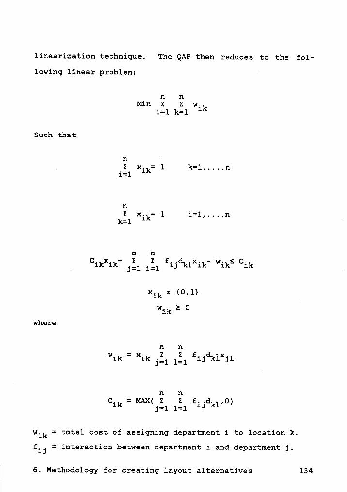
linearization technique. The QAP then reduces to the fol-

lowing linear problem: ·

n nMin Z Z w.

1=1 k=1 lk

Such that

~

.ill

xik= 1 k=l,...,n

n

kilxik=1n

nC1kk1k+ jil iil fijdklxik- wiks Cik g

xik s {0,1}

wik 2 0where

n n. = . Z E f..d · .wik xik j:1 1:1 13 klxjl

n nC. = MAX( E Z f..d ,0)1k j:l 1:1 ij kl

wik = total cost of assigning department i to location k.

fij = interaction between department i and department j.


dkl = distance between location k and location 1.

xik = l, department i is assigned to location j

= 0, otherwise.

The third constraint of the formulation ensures that any as-

‘signment of department i to location k results in minimum of

total cost.

Glover's method introduces n new continuous variables and n

new constraints. The problem can be solved using a code for

mixed integer programming. Furthermore, solution method is

suggested for the linearized QAP which is based on Bender's

decomposition.

Bazaraa and Sherali (1980) consider a formulation similar to

that of Kaufman and Broeckz (1978). They applied Bender's

partitioning scheme to solve the model. This approach de-

composes the model into a linear integer master problem and

a linear subproblem. At each iteration, the master problem

generates a point XA, based on which a suitable subproblem

is solved to generate a cut-constraint. This cut is then

appended to the other constraints in the master problem and

the solution to the latter is updated. The procedure hence

alternates between the master problem and the subproblem un-

til a suitable termination criterion is met in a finite num-

ber of steps. (

i


6.2.3 HEURISTIC METHODS

A heuristic method is a common sense approach to provide ap-

proximate solutions to problems. They remain the only ef-

fective methods of solving large sized problems which exist

in reality. A heuristic, however, is not an exact approach

and it is usually not possible to guarantee or verify opti-

mality. Typically, solutions are closely sub-optimal.

The heuristics for QAP existing in the literature can be

classified as follows.

1. Construction procedures - These methods select departments

to be placed on locations one-at-a-time sequentially. This

continues until all departments have been located using cer-

tain rules. One method in this regard suggested by Rajgopal

(1985) is summarized below.

Let (D,L) be a partial assignment where L represents a set

of locations and D(L) represents the departments that are

assigned to the locations in set L. Let

A. = 2 (d. +d .)1 p not: L lp pl

lB. = 2 (p. +p .)l qnots D(L) lg gl


where dip = distance between locations i and p

pjq = interaction between department j and q

Then assign an index i with minimal value Ai to an index j

with maximal value Bj. The procedure is repeated until all

departments have been assigned.

2. Improvement procedures - These methods start with a fea-

sible arrangement of departments to locations, and then sys-

tematically improve that solution. A method in this regard

is to perform a pairwise interchange between departments.

Hillier (1963) used this method for QAPs with the grid

structure. According to this method the maximum movement of

a department either, left, up or down is first determined.

This is termed the maximum number of steps, p. The p step

movements of all the departments is considered and the cost

of all these p step movements to their corresponding sites

is determined without the counter movement of the department

occupying the site. The interchange of departments is con-

sidered with the department that offers the maximum cost re-

duction. The interchange is implemented only if it results

in a decreased cost. The move numbers are then updated and

the procedure continues until no more p step improvements are

possible. Next p is decreased by one and the process is re-

peated. q This procedure was further improved by Hillier and

Connors (1966) by considering in the preliminary moves only

}


those improvements which decreased the cost by at least a

specified amount.

Armour, Buffa and Vollman (1963) developed the well known

method of CRAFT. From an arbitrary starting solution, they

computed the decrease in cost by interchanging each pair of

departments. Only those pair interchanges that resulted in

the minimum cost were implemented. This method terminates

when no more improvement is possible.

Vollman, Nugent, and Zartler (1966) suggested the following

two phase technique which was a considerable improvement over

CRAFT. In the first phase, the two facilities which con-

tributed most to the cost were selected. All pairwise

interchanges with one of the chosen departments were computed

and the largest reduction was implemented. The department

interchanged was then disregarded from further consideration.

When no further improvements were possible with the first·

department chosen, the procedure was repeated with the second

department. Again two departments with the greatest con-

tributions to cost were chosen and the process was repeated.

This continued until no further improvements resulted. The

procedure then switched over to the second phase, where all

possible pairwise interchanges were attempted. The entire

procedure was repeated once more and then terminated.

, 6. Methodology for creating layout alternatives 138

Pagels (1966) used a discrete optimization technique adopted

by Reiter and Sherman (1965) to develop a heuristic. All

possible pairwise interchanges were done on a random layout

giving a local (2—opt) minimum. This was used to generate a

second starting layout giving a second local (2-opt) minimum.

The user was then asked to provide a value for the probabil-

ity of not finding the optimal solution at termination, this

was then used to determine the number of iterations to be

performed.

Los (1978) proposed the following technique to improve upon

CRAFT. All possible exchanges were evaluated only once. At

each exchange the computed exchange values were updated

recursively, thus reducing the computational effort for all

subsequent iterations.

Patel, Dewald, and Cote (1976) used the following concept to

reduce computational effort. They created algorithms to

partition the departments into groups of departments in such

a way that the interactions between the groups was minimized.

It was desirable to have an equal number of departments in

each group. Highly interconnected departments were put to-

gether and referred as groups or supernodes. This was done

until the required number of supernodes were formed. The

locations were then divided into superlocations and super-

nodes were allotted to superlocations and improved by

}6. Methodology for creating layout alternatives 139

pairwise interchange. After this placement, pairwise inter-

change was conducted within the elements of each supernode

only, thus reducing the computational effort considerably.

Other improvement schemes are more complex than the pairwise

interchange technique described before. They are the combi-

nations of several other methods. For example, Burkard and

Stratman (1978) alternated between a branch and bound ap-

proach and an improvement exchange routine. Bazaraa and

Sherali (1980,1982) implemented Benders partitioning method,

and a disjunctive cutting plane method on a mixed integer

formulation of the QAP. The details of some of these proce-

dures are discussed next.

The heuristic of Gaschutz and Ahren's (1968) imbeds the

problem into a graph theoretic framework in which the nodes

represent the departments. In this graph, departments with

a positive interaction are connected by links having weights

proportional to the level of interaction. A continuous re-

laxation technique is then employed to determine coordinates

of the nodes such that the sum of weighted square deviations

of the nodes from each other is minimized. This is subject

to a normalization constraint that the sum of the x and the

sum of the y coordinates should each equal zero, and the sum

of their squares should each equal unity.· An iterative

scheme is used to solve this problem. The resulting coordi-


nates are then used to match the departments onto the lo-

cation grid.

Burkard and Stratmann (1978) alternated between a branch and

bound approach and an improvement exchange routine. Their

method called VERBES, terminate when no further improvement

is possible. This method yielded very good results.

Bazaraa and Sherali (1980,1982) were able to obtain solutions

of equivalent and better quality than those obtained by

Burkard and Stratmann (1978) for the test problems. They

implemented Benders partitioning method, and a disjunctive

cutting plane method on a mixed integer formulation of the

QAP. They empirically demonstrated the prohibitiveness of

using these methods as exact algorithms, and developed the-

oretical lower bounds on computational complexity in some

cases. They then converted these algorithms to heuristic

procedures which were able to produce better quality sol-

utions on test problems than any of the previous methods.

Mirchandani and Obata (1979) also employed Gaschutz and

Ahrens (1968) method along with Hall's (1970) algorithm for

solving the squared deviation problem as a preprocessor in a

rotating grid algorithm. In their method, several trial

solutions were obtained by attempting to match the locations

of the placement-grid as it rotated into several positions

i


superimposed upon Gaschutz and Ahrens' solution. Thisr

matching was performed by using an assignment problem to ob-

tain a least deviation from the Gaschutz and Ahrens' sol-

ution. A pairwise exchange was then performed over each

resulting solution. In addition, the mixed-exchange scheme

discussed earlier was used to improve the solution.

Rajgopal (1985) divided the problem of n

departments/locations into several subproblem of size less

than six departments/locations. Each subproblem was then

solved using a branch and bound method. Later, a pairwise

interchange routine is performed on the overall problem. The

method is a polynomial time heuristic with respect to the

size of the problem.

6.3 A SOLUTION PROCEDURE FOR THE DETERMINATION OF THE INITIAL

LAYOUT

In this section we develop a new heuristic solution procedure

for the layout problem formulated as a QAP. Most of the exact

algorithms presented so far in the literature, for the sol-

ution of QAP, do well for small problems. These procedures

require substantial computer programming memory and computer

running time for a realistic size problem. In contrast,

heuristic methods require less computer memory and computa-

tion time. The principal aim of the heuristic developed here

>


is to provide a good solution in a reasonable amount of time

when run on a personal computer system.

The proposed heuristic is of a construction type and can be

coupled with either a pairwise interchange routine or another

improvement routine described below to improve solution

quality. The following construction routines can be used to

build a starting solution which can subsequently be subjected

to improvement.

Construction routine 1:

Let (D,L) represent a partial assignment where L represents

a locations set and D(L) represents the departments set which

are assigned to the locations set L. Let

A. = E (d. +d .)1 p not: L lp pl

B. = Z (p. +p .)J qnot: 1>(L.) Jq qJ

where i Q L, j Q D(L). Assign location i with minimal value

Ai to department j with maximal value Bj. Then replace L by

L U {i} and compute new values of Ai and Bj. The process

continues until all departments have been assigned ‘¤o lo-

cations. This routine is similar to that suggested by

Rajgopal (1985) and described in section 6.2.3 except that

t


the sets Ai and Bj are updated here whenever a department is

assigned to a location.


Let k represent the order of department/location to be in-

troduced into the layout. The first step is performed as in

construction routine 1 to find the first assignment. Let

k=l. If an il was assigned to a jl, then, at the next step,

assign an i with minimal(dii +di i) to a j with‘1 1

maxima1(p.. +p. .). Set k=k+l. Then, i and j are replaced111 111 1 1by ik and jk and the process continues until all departments

have been assigned to locations.


Let (D,L) represent a partial assignment where L and D are

as defined earlier. Also determine Ai and Bj as before. Thatis,

A. = Z (d. +d .)1 p not: L lp pl '

B- = Z (p- +p -),J q mc: 11(L) Jq Q1

where 1. s L, j s D(L). Rank Ai in the increasing order of

its values. Assign location i with minimal value_Ai to de-partment j with maximal value Bj . Make L = L U {i} and update

Ä


D(L). Select the next higher Ai value from the ordered list

and assign a department j s {l,...,n}-D(L) to this i such

that

PELpi /dip

is maximal. Denote the department j which is assigned to

location i by D(i). The process repeats until all

departments/locations have been assigned.

j These three construction algorithms are used to create ini-

tial layouts. Each of them is designed to accommodate vari-

ous types of preference matrices. Construction algorithm l

gives better solutions when the positive entries in the

preference matrix are not much different from each other, as

this method considers aggregate rating of a department with

others. Construction algorithm 2 gives better solutions when

only a few departments are dominating and have large values

of the corresponding entries in the preference matrix, since

it searches for a department pair with the highest preference

value among those available and puts those departments next

to each other. In the case where several entries in the

preference matrix are sufficiently larger than the others,

construction algorithm 3 gives better solutions, since it

selects a department to enter the layout which maximizes the

total preference value of the layout obtained so far.

}


Improvement routine:

The improvement routine suggested here is designed to produce

a good solution in a reasonable amount of time. Since the

routine is implemented on a microcomputer system, the com-

puter memory and computation speed are two major concerns.

The improvement routine is a blend of solving a subproblem

using the exact method and alternating it with a pairwise

interchange routine described below. The size of the sub-

problem for the exact method is arbitrarily chosen here to

be 5, due to the concerns of computation time and computer

memory for larger subproblem size. The details of the im-

provement routine are described next.

Let Ld be an ordered list of locations corresponding to the

values of Ai and n be the number of locations under consid-eration (which is also equal to the number of departments).

1. Initialize S=Ld, nS=n and denote by f(i) the facility

which is currently fixed on location site i, i=1,...,n.

2. Let nd=min{ng,5} and denote by Sd the top nd locations

in S. Accordingly, define Sf= {p:p=f(i) for i s Sd}.

Solve for an exact solution of QAP(Sf,Sd). Update f(i),

i s Sd. The QAP is solved here using exhaustive search

as the subproblem size is relatively small, namely 5.

i


In case a larger subproblem size is selected, the QAP can

be solved by a more effective method.

3. Set nS=nS—k. That is, consider the next subproblem from

among the nS—k locations where the assignment of depart-

ments to the first k locations is fixed. A large value

of k will give relatively small overlap among the sub-

problems, while a small value of k will result in rela-

tively large computation time. A value of k=2 was found

to be a good compromise. If n $4, then stop. Otherwise,

remove the top two locations from S and go to step (2).

The solution obtained above can further be improved using a

pairwise interchange routine described in the following sec-

tion.

Pairwise interchange routine:

Let f(i)=j for i=1,...,n and j=1,...,n as an initial sol-

ution, where f(i)=j represents facility j being assigned to

location i.

1. Let il,i2 represent a location pair.

2. Set il=1, i2=2. Calculate total preference. Let k=i2.

i


3. Interchange locations of facilities f(i1) and f(i2).

Calculate total preference. If the new total preference

is greater than the previous one, the interchange is

successful. Otherwise, go to the next step.

4. If i1=n—1, i2=n, then terminate the process.

5. If i2=n, then go to step (6). Otherwise, i2=i2+1, and

go to step (3).

6. Set i1=i1+1, i2=k+1, k=i2 and go to step (3).

•Implementation of the Proposed Procedure to the Case of Une-

gpal Department Size:

Next, we discuss the application of the above procedure to

the case of unequal department sizes. As was discussed ear-

lier in section 6.1, unequal departments can be represented

as several blocks of a basic unit size. If the above

heuristic method is directly applied to the blocks corre-

sponding to each department, it is possible that the final

solution may give-an infeasible solution. That is, blocks

of the same department may not be adjacent. In order to force

the blocks of the same department to be adjacent, a penalty

function concept can be applied. That is, a very large value

of. cijkl is added in the objective function as a penalty

i~6. Methodology for creating layout alternatives 148

among blocks of the same department, to force them to be ad-

jacent. Consequently, the formulation is as follows:

n m n mMax 2 2 Z Z c.. x..x

1=1 5=1 k=1 1=1 13k1 13 kl

Such that

mZ xij= si i=1,...,n

i=1

n

ill xij= 1 3=1,...,m

where


= O, otherwise

and

cijkl = pik /(djlsisk) = closeness rating for the depart-

ment pair i,k; this is a function of preference rating and

rectilinear distance of relative locations; cijkl = M (a

very large value), when i=k.

pik = closeness rating between departments i and k

djl = rectilinear distance between locations j and 1 „

si = number of blocks for department i

m = number of total blocks

n = number of departments

i


By selecting an appropriate value of M, the proposed method

can be applied effectively. A modification needs to be made

in the implementation of the proposed method. In the pro-

posed method, a set of five locations and their corresponding

departments are chosen and are rearranged by solving the QAP.

In the case of departments of unequal sizes, it is possible

that only a subset of blocks belonging to a department are

contained in the selected set of five locations. Conse-

quently, in the improvement routine, the subset of blocks of

a department, that are contained in the selected set, will

not move from their current locations due to a large value

of closeness rating, cijkl, between them and their counter-parts outside the selected set. A modification is therefore

made in the algorithm to either include or exclude blocks of

the same department in the selected set. A step by step

strategy for the selection of the location set is as follows.

Step 1: Set n=l.

Step 2: The nth location in the set is chosen as described

in the improvement routine.

Step 3: Check whether more than one block is required for the

department in the nth location. If so, go to step 4. Oth-

erwise, set n=n+l and repeat step 3 until the location set

is filled.

}


Step 4: Assume that the department selected requires m

blocks. If m is greater than the number of locations remain-

ing in the location set, go to step 2 and select the next

location on the ordered list as described in the improvement

routine; otherwise, go to step 5.

Step 5: Assign the locations corresponding to the selected

department to the location set. Set n=n+m, then go to step

2.

By applying the above strategy, we can assure that, when the

QAP is solved, all blocks are free to move. This yields a

better solution than obtained by directly applying the pro-

posed routine to the case of unequal size departments.

6.4 A PROCEDURE FOR DETERMINING THE FINAL LAYOUT

The layout determined by the method of section 6.3 is termed

an initial layout or blockplan because it only gives lo-

cations of various departments. From this we need to con-

struct the final layout, taking into consideration the actual

department sizes. A procedure to do that is as follows.


Step l: Take the department from the first location of row

one in the blockplan and locate it in the upper left hand

corner of the actual layout plan. Take the department from

the second location of row one in the blockplan and place it

next to the previously located department. The same process

continues until departments in the first row of the blockplan

are all placed. If it occurs that departments cannot fit in

the layout, go to step 2, otherwise, continue the same proc-

ess for row two, and so on until all departments are placed

in the final layout or a department cannot fit in the layout.

In which case, go to step 2.

Step 2: Check whether an acceptable adjustment in the shape

of the department can be made so that the department can now

fit in the layout. If so, alternate the department shape and

rearrange it and go back to step 1; otherwise, go to step 3.

Step 3: Either remove the first or the last department of

the row in consideration and rearrange the rest of the de-

partments in that row to fit in the layout. Place the first

or the last department (whichever selected) below the secondu

or the second last department, respectively. If it is fea-

sible to do so, then continue with step 1 in the next row;

otherwise, discard the blockplan and try other blockplans.


X

These steps provide a general guideline to convert an initial

layout into a final layout. However, some layout problems

involve departments of various sizes in which case the dif-

ferences in department sizes should be considered apriori in

the generation of the initial layout as described earlier in

this chapter. This strategy reduces conflicts in locating

departments later on in the final layout creation process.

6.5 THE OVERALL LAYOUT DESIGN PROCEDURE

The overall layout design procedure can now be summarized as

is depicted in Figure 6.1. It consists of four phases,

namely, data acquisition, initial layout creation, final

layout creation, and overall decision. A decision support

system is developed based on these phases. Figure 6.1 depicts

the layout design phases as well as the corresponding com-

puter packages for the decision support system. .

The data acquisition phase is intended to gather all the

necessary information for the layout problem under consider-

ation. This information, for instance, pertains to facility

specification and criteria rating. The computer package cor-

responding to this phase is an interactive data acquisition

package. The package interacts with the designer in assess-

ing preference functions, acquiring facility information, and

I


in preparing the preference matrix to be used in the next

phase.

The initial layout creation phase utilizes the preference

matrix generated in the data acquisition phase to create a

layout depicting relative department locations. These rela-

tive department locations are used in the final layout cre-

ation phase to determine a layout based on actual department

sizes. ha the initial layout creation phase the layout

problem is formulated as a quadratic assignment problem. A

heuristic procedure that is based on a subset of the QAP is

_ developed for the creation of the initial layout. The final

layout creation phase is interactive in nature and permits

the user to use subjective criteria that may not have been

included in the analysis and also his or her insight to cre-

ate or fine tune the final layout. The computer package al-

lows the designer to manipulate department locations and

orientations and to compute layout scores while the layout

is being adjusted. The listing of the program is included in

Appendix A.

The overall evaluation phase uses the preference scores cor-

responding to the layouts created, computer ratings for other

criteria besides the closeness related criteria, and then

aggregates these scores into a single value for each layout.

}


A layout with the highest value is then selected. A listing

of the complete computer package is shown in Appendix A.

6.6 AN EXAMPLE PROBLEM

Next, we describe an example problem. The purposes of pre-

senting this example is three fold: (1) to illustrate the

generation of the initial and the final layouts by the pro-

posed procedure, (2) to show that the creation of initial

layouts by maximizing a multicriteria function yields better

solutions than those obtained by maximizing only a single

criterion, and (3) to compare the final layout to that ob-

tained using CORELAP and ALDEP.

6.6.1 DESCRIPTION OF THE EXAMPLE PROBLEM

This example problem is adapted from Francis and White

(1974). The town council of Blacksburg has decided to con-

struct a new municipal building to replace the old building.

The problem is to locate departments in a given space. A

study has been made and flow data for the number of daily

interdepartmental personnel contacts are collected. Besides,

the hypothesized closeness related criteria which includes

common personnel, common data used, contact necessary, and

convenience to visitors are evaluated. Also, scaling con-

stants and marginal value functions which represent impor-


UIU’¤D TD·.CCI TI\I'D0 IMr?‘U*"·

i•\*‘·ION Inh' I'\*'· HI

FYÜI

III !'DI*'I IIOID3 0I0.01+ .011*

1"I'UG"'I‘U{1'CI CIIY*·‘IYII*"Y "·*"‘I00ö••‘s0\QI

R0M!§*"©CI*"0 ""CII•"YI 1+1+ 1+H1}!-¤·Q H~v~ H-III1+IM OC 011·Ih•ChC II I*"0§ IOI H 0 0.I YTJ rf IIII P- 1+I1+0 0 I,4-••·•·•·

gYIMH~1QH· QINI'! H

I Mrf IH- Q0 OI 1I I

I1+

Y! II'O0|°G!‘•·••'·

IYI '\b310 n•·£I2C•‘·

C CLHDKIÜ hör?Y IIIIr1·C r|·C*"I hrI•Y7\0*‘•1? •‘·1+I

*"‘§ 90 0 *"0 GYM I I¤ Ibür• 0**‘D1+CI! Y**rY·V" 0C*"

ö 20IöI Y IQr-•

.0 IIYJJ'

•.C•I 00Y CF1+ 1+I

-•0

0 IM- I

I__,, L..........' I'

I•-•

I1C I'DOI' O|"‘|'I0 IYI YI*"C 0IuC I2CIrf 0-*"X'IO IOI

III1+C 1+C**0. l1+•0•"1+ ***1+I *·‘·IIö DN -.0Y I I*" II

20 0I 'DrfI*"‘'D INC'\ KI0 I0 20**I II0. 1CC 0Y CI 1+

II I DM MOIC CC0I II

b'|I"D‘C FI" *•‘Y0IYI IC CIO•C0"' \0I I*"'$0•0£ @1+

:9-*-*ICYI *" *"ürfh ö 0IM I I

01hC' - II I

**1+ 0, 1"•*"· 1+

CI *"*"l0 0I I1+H· Q0 MI U

I .MHI|:er

Ä

6. Methodology for creatuzg layout alte1:·rxat1ves 156

tance of these criteria are evaluated. These data are given

in Figures 6.2 to 6.9.

Figure 6.2 presents closeness related criteria, their minimum

and maximum levels, and the degrees of importance (scaling

constants). Department sizes and names are given in Figure

6.3. The interdepartmental personnel flow data are presented

in Figure 6.4. Figures 6.5, 6.6, 6.7, and 6.8 present

closeness ratings for common personnel, common data used,

contact necessary and convenience, respectively. The last

four criteria are hypothetical ones and are subjectively

measured. Marginal value functions for all criteria are

shown in Figure 6.9. The preference matrix that is obtained

as a result of combining marginal value functions, scaling

constants, and closeness ratings is presented in Figure 6.10.

6.6.2 LAYOUTS OBTAINED USING CORELAP AND ALDEP

The layout generation procedures CORELAP and ALDEP, as de-

scribed in Chapter 2, are first applied to solve the example °

problem. The measure (designated by TPRA) used to compare

layouts generated by different procedures is "total prefer-

ence per unit distance", and is defined as

n nTPH ‘ii. ii. Ps M11

}6. Methodology for creating layout alternatives 157

Closeness related Minimum Maximum Scalingcriterion value value constant

Flow O 70 .3Common personnel 0 10 .15Common information 0 10 .15Contact necessary 0 1 .3Convenience 0 2 .1

Figure az. Criteria Specification


Department Department Size in feetnumber name (length,width)

1 Police department 40,382 Jail 33,203 Court room 64,604 Judge's chamber 20,155 License Bureau 30,306 Treasurer's office 30,307 Welfare office 30,308 Health department 30,309 Public work and sanitation 30,3010 Engineer's office 50,4611 Recreation department 30,3012 Mayor's office 30,1013 Town council's chambers 30,25

Figure 63 Department specification and size

}


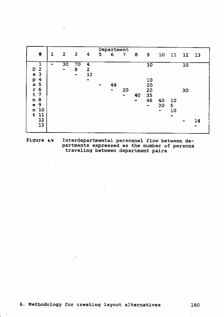
Department1 2 3 4 5 6 7 8 9 10 11 12 131 - 30 70 4 10 10

D 2 — 8 2e 3 - 13p 4 - 10a 5 — 44 20r 6 - 20 20 30t 7 - 40 35m 8 - 46 40 10e 9 - 30 5n 10 - 10t 11 -12 - 14

13 -

Figure 6% Interdepartmental personnel flow between de-partments expressed as the number of personstraveling between department pairs


Department1 2 3 4 5 6 7 8 9 10 11 12 13

1 - 5 2D 2 - 8e 3 — 10p4 -a 5 —r 6 -t 7 -m 8 —e 9 — 5 5n 10 -t 11 -12 -13 —

Figure as Closeness rating for Common personnel (Max10,Min O)

}


Department1 2 3 4 5 6 7 8 9 10 11 12 13

1 -D 2 -e 3 — 10p4 -a 5 - 10r 6 - 8 8t 7 - 9m 8 - 7 3e 9 — 10n 10 -t 11 -12 -13 -

Figure 61 Closeness rating for Common data used (Max10,Min0)l


Department# 1 2 3 4 5 6 7 8 9 10 11 12 13

1 - 1D 2 - 1e 3 - 1p 4 —a 5 ·r 6 -t 7 -m 8 -e 9 -n 10 -t 11 -12 — 1

13-

Figure 6.7 Closeness rating for Contact necessary (Max· 10,Min O)


W

Department# 1 2 3 4 5 6 7 8 9 10 11 12 13

1 -D 2 -e 3 —p4 —a 5 - 2 1 1r 6 — 2 2 2t 7 - 2 2m 8 - 2 2e 9 - 2n 10 -t 11 -12 —

13 -

Figure 68 Closeness rating for Convenience (Max 10,Min0)

}


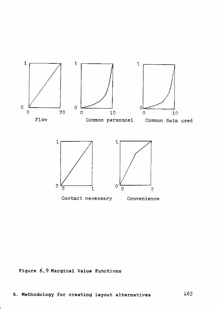
0 70 0 10 0 10Flow Common personnel Common data used

I

O 0 1 O 0 .2Contact necessary Convenience

Figure .6.9 Marginal Value Functions


Department1 2 3 4 5 6 7 8 9 10 11 12 13

1 .00 .44 .31 .02 .00 .00 .00 .00 -04).00 .00 .04*.00D 2 .44 .00 .36 .01 .00 .00 .00 .00 .00 .00 .00 .00 .00e 3 .31 .36 .00 .66 .00 .00 .00 .00 .00 .00 .00 .00 .00p 4 .02 .01 .66 .00 .00 .00 .00 .00 .04 .00 .00 .00 .00a 5 .00 .00 .00 .00 .00 .44 .08 .08 .09 .00 .00 .00 .00r 6 .00 .00 .00 .00 .44 .00 Q20?.10 .20 .00 .00 .13 .00t 7 .00 .00 .00 .00 .08 102 .00 .29 .25 .00 .00 .00 .00m 8 .00 .00 .00 .00 .08 .10 .29 .00 .31 .17 .15 .00 .00e 9 .04 .00 .00 .04 .09 .20 .25 .31 .00 .39 .04 .00 .00n 10 .00 .00 .00 .00 .00 .00 .00 .17 .39 .00 .04 .00 .00t 11 .00 .00 .00 .00 .00 .00 .00 .15 .04 .04 .00 .00 .00

12 -04 .00 .00 .00 .00 .13 .00 .00 .00 .00 .00 .00 .3613 .00 .00 .00 .00 .00 .00 .00 .00 .00 .00 .00 .36 .00

Figure 6Jo Preference matrix


1

TPRA is the sum of preference ratings of department pairs

divided by the distances between them. TPRA is used here to

compare the layouts generated by CORELAP, ALDEP, and the

proposed procedure because the previously described measure

of TPR (see section 3.3.2.1) is not applicable to the layouts

generated by CORELAP and ALDEP.

The layout created by CORELAP is shown in Figure 6.11. The-

TPRA value of the layout is 247. Figure 6.12 shows the layout

created by ALDEP and the TPRA value of this layout is 142.

Note that the layout generated by ALDEP gives a smooth

boundary and departments can assume other shapes besides be-

ing rectangular, whereas CORELAP generates a zig-zag boundary

for the departments and the department shapes are always

rectangular.

6.6.3 RESULTS OF EXPERIMENTATION WITH THE PROPOSED PRCCEDURE

Next, we present results obtained using the proposed proce-

dure. The results are presented both for the case of equal

and unequal department sizes. Figure 6.13 shows the initial

layout and the final layout (A1) created by the proposed

procedure when the departments are assumed to be unequal

‘during the generation of the initial layout. Figures 6.14,

_ 6.15, 6.16, 6.17, 6.18, and 6.19 depict·initial and final

layouts created. under several conditions by the proposed


Ü

22 .

ll‘“

6¤1213 ·

Fiqureéll Layout created by CORELAP


Figure6.12 Layout created by ALDEP

6. Methodology for creating layout alternatives T.69

procedure when the departments are assumed to be of equal

sizes during the generation of the initial layout. Figure

6.14 depicts the layout (Bl) obtained when only the first

closeness criterion (flow) is in consideration. Similarly,

Figures 6.15, 6.16, 6.17, and 6.18 depict layouts designated

B2, B3, B4, and B5 when the criterion of common personnel,

common data, necessary contact, and convenience, respec-

tively, are in consideration individually. Figure 6.19 re-

presents the layout (B6) obtained when all criteria are in

consideration together.

All scores related to the layouts depicted in Figures 6.11

to 6.19 are summarized in Figure 6.20. The TMAX score shown

in Figure 6.20 is computed by making the scaling constant of

the considered criterion to be 1.0 and the others to be zero.l

It also shows values of TPR for the layouts generated by the

proposed procedure under various conditions. It is clearly

indicated by Figure 6.20 that better results are obtained

when all criteria are considered together.

A detailed experimentation is next carried out as depicted

in Figure 6.21. Seventy preference matrices of problems of

sizes 9 to 23 departments are randomly generated by the ma-

trix generator shown in Appendix C. Both CORELAP and the

proposed procedure are used to create layouts for these ma-

trices. Figure 6.21 presents scores of layouts created by

}


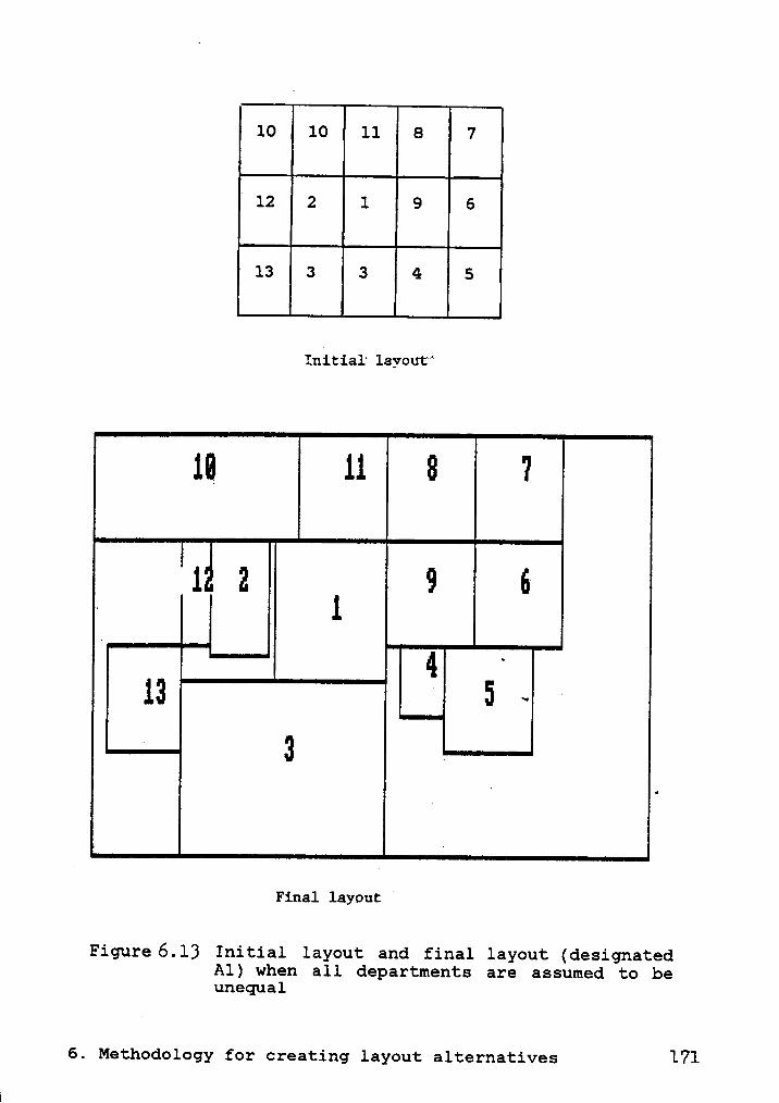
10 10 ll¤

712 2 1 ll2llll

Initial layout"

Final layout;‘

Figure 6.13 Initial layout and final layout (designatedAl) when all departments are assumed to beunequal


77 l 7 7 H77 Il 7 I77 lllInitial layout

B¤7777777ql ‘

019 77

Final layoutl ·

Figure 6,1/-L Initial layout and final layout (designatedBl) for the criterion of Interdepartment flow

6. Methodology for creating layout alternatives-‘-72

10 12 13 7¤I 21 1 II

IIIIInitial layout

l

13 ?1

'|llH

_

_

Final layout _

Figure 6.15 Initial layout and final layout (designatedB2) for the criterion of Common personnel

6. Methodology for creating layout alternatives 1-73

ll 11 I1 lll11 11 lllInitial layout

1

11Final layout1

Figure6.l6 Initial layout and final layout (designatedB3) for the criterion of Common information

6. Methodology for creating layout alternatives 17a

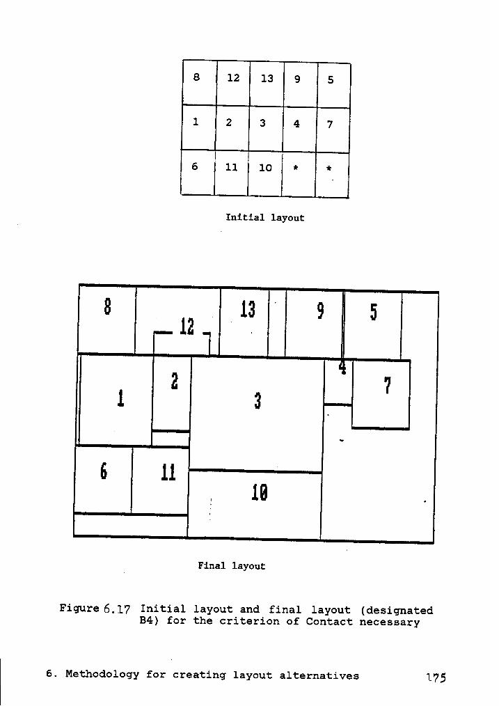
E 12 11 ll1 1 ll 14 1

6 11 10 *

Initial layout

Final layout

Figure 6.17 Initial layout and final layout (designatedB4) for the criterion of Contact necessary

, 6. Methodology for creating layout alternatives 175

1 1 ll 111 llll11 11 11 ll

Initial layout

J13 H

IFinal layout

Figure 6.l8 Initial layout and final layout (designatedB5) for the criterion of Convenience

6. Methodology for creating layout alternatives 17*5

12

I

13 11 1 2

6 6 ll 66 66 Il

l Initial layout

1 13 111¤7 u E

IllFinal layout·

Figure 6,19 Initial layout and final layout (B6) when allcriteria are considered together


ScoreLayout GenerationProcedure TMAX TPRA TPR

CORELAP — 247 —

ALDEP — 142 —

Proposed procedure assuming unequal — 273 10.04size departments and all criteriaconsidered together(Layout Al)

Proposed procedure assuming equalsize departments for

Flow criterion only 12.78 240 8.60(Layout Bl)

Commmon personnel 2.89 207 7.70criterion only ·(Layout B2)

Commmon information 6.97 236 8.10criterion only(Layout B3)

Contact necessary 8.00 149 6.10criterion only(Layout B4)

Convenience 17.67 225 7.90criterion only(Layout B5)

‘All criterion together · 264 9.10(Layout B6)

Figure $$0 Scores of Layouts Created by CORELAP,ALDEP,and the Proposed Procedure Under VariousConditions.

6. Methodology for creating-layout alternatives 178

CORELAP and the proposed procedure and the percentage im-

provement of the proposed procedure over CORELAP. A graph

which depicts the percent improvement (Z) of the proposed

procedure over CORELAP as a function of the problem size (n)

is shown in Figure 6.22. The graph shows a decreasing trend

in percentage improvement when the problem size is small (n=9

to 14). This trend ceases at the medium size problem (n=l4

to 15) and becomes an increasing trend for larger problem

size (n=16 to 23). The nature of this relationship between

the performance of CORELAP and the proposed procedure may be

explained with reference to Figure 6.23 which speculates

relative performances of both of these procedures, compared

to the optimal solution, as a function of problem size. The

exact performance of these procedures are difficult to meas-

ure due to the unavailability of the optimal solution for

layouts when n>5. For n=<2, both procedures generate optimal

layouts. The proposed procedure continues to generate opti-

mal layouts for n=<5 because the problem is solved exactly.

As the problem size increases, the performance of both the

procedures first decrease and then tend to stabilize. Since

CORELAP is basically a construction routine, its performance

is lower than that of the proposed procedure. The perform—V

ance of CORELAP decreases more uniformly than that of the

proposed procedure. Because of this nature of the graphs,

the difference between the performances of CORELAP and the


proposed procedure first decreases and then increases with

an increase in problem size. x'

Next, we discuss how the total preference ratings (TPR) (de-

scribed in section 3.3.3) can be used in the overall decision

process to choose the lbest layout alternative. The TPR

preference function must first be evaluated as described in

· section 3.3.3. In order to evaluate a preference function,

an upper bound value must be determined for which a prefer-

ence rating of 1 is asssumed. We show here one way of com-

puting an upper bound of TPR. Let Tmax be the TPR value when

the scaling constant of criterion k is set to 1.0 and the

scaling constants of other criteria are set to O. The upper

bound is then computed as followsz

nUB

=k;1Tmaxksck

where

sck = actual scaling constant of attribute k.

Thus, for the example problem bf Figure 6.20,

UB = 12.78(.3)+2.89(.15)+6.97(.15)+8.00(.3)+17.67(.1)

= 9.48 .

A similar method can be applied to find the upper bound of

TPRA if TPRA is used as the overall decision criterion.


Prob1•n TPRR aF TPRH 6$ P•rc•nt•ga HuerageSize Propoxed CORELBP Inprouenent Pnrcentagein) Pracedure C2) Inprouenent

9 212.66 198.00 7.409 240.16 226.00 6.279 227.16 205.00 10.819 193.83 183.33 5.739 239.66 225.00 6.529 239.16 224.16 6.699 260.66 241.00 8.16 7.37¤ 49. -62. - .¤

289.20 272.86 5.99236.40 222.23 6.38250.10 238.00 5.08198.00 183.57 7.86 6.48

E 'I(_

I 2Z11.... ..1.. ...212 214.00 1·1.—¤ .-12 187.73 175.40 7.0312 360.02 340.29 5.8012 355.51 338.26 5.1012 327.07 310.91 5.2012 351.46 332.73 5.6312 388.61 368.66 5.4112 375.23 359.60 4.3512 344.43 335.83 2.562 ·- 375.40 7.0813 189.00180.737

251.97 239.17 4.9614 494.33 ·8 . ~ .14 422.40 411.96 2.5314 437.53 424.73 3.0114 470.56 459.26 2.4614 474.60 461.46 2.8514 484.70 462.20 4.8714 463.73 442.19 4.8714 503.63 485.50 3.73

· -57 40 439.36 4.11 3.33

381.60 370.00 4.11Ä°’°‘*° ***2*** ÄGZEI

1 · .4 r. ¤ ‘·1. ....1.....1.17

428.90 41 .u¤ -. -17 632.71 602.01 5.1017 648.37 620.45 4.5017 623.42 599.85 3.9317 678.85 652.38 4.0617 621.13 607.63 2.2217 641.85 607.65 5.6317 711.41 678.68 4.82 4.33

1. . Z" J. .‘

X11 -1..... -1..... ..11.483.06 460.28 4.752* 22 ' ~I,I ,

._

895.35 844.40 6.03858.55 831.59 3.24905.54 864.57 4.74849.26 807.48 5.17895.44 841.16 6.45 5.32

2.1 J. '- H ••6-2

21 906.08 848.83 6.7421 949.94 898.07 5.7821 917.13 858.53 6.8321 898.39 843.72 6.4821 957.04 893.03 7.17 6.77{ J-.;°·22

975.86 914.60 6.69 6.792 23 1¤· .1 ¤ •.·= .-23 1066.51 992.11 7.5023 1180.61 1100.29 7.3023 1071.44 1003.23 6.8023 1014.80 947.58 7.09 6.87

Figure 6.21 Scores of Layouts generated by CORELAP and- the Proposed Procedure for problem of dif-

ferent size.


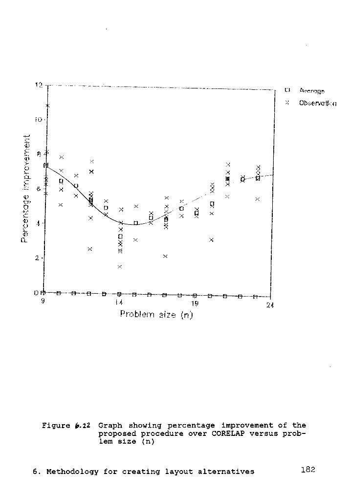
1 .. „.. .. _..- ..-.. .....-. .... ..;,4.... 2.- ..,.....-........„„.........„.„

cwürügn

I I Z¢·¥ ;iJI:»=;•~em:1II‘·;;:+·‘4I

II¤;...• · |I

I I

5;. éITE

>< L.; M2; FI „.... E II"""IÄ.; {L j:·{ .. .

III

*13.· . .

2::, ,•·•__._

M 'M-. ' ' ·?/ Ix:

'ILI 4'/ I

.· ¤

LTLI IIII

IÜ IiII“”°EI”'°’°'"I°I”°""‘I?II‘““"‘B” ""fB·"**FI··——EI—--··-—Er—~+_+·~——;3;-—----5-.-B..F.}__.--....-.H„„_,_I

III I ·I 1 5;.4.FI 4;:; bl In ff;

Figure ß. 22 Graph showing percentage improvement of theproposed procedure over CORELAP versus prob-lem size (n)


.. .„....,...„.......„ ..............-,... ,.,.-................-.....-—.T..........,—..I....„.......................,.....„-.... .,........................,,.„.....,...„..............,.,...... .

I-\

j N = °I TO :5 ‘

\ I \I \\ I II ‘

I I\_l ,

\*-11\I\_ f „\

I

I\gg]

‘\. -

IXx

II

I.-,.....-....,.,...........I,...I,....•,,... „....„....,..,_T..,, .._...__,,„„,_I..,„__,________„.-.,.,,I.,.„,.......-....-_,.........,..I-....„..„.,--„.-..„....I,.....iII;> I4 IE am :14

Figure 6.25 Performance curves of CORELAP and the pro-- posed procedure versus problem size

6. Methodology for creating layout alternatives I-83 I


In this chapter a method of determining relative department

locations was developed. This method is based on the formu-

lation of the layout problem as a quadratic assignment prob-

lem. The proposed procedure for the solution of the QAP is

specially designed in order to be implemented on an IBM PC.

Three construction and two improvement routines are jpro—

grammed on the IBM PC as a part of the layout design package

that is developed. The quality of the layout obtained can

be improved by running through the improvement routine se-

veral times. The results from this methodology are used to

create a final layout where actual department sizes and other

criteria are considered. A procedure to create the final

layout was also described. Finally, the results of using the

initial and the final creation process on the example problem

were presented. The proposed procedure gives layouts which

are consistently better than those obtained using CORELAP.

In addition, the proposed method allows the designer to

interact during the design process to make appropriate ad-

justments on the final layout. _


7. SUMARY, CONCLUSION, AND RECOMMENDATIONS

This study has presented a decision theoretic approach and a

computerized decision support system for solving the general

layout design problem. The research was divided into seven

tasks as follows.

1. Review of the literature on layout design approaches.

2. Review of the literature on decision theory.

3. Development of a decision theoretic approach to the lay-

out design problem.

4. Review of the literature on quadratic assignment problem.

5. Development of heuristics for solving the quadratic as-

signment problem.

6. Development of new theoretical results to justify the

decision theoretic approach taken.

7. Development of a computerized decision support system.

7. Summary, Conclusion, and Recommendations 185

This chapter summarizes the study and gives suggestions for

further research.


A major motivation of the research came from the fact that

most of the layout design approaches reported in the litera-

ture are concerned only with economic justification, bas-

ically, that of material handling cost. Some of the studies

consider qualitative factors and use closeness ratings to

measure these factors. Generally, a scale of A, E, I, O, and

U is used to represent closeness ratings between pairs of

departments. This research developed a layout design ap-

proach which accounts for multiple criteria in a systematic

«fashion. The results presented in Chapter 6 have shown that

this multicriteria approach gives better solutions than a

single—criterion approach.

7.1.1 A DECISION THEORETIC APPROACH TO LAYOUT DESIGN

Layout design has rarely been addressed as a multicriteria

problem. Chapter 3 of this study presented an approach for

layout design, taking multicriteria into account. This ap-

proach is a systematic way of measuring the closeness rating

for any· departmental pair. A function representing the

closeness rating between any departmental pair is con-

7. Summary, Conclusion, and Recommendations 186 ·'

structed. Since the layout criteria may be measured on dif-

ferent scales, they are converted into a preference scale.

The criteria are then combined by either additive, multipli-

cative, or multilinear functions. The combined criterion,

for any departmental pair, is then rated. This results in

closeness ratings of department pairs. The departments are

then assigned to locations so that the sum of closeness

ratings is maximized. A set of overall evaluation criteria

is used to evaluate the final layout.

7.1.2 JUSTIFICATION OF THE DECISION THEORETIC APPROACH

The approach developed in this study involves criteria which

are measured on various scales. The first task in this case

is to convert these scales into a unique scale such that all

criteria can be combined. The combining of functions may

take several forms, for example, additive, multilinear, and

multiplicative. In order to take any of these forms, the

attributes (criteria) set must satisfy some conditions. In

the literature, axiomatic systems defined for attributes,

which are measured on continuous scales, have been developed.

However, these axiomatic systems are not applicable for the

case where attributes are discrete or binary (Deutsch and

Malmborg, 1984). The insufficiency of the present axiomatic

system for the discrete and binary cases was presented in

Chapter 3. In Chapter 5, the axiomatic system for mixed at-

7. Summary, Conclusion, and RecommendationsI

187

tributes which includes continuous, binary, and discrete at-

tributes was presented. The necessary theoretical results

for the additive, multilinear, and multiplicative forms,

based on this axiomatic system, were presented.

7.1.3 SOLUTION PROCEDURES FOR THE QUADRATIC ASSIGNMENT

PROBLEM U

In Chapter 6, a method of determining relative department

locations based on closeness ratings was presented. The ob-

jective of the method was to optimize closeness ratings.

This involved formulation of the problem as a quadratic as-

signment problem which attempts to allocate departments to

locations. Three construction and two improvement heuristics

were developed and presented.

The successful heuristics reported in the literature are

computationally intensive and require a tremendous amount of

computer memory. The solution procedures for the quadratic

assignment problem are specially designed by this research °

so that they can be implemented on an IBM PC with 256K RAM.

Since the computer has limited calculation speed and computer

memory, the improvement heuristic developed is designed as a

polynomial time heuristic which is effective with respect to

the quality of solutions obtained, while at the same time not

being computationally intensive.


7.1.4 DECISION SUPPORT SYSTEM FOR THE LAYOUT DESIGN PROBLEM

The decision support system developed in this research, to

aid the layout design is an interactive computer software

which utilizes both the human and machine capabilities. In

a layout design problem, the “human. is necessary for the

evaluation of an ill-structured criterion, creative design,

and practical design. The machine is needed for handling

large amounts of information pertaining to material handling

costs and closeness ratings for the various departments in-

volved in a problem. The computer software package was de-

veloped based on the decision support systmn presented in

Chapter 4. This package is divided into three phases asl

follows.

1. Data Acggisition: This phase prepares primary information

for the layout problem. This includes five programs; namely,

the scaling constant assessment program, the marginal value

function assessment program, the facility specification pro-

gram, the adjacency requirement program, and computing the

preference matrix program. Two of these programs, namely,

the scaling constant assessment program and the marginal

value function assessment program, utilize the IBM PC graphic

capability to aid the assessment procedure.


2. Layout construction: This phase includes two programs,

namely, the initial layout creation program and the final

layout creation program. They utilize information prepared

in phase 1, and generate layout alternatives using the pro-

posed algorithm. The initial layout creation program deter-

mines relative department locations by using three

q construction and two improvement heuristics. The improvement

heuristics are based on the solution to a quadratic assign-

ment problem and pairwise interchanges among departments.

Any combination of these heuristics can be utilized to solveéthe

problem. Results from the initial layout creation pro-

gram merely give relative department locations since it as-

· sumes equal department sizes. Consequently, the purpose of

the final layout creation program is to create layout alter-

natives with exact department sizes using the results from

t the initial layout creation program.

3. Overall evaluation: This phase consists of four programs

to prepare data and to compute final layout alternative

scores. There are two assessment programs, namely, the

scaling constant assessment program and the marginal value

function assessment. progrann These two programs prepare

value functions for the overall decision criterion. The

other two programs compute the final scores.


7.1.5 RESULTS OF EXPERIMENTATIONI

An extensive experimentation was conducted to test the per-

formance of the proposed procedure for the layout design

problem. The results indicate that this procedure is easy

to use and it generates better solutions than those generated

by CORELAP.

7.2 RECOMENDATION

This section lists some topics for future study and improve-

ment as follows.

1. Decision theory: An axiomatic basis for value functions

defined on a mixed attributes set was presented in chapter

5. The compensatory conditions defined must hold to allow

the additive value function form to be used. Should the

condition be verified, the number of all possible Verifica-

tions become very large when the function involves multilevel

attributes. Gorman (1968) has done some work to reduce the

number of independent verifications for the axiomatic system

defined on continuous attributes. A similar work concerning

our axiomatic system should be investigated in order to sim-

plify the Verification procedure. Otherwise, alternative

approaches or axiomatic systems for the mixed attribute set

will be a promising research area.


2. Computer package: The computer package has been developed

as a tool to aid layout design. The additive form is used

for the combination of criteria. The total preference func-

tion is formulated as a quadratic assignment problem. An

improvement can be made in the program by developing a better

data preparation scheme to accommondate unequal size depart-

ments. Currently, some of the data preparation for unequal

size departments is done manually. In addition, the computer

package should provide other value function forms, for exam-

ple, multilinear and multiplicative. Another potential im-

provement concern providing more user-friendly commands in

the program.

3. Other applications of decision theory: Typically, prob-

lems in manufacturing system design involve several economic

and performance related criteria. In this research, we have

developed results for multicriteria functions involving dis-

crete and continuous attributes. These were demonstrated in

this research specifically on the layout design problem.

However, the same functions, and modifications thereof, can

be investigated for application to other multicriteria prob-

lems.


BIBLIOGRAPHY ·

Apple, J. M., 1977. Plant Layout and Material Handling 3rdEdition, John Wiley & Sons, New York.

Apple, J. M. and Deisenroth, M. P., 1980. "A ComputerizedPlant Layout Analysis and Evaluation Technique (PLANET)",Proceeding AIIE 1980, pp.121-127.

Armour, G. C. and Buffa, E. S., 1963. "A Heuristic Algorithmand Simulation Approach to Relative Location of Facili-ties", Management Science, 9(1), pp.294-309. .

Bazaraa, M. S., 1975. "Computerized Layout Design: A Branchl

and Bound Approach", AIIE Transactions, 7(4), pp.432-438.

Bazaraa, M. S. and Goode, J. J., 1977. "The TravellingSalesman Problem: A Duality Approach", Mathematical Pro-gramming, v13, pp.221-237.

Bazaraa, M. S. and Sherali, H. D., 1980. "Benders Partition-ing Scheme Applied to a New Formulation of the QuadraticAssignment Problem", Naval Research Logistics Quarterly,v27, pp.29—41.

Bazaraa, M. S. and Sherali, H. D., 1982. "On the Use of Exactand Heuristics Cutting Methods for the Quadratic Assign-ment Problem", Journal of Operations Research Society,v33, pp.991-1003.

Block, T. E., 1978. "A New Construction Algorithm for Facil-ities Layout", Journal of Engineering Production, n2,pplll-

Buffa, E. S., Armour, G. C., and Vollmann, T. E., 1964. "Al-locating Facilities with CRAFT", Harvard Business

A Review, 42(2), pp.136-159.

Burkard, R. E. and Stratmann, K. H., 1978. "Numerical ln-vestigation on the Quadratic Assignment Problem", NavalResearch Logistics Quarterly, v25, nl, pp.129-248.

Cabot, V. A. and Francis, R. L., 1970. "Solving Certain Non-convex Quadratic Minimization Problems by Ranking the Ex-treme Points", Operations Research, v18, pp.82-86.

Dawes, R. M. and Corrigan, B., 1974. "Linear Models in Deci-sion Making", Psychological Bulletin, pp.97—106.

Bibliography 193

Debreu, G., 1960. "Topological Methods in Cardinal UtilityTheory", Mathematical Method in the Social Science,pp.16-26.

Deutsch, S J. and Malmborg, C. J., 1984. "An Axiomatic Basisfor Multiattribute Value Functions Defined on Binary At-tributes", Working Paper, School of Industrial Engineeringand System Engineering, Georgia Tech and Department ofIndustrial Engineering and Operations Research, VirginiaTech.

Deutsch, S. J. and Malmborg, C. J., 1985. European Journalof Operational Research, v19, n2.

Deutsch, S. J. and Malmborg, C. J., 1985. "Interdependentadditive conjoint structures", European Journal of Opera-tional Research, vl3, n4.

Drezner, Zvi, 1980. "DISCON: A New Method for the LayoutProblem", Operations Research, 28(6), pp.1375-1384.

Dutta, K. N. and Sahu, S., 1982. "A Multigoal Heuristic forFacilities Design Problem: MUGHAL', Int. J. Prod. Res.,20(2), pp.147-154.

Dyer, J. S. and Sarin, R. K., 1979. "Measurable Multiattri-bute Value Functions", Operations Research, 27(4),pp.810-822.

Einhorn, IL J. and Hogart, R. M., 1975. "Unit WeightingSchemes of Decision Making", Organizational Behavior andHuman Performance, 13, pp.171-192.

Filley, R. D., 1985. "Three Emerging Computer TechnologiesBoost Value of, Respect for Facilities Function", Indus-trial Engineering, 17(5), pp.27-39.

Fishburn, P. C., 1970. Utility Theory for Decision Making,John Wiley & Sons Inc., New York.

Foulds, L. R. and Robinson, D. F., 1978. "Graph theoreticHeuristic for the Plant Layout Problem", Int. J. Prod.Res., 16(1), pp.27-37.

Francis, R. L. and White, J. A., 1974. Facility Layout andLocation: An Analytical Approach, Prentice-Hall Inc.,Englewood Cliffs, New Jersey.

Gardiner, P. C., 1977. "Decision Spaces", IEEE Transactionson Systems, Man, and Cybernetics, SMC-7(5), pp.340-349.

Bibliography 194

Gaschutz, G. K. and Ahrens, J. H., 1968. "Suboptimal Algo-rithm for the Quadratic Assignment Problem", Naval Re-search Logistics Quarterly, v15, pp.49-62.

Gavett, J. W. and Plyter, N. V., 1966. "The Optimal Assign-ment of Facilities to Locations by Branch and Bound", Op-erations Research, v14, pp.210—232.

Gilmore, P. C., 1962. "Optimal and Suboptimal Algorithms forthe Quadratic Assignment Problem", SIAM Journal on AppliedMathematics, v10, pp.305-313.

Gorman, W. M., 1968a. "The Structure of Utility Functions",Review of Economic Studies, 35, pp.367—390.

Gorman, W. M., 1968b. "Conditions for AdditivitySeparabilities", Econometric, 36, pp.605-609.

Graves, G. W. and Whinston, A. B., 1970. "An Algorithm forthe Quadratic Assignment Problem", Management Science,v17, pp.453—47l.

Hall, K. M., 1970. "An r—Dimensional Quadratic PlacementAlgorithm", Management Science, v17, pp.219-229.

Hillier, F. S., 1963. "Quantitative Tools for Plant LayoutAnalysis", The Journal of Industrial Engineering, v14,pp.33—40.

Hillier, F. S. and Connors, M. M., 1966. "Quadratic Assign-ment Problem Algorithms and The Locations of IndivisibleFacilities", Management Science, vl3, pp.42-57.

Johnson, R. V., 1982. "sPAcEcRAET for Multi—floor LayoutPlanning", Management Science, 28(4), April, pp.406-417.

Kaufman, L. and Broeckx, F., 1978. "An Algorithm for theQuadratic Assignment Problem Using Benders' Decompos-ition", European Journal of Operational Research, v2,pp.207—211.

Keeney; R. L. and Raiffa, H., 1976. Decisions with MultipleObjectives: Preferences and Value Tradeoffs, John Wiley &Sons, New York.

Koopmanns, P. C. and Beckmann, M. 1957. "Assignment Problemsand the Location of Economic Activities", Econometrica,v25, PP•53-76.

Bibliography 195

Krantz, C. H., Luce, R. D., Suppes, P., and Tversky, A.,1971. Foundations of Measurement, Volume I: Additive and

°Polynomial Representations, Academic Press, New York.

Krejeirik, M., 1969. "RUGR Algorithm', Computer AidedDesign, Autumn.

Land, A. N., 1963. "A Problem of Assignment with InterrelatedCosts", Operational Research Quarterly, v14, pp.185-198.

Lawler, E. L., 1963. "The Quadratic Assignment Problem",Management Science, v19, pp.586-599.

Lee, R. C. and Moore, J. M., 1967. "CORELAP-Computerized Re-lationship Layout Planning", Journal of Industrial Engi-neering, 18(3), pp.l95-200.

Lewis, W. P. and Block, T. E., 1980. "On the Application ofComputer Aids to Plant Layout", Int. J. Prod. Res., 18(1),pp.11-20.

Los, M., 1977. "Simultaneous Optimization of Land Use andTransportation: A Synthesis of the Quadratic AssignmentProblem and of the Optimal Network IProblem", RegionalScience and Urban Economics.

Love, R. L. and Wong, J. Y., 1976. "Solving Quadratic As-signment Problems with Rectangular Distances and IntegerProgramming", Naval Research Logistics Quarterly, 23(3),pp.623—628.

Malmborg, C. J., 1981. Ph.D Dissertation, Georgia Tech.

Malmborg, C. J. and Sarin, S. C., 1984. Plant Layout and De-sign Course Work Book, Department of Industrial Engineer-ing and Operation Research, Virginia Tech.

Mirchandani, P. B. and Obata, P., 1979. "Locational Deci-‘sions with Interactions between Facilities: The QuadraticAssignment Problmn - A Review", Working Paper PS-79-1,Rensselaer Polytechnic Institute.

Moore, J. M., 1974. "Computer Aided Facilities Design: AnInternational Survey", Int. J. Prod. Res., 12(2). __

Muther, R. M., 1955. Practical Plant Layout, McGraw-HillInc., New York.

Muther, R. M., 1961. Systematic Layout Planning, IndustrialEducation Institute, Boston, Mass.

Bibliography 196

Muther, R. and McPherson, K., 1970. "Four Approaches to Com-puterized Layout Planning", Industrial Engineering, 2(2),pp.39-42.

Nugent, C. E., Vollmann, T. E., and Ruml, J., 1968. "An Ex-perimental Comparison of Techniques for the Assignment ofFacilities to Locations", Operations Research, v16,pp.l50-173.

O'Brien, C. and Barr, E. Z. A., 1980. "An Interactive Ap-proach to Computer Aided Facility Layout", Int. J. Prod.Res., 18(2), pp.20l—211.

Patel, A. M. et. al., 1976. “Prepartioning as a Means ofEnhancing Pairwise Interchange Solution to Quadratic As-signment Problems", Computer and Operations Research, V3,pp.49-56.

Pegels, C. C., 1966. "Plant Layout and Discrete Optimiza-tion", International Journal of Production Research, V5,pp.81-92.

Pierce, J. F. and Crowston, W. B., 1971. "Tree Search Algo-rithms for the Quadratic Assignment Problems", Naval Re-search Logistics Quarterly, v18, pp.1-36.

Rajgopal, P., 1985. "A Flexible Construction and ImprovementHeuristic for the Quadratic Assignment Problem", MasterThesis, Virginia Tech.

Reed, R. Jr., 1961. Plant Layout, Irwin Inc.

Rosenblatt, M. J., 1979. "A facilities Layout Problem: AMulti-goal Approach", Int. J. Prod. Res., 17(4),pp.323-332.

Roucairol, C., 1978. "A Reduction Method for the Quadratic

Assignment Problems", 3rd symposium Uber Operations Re-search, University Mannheim, October.

Seehof, J. M. and Evans, W. O., 1967. "Automated Layout De-sign Program", Journal of Industrial Engineering, 18(12),pp.690-695. .

Seppanen, J. and Moore, J. M., 1970. "Facilities Planningwith Graph Theory", Management Science, l7(4), December,pp.242-253.

Seppanen, J. and Moore, J. M., 1975. "String Processing Al-gorithms for Plant Layout Problems", Int. J. Prod. Res.,l3(3), pp.239-254.

Bibliography 197

Smith, H. C. T., 1975. "A Computational Comparison of an Im-proved Pair Assignment Algorithm and a Pair Exclusion Al-gorithm for the Quadratic Assignment Problem", AD—AO19799.

Vollmann, T. E., Nugent, C. E., and Zartler, R. L., 1968."A Computerized Model for Office Layout", The Journal ofIndustrial Engineering, v19, pp.321—329.

Bibliography 198

APPENDIX A. DESCRIPTION OF PROGRAMS IN THE DECISION SUPPORT

SYSTEM

MAIN: MAIN program accesses to three programs-MAINl, MAINZ,

and MAIN3.

MAIN1: This is za Data Acquisition control access program

which allows the user to link to MAIN11, MAINIZ, MAINl3,

MAINI4, and MAINl5.'

MAINZ: This is a Layout Construction control access program

which links to MAIN21 and MAINZZ.

MAIN3: This is a Ewaluation control access program which

links to MAIN3l, MAIN3Z, MAIN33, and MAIN34.

MAIN11: This program helps in interactively assessing scaling

constants of closeness related criteria.

MAIN12: This program helps in interactively assessing mar-

ginal value functions of the closeness related criteria.

MAIN13: This program acquires department specifications which

include department names and sizes.

Appendix A. Description of Programs in the DecisionSupport System ‘ « 199

MAINI4: This program acquires criteria rating for all de-

partment pairs.

MAINl5: This program uses data acquired in MAINl1, MAINl2,

MAINl3, MAINI4, and MAINl5 to compute the preference matrix.

This matrix is used in the Layout Construction phase.

MAIN2l: This program creates initial layouts which give rel-

ative department locations. The designer must specify block

plan layout. Any combination of construction routines (CRl0,

CRZO, or CR30) and improvement routines (IMPl and CQAP) can

be selected. Then, the computer produces initial layouts and

compute their scores.

MAIN22: This program allows the designer to create final

layouts using the actual department sizes.

MAIN3l: This program assesses scaling constants of the over-

all decision criteria.

MAIN32: This program assesses marginal value functions of the

overall decision criteria..

MAIN33: This program acquires criteria rating for all layout

alternatives.

Appendix A. Description of Programs in the DecisionSupport System 200

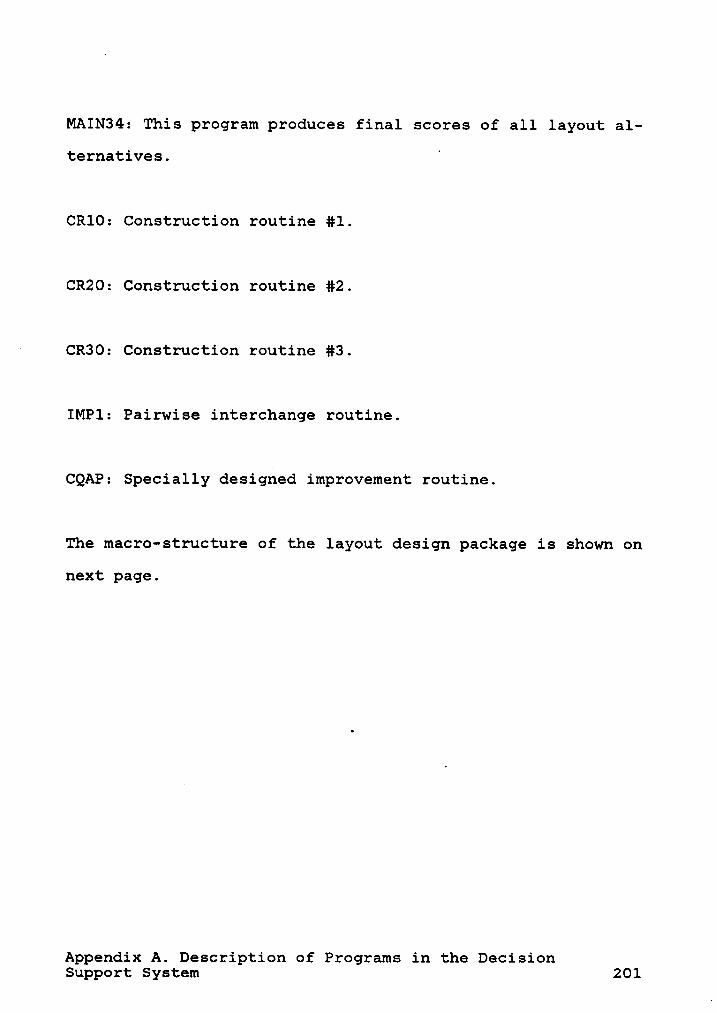
MAIN34: This program produces final scores of all layout al-

ternatives. °

CR10: Construction routine #1.

CR20: Construction routine #2.

· CR30: Construction routine #3.

IMP1: Pairwise interchange routine.

CQAP: Specially designed improvement routine.

The macro—structure of the layout design package is shown on

next page.


EPI·-I2l·-·*i—·'

EPH2HN

3 EP P ·I-·I I—IZ ZH HUO

EPI—I

W 2O l·-*'1 POIcn E"* E

ZO

I—·•

cl- O U1

ä E ~=<v 0 E §

!> •—•O I-I 2H: O 2 E

W- N Pc+ N

b—• Q-;Z3' O ZCD N

EE" O PB7 W H°< W 2O O. N5 N¢.+

HU E ECD "U P:11 H HI-•· 2§ U)

O H

"U9:"U E

o :>:¤:' HN 2Ut; U0CD N

EP

E+—• _

P 2H U>2U0U)

EPH2

. UJ· I?


APPENDIX B. A COMPUTER RUN OF THE EXAMPLE PROBLEM

Diagrams 1, 2, 3, and 4 are shown on the following pages,

depict keys to accessing each screen. Legend N1.N2 : N1 re-

presents program number and N2 represents the screen number

created by each program. For example, see diagram 2, press

pf8 to go from 12.6 to 1.1, press 2 and <return> to go from

1.1 to 12.1.

Appendix B. A Computer Run of the Example Problem 203

uacuQ .

U•-··. ¤¤ ·

W $9g ES M5

U¤

ä N =·•-·u·

. sb . .0*3 .Ps° \S U ·=¤zv•-• * 6

a>coUä' 4

· E_ «x=

-204

II- I-¤ \. 1-• :¤ 6-·I-•

‘—

:Q•\Q : I

•I \\~

x MJ • r-•'

‘,'*5\_/ N ·· *\;°,‘:

RT$\

N N EÄ? g *. •Ln

‘

" I_ ¤¤ . .I-* I·-*°\

'P j *·* I Il /

.I-••O

N ®an I-‘ II-! I-*

ä - F :¤ F zu F \ _•-•M: N ·

‘

F ¤ I-· l.

gg E 'E >O [IV

· I-‘— ·-zu·=¤ -- J: ·oo >D

¤O •-4~O dj ·‘

cz um. . >

I-•\_ ’ I-• xUR · U1 \

l

.‘ ·· . 205

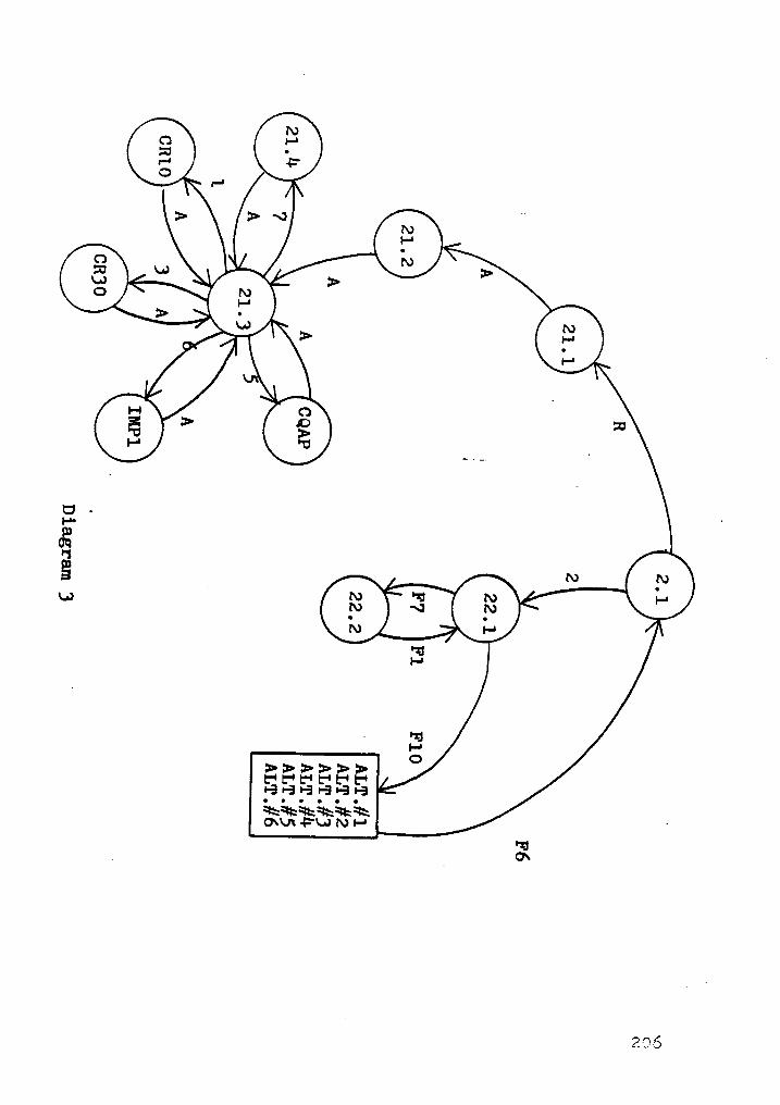
„. 8w

·‘

aß’ “’

8Q.Hg .

m

A)

üßw~

— wI-*

Qx

M6

zu-r-•_,,

4 Txn

**1 •-•oa no=¤ :"’

ÄaUN

¤¤ .·

4-M ß 6 M4= I-

O

N

8 ®”Ma M

207

A DECISION SUPPORT SYSTEM FOR GENERAL LAYOUT DESIGN PROBLEM

€ANY KEY} TO INITIATE THE PROGRAM

:0.1

_ MAIN MENU

1. DATA ACQUISITION

2. LAYOUT CONSTRUCTION

3. EVALUATION

4. END THE PROGRAM

ENTER YOUR SELECTION #2

:0.2

· 208

DATA ACQUISITION

1. SCALING CONSTANTS

2. MARGINAL VALUE FUNCTIONS

3. DEPARTMENT SFECIFICATIONS

4. PREFERENCE RATINGS

5. PREFERENCE MATRIX CALCULATION

é. MAIN MENU

ENTER YOUR SELECTION #:

:1.1

LAYOUT CONSTRUCTION

1. INITIAL LAYOUT ALTERNATIVES

2. FINAL LAYOUT ALTERNATIVES

6. MAiN MENU


:2.1

209

EVALUATION

1. ASSESSING SCALING CONSTANTS OF DECISION CRITERIA

2. ASSESSING MARGINAL VALUE FUNCTIONS OF DECISION CRITERIA

3. RATING LAYOUT ALTERNATIVES

4. COMPUTING FINAL SCORES

5. MAIN_MENU


:3.1

BYE

IF YOU WISH TO INITIATE THE PROGRAM AGAIN„ PRESS PF2

:0,3

210

MRIM11 - PROGROM TO OSSESS SCOLIMG COMSTOMT1:MORM OM OM OLD FILE, 2:CREOTE O MEM FILE? 1MEMBER OF OTIRIBETES? 5I

MOIM12 · OSSESSIMG EOLEE FEMCIIOMlwßwmmüwkmmßmümlMEMBER OF OOLEE FEMCTIOMS? 5I .

ruf:X211ug

·c.n¤u•QSä'Qä

"UQ•-1Q"gvnp;

uuuuu

F-—E.;?-F-2.;‘¤r.n·u•

_2l2

$ |··•·

·ho

4:-

gw

co

;—-‘|$ .

•-¤•-¤•-5

EE?-"é•I I I I •¤!|

·· ääää•-•· :¤·t-¤1·ii ==·r„a

•¤q|¤j

isbh-1Eu IIZi°¤¤1t=.1<":=><:•·-1

. •-vdi

$2*-°19%° ° ää

BEI

213

•-

£

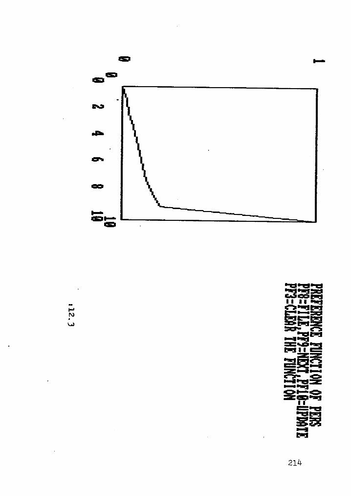
ausgk

cn u

cu Wk

|—•SI-•

·

•1:•-¤•-u

••(TX?]•-* r••-X

f=> I:-!|E•I!I¤·> $5*%1-„„¤•¤¤_|° "'·'ä'ä'llllltä%>¢•-I1-IIS

. •-1"¤1

EZ?--¤19*1=•-¤'”"§Staa•-1

. . Bl.!

21u

£ |-•

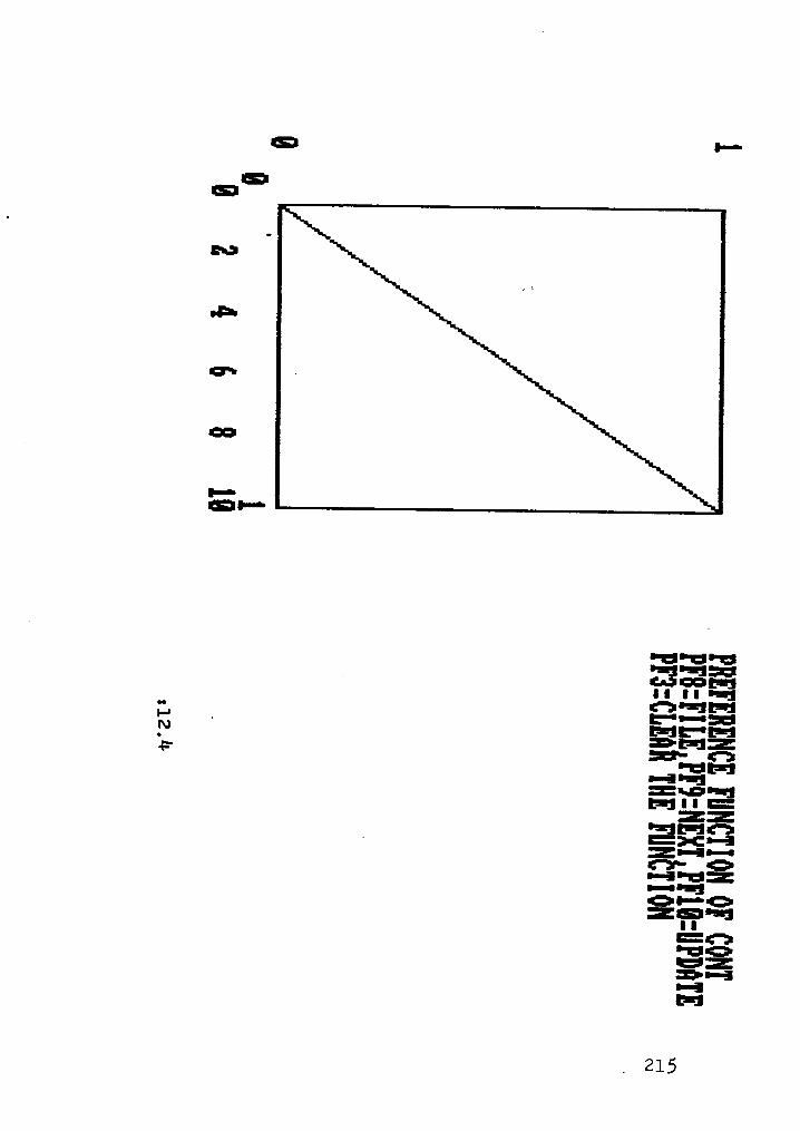
Ü

manga

cx

¤¤

pngQ!-•

•-¤•-¤•-51 'J>"""“"• • WQ„z Q2?N '

I!IE'°I!llr tlili"dg

•¤¤]|1q|tank!)Mää'ilälfä- iäucé.'1’•-i.•5•

$2EE•-1FI

. 215

I-

ä

mocs

cc I

•'¤•'¤•'¤

”925¤ gs;xn .•—i|q|

· M55äälüä><•-1

.iv-1S•Z22

I-·•-¤·

$5z-__]-¢·

In!

' _. 216

esma

uh- V

$5

_ ec

|¤-•

gn:

•·¤•·¤•·¤'lli¥?$··:„

Q2§"¤;°_, I!IIf"l!l~

?•—?’ä6$2

S2•-ZIEu

V217

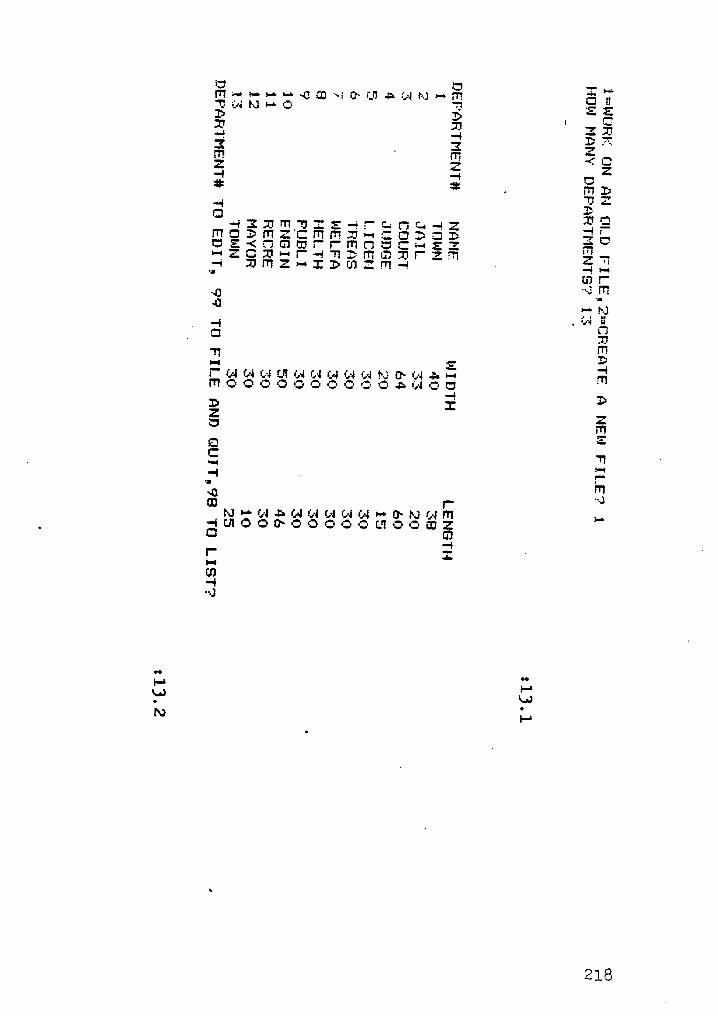
ij U InITI¤-··¤—~•-••-~!.7$~.Ir.1*~L!!s>=;-4Ir·-J¤-rI1 GI;13 L4 I*-J •—~ C= T! 5 59 9 I c1* J? am-!-63_ 3 Zm m <@Z Z Z-·I -6 gg;* * · EP,-6 _,—5‘*3 . . mo—III!V¤,'UI$.-Fäüäe-Z .gg—ITIC!bIT!ZI;'I'!1I'I'!3.*•-—•:I3.‘.¤Cb gn;¤‘E·<?J¤1G:I$'I"I'!'It'7‘·.Z„‘*C*-·£3' gn•-•ZGI*•-•I"—+‘I'IDI'¥'I=.E7!Z!I".‘.%¥7'I Zn-6 BITIZI-•I3>£ßI!'|'I-6 · -46-6

*0'J‘=

:-:*:2. ¤IT!‘¤

bT" L4 L4 L4 UI L4 L4 L4 L4 L4 9*-2 U~ L4 Ja •-•

g·n|'Y'|C·O·3·O·3·3·$-O·3¤=$=·¤*„4O¤—¢1>

ä IL

° "JEC TI ·. —\

p•••I —I"

~ß .._JU: I"|'·J•-•L4·¤L4L·4L4L·I¤>·4•-•G~r·JL·I!T'I »—6UIC·O0~C·=2·'3··C•·$·L'!·:··2·GZ‘

G G3-II' I ’

I-!U'!-6··~J

I-° I-•W noN I-•

218

:-·· Z:, 1 H C1FH E Z-:U] O E-6U') 1BTU'FJ :-6‘¤

CJ GD*-·· · Z T!:3 U3-6 UT!-6 I mmE Ü'!. UF'}

bmU] C Il'!7-6 T -6:-•D 5 IO1 FTD-·i TI 2-61-• ·-Q:-•ä‘

U3:6'!'T 2•.B .

- · ZT!I'-J UI!I! CÜ 2G1 :.1m ZDD äl!2-6 F!]. VU 17D Ü

TI2FT D7 E -6

-6‘T! ID»-• •-•I" !I!m *3

_ UT•-•U1..__}

llt

L4UI

z-: 6-•6-*

N P-'

‘ * 2lQ

G ~·^·- · 1 Ü U E ÜI! 1>=-·-—-·•-••—~-J¤J··~1¤I!—b'?=¤=;·¤?·.J-• :!'¥‘!¤1I!J·—1-• 1:1Z] 'T] '¥§ •—•4 -1 17 D D 4

I-U4 -1 -1 I•-•

M4 3 E -•D ·~„

H1 F'! DL"! Z Z AQ Q. Q Q. Q- Q. Q Q. Q Q Q Q Q 1.. 1-1 .1 .1

Ü C1 •—•3

1 xr Ce7.7U! C- C- C- C- 3 C- -12- -3 C- C- C- -L-1 ° 4:

*~n —{l 1:. 1:1C

73Z

C- C- C- C- C- C: C- C C- C- -3 :33 :1 -1.-1

C- C- C C- C- C- C- C- C- C- -~ 9-3 A Aal.;

C-C--3-C--C--3-3C--3C--3-3-3 U! ¤--—•-•

Q Q Q. Q Q. Q. Q Q _g,Q Q. Q. Q g„

A

C- -3 C- C- C- C- C- Y-J C- C- C- C C- xiOu

33'77‘C-C-C-C--3-3AOC··3·3-3-3 ID -•

C- C-EäC-OC-OC-·¤-L-J?·::1|j_J•·•-3-C-#_;• ~ü OU- UI C- C- C: C- D4U'!'IOC-C-C--1-4-¤C-C-C--’~1‘-C--C--3 •-·'E!C- O C- 'T!‘-0!|_I"C-C-C-•·•U!•·•-3C-·C·C-·C-C*-‘„Z- •-•

°° •-•|-‘Q Q. hb *·‘

3]PP .1I

OA.U1 P1-•11_ C- C- M L'? _'T!IiC·•·•-GC-C--3-3-2--3C--30-3

-· V'A H N'!

22-J

E'! _ O F: G DIn D•-·--•-·-*-GCD“~10'*F.I7-•’=•-.··1?··J-·· CTTFSWB-•-3 Z=;·19~J•-•C· .T'.·'¥3?·-·--9 ·x 7] D D -1FI'! __

IT! III!I!.--1 Z —s —1 J3-• 1T! -§ 3 E -—D < QT! D-•~ ‘~.-·'

U] Z A ·~C- G C- C- C- C- C- C- C- C- C- C- C- -· TJ—INV4 IT! A A vät C Ü Ile -« #1

1 Q

I! 1.*: =.‘I=m Q Q Q Q Q Q Q Q Q Q Q. Q 5;:} y.,} _

M -6 C-CJJZ

Q Q Q Q. Q. Q. Q Q Q Q Q gg ;·.__ggg

Q. Q Q Q Q. Q Q. Q. Q Q C Q Q ,3;n:.

Q. Q Q Q Q Q Q. Q Q Q Q. Q Q. L!} C C hg

C- C- C- C- -3 C- C- C- C- C- C- C- C- U- f

OC-C-C--3C--3--3C-C--Z--3-3 *1

"U1 9 1

Q,1

•—C-3-.--3-C--3-..--3-..-C--3 -...- -3 CB •-••^.

B.~ C.. ,..

- .. -"7C-C--..-„:-3-„-C-C--.-C-C--3-„- -0 Eef

-9IT!'I

C-C--3C-LH-3--C--.?C-C--3C--3 -;• T3-0_ II1*••

4:. :3: •:• ¤:• •‘:;1:} 1:: C- hb '° hr!•-•

·-·-··‘

uu1: -17 C.;•

I• .‘

Q CN 1}I:. •;• n:. x:. .:· e:. .3 aj .:« .2: ¤:: .3 z:. hb 11I-} CD

II· T1•-•-3 C- C- C- -3 -3 -3 C- C- -3 C- C- -3 -·•

I"L4 H1

221 .

1j _.^._

Hs

-•;__ _

f_ _ __ _

-. : -3 9, „*7 Z=;·iM·—•·3

1!'!JT3--•‘•

'<J3 D 3 -4U1IT! I!I!7JZ -2-9·D jaE E D

‘y‘

.Q; Q; Q; Q; ;:; Q; Q; Q; Q; Q; Q; Q; Q; 1-1:1V

Q NrZUäh ${T} Q; ;Q Q; .j Q; ;j Q; Q; Q; Q; Q; Q; Q; 1;,}1}} Q

Q;CI!Z

C- G- C- -3 -3 C- -3 C- C- C- -3 -3 C- L-!

Q; ;j Q; Q. Q; Q; Q; Q; Q; Q; 1- Q; Q; ,5.;“‘;

Q; Q Q Q; ;j Q; Q; Q ;j Q; Q; Q; ;Q Q!] I1 hb 1;,-}

. Q; Q; ;Q Q; Q; .:1 Q; Q; 1- Q; Q; Q; Q; Q;Q; __

-3*3-33-3-3-3-Q-3-*;.*--3'.'Z-C- ~J

T3__TI. -3-3-3-3·3C·~GO·30·3-3O Ü •;1;

?*·T.!-3C--3C--3\J-3·£D·30·3C--3= JJ g-1f!'|'I- *3C•·3·3-•C“-“3·3·3-3·3*3·3- •·•U-3 -3 TIr°. JP°° -3-3-3*3-3 L4 -3-33-3 C- C- -3 -•

°° -•!"‘

¤~ I-* 1]]PP -1

U

O ;·~OC!)

·¤C•·3C·C-·3C-C-C·C·C··3·3C= •-•TIhl ÜII

T?‘

1-•Q; Q Q} ;Q Q; Q; Q; Q Q; Q; Q; Q; Q; 1- g'-;-4 U'!

; Zgp;

Q ·^· , . 0:::-ra.«., I>•y•—•-•-;_•~G»Z¤~«¤~;¤-A¤„·JP-J-—gmg-1-ggg,.

·-~ Z-AhJ—·-..= 3131:-,·* < 1-:¤:>1>—6F'! T mzmmE ··~ Z-é—I35“ m «::~E 5 -.

Q, Q Q, Q Q, Q Q, •Q Q, Q, ,Q, Q Q, g.; · 2—@ITQAAÖQ

IT! -3 -3 -3 -3 -3 -3 ·3 -3 -3 -3 -3 -3 -~ 3-J #*A -I Q, -P‘·

.33Z •Q Q, .Q. Q, ,Q Q Q; Q Q, Q, Q, •.,,

Q ,;,4

' ·3 C- ·3 -3 -3 -3 -3 C- -3 -3 *· -3 -3 A

,:,¤:,,Q\¤:,,:,1j•Q5¤;\Q,:,-‘_j:,,:, L?} T,_!___=·

-3 -3 -3 -3 -3 -3 -3 -3 -3 -3 C- 3 -3 EP-

-3-3C--3-3-3-3C--3-3C-*3--3 *-1u

' U·30=33·3-O'3-3-3-3C--3--3- U3.

cl

LL- - - -.. ä-3 -3 -..- -3 ·...- O -...- O -3 C- -..- ·.- -3 ~ü g‘!>-4FH'I

-30-3-C--3-33-3-3--3-3C-O •·•*11 -Q, 1-,

. .8Il

..-- ..

-.. f"•• hb •• !_•

I-‘

"I-* U]4=' l=' -52-lI: C-'3-3-3-3·3·30·3'3C-C--3 •-•Q :g°

hl QIl

T U-3-~-3-3-3-3-3C--3--3--33-3 -·• r:-24 @11

2'2%

Ü ·^·L

. :1::::*:I1 1>-g--·-—-—~GC¤‘~3!1¥~L*¥-¤~ä:-ä?··J'·* CTHMZ---

;¤.«~H·J---3 :3*:313:-:-7% ‘äääääi. I1 z;:i“':%:Q -433:;:

A ‘ ' Q Q Q Q Q Q Q Q Q Q Q Q Q :.• Q~ -4 rf;.-„.AL$* G ¤¤~::

I '~•¢%

SU{11 :2: 2: ·2: Q: :2: :2: :2: Q: :2: :2: Q :2: [-_} ä ät

UI ·-·* Q· C

JJZ

:2: :2: :2: :2: :2: :2~ :2. :2: :Q :2: :2:.2::2:

Q: :2: :2: Q: :2: :2: :2: :2: :2: :2: 5

C- *3 -3 -3 -3 C- -3 C- -3 C- C- -3 -3 U! :-• :- g_n

-3 -3 -3 -3 -3 C- -3 C- 4‘·~J C- -3 C- C- 0*

-3C-C¤O·3*J-·3f~J•-•-3-3-3-3 \|

IT!A_ A

,A_A A 'W

-..C-·.·C--3•|‘Jf·~J•-•-L‘„•-..-C··.- Ill :-•

EAA A A A T?·‘3OC··„--..·hJhJhJ-„·O-4-3-3 ~O 5

3-4I"

-3C·“30l-JC·C--3--3-3-3C--3 —· #3*3 TI

??Q•• -3C-C--3-3PJ-C·C·-3*3-3-3-3 •·• •• L:1- -·

:-• ugP P -4

• • • 'I

{S :2: :2: :2: Q :2: :j Q Q :2: :2: Q: :2: •j IdI-J

Q¥:

C··3-3-3-3C•·3C--C·C“=-3-3-3 -• F:L4 m

22/«>

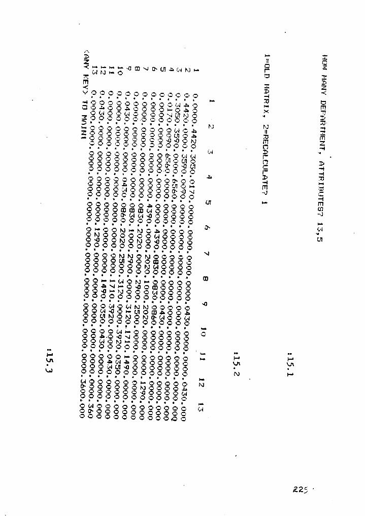
-—IQ4 43ä

CZ E<-•-·-—-~—fJ¤2‘~¢0—L-I-é¤=;··44-J-— I'- „¤}=i4'·-J•—-C- 52R1

=- +{

D -1·,- Q Q Q .·~· Q ;·· Q Q Q Q Q Q -. -4EI.-! I rl Hr'! I I II.?

|¢-.4 Q Q Q Q Q -·-. Q Q Q Q ·;.,; „,·; Q •-4.G-3·¤-3-3·$•-3-3C--3-C-~•'=•-3X-3-}-4 C- C- -}-4 -3 -3 -3 -3 ‘-~4

UI 4*-J C- ° ä3 Q Q Q Q Q Q _QQ Q Q Q Q Q .·.=·

:>• • 1 1 1 1 1 1 1 11 1 1'Y*·• C- -3 C- C: C- -3 -3 -3 C- C- -;-4 -3 b H IZ Q Q Q Q Q Q Q Q Q Q U; Q Q E T4'!. ..1 Q Q Q Q Q Q Q Q Q Q Q M FT}Q Q Q Q Q Q Q Q Q Q Q _ U -•I

I I I I I I I I I I I I I;;_•j

'· •-3 C- -3 C- -3 C- C- C- -3 0* -3 -}-4 G4 I--3C--3-3-3--3-3C--3iü-C-L4'4-3 Ü 9C- C- C- -3 C- -3 -3 -C-C-3-3-0Lü I: 'IQQ Q Q Q Q Q Q L':1.r:«:¤r:'; Q 4" -4I I I I I I l I I I I IIQQ Q Q Q Q Q Q Q Q gg. Q Q -4 •-••:1.:¤ Q Q _;Q Q Q Q Q Ln Q 4..IT!C-C- -3 -3 -1.4 -3 -3 C- -3 -3 0* ~0 ~4 '*-I ‘-

C-C--3-3-3-3-3C-C--3--3-'3-3 “II I I I I I I I I II I I Ln,1·C--3·30·3-C·C·-¤-3C‘C-C-C-

U4C-C-C-*30~¤Q4-„·4~0-3C--C--3 C-C- -3 -3 C- -3 C- C- C- C- -3 C- -3 -3 °T‘I I I I I I I I I I I I I } Id:} _-3-·-•·3-3|~J•·|-J·3-•¤•-3C--3-C-

"„·34~J·3C·C- -3 -3·3¤}4C·C- -3 C- I·‘-C-~0C-’3hJ-3t-J*3~i3-3-3-3-;--3-3‘3-3-3-3C--3-.--3-„-·3-.-I I I I I I I I I I I I

IO-3-3-3hJhJ-34-J3C:3~3-3--3-3Q-3gI0OO@OQ-3-C--3C--.„--3-.·-3-3-4-Jß~|C·-3-3-3-3C-C--3-30-·.--3-3'3-.-C--‘3I I I I I I I I I I I II-3-3-•-·•-}4-34=J•·•-3C-C‘*3-3· C-C--¤~4»—O~¤-1*EIl-3C--3C--3-3~£|•·•*—J-3-3--3-L4-3C--l“--3-1.-O-„..--3-C--3-3OC--C--3-33I I I I I I I I I I I I I -0C- -3 -3 -}-4 -3 -}-4 M M -3 -3 -3 Q- C--3-3-1-4-0-3-·L-I-3-üJ·4>-3·=„_-gb-30-UI!-J-34-J-34·J0~-1-4-3-„e-,-4C-C-C-‘3-3C--3-3C--3-3-1‘--C-I I I I I I I I I I I I

I-3-3C-OL·4-•-3-3C--3-’3-3-3 C--3C-g¤—-;_‘-~0*~4-3--3-3-Q-C--3-.3-3-3-..4-..-r·J•-•-3-2,*--3-C--7.*-C--3C- -3 -3 -3 C- -3 C- -3 -3 -3 -3 -3 C- .gg I I I I I I I I I I I I I i

·• ••I- C-C-C--ZZ--3**-3-3-3-3-3C‘--3 ¤ I'° C;Ux -3•3C-ä¤}-4-b3-3-3-3-C·C‘-3- En ,•

-3OC-·3·4UI~0-3-3-3C--3C--3hl -3-3-3C--3-3-3-3-3-3C-OC- N I-II I I I I I I I II I I I i °ß-4-3-3-3-3-'3C-*·•C-C-~3C-C- P-J0**-3-3-OC-O-C-P-J-3-3-GO-Ln-3C--3C--3-3-C-~0C-C--3-;‘j-}·4-3-3C--3-3C--3-3-3-3-3-„--3I-I I I I I I I II I I I piC- 4}-4 -3 -3C--3 C-C-*3C--3-3 C- -}-4-3Q_*-3C-C-C--3C--3C-C-C-G-3-C--3-3C--3-3-3-3-3-34C--3

22“‘J

#*1xr-:-•' · 1'·¢••·¢¢1¤

Sd§•'¤•¤¢§|wvzr

2•·—1G1.*7gta?.2*

F!EEG ä·—·-

2%

·‘

£••-•|-•l-|-••I-••—¤X-„1¤*•§|1;§•tn§En'II-~i&*>t¤¤hJ•-£

•-¢•-iVäiI5!lt')

xr •¤•tnJ¤¤¢JI•¤•t¤„¤!~•>I-••§•ta¤J!•¤.'II·-•£ I-•

ät¢¤•‘€

¢')•-•t¤¤IhJtnJ•„¤•t¤¤¢¤J|-•l‘¤:tn„:I·¤:n|-~£|- hä

•-•

1 I5Jt¤:•¤•tn¤I'•§I-E¤Jt«¤>!~JI-£l-•hJ ta:EI

ta¤•§§I'I|h§I-•I‘~Jt•¤J•h•l-·•£I-•·!~:ata¤J •§¤

•„h•§|'I¤'•|-~I·~Jt¤•J•„§¤LI'I£|-I„¤n:t„••J•„§• LI'!

t•:¤¤I·-•.§tn:hJI-~£LII•§t„¤•:aI„'u°aI·-·~ ¤*~

’hJI-•!••Jt„¤¤!¤3I¤-•£I·-••§t••.I!~JI-••I'.‘¤: ··-J

h:t•:•§••-£l·-•¤•¤.:t•¤:•I•~•:a•-I„*~„:>t¤:••¤• an

ERJ tn§•h•§I'I£I-•I'¤Jt¤J,¤¤I-¤¤t¤§•§¤L|I I-•

hn)!-£§I'I•h•t•¤>I§„3I-•¤*~§II•§•t¤J¤•J I-

I-•{I-•g}¢é§JI¤¤*!'l3$l'I•«}¢¤§El§¢nJ I-

£|-•I'•'•¢tnJ¢¤¤I¤-•E¤„Jta¤J•ätn„II*¤Jtn:•§• F-

' 227

1:CONSTKNCTION RONTINE #12:CONSTBNCTION RONTINE #23:CONSTKNCTION KONTINE #34:NEN BLOCK PLON 15:INPROOENENT NONTTNE6:P#IRNISE INTEBCNONGE?=DR#N THE PLON OND COLCNLOTE TNE COSTB:BOCK TO LATONT CONSTKNCTION NENNSELECTIONN? I

,21.3

1112 1 4

222; 2.662261CONT KEN) TO CONTINNE

:21.4

··"·~4'Z'4'!'f‘4"4'|"4'4'4"'4'4"?11 -·^·-4'4"4"f"4"4'Z"?'T'4"!'§'4"??7DOGGQOOOGGOOGOX Z>OOSOGOOGGÜCOG><

NOGGCGOÜOÜODÜD-•fZZZZZZZZZZZZZä ·<ZZZZZZZZZZZZZ§°s J

4 Q •-— 4=J 04 U 4 ¤1··4 hl •-— O GG G C Q

Z 413 ' ua 73 ulVUUUUUUUUCUUUUU4 NUOUUOCUCCGUUO-4

ZJJZIZIZBIIZIIYI4ZZZZZZZZZZZZZ

ZZZZZZZZZZZZZ

Z•·*

N Ol O 4 Z C- 4-J •.„·6 •-• 4"‘

Z "* Zm 4T!

äh S?W

•-•

13 'U, r- VITI . m

ä äm U1

4;g-• Ill

-4 · -4

O OZ · Zwo 4-*G O

_ 229

O-4 GZSZ?G7

E."73?T‘}‘I] ?UC.'1$J?F

js}!EU!U"

, ‘·•Ü

-6-· , —-QCGZJCJQu :azI-*3-4

4 —§=L„~1¤L-·}C*CC

Z Z Z*3—é -}

O C •—•

Z ÜI> •-·

·•-6 1-•

ZZ

E} Üs-•

E} i !!. '< •<

F'} F']; U3 _ LE

Ü 4 W

Ä PJ l'=Jll ‘ Z Ii

3 Z · ZCJ-• D '¤vl! .-

T!..__} .._J ,,.,"‘O

-1 Hs-•

—I

Ü 1}- C3 3

· . •—r··« .gk

7]I!

••

I-4_D "U

I-*

230

HELPNENIIPF1:HELPNENN

PF?:CHHNGE DEPHRTNENT SIZESPF2:NOUENENT B9 1 0R 19 DISTHNCE NNITSPF3:EHTER 8 DEPHRTNENTPF4:RENOUE 8 DEPARTNENTPF5:RECTILINE8R DISTRNCES NHTRIHPF6:B8CH T0 LRPONT CONSTRNCTION NENNPF9:ROT8TE H DEPHRTNENTPF19=NPD8TE THE SCREEN ~

DEPT8 NRNE HIDTH LENGTH9 8 199 1191 TOHN 4 382 JRIL 33 293 CONRT 64 694 JHDCE 29 155 LICEN 39396TREHS 39 397 HELFH 39 398 HELTH 39 399 PNBLI 39 3919 ENCTN 59 4611 RECRE 39 3912 HAYOR 39 1913 TOHN 39 25

DEP8RTHENTR,HIDTH,LENGTH? I :22_2

231

1 16 111311 I

IN l

1ALT.#1

232

° 113 711¤

nä111

l— «A1.T.#2

3

233

" l Ü]1 13ZBLL

1312 l

ll--lü 61

:ALT.##

235

LJ.I,

;ALT.#5

113 111ll

N:ALT.#6”

237

7% 7?%£•-• Ex-•$2 E- 2Xu: XEEhtm: ¤¢I‘.=¤:I|-•·

65n ·¢·•—• nit!)

Z- •—••·¤

I¤¤§ 65¤¢•¤•5-2651

A EE?TE _ T"?|_¤_1:¤· I!-'.I£·$•·

II ' II nv.:65*EI ¢'5 I-'¤•"•'Iii EEli EI U!265

=¤• c":nänä U-! E-p-:|•—• t*.l E" ·

E *"::5-2 zu äE? E «-„Ei E Eurg;

•!|G6•¤-•§ •¤¤• hä

E'65 . IZ" E!¤:I•-•ÜE

E

_; _

°' ¢'5 ‘~•*13 E MJ .*·‘ FS >-·

EE2-

238

Gü I-!2

•·¤

E"U

ägIE-EIX2ll-!

ii¤'>•äX:„=S""’

· •-F4 «.«¤¢· £Ä

2Ä

1"U¤$••—l22rs': I—•EI 1_ 1

. I-•ää

S"-?£I-| | 1ll q

·

.U9 Inn;i" ¤r••-¤N Bilé .

ES_ Fa i EIh: I-~

I I I II-

239

an "“

ä

cu

4:.

¤··„

cn

E--£ E

‘ •·¤•·¤•¤¤¤:l

EEQ,•-ngrvIr•I:=:I·IF-I1N·• fü•·_;n-lisa

EEE-Elli':·_ :-:-41"‘-'S

-;:2*.:;,.*3$2$$0 3*EI

240

ÜÄÜ\\

,¤„ \*

¤~·\‘°°•

¤¤jn

äsngk:-••lan~§kä-•¤ _

"¤"¤'lli' X?

I I •¤¤_|C, 'ältlN nnni

- . FWF!xn Edi

' ‘ Eää!¤äI¢"‘:>C•ä•ä•¤-•1 T-uä°=||-•·-2'5‘”'—'il-!"¤•'¤

· $11-•-I[EI

_ 2l-I·l

2L3?-._;a_;·;>Agj

EINE,.

E

NE6

$’¥„

JEg?

+s§{.¥6‘”J+?};;~.

E-‘5Ni

*2**2:i

C2

Em?1;

E2-

E

gf!

Bj:

+5

—.=‘ä1

cgj:7;::~·L7_5

2

mv

ZZ;

ig

"‘TE,'

1Z

-5v1“

Z

*€*<:2

:

zä

Q1Q

2ä

2

IN

,FE5„F„

’FI

$„

4,

1

„;·'»•_•3—¤Q?u;_'

?

;

_<

·

gd

J;

12-7

.

3

2

äN

E“

2

ä2

$2

1

'

2

.

1._

:.:..-

g_

Fi

2

I

I2

2

E

2mn

„ 2

2

2

-N

Er

2*--%*

E

{

{

-

1:-

""‘ t

I

=

1

S

2

1

QS

<:

2z

i„-, F

I

-.2-

STI

I

I

,I.

I

?7

{

--

5-.1,,:1#3

E

1

5

*—•{

21+;

“°I

1é

Z6:.-:

SF2

I1

5

1

.

{

·,.„,__

6

E

Ü

3•-•

I

1

E

Q"

2.2

5

ig?

~,:‘. ä

ä2

3

I?¤§I

E;

wb

U,,

1··'· X2

z

2

‘·

32

Q2:3;

2

2

@2

,8C3* °

E3*

’— v *

é

1~7

21-~¤=:

‘

‘·

3= 3

2 3

;2

2

*3

{”° 2 fg

E ii

¥?·—¤§

2

·’

f

{

1""'

1

T

6

'

»X

U3

1*3

IG1

+>

m

„

.

.

1~ü

5

.

5

Q'—

„1

·

2

2

w33

*5=

v

10

1~=7

2-

•

-1

(I.;Ü

5

I"

Q

J)

NZ

Q

5

Q#3

*1

2113,.

{C-.,_L¤‘;

2

5

~;-

Lau

1

1än

• U{5-

?

·

1-•m

{¤‘•~ iqÄ

I

2ä

P*2%

2

·~;

1

’ m1....

„

I‘1M?

1P?

1

1OG

{

n

••

6

\J

1

ko1-*

9

ZD2?

-

.

15

' 4•-4

ß

6Q

De

-

päß-E*6

-:6;-

·«

.6.¤—•r··%"-‘

mil

.4

1

I!

"1

-¤

..

.•

--

·Ü

— I PO.r

e. e.; .-an '·.

„ -. 6 ~

Q

—•-‘&;¤n:.1;

_‘~¤-.L*···—;·3:

*

<' . ·-= "

. r;- - ~

‘

—•

_.EÜ-6

vdmgqq°°°-*

n

Qt

‘·J

-5_7 111

-6·

'·

.-

ar . . T 6~·€ · ~

4

._¤ fn

#{4

_-Ä -*7,„•

1.-_;¤_;

1f

ä

4?66:

F2

_

‘

...- E{J S.} "

·•s

Q U, Q-

-, . 7q

-w

4

a

Ü.! ·°° ··.'&Q"

"'T

. _;

_

1 Üw

''

¢»

-

C:·'

QJ 2- 11

"-1"-

*‘ =l%6-•

4I

4

‘; w' ~!~

·•n._j

2--

~

QT!

"" Qu_;

—

4 v .3 .4,

FPÜ

. :7.

QQ

3 626::

.6-

__..

_, ‘.. I! ;>-_?

?#

1

V4

2 -

66

°

E

§ o -

1

B

I)

'°‘·-¤‘ ht

-s-

—§

54

‘ 77

P1_°

1

'~,• n:

‘_

Ü}

-

é

••J

4]

t

—·

.§‘JT?

.

5

vv

"

Ü-2V 5

a, 2

E

• .4 -0 B

3},

:

L} • \<

z.

ä -*3

:

Q3 ,0

T""°

.,4

7:G

s:w -

_..-:1

-7

4·

.~ *= 1

-,g G

gg.; '

::;_

nn

§=

_;- ".;

1

Q;

-.¤‘

••

'_ »'«

no

'§

1

-»"

°¥;

F

u -

· ~

“ 6

-

” Y” m

w

“

· »

;_, =ET ¤~ Ü

€¢

.

é.:„ C-

•_•

_;L ,-_ LQ

_,

Ai

¢ "' "-. 1*

7_ PiL;

,Z

».„ ' _ nv

r-•

a

*4-1}

·:

-¤•

‘ ,0 .

6V'

*1Ti

S;. ,;

·=‘·

Q:1:1E ZZ 112 1

äz 1 ;;=1 Üzwz Qi1 ".• f

-- ·Z"!Ü;

#<..]]i :#«f§1]1 gg-·'·;11 $1.,-@1 mm? mm: ääi E:5 ¤$•‘¤·~CE #{5

F4?grzvjv

r.-11111131 1- S Y" "" :3 i Ä:*

-• _ä

:I |l|

'Q1 -11 -16I1 :2 :1 -6.mr

1 F4 Z

*6 •= 'Tli 7115mf

__Q !11

**11

gzQ1

‘ E P 1 "21 :1z1 mä'111 § II 1 rr

··’

-1! -11 'Ü! lfji n Q: 1 °

· - G! •I .ze az: urz: F"J3! „.

3>. *4;•Q-71*:1-I 1.111-1: 211.,; ..r-! BZ! *2} ß·1z1 4*.141 1,-J.1:1··Ji

7 -131 v1.„.11 7 1 1 2—··-· *-1 ..··u1-1

)( „ß Q 1:1 I )( I 1:1 1 I ><1 —1 1 2 E 11* s 31 ~¤ 1 41 S ~ 1 .1 16 . '31 , Q1 11 1 3 1 3‘ ··=. 1 * Q

1“° S *° Q 13 1 ~1:•

Q Q 2 S .. l *! E 1 1

· F ' 1 :1S '·Z' C2 C· ·2·

P 1 1 1-: 1 -1I'

•

N

. II

2L1L:»-.

Z-'>I- E-6

Z ·_. I

6*-.;ij?}

$7

B2)

77

E

I

7

..I

-1~J

I .

F°I"2

E.,

•_ ,

.1·

1

··

1

;_

:2

2;*52

¤‘2l*·

2"¤,..¤„„

.

7

'

•i

:

•g.

:E

*,«;ä·«

2m

...2

Zi-Jzjf2

,;-6

6:6i

4*

2

Tag

Tx

5

*777

¤

<:

‘

‘

-77

Q

_. e-[T' -

‘•'! 6

q.

ä

•-‘

_‘

gTI~_, I

IJ;}I

_; J

-. 2

,.

j 5;

‘; 2

·=-...;=,;G

I

2·2I C:

.I_,

„,

2:: Q,2

•·_. .;;

=

.

TJ

nu7

••-•7

2-1Z?

::‘·"‘Z*·**i"2.._

*-*112

2**

L: 2

rn ;

“ T2-2

,5

-•"?-'TT!

2

·»2

-32-

2 g.2,

rä

‘

.-1

*72

.„ =

·= =

:2 ·1,

··-·-Ma,2

:2:

A.,i

6-'• ;

J

"i

;•~

mf

5;2

I-6- 2

2-.

2,2-

—é G

rr? =

‘

7 2: 2 9;*Z

-6j-

__

.

,£ ·

. 2g.

-:;3,.

:I. *~.- -

7.3

‘= 2

Z¢ ·-·

‘·—‘

7A.'

7:*:7sA

:•|?

J

-*7

Z7

°··•,=':rn

-

=·—

¤— 2

G'!

2

Z;.}E

2

‘

—I 7

E -E ...

7 ·

I

-•

A_„

§

L'.;

.

Ä

;

‘

é—·2

222

I

§

Ü

*

,—

_’

,..3-Z2I;.}

E

";’

2*:7,._

;

·-2.i

2

'J E

A;

ÜI?

7

Ei:7 '7I· -

—•

-

__ {Z

·'.';_ ·

§·‘4 „

*i‘ 2

Z Ä

x7-*

_I6§

..>·

‘

:2-=

Ü:3*

F6

Ü

7

CH

t

ä

I-!

*

*43

° L-„-

5..,'

,- g 6

?‘

‘•' I

Ü ._

·

G~+‘J

E

-6-=·‘“°

gä?

Ü;

7Q

“·_,

'°:•.

77

6·

‘

_*

*'

_1

• '

7-11

"i

·;Ü

"}

:

_;

v

!

••

I

~C

'

Xi

‘¤ {9-•

7*:,

°

F

G*'

2

nä-6

6

'E!

T

'._.

ä

._

6-I

m2

=

,

··U.

I*·Ü

.Q

2

~..

,...

9

•

I

,_

(

I?E

'

2

.J·2

"*6

12

.

}

’>

APPENDIX C. RANDOM MATRIX GENERATOR

Program to generate random matrices is shown in this appen-

dix. These matrices are used for testing performance of

CORELAP and the proposed procedure.

10 REM RANDOM MATRIX GENERATOR20 DIM P(25,25)30 INPUT "NUMBER OF DEPT. AND FILE NAME";ND,N$40 RANDOMIZE : CLS50 FOR I=1 TO ND60 FOR J=1 TO ND70 IF I=J THEN P(I,J)=O : GOTO 10080 IF I>J THEN P(I,J)=P(J,I) : GOTO 10090 X=RND*10 : P(I,J)=INT(X)100 LOCATE I,J*2 : PRINT P(I,J)110 NEXT120 NEXT120 02214 N$+".DAT" 202 0u'1·2U·1· AS #1140 FOR I=1 TO ND150 FOR J=1 TO ND160 WRITE #1,P(I,J)170 NEXT180 NEXT190 CLOSE #1200 END

Appendix C. Random Matrix Generator 246

by pasu“loharjun0 - vtechworks.lib.vt.edu · generated by corelap. dedication this work is...

Documents