Turbulent Mixing in Stratified Fluids -Layer Formation and Energetics

By

Young-Gyu Park

B.S. , Seoul National University, Seoul, Korea, 1987

M.S., Seoul National University, Seoul, Korea, 1989

Submitted in partial fulfillment of the requirements for the degree of

Master of Science in Oceanography

at the

~----- I MARINE BIOLOGICAL

LABQRATOfN

MASSACHUSETTS INSTITUTE OF TECHNOLOC Y LI B R A R Y

and the WOODS HOLE, MASS. W. H. 0 . I.

WOODS HOLE OCEANOGRAPHIC INSTITUTIO~-,-_...J

September 1993

© Young-Gyu Park 1993

The author hereby grant to MIT and WHOI permission to reprodu'l!~

and distribute copies of this thesis document in whole or in part.

Signature of Author ---'-{M7f-"--~---:--r--~-r----:r--~--~-------r U tJ f ~ to J~int b P/o1 ram in Oceanography Massachusetts Institute of Technology Woods Hole Oceanographic Institution

Certified by ~~~----~~·-· ·-<~~~~~~~~~~-----0-r-. -J-o-hn_A_._W_h-it-eh-e~ad

Thesis Supervisor

Accepted by ~-'-'_;,_ ___ _ Mr-+'----+----------------~ v Dr. Lawrence J. Pratt Chairman. Joint Committee for Physical Oceanography

Massachusetts Institute of Technology Woods Hole Oceanographic Institution

Turbulent Mixing in Stratified Fluids

- Layer Formation and Energetics

By

Young-Gyu Park

Submitted in partial ful£.llment of the requirements for the degree of Master of Science in Oceanography

at the Massachusetts Institute of Technology and the Woods Hole Oceanographic Institution

September 1993

Abstract

A turbulent mixing experiment was conducted to observe the dynamics and the energetics of layer formation along with the region of layer formation in the Reynolds number (Re) and the overall Richardson number (Rio) space. A salt stratified fluid was mixed uniformly throughout its depth with a vertical rod that moved horizontally at a constant speed. The evolution of density was measured with a conductivity probe.

As the instability theory of Phillips (1972) and Posmentier (1977) shows, an initially uniform density profile turns into a series of steps when Rio is larger than a critical value Ric, which forms a stability boundary. For fixed Re, as Rio de­creases to Ric, the steps get weaker; the density difference across the interface and the difference of density gradient between layers and interfaces become small. Ric increases as Re increases with a functional relation log Ric ::::::: R e/900. The steps evolve over time, with small steps forming first, and larger steps appearing later through merging and decay of the interfaces. After some time the interior seems to reach an equilibrium state and the evolution of the interior steps stops. The length scale of the equilibrium step, 13 , is a linear function of U /Ni, where U is the speed of the rod and Ni is the buoyancy frequency of the initial profile. The functional relationship is ls = 2.6U / Ni + l.Ocm. For Rio < Ric, the mixing efficiency, R,, monotonically decreases to the end of a run. However, for Rio > Ric, the evolution of Rf is closely related to the evolution of the density field. Rf changes rapidly during the initiation of the steps. For Rio » Ric, R1 increases initially, while for Rio ~ Ric, Rf ecreases initially. When the interior reaches an equilibrium state, R1 becomes uniform. Posmentier (1977) theorized that when steps reach an equi­librium state, a density flux is independent of the density gradient. The present experiments show a uniform density flux in the layered interior irrespective of the density structure, and this strongly supports the theory of Posmentier. The den­sity flux generated in the bottom boundary mixed layer goes through the interior all the way to the top boundary mixed layer without changing the interior density

2

structure. Thus, turbulence can transport scalar properties further than the char­acteristic length scale of active eddies without changing a density structure. When the fluid becomes two mixed layers, the relation between R1 and Rit was found for Rit > 1. Here, Rit is the local Richardson number based on the thickness of the interface. R, does decrease as Ri1 increases, which is the most crucial assumption of the instability theory.

Thesis Supervisor: Dr. John A. Whitehead, Senior Scientist Woods Hole Oceanographic Institution

3

Acknowledgments

Thank Dr. Jack Whitehead. He is more than an advisor and his guidance and

encouragement made this thesis possible.

Karl Helfrich also encouraged and helped me to set up the equipment. Glenn

Flier! guided me kindly. Comments from Ray Schmitt and Rui Xin Huang were useful.

Anand Gnanadesikan and Jack Whitehead gave me the initial idea of this work

and discussion with Anand was helpful. I cannot forget friendship from Joe LaCasce,

who is my only classmate, and Bob Fraze! in GFD lab. Bob also helped me during the

experiment. Abbie Jackson in Education Office teaches me English.

I also thank Korean Government who gave me a chance to study in US.

It is dedicated to my parents in Korea.

4

Contents

Abstract

Acknowledgments

1 Introduction

2 Theoretical Background and the Experiments

2.1 Theoretical Background

2.2 The Experiments ....

2.2.1

2.2.2

2.2.3

The design of the experiment

Apparatus and procedure

Data Correction .

3 0 bservations

3.1 The evolution of the density profile

3.2 The evolution of the interior layer .

3.3 The merging and the decay of interfaces

4 Analysis

4.1 The length scale of layers and interfaces

4.2 The spectrum of the density gradient

4.3 Energetics .

4.4 Density flux

5 Conclusions

5

2

4

7

11

11

13

13

14

17

20

20

29

31

34

34

35

38

48

54

5.1 Suggestions for Further Studies

Appendix 1

Appendix 2

References

6

56

58

61

62

Chapter 1

Introduction

After the invention of rapid response themistors, ocean observations have shown the

widespread occurrence of microstructure in the density field. On occasion , a mi­

crostructure is in the form of a succession of layers and interfaces. The density is

almost uniform in each layer and jumps nearly discontinuously across the interfaces

that separate the layers. Since the direct measurement of any vertical flux is as yet

technically difficult, the scalar microstructure has been used to estimate the turbu­

lent vertical fluxes of some scalar quantities such as heat, salt, and density. But the

energetics, i.e., the conversion of turbulent kinetic energy to mean potential energy,

of turbulent mixing in stratified fluids is poorly understood and the estimation of the

vertical fluxes is based on models, which do not include the dynamics of microstruc­

ture.

So far, most laboratory turbulent mrxmg experiments have focused on the bulk

transport across interfaces (Turner , 1968, Linden, 1979, 1980). In those experiments,

two mixed layers with a sharp density interface between them were prepared in a suit­

able tank. Turbulence was then introduced in one or both layers and the evolution

of the density in each layer was measured. The mixing efficiency, R1 , was parameter­

ized using external parameters such as the Reynolds number , Re, and the Richardson

number, Ri, which is the ratio between potential energy stored in stratification and

available kinetic energy. The experiments show that as Ri increases from zero, Rt

also increases from zero to a maximum, and then decreases as Ri becomes even larger.

7

These experiments have been useful in determining the mixing properties of stratified

fluids with fully developed layers, but they may not be appropriate for describing the

mixing properties when layers start to develop from a uniformly stratified state.

Those experiments also cannot answer under what conditions microstructure oc­

curs. Phillips (1972) and Posmentier (1977) .developed theories for microstructure

formation. A statically stable uniform stratification may be unstable to turbulence

so that turbulence breaks down a uniform stratification to another structure, a series

of layers and interfaces. The most important assumption of the theories is the rela­

tion between R1 and Ri. As Ri increases from zero to a critical Richardson number

Ric, R1 increases from zero to a maximum. If Ri increases further beyond Ric, R1

decreases as shown Figure 1-la. If Ri of the initial state is larger than RiC) turbu­

lent mixing amplifies perturbations in a density field accompanying a change in a

density flux or mixing efficiency. The density structure stabilizes while evolving to a

succession of steps.

There are a few laboratory turbulent rrux.mg experiments focused on layer for­

mation. Ivey and Corcos (1982), and Thorpe (1982) stirred linearly stratified fluid

with vertical grids moving laterally. A series of turbulent mixed layers intruded into

the non-turbulent ambient fluid away from the grid so that a step-like structure was

generated at the outside of the active turbulent region. Thorpe (1982) tried to relate

the step-like structure to the local instability theory of Phillips / Posmentier, but he

could not verify the theory. Ivey and Corcos (1982) showed that the intrusive layer

was due to the collapse turbulent eddies in stratified surroundings and the intrusion

made a negligible direct contribution to vertical buoyancy flux so that the intrusive

layers could not satisfy one of the necessary conditions of the theory.

Ruddick, McDougal and Turner (1989, RMT afterward) stirred salt or sugar strat­

ified fluids horizontally with an array of vertical rods throughout the depth and length

of a tank. The initial linear stratification evolved into a series of steps when the stir­

ring was weak and the steps disappeared as the stirring became strong as the theory

of Phillips/Posmentier predicted. Until now, RMT is the only experiment that ex­

amines Phillips/ Posmentier's theory. But RMT was an exploratory experiment and

8

0

,__. layering regwn

(a)

Density

a convergence

a divergence

(b)

Ri

density flux

a uniform initial density gradient

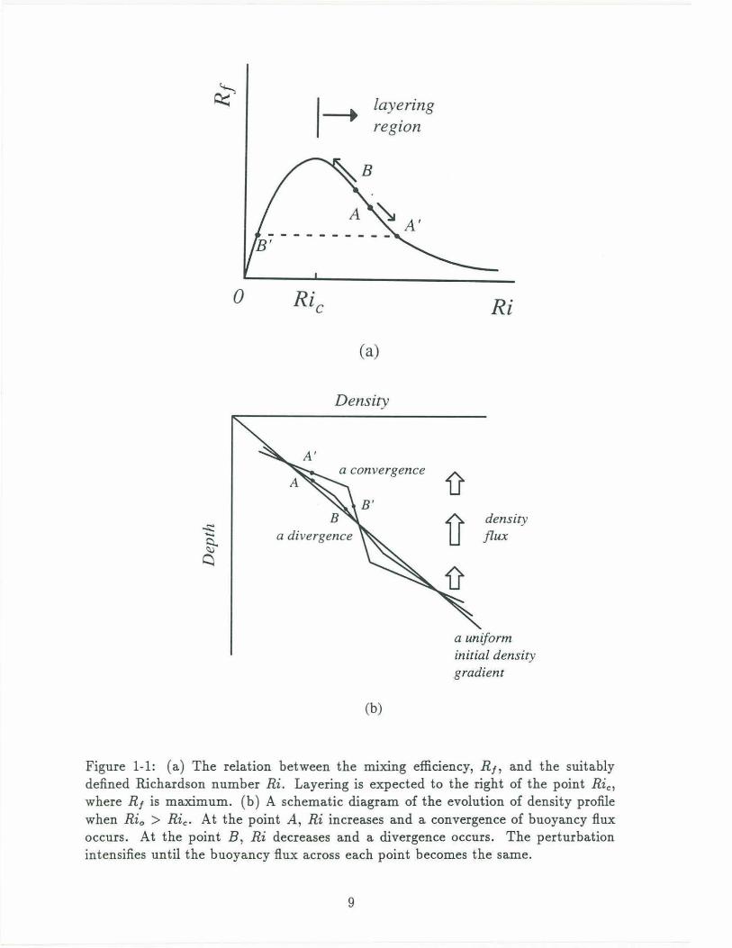
Figure 1-1: (a) The relation between the IlliXlng efficiency, R 1, and the suitably defined Richardson number Ri. Layering is expected to the right of the point Ric, where Rt is maximum. (b) A schematic diagram of the evolution of density profile when Rio > Ric. At the point A, Ri increases and a convergence of buoyancy flux occurs. At the point B, Ri decreases and a divergence occurs. The perturbation intensifies until the buoyancy flux across each point becomes the same.

9

many questions remain unanswered. Among them the most fundamental questions

are "What does the stability boundary look like, in other words , what is the relationship

between Ric and Re ?", and "What are the energetics of layer formation ?" .

In the present experiments, an almost linearly salt stratified fluid was stirred

uniformly with a rod at constant speed until . the fluid was completely mixed. The

evolution of the density profile was measured with a conductivity probe that has a

resolution of about one millimeter. A linear motion system was used to control the

mixer and the probe so that it was possible to get accurate control of the rod speed

and estimate potential energy changes of the density field. The energy budget was

used to investigate the energetics of layering, focusing on the difference between the

layering and non-layering cases. Since the fluid was mixed until it became almost

homogeneous , it was possible to relate the mixing efficiency and density flux to the

evolution of the density field. Finally, by changing the stratification and the Reynolds

number as widely as the apparatus allowed, the stability boundary for layer formation

was found.

In Chapter 2, the theoretical background is discussed. The chapter also contains

the design and procedure of the experiments . In Chapter 3, the evolution of the

density profiles depending on the parameters of the experiments is described, focused

on the evolution of layers and interfaces. The stability boundary is also discussed in

this chapter. In Chapter 4, the length scale of the steps is discussed related to the

external parameters of the experiments. The energetics of the layer formation are

also discussed related to the evolution of the density structure. Chapter 5 contains

conclusions and suggestion for further studies.

10

Chapter 2

Theoretical Background and the

Experiments

2.1 Theoretical Background

Phillips (1972) and Posmentier (1977) proposed similar hydrodynamic instability the­

ories for microstructure formation. Far away from boundaries , in the presence of

turbulence, a linear density profile may be unstable to small perturbations in the

vertical density gradient, if the stratification is strong enough or the turbulence is

weak enough.

The theory is based on the relation between the flux Richardson number, Rf, and

a suitably defined Richardson number , Ri. They assume that Rf increases from zero

to the maximum as Ri increases from zero to a critical Richardson number, Ric. In

addition, R1 decreases as Ri increases beyond Ric as in Figure 1- la. Physically, if

Ri > Ric then turbulence is suppressed and turbulence cannot mix a density field

effectively. If Ri < Ric then turbulence is active, but there is not much density

difference to mix so that turbulence ·cannot mix the density field efficiently. If Ri

has an intermediate value, a density field is most efficiently mixed. Now, assume that

initially there is a homogeneous turbulence and a constant turbulent vertical buoyancy

flux throughout a uniform density gradient. Let the vertical density gradient be

perturbed locally as illustrated in Figure 1-1b. Ri is increased where the vertical

11

density gradient is intensified (point A), and decreased where the density gradient is

weakened (point B). R1 changes in response to the change of Ri. If the initial Ri is

larger than Ric then the positive part of the perturbation decreases the buoyancy flux

while the negative part of the perturbation increases the buoyancy flux locally. Thus,

a divergence of the buoyancy flux happens where the density gradient is weakened,

and a convergence happens where the density gradient is intensified. The perturbation

intensifies further until the point B moves to the left along the curve to the point B' ,

and the point A to the right to the point A'. The buoyancy flux across the layers

and interface are balanced so that a steady state or an equilibrium state is achieved.

Posmentier (1977) showed that in the steady state, the buoyancy flux becomes a

constant irrespective of density gradient. However , his theory cannot determine the

constant.

In contrast to the above situation, if Ri < Ric initially, then the positive part of a

perturbation in the density field causes a divergence in the density flux , and the nega­

tive part of a perturbation causes a convergence. Therefore, the perturbation cannot

grow, but decays. In their papers, Phillips uses the relation between a buoyancy flux

and a vertical density gradient, and Posmentier uses a salt flux and the gradient of

a salt , instead of Rf and Ri. But R1 and Ri are equivalent to a density flux and

a density gradient, respectively. Posmentier calculated the evolution of the vertical

salinity distribution numerically with an empirical relation between vertical eddy dif­

fusivity, K, and Ri. Both Phillips and Posmentier explained the instability of strong

stratification under turbulence, but they could not predict the length scale of a layer.

Basically, their equations are diffusion equations with negative diffusion coefficients

or time reversed diffusion equations, so the smallest scale grows most rapidly, which

is very unlikely in a real situation. Phillips suggested that the minimum length scale

in nature should depend on the smallest scale over which the buoyancy flux can be

regarded as a local function. Posmentier pointed out that scales larger than the scale

of turbulence are meaningful.

The most critical assumption of Phillips / Posmentier's theory is the dependence

of the flux Richardson number , R1, on the Richardson number, Ri. There are many

12

experiments that have tried to find the relation between Rt and a suitably defined

Richardson number. Those experiments are usually called turbulent entrainment ex­

periments (Turner, 1968, Linden, 1979, 1980) . Two mixed layers of fluid are prepared

and then turbulence is introduced to either upper or lower layer. The changes in the

density of each layer are measured so that the relationship between Rt and Ri is con­

structed. Turner (1968) shows the decrease of the mixing efficiency as the Richardson

number increases. The rate of the decrease depends on the scalar quantity used, but

it clearly decreases. With this result, the whole trend can be indirectly inferred, since

Rt should approach zero as the Richardson number decreases to zero. Linden (1979)

combined previous experimental results with his own experiment to show this trend.

Due to the difference between the mechanical mixers, each data set showed different

maximum mixing efficiency. By dropping a horizontal grid across a density interface,

Linden (1980) shows the whole trend. Recently, Ivey and Imberger (1991) produced

the relationship using an energetic argument along with the results of the existing

grid generated turbulent mixing experiments. To scale the data, the overturn Froude

number was used instead of the Richardson number. The overturn Froude number is

the square root of the inverse of the Richardson number based on turbulent length

and velocity scales . The results verify the relation between Rt and Ri.

2.2 The Experiments

2.2.1 The design of the experiment

The objective of the experiments is to create turbulence by stirring a linearly stratified

fluid with a rod, and to observe the evolution of the density field after numerous

stirring events. To characterize the energetics , it is necessary to calculate the energy

input and the change in potential energy accurately. To meet these requirements, a

conductivity probe was used to get density profiles of high spatial resolution. A linear

motion system connected to programmable drivers was used to control the speed of

the stirring rod.

13

The most important parameters of the experiments are the Reynolds number of

t he rod, Re, and the overall Richardson number, Rio. The definitions are

UD Re = --,

v

Here, Ni, is the buoyancy frequency of an initial stratification, U the speed of the

rod, v kinematic viscosity, and D the diameter of the rod. Other parameters are the

Peclet number , Pe = U D / /\.., and the Prandtl number, Pr = v/1\., where /\., is the

molecular diffusivi ty of salt. Only salt was used in preparing stratified fluids so that

Pr was fixed throughout the experiments, and P e was effectively the same as Re.

2.2.2 Apparatus and procedure

Using the Oster method, an almost linearly salt stratified fluid was filled into a

20cm x lOcm x 45cm Plexiglas tank. The initial stratification was measured with

a conductivity probe at the beginning of every run. A vertical rod of diameter D was

used as a stirrer with D being either 1.29cm, 2.26cm or 3.33cm. The tip of the rod

was placed 0.5cm above the bottom of the tank. The rod was connected to a sliding

carriage driven by a stepper motor by means of a threaded rod. The stepper motor

driver was controlled by a computer so that precise driving speeds could be obtained.

The rod moved back and forth a programmed distance at constant speed throughout

each run. One back and forth motion was defined as an excursion, and the length

of one excursion was 28cm in all runs. The speed of the rod varied between 1 and

7 em/ sec. After repeating the excursion a predetermined number of times, the stirring

rod was stopped for one or two minutes while energetic turbulence decayed. This was

confirmed visually using a shadowgraph during some runs. Then, the conductivity

probe was lowered by another stepper motor. A cycle that consisted of a sequence

of stirring, waiting and profiling was repeated until the fluid was almost mixed. A

14

schematic diagram of the experiment is shown in Figure 2-1.

Since the conductivity data was used to get the density structure, calibration of

the probe was important. The probe is a model 125 four-prong (two active and two

passive) conductivity microprobe made by Precision Measurement Engineering. The

probe has an effective sampling volume of 1mm3 and a time constant in the range of

IQ-3 second or faster. It was calibrated before each run with five samples of water.

The density of the samples was measured directly with a densiometer (Anton Paar

model DMA 46) precise to IQ-4 g / cm3 . The probe was never taken out of the water

throughout a run. The tip of the probe moved from 0.5cm below the water surface to

about 1cm above the bottom at a speed of 1cm/ sec. During the downward motion it

was stopped at about every millimeter to measure the conductivity, which was stored

in the computer for later use. A shadowgraph was also used to observe turbulence.

Time lapse movies and still pictures were taken during some runs. The screen for

the shadowgraph was placed either at the wall or about 1m in front of the tank to

produce optimally focused images.

Since a temperature change could also cause some mnang, the temperature of

the laboratory was kept constant. When a run took more than a day, the room

temperature was recorded with a thermometer placed next to the tank. The variation

of the room temperature was less than 2°C over a day. To avoid mixing due to the

temperature difference between the laboratory and the test fluid, the fluid was placed

in the laboratory more than 12 hours before the filling. At the time of filling the

temperature difference between the room and the fluid was less than 1 oc. Sideways

heating can form layers of depth scale lt = aD.T j (8p j 8z). Here, a is the thermal

expansion coefficient, D.T is the temperature difference between the fluid and the

room, and p is density. In the present experiments, lt was less than 1cm, which

was smaller than the diameter of the smallest rod used. The tank was constructed

of 3/ 8inch thick Plexiglas to retard lateral heat transfer so that the effect of the

temperature variation should not be significant.

The experiments were divided into two phases. The first phase focused on making

steps with turbulent mixing, and observing the evolution of a density profile. RMT

15

lB.. MOTOR l1 MOTOR ( r h -~ /;1 "'1 1>-V/ // / ////// / / /L'L/ / //// / ..I V /

L .J

J~ Conductivity Probe

ROD !control box I

~

EXCURSIONS - ICOMPUTERI ~

,.... ,,

Figure 2-1: The schematic diagram of the experiment

16

found that layering occurred when stratification was strong and stirring was weak.

Several different stratifications were tested within a narrow range of Re variation.

The present experiments showed layers when the stratification was strong as RMT

showed. Three different sizes of the rods were used to see if the sizes of the rods

changed the step size.

The second phase was focused on finding a stability boundary between the layering

and non-layering cases. Wide ranges of Re and Rio variations were produced within

the limits of the apparatus. The change of Rio was obtained by changing both the

stratification and the speed of the rod. The change of Re was obtained by varying

the speed of the rod while D, the size of the rod , was fixed at 2.26cm.

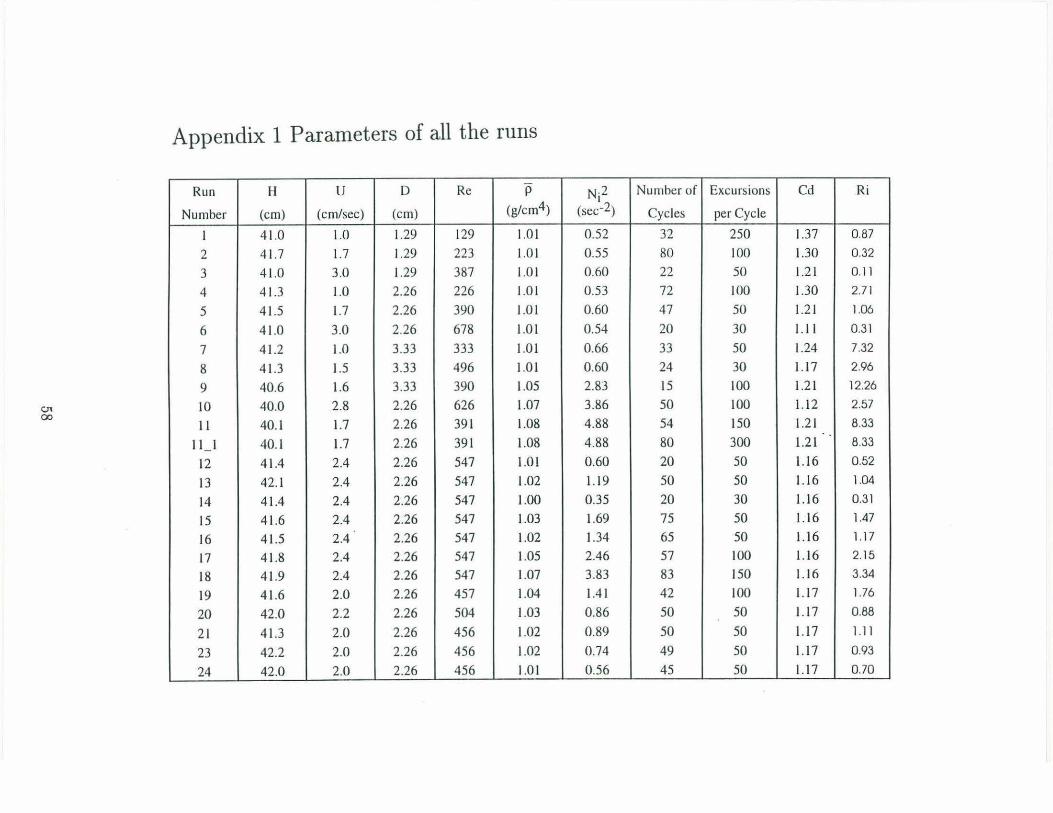
The parameters of all the 75 runs are listed in Appendix 1: and every run is plotted

in the (Re, Rio) space as illustrated in Figure 2-2. Re was varied from around 100

to 1600 and Rio from 0.2 to 12.3. Since keeping Re constant is easier than preparing

the same stratification for each run , the runs are aligned along a cons tant Re line in

the (Re, Rio) phase space.

2.2.3 Data Correction

The conductivity profile was converted to a density profile usmg the reading from

the five samples of water with the density known to 10-4 g/ cm3. The raw density

profile was processed before any calculations were made, although it showed trends

or characteristics clearly. First, density was extrapolated to top 5mm and bot tom 1cm

where the conductivity was not measured. Second, sometimes the probe generated

noise spontaneously. This happened in the later stages of some runs. The data

was smoothed by applying 9 point moving average. Third, the linear drift of the

probe was corrected using mass conservation. The total mass of the fluid should be

conserved during a run , if the effect of evaporation is neglected. The evaporation was

at most less t han 1mm/ day . The evaporation caused less t han 5% changes of the

mean density throughout a run, and all the density profiles of a run were shifted to

give the same mean density. The conductivity probe is very sensitive to temperature

change. During a run , the room temperature changed less than 2°C over a day, and

17

0 >< >< 0

\D

·c: 0 0 >< >< >< >< ><

·;;n 0 "<:t

<U c I-. 0

·;;n <U I-. 0 b.() 0 c: ('.I

'i: <U >---~ -I 0 < c: c 0 0 0

>< >< c 0 § b.() <U <U I-. ..c: b.() .... II c: ><

"i: 0 ~

<U 0 ~ >--- 00 ~ >< <U >< ..c: .... ><

>< ><>< {:i 0 0

00 r- V") "<:t \0 ->< - .- ><><- >< -0 >< >< >< ><

>< >< >< >< >< >< >< >< 0

0 >< V")>< >< * 0

>< "<:t 0

><

"<:t ('.I 0 >< * 0 ('.I

*

0 N 0 ' 0 0 0 0

zn! z! N za = 0 !H

Figure 2-2: The stability curve and all the 75 runs in the (Re, Rio) space. Here, *is for 1.29cm diameter rod, x for 2.26cm rod , and o for 3.33cm rod. In the figure, the hatched region denotes a marginal region. The region above the hatched region is an unstable region (the layering region) and below is a stable region (the non- layering region). The boundary between the marginal region and the layering region is the stability boundary. The numbers in the figure denote runs shown in the following figures .

18

the effect of the temperature variation was neglected. Th e corrected data set was

used in the potential energy calculation.

19

Chapter 3

Observations

3.1 The evolution of the density profile

Every run exhibited the development of mixed layers at the top and bottom of the

tank before significant variations happened to the interior density field. The condi­

tion of zero flux across the horizontal boundaries requires vanishing vertical density

gradient so that boundary mixed layers are produced. These boundary mixed layers

are independent of the layer produced in the interior, which is the focus of this study.

Initially the thicknesses of the boundary mixed layers are less than the turbulent re­

gion, which is the same as the depth of the tank. The boundary mixed layers expand

into the stratified interior with time due to the no flux condition at the horizontal

boundaries . Thus the expansion of the boundary mixed layer does not require an

increase in the turbulent region or an increase in the strength of turbulence. The

structure of the boundary mixed layers is basically the same in every case. The den­

sity gradient was close to zero and varied smoothly. However, the interior showed

different patterns of evolution depending on the external parameters such as Re and

Rio.

For fixed Re, the evolution of the interior density structure is described for different

values of Rio. For small Ri0 , the density profile shows two boundary mixed layers and

the interior of almost constant density gradient. The transition from the boundary

layers to the interior is smooth. No intensification of density gradient is observed as

20

shown in Figure 3-1a. Re and Rio of this run (Run 14) are 547 and 0.31, respectively.

The interior density gradient looks like a wide plateau in each profile with small scale

"wiggles" of about 1.3cm as shown in Figure 3-1b. The wiggles are present from the

beginning to the end of the run. They were observed in many cases regardless of the

external parameters but did not become amplified in any case. They were presumably

due to turbulent fluctuations . Since the wiggle length scale is never amplified in any

runs , the presence of these small wiggles is henceforth neglected when explaining the

st ructure of the interior. As time progresses, the height of the plateau decreases very

slowly. The width also decreases monotonically due to the expansion of the boundary

layers. Figure 3-2 is a series of shadowgraphs taken during Run 14. The black vertical

st rip is the stirring rod of diameter being 2.26cm. No interface can be found.

For a run with larger Ri0 , interfaces form first between the interior and boundary

mixed layers as shown in Figures 3-3a and 3-3b. Re and Rio of this run (Run 13)

are 54 7 and 1.04, respectively. The density gradient shows a clear difference from the

preceding density gradient, which is Figure 3-1b, but the density profile only seems

slightly different when Figures 3-1a and 3-3a are compared. These two interfaces

intensify rapidly at early t ime and then approach each other while keeping their

strength up to a certain distance. At the same time, the mean interior density gradient

decreases slightly, as shown in Figure 3-3b. When the two interfaces become close

enough, one of them becomes weaker and decays. At this point, the fluid becomes

two mixed layers with an interface. The remaining interface also decays and the fluid

becomes homogeneous. During this run, the small scale wiggles are also observable.

The interfaces are about 5cm thick, but t he wiggles are about 1.3cm thick. The

interfaces are thicker than the wiggles so there is no difficulty in telling them apart.

Sometimes, the wiggles override the interfaces. This run shows the formation of

two coherent interfaces, and an interior layer, characterized by a decrease in density

gradient , between t he interfaces. The formation of interfaces is not observed during

the runs with lower Rio such as Run 14. A transition point is expected between the

runs with t hese characteristics and the runs with lower Ri0 •

For a run with even larger Rio, interfaces and layers form in the interior as illus-

21

35

30

25

20

15

10

5

OL---------~~~~~-L~L--L~~_L~~~~

1.0 I 1.02 1.03 1.04 1.05 1.06

p (glcm3)

(a)

E u

E 0 ~

2

- dp/dz (glcm4) xiO-J

(b)

Figure 3-1: The evolution of the density field during Run 14. The values of Re and Rio of this run are 54 7 and 0.31, respectively, and they are below the stability curve in Figure 2-2. (a) The density profile of the initial state and after at every 60 excursions. Each plot is shifted by 0.005g / cm3 . (b) The negative of the gradient of the density profiles in (a). Each plot is shifted by 0.0005g f cm4 •

22

(a) (b)

(c) (d)

Figure 3-2: A series of shadowgraphs taken during Run 14. The screen was placed about lm in front of the tank . Pictures were taken during (a) 5th excursion, (b) lllst excursion , (c) 219th excursion, and (d) 639th excursion. The vertical black strip is the stirring rod with D = 2.26cm. The signature of mixing becomes weaker over t ime. The signature of turbulent mixing is weak near the top and bottom boundaries.

23

40

35

30

~ 25

E u f::

20 :I: 0 Ui :I:

15

10

5

0 1.02 1.04 1.06 1.08 1. 1

p (glcm3)

(a)

40

35

30

25 E u f:: :I: 0 Ui :I:

15

0.002 0.004 0.006 0.008 0.01 0.012

- dp/dz (g/cm4)

(b)

Figure 3-3: The evolution of the density field during Run 13. The values of Re and Rio of this run are 54 7 and 1.04, respectively, and they are slightly above the stability curve in Figure 2-2. (a) The density profile of the initial state and after 150, 300, 450, 750, 950, 1150, and 2250 excursions. Each plot is shifted by 0.01g j cm3

• (b) The negative of the gradient of the density profiles in (a) . Each plot is shifted by 0.0015gj cm4

• The interior mean density gradient slightly decreases over time.

24

trated in Figure 3-4. In this case (Run 18), Re and Rio are 54 7 and 3.34, respectively.

The boundary mixed layers advance rapidly after the beginning of mixing, and then

the expansion rate slows down as the interior structure is well established. After this

time, the boundary layers do not continue to expand. Instead, t he interfaces between

the boundary layers and the interior stay at the same position and become weaker

while intensifying the adjacent interfaces. The interfaces eventually decay so that

the boundary layers show sudden expansion into the interior. The interior density

structure changes over t ime, which is explained in the next section. Figure 3-5 is a

series of shadowgraphs taken during Run 17, whose Rio of is 2.15 and Re is 54 7. The

interfaces, which are white lines, are maintained under active turbulent mixing. In

Figure Sa thin white lines can be seen between the thick white lines. They are the

small scale wiggles of about 1.3cm thick.

One result of the instabili ty theory of Phillips / Posmentier is t he intensification

of the interior density gradient if Rio > Ric. If Rio < Ric, t urbulence should

smooth out perturbations from the mean state so that the formation of a coher­

ent interface or the intensification of density gradient is not possible. Another re­

sult of Phillips / Posmentier 's theory is a decrease of the density gradient between

the interfaces. The evolution of a linear density profile to coherent interfaces while

weakening the density gradient between the interfaces, as shown in Figures 3-3b

and 3-4c, is defined as a layering. The layering is the mos t clear evidence of the

Phillips/ Posmentier 's instability theory. The stability boundary, which is equivalent

to Ric, is found by varying Re and Rio as shown in Figure 2-2.

In Figure 2-2, the hatched region denotes a marginal region , where a transition

from a non-layering to the layering occurs. The layering clearly happens above the

marginal region. Below the marginal region the layering is not observed. In the non­

layering region, transient interfaces are observed, instead of the coherent interfaces.

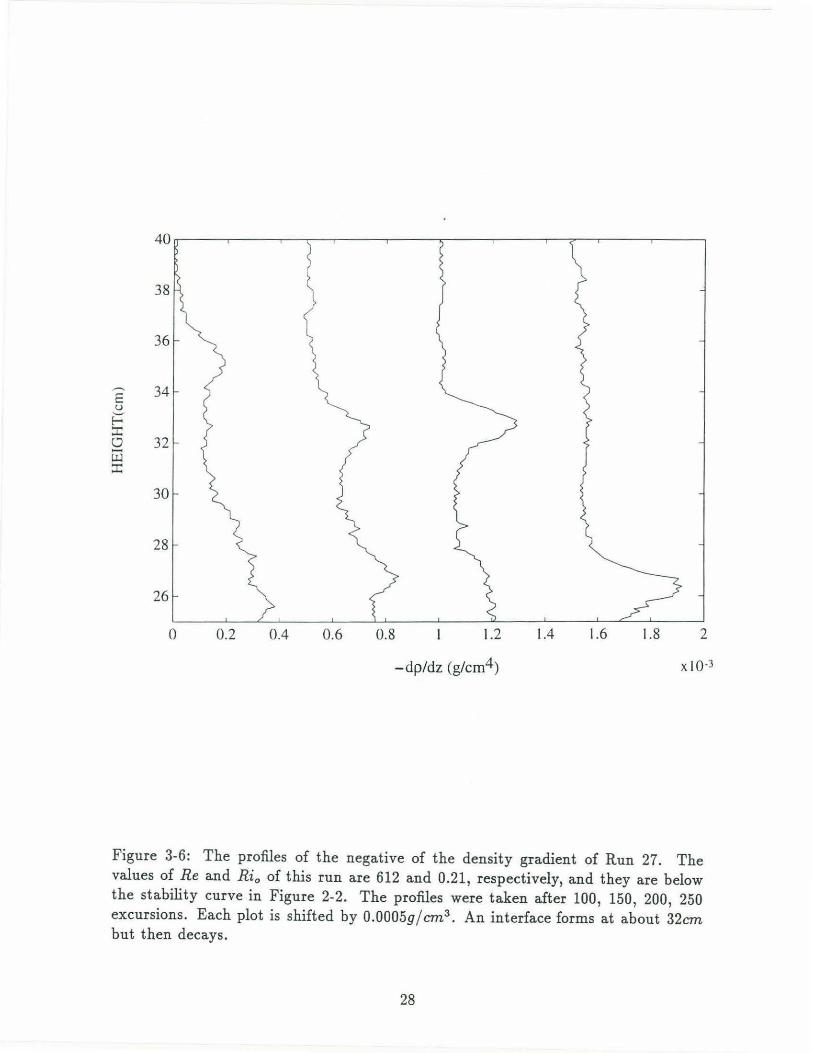
An example of the transient interface is shown in Figure 3-6 (Run 27). Re and Rio

are 612 and 0.21, respectively. An interface forms at about 32cm after 150 excursions

but then decays between 200th and 250th excursion. In the marginal region, the

evolution of the density field is not clear. The upper boundary of the marginal region

25

1.05 1.1 1.15 1.2 1.25 1.3 1.35 1.4

p (glcm3)

(a)

40

35

30

25 E u

f=' 20 ::!:

v u:i - 15

10

5

0 0 0.05 0. 1 0. 15 0.2 0.25

- dp/dz (glcm4)

(b)

Figure 3-4: The evolution of the density field during Run 18. The values of Re and Rio of this run are 547 and 3.34, respectively, and they are far above the stability curve in Figure 2-2. (a) The density profile of the initial state and after 300, 750, 1050, 1500, 1800, 2700, 3000, 3750, and 4500 excursions. Each plot is shifted by 0.01gj cm3 . (b) The negative of the gradient of the density profiles in (a). Each plot is shifted by 0.02g J cm4

• The boxes in the figures are an example of the decay of an interface. During the decay the interface thickness increases.

26

(a) (b)

(c) (d)

Figure 3-5: A series of shadowgraphs taken during Run 17. The values of Re and Rio of this run are 547 and 2.15, respectively, and they are above the stability curve in Figure 2-2. The screen was placed about 1m in front of the tank. Pictures were taken during (a) 402nd excursion, (b) 582nd excursion, (c) 678th excursion, and (d) 800th excursion. The vertical black strip is the stirring rod with D = 2.26cm. The two white strips near the bottom boundary come close over time become one. This is a visual example of the merging of interfaces .

27

40

38

36

...---. 34 E u .._.. f-::r: 0 32 -UJ ::r:

30

28

26

0 0.2 0.4 0.6 0.8 1.2 1.4 1.6 1.8 2

-dp/dz (g/cm4) X J0-3

Figure 3-6: The profiles of the negative of the density gradient of Run 27. The values of Re and Rio of this run are 612 and 0.21, respectively, and they are below the stability curve in Figure 2-2. The profiles were taken after 100, 150, 200, 250 excursions. Each plot is shifted by 0.0005gj cm3 • An interface forms at about 32cm but then decays.

28

is defined as a stability boundary, which is Ric. The relation between Ric and Re is

l R. Re og 'I. e ~ 900 '

for 400 < R e < 1000. ,..., ""

According to t he theory of P osmentier (1977), if Rio is slightly larger t han Ric, the

difference between the layer and interfacial density gradients is small. The mixing

efficiency, R 1, is high near Ric so that the boundary mixed layers might expand

rapidly and overtake the interior before interior layering becomes st rong enough to be

observed. Thus, the present experiments might overestimate the stability boundary.

The overall Richardson number of the stability boundary increases as the Reynolds

number increases. For fixed Re, there is a critical Richardson number Ric. Thus, in

the (Re, Rio) parameter space, layering happens when Rio increases from zero along

constant R e line, and this behavior is consistent with t he results . Although, t he

present experiments cannot find Ric precisely, they show the t rend clearly. For high

Re, due to the rapid advance of boundary mixed layers and high R,, the marginal

region expands as illustrated in Figure 2-2. For high Re, due to t he saturation of salt,

it was not possible to get Rio > Ric. Thus, increasing Re beyond about 1000 while

maintaining the experimental set up is not useful.

3.2 The evolution of the interior layer

For the runs with Rio > Ric, an initially uniform stratification turns into a senes

of small steps, which become larger and stronger over time. Figures 3-7a and 3-

7b, are sequences of t he profiles of the density and density gradient taken during

Run 4, whose Re and Rio are 226 and 2.71 , respectively. The steps are in t he form

of periodic perturbations to the mean density gradient. Naturally, the height of

the peaks in density gradient increases by decreasing the density gradient of layers.

Figure 3-7 clearly shows the intensification of the interior steps. The sizes of steps

increase through a merging or decay of interfaces, which is discussed in the next

29

E u

f::' :I: 0 Ui :I:

E' u f::' :I: 0 Ui :I:

1.01 1.02

0.005

1.03 1.04 1.07

(a)

0.01 0.015

-dp/dz (glcm4)

(b)

Figure 3-7: The evolution of the density field during Run 4. The values of Re and Rio of this run are 226 and 2. 71 , respectively, and they are above the stability curve in Figure 2-2. (a) The density profile of the initial state and after every 300 excursions. Each plot is shifted by 0.0005g / cm3 . (b) The negative of the gradient of the density profiles in (a). Each plot is shifted by 0.002g/ cm4 • The boxes in the figures are an example of the merging of interfaces.

30

section, as shown in the figure. Eventually the density profile becomes a senes of

well-mixed layers with sharp density interfaces. The interior structure seems to reach

a steady state or an equilibrium state after some t ime. After this time, the merging

or decay of interfaces usually happens due to the advance of boundary mixed layers,

and the interior almost does not show any evolution. The boundary layers eventually

overtake the interior so that the fluid becomes homogeneous.

3.3 The merging and the decay of interfaces

After the initiation of the layering, small layers and interfaces merge and the steps

become larger. The decay of interfaces was observed and explained by RMT. When

the density differences across two adjacent interfaces are different, the density flux

across the weak interface is larger according to the theory of Phillips / Posmentier.

As a result, divergence occurs at the weak interface, causing eventual decay, while

intensifying the adjacent interface. An example of the decay is in Figure 3-8a, which

is a sequence of the density gradient profiles of Run 2. The Re and Rio of this run

are 223 and 0.32, respectively. During the decay both the thickness and positions of

t he interfaces do not change. The weaker interface just decays. In the interior, the

decay is very rare.

The expansion of the boundary layer usually causes the decay of an interface, and

the small boxes in the Figures 3-4a and 3-4b are an example. During the decay caused

by the expansion of the boundary mixed layers, the interface thickness increases . The

decay of interface is also observed at the ends of some runs. For runs with Rio > RiC)

the fluid eventually turns into two mixed layers. As time progresses, the density jump

across the interface, 1:1p, decreases slowly while the thickness of the interface remains

almost constant as shown in Figure 3-8b, which is a sequence of density profiles taken

during Run 18 after the fluid becomes two mixed layers.

The merging of interfaces occurs when two interfaces are close, i.e., a layer is t hin.

The merging happens even when the density differences across two adjacent interfaces

are similar so that a divergence of density flux cannot happen. This implies that there

31

28

26

24

e ~ 22 :I: 0 Ui 20 :I:

18

16

14

25

24

23

e 22 u !=" :I: 2 1 0 Ui :I: 20

19

18

17

0.0 1 0.0 15

- dpl dz (g/cm4)

(a )

16~--------~--~~--~--~--~--~~---L--~ 0 0.05 0. 1 0. 15 0.2

- dp/dz (g/cm4)

(b)

Figure 3-8: The examples of the decay of interface. (a) The decay of an interior interface during Run 2. The values of Re and Rio of this run are 223 and 0.32, respectively, and they are above the stability curve in Figure 3. The negative density gradient profiles of the initial state, after 1000, and then every 200 excursions. Each plot is shifted by 0.002gj cm4 • (b) The decay of an interior interface during Run 18. The negative density gradient profiles of the initial state, after 3000, and then every 750 excursions. Each plot is shifted by 0.018g / cm4

• The thickness of the interface stays the same until almost the end of the run while the density difference across the interface gradually decreases.

32

is a minimum length scale of a layer, but the present experiments cannot verify clearly.

In the interior, the merging occurs during the early stage of a run. Through merging

a new interface forms from the two previous interfaces so the length scale of layer

gets larger. The data shows that when the merging occurs, the interface gets thicker

and the new interface shows a larger density .difference across it . The small boxes

in Figures 3-7a and 3-7b are good examples of the merging. The expansion of the

boundary mixed layers also cause the merging and Figure 3-5 is a good visual example

of the merging. The two white stripes near the bottom of the tank come close and

eventually become one.

The merging and decay seem to stop and the interior reaches an equilibrium

state. After this state, the decay is usually observed along with the expansion of

the boundary layers and the decay of the interior interface is rarely observed. The

merging of the interior interfaces is not observed during the equilibrium state.

33

Chapter 4

Analysis

4.1 The length scale of layers and interfaces

Although the theory of Phillips/ Posmentier does not predict any length scale of the

steps, the density profiles such as Figure 3-7 shows the existence of one. To find what

factors might determine the length scale of steps, the sizes of the steps are compared

with the external length scales of the experiments, which are the diameter of the

rod , D, and U / Ni. Here, U is the speed of the stirring rod and Ni is the buoyancy

frequency of an initial stratification.

Measuring the thicknesses of an interface and an interior mixed layer , separately,

1s rather ambiguous, since there is no clear border between an interior mixed layer

and an interface. But the combined thickness of a layer and an interface can be

measured clearly with the plot of vertical density gradient such as Figures 3-3b and

3-4b. The vertical density gradient is a sharp peak at an interface and constant or

minimum value in an interior mixed layer. The distance between two adjacent peaks

is defined as a step size, l$, when two peaks are of similar sizes. When there are only

two interfaces , they approach each other with time due to the expansion of boundary

mixed layers. In such cases, the minimum distance that the adjacent peaks achieve

before they vanish was considered as a step size as long as the interfaces are the same

strength. As explained in section 3.2, the length scale changes with time due to the

merging and the advance of the boundary layers. The spacing between the interior

34

peaks also shows spatial variation. Thus, the minimum distance between two peaks

of same strength that do not merge is taken as the step size. In Table 1, the results

are listed with the external parameters. The relation between the step size, l 3 , and

U I N; is plot ted in Figure 4-1.

The size of the step is compared with the .external length scales . There are two

pairs of runs that have similar parameters except t he sizes of rods . One pair is Runs 2

and 5, and the other is Runs 4 and 7. The size of rod, D, is increased 75% and 47%,

respectively, but the sizes of step do not change significantly as can be seen in Table

1. As shown in Figure 4-1, the run with D = 1.29cm generate larger step, but the

runs with D = 3.33cm generate smaller steps. Runs with D = 2.26cm show large

changes in step sizes. It is clear that the sizes of rods do not determine step sizes. On

the other hand, 13 and U I N; show a tendency for a linear relation. The correlation

coefficient between 13 and U I N; is 0.85. In the figure, the solid line is a least square

fit to the data. The formula for the line is

u 13 = 2.6- + l.Ocm.

N;

As Rio decreases to the stability boundary by decreasing U IN;, 13 increases. If

the above relation continues to hold down to the stability boundary, 13 becomes

comparable to the depth of the tank near the stability boundary. Thus, the depth

of the tank becomes a strong obstacle in observing layering. An experiment with a

deeper tank is necessary to extend the investigation of the dependence of l 3 upon

U IN; down to t he stability boundary.

4.2 The spectrum of the density gradient

With the density gradient profile , a spectral analysis was done to see the change of

the length scale more clearly. Each profile was divided in to 256 subintervals and a

Hanning window was applied to each subinterval. Actual calculation was done with

Matlab built in function called spectrum. Since the data set is finite, the resolution

35

Run Step Size u N· U/N· D 1 1

Number (em) (em/sec) (sec-1) (em) (em) 2 6.6 1.70 0.74 2.29 1.29 4 3.2 1.00 0.73 1.37 2.26 5 6.9 1.70 0.77 2.19 2.26 7 3.2 1.00 0.81 1.23 3.33 9 3.4 1.60 1.68 0.95 3.33 10 3.7 2.77 1.96 1.41 2.26 11 4.0 1.73 2.21 0.78 2.26 15 6.2 2.42 1.30 1.86 2.26 16 7.6 2.42 1.16 2.09 2.26 17 5.5 2.42 1.57 1.54 2.26 18 5.3 2.42 1.96 1.24 2.26 19 4.7 2.02 1.19 1.70 2.26 21 7. 1 2.02 0.94 2. 14 2.26 22 6.5 2.02 1.06 1.91 2.26 23 6.6 2.02 0.86 2.35 2.26 26 8.8 1.67 0.56 3.00 2.26 28 5.3 1.26 0.54 2.34 2.26 54 5.8 3.24 1.98 1.63 2.26 79 8.7 2.42 1.03 2.34 2.26

Table 4.1: The sizes of steps and the external length scales, D, and U/ Ni

36

10

9 X

8 X

7 X X

,.--.. *X E X

u X .......- 6 0.. X ~ X (/) X X '+- 5 0

X v N

(/) 4 X v X ..c E- 0

o: D = 3.33cm 3 0 X

x: D = 2.26cm

2 * : D = 1.29cm

OL-------~------~------~------~------~------~------~ 0 0.5 1.5 2 2.5 3 3.5

U/Ni (em)

Figure 4-1: The relation between the sizes of the steps and the external parameters, D and U / Ni . The data for this figure is in Table 1. The solid line is the least square fit to the data points. Here, * is for 1.29cm diameter rod, x for 2.26cm rod , and o for 3.33cm rod.

37

becomes coarse as the length scale increases.

Almost all spectra showed a peak of length scale 1.3cm but this does not grow

and stays independent of other peaks as shown in Figure 4-2. These small peaks were

presumably due to turbulent fluctuations. The presence of these peaks is neglected

during the explanation of the spectrum. The spectrum also shows the difference

between the layering case and non-layering case. The layering case shows persistent

peaks but the non-layering case shows temporally varying peaks as can be seen in

Figure 4-2. The initial state is a smooth spectrum in both cases but layering case

showed growth of some peaks with time as can be seen in Figure 4-3. The initial peak

occurs at relatively short scale and a peak of longer scale occurs later. The short scale

peak becomes weaker and eventually the peak of long scale dominates . This state

is maintained until the boundary mixed layers overtake the interior. During the

second and third cycle of Run 15, spectrum shows a peak at 3.8cm as can be seen

in Figures 4-3b and 4-3c. During the third cycle, the peak moved to a longer scale,

6.6cm, as shown in Figure 4-3d. In the figure , the dotted line is the spectrum of sixth

cycle. It clearly shows the intensification of the peak at 6.6cm.

Though the spectrum shows the increase of the step size clearly and consistently

with the analysis of Section 4.1, due to the finite size ofthe data set, this quantification

of the length scale is not as useful as the measuring of t he spacing between peaks in

density gradient, as was done in Section 4.1.

4.3 Energetics

The speed of the stirring rod was known accurately so that the work done to the test

fluids was estimated using drag coefficient with the equation

Work Done 1_ 2

one Excursion = 2/ Cd U L H D.

Here, H is the depth of the tank, L the length of an excursion, p the mean density of

the fluid, U the speed of the rod, D the diameter of the rod, and Cd drag coefficient. Cd

38

I I

0 0 ,....... -,........_ ,........_ .D '"0 '-/ '-/

~ N I

0 0 ,....... ,.......

(") (") I I

0 Mo 0 Mo "!" r-;- -,....... "!" r-;- -,.......

I I I I

0 0 0 0 0 0 0 0 ,....... ,....... ,....... ,....... ,....... ,....... ,.......

,......_

I

0 E

0 0 E 0 .._, ,.......

11) ,.......

ca u

Cl)

..s:: On c:

E 11) -I ....J I

~~ 0 0 ,....... ,.......

,........_ ,........_ ro u '-/ '-/

~ N I

0 0 ,....... ,.......

C( C(

0 Mo vo "!" r- -- "( 00 - -,.......

I I I I I I

0 0 0 0 0 0 0 0 ,...... ,....... - ,....... ,....... ,.......

Al!suga !Bll::>gds JgM.od

Figure 4-2: The density gradient spectrum of Run 14, one of the non-layering cases. (a) The initial state, after (b) 60, (c) 120, and (d) 180 excursions.

39

~~~--~no.-r-~rn,-r-~ ~ .......

0 0

0 E 0 - u \0

E ,-..., \C) ,-..., u ..0 "'0 OC?---7 '-...-/ '-...-/ M

~ N 0

0 0 - -"'( ("")

0

No No \0 a:' --"'( '9 a:' -- "'(

0 0 0

0 0 0 0 0 0 0 0 - - - - -""""'

I

E 0 E 0 0 0 - d) -~

u U)

..c eo c:

E d)

0 .....l 0 u 0 0 C"!---7

,-..., ,-..., C\j u

'-...-/ '-...-/

N ~ 0

0 0

"'( ~~~L-~UL~~~~~-L~N 0

<"( '9 ~ ""7 ~ 0 0 0 0 -

"'( No

"'( '9 "' - ....... 0 0

0 0 0 0 - - - -Figure 4-3: The density gradient spectrum of Run 15, one of the layering cases. The values of Re and Rio of this run are 54 7 and 1.4 7, respectively. (a) The initial state, after (b) 50, (c) 100, and (d) 150 and 300 (the dotted curve) excursions.

40

was obtained from Figure 5.11.6 in Batchelor (1969). The total work done generated

both internal waves of amplitude 1cm and turbulence. How much of the work done

to the fluid was used to generate the internal waves is not clear. But, a few number

of excursions was enough to supply energy for the internal waves. The rod moved

perpendicular to the density surfaces and the rod was not a good wave maker. Also,

the wave energy cannot radiate out of the tank, so the energy used to generate internal

should be far less than that used to make t he turbulence.

The total work done must be dissipated in two ways, by friction and by increasing

the potential energy of the fluid by mixing the stratification. With the density known

at millimeter interval, the change of potential energy of the fluid , tlP.E. , is calculated

using the definition

1top

tlP.E.(t ) =A (Pi(z) - p(z ))g z dz. bottom

Here, A is the area of the tank, Pi( z) the initial density profile, and p( z ) a density

profile measured at later time. The vertical integration was done using the modi­

fied Simpson's Rule. The work done and tlP.E. are normalized with the difference

of potential energy between the initial state and the completely mixed state. The

normalization constant of each run is listed in Appendix 2.

With the estimated work done and tlP.E. a mixing efficiency, or the flux Richard­

son number R,, is defined as

the change of the potential energy for a certain time interval Rt= ------~----~~--------~~-------------------

work done to the fluid for that time interval

As explained before, the work done to the fluid generated some internal waves, which

were observed with a shadowgraph, and expected to be dissipated as heat. Because

of these internal waves, this definition would underestimate R1 in an oceanic envi-

ronment.

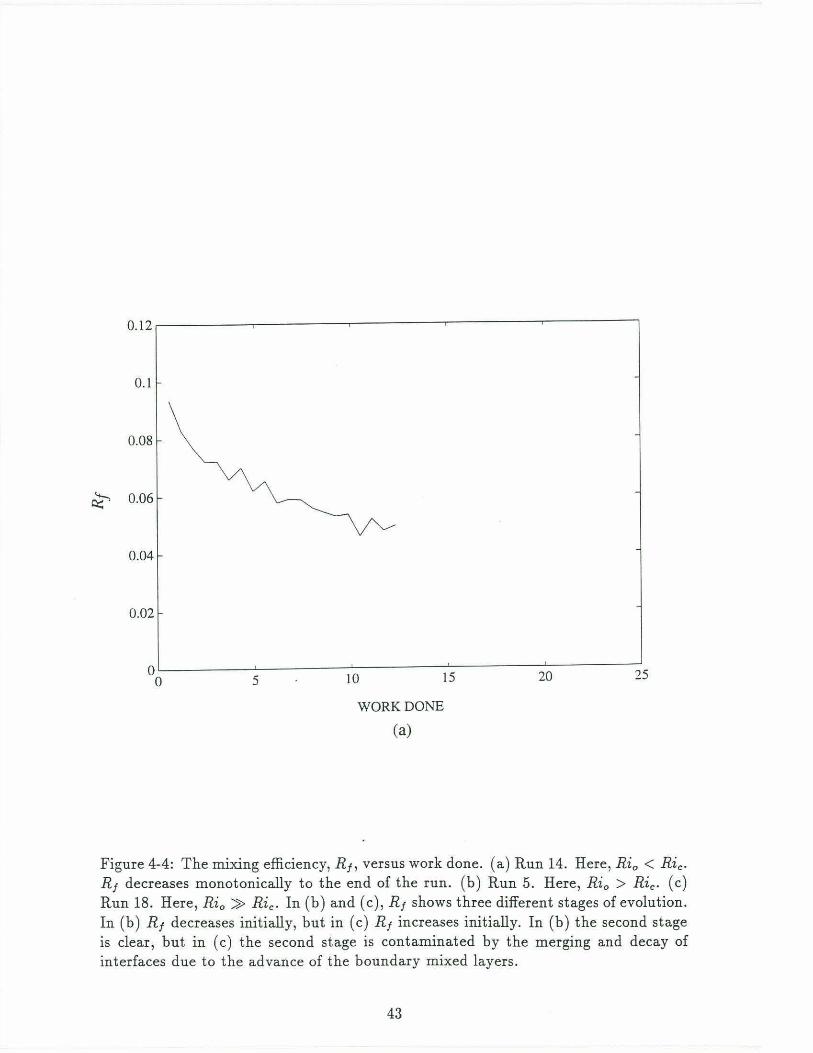
In the non-layering case, R1 monotonically decreases over time as shown in Fig-

41

ure 4-4a, which is observed in Run 14. The decrease is probably explained by the

expansion of the boundary mixed layers. In these boundary layers, there is little

stratification to mix, so the work done to the boundary layers is far more than the

potential energy stored in the stratification, and the most of the turbulent kinetic

energy is dissipated as heat. As the boundary layers expand an increasing amount

of work done on the fluid is dissipated as heat so that Rt decreases along with the

expansion of the boundary mixed layers. Figures 3-2b, 3-2c, and 3-2d, which are

shadowgraphs taken during Run 14 (a run with Rio < Ric ) show the signature of ac­

tive turbulence mixing in the interior, but the signature of mixing is greatly reduced

in boundary mixed layers.

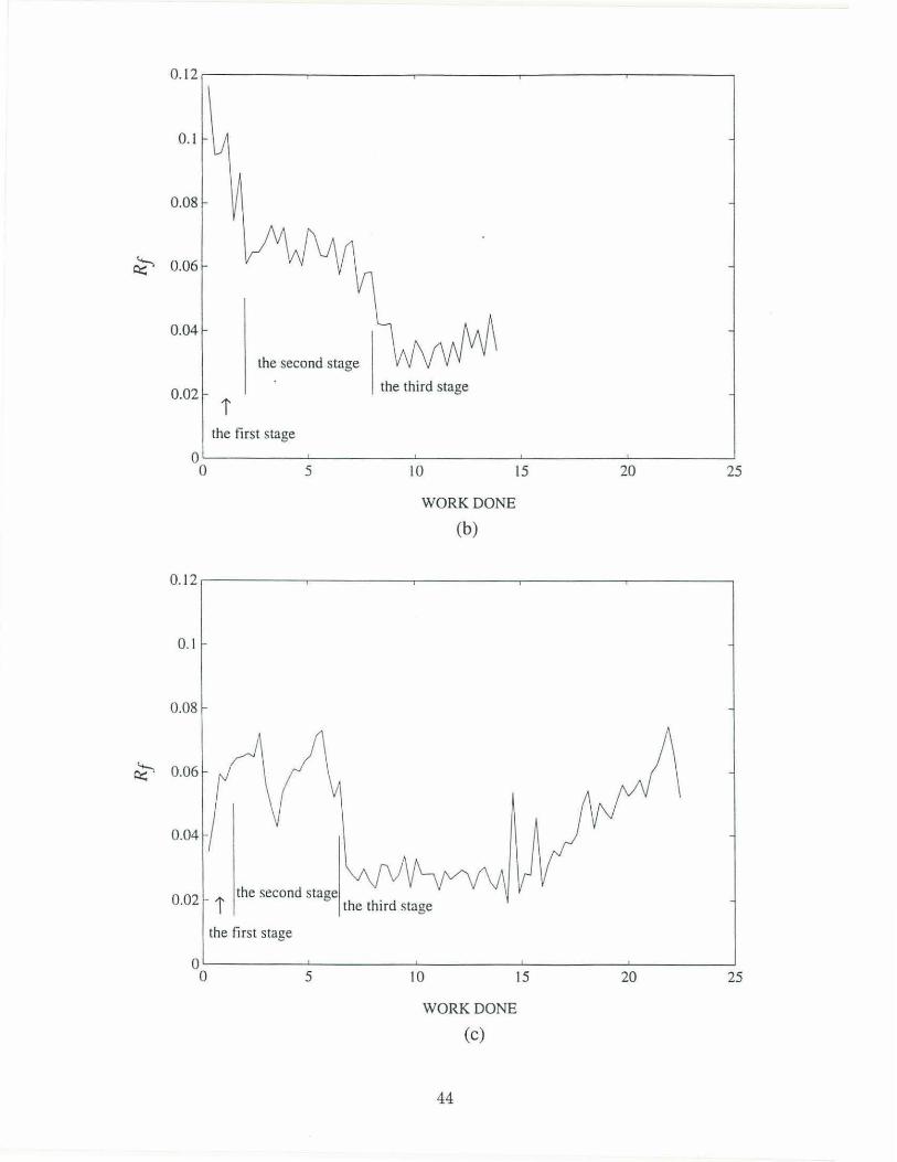
In the layering case, R1 can be divided into three stages of evolution related to

the different stages of the density field evolution; 1. the initiation of steps, 2. the

equilibrium state, and 3. two layer state. The first stage shows two completely

different patterns of R1 evolution. For Rio ~ Ric, there is a decrease of Rt during the

first stage as in the non-layering case. But the decrease yields to the second stage,

where R1 is rather constant as shown in Figure 4-4b. However, another pattern is

seen for Rio » Ric, i.e., for Rio far away from the stability boundary. In this case Rt

sharply increases during the first stage as shown in Figure 4-4c. In Figure 4-5a, for

fixed Re, the early changes of Rt are plotted for the different values of Rio. As Rio

increases , the decrease of R1 during the early stage changes to an increase but when

the transition occurs is not clear. In Figure 4-5b, the early changes of Rt during the

runs with high Rio are shown. All of them clearly show the initial increase of R,.

According to Posmentier (1977), R1 of the equilibrium state should be less than

that of the initial state. However, the change of Rt during the development of the

steps does not have to be monotonic. Here, it is not clear whether the decrease

verifies the prediction of the theory, or the decrease is due to the expansion of the

boundary mixed layers. The initial increase seems to contradict Posmentier's the­

ory. Turner (1973) discussed the energetics of layering in the presence of turbulence.

Initially, stratification is so large that turbulence cannot mix the stratification ef­

fectively. By developing a step-like density structure, the local gradient Richardson

42

0.12 r-------r-----.------.------,.------,

0.1

0.08

~ 0.06

0.04

0.02

00L_ ________ 5~------~10--------~15~------~2~0--------~25

WORK DONE

(a)

Figure 4-4: The mixing efficiency, Rf, versus work done. (a) Run 14. Here, Rio< Ric. Rt decreases monotonically to the end of the run. (b) Run 5. Here, Rio > Ric. (c) Run 18. Here, Rio~ Ric. In (b) and (c), Rt shows three different stages of evolution. In (b) R1 decreases initially, but in (c) Rt increases initially. In (b) the second stage is clear, but in (c) the second stage is contaminated by the merging and decay of interfaces due to the advance of the boundary mixed layers.

43

0. 1 2.---------,---------~----------~---------.---------.

0.1

0.08

~ 0.06

0.04

the second stage

the thi rd stage 0.02 i

the fi rst stage

0~--------~--------~----------~--------~--------~ 0 5 10

WORK DONE

(b)

15 20 25

0. 12 ,-----.-------,------ -,-------.,..--------,

0.1

0.08

~ 0.06

i the second stage

0.02 the thi rd stage

the fi rst stage

0~--------~--------~----------~--------~--------~ 0 5 10

WORK DONE

(c)

44

15 20 25

0.12

0.1

0 0

0 0

0 0 • p . 0 0 • 0 ' o

0 0 '0 0.08 0 0 0 . 0 • + 0 0

0 + + 0 • X + • + + + + •

+ X + + +

+ X

~ 0.06 X • +

+

0.04 ..

0.02

0 0 0.5 1.5 2 2.5 3 3.5 4 4.5 5

WORK DONE

(a)

0.12

0

0 0 0

0.1 0 0 0

0 0

0.08 0 + X

+ + + X +

~ 0.06 • + + + + • • + +

+

+ +

0.04

0.02

0 0 0.5 1.5 2 2.5 3 3.5 4 4.5 5

WORK DONE

(b)

Figure 4-5: Examples of the initial change of R1. (a) Re is fixed at 547. Rio is x:3.3 (Run 18), +:2.2 (Run 17), o:l.5 (Run 15) , *:1.2 (Run 16), and a:0.3 (Run 14). For Rio > Ric, Rf shows a decrease. However, for Rio ~ Ric, R, shows a sharp initial increase. (b) For Rio ~ Ric. All of them show the initial increase. The values of Re and Rio of each case are +:547, 3.3 (Run 18), x:547, 2.2 (Run 17), *:730, 1.9 (Run 54), and o:860, 1.4 (Run 58), respectively.

45

number is reduced locally to a value at which turbulent mixing can be maintained.

One consequence of this discussion is that during the formation of steps more mixing

is allowed in the layers so that the mixing efficiency increases, which is observed with

the runs of Rio » Ric.

A characteristic of the second stage is a nearly constant Rt . In Figure 4-4b, the

second stage is clear but some runs do not have a long enough time for this stage to be

evident. Also the expansion of the boundary mixed layers cause a merging or decay

of interfaces, and contaminates the characteristics as shown in Figure 4-4c. During

this stage, the interior density structure is nearly unchanged.

The border between the second and third stages is clear. Rt sharply decreases.

The advance of the boundary mixed layers result in two mixed layers with a strong

interface between them. A sharp decrease of R1 is observed between the border of the

second and third stages. This phenomenon indirectly supports the relation that R1

decreases as Rio increases beyond Ric· During the t hird stage Rt is nearly constant

as shown in Figure 4-3c, and the experiments become equivalent to the turbulent

entrainment experiments such as Turner (1968) and Linden (1980). Eventually, the

remaining interface also decays, resulting in an increase of Rf, which is discussed in

the next section, as shown in Figure 4-4c.

As explained before, the relation between R1 and Ri is the most important as­

sumption of the stability theory. With the third stage of Runs 17 and 18, i.e. , after the

fluid became two well-mixed layers , the relation between Rt and the local Richardson

number Ri1 is found. The definition of Ri1 is

Ri = g.6.pl I -u?, p -

where, l is the length scale of turbulence, and .6.p the density difference across the

interface. The length scale of turbulence was not measured so that the determination

of l as defined above is not possible. Instead the thickness of the interface is used

for l. The results are shown in Figure 4-5. R1 decreases clearly as Ri1 increases, and

Rt becomes nearly constant for Ri1 2 10. The present experiment was not designed

46

0.1

0.09

0.08

0.07

0.06

• • 0 0 0

~ • • 8 •o

0 0.05 • *

• 0 00

0 0

0.04 0 0 0 0

00 0

0 0

0.03 0 0 o{J ofbo Ill o 0 0

0 0 0 0 0 s 0 0 0

0.02 0 0

0.01

0 0 2 4 6 8 10 12 14 16

Riz

Figure 4-6: Ri1 versus R,. The data during the third stage of Runs 17 and 18 are used. Rf decreases as Ri1 increases and becomes nearly constant for Rit > 10. Here , * denotes Run 17, and o Run 18.

47

to find the relation between R1 and Ri1 so that the increase of Rt from zero as Ri1

increases from zero cannot be found. As Ri1 approaches to zero by decreasing tlp, Rt

should become zero and the increase of R1 as Ri1 increases from zero can be inferred.

Some runs show a decrease of R1 during the decay of the final interface and this

implies the decrease of R1 as Ri1 approaches to zero.

Both the non-layering cases and layering cases near the stability boundary show

a rapid decrease of mixing efficiency during the early stage of the runs. The decrease

is presumably due to the expansion of the boundary mixed layers, in part. Unfor­

tunately, the density profile was not measured often enough to show the very early

change of R f.

4.4 Density flux

Vertical density flux was calculated using mass conservation. The horizontal average

of the mass conservation equation is

8 8 8

tp(z, t) = -8

z F(z, t).

Here, the overbar denotes horizontal averagmg, and F(z, t) is the vertical density

flux. Since the density flux is zero at the horizontal boundaries, vertical integration

of the above equation gives

F(z,t) = 1top 8P~~,t) dz'.

Since the density profile was measured after active turbulence decayed, the measured

density profile was a horizontal average. Integration was done from the top of the tank.

The difference between the two density profiles of before and after a certain cycle was

used for the time differentiation. The calculation satisfies the no flux condition at the

other boundary within a very small error. This shows that both the calculation and

48

probe drift correction were very accurate. In addition, t he density flux calculation

does not contain any ambiguous estimation such as the work done estimation.

The vertical integral of the density flux t imes g, the gravitational acceleration,

gives the time differentiation of potential energy change. The density flux calculated

in t his way has been found to be consistent :with the mixing efficiency analysis in

section 4.3. In non-layering case, the interior density structure changes very slowly

as explained in section 3.1 so that a uniform density flux is expected in the interior.

The density flux contours of a non-layering case are shown in Figure 4-7. The figure

does show a region, which shrinks over time, of nearly uniform density flux . At the

horizontal boundaries, the density flux should become zero, and in the boundary

mixed layers t he density gradient is almost zero. Thus the profile of the density flux

shows a shape of a plateau. As t he boundary mixed layers expand, the width of

plateau decreases while its height stays nearly the same. This causes t he monotonic

decrease of R f as shown in Figure 4-4a.

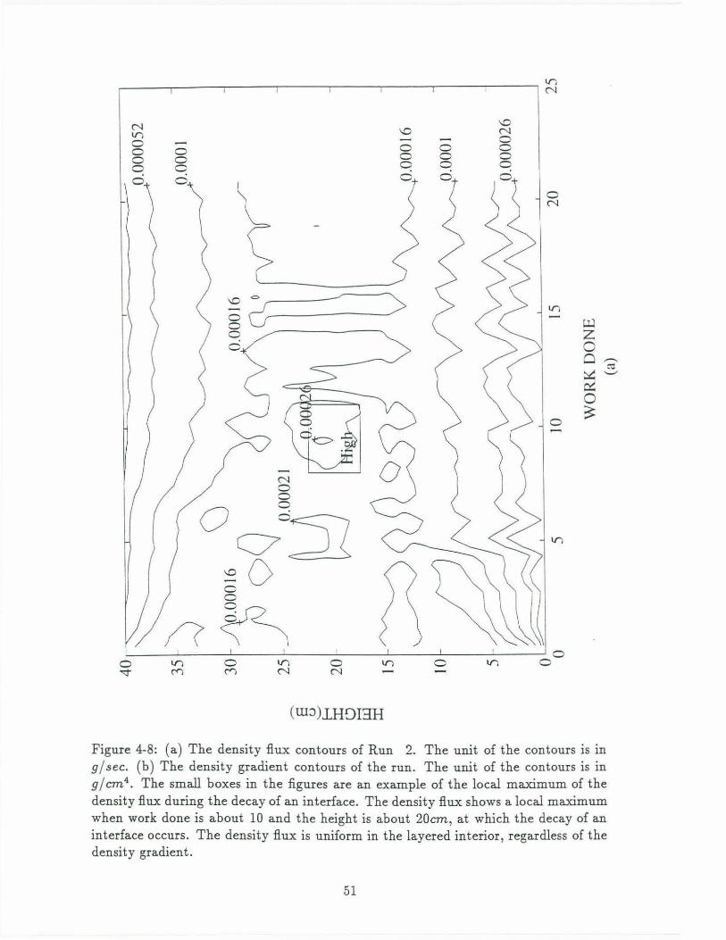
The most prominent feature of the layering case is that the density flux is uni­

form in the layered interior as shown in Figure 4-8a, though the density gradient

varies greatly in the interior as shown in Figure 4-8b. This supports the theory of

Posmentier( 1977) most clearly, since t he density flux should be constant regardless

of the density gradient. The divergence of the density flux is quite small as long as

the interior structure stays the same. At the bottom boundary mixed layer a density

flux is generated, and the flux goes through the interior all the way from the bottom

to the top without changing the interior density structure. It shows that turbulence

can transport scalar properties such as heat, salt, or density further than the length

scale of t urbulent eddies without changing t he structure of t he stratification.

The merging of interfaces results in a local maximum of density flux in time

and space. The small boxes in Figures 4-8a and 4-8b are an example. When the

merging happens t he thickness of the interfaces increases as explained in section 3.3.

Linden( 1979) showed t hat an increase of an interface thickness causes a local increase

of a density flux . As an interface becomes t hicker, the density gradient of t he interface

decreases so that turbulent mixing becomes more effective if the Ri1 of the interface

49

\0 0\ ("t')

0 0 0 0 0 0 0 0 0 0 0 0

(rn~ ).LHDEIH

0 C"l

V')

0

~ z 0 0 ~ 0::: 0 ~

Figure 4-7: The density flux contours of Run 14. The unit of the contours is in g / sec. In the interior the density flux is approximately uniform. The interior density gradient is also uniform as shown in Figure 3-lb.

50

V")

~

~ \0 V) -0 0 0 0 0 0 0 0 0 0

0 0 0 ~

(wJ)lHDEIH

Figure 4-8: (a) The density flux contours of Run 2. The unit of the contours is in 9 I sec. (b) The density gradient contours of the run. The unit of the contours is in 9 I cm4

• The small boxes in the figures are an example of the local maximum of the density flux during the decay of an interface. The density flux shows a local maximum when work done is about 10 and the height is about 20cm, at which the decay of an interface occurs. The density flux is uniform in the layered interior, regardless of the density gradient.

51

t.r) ..........

r.I.l z 0 Q ,-...

~ .0 ....._,

~ 0

0 ~

(w~).LHDEIH

52

is larger than Ric. Secondly, the density difference across the interface disperses

vertically so that more of the turbulent kinetic energy is used to mix the density

difference. Thus, the mixing efficiency increases. The increase of the density flux, F,

also can be explained using the relation between R1 and Ri. During the merging, Ri

of interfaces decreases so that R1 increases. At the layer between the interfaces Ri

locally increase, which causes a local increase of R 1. After the merging a stronger

interface is formed as explained in section 3.3, and Ri of the new interface increases

beyond those of interfaces before the merging and R1 decreases locally. Thus the

merging shows a local maximum in the density flux.

The decay of an interface also shows a local maximum. The density gradient of

an interface decreases during the decay and Ri, too. Turbulence can mix the density

field more efficiently since Ri of the interface is larger than Ric, and t he density flux

increases locally. During the decay of an interface, somewhere within the interface

there should be a point where oplot = -oF(z, t)loz = 0. This means a spatial

extremum of F. Since the magnitude of the gradient decreases

!..__ op = - a2 F > o, ot oz oz2

so the extremum is a maximum.

With the strongest interface formed during the present experiments, the molecular

diffusive flux and the turbulent flux are compared. The molecular diffusive flux Fd =

"'• !:::.p i d. Here "'• is the molecular diffusivity of a salt, !:::.p is the density difference

across the interface, and dis the thickness of the interface. In t he present experiments

the maximum value of !:::.pis 0.066glcm 3 , Dis 2cm, and "'• is 1.5 x 10-5cm2l sec. So,

Fd is about 1 x 10-4 g I sec. The turbulent density flux is more than 1 x 10-3 g I sec,

which is 10 times larger than the molecular diffusive flux. Even at the strongest

interface the turbulent flux dominates.

53

Chapter 5

Conclusions

A linearly stratified fluid was mixed with a rod moving horizontally at a constant

speed. The initially uniform density profile evolves into steps when the overall

Richardson number, Rio, is large and the Reynolds number of the rod, Re, is small.

By changing Re and Rio the stability boundary of layer formation was found. The

stability boundary is consistent with the relation between the mixing efficiency, R,, and Ri0 • The higher Re is, the higher Rio is required to see the layering. The relation

between the stability boundary, Ric, and Re is

. Re log Rtc ~ goo,

for 400 < Re < 1000.

The steps evolve over time. Small steps form first, and they become larger through

the merging and decay of interfaces. The merging occurs between two closely spaced

interfaces. This implies that there might be a minimum step size but the present

experiments cannot verify the idea. The interior seems to reach an equilibrium state.

The merging or decay of interfaces usually occurs due to the advance of boundary

mixed layers after the interior reaches the equilibrium state. Thus, the interior struc­

ture seems to be unchanged after some time, if there is no expansion of the boundary

mixed layers. The size of the equilibrium steps, l~, is a linear function of the external

54

length scale U / Ni, and the relation is

u l~ = 2.6 Ni + 1.0 em.

The analysis of the energetics shows that for Rio > Ric, the change of Rt is closely

related to the formation and decay of steps. While the non-layering case shows a

monotonic decrease of R1 throughout a run, the layering case shows three different

stages. During the initiation of steps, depending on Rio, Rt shows two completely

different patterns of time change. For Rio ~ Ric, Rt decreases initially. Posmentier

(1977) shows that R1 of fully developed steps is smaller than that of the initial state.

The expansion of the boundary mixed layers always decreases Rt and the present

experiments cannot verify the decrease of R1 , which Posmentier predicted, after layer

formation. An experiment with a constant boundary flux is necessary to verify the

decrease.

For Rio » Ric, Rt sharply increases initially, however. The increase is contradic­

tory to the theory of Phillips/ Posmentier. Turner (1973) argues that if stratification

is too strong to maintain turbulence, then by developing a step-like density structure

the local gradient Richardson number is reduced locally to a value at which turbulent

mixing can be maintained. Thus, R1 increases as the steps develop. The observed

increase of Rt seems to support this argument.

When the steps reach an equilibrium state, R1 becomes uniform regardless of the

initial behavior as long as the interior steps are maintained. Rt goes through a sharp

decrease as the fluid becomes two mixed layers, then becomes uniform.

The relation between R 1 and Ri~, the local Richardson number based on the

thickness of an interface, is found with the density profiles after the fluid becomes two

mixed layers. Rt decreases uniformly as Riz increases for Riz ;;::. 1. For Riz ~ 10, Rt

becomes a constant. The present experiments are not designed to find the relationship

between Rt and Riz so that the change of R1 as Riz increases from zero is not

determined. However, the decrease of R1 at the end of the decay of the final interface

implies a decrease of R 1 as Ri1 decreases to zero. Also, as Riz becomes zero Rt should

55

approach zero so that an increase of R1 as Ri1 increases from zero can be inferred.

This overall behavior is in agreement with the assumption of Phillips/Posmentier as

sketched in Figure 1-la.

The density flux is uniform throughout the layered interior regardless of the inte­

rior density gradient. This phenomenon strongly supports the theory of Posmentier

(1977). The density flux generated in the bottom boundary layer goes through the

layered interior to the top boundary mixed layer without changing the structure of

the interior. This implies that turbulence can transport scalar quantities such as

salt, heat, or density further than the characteristic length scale of turbulent eddies

without changing the interior structure.

During the decay or merging of interfaces, the density flux becomes a local maxi­

mum. After a merging or decay, the density flux decreases and the new or remaining

interface is intensified. This indirectly supports the relation that R1 decreases as Rio

Increases.

5.1 Suggestions for Further Studies

The idea of minimum step size was not verified. To test the idea, an experiment

started with small scale layers is necessary.

The depth of the tank, H , was a restriction to see the evolution of layers near

the stability boundary in two aspects. First, the length scale of step, z., increases

when U / Ni increases, and z. becomes comparable to H. Second, the advance of the

boundary mixed layers overtakes the interior rapidly, especially for large Re. This

also makes it difficult to find the stability boundary. An experiment with a deeper

tank will give a more clear stability boundary.

This experiment shows that the scale of the initially formed steps is smaller than

that of the well-developed steps. What determines the size of the initial step is

unknown, yet.

Turner (1968) shows that R1 decreases slowly as Ri increases, when heat, instead

of salt, is used to make the stratification. It would be interesting to investigate the

56

effect of the molecular diffusivity on the structure of the interior steps.

57

c:.n 00

Appendix 1 Parameters of all the runs

Run H u D Re p

Number (em) (em/sec) (em) (g/cm4)

I 4 1.0 1.0 1.29 129 1.0 1

2 4 1.7 1.7 1.29 223 1.0 I

3 41.0 3.0 1.29 387 1.0 I

4 41.3 1.0 2.26 226 1.01

5 41.5 1.7 2.26 390 1.01

6 41.0 3.0 2.26 678 1.01

7 41.2 1.0 3.33 333 1.01

8 41.3 1.5 3.33 496 1.01

9 40.6 1.6 3.33 390 1.05

10 40.0 2.8 2.26 626 1.07

II 40.1 1.7 2.26 39 1 1.08

11 _ 1 40. 1 1.7 2.26 39 1 1.08

12 41.4 2.4 2.26 547 1.01

13 42.1 2.4 2.26 547 1.02

14 41.4 2.4 2.26 547 1.00

15 41.6 2.4 2.26 547 1.03

16 41.5 2.4 2.26 547 1.02

17 41.8 2.4 2.26 547 1.05

18 4 1.9 2.4 2.26 547 1.07

19 4 1.6 2.0 2.26 457 1.04

20 42.0 2.2 2.26 504 1.03

2 1 41.3 2.0 2.26 456 1.02

23 42.2 2.0 2.26 456 1.02

24 42.0 2.0 2.26 456 1.01

N·2 Number of Excursions Cd Ri I

(sec-2) Cycles per Cycle

0.52 32 250 1.37 0.87

0.55 80 100 1.30 0.32

0.60 22 50 1.21 0.11

0.53 72 100 1.30 2.71

0.60 47 50 1.21 1.06

0.54 20 30 1.11 0.31

0.66 33 50 1.24 7.32

0.60 24 30 1.17 2.96

2.83 15 100 1.2 1 12.26

3.86 50 100 1.12 2.57

4.88 54 150 1.21 8.33

4.88 80 300 1.21 8.33

0.60 20 50 1.16 0.52

1.19 50 50 1.1 6 1.04

0.35 20 30 1.16 0.31 I

1.69 75 50 1.16 1.47

1.34 65 50 1.16 1.1 7

2.46 57 100 1.16 2.15

3.83 83 150 1.16 3.34

1.41 42 100 1.1 7 1.76

0.86 50 50 1.17 0.88

0.89 50 50 1.17 1.1 1

0.74 49 50 1.17 0.93

0.56 45 50 1.17 0.70

CJ1 <0

Run

Number

26

27

28

29

30

3 1

32

33

34

35

36

37

38

39

40

41

42

43

44

45

46

47

48

50

51

52 -------

H u (em) (em/sec)

42.6 1.7

41.9 2.7

42.1 1.3

43.1 2.0

41.4 2.9

42.5 2.2

42.0 2.0

42.0 2.8

42.0 2.8

42.2 2.2

42.3 2.6

42.7 2.8

42.1 3.2

42. 1 1.9

42.4 3.2

42.0 2.6

42.3 3.2

42. 1 2.4

42.1 4.3

42.3 3.2

42.4 4.3

42.0 4.3

42.3 3.8

42.0 4.3

42.2 1.7

42.0 4.3

D Re p

(em) (g/cm4)

2.26 379 1.00

2.26 6 12 1.00

2.26 285 1.00

2.26 456 1.01

2.26 653 1.0 I

2.26 504 1.00

2.26 456 1.00

2.26 631 1.03

2.26 631 1.04

2.26 504 1.00

2.26 592 1.03

2.26 63 1 1.02

2.26 732 1.03

2.26 429 1.00

2.26 730 1.02

2.26 592 1.02

2.26 732 1.02

2.26 547 1.02

2.26 970 1.01

2.26 732 1.05

2.26 970 1.02

2.26 970 1.05

2.26 859 1.02

2.26 970 1.03

2.26 389 1.00

2.26 970 1.08

N-2 I

Number of Excursions Cd Ri

(sec-2) Cycles per Cycle

0.3 1 37 50 1.23 0.57

0.30 15 50 1.13 0.21

0.29 45 70 1.27 0.93

0.42 50 30 1.17 0.53

3.42 120 30 1.12 2.09

0.30 30 30 1.17 0.31

0.27 30 30 1.17 0.34 I

I

1.40 65 30 1.12 0.92 I

1.69 70 40 1.12 1.1 1

0.24 20 30 1.17 0.25

1.62 60 50 1.13 1.21

I

1.08 50 30 1.12 0.71

1.37 50 30 1.08 0.67

0.27 35 30 1.19 . 0.38

1.10 40 30 1.08 0.54

1.1 4 38 50 1.13 0.85

0.83 35 30 1.08 0.40

0.95 40 50 1.16 0.83

0.79 32 20 1.00 0.22

2.39 55 50 1.08 1.16

1.05 28 30 1.00 0.29

2.56 24 50 1.00 0.71

1.1 2 35 40 1. 11 0.40

!.57 35 30 1.00 0.44

0. 14 2 1 40 1.2 1 0.24

4.31 30 70 1.00 1.20

O'l 0

Run

Number

53

54

55

56

57

58

59

60

6 1

62

63

64

65

66

67

68

69

70

7 1

72

73

74

75

H u (em) (em/sec)

42.0 4.3

42 .0 3.2

42 .2 3.2

42.1 4 .3

4 1.9 3.8

42.2 3.8

42.6 3.8

42.8 3.8

42.4 3.8

42.8 2.8

42. 1 5.6

42.4 5.6

42.3 6.4

42.0 6.4

42 .5 6.4

42. 1 5.6

42.4 6.4

42.4 5.6

4 1.9 5.6

42.2 6.4

42.6 7.1

42.3 7.1

42.5 2.8

D Re p

(em) (g/cm4)

2.26 970 1.04

2.26 732 1.07

2.26 732 1.05

2.26 970 1.06

2.26 859 1.06

2.26 859 1.07

2.26 859 1.03

2.26 859 1.05

2.26 859 1.04

2.26 63 1 1.0 1

2.26 1254 1.03

2.26 1254 1.07

2.26 1440 1.03

2.26 1440 1.04 2.26 1440 1.07

2.26 1254 1.04

2.26 1440 1.05

2.26 1254 1.06

2.26 1254 1.05

2.26 1440 1.05

2.26 1607 1.07

2.26 1607 1.05

2.26 63 1 1.0 1

N·2 I Number of Exc ursions Cd Ri

(sec-2) Cycles per Cycle

2. 10 22 50 1.00 0.58

3.93 45 100 1.08 1.9 1

3.03 45 70 1.08 1.47

2.84 35 50 1.00 0.79

3. 16 35 70 I. II 1.12

4.02 30 100 1. 1 I 1.42

1.59 18 30 I. II 0.56

2.53 40 50 I. II 0.89

2.04 40 40 I. II 0.72

0 .54 30 30 1.1 2 0.35

1.60 20 25 . 0.97 0.27

4. 10 15 100 0.97 0 .68

1.66 25 25 0.96 0 .21

2.14 20 40 0.96 . 0 .27

3.89 15 80 0.96 0.49

2. 18 22 40 0.97 0.36

2.59 22 40 0.96 0.33

3.14 20 60 0.97 0.52

2.57 20 50 0.97 0.43

3. 15 18 60 0.96 0.40

4. 11 10 80 0.96 0.42

3.08 16 60 0.96 0.31

0.45 22 30 1.1 2 0 .30

Appendix 2 Normalization Constant

Run Constant Run Constant Run Constant Run Constant

Number (erg) Number (erg) Number (erg) Number (erg)

1 6.49E+05 19 1.86E+06 38 1.86E+06 57 4.21E+06

2 7.27E+05 20 1.15E+06 39 3.70E+05 58 5.54E+06

3 7.48E+05 21 1.17E+06 40 1.53E+06 59 2.21E+06

4 6.66E+05 22 1.47E+06 41 1.56E+06 60 3.66E+06

5 7.85E+05 23 9.94E+05 42 1.12E+06 61 2.83E+06

6 7.00E+05 24 7.43E+05 43 1.30E+06 62 7.29E+05

7 6.48E+05 25 7.42E+05 44 1.06E+06 63 2.22E+06

8 8.37E+05 26 4.24E+05 45 3.48E+06 64 5.54E+06

9 7.72E+05 27 3.91E+05 46 1.46E+06 65 2.31E+06

10 3.55E+06 28 3.79E+05 47 3.47E+06 66 2.89E+06

11 4.64E+06 29 5.86E+05 48 1.50E+06 67 5.30E+06

11_1 6.05E+06 30 4.67E+06 49 l.14E+06 68 2.94E+06

12 7.64E+05 31 4.03E+05 50 2.16E+06 69 3.54E+06

13 1.57E+06 32 3.48E+05 51 1.85E+05 70 4.33E+06

14 4.33E+05 33 1.88E+06 52 5.83E+06 71 3.56E+06

15 2.24E+06 34 2.32E+06 53 2.89E+06 72 4.26E+06

16 1.76E+06 35 3.30E+05 54 5.24E+06 73 5.78E+06

17 3.33E+06 36 2.23E+06 55 4.11E+06 74 4.19E+06

18 5.34E+06 37 1.54E+06 56 4.01E+06 75 6.09E+05

61

References Batchelor, G. K., 1967, An introduction to Fluid Dynamics, Cambridge University

Press , Cambridge, 615pp

Fernando, H. J. S., 1991, Turbulent mixing in stratified fluids , Annual Reviews of

Fluid Mechanics, 23, pp.455-493

Gregg, M. C. 1991, A study of mixing in the ocean: a brief history, Oceanography,

4, pp.39-45

Imberger, J . and G. N. Ivey, 1991, On the nature of turbulence in a stratified fluid.

Part II: Application to lakes, Journal of Physical Oceanography, 21, pp.659-680

Ivey, G. N. and G. M. Corcos, 1982, Boundary mixing in a stratified fluid, Journal

of Fluid Mechanics, 121, pp.1-26

Ivey, G. N. and J. Imberger, 1991, On the nature turbulence in a stratified fluid. Part

I: The energetics of mixing, Journal of Physical Oceanography, 21, pp.650-658

Linden, P. F., 1979, Mixing in stratified fluids, Geophysical and Astrophysical Fluid

Dynamics, 13, pp.3-23

Linden, P. F., 1980, Mixing across a density interface produced by grid turbulence,

Journal of Fluid Mechanics, 100( 4), pp.691-703

Munk, W. H., 1966, Abyssal Recipes, Deep Sea Research, 13, pp.707-730

Osborn, T. R. and C. S. Cox, 1972, Oceanic fine structure, Geophysical Fluid Dy­

namics, 3, pp.321- 345

Phillips, 0. M., 1972, Turbulence in a strongly stratified fluid-Is it unstable?, Deep

Sea Research, 19, pp. 79-81

Posmentier, E. S. , 1977, The generation of salinity finestructure by vertical diffusion,

Journal of Physical Oceanography, 7, pp.292-300

62

Ruddick, B. R., T. J. McDougall and J. S. Turner, 1989, The formation of layers in

a uniformaly stirred density gradient, Deep Sea Research, 36, pp.597-609

Thorpe, S. A., 1982, On the layers produced by rapid oscillating a vertical grid in a

uniformly stratified fluid , Journal of Fluid Mechanics, 124, pp.391-409

Turner, J. S. 1968, The influence of molecular diffusivity on turbulent entrainment

across a density interface, Journal of Fluid Mechanics, 33, pp.639-656

Turner, J. S. 1973, Buoyancy effects in fluids, Cambridge University Press, Cam­

bridge, 368pp

Turner, J. S. , 1981, Small-scale mixing process, In Evolution of Physical Oceanogra­

phy, ed. B. Warren, C. Wunch, pp.236-258, Cambridge, Mass: MIT Press

Woods, J. D. , 1968, Wave-induced shear instability in the summer thermocline,

Journal of Fluid Mechanics, 32(4), pp.791-800

Yoon, K. and Z. Warhaft , 1990, The evolution of grid turbulence under conditions

of stable stratification, Journal of Fluid Mechanics, 215, pp.601-638

63