by lynne s. burks and jack w. baker - stanford...

Ⓔ

Validation of Ground-Motion Simulations through Simple

Proxies for the Response of Engineered Systems

by Lynne S. Burks and Jack W. Baker

Abstract We propose a list of simple parameters that act as proxies for the responseof more complicated engineered systems and therefore can be studied to validate newmethods of ground-motion simulation for engineering applications. The primary listof parameters includes correlation of spectral acceleration across periods, ratio ofmaximum-to-median spectral acceleration across all horizontal orientations, andthe ratio of inelastic-to-elastic displacement, all of which have reliable empirical mod-els against which simulations can be compared. We also describe several secondaryparameters, such as directivity pulse period and structural collapse capacity, that donot have robust empirical models but are important for engineering analysis. We thendemonstrate the application of these parameters to exemplify simulations computedusing a variety of methods, including stochastic finite fault, Graves–Pitarka hybridbroadband, and a composite source model. In general, each simulation methodmatches empirical models for some parameters and not others, indicating that all rel-evant parameters need to be carefully validated.

Online Material: Tables of ground-motion records and simulations selected tohave comparable response spectra, and MATLAB code to compute simple proxiesfor the response of engineering systems.

Introduction

Methods to simulate ground motions are rapidly chang-ing and improving because of advances in geophysics andincreases in computing power. There are many simulationmethods, including many that are based on stochastic process(e.g., Jurkevics and Ulrych, 1978; Der Kiureghian andCrempien, 1989;Mobarakeh et al., 2002; Pousse et al., 2006),stochastic point source and finite fault (e.g., Boore, 1983;Beresnev and Atkinson, 1997; Motazedian and Atkinson,2005), and hybrid broadband (e.g., Hartzell et al., 1999,2005; Graves and Pitarka, 2010; Mai et al., 2010; Schmedeset al., 2010). As thesemethods continue to improve, engineerscould benefit from using ground-motion simulations, particu-larly for infrequently observed conditions such as large mag-nitude and short distance events; however, before simulationscan be used for engineering applications, validation is re-quired to demonstrate that simulations have similar character-istics to real ground motions.

There have been many efforts to validate ground-motionsimulations by comparing simulations of historical earth-quakes to relevant recordings. These efforts focus on either thevalidation of simple ground-motion intensity measures, suchas spectral acceleration andmodifiedMercalli intensity (Hart-zell et al., 1999, 2005; Aagaard et al., 2008), or the structuralresponse of idealized single-degree-of-freedom (SDOF) and

multi-degree-of-freedom (MDOF) systems as a proxy for realstructures (e.g., Bazzurro et al., 2004; Iervolino et al., 2010;Galasso et al., 2012, 2013; Jayaram and Shome, 2012). Somegeneral goodness-of-fit metrics also exist that measure thesimilarity between simulated and recorded time historiesthrough a combination of parameters such as peak groundacceleration, peak ground velocity, spectral acceleration (SA)at multiple periods, and some structural response parameters,such as inelastic-to-elastic displacement ratios (Sdi=Sde) (e.g.,Anderson, 2004; Kristekova et al., 2006; Olsen and Mayhew,2010). However, because these previous validation effortsonly compare simulations to historical recordings, they arenot generalizable to simulations of future earthquake scenar-ios for which no recordings exist.

Some studies do compare simulations to empiricalground-motion prediction equations (GMPEs, previouslyknown as attenuation relationships) (Frankel, 2009; Staret al., 2011). But GMPEs are primarily based on observationsof historical events and may be problematic when used topredict a situation that occurs very infrequently where theGMPE relies on extrapolation, like spectral accelerationamplitudes for large magnitudes and short distances.

Past validation efforts also tend to focus on a specificalgorithm or set of simulations and do not explicitly propose

1930

Bulletin of the Seismological Society of America, Vol. 104, No. 4, pp. 1930–1946, August 2014, doi: 10.1785/0120130276

a procedure for validating future simulations. Becausesimulation methods are constantly changing, a consistentprocedure for the engineering validation of simulations isessential, and the lack thereof leads to ambiguity in the se-lection of appropriate simulations.

We propose a validation framework that consists of sim-ple parameters that act as proxies for the response of morecomplicated engineering models and have robust empiricalmodels against which any simulation method can be vali-dated, and we demonstrate the use of this framework forsample simulations of different methods from the SouthernCalifornia Earthquake Center (SCEC) Broadband Platform(BBP) validation exercise (Dreger et al., unpublished report,2014; see Data and Resources). The main objective of theBBP validation exercise was to validate elastic spectralresponse, and the parameters proposed in this study are in-tended as a supplement, not a replacement, to this validation.The proposed parameters are also intended for ensembles ofground motions rather than individual ground motions.

Validation Framework

The proposed validation framework consists of foursteps: (1) identify the application, (2) identify relevantground-motion parameters and potential proxies, (3) computeproxies for simulations of interest, and (4) identify discrep-ancies and find potential causes. In this study, we considerbuilding response and we identify primary and secondaryparameters that are relevant to the seismic response of build-ings. In the Example Study of Validation Framework section,we compute these parameters for ground-motion simulationsfrom the SCEC BBP validation exercise, identify discrepan-cies between simulations, relevant recordings, and empiricalmodels, and discuss potential causes.

The primary parameters considered here are correlationof spectral acceleration across periods, the ratio of maximum-to-median spectral acceleration across all horizontal orienta-tions, and the ratio of inelastic-to-elastic spectral displace-ment. The behavior of these parameters is well understoodand robust to changes in earthquake characteristics such asrupture mechanism, magnitude, distance, and local site con-ditions. For each of these parameters, reliable empirical mod-els exist that are not sensitive to extrapolation for infrequentevents and can therefore be used as a baseline comparisonagainst simulations for a very broad range of conditions.

The secondary parameters are directivity pulse periodsand structural collapse capacity. These parameters arestraightforward to compute and of engineering relevancebut are less precisely constrained by an empirical model,so their use for validation requires more judgement.

The combination of these parameters is appropriate forthe validation of building response, but the use of other rel-evant proxies may be important for other engineering appli-cations. For example, significant duration (e.g., Kemptonand Stewart, 2006) is important for many geotechnical appli-cations, such as landslide analysis, and spatial correlation of

intensity measures (e.g., Jayaram et al., 2010) is importantfor distributed systems such as electrical grids and water dis-tribution networks. Also, appropriate proxies may not existfor some causes of severe building damage, such as basineffects and fling step, due to lack of observations.

Correlation of ε across Multiple Periods

The parameter ε accounts for the wide variation inground-motion intensity at sites from earthquakes with sim-ilar rupture mechanism, magnitude, and distance. ε is definedas the normalized difference between an observed spectralacceleration and the mean predicted natural log of spectralacceleration from a GMPE (e.g., Abrahamson et al., 2008):

ε�T� � ln SA�T� − μln SA�M;R;Θ; T� − ητln SAϕln SA

; �1�

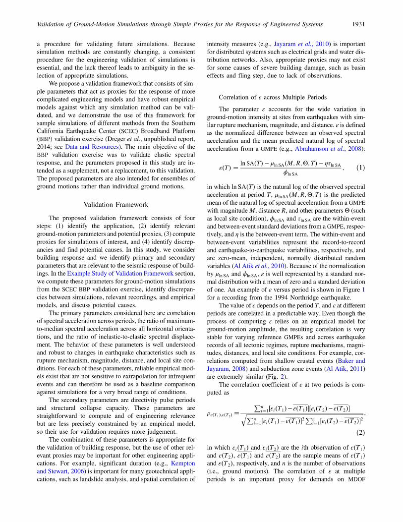
in which ln SA�T� is the natural log of the observed spectralacceleration at period T, μln SA�M;R;Θ; T� is the predictedmean of the natural log of spectral acceleration from a GMPEwith magnitudeM, distance R, and other parameters Θ (suchas local site condition), ϕln SA and τln SA are the within-eventand between-event standard deviations from a GMPE, respec-tively, and η is the between-event term. The within-event andbetween-event variabilities represent the record-to-recordand earthquake-to-earthquake variabilities, respectively, andare zero-mean, independent, normally distributed randomvariables (Al Atik et al., 2010). Because of the normalizationby μln SA and ϕln SA, ε is well represented by a standard nor-mal distribution with a mean of zero and a standard deviationof one. An example of ε versus period is shown in Figure 1for a recording from the 1994 Northridge earthquake.

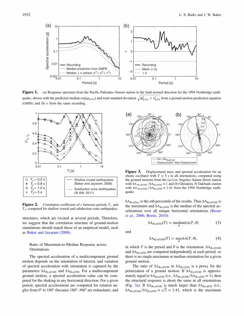
The value of ε depends on the period T, and ε at differentperiods are correlated in a predictable way. Even though theprocess of computing ε relies on an empirical model forground-motion amplitude, the resulting correlation is verystable for varying reference GMPEs and across earthquakerecords of all tectonic regimes, rupture mechanisms, magni-tudes, distances, and local site conditions. For example, cor-relations computed from shallow crustal events (Baker andJayaram, 2008) and subduction zone events (Al Atik, 2011)are extremely similar (Fig. 2).

The correlation coefficient of ε at two periods is com-puted as

ρε�T1�;ε�T2� �Pn

i�1�εi�T1�− ε�T1��εi�T2�− ε�T2��Pni�1�εi�T1�− ε�T1��2

Pni�1�εi�T2�− ε�T2��2

q ;

�2�in which εi�T1� and εi�T2� are the ith observation of ε�T1�and ε�T2�, ε�T1� and ε�T2� are the sample means of ε�T1�and ε�T2�, respectively, and n is the number of observations(i.e., ground motions). The correlation of ε at multipleperiods is an important proxy for demands on MDOF

Validation of Ground-Motion Simulations through Simple Proxies for the Response of Engineered Systems 1931

structures, which are excited at several periods. Therefore,we suggest that the correlation structure of ground-motionsimulations should match those of an empirical model, suchas Baker and Jayaram (2008).

Ratio of Maximum-to-Median Response acrossOrientations

The spectral acceleration of a multicomponent groundmotion depends on the orientation of interest, and variationof spectral acceleration with orientation is captured by theparameters SARotD100 and SARotD50. For a multicomponentground motion, a spectral acceleration value can be com-puted for the shaking in any horizontal direction. For a givenperiod, spectral accelerations are computed for rotation an-gles from 0° to 180° (because 180°–360° are redundant), and

SARotDnn is the nth percentile of the results. Thus SARotD100 isthe maximum and SARotD50 is the median of the spectral ac-celerations over all unique horizontal orientations (Booreet al., 2006; Boore, 2010):

SARotD50�T� � medianθ

SA�T; θ� �3�and

SARotD100�T� � maxθ

SA�T; θ�; �4�in which T is the period and θ is the orientation. SARotD100

and SARotD50 are computed independently at each period, sothere is no single maximum or median orientation for a givenground motion.

The ratio of SARotD100 to SARotD50 is a proxy for thepolarization of a ground motion. If SARotD100 is approxi-mately equal to SARotD50 (i.e., SARotD100=SARotD50 ≈ 1), thenthe structural response is about the same in all orientations(Fig. 3a). If SARotD100 is much larger than SARotD50 (i.e.,SARotD100=SARotD50 ≈

��2

p� 1:41, which is the maximum

(a) (b)

0.01 0.1 1 100.001

0.01

0.1

1

10

Period [s]

Spe

ctra

l acc

eler

atio

n [g

]

RecordingMedian prediction from GMPEMedian ± σ (where σ 2 = φ2 + τ 2)

0.01 0.1 1 10

−2

−1

0

1

2

Period [s]

ε

RecordingMean (= 0)± σ

Figure 1. (a) Response spectrum from the Pacific Palisades–Sunset station in the fault-normal direction for the 1994 Northridge earth-

quake, shown with the predicted median exp�μln SA� and total standard deviation��ϕ2ln SA � τ2ln SA

qfrom a ground-motion prediction equation

(GMPE) and (b) ε from the same recording.

0.01 0.1 1 100

0.2

0.4

0.6

0.8

1

ρ T 1, T

2

T1 [s]

= 0.2 s = 0.8 s = 1.2 s = 3 s

T2

T2

T2T2

Shallow crustal earthquakes (Baker and Jayaram, 2008)

Subduction zone earthquakes (Al Atik, 2011)

Figure 2. Correlation coefficient of ε between periods T1 andT2, computed for shallow crustal and subduction zone earthquakes.

0.2

0.4

0.6

0.8

1

30°

210°

60°

240°

90°

270°

120°

300°

150°

330°

180° 0°

SA / SADisplacement / Max Displacement

RotD100

(a) (b)

0.2

0.4

0.6

0.8

1

30°

210°

60°

240°

90°

270°

120°

300°

150°

330°

180° 0°

Figure 3. Displacement trace and spectral acceleration for anelastic oscillator with T � 5 s in all orientations, computed usingthe ground motions from the (a) Los Angeles–Saturn Street stationwith SA RotD100 =SARotD50 ≈ 1 and (b) Glendora–N Oakbank stationwith SA RotD100 =SARotD50 ≈ 1:41 from the 1994 Northridge earth-quake.

1932 L. S. Burks and J. W. Baker

possible ratio), then the structural response is polarized inone orientation (Fig. 3b).

The median SARotD100=SARotD50 ratio from a suite ofground-motion recordings has a very stable relationship withperiod and is not dependent on magnitude, distance, or localsite conditions. This ratio is important for predictions ofstructural behavior, particularly for 3D structural models,which respond in all orientations. Therefore, simulationsshould have ratios consistent with empirical models (e.g.,Beyer and Bommer, 2006; Shahi and Baker, 2013) (Fig. 4).

Ratio of Inelastic-to-Elastic Displacement

Engineers typically design a structure assuming that itwill behave inelastically during a large earthquake, andtherefore the inelastic relative to elastic behavior of an SDOFoscillator is an important proxy for the behavior of real struc-tures. One common way to quantify the difference betweeninelastic and elastic structural behavior is the ratio of the dis-placement of a bilinear inelastic oscillator Sdi, to an elasticoscillator Sde (see Fig. 5 for force–displacement curves). Thisratio depends on the period T and the strength reduction fac-tor Rμ, which is the force required for the oscillator to remainelastic (Fe) over the yield force Fy or, equivalently, Sde overthe yield displacement dy (Chopra, 2001).

The dependence of Sdi=Sde on T and Rμ is well under-stood from empirical data. In general, the mean ratio isgreater than one at short periods and increases with Rμ, andit is close to one at periods around 1 s where the equal dis-placement rule applies (Veletsos and Newmark, 1960). Inorder for ground-motion simulations with a given elasticspectrum to provide a reliable estimate of inelastic structuralbehavior, their inelastic-to-elastic displacement ratio shouldmatch empirical models, such as Tothong and Cornell(2006), which assumes a bilinear oscillator with α � 0:05and only depends on earthquake magnitude in addition to Tand Rμ (Fig. 6). Instead of using the true Rμ, which depends

on Sde and therefore cannot be known before an earthquakeoccurs, Tothong and Cornell (2006) use the predicted medianreduction factor, Rμ � Sde=dy, in which Sde is the medianprediction from a GMPE.

Some empirical models provide a direct prediction ofSdi at a specific Rμ, such as Bozorgnia et al. (2010), but de-pend on many parameters (e.g., rupture mechanism, magni-tude, distance, local site conditions, etc.) and may or may notextrapolate well to infrequent events such as large magnitudesand short distances. In contrast, the ratio of inelastic-to-elasticdisplacement is more stable with changes in earthquake andsite conditions than Sdi alone (Miranda, 2000). Also, in engi-neering applications the elastic spectrum is often specified bythe design procedure, so the behavior of an inelastic oscillatorrelative to an elastic one is a more representative proxy fortypical engineering analysis. Therefore, we use Tothong andCornell (2006), which predict the mean ratio of Sdi=Sde, forlater comparisons.

Other Ground-Motion Parameters

Other properties, such as directivity pulses and collapsecapacity, are important for engineering applications but arenot well constrained by empirical data and are more sensitiveto changes in earthquake scenario and structural parameters.Therefore, these properties are not considered definitive forvalidation but are described and applied to example ground-motion simulations.

Directivity Pulses. Directivity pulses are a double-sidedvelocity pulse caused by constructive interference of seismicwaves as a rupture propagates along a fault. They tend tooccur at sites that are far from the epicenter, but close to thefault, and are strongest in the fault-normal direction. Thesepulses amplify structural response at long periods and are

Period [s]

Rot

D10

0S

A/ S

AR

otD

50

Beyer and Bommer (2006)

Shahi and Baker (2013)

0.01 0.1 1 101

1.1

1.2

1.3

1.4

Figure 4. Empirical models for the geometric mean ratio ofSARotD100 to SARotD50. The Beyer and Bommer empirical modelreports SARotD100=SAGMRotI50, in which SAGMRotI50 is the medianof the geometric mean of spectral accelerations in a direction basedon a single period (Boore et al., 2006) but is corrected toSARotD100=SARotD50 here using Boore (2010).

00

Fe

Fy

dy Sde Sdi

R = Fe / Fyµ

R = Sde / dyµ

Relative displacement

Late

ral f

orce

K

Elastic oscillator

Bilinear inelastic oscillator

αK

Figure 5. Force–displacement behavior of a bilinear inelasticand an elastic oscillator, in which K is the elastic stiffness (whichrelates to the period T), α is the strain hardening ratio, Fy is the yieldforce, Fe is the elastic force, dy is the yield displacement, Sde is thedisplacement of the elastic oscillator, Sdi is the displacement of theinelastic oscillator, and Rμ is the strength reduction factor.


thus a serious design concern for structures located close to afault (Somerville et al., 1997; Somerville, 2003).

Because theory suggests that pulse period is closely re-lated to the rise time of slip on the fault and the logarithm ofrise time is proportional to magnitude (Somerville, 1998;Somerville et al., 1999), empirical models for pulse periodtypically follow a lognormal distribution for which the meanvalues are a function of earthquake magnitude (e.g., Bray andRodriguez-Marek, 2004; Shahi and Baker, 2011). Theseempirical models are based on historical ground-motion re-cordings, from which pulse periods can be estimated usingwavelet analysis (e.g., Baker, 2007), zero crossings (e.g., Brayand Rodriguez-Marek, 2004), or velocity spectra (e.g.,Alavi and Krawinkler, 2001). However, because there arefew recordings of large magnitude earthquakes at the shortdistanceswhere directivity ismost likely to occur, it is difficultto claim that these models provide a complete description ofdirectivity pulses. In fact, ground-motion simulations may beable to provide a more accurate characterization of directivitypulses and near-fault ground motions because they capturefinite-fault geometry and source-to-site path characteristics.But some cases may exist where it is useful to compare thepulse characteristics of simulations to empirical models.

Structural Collapse Capacity. The collapse capacity of astructure is the ground-motion intensity level that causes itto lose stability and collapse. Onemethod to compute collapsecapacity is an incremental dynamic analysis (IDA), and thefinal result is a collapse fragility curve that defines the prob-ability of collapse given a ground-motion intensity (Ibarra andKrawinkler, 2005). An IDA is performed by incrementallyscaling up a single ground motion until collapse occurs.The IDA is repeated for a set of ground motions to get a prob-abilistic description of collapse and is typically performed us-ing the full nonlinear MDOF model of a structure of interest.

Because collapse capacity is highly dependent on struc-tural properties such as period, peak-to-yield-displacement

ratio, postpeak stiffness, and collapse mechanism (Zareianet al., 2010), it is a difficult parameter to validate. Therefore,we propose the use of three generic nonlinear SDOF modelsto act as a proxy for more complicated MDOF models. Theproposed SDOFs have periods of T � 0:3, 0.8, and 2 s butthe same relative force–drift behavior, and they are represen-tative of midrise concrete frame buildings (Fig. 7, inwhich Fy=W � 0:198, Fc=W � 0:216, αc � −0:1, anddc=dy � 4). Their hysteretic behavior is represented by apeak-oriented model with negligible cyclic deterioration(e.g., Ibarra and Krawinkler, 2005). For ground motions,we suggest using an existing set of recordings, then selectinga set of simulations with comparable elastic response spectra.The spectral equivalence controls for differences in elasticresponse, so discrepancies in the resulting collapse capacitymust be due to other, less obvious properties of the groundmotions. The collapse capacity can be computed for each

0 5 100.7

1

1.5

2

2.5

Sdi

/ S

de

(a)

0 5 100.7

1

1.5

2

2.5

Sdi

/ S

de

(b)T = 0.3 sT = 0.6 sT = 0.8 sT = 2 s

Strength reduction factor, Rµ Strength reduction factor, Rµ

Magnitude = 6 Magnitude = 7

Figure 6. Empirical model for the ratio of the displacement of a bilinear inelastic to an elastic oscillator Sdi=Sde for an earthquake withmagnitude (a) 6 and (b) 7, as a function of period T and predicted median reduction factor Rμ � Sde=dy, in which Sde is the median predictionfrom a GMPE (Tothong and Cornell, 2006).

0 0.02 0.04 0.06 0.08 0.10

0.05

0.1

0.15

0.2

0.25

dy /H dc /H

Fy /W

K = M · (2π/T)2

αc ·K

Drift ratio

For

ce /

Wei

ght

αs ·K

Fc /W

Figure 7. Force–drift backbone curve for the proposed struc-tural system, in which T is period, H is height, M is mass, W isweight, Fy is yield force, Fc is peak force, αc is postpeak stiffness,dc is displacement at peak force, dy is yield displacement, and K isstiffness.


SDOF using each set of ground motions, and the collapsecapacities for recordings can be compared to simulations.

Structural collapse capacity is essential for capturing thehighly nonlinear behavior of structures, which plays a largerole in seismic risk assessment, but collapse capacity can bedifficult to compute and is highly dependent on structuralmodeling choices and ground-motion selection. These chal-lenges make it a complicated and possibly less robust vali-dation metric for ground-motion simulations, but certainlynot any less important.

Example Study of Validation Framework

This section presents examples of the proposed parame-ters evaluated using sample ground-motion simulations. Foreach parameter, we attempt to show an example that matchesthe empirical model and an example that deviates. Becausemany were implemented without these checks in mind, the in-tent of this section is not to judge the simulations, but rather todemonstrate the computation of these parameters and discusspossible outcomes. Some of the simulation methods may beeasily improved in future implementations on the SCEC BBP.

Example of Ground-Motion Simulations

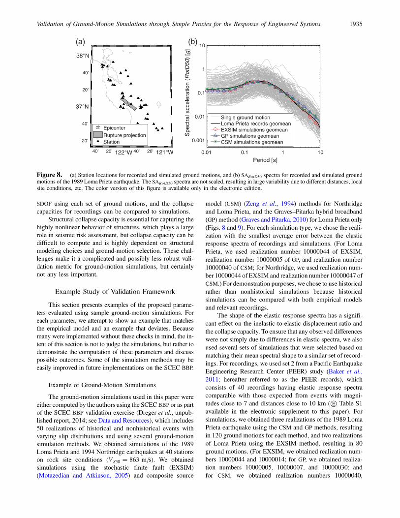
The ground-motion simulations used in this paper wereeither computed by the authors using the SCECBBP or as partof the SCEC BBP validation exercise (Dreger et al., unpub-lished report, 2014; see Data and Resources), which includes50 realizations of historical and nonhistorical events withvarying slip distributions and using several ground-motionsimulation methods. We obtained simulations of the 1989Loma Prieta and 1994 Northridge earthquakes at 40 stationson rock site conditions (VS30 � 863 m=s). We obtainedsimulations using the stochastic finite fault (EXSIM)(Motazedian and Atkinson, 2005) and composite source

model (CSM) (Zeng et al., 1994) methods for Northridgeand Loma Prieta, and the Graves–Pitarka hybrid broadband(GP) method (Graves and Pitarka, 2010) for Loma Prieta only(Figs. 8 and 9). For each simulation type, we chose the reali-zation with the smallest average error between the elasticresponse spectra of recordings and simulations. (For LomaPrieta, we used realization number 10000044 of EXSIM,realization number 10000005 of GP, and realization number10000040 of CSM; for Northridge, we used realization num-ber 10000044 of EXSIM and realization number 10000047 ofCSM.) For demonstration purposes, we chose to use historicalrather than nonhistorical simulations because historicalsimulations can be compared with both empirical modelsand relevant recordings.

The shape of the elastic response spectra has a signifi-cant effect on the inelastic-to-elastic displacement ratio andthe collapse capacity. To ensure that any observed differenceswere not simply due to differences in elastic spectra, we alsoused several sets of simulations that were selected based onmatching their mean spectral shape to a similar set of record-ings. For recordings, we used set 2 from a Pacific EarthquakeEngineering Research Center (PEER) study (Baker et al.,2011; hereafter referred to as the PEER records), whichconsists of 40 recordings having elastic response spectracomparable with those expected from events with magni-tudes close to 7 and distances close to 10 km (Ⓔ Table S1available in the electronic supplement to this paper). Forsimulations, we obtained three realizations of the 1989 LomaPrieta earthquake using the CSM and GP methods, resultingin 120 ground motions for each method, and two realizationsof Loma Prieta using the EXSIM method, resulting in 80ground motions. (For EXSIM, we obtained realization num-bers 10000044 and 10000014; for GP, we obtained realiza-tion numbers 10000005, 10000007, and 10000030; andfor CSM, we obtained realization numbers 10000040,

40’ 20’ 122°W 40’ 20’ 121°W

20’

40’

37°N

20’

40’

38°N

(a)

EpicenterRupture projectionStation

0.01 0.1 1 10

0.001

0.01

0.1

1

10

Period [s]

Spe

ctra

l acc

eler

atio

n (R

otD

50)

[g]

(b)

Single ground motionLoma Prieta records geomeanEXSIM simulations geomeanGP simulations geomeanCSM simulations geomean

Figure 8. (a) Station locations for recorded and simulated ground motions, and (b) SARotD50 spectra for recorded and simulated groundmotions of the 1989 Loma Prieta earthquake. The SARotD50 spectra are not scaled, resulting in large variability due to different distances, localsite conditions, etc. The color version of this figure is available only in the electronic edition.


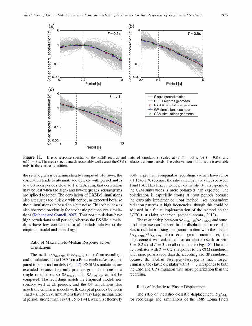
10000017, and 10000038.) From those 120 or 80, we se-lected 40 that best matched the mean of scaled spectra ofthe PEER records (Fig. 10 and Ⓔ Tables S2–S4). The meanspectrum of the selected simulations reasonably matches themean spectrum of recordings scaled at several periods(Fig. 11), but the standard deviation varies (Fig. 12). Forfuture validation purposes, we suggest using any set of re-cordings as long as the mean of scaled elastic spectramatches the simulations that are being validated.

Finally, we use hybrid broadband simulations from twosets of earthquake scenarios computed using SCEC BBPversion 11.2.3, with the GP method for the rupture generatorand low-frequency seismogram, and the San Diego StateUniversity method (Mai et al., 2010) for high-frequencyseismogram and site response. The first set contains 10 real-

izations of a magnitude 7 earthquake on the Hayward faultwith 12 stations, each located 1 km from the fault withVS30 � 500 m=s (Fig. 13). The second set contains 10 real-izations of a magnitude 7 earthquake on the San Andreasfault, with similar rupture geometry to the 1989 Loma Prietaearthquake, and 12 stations located 1 km from the surfaceprojection of the fault with VS30 � 500 m=s (Fig. 14). Eachset of scenarios contains 120 near-fault ground-motionsimulations and is used for the evaluation of pulse periods.

Correlation of ε across Multiple Periods

Here we compare the statistics of ε from empirical mod-els to recordings and simulations of the 1989 Loma Prietaearthquake. In this example, the between-event term in equa-tion (1) is constant for a given period and cancels out becauseall ground motions are from the same event. The standarddeviation of ε is expected to equal one at all periods becauseof the normalization in equation (1). The recordings and CSMsimulations have a standard deviation close to one at all peri-ods, the EXSIM simulations have a small standard deviationat all periods (≈0:24 to 0.64), and the GP simulations have asmall standard deviation at periods shorter than 1 s (≈0:36 to0.64) but close to 1 at longer periods (Fig. 15). At short peri-ods, the EXSIM and GP simulation methods are very similar,resulting in similar behavior of ε. For GP simulations, thehigh- and low-frequency seismograms are spliced togetherat 1 s, so the change in standard deviation at this period sug-gests a lack of variability in the high-frequency simulationprocess, previously observed by Seyhan et al. (2013).

Correlations of ε at select periods are shown in Figure 16.In general, the recordings follow the empirical modelswhereas the simulations do not. Even the correlation of ε forthe CSM simulations differs from empirical models, despitehaving a reasonable standard deviation of ε. The GP simula-tions match the empirical model between periods around 1 sand less than 0.1 s and between periods longer than 1 s where

0.01 0.1 1 100.001

0.01

0.1

1

10

Period [s]

Sca

led

spec

tral

acc

eler

atio

n [g

]

Single ground motionPEER records geomeanEXSIM simulations geomeanGP simulations geomeanCSM simulations geomean

Figure 10. Elastic response spectra scaled at T � 0:8 s for set 2from a Pacific Earthquake Engineering Research Center (PEER)study (Baker et al., 2011; hereafter referred to as the PEER records)and several sets from different simulation methods selected basedon their match with the mean spectral shape of the PEER records.The color version of this figure is available only in the electronicedition.

20’ 119ºW 40’ 20’ 118ºW 40’

40’

34ºN

20’

40’

35ºN

(a)

EpicenterRupture projectionStation

0.01 0.1 1 100.001

0.01

0.1

1

10

Period [s]

Spe

ctra

l acc

eler

atio

n (R

otD

50)

[g]

(b)

Single ground motionNorthridge records geomeanEXSIM simulations geomeanCSM simulations geomean

Figure 9. (a) Station locations for recorded and simulated ground motions, and (b) SARotD50 spectra for recorded and simulated groundmotions of the 1994 Northridge earthquake. The SARotD50 spectra are not scaled, resulting in large variability due to different distances, localsite conditions, etc. The color version of this figure is available only in the electronic edition.


the seismogram is deterministically computed. However, thecorrelation tends to attenuate too quickly with period and islow between periods close to 1 s, indicating that correlationmay be lost when the high- and low-frequency seismogramsare spliced together. The correlation of EXSIM simulationsalso attenuates too quickly with period, as expected becausethese simulations are based onwhite noise. This behavior wasalso observed previously for stochastic point-source simula-tions (Tothong andCornell, 2007). The CSM simulations havehigh correlations at all periods, whereas the EXSIM simula-tions have low correlations at all periods relative to theempirical model and recordings.

Ratio of Maximum-to-Median Response acrossOrientations

The median SARotD100 to SARotD50 ratios from recordingsand simulations of the 1989 Loma Prieta earthquake are com-pared to empirical models (Fig. 17). EXSIM simulations areexcluded because they only produce ground motions in asingle orientation, so SARotD50 and SARotD100 cannot becomputed. The recordings match the empirical models rea-sonably well at all periods, and the GP simulations alsomatch the empirical models well, except at periods between1 and 4 s. The CSM simulations have a very large median ratioat periods shorter than 1 s (≈1:35 to 1.41), which is effectively

50% larger than comparable recordings (which have ratios≈1:16 to 1.30) because the ratio can only have values between1 and 1.41. This large ratio indicates that structural response tothe CSM simulations is more polarized than expected. Thepolarization is especially strong at short periods becausethe currently implemented CSM method uses nonrandomradiation patterns at high frequencies, though this could beadjusted in a future implementation of the method on theSCEC BBP (John Anderson, personal comm., 2013).

The relationship between SARotD100=SARotD50 and struc-tural response can be seen in the displacement trace of anelastic oscillator. Using the ground motion with the medianSARotD100=SARotD50 from each ground-motion set, thedisplacement was calculated for an elastic oscillator withT � 0:2 s and T � 3 s in all orientations (Fig. 18). The elas-tic oscillator with T � 0:2 s responds to the CSM simulationwith more polarization than the recording and GP simulationbecause the median SARotD100=SARotD50 is much larger.Similarly, the elastic oscillator with T � 3 s responds to boththe CSM and GP simulation with more polarization than therecording.

Ratio of Inelastic-to-Elastic Displacement

The ratio of inelastic-to-elastic displacement, Sdi=Sde,for recordings and simulations of the 1989 Loma Prieta

0.1 0.3 1 20.02

0.1

1

6

Period [s]

Sca

led

spec

tral

acc

eler

atio

n [g

]

(a)

0.4 0.8 1 50.02

0.1

1

6

Period [s]

Sca

led

spec

tral

acc

eler

atio

n [g

]

(b)

Single ground motionPEER records geomeanEXSIM simulations geomeanGP simulations geomeanCSM simulations geomean

2 3 100.02

0.1

1

6

Period [s]

Sca

led

spec

tral

acc

eler

atio

n [g

]

(c)

T = 0.3s T = 0.8s

T = 3 s

Figure 11. Elastic response spectra for the PEER records and matched simulations, scaled at (a) T � 0:3 s, (b) T � 0:8 s, and(c) T � 3 s. The mean spectra match reasonably well except the CSM simulations at long periods. The color version of this figure is availableonly in the electronic edition.


earthquake is compared to an empirical model at multipleperiods (Fig. 19). At T � 1:6 s, the recordings and all sim-ulations match the empirical model, but at T � 0:8 s, GP andCSM simulations have a mean ratio that is about 11% and5%, respectively, larger than the empirical model. The inelas-tic behavior of an SDOF oscillator depends strongly on the

elastic response at longer periods because the effectivenatural period lengthens as the SDOF behaves nonlinearly(Iwan, 1980). Therefore, the discrepancy in Sdi=Sde at differ-ent periods can be at least partially explained by the differ-ence in relative shape of the scaled response spectra(Fig. 20). Scaled at T � 1:6 s, the mean response spectrum

0.1 0.3 1 20

0.2

0.4

0.6

0.8

Period [s]

σ o

f ln

SA

sca

led

[g]

T = 0.3s

(a)

0.4 0.8 1 50

0.2

0.4

0.6

0.8

Period [s]

σ o

f ln

SA

sca

led

[g]

T = 0.8s

(b)

PEER recordsEXSIM simulationsGP simulationsCSM simulations

2 3 100

0.2

0.4

0.6

0.8

Period [s]

σ o

f ln

SA

sca

led

[g]

T = 3 s

(c)

Figure 12. Standard deviation of the natural log of the scaled elastic response spectra for the PEER records and matched simulations,scaled at (a) T � 0:3 s, (b) T � 0:8 s, and (c) T � 3 s. The color version of this figure is available only in the electronic edition.

45’ 30’ 15’ 122°W 45’ 30’ 12’

24’

36’

48’

38ºN

12’

(a)Rupture projectionStation

0.1 1 100.01

0.1

1

10

Period [s]

Spe

ctra

l acc

eler

atio

n [g

]

(b)

Single simulationSimulations geomeanMedian prediction from GMPE

Figure 13. The set of Hayward scenario simulations: (a) station locations and (b) response spectra in the north–south direction. This setcontains 10 realizations of a magnitude 7 earthquake, with 12 stations located 1 km from the fault.


is similar for the recordings and all simulations at periodsslightly longer than 1.6 s; however, scaled at T � 0:8 s,the mean of GP and CSM simulations is larger than the re-cordings at longer periods, leading to a larger inelastic dis-placement and inelastic-to-elastic displacement ratio.

To control for the spectral shape, we compare the inelas-tic-to-elastic displacement ratio of the PEER records andmatched simulations to an empirical model at multiple peri-ods (Fig. 21). Now that the mean spectral shape is similar,Sdi=Sde for the PEER records and all matched simulations atT � 0:8 s agrees with the empirical model. Yet discrepan-cies remain at T � 0:3 s and T � 3 s; for example, the ratioof EXSIM simulations is about 17% and 6% (respectively,)below recordings on average, even though their mean spectraare similar (see the mean spectra in Fig. 11). Also, atT � 0:3 s, the ratio of GP simulations is about 9% belowrecordings on average, even though the mean spectrum issimilar. These discrepancies may be due to differences in the

standard deviation of the scaled response spectra (recallFig. 12). At T � 0:3 s, both the EXSIM and GP simulationshave standard deviations smaller than recordings at periodslonger than 0.3 s, leading to smaller Sdi=Sde. At T � 3 s, theEXSIM simulations have a smaller standard deviation,whereas the GP simulations have a standard deviation thatmatches the PEER records, leading to a small Sdi=Sde for theEXSIM simulations and an Sdi=Sde that matches the PEERrecords for the GP simulations.

Other Ground-Motion Parameters

Directivity Pulses. Here we compare the distribution ofpulse periods from the sets of scenarios on the Hayward andSan Andreas faults with two empirical models (Bray and Ro-driguez-Marek, 2004; Shahi and Baker, 2011). Pulse periodswere extracted from the east–west component of all groundmotions using wavelet analysis (Baker, 2007). Even thoughall earthquake scenarios are magnitude 7 with stationslocated 1 km from the fault, the San Andreas simulations aredominated by pulse periods between 1 and 2 s, whereas theHayward simulations are dominated by longer pulse periodsbetween 4 and 5 s (Fig. 22). The distribution of pulse periodsfrom the San Andreas scenario is more similar to the empiri-cal models than the Hayward scenario.

In general, the validation of pulse characteristics againstempirical models is often not feasible because it requires alarge sample of pulses—and therefore an even larger sampleof ground-motion simulations. Because many simulationapplications do not produce a large sample of near-faultground motions, such as simulations of historical events, itcan be difficult to statistically analyze their pulse properties.However, for the validation of historical simulations, we candirectly compare the location and pulse periods that occurredin the actual event to the simulation of the event. BecauseNorthridge contains more pulse-like ground motions thanLoma Prieta (using wavelet analysis; e.g., Baker, 2007), wecompare recordings to simulations in the north–south

24’ 12’ 122ºW 48’ 36’ 24’

40’

50’

37°N

10’

20’

(a)

0.1 1 100.001

0.01

0.1

1

10

Period [s]

Spe

ctra

l acc

eler

atio

n [g

]

(b)

Single simulationSimulations geomeanMedian prediction from GMPE

Rupture projection

Station

Intersection of rupture plane with surface

Figure 14. The set of San Andreas scenario simulations: (a) station locations and (b) response spectra in the north–south direction. Thisset contains 10 realizations of a magnitude 7 earthquake, with 12 stations located 1 km from the surface projection of the rupture.

0.01 0.1 1 100

0.5

1

1.5

Period [s]

σ ε

Loma Prieta records

EXSIM simulations

GP simulations

CSM simulations

Figure 15. Standard deviation of ε for the recordings and sim-ulations of the 1989 Loma Prieta earthquake, shown with the ex-pected standard deviation of one. The color version of thisfigure is available only in the electronic edition.


direction of the Northridge earthquake. The recordings con-tain seven pulses, CSM simulations contain six pulses, and theEXSIM simulations contain only one pulse. The location ofpulses tends to be in the northeast corner of the fault projection

for the recordings and both sets of simulations (Fig. 23). Thepulse periods for the CSM simulations are similar to record-ings and range from1 to 2.5 s, and the only pulse period for theEXSIM simulations is 2 s (Fig. 24). Results from GP simula-tions are omitted here because of space constraints.

Structural Collapse Capacity. We computed the collapsecapacity using an IDA of the three proposed SDOF structuresusing the PEER records and matched simulations (Fig. 25).Because the mean and standard deviation of the elastic spec-tra scaled at T � 0:8 s are similar for all ground motions, themedian collapse capacity of the SDOF with T � 0:8 s is alsosimilar for all ground motions (all simulations are within 6%of the recordings). In contrast, the standard deviation of theelastic spectra scaled at T � 0:3 s is small for GP simula-tions, leading to a 12% increase in the median collapsecapacity for the SDOF with T � 0:3 s, which is an unconser-vative estimate. Similarly, the standard deviation of theEXSIM elastic spectra scaled at T � 2 s is small, again lead-ing to a 12% increase in the median collapse capacity for theSDOF with T � 2 s.

The results shown in Figure 25 are empirical cumulativedistribution functions (not fragility functions) based on 40

0.01 0.1 1 100

0.2

0.4

0.6

0.8

1

ρT

1, T

2

T2 = 0.2s(a)

0.01 0.1 1 100

0.2

0.4

0.6

0.8

1T2 = 0.8s(b)

0.01 0.1 1 100

0.2

0.4

0.6

0.8

1

T1 [s]

ρT

1, T

2

T2 = 1.2s(c)

0.01 0.1 1 100

0.2

0.4

0.6

0.8

1

T1 [s]

T2 = 3s

(d)

Loma Prieta recordsEXSIM simulationsGP simulationsCSM simulationsBaker & Jayaram (2008)Al Atik (2011)

Figure 16. Correlation of ε for recordings and simulations of the 1989 Loma Prieta earthquake, shown with an empirical model forshallow crustal earthquakes (Baker and Jayaram, 2008) and results from subduction zone earthquakes (Al Atik, 2011) at (a) T2 � 0:2 s,(b) T2 � 0:8 s, (c) T2 � 1:2 s, and (d) T2 � 3 s. The color version of this figure is available only in the electronic edition.

0.01 0.1 1 101

1.1

1.2

1.3

1.4

Period [s]

SA

Rot

D10

0 / S

AR

otD

50

Loma Prieta records medianGP simulations medianCSM simulations medianBeyer and Bommer (2006)Shahi and Baker (2013)

Figure 17. Ratio of SARotD100 to SARotD50 from empirical mod-els and the median ratio from recordings and simulations of the1989 Loma Prieta earthquake. The color version of this figure isavailable only in the electronic edition.


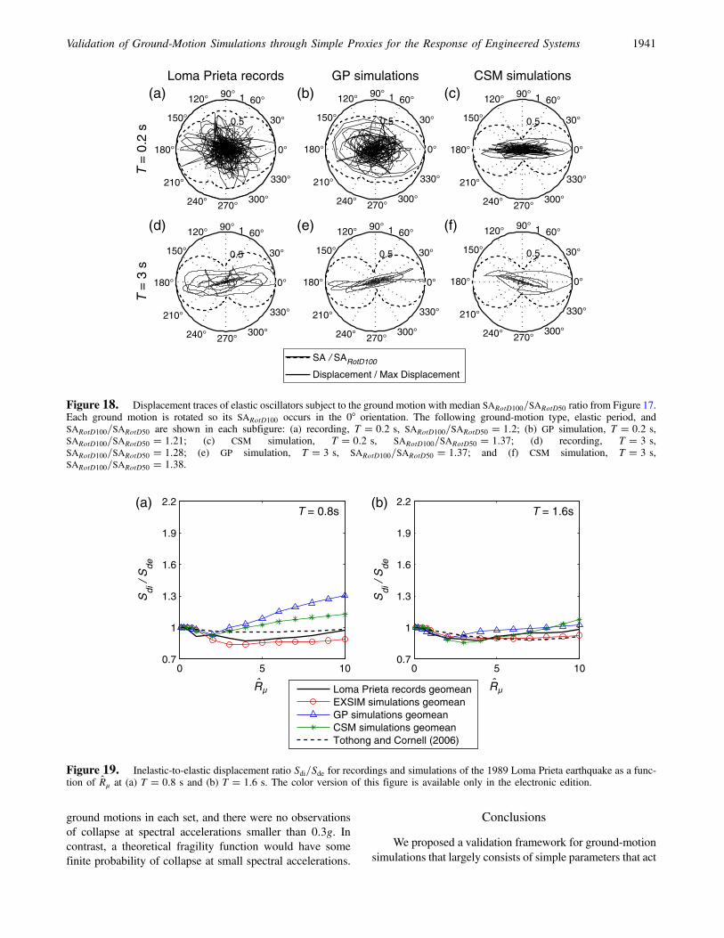
ground motions in each set, and there were no observationsof collapse at spectral accelerations smaller than 0:3g. Incontrast, a theoretical fragility function would have somefinite probability of collapse at small spectral accelerations.

Conclusions

We proposed a validation framework for ground-motionsimulations that largely consists of simple parameters that act

0.5

1

30°

210°

60°

240°

90°

270°

120°

300°

150°

330°

180° 0°

Loma Prieta records

T =

0.2

s

(a)GP simulations

(b)CSM simulations

(c)

T =

3 s

(d) (e) (f)

SA / SARotD100

Displacement / Max Displacement

0.5

1

30°

210°

60°

240°

90°

270°

120°

300°

150°

330°

180° 0°

0.5

1

30°

210°

60°

240°

90°

270°

120°

300°

150°

330°

180° 0°

0.5

1

30°

210°

60°

240°

90°

270°

120°

300°

150°

330°

180° 0°

0.5

1

30°

210°

60°

240°

90°

270°

120°

300°

150°

330°

180° 0°

0.5

1

30°

210°

60°

240°

90°

270°

120°

300°

150°

330°

180° 0°

Figure 18. Displacement traces of elastic oscillators subject to the ground motion with median SARotD100=SARotD50 ratio from Figure 17.Each ground motion is rotated so its SARotD100 occurs in the 0° orientation. The following ground-motion type, elastic period, andSARotD100=SARotD50 are shown in each subfigure: (a) recording, T � 0:2 s, SARotD100=SARotD50 � 1:2; (b) GP simulation, T � 0:2 s,SARotD100=SARotD50 � 1:21; (c) CSM simulation, T � 0:2 s, SARotD100=SARotD50 � 1:37; (d) recording, T � 3 s,SARotD100=SARotD50 � 1:28; (e) GP simulation, T � 3 s, SARotD100=SARotD50 � 1:37; and (f) CSM simulation, T � 3 s,SARotD100=SARotD50 � 1:38.

0 5 100.7

1

1.3

1.6

1.9

2.2

Sdi

/ S

de

T = 0.8s(a)

0 5 100.7

1

1.3

1.6

1.9

2.2

Sdi

/ S

de

T = 1.6s

(b)

Loma Prieta records geomeanEXSIM simulations geomeanGP simulations geomeanCSM simulations geomeanTothong and Cornell (2006)

Rµ Rµ

Figure 19. Inelastic-to-elastic displacement ratio Sdi=Sde for recordings and simulations of the 1989 Loma Prieta earthquake as a func-tion of Rμ at (a) T � 0:8 s and (b) T � 1:6 s. The color version of this figure is available only in the electronic edition.


0.4 0.8 1 5

0.1

1

Period [s]

Sca

led

spec

tral

acc

eler

atio

n [g

]

(a)

0.8 1 1.6 10

0.1

1

Period [s]

Sca

led

spec

tral

acc

eler

atio

n [g

]

(b)

Single ground motionLoma Prieta records geomeanEXSIM simulations geomeanGP simulations geomeanCSM simulations geomean

Figure 20. Elastic response spectra for recordings and simulations of the 1989 Loma Prieta earthquake scaled at (a) T � 0:8 s and(b) T � 1:6 s. The color version of this figure is available only in the electronic edition.

0 5 100.7

1

1.3

1.6

1.9

2.2

Sdi

/ S

de

T = 0.3s(a)

0 5 100.7

1

1.3

1.6

1.9

2.2

Sdi

/ S

de

T = 0.8s(b)

0 5 100.7

1

1.3

1.6

1.9

2.2

Sdi

/ S

de

T = 3s

(c)

Rµ Rµ

Rµ

PEER records geomeanEXSIM simulations geomeanGP simulations geomeanCSM simulations geomeanTothong and Cornell (2006)

Figure 21. Inelastic-to-elastic displacement ratio Sdi=Sde for PEER records and matched simulations as a function of Rμ at (a) T � 0:3 s,(b) T � 0:8 s, and (c) T � 3:0 s. The color version of this figure is available only in the electronic edition.


as proxies for the response of more complicated engineeredsystems and have robust empirical models that are insensitiveto changes in earthquake scenario. The validation frameworkconsisted of four steps: (1) identify application, (2) identifyproxies, (3) compute proxies, and (4) identify discrepanciesand potential causes. We also provided an example of theframework for building response using several differentsimulation methods from the SCEC BBP, including EXSIM,the GP method, and CSM.

First, we discussed the correlation of ε across periods,the ratio of SARotD100 to SARotD50, and the ratio of inelastic-to-elastic displacement because these parameters have robustempirical models against which simulations from a broadrange of conditions can be compared. Correlation of ε cap-tures the relative spectral response at different periods, mak-ing it an important proxy for demands on MDOF structures.From the example simulations used in this study, we saw thatCSM simulations overestimated the correlation, whereasEXSIM simulations underestimated it. For GP simulations,

0 1 2 3 4 5 6 70

0.05

0.1

0.15

0.2

0.25

0.3

0.35

0.4

Tp [s]

Pro

babi

lity

dens

ity

San Andreas ScenariosHayward ScenariosShahi and Baker (2011)Bray and Rodriguez−Marek (2004)

Figure 22. Histogram of pulse period Tp in the east–west di-rection for the Hayward and San Andreas scenario simulations com-pared with two empirical models.

Station without pulseStation with pulseEpicenterRupture projection

40’

20’

40’

35°N

34°N

20’ 40’ 20’ 40’ 119°W 118°W 20’ 40’ 20’ 40’ 119°W 118°W 20’ 40’ 20’ 40’ 119°W 118°W

(a) (b) (c)

Figure 23. Map of pulse locations in the north–south direction during the 1994 Northridge earthquake for (a) recordings, (b) CSMsimulations, and (c) EXSIM simulations.

Tp [s]

Fre

quen

cy o

f obs

erva

tions CSM simulations

Northridge records

0 1 2 3 40

0.2

0.4

0.6

0.8

1

Tp [s]

Fre

quen

cy o

f obs

erva

tions

(a) (b)

0 1 2 3 40

0.2

0.4

0.6

0.8

1

EXSIM simulationsNorthridge records

Figure 24. Histogram of pulse periods in the north–south direction from the 1994 Northridge earthquake of (a) CSM simulations and(b) EXSIM simulations compared with recordings.


correlations matched empirical models at long periods forwhich simulations are deterministically computed but wereunderestimated at short periods for which simulations arestochastically generated. The ratio of SARotD100 to SARotD50

is a proxy for the polarization of ground motions and isimportant for 3D structures. In our examples, the simulationstend to be more polarized than recordings at long periods, butthe simulation methods give varying results at short periods.The inelastic-to-elastic displacement ratio is a proxy for theresponse of nonlinear structures, and most structures are de-signed to behave nonlinearly in a large earthquake. This ratiois highly dependent on the mean and standard deviation ofthe elastic response spectra at longer periods because thestructure’s period effectively lengthens as the structurebehaves nonlinearly, and we observed that this ratio fromrecordings and simulations is similar when the mean andstandard deviation match.

Then, we discussed other parameters such as directivityfeatures and collapse capacity of idealized structures becausethey are important for engineering applications, althoughthey are not as well constrained by empirical models and arethus more difficult to validate. Because relatively few record-ings exist that contain directivity pulses, empirical modelsmay not be as reliable as simulations in predicting pulse

periods. However, in the example simulations, we observedthat directivity parameters such as presence of a pulse andpulse period vary significantly between simulation methods,making it difficult to know which is physically correct.Collapse capacity is important for the evaluation of highlynonlinear structures and for seismic risk assessments, butit is highly dependent on ground-motion selection and struc-tural modeling choices. Therefore, in validating this param-eter, great care must be taken to choose ground-motionrecordings and simulations with similar elastic spectra, andthe same structural model must be evaluated for all ground-motion sets. To demonstrate the validation framework, wecomputed the collapse capacity of idealized structural mod-els and observed that the median collapse capacity from sim-ulations was within 12% of recordings.

In general, we observed that each simulation methodmatched some empirical models and not others, indicatingthe value of checking the accuracy of all relevant ground-motion parameters. The list of ground-motion parametersproposed in this study is not exhaustive but covers someproxies that are important to the seismic response of build-ings for a variety of reasons. For other engineering ap-plications (e.g., landslide analysis, distributed systems,etc.), the use of other relevant proxies is important; and,

0 0.5 1 1.5 20

0.2

0.4

0.6

0.8

1

SA(T=0.3s) collapse [g]

Cum

ulat

ive

prob

abili

ty

(a)

0 1 2 30

0.2

0.4

0.6

0.8

1

SA(T=0.8s) collapse [g]

Cum

ulat

ive

prob

abili

ty

(b)

0 1 2 3 40

0.2

0.4

0.6

0.8

1

SA(T=2s) collapse [g]

Cum

ulat

ive

prob

abili

ty

(c)PEER recordsEXSIM simulationsGP simulationsCSM simulations

Figure 25. Empirical cumulative distribution function of structural collapse capacity using PEER records and matched simulations onnonlinear SDOF structures with (a) T � 0:3 s, (b) T � 0:8 s, and (c) T � 2 s. The color version of this figure is available only in theelectronic edition.


for applications where no relevant proxies exist (e.g., buildingdamage due to basin effects or fling step), a different valida-tion strategy is necessary. Further research may be necessaryto quantify how similar simulations should be to an empiricalmodel to ensure reliable results, but in many cases, the vali-dation framework presented here is consistent and can provideconfidence in simulations for appropriate applications.

Data and Resources

Simulations were either obtained from the SouthernCalifornia Earthquake Center (SCEC) Broadband Platform(BBP) validation exercise (Dreger et al., 2014) or computedusing SCEC BBP version 11.2.3, which is available for down-load at http://scec.usc.edu/scecpedia/Broadband_Platform(last accessed July 2013). Recordings were obtained from thePacific Earthquake Engineering Research Center NextGeneration Attenuation database at http://peer.berkeley.edu/peer_ground_motion_database (last accessed July 2013).

Acknowledgments

Thanks to Robert Graves, Kim Olsen, and John Anderson for helpfulinterpretations of the ground-motion simulation methods and to Linda AlAtik for sharing ε correlation data for subduction zone earthquakes. Thisresearch was supported by the Southern California Earthquake Center(SCEC) and the National Science Foundation (NSF) under NSF Grant Num-ber ACI 1148493. SCEC is funded by NSF Cooperative AgreementEAR-0529922 and U.S. Geological Survey (USGS) Cooperative Agreement07HQAG0008. The SCEC Contribution Number for this paper is 1793. Anyopinions, findings, and conclusions or recommendations expressed in thismaterial are those of the authors and do not necessarily reflect the viewsof the sponsors.

References

Aagaard, B. T., T. M. Brocher, D. Dolenc, D. Dreger, R. W. Graves,S. Harmsen, S. Hartzell, S. Larsen, and M. L. Zoback (2008).Ground-motion modeling of the 1906 San Francisco earthquake, partI: Validation using the 1989 Loma Prieta earthquake, Bull. Seismol.Soc. Am. 98, no. 2, 989–1011.

Abrahamson, N., G. Atkinson, D. Boore, Y. Bozorgnia, K. Campbell,B. Chiou, I. M. Idriss, W. Silva, and R. Youngs (2008). Comparisonsof the NGA ground-motion relations, Earthq. Spectra 24, no. 1, 45–66.

Al Atik, L. (2011). Correlation of spectral acceleration values for subductionand crustal models, in COSMOS Technical Session, Emeryville,California, 13 pp., http://www.cosmos‑eq.org/technicalsession/TS2011/presentations/2011_alatik.pdf (last accessed July 2013).

Al Atik, L., N. Abrahamson, J. J. Bommer, F. Scherbaum, F. Cotton, andN. Kuehn (2010). The variability of ground-motion prediction modelsand its components, Seismol. Res. Lett. 81, no. 5, 794–801.

Alavi, B., and H. Krawinkler (2001). Effects of near-fault ground motions onframe structures, Technical Report 138, Blume EarthquakeEngineering Center, Stanford, California.

Anderson, J. G. (2004). Quantitative measure of the goodness-of-fit ofsynthetic seismograms, in 13th World Conference on EarthquakeEngineering, Vancouver, B.C., Canada, Vol. 243, Earthquake Engi-neering Research Institute, 1–14.

Baker, J. W. (2007). Quantitative classification of near-fault ground motionsusing wavelet analysis, Bull. Seismol. Soc. Am. 97, no. 5, 1486–1501.

Baker, J. W., and N. Jayaram (2008). Correlation of spectral accelerationvalues from NGA ground motion models, Earthq. Spectra 24,no. 1, 299–317.

Baker, J. W., T. Lin, S. K. Shahi, and N. Jayaram (2011). New ground mo-tion selection procedures and selected motions for the PEER transpor-tation research program, Technical Report PEER 2011/03, PacificEarthquake Engineering Research Center, Berkeley, California.

Bazzurro, P., B. Sjoberg, and N. Luco (2004). Post-elastic response ofstructures to synthetic ground motions, Technical Report PEER1G00 Addendum 2, Pacific Earthquake Engineering Research Center,Berkeley, California.

Beresnev, I. A., and G. M. Atkinson (1997). Modeling finite-fault radiationfrom the ωn spectrum, Bull. Seismol. Soc. Am. 87, no. 1, 67–84.

Beyer, K., and J. J. Bommer (2006). Relationships between median valuesand between aleatory variabilities for different definitions of the hori-zontal component of motion, Bull. Seismol. Soc. Am. 96, no. 4A,1512–1522.

Boore, D. M. (1983). Stochastic simulation of high-frequency groundmotions based on seismological models of the radiated spectra, Bull.Seismol. Soc. Am. 73, no. 6A, 1865–1894.

Boore, D. M. (2010). Orientation-independent, nongeometric-mean mea-sures of seismic intensity from two horizontal components of motion,Bull. Seismol. Soc. Am. 100, no. 4, 1830–1835.

Boore, D. M., J. Watson-Lamprey, and N. A. Abrahamson (2006).Orientation-independent measures of ground motion, Bull. Seismol.Soc. Am. 96, no. 4A, 1502–1511.

Bozorgnia, Y., M. M. Hachem, and K. W. Campbell (2010). Ground motionprediction equation (“attenuation relationship”) for inelastic responsespectra, Earthq. Spectra 26, no. 1, 1–23.

Bray, J. D., and A. Rodriguez-Marek (2004). Characterization of forward-directivity ground motions in the near-fault region, Soil Dynam.Earthq. Eng. 24, no. 11, 815–828.

Chopra, A. K. (2001). Dynamics of Structures: Theory and Applications toEarthquake Engineering, Second Ed., Prentice Hall, Upper SaddleRiver, New Jersey.

Der Kiureghian, A., and J. Crempien (1989). An evolutionary model forearthquake ground motion, Struct. Saf. 6, no. 24, 235–246.

Frankel, A. (2009). A constant stress-drop model for producing broadbandsynthetic seismograms: Comparison with the Next Generation Attenu-ation relations, Bull. Seismol. Soc. Am. 99, no. 2A, 664–680.

Galasso, C., F. Zareian, I. Iervolino, and R. W. Graves (2012). Validation ofground-motion simulations for historical events using SDoF systems,Bull. Seismol. Soc. Am. 102, no. 6, 2727–2740.

Galasso, C., P. Zhong, F. Zareian, I. Iervolino, and R. W. Graves (2013).Validation of ground-motion simulations for historical events usingMDoF systems, Earthq. Eng. Struct. Dynam. 42, no. 9, 1395–1412.

Graves, R. W., and A. Pitarka (2010). Broadband ground-motionsimulation using a hybrid approach, Bull. Seismol. Soc. Am. 100,no. 5A, 2095–2123.

Hartzell, S., M. Guatteri, P. M. Mai, P.-C. Liu, and M. Fisk (2005).Calculation of broadband time histories of ground motion, part II:Kinematic and dynamic modeling using theoretical Green’s functionsand comparison with the 1994 Northridge earthquake, Bull. Seismol.Soc. Am. 95, no. 2, 614–645.

Hartzell, S., S. Harmsen, A. Frankel, and S. Larsen (1999). Calculation ofbroadband time histories of ground motion: Comparison of methodsand validation using strong-ground motion from the 1994 Northridgeearthquake, Bull. Seismol. Soc. Am. 89, no. 6, 1484–1504.

Ibarra, L. F., and H. Krawinkler (2005). Global collapse of frame structuresunder seismic excitations, Technical Report 152, Blume EarthquakeEngineering Center, Stanford, California.

Iervolino, I., F. De Luca, and E. Cosenza (2010). Spectral shape-based as-sessment of SDOF nonlinear response to real, adjusted and artificialaccelerograms, Eng. Struct. 32, no. 9, 2776–2792.

Iwan, W. D. (1980). Estimating inelastic response spectra from elastic spec-tra, Earthq. Eng. Struct. Dynam. 8, no. 4, 375–388.

Jayaram, N., and N. Shome (2012). A statistical analysis of the response oftall buildings to recorded and simulated ground motions, in 15th WorldConference on Earthquake Engineering, Lisbon, Portugal, 24–28 Sep-tember 2012, 1–10.


http://scec.usc.edu/scecpedia/Broadband_Platform



http://peer.berkeley.edu/peer_ground_motion_database

http://peer.berkeley.edu/peer_ground_motion_database

http://www.cosmos-eq.org/technicalsession/TS2011/presentations/2011_alatik.pdf





Jayaram, N., J. Park, P. Bazzurro, and P. Tothong (2010). Spatial correlationbetween spectral accelerations using simulated ground-motion timehistories, in 9th U.S. National and 10th Canadian Conference onEarthquake Engineering, Toronto, Canada, 25–29 July 2010, 1–10.

Jurkevics, A., and T. J. Ulrych (1978). Representing and simulating strongground motion, Bull. Seismol. Soc. Am. 68, no. 3, 781–801.

Kempton, J. J., and J. P. Stewart (2006). Prediction equations for significantduration of earthquake ground motions considering site andnear-source effects, Earthq. Spectra 22, no. 4, 985–1013.

Kristekova, M., J. Kristek, P. Moczo, and S. M. Day (2006). Misfit criteriafor quantitative comparison of seismograms, Bull. Seismol. Soc. Am.96, no. 5, 1836–1850.

Mai, P. M., W. Imperatori, and K. B. Olsen (2010). Hybrid broadbandground-motion simulations: Combining long-period deterministicsynthetics with high-frequency multiple S-to-S backscattering, Bull.Seismol. Soc. Am. 100, no. 5A, 2124–2142.

Miranda, E. (2000). Inelastic displacement ratios for structures on firm sites,J. Struct. Eng. 126, no. 10, 1150–1159.

Mobarakeh, A., F. Rofooei, and G. Ahmadi (2002). Simulation of earth-quake records using time-varying Arma (2,1) model, Prob. Eng. Mech.17, no. 1, 15–34.

Motazedian, D., and G. M. Atkinson (2005). Stochastic finite-fault modelingbased on a dynamic corner frequency, Bull. Seismol. Soc. Am. 95,no. 3, 995–1010.

Olsen, K. B., and J. E. Mayhew (2010). Goodness-of-fit criteria for broad-band synthetic seismograms, with application to the 2008 M 5.4Chino Hills, California, earthquake, Seismol. Res. Lett. 81, no. 5,715–723.

Pousse, G., L. F. Bonilla, F. Cotton, and L. Margerin (2006). Nonstationarystochastic simulation of strong ground motion time histories includingnatural variability: Application to the K-Net Japanese database, Bull.Seismol. Soc. Am. 96, no. 6, 2103–2117.

Schmedes, J., R. Archuleta, and D. Lavallee (2010). Correlation of earth-quake source parameters inferred from dynamic rupture simulations,J. Geophys. Res. 115, no. B3, doi: 10.1029/2009JB006689.

Seyhan, E., J. P. Stewart, and R. W. Graves (2013). Calibration of a semi-stochastic procedure for simulating high-frequency ground motions,Earthq. Spectra 29, no. 4, 1495–1519.

Shahi, S. K., and J. W. Baker (2011). An empirically calibrated frameworkfor including the effects of near-fault directivity in probabilistic seismichazard analysis, Bull. Seismol. Soc. Am. 101, no. 2, 742–755.

Shahi, S. K., and J. W. Baker (2013). NGA-West2 models for ground-motiondirectionality, Technical Report PEER 2013/10, Pacific EarthquakeEngineering Research Center, Berkeley, California.

Somerville, P. (1998). Development of an improved representation of nearfault ground motions, in Seminar on Utilization of Strong-MotionData, Oakland, California, 1–20.

Somerville, P. (2003). Magnitude scaling of the near fault rupture directivitypulse, Phys. Earth Planet. In. 137, no. 1, 1–12.

Somerville, P., K. Irikura, R. Graves, S. Sawada, D. Wald, N. Abrahamson,Y. Iwasaki, T. Kagawa, N. Smith, and A. Kowada (1999). Character-izing crustal earthquake slip models for the prediction of strong groundmotion, Seismol. Res. Lett. 70, no. 1, 59–80.

Somerville, P., N. F. Smith, R. W. Graves, and N. A. Abrahamson (1997).Modification of empirical strong ground motion attenuation relationsto include the amplitude and duration effects of rupture directivity,Seismol. Res. Lett. 68, no. 1, 199–222.

Star, L. M., J. P. Stewart, and R. W. Graves (2011). Comparison of groundmotions from hybrid simulations to NGA prediction equations,Earthq. Spectra 27, no. 2, 331–350.

Tothong, P., and C. A. Cornell (2006). An empirical ground-motion attenu-ation relation for inelastic spectral displacement, Bull. Seismol. Soc.Am. 96, no. 6, 2146–2164.

Tothong, P., and C. A. Cornell (2007). Probabilistic seismic demand analysisusing advanced ground motion intensity measures, attenuation rela-tionships, and near-fault effects, Technical Report PEER 2006/11,Pacific Earthquake Engineering Research Center, Berkeley, California.

Veletsos, A., and N. Newmark (1960). Effect of inelastic behavior on theresponse of simple systems to earthquake motions, in 2nd WorldConference on Earthquake Engineering, Tokyo, Japan, 895–912.

Zareian, F., H. Krawinkler, L. Ibarra, and D. Lignos (2010). Basic conceptsand performance measures in prediction of collapse of buildings underearthquake ground motions, Struct. Design Tall Sp. Buildings 19,nos. 1/2, 167–181.

Zeng, Y., J. G. Anderson, and G. Yu (1994). A composite source model forcomputing realistic synthetic strong ground motions, Geophys. Res.Lett. 21, no. 8, 725–728.

Stanford UniversityBlume Earthquake Engineering CenterBuilding 540, Room 207Stanford, California [email protected]

(L.S.B.)

Stanford University473 Via Ortega, Room 283Stanford, California 94305

(J.W.B.)

Manuscript received 24 October 2013;Published Online 15 July 2014


http://dx.doi.org/10.1029/2009JB006689

by lynne s. burks and jack w. baker - stanford...

Documents