CAE Working Paper #04-06

Regional Inflation During the French Revolution

by

Levon Barseghyan

Francesca Molinari

and

François Velde

May 2004

.

Regional In�ation During The French Revolution

Levon Barseghyan Francesca Molinari François Velde

December 15, 2000

Abstract

Shortly after the Revolution of 1789 France experienced a period of major hyper-

in�ation, which lasted until 1796, when the French government abolished the paper

money and returned to the specie. In 1798 the French government ordered the local

authorities in all departments to construct the aggregate price index. Even though

similar in trend, these price series display striking di¤erences both in level and short

run dynamics. Some of these di¤erences are undoubtedly caused by the absence of

a uniform rule for constructing the price indices, and possibly are magni�ed by such

distortionary factors as the laws of maximum, the heavy concentration of military con-

tracts in particular locations, and the di¤erent taxation schemes. However, level of

economic integration in 18th century France had a major impact on the price evo-

lution during the Revolution. In this paper, using di¤erent proxies for a measure of

economic distance, we show that price formation among �close�departments displayed

signi�cantly higher correlation than the one among �distant�departments.

1 Introduction

Shortly after the Revolution of 1789 France experienced a period of major hyperin�ation,

which lasted until 1796, when the French government abolished the paper money and re-

turned to the specie. In 1798 the French government ordered the local authorities in all

1

departments to construct the aggregate price index to be used in restructuring the govern-

ment debt, as well as in recalculating other obligations made in Assignats (paper money).

Even though similar in trend, these price series display striking di¤erences both in level and

short run dynamics. Some of these di¤erences are undoubtedly caused by the absence of a

uniform rule for constructing the price indices, and possibly are magni�ed by such distor-

tionary factors as the laws of maximum, the heavy concentration of military contracts in

particular locations, and the di¤erent taxation schemes. However, we think that the main

reason behind these variations is the level of economic integration in 18th century France.

This paper is an attempt to show that integration indeed mattered and close economic

ties between departments vastly contributed to similar in�ation patterns among them. In

particular, using di¤erent proxies for a measure of economic distance, we show that price

formation among �close� departments displayed signi�cantly higher correlation than the

one among �distant� departments. This result is robust to di¤erent model speci�cations,

including one which endogenizes similarities in industrial structure of departments.

The rest of the paper is organized as follows. In Section 2 we present the overall economic

conditions on the eve and during the French Revolution, and the origins of Assignats, while

in Section 3 we discuss the avialable data. Section 4 introduces the model we use to study the

price series, describes our main �ndings, and shows their robustness. Section 5 concludes.

2

departments to construct the aggregate price index to be used in restructuring the govern-

ment debt, as well as in recalculating other obligations made in Assignats (paper money).

Even though similar in trend, these price series display striking di¤erences both in level and

short run dynamics. Some of these di¤erences are undoubtedly caused by the absence of a

uniform rule for constructing the price indices, and possibly are magni…ed by such distor-

tionary factors as the laws of maximum, the heavy concentration of military contracts in

particular locations, and the di¤erent taxation schemes. However, we think that the main

reason behind these variations is the level of economic integration in 18th century France.

This paper is an attempt to show that integration indeed mattered, and close economic

ties between departments vastly contributed to similar in‡ation patterns among them. In

particular, using di¤erent proxies for a measure of economic distance, we show that price

formation among “close” departments displayed signi…cantly higher correlation than the

one among “distant” departments. This result is robust to di¤erent model speci…cations,

including one which endogenizes similarities in industrial structure of departments.

The rest of the paper is organized as follows. In Section 2 we present the overall economic

conditions on the eve and during the French Revolution, and the origins of Assignats, while

in Section 3 we discuss the avialable data. Section 4 introduces the model we use to study the

price series, describes our main …ndings, and shows their robustness. Section 5 concludes.

2 State of the economy: the origins of in‡ation

2.1 Economic Conditions

In 1789, urban population constituted slightly less than one-quarter of the total population

(Harris [10], p3). Agriculture still was the main occupation; but at the outbreak of the

Revolution, it was in a deplorable condition: undercapitalization, low average crop yields

(only 2/3 of the average crop yields in England), absence of well developed small farm

infrastructure (Harris [10], p3). Also, a few subsequent years of bad harvests contributed to

the unfavorable conditions in the subsistence markets.

2

Many scholars agree that the main reason for these grave conditions in rural sector seems

to be an extremely ill designed tax system. The amount of taille, the heaviest direct tax, to

be paid by a particular household was left on the discretion of the tax collectors, and was

determined almost solely based on the appearances. In this conditions many peasants found

more bene…cial not to appear wealthy in order to avoid the tax burden. The eager to avoid

the taille was so high, that many households became indeed poor:

They [the peasants] did not dare to procure for themselves the number of

animals necessary for good farming; they used to cultivate their …elds in a poor

way so as to pass as poor, which is what they eventually became; they pretended

that it was too hard to pay in order to avoid paying too much: payments that

were inevitably slow were made still slower; they took no pleasure or enjoyment

in their food, housing or dress; their days passed in deprivation and sorrow (from

the cahier de doleances -o¢cial list of grievances- of the Third Estate in the

baillage of Nemours, cited in Aftalion [1]).

During the Revolution the situation did not improve signi…cantly. Although most of

Church’ and emigre’s land was expropriated and put on sale, with very little or no down-

payment required, the majority of the rural population did not have enough resources to take

advantage of this opportunity. Due to in‡ation, controlled prices, and requisitions (especially

during the Terror), they were left with essentially no capital to buy out their debts to the

landowners and purchase a land. It is true though, that in the beginning of the Revolution

the tax burden itself was reduced by the inability of the new authorities to collect taxes,

and that afterwards it was reduced through the reorganization of the tax system in a more

equitable and simple scheme. However, this was not su¢cient to substantially change the

overall economic conditions of the rural sector.

Manufacturing was not in better conditions. The majority of French industries still were

in a rudimentary state, with textiles contributing more than 50% of the nation’s industrial

output (Aftalion [1], p34). Only very few industries, like mining and metalworking, had

3

advanced forms of organization and a stable work force. The majority of city dwellers was

employed in services and textile. Wars and civil unrest alone did not play a major role in

the collapse of the manufacturing sector right before and during the French Revolution. As

P. Butel ([5] p37) notes:

[...] though the productive potential of some towns was undermined by mili-

tary operations or civil disturbances, such destruction was quite limited in time

and space.

The core of the problems was rather in the dramatic reduction of the working capital of

merchants and manufactures through the sharp rise in costs, obligatory government contracts

(payment for which was usually done in depreciating paper money), price controls, loss of

export markets, diversion of resources to military purposes and the heavy burden of taxation.

With continuing war, sea blockade, and in‡ation, the industrial output fell sharply till 1796.

Even though it started to recover after that, by 1799-1800 it was at most 50-60% of the 1789

level.

2.2 Taxes and Circulating Currency on the Eve of the Revolution

One of the most critical problems faced by the Ancien Regime and afterwards by the Estates-

General was the constant excess of expenditure over the revenues. In fact budget de…cit and

inadequacy of …scal system were so dominant in the pre-Revolutionary France, that some

authors consider them “as the Direct cause of French Revolution” (see for example Aftalion

[1], p11).

The Fiscal System of the Ancien Regime was both complicated and, more importantly,

inequitable. It consisted of numerous royal and seigniorial taxes, along with payments to

the Church. As we have mentioned above, the most evil tax, in economic sense, was the

taille. It originally was levied to …nance wars, and therefore was imposed only on the civil

population. The determination of taille liabilities was left solely on the discretion of the

tax collectors, who did not have any accurate measure of the wealth of taxpayers. In these

4

conditions, nobility was essentially exempt from taille, as the only estimate of their wealth

was the amount they declared themselves.

The other direct taxes included capitation tax and vingtieme. These taxes as well were

based on the real means of taxpayers. But similarly to the taille payments, nobility was quite

able to avoid, or signi…cantly reduce, their obligations by not disclosing their wealth. Clergy

was in even better position, since in theory they were determining the amount of “gifts” to

the Crown on a voluntary basis. Consequently, the Royal tax burden was put almost solely

on the Third Estate. Needless to say, the Third Estate was also responsible for contributions

to nobility, clergy, and for the hole system of indirect taxes.

The most painful indirect tax was the gabelle (tax on salt). Its amount varied signi…cantly

from region to region, accounting for around 15% of the total Royal taxes. During the Ancien

Regime there were several attempts to conduct a …scal reform and bring tax duties to one

uni…ed and relatively fair ground. However, nobility and clergy successfully defeated all

such proposals, and kept their tax privileges. (Ex post, nobility and clergy could have been

better o¤ accepting a …scal system more fair and less painful for the Third Estate, since that

may have prevented the Revolution, and therefore loss of essentially all their land and other

property.)

The pre-Revolutionary France faced another serious problem: the disappearance of the

currency. Political instability, worsening economic conditions, and disparities in exchange

rates caused hoarding and exportation of the specie. While the decrease in the amount of

circulating currency remains unclear, Harris [10] reports numerous evidence on “partial or

even complete loss of metallic money”. It is important to mention that prices in this period

did not respond to this monetary contraction, putting the real side of the economy even in

worse conditions. In August 1788 the Royal Treasury attempted to introduce new interest

bearing paper notes. However, because of the general incon…dence in the existing regime

and the memories of Law’s paper money, the wave of overwhelming disagreement caused the

Government to abandon the issuance.

5

2.3 Revenues of the Revolution and infeasibility of the …scal re-

form

As Revolution “had been made precisely in order to oppose taxation” (Aftalion [1], p.68), the

new Treasury faced exactly the same political opposition to a …scal mechanism which could

provide enough revenues for government to operate. In June 14, 1789 a decree declaring all

taxes illegal was passed. Although within two months it was reversed, the public opposition

to taxes was very high. In March of 1790 the salt tax (gabelle) was abandoned, and in

November the Contribution Fonciere, the corner stone of the new tax system, was passed.

The latter was based on a unique direct tax, levied on all social groups, and proportional

to the wealth of the taxpayers. However the reaction against taxation persisted through

1791. It took almost two years till an improved administration of local municipalities led

to signi…cant tax revenues. By the end of 1792, the central authorities received around 175

million livres in taxes, which constituted roughly 16% of total expenditure. From that period

on taxes were collected quite stably, but the …scal revenues never constituted more then 25%

of the total expenditures. While more dramatic tax schedules and forced contribution were

proposed during the later years of the Revolution, they never brought a signi…cant increase

in the Treasury funds, both because of political opposition and di¢culties in collection. (see

Table Harris1)

Loans, another traditional source of income employed by the Ancien Regime to cover

its de…cits, could not provide signi…cant funds due to administrative impotence, decline in

savings, and most importantly political and economic instability.

Therefore, the only real source of income for the government to cover its growing expen-

ditures was through seignorage. (Indeed, it is almost uniformly agreed by historians that the

Revolution was …nanced almost entirely by Assignats.) Initially, issuance of unbacked paper

money was not possible due to a large political resistance and the unpleasant experience of

the Law’s paper money in the beginning of the century. However, in a situation so di¢cult

that some members of the Assembly even proposed the bankruptcy of the State, the rem-

edy was found rather quickly. By October 1789 many in‡uential politicians like Mireabreu

6

and Talleyrand publicly called upon con…scation of the Church’ land in order to …nance the

budget. The idea quickly evolved into a plan according to which no interest bearing notes

would be issued, later to be used to buy a con…scated land. It is important to note that there

were also sound political reasons behind this plan. The members of the Assembly realized

that the sale of con…scated land to a large group of population would provide wide public

support for the Revolution, since it would create a new class of landowners, whose property

rights would be guaranteed only if the Revolution would survive.

On December 19, 1789 the …rst issue of Assignats in the amount of 400 million livres was

approved. Originally, Assignats were designed as bonds bearing a 5% interest, to be used in

the purchase of nationalized land, and were not legal tender. Emission of another 400 million

livres, this time in small nominations to facilitate circulation and trade, was conducted on

April 17, 1790. At this time Assignats were declared a form of currency, bearing a 3%

interest. In October the interest was abandoned, completing the transformation of Assignats

into currency.

On the face of the increasing expenditures, especially caused by the necessity to …nance

the war, numerous emissions followed. By 1793 Assignats essentially became …at money,

causing a sharp rise in prices and drop in real balances. As the base of in‡ation tax was

threatened, a strict price control, the law of Maximum, was introduced. During 1794 suc-

cesses in the war made impossible the enforcement of restrictions on prices and trade, causing

a new wave of depreciation of Assignats. The law of Maximum o¢cially was abandoned on

December 1794. In 1795 both prices and amount of circulating Assignats were growing

exponentially.

By the February of 1796, when the printing presses for Assignats were broken, the total

amount of the Assignats in circulation was about 34-39.000 million, around 85-97 times more

than the …rst emission.

7

3 Data

In 1798, on the request of the Central Government, the local authorities prepared tables of

monthly value of the paper money for the period from 1791 till 1796. (For the …nal year,

when daily changes in prices were signi…cant, the daily data is available). The objective was

to provide a basis for the translation of paper money obligations into metallic equivalents.

The data set used in this paper consists of these price series, collected for all pre-1789

departments. 1 Our analysis spans the period going from January 1791 till February 1796,

for which we have monthly data.

3.1 Non-uniformity in the construction of the price index

departments were given the Treasury prices of the gold and silver. Local authorities had to

combine this information with prices of goods on the local markets to construct the price of

a consumption bundle in terms of Assignats. Goods included in the bundle were precious

metals, land, agricultural products, merchandize, and manufacturing goods. It was advised

from Paris to include in the bundle land, food, and commodities, prices of which were not

controlled during the Maximum period. However, some of the local authorities explicitly

used controlled prices to construct the price index. This of course creates asymmetry in

assessing the value of Assignats across di¤erent regions, since one may with high degree of

certainty expect that inclusion of controlled commodities in the bundle would arti…cially

increase the purchasing power of the paper money. On the other hand, almost all necessities

at some point were rationed or had controlled prices, so it is not clear whether one would

have a representative bundle after excluding these necessities from it.

Also, the price of gold was depressed substantially by the o¢cial propaganda and violence

during the Terror, contributing to increase the value of Assignats. Therefore, depending on

the weight of gold and silver in the consumption bundle used to construct the price indices,

1The data for the 13 Departments which were annexed by France during the war is also available, but

there are doubts regarding the comparability of these price series with the data for the pre-1789 Departments.

8

one may observe substantial di¤erences across the latter. Moreover, prices of goods in

di¤erent departments varied substantially even before the Revolution, so it remains unclear

to what extent di¤erences in the value of a particular bundle were due to in‡ation and

economic turmoil, and not to “true” price di¤erential of elements of the bundle.

A comparison of the price series of the di¤erent departments shows an extremely large

variation both in the level and in the short run dynamics of the value of the Assignats.

Figure A plots di¤erent percentiles, and the mean of 84 pre 1789 French departments. The

di¤erence between the …rst and the nineth deciles at its peak is 32.5% of pre 1790 value,

while the di¤erence between the …rst and the third quantiles at the peak of 16.5% is no less

striking. As Figure B shows, the same magnitude di¤erences are displayed by the in‡ation

rates.

What are the reasons for such diversity? What caused such a wild degree of variation?

Are there any testable hypotheses which can help to explain them?

As mentioned above, some of the variation is due to the non-uniformity in the construc-

tion of these time series. However, one might expect that non-uniformity would primarily

a¤ect the level, but not the growth rate of prices. The other reason for such dramatically

di¤erent price behavior is of course given by the di¤erences in economic structure across the

departments and the level of economic integration between them.

3.2 Diverse economic environment

There are two key factors which determined the economic role of a particular department.

First, we think that location was of particular importance. Geographically closer provinces

should have had more similar, inter-dependent economies than distant ones, due to similar

climate and natural resources, higher trade volume, and often close socio-political environ-

ment. Since agriculture contributed around three quarters of the total GDP, climate was an

important determinant in economic position of counties. Also, di¢culties in transportation

and existence of tari¤s and rent seekers on the boundaries of the departments made trade

9

with close locations more advantageous. Then, it seems reasonable to assume2 that closer

departments had more common industries than far ones. To illustrate the importance of

geographical location in price formation, we plot in Figure C the value of Assignats for …ve

di¤erent regions: North, North-West, North-East, South-West, and South-East. As the …g-

ure illustrates, Assignats had the highest value in the North-Western part of the country,

while the lowest was in the South-Eastern part. The fact that Assignats were valued the

least in the South-Eastern region can be explained by the signi…cant circulation of foreign

currency in that area, and by the subsistence crisis that this region experienced from 1790

till essentially 1798.

Second, we believe that industrial specialization plays an important role in de…ning the

economic conditions of a particular region. This is especially true for economies which

experienced drastic changes over short periods of time. For example, if two di¤erent counties

were highly specialized in the same good, demand for which fell sharply all over the nation

within a very short period of time, one may safely assume that both of these counties would

experience very similar economic changes, including price formation, ‡y of capital and so on.

Indeed, phenomena of such kind were observed. Essentially all cities with ports on the

Atlantic coast were experiencing the same kind of di¢culties during the French Revolution.

Not only the wealth of these cities was signi…cantly undermined by the loss of colonial trade,

but also their economies su¤ered dramatic demand shocks. Industries of ports were developed

during the golden years of colonial expansion, and were almost exclusively export oriented.

As sea blockade became more and more di¢cult to bypass, the manufactures were shut,

leaving more and more city dwellers out of job and means of existence. Francois Crouzet,

among the others, has argued that there was a lasting de-individualization or pastoralization

of large areas, with de…nite shift of capital from trade and industry towards agriculture.

To illustrate the extent of the industrial collapse, Paul Butel considers as an example the

town of Tonneins, which had 1000 ropemakers in 1789 and only 200 in 1800, 1200 workers

employed at a tobacco factory in 1789 but fewer then 200 in 1800.

2Evidence from Table? con…rms that qualitatively this is the case.

10

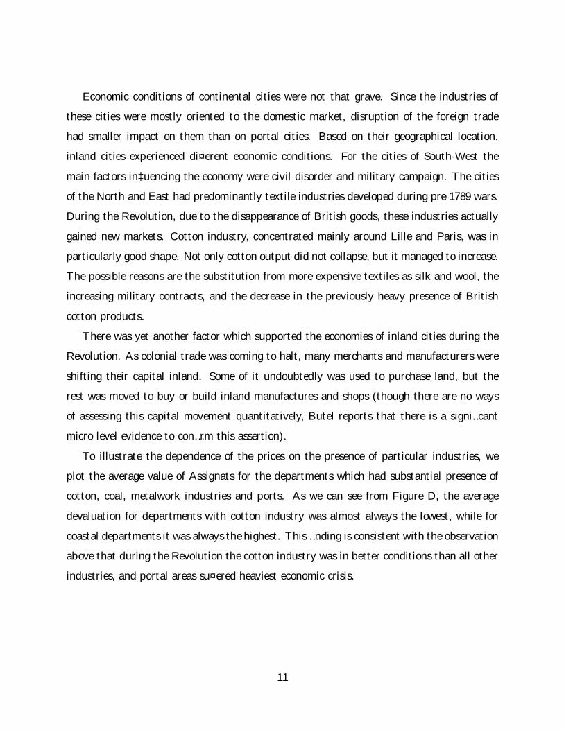
Economic conditions of continental cities were not that grave. Since the industries of

these cities were mostly oriented to the domestic market, disruption of the foreign trade

had smaller impact on them than on portal cities. Based on their geographical location,

inland cities experienced di¤erent economic conditions. For the cities of South-West the

main factors in‡uencing the economy were civil disorder and military campaign. The cities

of the North and East had predominantly textile industries developed during pre 1789 wars.

During the Revolution, due to the disappearance of British goods, these industries actually

gained new markets. Cotton industry, concentrated mainly around Lille and Paris, was in

particularly good shape. Not only cotton output did not collapse, but it managed to increase.

The possible reasons are the substitution from more expensive textiles as silk and wool, the

increasing military contracts, and the decrease in the previously heavy presence of British

cotton products.

There was yet another factor which supported the economies of inland cities during the

Revolution. As colonial trade was coming to halt, many merchants and manufacturers were

shifting their capital inland. Some of it undoubtedly was used to purchase land, but the

rest was moved to buy or build inland manufactures and shops (though there are no ways

of assessing this capital movement quantitatively, Butel reports that there is a signi…cant

micro level evidence to con…rm this assertion).

To illustrate the dependence of the prices on the presence of particular industries, we

plot the average value of Assignats for the departments which had substantial presence of

cotton, coal, metalwork industries and ports. As we can see from Figure D, the average

devaluation for departments with cotton industry was almost always the lowest, while for

coastal departments it was always the highest. This …nding is consistent with the observation

above that during the Revolution the cotton industry was in better conditions than all other

industries, and portal areas su¤ered heaviest economic crisis.

11

4 Econometric Model

The analysis carried on in the previous Sections leads to the conclusion that the non-uniform

economic conditions across the departments of 1790’s France should play a key role in ex-

plaining the striking di¤erences in their price levels and in‡ation rates.

Therefore, to study the relation between the prices of the di¤erent departments, ideally

one would like to construct and test a model of the following type: ¦t+1 = f (¹t;¦t; ECt);

where ¦t is the vector of in‡ation rates across the departments, ¹t is the growth rate of

money, and ECt is a matrix of variables characterizing the economic conditions of the de-

partments. Although we have data regarding the growth rate of money and an indication of

the prevailing industry in a given region, there is no available data to help to quantitatively

assess the economic conditions of the French departments during 1789-1796.

However, we can use the information provided by two proxies of the “similarities” of the

economic conditions between departments.3 These proxies are: their geographic distance,

and the traveling time that one would have employed to go from the center of one department

to the center of another. In the next two Sections we will show the informative power of

such proxies, and present evidence that the “closer” (either geographically or in terms of

traveling distance) two departments are, the more their in‡ation rates4 move similarly.

4.1 Preliminary Analysis of the Data

Given the monthly price levels of the 84 French departments from January 1791 to February

1796, we construct the demeaned in‡ation rates ¼t as follows:

¼t = log

ÃPtPt¡1

!¡ E

"log

ÃPtPt¡1

!#(1)

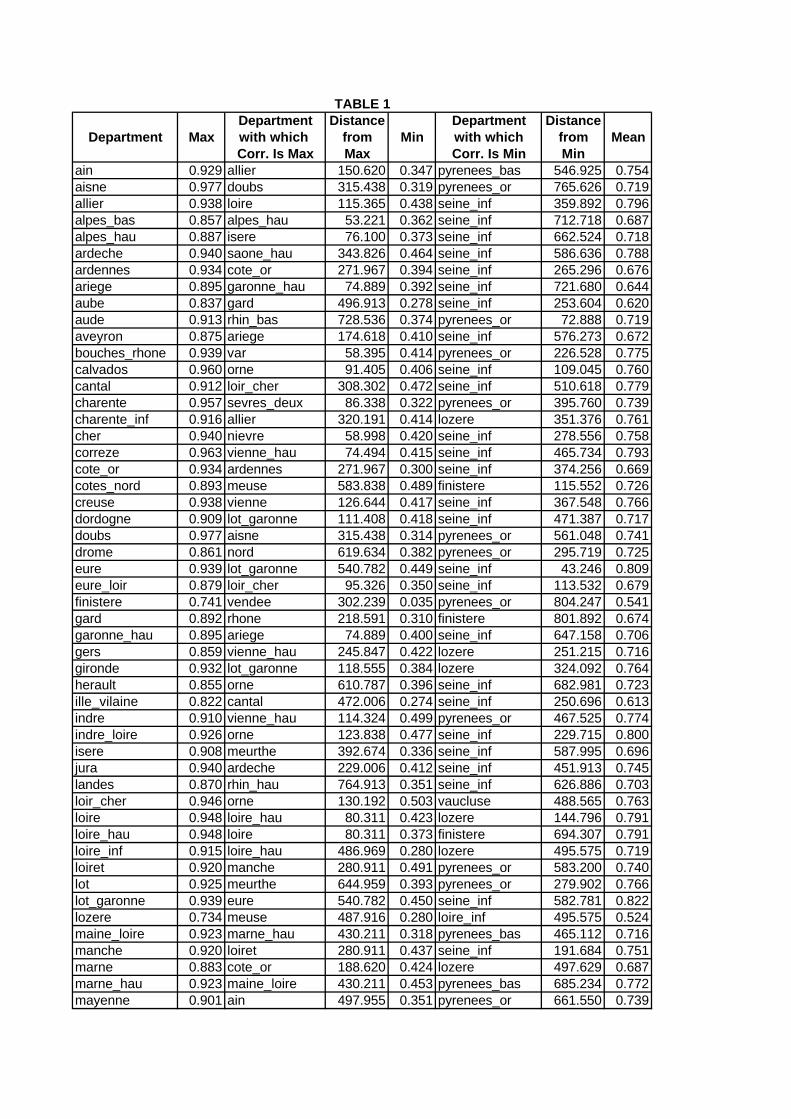
Those in‡ation rates display a strong correlation across departments. As Table 1 reports,

the maximum correlation coe¢cient between ¼jt and ¼it, i; j = 1; : : : ; 84 (i.e. across all

departments) is 0.977, the minimum is 0.035, and the mean is 0.724. This correlation

3Using a technique that we will describe in Section 4.2.4As well as price levels, but we will concentrate on the former.

12

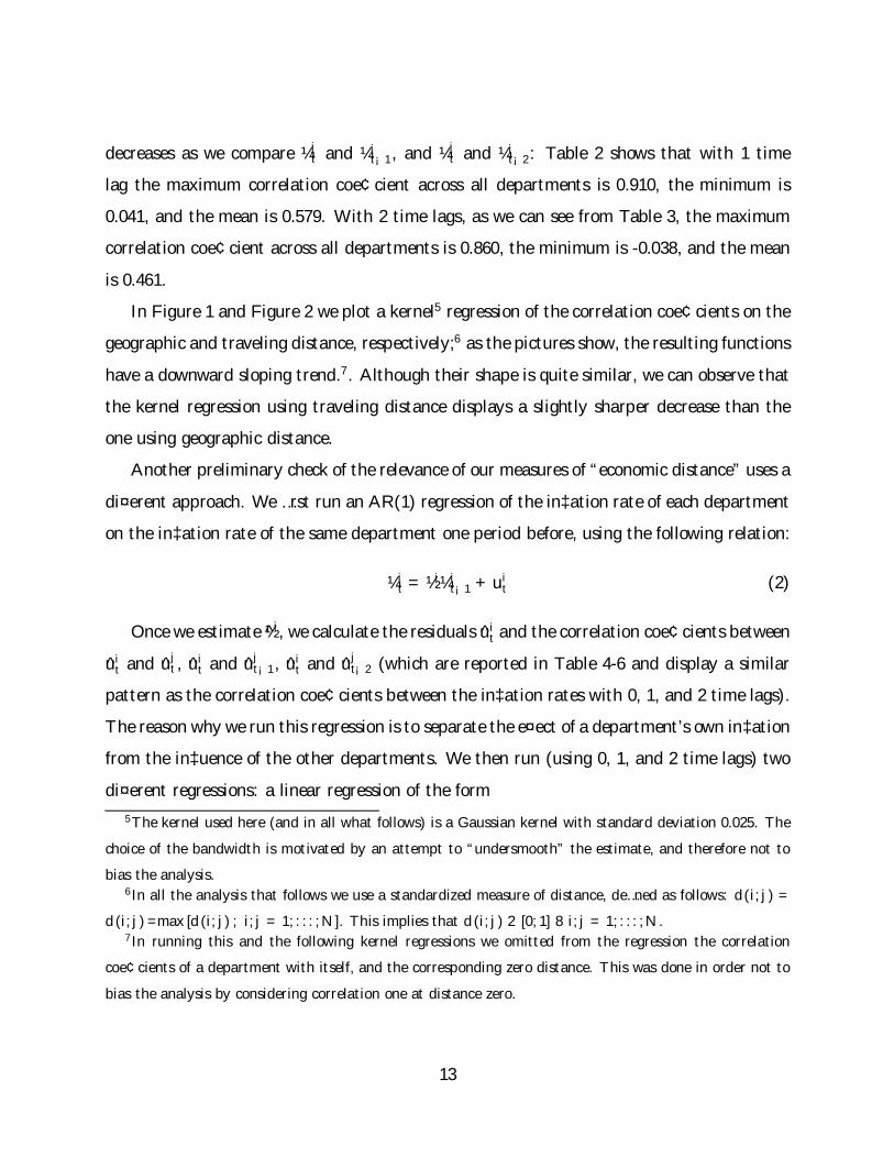
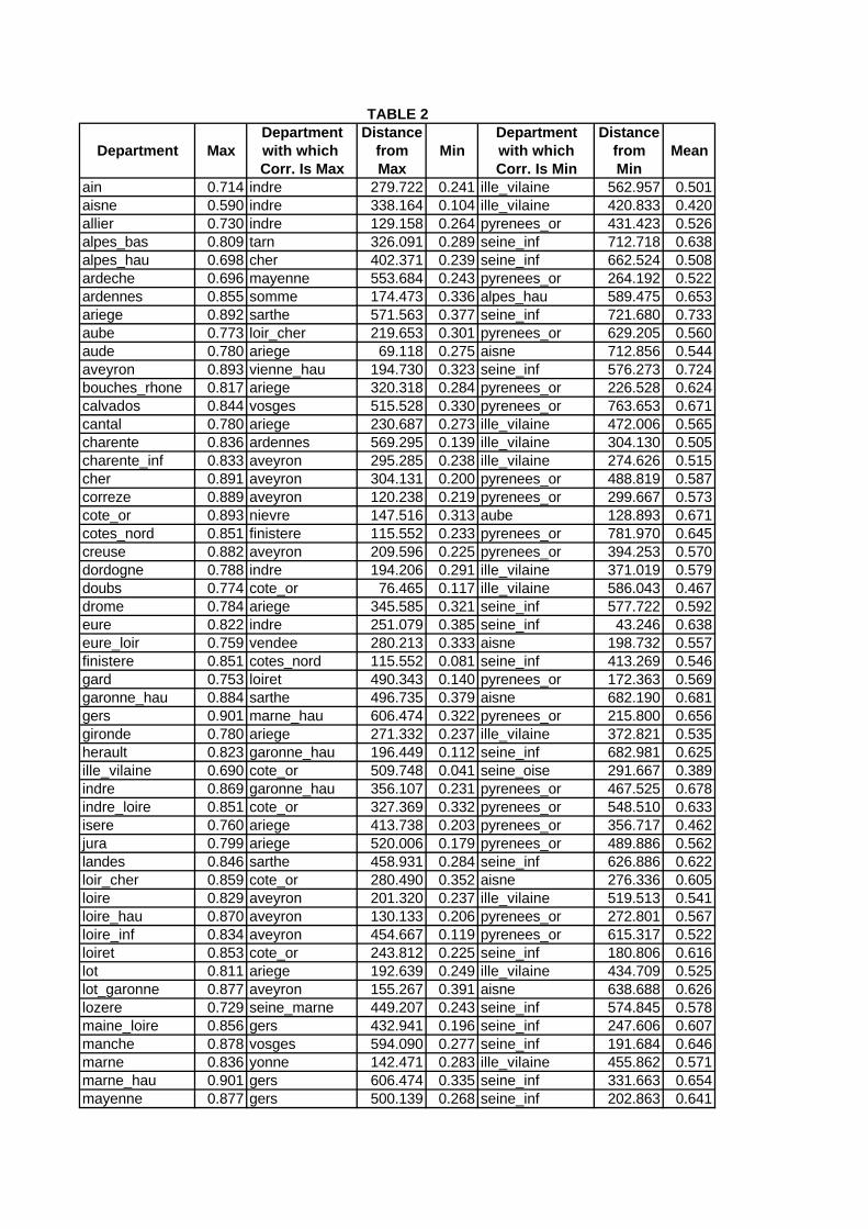
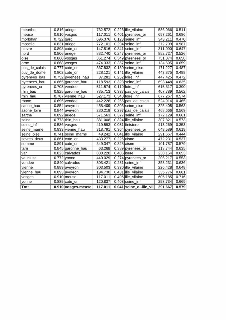
decreases as we compare ¼jt and ¼it¡1, and ¼jt and ¼it¡2: Table 2 shows that with 1 time

lag the maximum correlation coe¢cient across all departments is 0.910, the minimum is

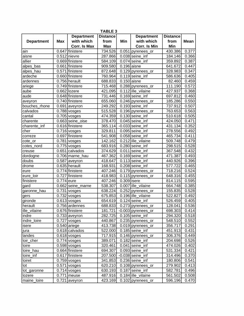
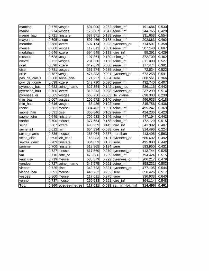
0.041, and the mean is 0.579. With 2 time lags, as we can see from Table 3, the maximum

correlation coe¢cient across all departments is 0.860, the minimum is -0.038, and the mean

is 0.461.

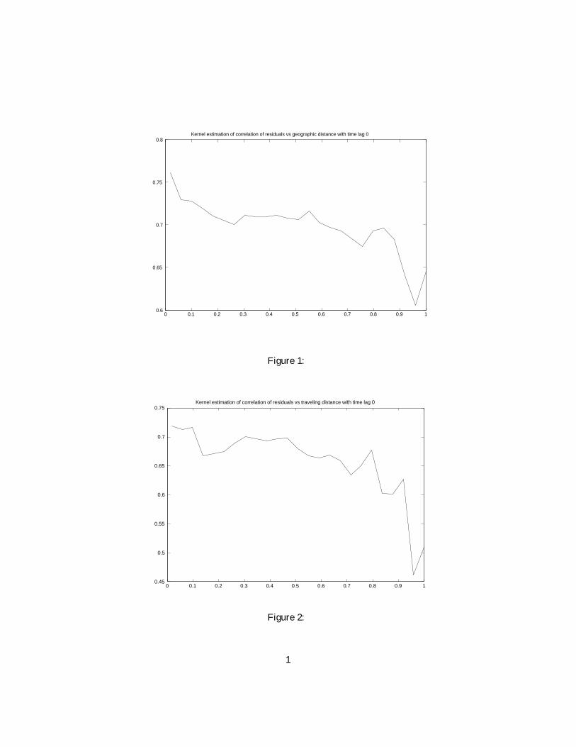
In Figure 1 and Figure 2 we plot a kernel5 regression of the correlation coe¢cients on the

geographic and traveling distance, respectively;6 as the pictures show, the resulting functions

have a downward sloping trend.7. Although their shape is quite similar, we can observe that

the kernel regression using traveling distance displays a slightly sharper decrease than the

one using geographic distance.

Another preliminary check of the relevance of our measures of “economic distance” uses a

di¤erent approach. We …rst run an AR(1) regression of the in‡ation rate of each department

on the in‡ation rate of the same department one period before, using the following relation:

¼it = ½i¼it¡1 + u

it (2)

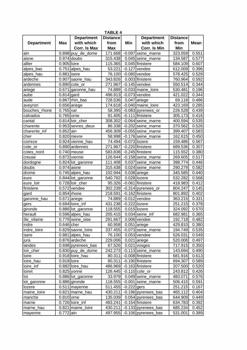
Once we estimate ½i, we calculate the residuals uit and the correlation coe¢cients between

uit and ujt , uit and ujt¡1, uit and ujt¡2 (which are reported in Table 4-6 and display a similar

pattern as the correlation coe¢cients between the in‡ation rates with 0, 1, and 2 time lags).

The reason why we run this regression is to separate the e¤ect of a department’s own in‡ation

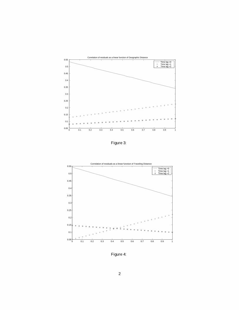
from the in‡uence of the other departments. We then run (using 0, 1, and 2 time lags) two

di¤erent regressions: a linear regression of the form

5The kernel used here (and in all what follows) is a Gaussian kernel with standard deviation 0.025. The

choice of the bandwidth is motivated by an attempt to “undersmooth” the estimate, and therefore not to

bias the analysis.6In all the analysis that follows we use a standardized measure of distance, de…ned as follows: d (i; j) =

d (i; j) = max [d (i; j) ; i; j = 1; : : : ;N ]. This implies that d (i; j) 2 [0; 1] 8 i; j = 1; : : : ;N .7In running this and the following kernel regressions we omitted from the regression the correlation

coe¢cients of a department with itself, and the corresponding zero distance. This was done in order not to

bias the analysis by considering correlation one at distance zero.

13

corr³uit; u

jt

´= ° + ´d (i; j) + »t (3)

where d (i; j) represents the distance between department i and j, i; j = 1; : : : ; 84, and

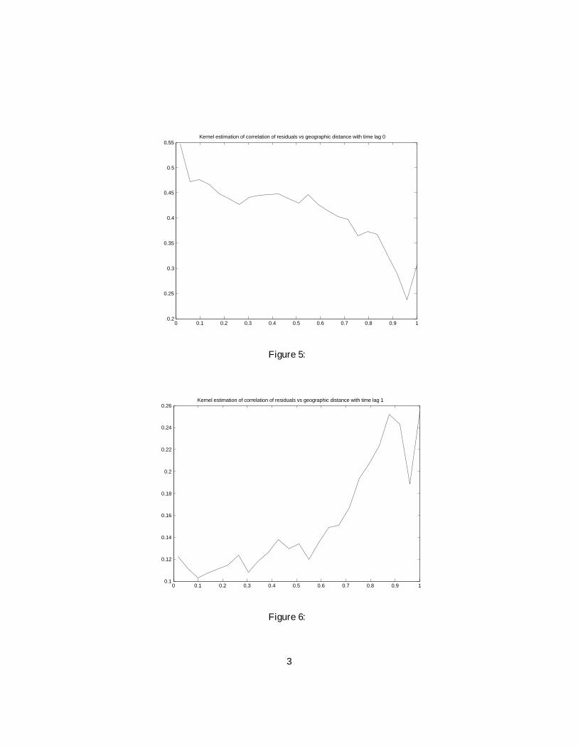
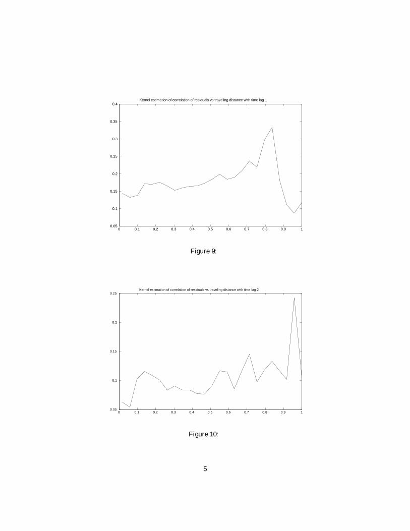
a kernel regression of the residuals on the distance. The estimated coe¢cients of equation

(3) are reported in Table 7 (along with their 95% con…dence interval), while graphs for the

regressions are shown, respectively, in Figures 3-10. As we can see, with no time lag there is

a signi…cant negative relation between correlation of residuals and economic distance; adding

time lags this relation moves to the positive region, but it is much weaker. This trend is

robust to the use of the kernel regression instead of the linear speci…cation.

Thus, the results of this analysis support the conjecture that economic distance plays

an important role in explaining the correlation between in‡ation rates. To study this inter-

dependence and correlation patterns we employ spatial econometrics tools.

4.2 Spatial VAR: Model and Results

We use a model (similar to the one in Chen and Conley [6]) that characterizes the relationship

between departments’ in‡ation rates by the economic distance between them. As already

mentioned, we use as a proxy for economic distance the geographic and the traveling distance;

the basic idea is that if there are two groups of departments with the same position relative

to each other, then there is a replication in the cross section component of our panel data

that can be exploited in order to infer the relationship between the departments.

We denote by ¦t =³¼1t ; ¼

2t ; : : : ; ¼

Nt

´0the vector collecting the in‡ation rates at time

t for the N = 49 departments for which we have a measure of traveling distance8, by

D = (D (1; 2) ; : : : ; D (1; N) ; D (2; 3) ; : : : ; D (2; N) ; : : : ; D (N ¡ 1; N))0 the (geographic or

traveling) distance between departments, by ¹t the growth rate of money, and by IND

8We restrict our attention to these 49 departments in order to be able to compare the results obtained

using geographic distance with those obtained using traveling distance. These departments are evenly spread

across the French territory.

14

the prevailing industry9 in each department; we assume that ¦t evolves according to the

following basic nonlinear VAR model:

¦t+1 = A (D) ¦t + "t+1; "t+1 ´ Q (D)Ãt+1 (4)

where Ãt+1 is an IID sequence with EÃt+1 = 0 and EÃt+1Ã0t+1 = IN . The N £N matrix

A (D) is de…ned as follows:

A (D) =

2666666664

®1 g (D (1; 2)) : : : g (D (1; N))

g (D (2; 1)) ®2 : : : g (D (2; N))

: : : : : : : : : : : :

g (D (N; 1)) g (D (N; 2)) : : : ®N

3777777775

(5)

where the coe¢cients ®i, i = 1; :::; N , represent the e¤ect of ¼it¡1 on ¼it, while the o¤

diagonal elements represent the e¤ect of department j’s in‡ation rate on department i’s

next period in‡ation rate as a function of the distance between the two departments.

We consider as well two other speci…cations of this basic model:

¦t+1 = A (D)¦t + ¯i¹t + "t+1; "t+1 ´ Q (D)Ãt+1 (4’)

¦t+1 = A (D)¦t + IND'+ "t+1; "t+1 ´ Q (D)Ãt+1 (4”)

in order to account in the …rst case for the growth rate of money, and in the second case

(by means of dummy variables) for the prevailing industry (IND) in each department.

Finally, we model the conditional covariance matrix of¦t+1, given by§(D) ´ Q (D)Q (D)0

as follows:9The industries are calicoes, ceramics, coal, cotton, metalwork, ports, silk and textiles. The source of our

data is Jones [12].

15

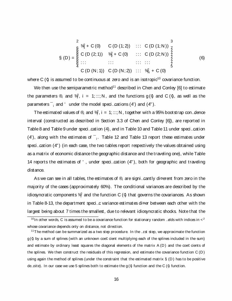
§ (D) =

2666666664

¾21 + C (0) C (D (1; 2)) : : : C (D (1;N ))

C (D (2; 1)) ¾22 + C (0) : : : C (D (2;N ))

: : : : : : : : : : : :

C (D (N; 1)) C (D (N; 2)) : : : ¾2N + C (0)

3777777775

(6)

where C (¢) is assumed to be continuous at zero and is an isotropic10 covariance function.

We then use the semiparametric method11 described in Chen and Conley [6] to estimate

the parameters ®i and ¾2i , i = 1; :::; N , and the functions g (¢) and C (¢), as well as the

parameters ¯i and ' under the model speci…cations (4’) and (4”).

The estimated values of ®i and ¾2i , i = 1; :::; N , together with a 95% bootstrap con…dence

interval (constructed as described in Section 3.3 of Chen and Conley [6]), are reported in

Table 8 and Table 9 under speci…cation (4), and in Table 10 and Table 11 under speci…cation

(4’), along with the estimates of ¯i. Table 12 and Table 13 report these estimates under

speci…cation (4”) (in each case, the two tables report respectively the values obtained using

as a matrix of economic distance the geographic distance and the traveling one), while Table

14 reports the estimates of ', under speci…cation (4”), both for geographic and traveling

distance.

As we can see in all tables, the estimates of ®i are signi…cantly di¤erent from zero in the

majority of the cases (approximately 60%). The conditional variances are described by the

idiosyncratic components ¾2i and the function C (¢) that governs the covariances. As shown

in Table 8-13, the department speci…c variance estimates di¤er between each other with the

largest being about 7 times the smallest, due to relevant idiosyncratic shocks. Note that the

10In other words, C is assumed to be a covariance function for stationary random …elds with indices in <2

whose covariance depends only on distance, not direction.11The method can be summarized as a two step procedure. In the …rst step, we approximate the function

g (¢) by a sum of splines (with an unknown coe¢cient multiplying each of the splines included in the sum)

and estimate by ordinary least squares the diagonal elements of the matrix A (D) and the coe¢cients of

the splines. We then construct the residuals of this regression, and estimate the covariance function C (D)

using again the method of splines (under the constraint that the estimated matrix §(D) has to be positive

de…nite). In our case we use 5 splines both to estimate the g (¢) function and the C (¢) function.

16

estimates of ®i and ¾2i +C (0) obtained by using geographic distance and traveling distance

are very similar, suggesting that these two measures of distance capture similar features of

the economic conditions of the French departments.

At the same time, we can observe that these estimates do not change signi…cantly if we

include in the basic VAR regression the growth rate of money, or a dummy for the prevailing

industry. Looking at Table 10 and Table 11, we can see that it’s not possible to reject the

null hypothesis that ¯i = 0 8 i; although this result is surprising, we believe that the non

signi…cance of the growth rate of money can be explained by the strong multicollinearity of

our time series of money supply with the price levels across departments. Looking at Table

14, we can see as well that we can’t reject the null hypothesis that ' = 0 for all industrial

sectors (even though in this case the non rejection of the null is not as strong as in the case

of the money growth rate). Regarding this result, we believe that it is due to the fact that

the measure we are using is still too inaccurate. In order to get better results we would need

a measure of the amount of production of each single department for each single product,

and of the type of trades between departments.

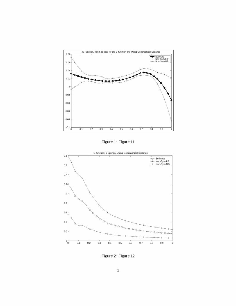
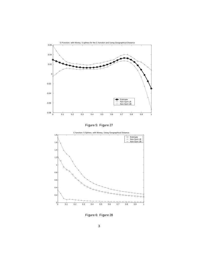
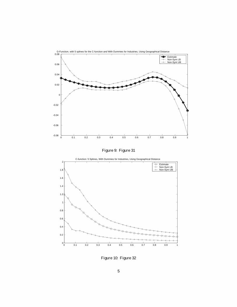
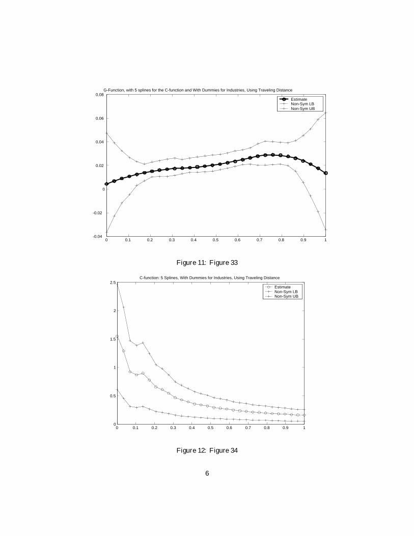
Figure 11 and Figure 12 plot respectively the g (¢) function and the C (¢) function, together

with their 95% bootstrap con…dence interval, obtained by using geographic distance under

speci…cation (4); Figure 13 and Figure 14 plot the same functions and bootstrap con…dence

interval, this time using traveling distance, again under speci…cation (4). The same functions

obtained under speci…cation (4’) and (4”) are plotted, respectively, in Figure 27-34. In all

what follows we will comment Figure 11-14, since, as we can see from the pictures and as

we already discussed, the inclusion of money growth rate or of dummies for the prevailing

industries does not signi…cantly impact our results.

The solid lines with circles in Figure 11 and Figure 13 are our estimates of g (¢) plotted

against the distances in our sample; the solid lines with pluses are the 95% bootstrap con…-

dence intervals (200 draws). The point estimates, both using geographic distance and trav-

eling distance, are relatively small in absolute magnitude (while 1N

Pi ®i is equal to ¡0:211

using geographic distance and ¡0:217 using traveling distance, the maximum value reached

17

by the g function is approximately 0:038 with geographic distance, and 0:025 with traveling

distance), but they are positive and signi…cantly di¤erent from zero.12 Using geographic

distance, the g function is slightly decreasing for distances up to 0:5 (i.e. approximately

the 70th percentile of the non-zero distances), and then it is slightly increasing. Using the

traveling distance we get a g function increasing for almost all distances.

Thus there is evidence of signi…cant (even if maybe small) dynamic spatial correlation

for most distances (both geographic and traveling ones), although the sign is not clear. In

the next Section we will present a series of test to check the robustness of this conclusion.

The solid lines with circles in Figure 12 and Figure 14 are our estimates of C (¢), nor-

malized by the average of the departments variances: 1N

Pi [¾

2i + C (0)]. The solid lines with

pluses are the 95% bootstrap con…dence intervals (200 draws). If all departments variances

were the same, this normalized estimate of C (¢) would be the spatial correlation. Even if,

due to idiosyncratic shocks, this is not the case here, we still get a sense of whether C (¢)is large relative to the departments variances. As we can see from the pictures, using both

measures of economic distance the magnitude of the estimates of C is rather large relative to

the departments variances, even when we consider the lower bound of the con…dence interval.

As we can infer, there is strong evidence that correlation of the shocks in the VAR model

we used is a decreasing function of both geographic and traveling distance. In the next

Section we will present a series of test to check the robustness of this conclusion.

4.3 Robustness of the Results

Given the results we showed in the previous Section, two questions remain opened. The …rst

one regards the problem of whether the g function is in reality a function of the economic

distance, or not simply a constant. The second regards the problem of whether in reality

there is spatial independence across the series, and the results of the previous Section are

12The con…dence intervals do not contain the zero for distances between 0:1 and 0:8, i.e. approximately

between the 5th and the 90th percentile of non-zero geographic distances, and between the 5th and the 95th

percentile of nonzero traveling distances.

18

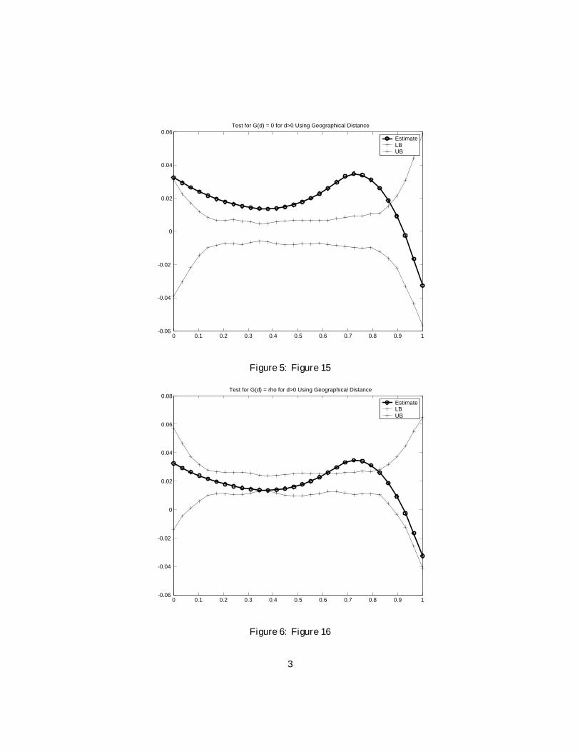
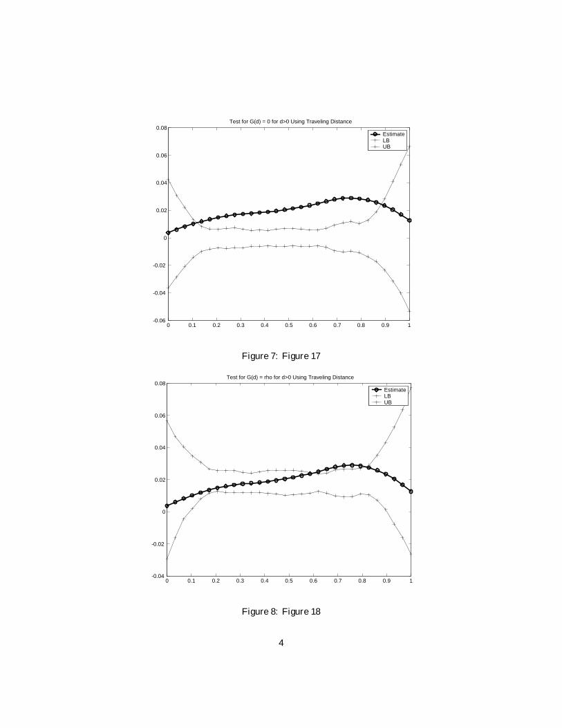
simply driven by the model. In order to answer these questions we run two types of test.

In the …rst one we test, in separate experiments, two null hypotheses:

1. H0 : g (d) = 0 8 d > 0;

2. H0 : g (d) = ± 6= 0 8 d > 0:

In order to test those hypotheses we proceed as follows13. We run a VAR regression similar

to the one in equation (4), in which we specify, respectively, A (D) to be …rst a diagonal

matrix, and then a matrix whose o¤ diagonal elements are all equal to a constant. We then

calculate the residuals under these two speci…cation, and generate bootstrap samples by

drawing independently from the empirical distribution of the residuals and using the VAR

estimates as a data generating model. At this point we use Chen and Conley’s [6] Spatial

VAR method to estimate the g function for each bootstrap sample. We plot in Figure 15-18,

respectively, the results of the two test using …rst geographic and then traveling distance.

As we can see, in both cases we can reject the null hypothesis that g (d) = 0 8 d > 0, but we

can’t reject the null of g being a costant across all distances. This result is consistent with

the conclusions we drew in the previous Section.

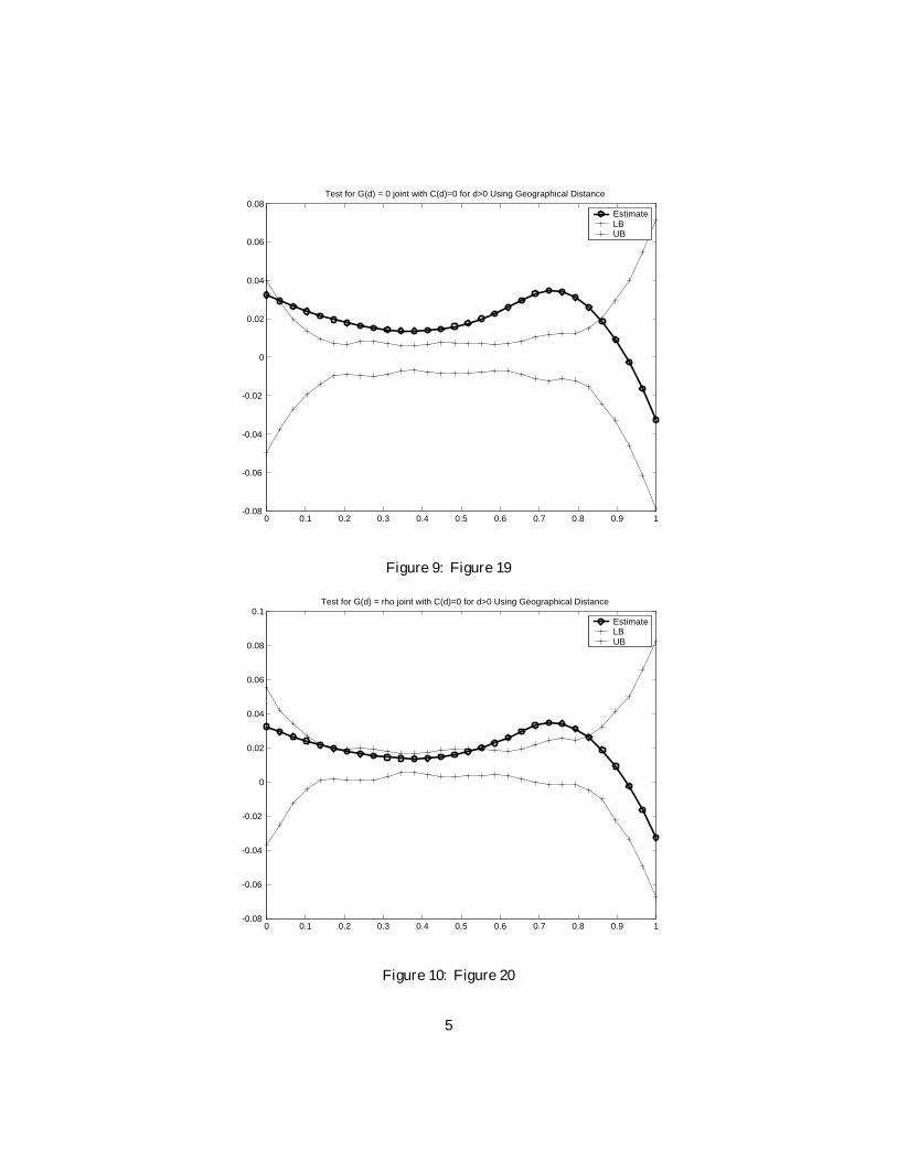
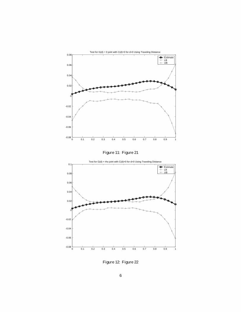
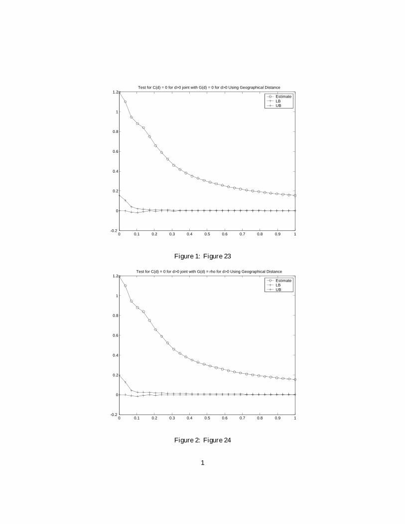
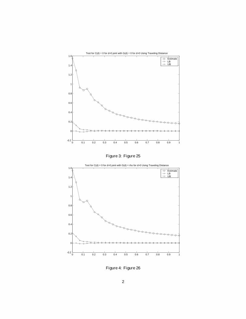
We then test the two following joint hypotheses:

1. H0 : C (d) = 0 and g (d) = 0 8 d > 0;

2. H0 : C (d) = 0 and g (d) = ± 6= 0 8 d > 0:

In words, the …rst null hypothesis is meant to test the complete spatial independence

of our data; the second is meant to test whether there is an e¤ect of other departments

in‡ation rates on the in‡ation rate of a given department, but there is independence in the

VAR shocks.

The procedure adopted to test these hypotheses is similar to the one described above.14

In Figure 19-26 we plot, respectively, the g and the C function with the 95% acceptance13The procedures described here are inspired by the one in Section 3.3 of Chen and Conley [6].14The main di¤erence is in the construction of the bootstrap samples. In order to have independent shocks,

we sample independently from the empirical distribution of shocks for each series separately.

19

region of the null hypotheses, calculated using geographic and traveling distance. As we

can see, we can reject the null of spatial independence. The g function, using both types

of distance, is mainly outside the 95% acceptance region of the null; the C function, again

for both types of distance, is de…nitely far from the 95% acceptance region. Regarding the

second null we are testing, we can again reject the independence of the shocks (again, the

C function is far away from the 95% acceptance region, for both types of distances), but we

can’t reject the hypothesis that the g function is a constant. Therefore also these test are

consistent with the conclusion we reached in the previous Section.

5 Conclusions

During the Revolution France su¤ered a major hyperin‡ation, with the stock of money

growing almost hundred times within …ve years. In an attempt to provide a basis for the

translation of paper money obligations made during this period into metallic equivalents, all

French departments estimated the local value of the Assignats. While in a fully integrated

economy one may expect that the resulting price indices would be very close, if not identical,

between each other, this was not the case in the Revolutionary France: price indices strike

with their wild di¤erences both in levels and growth rates.

Even though some of these di¤erences are undoubtedly due to noise and to non unifor-

mities in the construction of the series, we showed that the rest can be explained by the non

homogeneous level of economic integration among the French departments of the late 17th

century.

The evidence we found is supported by two facts. First, regions which were closer in terms

of geographic or traveling distance had more similar and integrated economies15. Second,

level of depreciation of the Assignats depended also on local economic conditions. (For

15We can support this fact by means of two observations. First, Jones’s [12] data indicates that closer

departments had more common industries than far ones. Second, traveling distance is in a sense endogenous

to the level of economic integration, since departments with more interactions between each other had

probably better communication ways, and in particular better roads.

20

example, authors like Harris [10] and Aftalion [1] claim, areas with worse economic conditions

had higher depreciation of the paper money.)

Using the tools of spatial econometrics to estimate the nonlinear, distance dependent,

VAR model

¦t+1 = A (D) ¦t + "t+1; "t+1 ´ Q (D)Ãt+1 (4)

we did not …nd evidence that the impact of past in‡ation in other departments on current

in‡ation in a particular department depends on our measure of economic distance, although

we found evidence of a signi…cant (even if maybe small) dynamic correlation. But we found

strong evidence that the correlation of the shoks in the VAR model is a decreasing function

of both geographic and traveling distance. A shock to the in‡ation in one department had

higher impact on the in‡ation of close departments than on that of far ones. If these shocks

are attributable to a change in the underlying economic conditions of the departments, we

can conclude that the economic conditions in closer regions were far more important for the

price evolution in a particular department than those in distant regions.

Therefore some of the di¤erences in the value of paper money across departments of the

late 17th century France are attributable to the diverse economic conditions faced by the

di¤erent departments, and to the absence of full economic intergration in the country.

References

[1] Aftalion F., The French Revolution, An Economic Interpretation, Cambridge University

Press.

[2] P. Bairoch, J. Batou and P. Chevre, The Population of the European Cities 800-1850,

Librarie Droz, Geneve 1988,Cambridge (translation).

[3] Bordo M. D.and E. N. White, “A Tale of Two Currencies: British and French Finance

During the Napolenonic Wars”, Journal of Economic History, 1991.

21

[4] Brezis E. S. and F. H. Crouzet, “The Role of Assignats during The French Revolution:

An Evil or A Rescuer?”

[5] Butel P., “Revolution and The Urban Economy: Maritime Cities and Continental

Cities”, in Reshaping The France, Ed’s A. Forrest and P. Jones, Manchester Univer-

sity Press, New York, 1991.

[6] Chen X. and T. G. Conley, “A New Semiparametric Spatial Model for Panel Time

Series”, forthcoming Journal of Econometrics, 2000.

[7] Crouzet F., Britain Ascendant: Comparative Studies in Franco-British Economic His-

tory, Cambridge University Press, Cambridge, 1985.

[8] Crouzet F., Britain, France and International Commerce, VARIORUM, Aldershot,

1996.

[9] Le Go¤ T. F. A., “The Revolution and The Rural Economy”, in Reshaping The France,

Ed’s A. Forrest and P. Jones, Manchester University Press, New York, 1991.

[10] Harris S. E., The Assignats, Harvard University Press, Cambridge, 1930.

[11] Fischer D. H. The Great Wave, Oxford University Press, Oxford, 1996.

[12] Jones C., The Longman Companion to The French Revolution, Longman 1990.

[13] Sargent T. J. and F. R. Velde, “Macroeconomic Features of the French Revolution”,

Journal of Political Economy, 1995.

[14] White E. N., “Was There A Solution to the Ancien Regime’s Financial Dilemma”,

Journal of Economic History, 1989.

[15] White E. N., “The French Revolution and The Politics of Government Finance, 1770-

1815”, Journal of Economic History, 1995.

22

6 Appendix

23

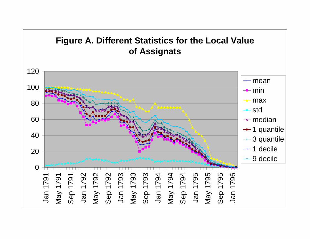
Figure A. Different Statistics for the Local Value of Assignats

0

20

40

60

80

100

120

Jan

1791

May

179

1

Sep

179

1

Jan

1792

May

179

2

Sep

179

2

Jan

1793

May

179

3

Sep

179

3

Jan

1794

May

179

4

Sep

179

4

Jan

1795

May

179

5

Sep

179

5

Jan

1796

meanminmaxstdmedian1 quantile3 quantile1 decile9 decile

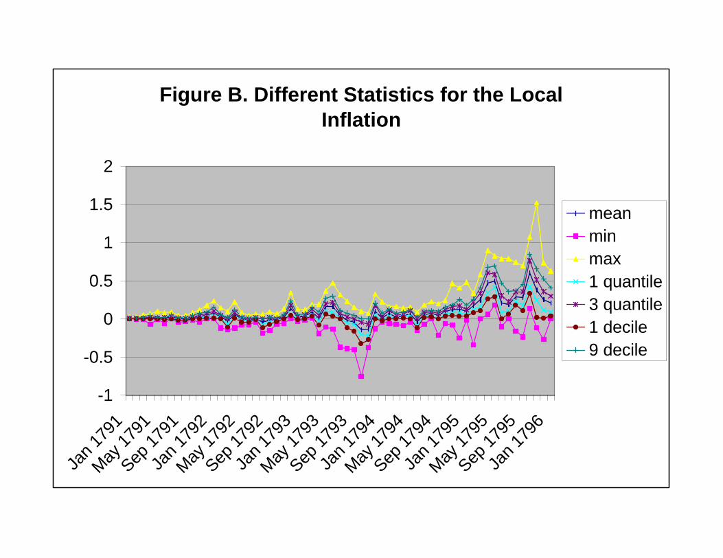
Figure B. Different Statistics for the Local Inflation

-1

-0.5

0

0.5

1

1.5

2

Jan

1791

May

179

1

Sep 1

791

Jan

1792

May

179

2

Sep 1

792

Jan

1793

May

179

3

Sep 1

793

Jan

1794

May

179

4

Sep 1

794

Jan

1795

May

179

5

Sep 1

795

Jan

1796

meanminmax1 quantile3 quantile1 decile9 decile

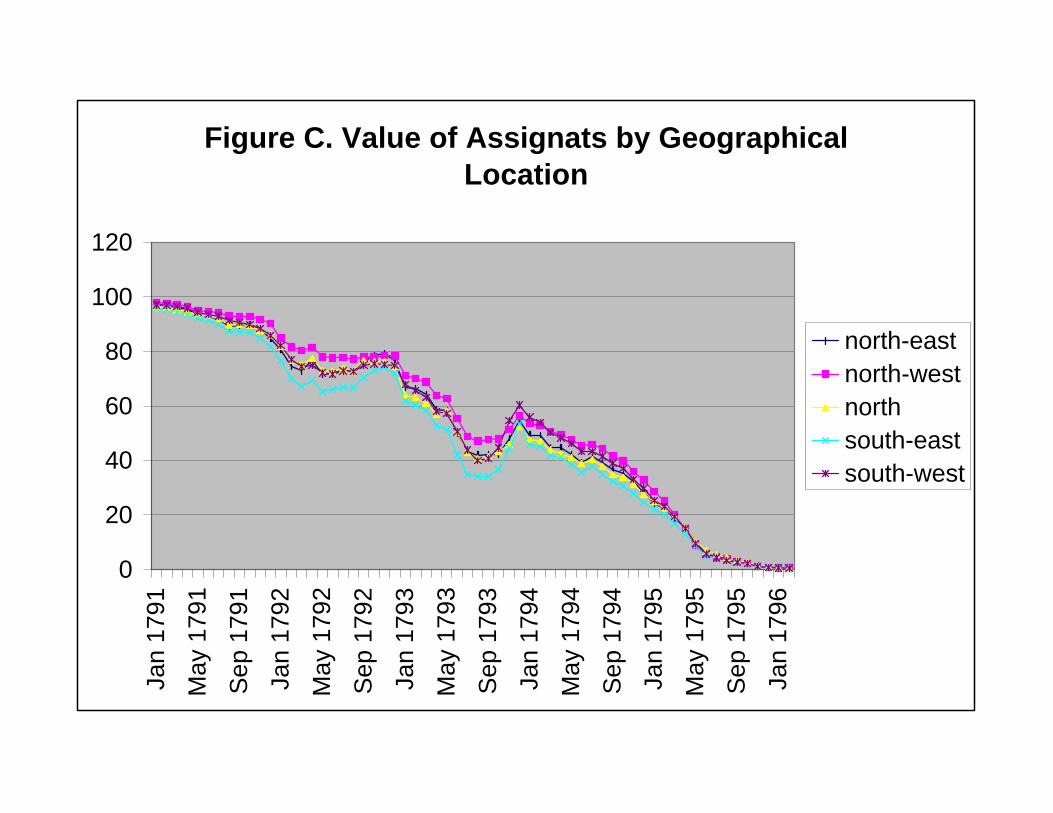
Figure C. Value of Assignats by Geographical Location

0

20

40

60

80

100

120

Jan

1791

May

179

1

Sep

179

1

Jan

1792

May

179

2

Sep

179

2

Jan

1793

May

179

3

Sep

179

3

Jan

1794

May

179

4

Sep

179

4

Jan

1795

May

179

5

Sep

179

5

Jan

1796

north-eastnorth-westnorthsouth-eastsouth-west

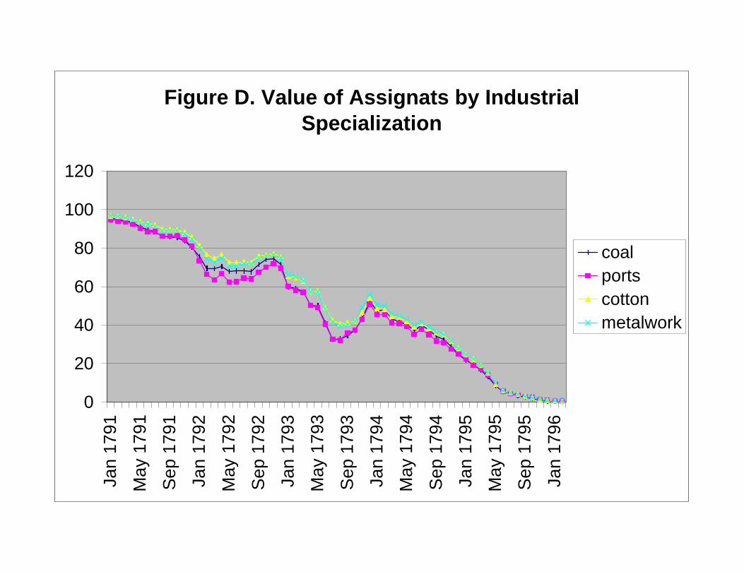
Figure D. Value of Assignats by Industrial Specialization

0

20

40

60

80

100

120

Jan

1791

May

179

1

Sep

179

1

Jan

1792

May

179

2

Sep

179

2

Jan

1793

May

179

3

Sep

179

3

Jan

1794

May

179

4

Sep

179

4

Jan

1795

May

179

5

Sep

179

5

Jan

1796

coalportscottonmetalwork

0 0.1 0.2 0.3 0.4 0.5 0.6 0.7 0.8 0.9 10.6

0.65

0.7

0.75

0.8Kernel estimation of correlation of residuals vs geographic distance with time lag 0

Figure 1:

0 0.1 0.2 0.3 0.4 0.5 0.6 0.7 0.8 0.9 10.45

0.5

0.55

0.6

0.65

0.7

0.75Kernel estimation of correlation of residuals vs traveling distance with time lag 0

Figure 2:

1

0 0.1 0.2 0.3 0.4 0.5 0.6 0.7 0.8 0.9 10.05

0.1

0.15

0.2

0.25

0.3

0.35

0.4

0.45

0.5

0.55Correlation of residuals as a linear function of Geographic Distance

Time lag =0Time lag =1Time lag =2

Figure 3:

0 0.1 0.2 0.3 0.4 0.5 0.6 0.7 0.8 0.9 10.05

0.1

0.15

0.2

0.25

0.3

0.35

0.4

0.45

0.5

0.55Correlation of residuals as a linear function of Traveling Distance

Time lag =0Time lag =1Time lag =2

Figure 4:

2

0 0.1 0.2 0.3 0.4 0.5 0.6 0.7 0.8 0.9 10.2

0.25

0.3

0.35

0.4

0.45

0.5

0.55Kernel estimation of correlation of residuals vs geographic distance with time lag 0

Figure 5:

0 0.1 0.2 0.3 0.4 0.5 0.6 0.7 0.8 0.9 10.1

0.12

0.14

0.16

0.18

0.2

0.22

0.24

0.26Kernel estimation of correlation of residuals vs geographic distance with time lag 1

Figure 6:

3

0 0.1 0.2 0.3 0.4 0.5 0.6 0.7 0.8 0.9 10.02

0.04

0.06

0.08

0.1

0.12

0.14

0.16

0.18Kernel estimation of correlation of residuals vs geographic distance with time lag 2

Figure 7:

0 0.1 0.2 0.3 0.4 0.5 0.6 0.7 0.8 0.9 10.15

0.2

0.25

0.3

0.35

0.4

0.45

0.5

0.55Kernel estimation of correlation of residuals vs traveling distance with time lag 0

Figure 8:

4

0 0.1 0.2 0.3 0.4 0.5 0.6 0.7 0.8 0.9 10.05

0.1

0.15

0.2

0.25

0.3

0.35

0.4Kernel estimation of correlation of residuals vs traveling distance with time lag 1

Figure 9:

0 0.1 0.2 0.3 0.4 0.5 0.6 0.7 0.8 0.9 10.05

0.1

0.15

0.2

0.25Kernel estimation of correlation of residuals vs traveling distance with time lag 2

Figure 10:

5

0 0.1 0.2 0.3 0.4 0.5 0.6 0.7 0.8 0.9 1-0.1

-0.08

-0.06

-0.04

-0.02

0

0.02

0.04

0.06

0.08G-Function, with 5 splines for the C-function and Using Geographical Distance

Estimate Non-Sym LBNon-Sym UB

Figure 1: Figure 11

0 0.1 0.2 0.3 0.4 0.5 0.6 0.7 0.8 0.9 10

0.2

0.4

0.6

0.8

1

1.2

1.4

1.6

1.8C-function: 5 Splines, Using Geographical Distance

Estimate Non-Sym LBNon-Sym UB

Figure 2: Figure 12

1

0 0.1 0.2 0.3 0.4 0.5 0.6 0.7 0.8 0.9 1-0.04

-0.02

0

0.02

0.04

0.06

0.08G-Function, with 5 splines for the C-function and Using Traveling Distance

Estimate Non-Sym LBNon-Sym UB

Figure 3: Figure 13

0 0.1 0.2 0.3 0.4 0.5 0.6 0.7 0.8 0.9 10

0.5

1

1.5

2

2.5C-function: 5 Splines, Using Traveling Distance

Estimate Non-Sym LBNon-Sym UB

Figure 4: Figure 14

2

0 0.1 0.2 0.3 0.4 0.5 0.6 0.7 0.8 0.9 1-0.06

-0.04

-0.02

0

0.02

0.04

0.06Test for G(d) = 0 for d>0 Using Geographical Distance

EstimateLB UB

Figure 5: Figure 15

0 0.1 0.2 0.3 0.4 0.5 0.6 0.7 0.8 0.9 1-0.06

-0.04

-0.02

0

0.02

0.04

0.06

0.08Test for G(d) = rho for d>0 Using Geographical Distance

EstimateLB UB

Figure 6: Figure 16

3

0 0.1 0.2 0.3 0.4 0.5 0.6 0.7 0.8 0.9 1-0.06

-0.04

-0.02

0

0.02

0.04

0.06

0.08Test for G(d) = 0 for d>0 Using Traveling Distance

EstimateLB UB

Figure 7: Figure 17

0 0.1 0.2 0.3 0.4 0.5 0.6 0.7 0.8 0.9 1-0.04

-0.02

0

0.02

0.04

0.06

0.08Test for G(d) = rho for d>0 Using Traveling Distance

EstimateLB UB

Figure 8: Figure 18

4

0 0.1 0.2 0.3 0.4 0.5 0.6 0.7 0.8 0.9 1-0.08

-0.06

-0.04

-0.02

0

0.02

0.04

0.06

0.08Test for G(d) = 0 joint with C(d)=0 for d>0 Using Geographical Distance

EstimateLB UB

Figure 9: Figure 19

0 0.1 0.2 0.3 0.4 0.5 0.6 0.7 0.8 0.9 1-0.08

-0.06

-0.04

-0.02

0

0.02

0.04

0.06

0.08

0.1Test for G(d) = rho joint with C(d)=0 for d>0 Using Geographical Distance

EstimateLB UB

Figure 10: Figure 20

5

0 0.1 0.2 0.3 0.4 0.5 0.6 0.7 0.8 0.9 1-0.08

-0.06

-0.04

-0.02

0

0.02

0.04

0.06

0.08Test for G(d) = 0 joint with C(d)=0 for d>0 Using Traveling Distance

EstimateLB UB

Figure 11: Figure 21

0 0.1 0.2 0.3 0.4 0.5 0.6 0.7 0.8 0.9 1-0.08

-0.06

-0.04

-0.02

0

0.02

0.04

0.06

0.08

0.1Test for G(d) = rho joint with C(d)=0 for d>0 Using Traveling Distance

EstimateLB UB

Figure 12: Figure 22

6

0 0.1 0.2 0.3 0.4 0.5 0.6 0.7 0.8 0.9 1-0.2

0

0.2

0.4

0.6

0.8

1

1.2Test for C(d) = 0 for d>0 joint with G(d) = 0 for d>0 Using Geographical Distance

EstimateLB UB

Figure 1: Figure 23

0 0.1 0.2 0.3 0.4 0.5 0.6 0.7 0.8 0.9 1-0.2

0

0.2

0.4

0.6

0.8

1

1.2Test for C(d) = 0 for d>0 joint with G(d) = rho for d>0 Using Geographical Distance

EstimateLB UB

Figure 2: Figure 24

1

0 0.1 0.2 0.3 0.4 0.5 0.6 0.7 0.8 0.9 1-0.2

0

0.2

0.4

0.6

0.8

1

1.2

1.4

1.6Test for C(d) = 0 for d>0 joint with G(d) = 0 for d>0 Using Traveling Distance

EstimateLB UB

Figure 3: Figure 25

0 0.1 0.2 0.3 0.4 0.5 0.6 0.7 0.8 0.9 1-0.2

0

0.2

0.4

0.6

0.8

1

1.2

1.4

1.6Test for C(d) = 0 for d>0 joint with G(d) = rho for d>0 Using Traveling Distance

EstimateLB UB

Figure 4: Figure 26

2

0 0.1 0.2 0.3 0.4 0.5 0.6 0.7 0.8 0.9 1-0.08

-0.06

-0.04

-0.02

0

0.02

0.04

0.06G-Function, with Money, 5 splines for the C-function and Using Geographical Distance

Estimate Non-Sym LBNon-Sym UB

Figure 5: Figure 27

0 0.1 0.2 0.3 0.4 0.5 0.6 0.7 0.8 0.9 10

0.2

0.4

0.6

0.8

1

1.2

1.4

1.6

1.8C-function: 5 Splines, with Money, Using Geographical Distance

Estimate Non-Sym LBNon-Sym UB

Figure 6: Figure 28

3

0 0.1 0.2 0.3 0.4 0.5 0.6 0.7 0.8 0.9 1-0.04

-0.02

0

0.02

0.04

0.06

0.08G-Function, with Money, 5 splines for the C-function and Using Traveling Distance

Estimate Non-Sym LBNon-Sym UB

Figure 7: Figure 29

0 0.1 0.2 0.3 0.4 0.5 0.6 0.7 0.8 0.9 1-1.5

-1

-0.5

0

0.5

1

1.5

2

2.5C-function: 5 Splines, with Money, Using Traveling Distance

Estimate Non-Sym LBNon-Sym UB

Figure 8: Figure 30

4

0 0.1 0.2 0.3 0.4 0.5 0.6 0.7 0.8 0.9 1-0.08

-0.06

-0.04

-0.02

0

0.02

0.04

0.06

0.08G-Function, with 5 splines for the C-function and With Dummies for Industries, Using Geographical Distance

Estimate Non-Sym LBNon-Sym UB

Figure 9: Figure 31

0 0.1 0.2 0.3 0.4 0.5 0.6 0.7 0.8 0.9 10

0.2

0.4

0.6

0.8

1

1.2

1.4

1.6

1.8

2C-function: 5 Splines, With Dummies for Industries, Using Geographical Distance

Estimate Non-Sym LBNon-Sym UB

Figure 10: Figure 32

5

0 0.1 0.2 0.3 0.4 0.5 0.6 0.7 0.8 0.9 1-0.04

-0.02

0

0.02

0.04

0.06

0.08G-Function, with 5 splines for the C-function and With Dummies for Industries, Using Traveling Distance

Estimate Non-Sym LBNon-Sym UB

Figure 11: Figure 33

0 0.1 0.2 0.3 0.4 0.5 0.6 0.7 0.8 0.9 10

0.5

1

1.5

2

2.5C-function: 5 Splines, With Dummies for Industries, Using Traveling Distance

Estimate Non-Sym LBNon-Sym UB

Figure 12: Figure 34

6

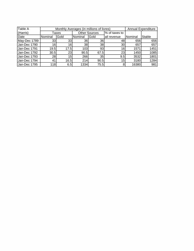
Table A(Harris) % of taxes to Date Nominal Gold Nominal Gold all revenue Nominal StableMay-Dec 1789 33 33 36 36 48 656 656Jan-Dec 1790 16 16 38 38 30 657 657Jan-Dec 1791 19.5 17.5 103 93 16 1571 1451Jan-Dec 1792 30.5 23 90.5 67.5 23 1450 1085Jan-Dec 1793 28 15 266 35 9.5 3532 1801Jan-Dec 1794 41 16.5 214 90.5 15 3180 1284Jan-Dec 1795 118 6.5 1334 75.5 8 16380 981

Annual ExpenditureMonthly Averages (in millions of livres)Taxes Other Sources

Table B The Issue of Assignat during the French Revolution(Brezis-Crouzet) (million of livres)Year Month Decreed Issued Burned In Smallest

Circulation Denom.1789 19-Dec 400 1000

1790 17-Apr 20029-Sep 800

8-Oct 5031-Dec 590 590

1791 6-May 55-Jun 600 1150 170 980

17-Dec 30031-Dec 1730 370 1360 0.5

1792 27-Apr 300 2075 475 160031-May 2200 1650

31-Jul 30024-Oct 40031-Dec 2870 650 2220

1793 1-Feb 800 3100 700 24007-May 1200

31-Aug 4800 950 385028-Sep 2000

1794 19-Jun 1205 8236 2182 605422-Sep 8932 2358 6574

1795 21-Mar 10787 2639 814823-Sep 20394 3123 17271

1796 9-Feb 40279 5775 34504

Department Distance Department DistanceDepartment Max with which from Min with which from Mean

Corr. Is Max Max Corr. Is Min Minain 0.929 allier 150.620 0.347 pyrenees_bas 546.925 0.754aisne 0.977 doubs 315.438 0.319 pyrenees_or 765.626 0.719allier 0.938 loire 115.365 0.438 seine_inf 359.892 0.796alpes_bas 0.857 alpes_hau 53.221 0.362 seine_inf 712.718 0.687alpes_hau 0.887 isere 76.100 0.373 seine_inf 662.524 0.718ardeche 0.940 saone_hau 343.826 0.464 seine_inf 586.636 0.788ardennes 0.934 cote_or 271.967 0.394 seine_inf 265.296 0.676ariege 0.895 garonne_hau 74.889 0.392 seine_inf 721.680 0.644aube 0.837 gard 496.913 0.278 seine_inf 253.604 0.620aude 0.913 rhin_bas 728.536 0.374 pyrenees_or 72.888 0.719aveyron 0.875 ariege 174.618 0.410 seine_inf 576.273 0.672bouches_rhone 0.939 var 58.395 0.414 pyrenees_or 226.528 0.775calvados 0.960 orne 91.405 0.406 seine_inf 109.045 0.760cantal 0.912 loir_cher 308.302 0.472 seine_inf 510.618 0.779charente 0.957 sevres_deux 86.338 0.322 pyrenees_or 395.760 0.739charente_inf 0.916 allier 320.191 0.414 lozere 351.376 0.761cher 0.940 nievre 58.998 0.420 seine_inf 278.556 0.758correze 0.963 vienne_hau 74.494 0.415 seine_inf 465.734 0.793cote_or 0.934 ardennes 271.967 0.300 seine_inf 374.256 0.669cotes_nord 0.893 meuse 583.838 0.489 finistere 115.552 0.726creuse 0.938 vienne 126.644 0.417 seine_inf 367.548 0.766dordogne 0.909 lot_garonne 111.408 0.418 seine_inf 471.387 0.717doubs 0.977 aisne 315.438 0.314 pyrenees_or 561.048 0.741drome 0.861 nord 619.634 0.382 pyrenees_or 295.719 0.725eure 0.939 lot_garonne 540.782 0.449 seine_inf 43.246 0.809eure_loir 0.879 loir_cher 95.326 0.350 seine_inf 113.532 0.679finistere 0.741 vendee 302.239 0.035 pyrenees_or 804.247 0.541gard 0.892 rhone 218.591 0.310 finistere 801.892 0.674garonne_hau 0.895 ariege 74.889 0.400 seine_inf 647.158 0.706gers 0.859 vienne_hau 245.847 0.422 lozere 251.215 0.716gironde 0.932 lot_garonne 118.555 0.384 lozere 324.092 0.764herault 0.855 orne 610.787 0.396 seine_inf 682.981 0.723ille_vilaine 0.822 cantal 472.006 0.274 seine_inf 250.696 0.613indre 0.910 vienne_hau 114.324 0.499 pyrenees_or 467.525 0.774indre_loire 0.926 orne 123.838 0.477 seine_inf 229.715 0.800isere 0.908 meurthe 392.674 0.336 seine_inf 587.995 0.696jura 0.940 ardeche 229.006 0.412 seine_inf 451.913 0.745landes 0.870 rhin_hau 764.913 0.351 seine_inf 626.886 0.703loir_cher 0.946 orne 130.192 0.503 vaucluse 488.565 0.763loire 0.948 loire_hau 80.311 0.423 lozere 144.796 0.791loire_hau 0.948 loire 80.311 0.373 finistere 694.307 0.791loire_inf 0.915 loire_hau 486.969 0.280 lozere 495.575 0.719loiret 0.920 manche 280.911 0.491 pyrenees_or 583.200 0.740lot 0.925 meurthe 644.959 0.393 pyrenees_or 279.902 0.766lot_garonne 0.939 eure 540.782 0.450 seine_inf 582.781 0.822lozere 0.734 meuse 487.916 0.280 loire_inf 495.575 0.524maine_loire 0.923 marne_hau 430.211 0.318 pyrenees_bas 465.112 0.716manche 0.920 loiret 280.911 0.437 seine_inf 191.684 0.751marne 0.883 cote_or 188.620 0.424 lozere 497.629 0.687marne_hau 0.923 maine_loire 430.211 0.453 pyrenees_bas 685.234 0.772mayenne 0.901 ain 497.955 0.351 pyrenees_or 661.550 0.739

TABLE 1

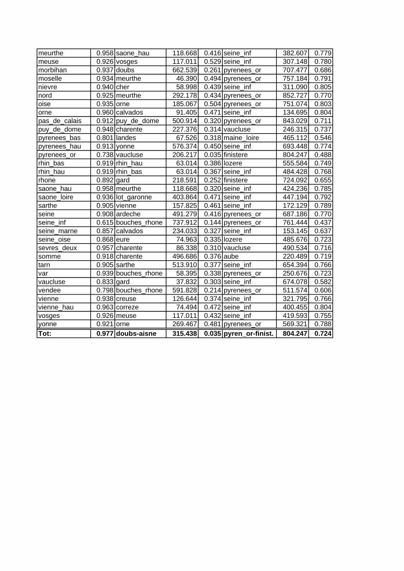
meurthe 0.958 saone_hau 118.668 0.416 seine_inf 382.607 0.779meuse 0.926 vosges 117.011 0.529 seine_inf 307.148 0.780morbihan 0.937 doubs 662.539 0.261 pyrenees_or 707.477 0.686moselle 0.934 meurthe 46.390 0.494 pyrenees_or 757.184 0.791nievre 0.940 cher 58.998 0.439 seine_inf 311.090 0.805nord 0.925 meurthe 292.178 0.434 pyrenees_or 852.727 0.770oise 0.935 orne 185.067 0.504 pyrenees_or 751.074 0.803orne 0.960 calvados 91.405 0.471 seine_inf 134.695 0.804pas_de_calais 0.912 puy_de_dome 500.914 0.320 pyrenees_or 843.029 0.711puy_de_dome 0.948 charente 227.376 0.314 vaucluse 246.315 0.737pyrenees_bas 0.801 landes 67.526 0.318 maine_loire 465.112 0.546pyrenees_hau 0.913 yonne 576.374 0.450 seine_inf 693.448 0.774pyrenees_or 0.738 vaucluse 206.217 0.035 finistere 804.247 0.488rhin_bas 0.919 rhin_hau 63.014 0.386 lozere 555.584 0.749rhin_hau 0.919 rhin_bas 63.014 0.367 seine_inf 484.428 0.768rhone 0.892 gard 218.591 0.252 finistere 724.092 0.655saone_hau 0.958 meurthe 118.668 0.320 seine_inf 424.236 0.785saone_loire 0.936 lot_garonne 403.864 0.471 seine_inf 447.194 0.792sarthe 0.905 vienne 157.825 0.461 seine_inf 172.129 0.789seine 0.908 ardeche 491.279 0.416 pyrenees_or 687.186 0.770seine_inf 0.615 bouches_rhone 737.912 0.144 pyrenees_or 761.444 0.437seine_marne 0.857 calvados 234.033 0.327 seine_inf 153.145 0.637seine_oise 0.868 eure 74.963 0.335 lozere 485.676 0.723sevres_deux 0.957 charente 86.338 0.310 vaucluse 490.534 0.716somme 0.918 charente 496.686 0.376 aube 220.489 0.719tarn 0.905 sarthe 513.910 0.377 seine_inf 654.394 0.766var 0.939 bouches_rhone 58.395 0.338 pyrenees_or 250.676 0.723vaucluse 0.833 gard 37.832 0.303 seine_inf 674.078 0.582vendee 0.798 bouches_rhone 591.828 0.214 pyrenees_or 511.574 0.606vienne 0.938 creuse 126.644 0.374 seine_inf 321.795 0.766vienne_hau 0.963 correze 74.494 0.472 seine_inf 400.455 0.804vosges 0.926 meuse 117.011 0.432 seine_inf 419.593 0.755yonne 0.921 orne 269.467 0.481 pyrenees_or 569.321 0.788Tot: 0.977 doubs-aisne 315.438 0.035 pyren_or-finist. 804.247 0.724

Department Distance Department DistanceDepartment Max with which from Min with which from Mean

Corr. Is Max Max Corr. Is Min Minain 0.714 indre 279.722 0.241 ille_vilaine 562.957 0.501aisne 0.590 indre 338.164 0.104 ille_vilaine 420.833 0.420allier 0.730 indre 129.158 0.264 pyrenees_or 431.423 0.526alpes_bas 0.809 tarn 326.091 0.289 seine_inf 712.718 0.638alpes_hau 0.698 cher 402.371 0.239 seine_inf 662.524 0.508ardeche 0.696 mayenne 553.684 0.243 pyrenees_or 264.192 0.522ardennes 0.855 somme 174.473 0.336 alpes_hau 589.475 0.653ariege 0.892 sarthe 571.563 0.377 seine_inf 721.680 0.733aube 0.773 loir_cher 219.653 0.301 pyrenees_or 629.205 0.560aude 0.780 ariege 69.118 0.275 aisne 712.856 0.544aveyron 0.893 vienne_hau 194.730 0.323 seine_inf 576.273 0.724bouches_rhone 0.817 ariege 320.318 0.284 pyrenees_or 226.528 0.624calvados 0.844 vosges 515.528 0.330 pyrenees_or 763.653 0.671cantal 0.780 ariege 230.687 0.273 ille_vilaine 472.006 0.565charente 0.836 ardennes 569.295 0.139 ille_vilaine 304.130 0.505charente_inf 0.833 aveyron 295.285 0.238 ille_vilaine 274.626 0.515cher 0.891 aveyron 304.131 0.200 pyrenees_or 488.819 0.587correze 0.889 aveyron 120.238 0.219 pyrenees_or 299.667 0.573cote_or 0.893 nievre 147.516 0.313 aube 128.893 0.671cotes_nord 0.851 finistere 115.552 0.233 pyrenees_or 781.970 0.645creuse 0.882 aveyron 209.596 0.225 pyrenees_or 394.253 0.570dordogne 0.788 indre 194.206 0.291 ille_vilaine 371.019 0.579doubs 0.774 cote_or 76.465 0.117 ille_vilaine 586.043 0.467drome 0.784 ariege 345.585 0.321 seine_inf 577.722 0.592eure 0.822 indre 251.079 0.385 seine_inf 43.246 0.638eure_loir 0.759 vendee 280.213 0.333 aisne 198.732 0.557finistere 0.851 cotes_nord 115.552 0.081 seine_inf 413.269 0.546gard 0.753 loiret 490.343 0.140 pyrenees_or 172.363 0.569garonne_hau 0.884 sarthe 496.735 0.379 aisne 682.190 0.681gers 0.901 marne_hau 606.474 0.322 pyrenees_or 215.800 0.656gironde 0.780 ariege 271.332 0.237 ille_vilaine 372.821 0.535herault 0.823 garonne_hau 196.449 0.112 seine_inf 682.981 0.625ille_vilaine 0.690 cote_or 509.748 0.041 seine_oise 291.667 0.389indre 0.869 garonne_hau 356.107 0.231 pyrenees_or 467.525 0.678indre_loire 0.851 cote_or 327.369 0.332 pyrenees_or 548.510 0.633isere 0.760 ariege 413.738 0.203 pyrenees_or 356.717 0.462jura 0.799 ariege 520.006 0.179 pyrenees_or 489.886 0.562landes 0.846 sarthe 458.931 0.284 seine_inf 626.886 0.622loir_cher 0.859 cote_or 280.490 0.352 aisne 276.336 0.605loire 0.829 aveyron 201.320 0.237 ille_vilaine 519.513 0.541loire_hau 0.870 aveyron 130.133 0.206 pyrenees_or 272.801 0.567loire_inf 0.834 aveyron 454.667 0.119 pyrenees_or 615.317 0.522loiret 0.853 cote_or 243.812 0.225 seine_inf 180.806 0.616lot 0.811 ariege 192.639 0.249 ille_vilaine 434.709 0.525lot_garonne 0.877 aveyron 155.267 0.391 aisne 638.688 0.626lozere 0.729 seine_marne 449.207 0.243 seine_inf 574.845 0.578maine_loire 0.856 gers 432.941 0.196 seine_inf 247.606 0.607manche 0.878 vosges 594.090 0.277 seine_inf 191.684 0.646marne 0.836 yonne 142.471 0.283 ille_vilaine 455.862 0.571marne_hau 0.901 gers 606.474 0.335 seine_inf 331.663 0.654mayenne 0.877 gers 500.139 0.268 seine_inf 202.863 0.641

TABLE 2

meurthe 0.816 ariege 732.572 0.223 ille_vilaine 586.066 0.511meuse 0.910 vosges 117.011 0.401 pyrenees_or 697.261 0.686morbihan 0.722 gard 696.376 0.123 seine_inf 343.211 0.470moselle 0.831 ariege 772.101 0.294 seine_inf 372.709 0.587nievre 0.893 cote_or 147.516 0.341 seine_inf 311.090 0.647nord 0.806 ariege 832.740 0.247 pyrenees_or 852.727 0.526oise 0.860 vosges 351.274 0.349 pyrenees_or 751.074 0.658orne 0.868 vosges 474.333 0.357 seine_inf 134.695 0.659pas_de_calais 0.777 cote_or 367.832 0.180 seine_oise 171.227 0.487puy_de_dome 0.802 cote_or 228.121 0.141 ille_vilaine 443.875 0.488pyrenees_bas 0.752 pyrenees_hau 37.281 0.252 loire_inf 447.425 0.472pyrenees_hau 0.865 garonne_hau 118.593 0.323 seine_inf 693.448 0.635pyrenees_or 0.703 vendee 511.574 0.119 loire_inf 615.317 0.390rhin_bas 0.825 garonne_hau 735.713 0.337 pas_de_calais 407.789 0.562rhin_hau 0.787 vienne_hau 527.173 0.340 loire_inf 677.267 0.574rhone 0.695 vendee 442.228 0.265 pas_de_calais 524.914 0.465saone_hau 0.854 aveyron 458.409 0.303 seine_oise 325.408 0.563saone_loire 0.844 aveyron 280.219 0.297 pas_de_calais 468.666 0.569sarthe 0.892 ariege 571.563 0.377 seine_inf 172.129 0.661seine 0.773 rhin_hau 381.008 0.324 ille_vilaine 307.821 0.573seine_inf 0.586 vosges 419.593 0.081 finistere 413.269 0.353seine_marne 0.833 vienne_hau 318.791 0.364 pyrenees_or 648.589 0.619seine_oise 0.741 seine_marne 49.242 0.041 ille_vilaine 291.667 0.444sevres_deux 0.861 cote_or 433.277 0.226 aisne 472.231 0.537somme 0.891 cote_or 349.347 0.328 aisne 101.787 0.579tarn 0.845 garonne_hau 63.268 0.389 pyrenees_or 113.744 0.635var 0.823 calvados 830.220 0.406 isere 230.154 0.653vaucluse 0.772 yonne 440.029 0.274 pyrenees_or 206.217 0.553vendee 0.840 calvados 303.421 0.281 seine_inf 358.231 0.636vienne 0.889 aveyron 303.503 0.330 ille_vilaine 226.428 0.648vienne_hau 0.893 aveyron 194.730 0.431 ille_vilaine 335.776 0.661vosges 0.910 meuse 117.011 0.496 ille_vilaine 605.185 0.716yonne 0.885 cote_or 120.837 0.408 seine_inf 258.734 0.669Tot: 0.910 vosges-meuse 117.011 0.041 seine_o.-ille_vil. 291.667 0.579

Department Distance Department DistanceDepartment Max with which from Min with which from Mean

Corr. Is Max Max Corr. Is Min Minain 0.647 finistere 734.526 0.051 pyrenees_or 430.386 0.377aisne 0.512 nievre 287.866 0.038 seine_inf 184.146 0.366allier 0.669 finistere 584.109 0.074 seine_inf 359.892 0.387alpes_bas 0.661 finistere 909.580 0.196 aisne 641.672 0.447alpes_hau 0.571 finistere 872.648 0.129 pyrenees_or 328.983 0.347ardeche 0.660 finistere 760.964 0.119 seine_inf 586.636 0.405ardennes 0.756 herault 688.833 0.150 aisne 82.460 0.459ariege 0.749 finistere 715.468 0.288 pyrenees_or 111.190 0.572aube 0.662 lozere 421.095 0.112 ille_vilaine 427.937 0.368aude 0.648 finistere 731.446 0.169 seine_inf 697.812 0.460aveyron 0.740 finistere 655.060 0.246 pyrenees_or 185.286 0.550bouches_rhone 0.691 aveyron 249.292 0.193 seine_inf 737.912 0.507calvados 0.788 vosges 515.528 0.196 pyrenees_or 763.653 0.563cantal 0.705 vosges 474.359 0.130 seine_inf 510.618 0.505charente 0.663 seine_oise 378.470 0.045 seine_inf 424.050 0.471charente_inf 0.616 finistere 365.114 -0.033 seine_inf 431.134 0.352cher 0.716 vosges 329.811 0.095 seine_inf 278.556 0.492correze 0.697 finistere 541.908 0.058 seine_inf 465.734 0.411cote_or 0.781 vosges 142.162 0.212 ille_vilaine 509.748 0.479cotes_nord 0.775 vosges 683.916 0.280 seine_inf 298.515 0.528creuse 0.651 calvados 374.629 0.011 seine_inf 367.548 0.432dordogne 0.706 marne_hau 467.362 0.169 seine_inf 471.387 0.493doubs 0.587 aveyron 418.647 0.113 seine_inf 440.926 0.396drome 0.635 herault 168.931 0.208 seine_inf 577.722 0.465eure 0.774 finistere 407.246 0.179 pyrenees_or 718.216 0.524eure_loir 0.727 finistere 418.983 0.115 pyrenees_or 648.316 0.455finistere 0.774 eure 407.246 0.309 isere 814.115 0.595gard 0.662 seine_marne 538.307 0.007 ille_vilaine 664.748 0.385garonne_hau 0.731 vosges 638.224 0.252 pyrenees_or 155.835 0.528gers 0.732 vosges 675.853 0.196 ille_vilaine 522.827 0.492gironde 0.613 vosges 654.619 0.124 seine_inf 526.459 0.405herault 0.756 ardennes 688.833 0.273 pyrenees_or 128.041 0.536ille_vilaine 0.676 finistere 181.721 -0.003 pyrenees_or 698.303 0.414indre 0.733 aveyron 282.725 0.105 seine_inf 294.320 0.518indre_loire 0.727 vosges 440.867 0.235 pyrenees_or 548.510 0.552isere 0.540 ariege 413.738 0.019 pyrenees_or 356.717 0.291jura 0.618 calvados 522.000 0.185 seine_inf 451.913 0.431landes 0.618 vosges 717.915 0.146 pyrenees_or 306.376 0.449loir_cher 0.774 vosges 389.071 0.182 seine_inf 204.698 0.526loire 0.598 vosges 320.461 0.041 seine_inf 474.026 0.402loire_hau 0.664 finistere 694.307 0.093 seine_inf 531.334 0.421loire_inf 0.617 finistere 207.500 -0.038 seine_inf 314.496 0.370loiret 0.759 vosges 341.853 0.236 seine_inf 180.806 0.541lot 0.571 vosges 620.210 0.108 pyrenees_or 279.902 0.413lot_garonne 0.714 vosges 630.193 0.187 seine_inf 582.781 0.496lozere 0.771 meuse 487.916 0.184 ille_vilaine 561.502 0.508maine_loire 0.721 aveyron 423.169 0.102 pyrenees_or 596.196 0.470

TABLE 3

manche 0.775 vosges 594.090 0.252 seine_inf 191.684 0.530marne 0.774 vosges 178.687 0.047 seine_inf 244.765 0.429marne_hau 0.721 finistere 687.971 0.189 seine_inf 331.663 0.554mayenne 0.695 ariege 597.466 0.138 seine_inf 202.863 0.462meurthe 0.586 lozere 507.174 0.023 pyrenees_or 714.501 0.358meuse 0.860 vosges 117.011 0.331 seine_inf 307.148 0.607morbihan 0.646 lozere 594.549 0.118 loire_inf 99.391 0.429moselle 0.628 vosges 107.364 0.130 seine_inf 372.709 0.462nievre 0.722 vosges 281.350 0.166 seine_inf 311.090 0.527nord 0.598 lozere 649.679 0.066 seine_inf 177.474 0.391oise 0.781 vosges 351.274 0.235 seine_inf 72.534 0.522orne 0.787 vosges 474.333 0.201 pyrenees_or 672.258 0.541pas_de_calais 0.600 seine_oise 171.227 0.064 isere 608.561 0.366puy_de_dome 0.638 lozere 142.730 0.030 seine_inf 432.740 0.407pyrenees_bas 0.683 seine_marne 627.354 0.142 alpes_hau 536.116 0.442pyrenees_hau 0.706 lozere 310.213 0.098 pyrenees_or 237.299 0.514pyrenees_or 0.565 vosges 668.756 -0.003 ille_vilaine 698.303 0.230rhin_bas 0.607 vosges 105.572 0.140 seine_inf 496.633 0.418rhin_hau 0.646 vosges 66.436 0.192 isere 345.756 0.436rhone 0.562 meuse 334.482 0.091 seine_inf 495.247 0.369saone_hau 0.591 oise 360.846 0.102 seine_inf 424.236 0.423saone_loire 0.649 finistere 702.933 0.146 seine_inf 447.194 0.443sarthe 0.700 meuse 377.654 0.158 seine_inf 172.129 0.515seine 0.687 lozere 490.259 0.145 loire_inf 343.992 0.407seine_inf 0.612 tarn 654.394 -0.038 loire_inf 314.496 0.224seine_marne 0.836 meuse 186.064 0.337 morbihan 413.408 0.563seine_oise 0.696 loir_cher 146.083 0.181 pyrenees_or 680.602 0.492sevres_deux 0.709 finistere 334.033 0.156 isere 495.983 0.442somme 0.700 finistere 513.965 0.134 isere 583.950 0.431tarn 0.727 meuse 617.569 0.279 pyrenees_or 113.744 0.525var 0.710 cote_or 473.686 0.259 seine_inf 794.424 0.515vaucluse 0.719 meuse 538.379 0.222 pyrenees_or 206.217 0.479vendee 0.727 seine_marne 347.575 0.251 seine_inf 358.231 0.503vienne 0.725 oise 342.723 0.321 pyrenees_or 477.105 0.544vienne_hau 0.691 meuse 440.732 0.252 isere 356.426 0.517vosges 0.860 meuse 117.011 0.375 isere 336.933 0.640yonne 0.737 meuse 159.533 0.291 loire_inf 394.114 0.548Tot: 0.860 vosges-meuse 117.011 -0.038 sei._inf-loi._inf 314.496 0.461

Department Distance Department DistanceDepartment Max with which from Min with which from Mean

Corr. Is Max Max Corr. Is Min Minain 0.898 puy_de_dome 171.668 -0.097 seine_marne 323.059 0.551aisne 0.974 doubs 315.438 0.045 seine_marne 134.587 0.577allier 0.905 loire 115.365 0.045 finistere 584.109 0.607alpes_bas 0.751 alpes_hau 53.221 -0.127 vendee 612.009 0.396alpes_hau 0.881 isere 76.100 -0.080 vendee 578.425 0.529ardeche 0.907 saone_hau 343.826 0.003 finistere 760.964 0.592ardennes 0.890 cote_or 271.967 -0.145 vendee 550.514 0.344ariege 0.671 garonne_hau 74.889 -0.033 maine_loire 530.481 0.196aube 0.814 gard 496.913 -0.073 vendee 421.022 0.344aude 0.867 rhin_bas 728.536 0.047 ariege 69.118 0.486aveyron 0.656 ariege 174.618 -0.040 maine_loire 423.169 0.285bouches_rhone 0.765 var 58.395 -0.083 pyrenees_or 226.528 0.439calvados 0.765 orne 91.405 -0.111 finistere 305.173 0.416cantal 0.814 loir_cher 308.302 -0.064 seine_marne 400.594 0.535charente 0.953 sevres_deux 86.338 -0.202 seine_marne 370.562 0.526charente_inf 0.852 ain 456.309 -0.055 seine_marne 399.407 0.583cher 0.820 nievre 58.998 -0.176 seine_marne 162.615 0.450correze 0.924 vienne_hau 74.494 -0.073 lozere 159.486 0.567cote_or 0.890 ardennes 271.967 -0.220 finistere 689.536 0.307cotes_nord 0.740 meuse 583.838 -0.245 finistere 115.552 0.380creuse 0.872 vienne 126.644 -0.158 seine_marne 269.605 0.517dordogne 0.824 lot_garonne 111.408 0.037 seine_marne 398.774 0.446doubs 0.974 aisne 315.438 0.024 seine_marne 290.279 0.582drome 0.745 alpes_hau 102.944 0.038 ariege 345.585 0.440eure 0.844 lot_garonne 540.782 0.028 lozere 532.282 0.568eure_loir 0.728 loir_cher 95.326 -0.061 finistere 418.983 0.412finistere 0.572 vendee 302.239 -0.314 pyrenees_or 804.247 0.145gard 0.854 rhone 218.591 -0.162 finistere 801.892 0.402garonne_hau 0.671 ariege 74.889 -0.012 vendee 363.215 0.331gers 0.694 loire_inf 431.238 -0.222 lozere 251.215 0.378gironde 0.886 lot_garonne 118.555 0.015 lozere 324.092 0.570herault 0.596 alpes_hau 205.415 0.034 seine_inf 682.981 0.365ille_vilaine 0.779 seine_oise 291.667 0.006 vendee 192.718 0.482indre 0.646 cher 60.958 0.051 ariege 429.810 0.380indre_loire 0.829 saone_loire 337.455 -0.073 seine_marne 194.749 0.535isere 0.881 alpes_hau 76.100 0.053 vendee 526.031 0.549jura 0.876 ardeche 229.006 0.021 ariege 520.006 0.497landes 0.698 pyrenees_bas 67.526 0.021 vosges 717.915 0.350loir_cher 0.830 puy_de_dome 242.273 -0.113 seine_marne 143.694 0.490loire 0.918 loire_hau 80.311 -0.008 finistere 681.916 0.613loire_hau 0.918 loire 80.311 -0.190 finistere 694.307 0.589loire_inf 0.882 loire_hau 486.969 -0.163 finistere 207.500 0.520loiret 0.825 yonne 126.445 -0.110 cote_or 243.812 0.426lot 0.886 lot_garonne 33.979 0.049 seine_marne 483.071 0.576lot_garonne 0.886 gironde 118.555 -0.001 seine_marne 506.415 0.591lozere 0.511 mayenne 511.455 -0.222 gers 251.215 0.167maine_loire 0.821 marne_hau 430.211 -0.196 pyrenees_bas 465.112 0.404manche 0.810 orne 135.039 0.054 pyrenees_bas 644.909 0.449marne 0.726 loire_inf 483.241 -0.154 finistere 634.783 0.392marne_hau 0.821 maine_loire 430.211 -0.133 pyrenees_bas 685.234 0.452mayenne 0.772 ain 497.955 -0.106 pyrenees_bas 531.001 0.389

TABLE 4

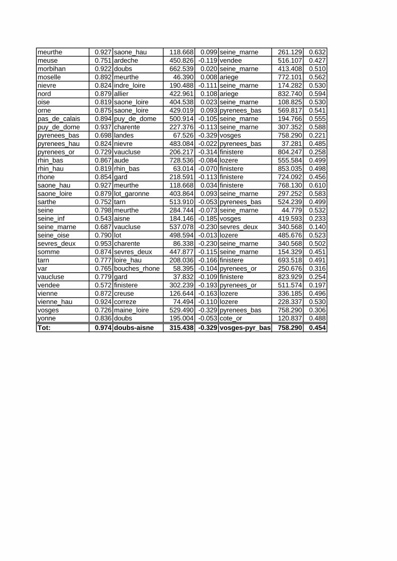
meurthe 0.927 saone_hau 118.668 0.099 seine_marne 261.129 0.632meuse 0.751 ardeche 450.826 -0.119 vendee 516.107 0.427morbihan 0.922 doubs 662.539 0.020 seine_marne 413.408 0.510moselle 0.892 meurthe 46.390 0.008 ariege 772.101 0.562nievre 0.824 indre_loire 190.488 -0.111 seine_marne 174.282 0.530nord 0.879 allier 422.961 0.108 ariege 832.740 0.594oise 0.819 saone_loire 404.538 0.023 seine_marne 108.825 0.530orne 0.875 saone_loire 429.019 0.093 pyrenees_bas 569.817 0.541pas_de_calais 0.894 puy_de_dome 500.914 -0.105 seine_marne 194.766 0.555puy_de_dome 0.937 charente 227.376 -0.113 seine_marne 307.352 0.588pyrenees_bas 0.698 landes 67.526 -0.329 vosges 758.290 0.221pyrenees_hau 0.824 nievre 483.084 -0.022 pyrenees_bas 37.281 0.485pyrenees_or 0.729 vaucluse 206.217 -0.314 finistere 804.247 0.258rhin_bas 0.867 aude 728.536 -0.084 lozere 555.584 0.499rhin_hau 0.819 rhin_bas 63.014 -0.070 finistere 853.035 0.498rhone 0.854 gard 218.591 -0.113 finistere 724.092 0.456saone_hau 0.927 meurthe 118.668 0.034 finistere 768.130 0.610saone_loire 0.879 lot_garonne 403.864 0.093 seine_marne 297.252 0.583sarthe 0.752 tarn 513.910 -0.053 pyrenees_bas 524.239 0.499seine 0.798 meurthe 284.744 -0.073 seine_marne 44.779 0.532seine_inf 0.543 aisne 184.146 -0.185 vosges 419.593 0.233seine_marne 0.687 vaucluse 537.078 -0.230 sevres_deux 340.568 0.140seine_oise 0.790 lot 498.594 -0.013 lozere 485.676 0.523sevres_deux 0.953 charente 86.338 -0.230 seine_marne 340.568 0.502somme 0.874 sevres_deux 447.877 -0.115 seine_marne 154.329 0.451tarn 0.777 loire_hau 208.036 -0.166 finistere 693.518 0.491var 0.765 bouches_rhone 58.395 -0.104 pyrenees_or 250.676 0.316vaucluse 0.779 gard 37.832 -0.109 finistere 823.929 0.254vendee 0.572 finistere 302.239 -0.193 pyrenees_or 511.574 0.197vienne 0.872 creuse 126.644 -0.163 lozere 336.185 0.496vienne_hau 0.924 correze 74.494 -0.110 lozere 228.337 0.530vosges 0.726 maine_loire 529.490 -0.329 pyrenees_bas 758.290 0.306yonne 0.836 doubs 195.004 -0.053 cote_or 120.837 0.488Tot: 0.974 doubs-aisne 315.438 -0.329 vosges-pyr_bas 758.290 0.454

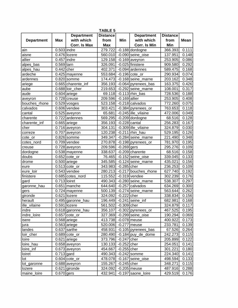
Department Distance Department DistanceDepartment Max with which from Min with which from Mean

Corr. Is Max Max Corr. Is Min Minain 0.503 indre 279.722 -0.188 dordogne 366.393 0.111aisne 0.476 lozere 560.010 -0.090 seine_oise 137.951 0.148allier 0.457 indre 129.158 -0.169 aveyron 253.905 0.086alpes_bas 0.569 tarn 326.091 -0.025 finistere 909.580 0.292alpes_hau 0.442 cher 402.371 -0.094 ardennes 589.475 0.168ardeche 0.425 mayenne 553.684 -0.196 cote_or 290.934 0.074ardennes 0.820 somme 174.473 -0.168 seine_marne 203.162 0.348ariege 0.665 charente_inf 356.193 -0.064 pyrenees_bas 163.375 0.426aube 0.688 loir_cher 219.653 -0.292 seine_marne 108.001 0.317aude 0.604 ariege 69.118 -0.113 rhin_bas 728.536 0.188aveyron 0.728 creuse 209.596 -0.169 allier 253.905 0.408bouches_rhone 0.529 vosges 523.158 -0.218 calvados 772.260 0.075calvados 0.606 vendee 303.421 -0.384 pyrenees_or 763.653 0.118cantal 0.525 aveyron 65.681 -0.245 ille_vilaine 472.006 0.049charente 0.722 ardennes 569.295 -0.209 dordogne 68.516 0.128charente_inf 0.665 ariege 356.193 -0.228 cantal 256.283 0.167cher 0.716 aveyron 304.131 -0.309 ille_vilaine 324.879 0.030correze 0.707 aveyron 120.238 -0.211 rhin_hau 529.195 0.126cote_or 0.826 somme 349.347 -0.284 seine_marne 221.490 0.348cotes_nord 0.709 vendee 270.878 -0.198 pyrenees_or 781.970 0.195creuse 0.728 aveyron 209.596 -0.269 gers 295.276 0.109dordogne 0.538 mayenne 338.637 -0.209 charente 68.516 0.158doubs 0.652 cote_or 76.465 -0.152 seine_oise 339.045 0.133drome 0.500 ariege 345.585 -0.124 seine_marne 435.021 0.156eure 0.513 cote_or 343.983 -0.285 cher 236.253 0.109eure_loir 0.543 vendee 280.213 -0.217 bouches_rhone 627.740 0.192finistere 0.685 cotes_nord 115.552 -0.319 vendee 302.239 0.176gard 0.713 loiret 490.343 -0.280 seine_marne 538.307 0.297garonne_hau 0.651 manche 644.640 -0.257 calvados 634.269 0.300gers 0.724 mayenne 500.139 -0.274 seine_marne 563.644 0.262gironde 0.621 lozere 324.092 -0.222 cher 338.834 0.156herault 0.495 garonne_hau 196.449 -0.241 seine_inf 682.981 0.168ille_vilaine 0.591 lozere 561.502 -0.309 cher 324.879 0.117indre 0.618 garonne_hau 356.107 -0.302 pyrenees_or 467.525 0.195indre_loire 0.657 cote_or 327.369 -0.299 seine_oise 190.294 0.069isere 0.568 ariege 413.738 -0.078 meuse 400.922 0.173jura 0.563 ariege 520.006 -0.277 meuse 233.781 0.139landes 0.637 sarthe 458.931 -0.105 pyrenees_bas 67.526 0.264loir_cher 0.689 cote_or 280.490 -0.184 puy_de_dome 242.273 0.115loire 0.621 ariege 373.796 -0.247 cher 205.899 0.122loire_hau 0.658 aveyron 130.133 -0.252 cher 254.051 0.141loire_inf 0.673 aveyron 454.667 -0.255 cher 301.221 0.180loiret 0.713 gard 490.343 -0.242 somme 224.340 0.141lot 0.604 cote_or 478.078 -0.167 seine_oise 498.594 0.133lot_garonne 0.688 aveyron 155.267 -0.245 cher 348.271 0.115lozere 0.621 gironde 324.092 -0.205 meuse 487.916 0.288maine_loire 0.670 gers 432.941 -0.197 saone_loire 429.519 0.176

TABLE 5

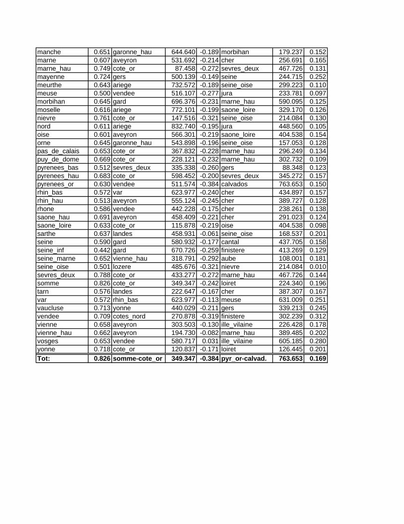
manche 0.651 garonne_hau 644.640 -0.189 morbihan 179.237 0.152marne 0.607 aveyron 531.692 -0.214 cher 256.691 0.165marne_hau 0.749 cote_or 87.458 -0.272 sevres_deux 467.726 0.131mayenne 0.724 gers 500.139 -0.149 seine 244.715 0.252meurthe 0.643 ariege 732.572 -0.189 seine_oise 299.223 0.110meuse 0.500 vendee 516.107 -0.277 jura 233.781 0.097morbihan 0.645 gard 696.376 -0.231 marne_hau 590.095 0.125moselle 0.616 ariege 772.101 -0.199 saone_loire 329.170 0.126nievre 0.761 cote_or 147.516 -0.321 seine_oise 214.084 0.130nord 0.611 ariege 832.740 -0.195 jura 448.560 0.105oise 0.601 aveyron 566.301 -0.219 saone_loire 404.538 0.154orne 0.645 garonne_hau 543.898 -0.196 seine_oise 157.053 0.128pas_de_calais 0.653 cote_or 367.832 -0.228 marne_hau 296.249 0.134puy_de_dome 0.669 cote_or 228.121 -0.232 marne_hau 302.732 0.109pyrenees_bas 0.512 sevres_deux 335.338 -0.260 gers 88.348 0.123pyrenees_hau 0.683 cote_or 598.452 -0.200 sevres_deux 345.272 0.157pyrenees_or 0.630 vendee 511.574 -0.384 calvados 763.653 0.150rhin_bas 0.572 var 623.977 -0.240 cher 434.897 0.157rhin_hau 0.513 aveyron 555.124 -0.245 cher 389.727 0.128rhone 0.586 vendee 442.228 -0.175 cher 238.261 0.138saone_hau 0.691 aveyron 458.409 -0.221 cher 291.023 0.124saone_loire 0.633 cote_or 115.878 -0.219 oise 404.538 0.098sarthe 0.637 landes 458.931 -0.061 seine_oise 168.537 0.201seine 0.590 gard 580.932 -0.177 cantal 437.705 0.158seine_inf 0.442 gard 670.726 -0.259 finistere 413.269 0.129seine_marne 0.652 vienne_hau 318.791 -0.292 aube 108.001 0.181seine_oise 0.501 lozere 485.676 -0.321 nievre 214.084 0.010sevres_deux 0.788 cote_or 433.277 -0.272 marne_hau 467.726 0.144somme 0.826 cote_or 349.347 -0.242 loiret 224.340 0.196tarn 0.576 landes 222.647 -0.167 cher 387.307 0.167var 0.572 rhin_bas 623.977 -0.113 meuse 631.009 0.251vaucluse 0.713 yonne 440.029 -0.211 gers 339.213 0.245vendee 0.709 cotes_nord 270.878 -0.319 finistere 302.239 0.312vienne 0.658 aveyron 303.503 -0.130 ille_vilaine 226.428 0.178vienne_hau 0.662 aveyron 194.730 -0.082 marne_hau 389.485 0.202vosges 0.653 vendee 580.717 0.031 ille_vilaine 605.185 0.280yonne 0.718 cote_or 120.837 -0.171 loiret 126.445 0.201Tot: 0.826 somme-cote_or 349.347 -0.384 pyr_or-calvad. 763.653 0.169

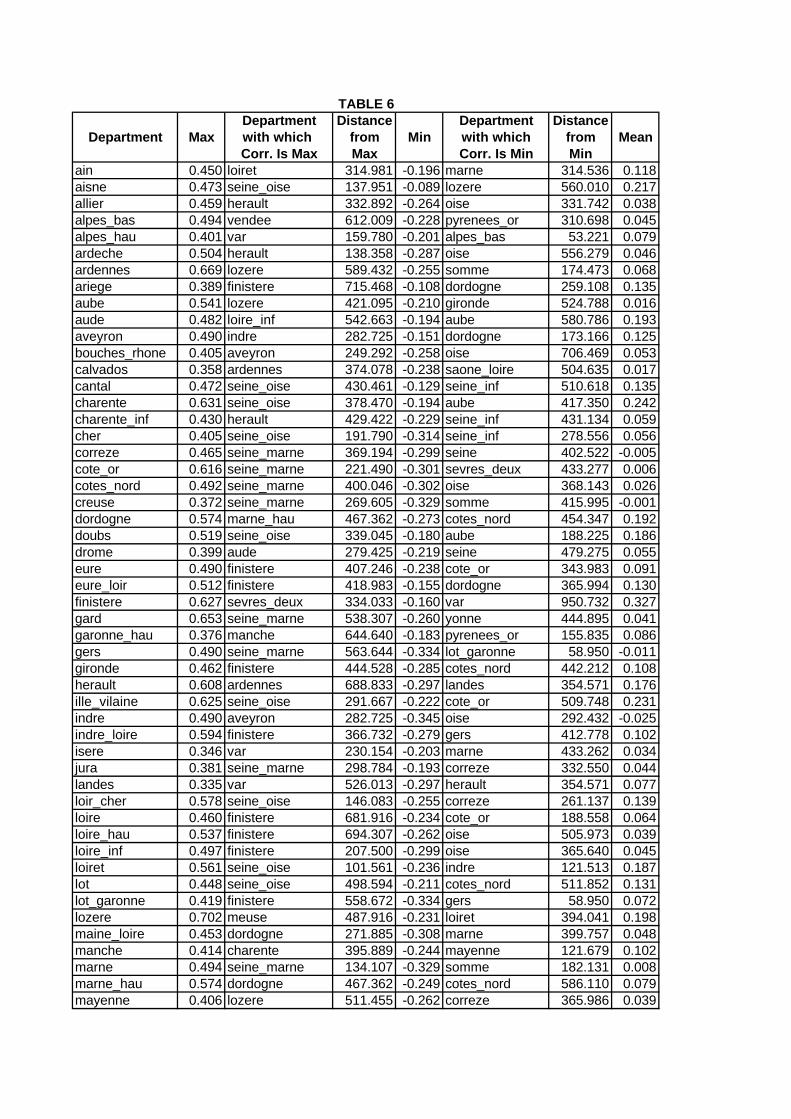
Department Distance Department DistanceDepartment Max with which from Min with which from Mean

Corr. Is Max Max Corr. Is Min Minain 0.450 loiret 314.981 -0.196 marne 314.536 0.118aisne 0.473 seine_oise 137.951 -0.089 lozere 560.010 0.217allier 0.459 herault 332.892 -0.264 oise 331.742 0.038alpes_bas 0.494 vendee 612.009 -0.228 pyrenees_or 310.698 0.045alpes_hau 0.401 var 159.780 -0.201 alpes_bas 53.221 0.079ardeche 0.504 herault 138.358 -0.287 oise 556.279 0.046ardennes 0.669 lozere 589.432 -0.255 somme 174.473 0.068ariege 0.389 finistere 715.468 -0.108 dordogne 259.108 0.135aube 0.541 lozere 421.095 -0.210 gironde 524.788 0.016aude 0.482 loire_inf 542.663 -0.194 aube 580.786 0.193aveyron 0.490 indre 282.725 -0.151 dordogne 173.166 0.125bouches_rhone 0.405 aveyron 249.292 -0.258 oise 706.469 0.053calvados 0.358 ardennes 374.078 -0.238 saone_loire 504.635 0.017cantal 0.472 seine_oise 430.461 -0.129 seine_inf 510.618 0.135charente 0.631 seine_oise 378.470 -0.194 aube 417.350 0.242charente_inf 0.430 herault 429.422 -0.229 seine_inf 431.134 0.059cher 0.405 seine_oise 191.790 -0.314 seine_inf 278.556 0.056correze 0.465 seine_marne 369.194 -0.299 seine 402.522 -0.005cote_or 0.616 seine_marne 221.490 -0.301 sevres_deux 433.277 0.006cotes_nord 0.492 seine_marne 400.046 -0.302 oise 368.143 0.026creuse 0.372 seine_marne 269.605 -0.329 somme 415.995 -0.001dordogne 0.574 marne_hau 467.362 -0.273 cotes_nord 454.347 0.192doubs 0.519 seine_oise 339.045 -0.180 aube 188.225 0.186drome 0.399 aude 279.425 -0.219 seine 479.275 0.055eure 0.490 finistere 407.246 -0.238 cote_or 343.983 0.091eure_loir 0.512 finistere 418.983 -0.155 dordogne 365.994 0.130finistere 0.627 sevres_deux 334.033 -0.160 var 950.732 0.327gard 0.653 seine_marne 538.307 -0.260 yonne 444.895 0.041garonne_hau 0.376 manche 644.640 -0.183 pyrenees_or 155.835 0.086gers 0.490 seine_marne 563.644 -0.334 lot_garonne 58.950 -0.011gironde 0.462 finistere 444.528 -0.285 cotes_nord 442.212 0.108herault 0.608 ardennes 688.833 -0.297 landes 354.571 0.176ille_vilaine 0.625 seine_oise 291.667 -0.222 cote_or 509.748 0.231indre 0.490 aveyron 282.725 -0.345 oise 292.432 -0.025indre_loire 0.594 finistere 366.732 -0.279 gers 412.778 0.102isere 0.346 var 230.154 -0.203 marne 433.262 0.034jura 0.381 seine_marne 298.784 -0.193 correze 332.550 0.044landes 0.335 var 526.013 -0.297 herault 354.571 0.077loir_cher 0.578 seine_oise 146.083 -0.255 correze 261.137 0.139loire 0.460 finistere 681.916 -0.234 cote_or 188.558 0.064loire_hau 0.537 finistere 694.307 -0.262 oise 505.973 0.039loire_inf 0.497 finistere 207.500 -0.299 oise 365.640 0.045loiret 0.561 seine_oise 101.561 -0.236 indre 121.513 0.187lot 0.448 seine_oise 498.594 -0.211 cotes_nord 511.852 0.131lot_garonne 0.419 finistere 558.672 -0.334 gers 58.950 0.072lozere 0.702 meuse 487.916 -0.231 loiret 394.041 0.198maine_loire 0.453 dordogne 271.885 -0.308 marne 399.757 0.048manche 0.414 charente 395.889 -0.244 mayenne 121.679 0.102marne 0.494 seine_marne 134.107 -0.329 somme 182.131 0.008marne_hau 0.574 dordogne 467.362 -0.249 cotes_nord 586.110 0.079mayenne 0.406 lozere 511.455 -0.262 correze 365.986 0.039

TABLE 6

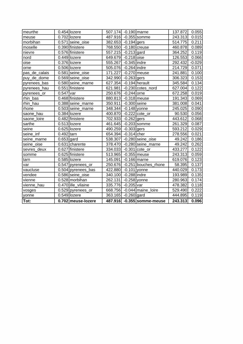
meurthe 0.454 lozere 507.174 -0.190 marne 137.872 0.055meuse 0.702 lozere 487.916 -0.355 somme 243.313 0.015morbihan 0.571 seine_oise 382.653 -0.194 gers 514.775 0.211moselle 0.390 finistere 768.550 -0.180 creuse 460.878 0.089nievre 0.576 finistere 557.215 -0.213 gard 364.252 0.119nord 0.449 lozere 649.679 -0.218 oise 126.553 0.066oise 0.376 lozere 555.267 -0.345 indre 292.432 -0.029orne 0.506 lozere 505.076 -0.264 indre 214.729 0.071pas_de_calais 0.581 seine_oise 171.227 -0.270 meuse 241.881 0.100puy_de_dome 0.569 seine_oise 342.990 -0.263 gers 306.323 0.153pyrenees_bas 0.580 seine_marne 627.354 -0.194 herault 345.584 0.134pyrenees_hau 0.551 finistere 621.981 -0.230 cotes_nord 627.004 0.122pyrenees_or 0.547 var 250.676 -0.244 orne 672.258 0.019rhin_bas 0.468 finistere 880.813 -0.318 meuse 191.343 0.069rhin_hau 0.388 seine_marne 350.911 -0.300 seine 381.008 0.041rhone 0.503 seine_marne 348.344 -0.148 yonne 245.025 0.090saone_hau 0.384 lozere 400.870 -0.222 cote_or 90.530 0.056saone_loire 0.482 finistere 702.933 -0.262 gers 443.612 0.068sarthe 0.513 lozere 461.645 -0.203 somme 261.329 0.087seine 0.625 lozere 490.259 -0.303 gers 593.212 0.029seine_inf 0.492 tarn 654.394 -0.314 cher 278.556 0.021seine_marne 0.653 gard 538.307 -0.280 seine_oise 49.242 0.186seine_oise 0.631 charente 378.470 -0.280 seine_marne 49.242 0.262sevres_deux 0.627 finistere 334.033 -0.301 cote_or 433.277 0.122somme 0.625 finistere 513.965 -0.355 meuse 243.313 0.059tarn 0.585 lozere 145.091 -0.166 marne 619.076 0.123var 0.547 pyrenees_or 250.676 -0.251 bouches_rhone 58.395 0.137vaucluse 0.504 pyrenees_bas 422.880 -0.101 yonne 440.029 0.173vendee 0.586 seine_oise 340.100 -0.288 indre 193.989 0.135vienne 0.528 morbihan 262.131 -0.258 yonne 280.963 0.174vienne_hau 0.470 ille_vilaine 335.776 -0.205 var 478.382 0.118vosges 0.529 pyrenees_or 668.756 -0.044 maine_loire 529.490 0.222yonne 0.549 lozere 363.165 -0.260 gard 444.895 0.119Tot: 0.702 meuse-lozere 487.916 -0.355 somme-meuse 243.313 0.096

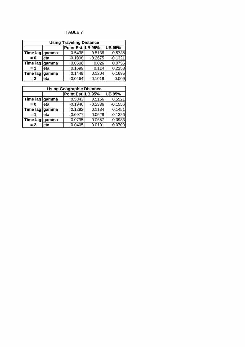
Point Est. LB 95% UB 95%Time lag gamma 0.5438 0.5138 0.5738

= 0 eta -0.1998 -0.2675 -0.1321Time lag gamma 0.0508 0.026 0.0756

= 1 eta 0.1699 0.114 0.2258Time lag gamma 0.1449 0.1204 0.1695

= 2 eta -0.0464 -0.1018 0.009

Point Est. LB 95% UB 95%Time lag gamma 0.5343 0.5166 0.5521

= 0 eta -0.1946 -0.2336 -0.1556Time lag gamma 0.1292 0.1134 0.1451

= 1 eta 0.0977 0.0628 0.1326Time lag gamma 0.0795 0.0657 0.0933

= 2 eta 0.0405 0.0101 0.0709

Using Traveling Distance

Using Geographic Distance

TABLE 7

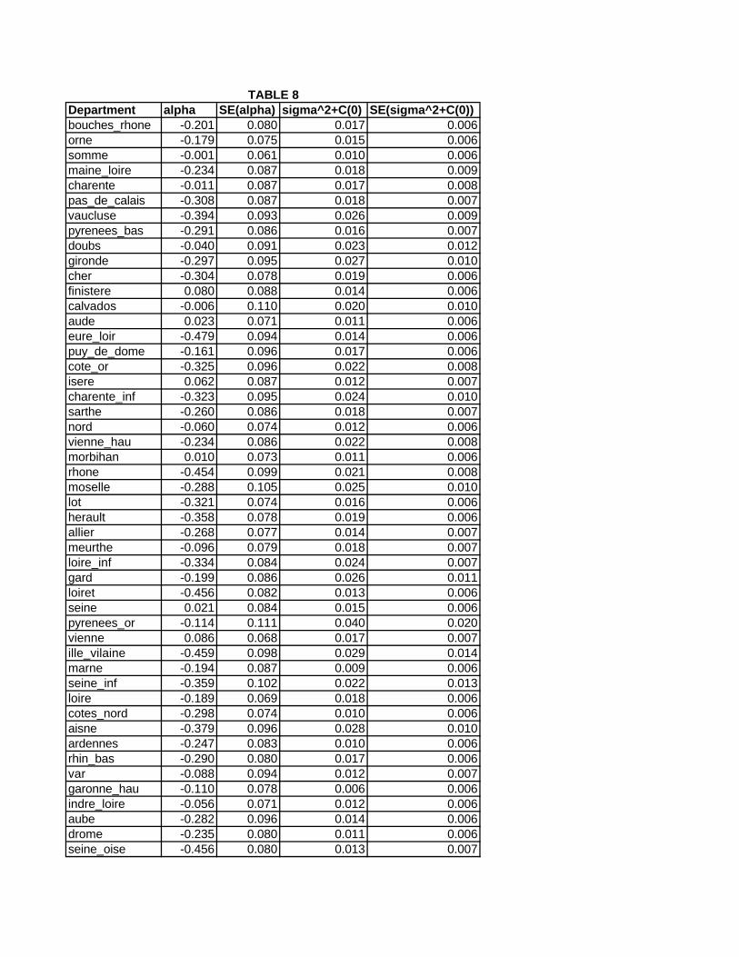
Department alpha SE(alpha) sigma^2+C(0) SE(sigma^2+C(0))bouches_rhone -0.201 0.080 0.017 0.006orne -0.179 0.075 0.015 0.006somme -0.001 0.061 0.010 0.006maine_loire -0.234 0.087 0.018 0.009charente -0.011 0.087 0.017 0.008pas_de_calais -0.308 0.087 0.018 0.007vaucluse -0.394 0.093 0.026 0.009pyrenees_bas -0.291 0.086 0.016 0.007doubs -0.040 0.091 0.023 0.012gironde -0.297 0.095 0.027 0.010cher -0.304 0.078 0.019 0.006finistere 0.080 0.088 0.014 0.006calvados -0.006 0.110 0.020 0.010aude 0.023 0.071 0.011 0.006eure_loir -0.479 0.094 0.014 0.006puy_de_dome -0.161 0.096 0.017 0.006cote_or -0.325 0.096 0.022 0.008isere 0.062 0.087 0.012 0.007charente_inf -0.323 0.095 0.024 0.010sarthe -0.260 0.086 0.018 0.007nord -0.060 0.074 0.012 0.006vienne_hau -0.234 0.086 0.022 0.008morbihan 0.010 0.073 0.011 0.006rhone -0.454 0.099 0.021 0.008moselle -0.288 0.105 0.025 0.010lot -0.321 0.074 0.016 0.006herault -0.358 0.078 0.019 0.006allier -0.268 0.077 0.014 0.007meurthe -0.096 0.079 0.018 0.007loire_inf -0.334 0.084 0.024 0.007gard -0.199 0.086 0.026 0.011loiret -0.456 0.082 0.013 0.006seine 0.021 0.084 0.015 0.006pyrenees_or -0.114 0.111 0.040 0.020vienne 0.086 0.068 0.017 0.007ille_vilaine -0.459 0.098 0.029 0.014marne -0.194 0.087 0.009 0.006seine_inf -0.359 0.102 0.022 0.013loire -0.189 0.069 0.018 0.006cotes_nord -0.298 0.074 0.010 0.006aisne -0.379 0.096 0.028 0.010ardennes -0.247 0.083 0.010 0.006rhin_bas -0.290 0.080 0.017 0.006var -0.088 0.094 0.012 0.007garonne_hau -0.110 0.078 0.006 0.006indre_loire -0.056 0.071 0.012 0.006aube -0.282 0.096 0.014 0.006drome -0.235 0.080 0.011 0.006seine_oise -0.456 0.080 0.013 0.007

TABLE 8

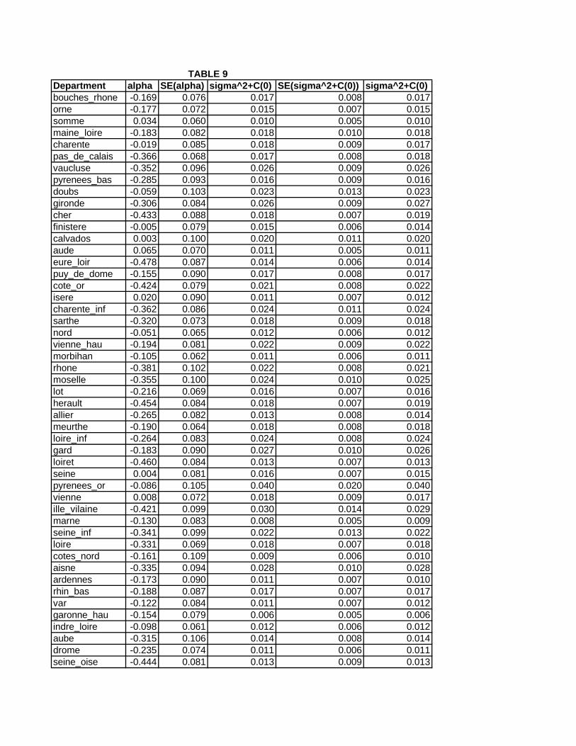
Department alpha SE(alpha) sigma^2+C(0) SE(sigma^2+C(0)) sigma^2+C(0)bouches_rhone -0.169 0.076 0.017 0.008 0.017orne -0.177 0.072 0.015 0.007 0.015somme 0.034 0.060 0.010 0.005 0.010maine_loire -0.183 0.082 0.018 0.010 0.018charente -0.019 0.085 0.018 0.009 0.017pas_de_calais -0.366 0.068 0.017 0.008 0.018vaucluse -0.352 0.096 0.026 0.009 0.026pyrenees_bas -0.285 0.093 0.016 0.009 0.016doubs -0.059 0.103 0.023 0.013 0.023gironde -0.306 0.084 0.026 0.009 0.027cher -0.433 0.088 0.018 0.007 0.019finistere -0.005 0.079 0.015 0.006 0.014calvados 0.003 0.100 0.020 0.011 0.020aude 0.065 0.070 0.011 0.005 0.011eure_loir -0.478 0.087 0.014 0.006 0.014puy_de_dome -0.155 0.090 0.017 0.008 0.017cote_or -0.424 0.079 0.021 0.008 0.022isere 0.020 0.090 0.011 0.007 0.012charente_inf -0.362 0.086 0.024 0.011 0.024sarthe -0.320 0.073 0.018 0.009 0.018nord -0.051 0.065 0.012 0.006 0.012vienne_hau -0.194 0.081 0.022 0.009 0.022morbihan -0.105 0.062 0.011 0.006 0.011rhone -0.381 0.102 0.022 0.008 0.021moselle -0.355 0.100 0.024 0.010 0.025lot -0.216 0.069 0.016 0.007 0.016herault -0.454 0.084 0.018 0.007 0.019allier -0.265 0.082 0.013 0.008 0.014meurthe -0.190 0.064 0.018 0.008 0.018loire_inf -0.264 0.083 0.024 0.008 0.024gard -0.183 0.090 0.027 0.010 0.026loiret -0.460 0.084 0.013 0.007 0.013seine 0.004 0.081 0.016 0.007 0.015pyrenees_or -0.086 0.105 0.040 0.020 0.040vienne 0.008 0.072 0.018 0.009 0.017ille_vilaine -0.421 0.099 0.030 0.014 0.029marne -0.130 0.083 0.008 0.005 0.009seine_inf -0.341 0.099 0.022 0.013 0.022loire -0.331 0.069 0.018 0.007 0.018cotes_nord -0.161 0.109 0.009 0.006 0.010aisne -0.335 0.094 0.028 0.010 0.028ardennes -0.173 0.090 0.011 0.007 0.010rhin_bas -0.188 0.087 0.017 0.007 0.017var -0.122 0.084 0.011 0.007 0.012garonne_hau -0.154 0.079 0.006 0.005 0.006indre_loire -0.098 0.061 0.012 0.006 0.012aube -0.315 0.106 0.014 0.008 0.014drome -0.235 0.074 0.011 0.006 0.011seine_oise -0.444 0.081 0.013 0.009 0.013

TABLE 9

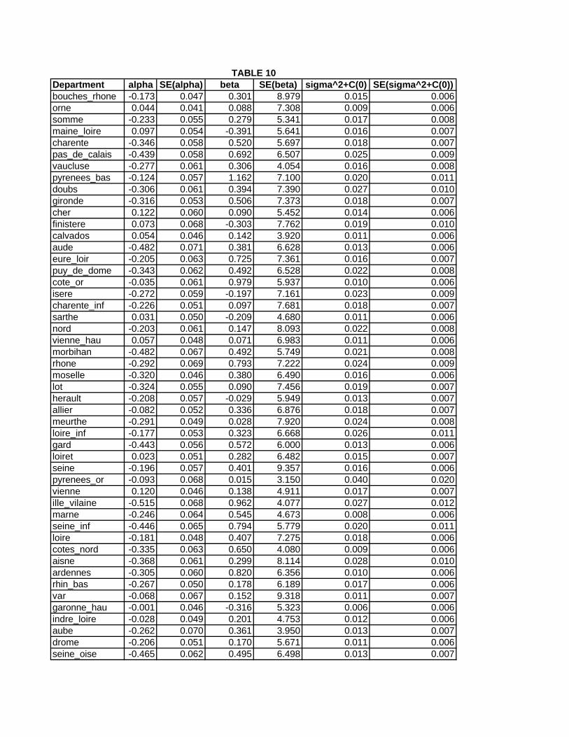
Department alpha SE(alpha) beta SE(beta) sigma^2+C(0) SE(sigma^2+C(0))bouches_rhone -0.173 0.047 0.301 8.979 0.015 0.006orne 0.044 0.041 0.088 7.308 0.009 0.006somme -0.233 0.055 0.279 5.341 0.017 0.008maine_loire 0.097 0.054 -0.391 5.641 0.016 0.007charente -0.346 0.058 0.520 5.697 0.018 0.007pas_de_calais -0.439 0.058 0.692 6.507 0.025 0.009vaucluse -0.277 0.061 0.306 4.054 0.016 0.008pyrenees_bas -0.124 0.057 1.162 7.100 0.020 0.011doubs -0.306 0.061 0.394 7.390 0.027 0.010gironde -0.316 0.053 0.506 7.373 0.018 0.007cher 0.122 0.060 0.090 5.452 0.014 0.006finistere 0.073 0.068 -0.303 7.762 0.019 0.010calvados 0.054 0.046 0.142 3.920 0.011 0.006aude -0.482 0.071 0.381 6.628 0.013 0.006eure_loir -0.205 0.063 0.725 7.361 0.016 0.007puy_de_dome -0.343 0.062 0.492 6.528 0.022 0.008cote_or -0.035 0.061 0.979 5.937 0.010 0.006isere -0.272 0.059 -0.197 7.161 0.023 0.009charente_inf -0.226 0.051 0.097 7.681 0.018 0.007sarthe 0.031 0.050 -0.209 4.680 0.011 0.006nord -0.203 0.061 0.147 8.093 0.022 0.008vienne_hau 0.057 0.048 0.071 6.983 0.011 0.006morbihan -0.482 0.067 0.492 5.749 0.021 0.008rhone -0.292 0.069 0.793 7.222 0.024 0.009moselle -0.320 0.046 0.380 6.490 0.016 0.006lot -0.324 0.055 0.090 7.456 0.019 0.007herault -0.208 0.057 -0.029 5.949 0.013 0.007allier -0.082 0.052 0.336 6.876 0.018 0.007meurthe -0.291 0.049 0.028 7.920 0.024 0.008loire_inf -0.177 0.053 0.323 6.668 0.026 0.011gard -0.443 0.056 0.572 6.000 0.013 0.006loiret 0.023 0.051 0.282 6.482 0.015 0.007seine -0.196 0.057 0.401 9.357 0.016 0.006pyrenees_or -0.093 0.068 0.015 3.150 0.040 0.020vienne 0.120 0.046 0.138 4.911 0.017 0.007ille_vilaine -0.515 0.068 0.962 4.077 0.027 0.012marne -0.246 0.064 0.545 4.673 0.008 0.006seine_inf -0.446 0.065 0.794 5.779 0.020 0.011loire -0.181 0.048 0.407 7.275 0.018 0.006cotes_nord -0.335 0.063 0.650 4.080 0.009 0.006aisne -0.368 0.061 0.299 8.114 0.028 0.010ardennes -0.305 0.060 0.820 6.356 0.010 0.006rhin_bas -0.267 0.050 0.178 6.189 0.017 0.006var -0.068 0.067 0.152 9.318 0.011 0.007garonne_hau -0.001 0.046 -0.316 5.323 0.006 0.006indre_loire -0.028 0.049 0.201 4.753 0.012 0.006aube -0.262 0.070 0.361 3.950 0.013 0.007drome -0.206 0.051 0.170 5.671 0.011 0.006seine_oise -0.465 0.062 0.495 6.498 0.013 0.007

TABLE 10

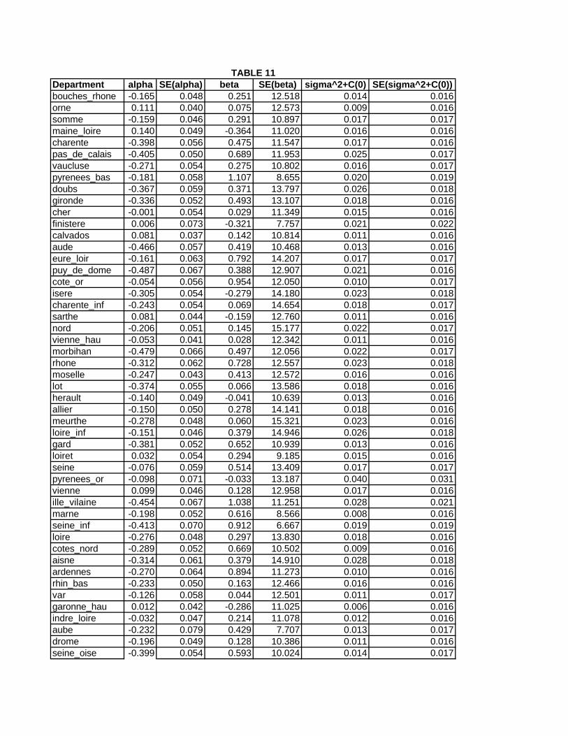
Department alpha SE(alpha) beta SE(beta) sigma^2+C(0) SE(sigma^2+C(0))bouches_rhone -0.165 0.048 0.251 12.518 0.014 0.016orne 0.111 0.040 0.075 12.573 0.009 0.016somme -0.159 0.046 0.291 10.897 0.017 0.017maine_loire 0.140 0.049 -0.364 11.020 0.016 0.016charente -0.398 0.056 0.475 11.547 0.017 0.016pas_de_calais -0.405 0.050 0.689 11.953 0.025 0.017vaucluse -0.271 0.054 0.275 10.802 0.016 0.017pyrenees_bas -0.181 0.058 1.107 8.655 0.020 0.019doubs -0.367 0.059 0.371 13.797 0.026 0.018gironde -0.336 0.052 0.493 13.107 0.018 0.016cher -0.001 0.054 0.029 11.349 0.015 0.016finistere 0.006 0.073 -0.321 7.757 0.021 0.022calvados 0.081 0.037 0.142 10.814 0.011 0.016aude -0.466 0.057 0.419 10.468 0.013 0.016eure_loir -0.161 0.063 0.792 14.207 0.017 0.017puy_de_dome -0.487 0.067 0.388 12.907 0.021 0.016cote_or -0.054 0.056 0.954 12.050 0.010 0.017isere -0.305 0.054 -0.279 14.180 0.023 0.018charente_inf -0.243 0.054 0.069 14.654 0.018 0.017sarthe 0.081 0.044 -0.159 12.760 0.011 0.016nord -0.206 0.051 0.145 15.177 0.022 0.017vienne_hau -0.053 0.041 0.028 12.342 0.011 0.016morbihan -0.479 0.066 0.497 12.056 0.022 0.017rhone -0.312 0.062 0.728 12.557 0.023 0.018moselle -0.247 0.043 0.413 12.572 0.016 0.016lot -0.374 0.055 0.066 13.586 0.018 0.016herault -0.140 0.049 -0.041 10.639 0.013 0.016allier -0.150 0.050 0.278 14.141 0.018 0.016meurthe -0.278 0.048 0.060 15.321 0.023 0.016loire_inf -0.151 0.046 0.379 14.946 0.026 0.018gard -0.381 0.052 0.652 10.939 0.013 0.016loiret 0.032 0.054 0.294 9.185 0.015 0.016seine -0.076 0.059 0.514 13.409 0.017 0.017pyrenees_or -0.098 0.071 -0.033 13.187 0.040 0.031vienne 0.099 0.046 0.128 12.958 0.017 0.016ille_vilaine -0.454 0.067 1.038 11.251 0.028 0.021marne -0.198 0.052 0.616 8.566 0.008 0.016seine_inf -0.413 0.070 0.912 6.667 0.019 0.019loire -0.276 0.048 0.297 13.830 0.018 0.016cotes_nord -0.289 0.052 0.669 10.502 0.009 0.016aisne -0.314 0.061 0.379 14.910 0.028 0.018ardennes -0.270 0.064 0.894 11.273 0.010 0.016rhin_bas -0.233 0.050 0.163 12.466 0.016 0.016var -0.126 0.058 0.044 12.501 0.011 0.017garonne_hau 0.012 0.042 -0.286 11.025 0.006 0.016indre_loire -0.032 0.047 0.214 11.078 0.012 0.016aube -0.232 0.079 0.429 7.707 0.013 0.017drome -0.196 0.049 0.128 10.386 0.011 0.016seine_oise -0.399 0.054 0.593 10.024 0.014 0.017

TABLE 11

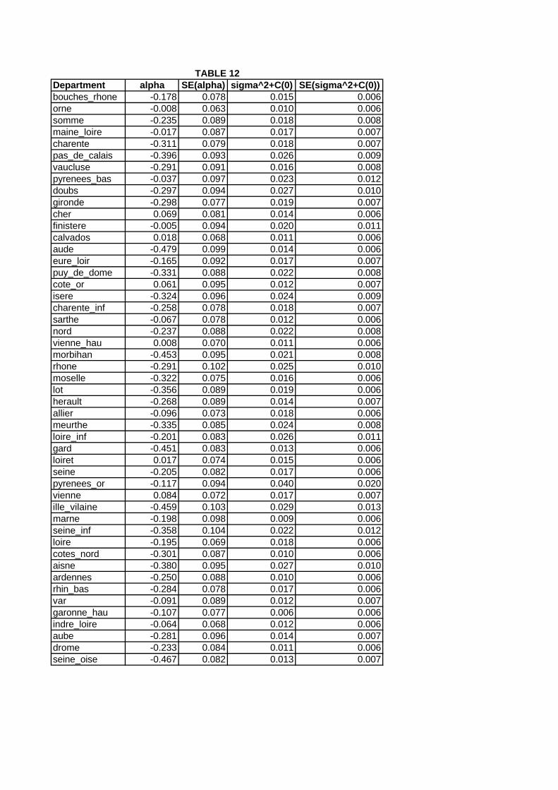
Department alpha SE(alpha) sigma^2+C(0) SE(sigma^2+C(0))bouches_rhone -0.178 0.078 0.015 0.006orne -0.008 0.063 0.010 0.006somme -0.235 0.089 0.018 0.008maine_loire -0.017 0.087 0.017 0.007charente -0.311 0.079 0.018 0.007pas_de_calais -0.396 0.093 0.026 0.009vaucluse -0.291 0.091 0.016 0.008pyrenees_bas -0.037 0.097 0.023 0.012doubs -0.297 0.094 0.027 0.010gironde -0.298 0.077 0.019 0.007cher 0.069 0.081 0.014 0.006finistere -0.005 0.094 0.020 0.011calvados 0.018 0.068 0.011 0.006aude -0.479 0.099 0.014 0.006eure_loir -0.165 0.092 0.017 0.007puy_de_dome -0.331 0.088 0.022 0.008cote_or 0.061 0.095 0.012 0.007isere -0.324 0.096 0.024 0.009charente_inf -0.258 0.078 0.018 0.007sarthe -0.067 0.078 0.012 0.006nord -0.237 0.088 0.022 0.008vienne_hau 0.008 0.070 0.011 0.006morbihan -0.453 0.095 0.021 0.008rhone -0.291 0.102 0.025 0.010moselle -0.322 0.075 0.016 0.006lot -0.356 0.089 0.019 0.006herault -0.268 0.089 0.014 0.007allier -0.096 0.073 0.018 0.006meurthe -0.335 0.085 0.024 0.008loire_inf -0.201 0.083 0.026 0.011gard -0.451 0.083 0.013 0.006loiret 0.017 0.074 0.015 0.006seine -0.205 0.082 0.017 0.006pyrenees_or -0.117 0.094 0.040 0.020vienne 0.084 0.072 0.017 0.007ille_vilaine -0.459 0.103 0.029 0.013marne -0.198 0.098 0.009 0.006seine_inf -0.358 0.104 0.022 0.012loire -0.195 0.069 0.018 0.006cotes_nord -0.301 0.087 0.010 0.006aisne -0.380 0.095 0.027 0.010ardennes -0.250 0.088 0.010 0.006rhin_bas -0.284 0.078 0.017 0.006var -0.091 0.089 0.012 0.007garonne_hau -0.107 0.077 0.006 0.006indre_loire -0.064 0.068 0.012 0.006aube -0.281 0.096 0.014 0.007drome -0.233 0.084 0.011 0.006seine_oise -0.467 0.082 0.013 0.007

TABLE 12

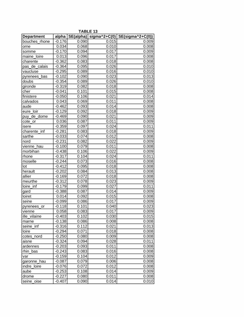
Department alpha SE(alpha) sigma^2+C(0) SE(sigma^2+C(0))bouches_rhone -0.176 0.090 0.015 0.009orne 0.034 0.068 0.010 0.008somme -0.170 0.094 0.017 0.009maine_loire 0.013 0.096 0.017 0.008charente -0.362 0.083 0.018 0.008pas_de_calais -0.364 0.095 0.026 0.010vaucluse -0.295 0.089 0.016 0.010pyrenees_bas -0.102 0.090 0.023 0.013doubs -0.354 0.089 0.026 0.010gironde -0.319 0.082 0.018 0.008cher -0.041 0.101 0.015 0.008finistere -0.050 0.106 0.021 0.014calvados 0.043 0.069 0.011 0.008aude -0.462 0.093 0.014 0.008eure_loir -0.129 0.092 0.018 0.009puy_de_dome -0.469 0.090 0.021 0.009cote_or 0.036 0.087 0.011 0.009isere -0.359 0.097 0.024 0.011charente_inf -0.281 0.083 0.018 0.009sarthe -0.033 0.074 0.012 0.008nord -0.231 0.082 0.022 0.009vienne_hau -0.100 0.079 0.011 0.008morbihan -0.438 0.106 0.022 0.009rhone -0.317 0.104 0.024 0.011moselle -0.244 0.073 0.016 0.008lot -0.412 0.095 0.018 0.008herault -0.202 0.084 0.013 0.008allier -0.169 0.072 0.018 0.008meurthe -0.312 0.078 0.023 0.009loire_inf -0.179 0.099 0.027 0.011gard -0.388 0.087 0.014 0.009loiret 0.014 0.092 0.015 0.008seine -0.099 0.086 0.017 0.009pyrenees_or -0.118 0.101 0.040 0.023vienne 0.058 0.083 0.017 0.009ille_vilaine -0.403 0.102 0.030 0.015marne -0.138 0.086 0.008 0.008seine_inf -0.316 0.112 0.021 0.013loire -0.294 0.071 0.018 0.008cotes_nord -0.250 0.080 0.009 0.008aisne -0.324 0.094 0.028 0.011ardennes -0.203 0.093 0.011 0.008rhin_bas -0.243 0.083 0.016 0.008var -0.159 0.104 0.012 0.009garonne_hau -0.087 0.079 0.006 0.008indre_loire -0.076 0.072 0.012 0.008aube -0.253 0.108 0.014 0.009drome -0.227 0.080 0.011 0.008seine_oise -0.407 0.090 0.014 0.010

TABLE 13

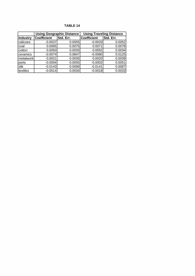
Industry Coefficient Std. Err. Coefficient Std. Err.calicoes -0.0037 0.0055 -0.0033 0.0052coal 0.0065 0.0075 0.0071 0.0078cotton 0.0050 0.0033 0.0052 0.0034ceramics -0.0074 0.0847 -0.0080 0.0125metalwork 0.0021 0.0035 0.0020 0.0039ports -0.0004 0.0055 -0.0002 0.0051silk -0.0143 0.0090 -0.0141 0.0087textiles -0.0014 0.0034 -0.0018 0.0033

Using Geographic Distance Using Traveling Distance

TABLE 14