Cash Settlement of Lean Hog Futures Contracts Reexamined

by

Julieta Frank, Miguel I. Gómez,Eugene Kunda and Philip Garcia

Suggested citation format:

Frank, J., M. I. Gómez, E. Kunda, and P. Garcia. 2008. “Cash Settlement of Lean Hog Futures Contracts Reexamined.” Proceedings of the NCCC-134 Conference on Applied Commodity Price Analysis, Forecasting, and Market Risk Management. St. Louis, MO. [http://www.farmdoc.uiuc.edu/nccc134].

Cash Settlement of Lean Hog Futures Contracts Reexamined

Julieta Frank,

Miguel I. Gómez,

Eugene Kunda and

Philip Garcia*

Paper presented at the NCCC-134 Conference on Applied Commodity Price Analysis, Forecasting, and Market Risk Management

St. Louis, Missouri, April 21-22, 2008

Copyright 2008 by Julieta Frank, Miguel I. Gómez, Eugene Kunda and Philip Garcia. All rights reserved. Readers may make verbatim copies of this document for non-commercial purposes by

any means, provided that this copyright notice appears on all such copies.

________________________ *Graduate Research Assistant, Assistant Professor, Associate Director of the Office for Futures and Options Research, and Professor in the Department of Agricultural and Consumer Economics at the University of Illinois Urbana-Champaign. We would like to thank the Illinois Farm Bureau for partial support of the work.

2

Cash Settlement of Lean Hog Futures Contracts Reexamined

In 1997 the Chicago Mercantile Exchange replaced its live hog futures contract with a cash settlement mechanism based on a Lean Hog Index. Although cash settlement was expected to increase the use of the contract as a hedging tool, producers and packers are concerned that convergence between cash and futures prices is not occurring and that the volatility of the lean hog contract basis has increased in recent years. The purpose of the paper is to reexamine cash settlement of lean hog futures contracts as a hedging tool, focusing on basis behavior and management of basis risk. We also investigate alternative hedging instruments that take into account location differences between regional cash prices and the CME lean hog index. Our results indicate that basis has widened and its variability prior to expiration has increased in the cash settlement period. Nevertheless, there is no evidence that ex-ante basis risk has increased, suggesting that the ability to forecast basis prior to expiration has not decreased with cash settlement. Our findings indicate that a contract on a regional basis can reduce producer price risk and may increase market returns. The benefits of a regional basis appear to accrue from providing the producer with an opportunity to manage the variability in returns associated with both the price level and basis. Keywords: basis behavior, cash settlement, ex-ante basis risk, lean hogs futures contract, regional basis. Introduction Prior to 1997 the Chicago Mercantile Exchange (CME) live hog futures contract was used by hog producers and packers to hedge their hog and pork price risk, and physical delivery settlement facilitated convergence between hog futures and cash prices. In February 1997 the CME changed the structure of the contract by substituting physical delivery with a cash settlement mechanism based on a newly created CME Lean Hog Index. The rationale for the change was to expand the market of the contract as a hedging instrument to domestic and international hog producers and packers as well as to hog and pork importers and exporters. Despite expanded market opportunities, an increasing concern exists among hog producers and packers that convergence between cash and futures prices is not occurring and that the volatility of the lean hog contract basis has increased in recent years.1 These concerns can translate into decreased demand for the contract as a hedging tool, lost marketing opportunities for hog producers and packers, and lower enterprise profitability. Research prior to the lean hog contract suggested that cash settlement would provide better convergence between cash and futures prices, reduce basis variability, and permit effective short-term hedging of cash hogs (Kimle and Hayenga 1994; Ditsch and Leuthold 1996). However recent empirical evidence on the benefits of cash settlement in the hog market case is not clear. For instance, Lien and Tse (1999) show that the lean hog basis became more volatile with cash settlement. More recently, Chan and Lien (2001) find that cash and futures markets have become 1 Meetings with Midwest hog producers support these concerns.

3

less integrated and more segmented after the transition to cash settlement, suggesting that the ability to hedge risk has declined. While the results are likely influenced by the small number of observations during the cash settlement era and the dramatic price changes during the late 1990s, the lean hog contract findings stand in sharp contrast to the impact of cash settlement in other commodities. Producer ability to hedge with lean hog contracts warrants further investigation particularly in the most recent period when adjustment to change in contract specifications is likely completed. In cash settlement contracts the price index employed plays a critical role in hedging effectiveness. For instance, extant literature shows that a cash settlement contract in which the underlying index is an average of different grades has better hedging performance relative to a physical delivery contract because convergence to an average grade generates more stable prices and a more stable basis (Lien 1989; Kahl, Hudson and Ward 1989). Location can also affect the usefulness of a cash settled contract in hedging. Chan and Lien (2001) point out that, if the index is an average of prices at different locations, a broad based index may reduce hedging effectiveness for hedgers outside the index locations or for those in locations with a low weight in the construction of the index. In effect, geographic price differences may mean that the index used for cash settlement is not representative for particular locations. The purpose of the paper is to reexamine cash settlement of lean hog futures contracts as a hedging tool, focusing on basis behavior and management of basis risk. To understand the dimensions of the situation, first we compare hog futures contract basis level, variability, and ex-ante basis risk measured in terms of forecast ability between physical delivery and cash settlement using data from 1985 to 2008 on hog cash and future prices. We then examine the hedging usefulness of the current CME lean hog index and provide an alternative hedging instrument—a regional basis contract—that takes into account location differences between regional cash prices and the CME lean hog index. Our results indicate that basis has widened and its variability prior to expiration has increased in the cash settlement period. However, we find no evidence to suggest that ex-ante basis risk has increased, meaning that the ability to forecast basis prior to expiration has declined little with cash settlement. Routine hedging with futures contracts as expected reduces the variability in returns compared to cash sales. Including location differences further reduces the variability in cash prices. Our results should be of value to users of the hog futures markets and market analysts that offer pricing advice.

Background Change to a cash settled contract was motivated by the CME desire to provide a risk management instrument that was more consistent with the emerging marketing practices in the hog industry. Hog producers were moving from terminal and auction markets to delivering directly to packing plants (Ditsch and Leuthold 1996, Garcia and Sanders 1996, and Kimle and Hayenga 1994). Low volume observed in terminal markets made cash market transactions costly. Changing patterns in cash and futures prices raised concerns about convergence and the effectiveness of hedging activities. The CME responded by providing a lean weight cash settled contract in which the underlying commodity is an index calculated as the two-day weighted

4

average (weighted by the number of head) of individual price indices from the western and eastern corn belt and the mid south regions as reported by USDA (CME, 2008). Cash Settlement and Basis Behavior Research conducted before the introduction of the new contract suggested that the change to a cash settled contract would be beneficial for hedgers. For instance, using simulated data, Kimle and Hayenga (1994) find that the new contract would provide better convergence between cash and futures prices and that basis variability would be significantly reduced. Prior to its implementation, Ditsch and Leuthold (1996) compute optimal hedge ratios and hedging effectiveness measures using a lean hog index computed by the CME. Their results indicate that the cash settled contract would provide better hedging effectiveness for hedging periods ranging from 1 week to six months. Research provides empirical evidence of the benefits of cash settlement in other commodities. For instance, prior to the lean hog contract, the feeder cattle contract moved from physical delivery to cash settlement. In general, research finds that the performance of the contract after the change improved as measured by the stability of the futures price and basis (see Leuthold 1992; Elam 1988; Schroeder and Mintert 1988; Rich and Leuthold 1993; Roswell and Purcell 1990; Schmitz 1997). More recently, Lien and Tse (2002) also find that the cash settlement in feeder cattle decreases the volatility of the futures market which leads to a more stable basis, and a smaller and more stable optimal hedge ratio. Further, Chan and Lien (2003) demonstrate that the futures market has become more stable after cash settlement. In contrast, Kenyon, Bainbridge, and Ernst (1991) find that cash settlement has not significantly changed the basis variance or the basis forecast error when hedging feeder cattle in Virginia; however local cash and futures prices appear to be more highly correlated. While the literature provides evidence of benefits accruing to cash settlement in feeder cattle markets, empirical findings in the hog markets are less supportive. Lien and Tse (1999) find that basis, cash and futures returns become more volatile after the adoption of cash settlement. In addition, Chan and Lien (2001) show that cash settlement leads to a lower contract performance in hog markets. Their results suggest price discovery in the lean hog market was less efficient than in the feeder cattle market after the change. However, their analysis for lean hogs was based on few observations during a period of particularly large market disturbances. Recognizing this limitation, Chan and Lien (2001) re-examined the behavior of the contract removing the first three months of data, but their conclusions remain the same. More recently and using options, Chan and Lien (2004) find that the implied volatility decreases with the cash settlement. Cash Settlement Indices and Hedging Effectiveness Cash settlement contracts in commodity markets haven’t spread as fast as in financial futures because commodity cash markets are composed of submarkets that differ by location and quality, making it difficult to get consistent price quotations which are generally hard to aggregate (Paul 1985). In this context, the accuracy of the index relative to the commercial value of the underlying commodity is critical to contract design and its performance (Garbade and Silber 2001).

5

According to Lien (1989) and Kahl, Hudson, and Ward (1989), hedging effectiveness in cash settlement contracts where the index is an average of different grades is higher than the physical delivery counterpart. This is because physical delivery contracts converge to the cheapest deliverable grade whereas the cash settled contract converges to the average grade which is likely to generate a smaller variance in futures prices. In turn, less variable futures prices lead to a more stable and predictable basis, and therefore to higher hedging effectiveness. Garbade and Silber (2000) conclude that cash settlement contracts improve the risk transfer function of futures markets, give more flexibility in contract design and provide a cost saving alternative as expensive physical delivery on the maturity date is eliminated. Another important consideration in the construction of a cash settlement index is location. Kahl, Hudson, and Ward (1989), for instance, show that in feeder cattle the performance of a cash settlement contract depends on the implementation of an appropriate index. The authors argue that an index based on one location might be useful for producers in that geographical region but it does not reflect accurately prices paid in other locations, whereas an index based on overall averages across regions might not be appropriate for most hedgers facing price differentials beyond transportation costs. As pointed out by Chan and Lien (2001) and Lien and Tse (2006), narrow-based indices are subject to manipulation in thinly traded terminal markets and broad-based indices reduce the hedging effectiveness. Kimle and Hayenga (1994) focus on the construction of the index for hogs. They claim that manipulation can be avoided by including different regions, averaging certain number of days, eliminating price extremes and weighting the price series. Moreover, Paul (1985) argues that a broad index is more consistent and representative of the true price in the underlying market because respondent errors and biases in individual price quotations tend to cancel one another. However, including too many regions or averaging too many days tends to increase basis variability (Kimle and Hayenga 1994). Despite the expectation a cash-settled lean hog contract would lead to better basis behavior and consequently improved hedging effectiveness, empirical work which has focused on price discovery and producer concerns suggest just the opposite. Here, we examine basis behavior directly by describing its behavior before and after the introduction of the lean contract, and then by investigating ex-ante whether the ability to forecast its behavior has changed. We then assess the hedging ability of the lean contract, and examine the hedging effectiveness of a basis contract that accommodates regional price differences relative to the CME lean hog index. Because we use a longer post-introduction period than prior research, our analysis should be less affected by the rather large market disturbances that occurred near the initiation of trading in the lean contract.

Empirical Approach Our empirical approach consists of two parts. First, we compare basis behavior under physical delivery and cash settlement in terms of their magnitudes near expiration, variability prior to expiration, and ex-ante basis risk in terms of forecast ability using data from October 1985 to April 2008. We then examine the hedging usefulness of the current CME lean hog index and

6

provide an alternative hedging instrument—a regional basis contract—that takes into account regional price differences. Basis Behavior The level of the basis during the days prior to expiration influences the attractiveness of hedging opportunities. We employ two measures of basis level: the average level of the basis during a 20 trading day period prior to expiration of contract i in year t ( itB , ) and the level of the basis on the first Wednesday of the expiration month i in year t (BW,t,i). We explain these measures of basis level as a function of the settlement mechanism and the contract month:

it

H

hihit DDcsB ,

310, εααα +++= ∑

=

εt,i ~ N(0, 21σ ) (1)

it

H

hihit DDcsBW ,

310, γβββ +++= ∑

=

γt,i ~ N(0, 22σ ) (2)

where Dcs is a dummy variable for cash settlement (Dcs = 0 before 1997 and Dsc = 1 starting in February, 1997), Di are contract dummy variables (i = 2 is February, i = 4 is April, i = 6 is June, i = 7 is July, i = 8 is August, and i = 10 is December), and εt,i and γt,i are the error terms. Similarly, the variability of the basis plays an important role in any hedge. Predictions for a highly variable basis are likely to be less precise and hedging outcomes become more erratic. To study the effect that the cash settlement contract specification on the basis prior to expiration, we model basis variability for a 20 trading day period before expiration of contract i in year t ( SD(Bt,i )) as a function of the cash settlement contract specification, and the delivery contract month. We use the standard deviation of the basis computed daily as the measure of basis variability. The model is specified as follows,

, 0 1 ,3

( )H

t i h i t ih

SD B Dcs Dδ δ δ υ=

= + + +∑ vt ~ N(0, 23σ ) (3)

where the explanatory variables are the same as in equation (1). Basis Forecasting The use of futures markets for effective hedging relies on the predictability of changes in the basis because such changes determine returns. Garcia and Sanders (1996) use economic and time series models with seasonal dummy variables to forecast the live hog basis and find that both models provide similar basis forecasts. Here we estimate a more direct method that focuses on predicting basis change by the initial level of the basis and other contract characteristics (Tomek 1997). We first specify a time series model with a set of dummy variables accounting for contract month,

7

t

H

hihtt eDBB +++=Δ ∑

=210 δδδ et ~ N(0, 2

4σ ) (4)

where t is the trading day when the hedge is placed, t+j is the first Wednesday of the expiration month, ∆Bt = Bt+j – Bt, Bt+j is the basis on the first Wednesday of the expiration month, Bt is the basis on day t, and et is the error term. Contract month dummy variables are also included as defined in (1) and (2). In a perfect market, the basis at time t would incorporate all of the information in the market and the basis change would reflect exactly convergence between cash and futures ( 0 10, 1δ δ= = − ). In practice, (4) differences can emerge but the procedure allows for a comparative analysis of ex-ante forecast ability. We estimate the model for one-, three- and five-month horizons. For each horizon, we estimate equation (4) for the physical delivery period and the cash settlement period separately. For the one month horizon, Bt is the basis on the first Wednesday of the month prior to the month of expiration, and for the three (five) month horizon, Bt is the basis on the first Wednesday of the third (fifth) month prior to the month of expiration. We employ the estimated standard errors of the regression, 2

4σ) , to examine ex-ante basis risk. Subsequently, we construct F-tests to assess whether ex-ante basis risk increased in the cash settlement period. Moreover, if the F-tests suggest no significant differences in the regression standard errors, we can pool the physical delivery and the cash settlement observations and estimate the following regression

t

H

hihttt eDDcsBDcsBB +++++=Δ ∑

=23210 * δδδδδ et ~ N(0, 2

5σ ) (5)

where Dcs is the cash settlement dummy variable defined in equation (1) and the other terms are the same as in equation (4). We use the estimated coefficients of δ2 and δ3 to evaluate whether the structure of basis forecasting has changed with cash settlement. Marketing strategies and the regional index Convergence of the lean hog futures contract to an index on National hog prices is assured by the cash settlement process at expiration. However, hedgers using the lean hog contract and selling hogs in their local and regional markets are still subject to basis risk with respect to the CME Lean Hog Index, which is a national index based on the US Department of Agriculture reporting system (AMS/USDA 2008a). Further, hedgers no longer have the option of making/taking delivery to arbitrage the difference in prices between the cash and futures markets. Local, regional, and national price differences can influence basis convergence and hedging effectiveness. A regional index may reflect cash prices better and may therefore improve the hedging performance of the contract for that specific region. To examine these issues, we construct a regional index in the same manner as the CME Lean Hog Index but using the USDA “Iowa/Minnesota Daily Direct Prior Day Hog Report Based on Plant Location” (hereafter referred to as the IA/MN Regional Lean Hog Index (AMS/USDA 2008b)). We then assess its performance by comparing mean returns and variability of

8

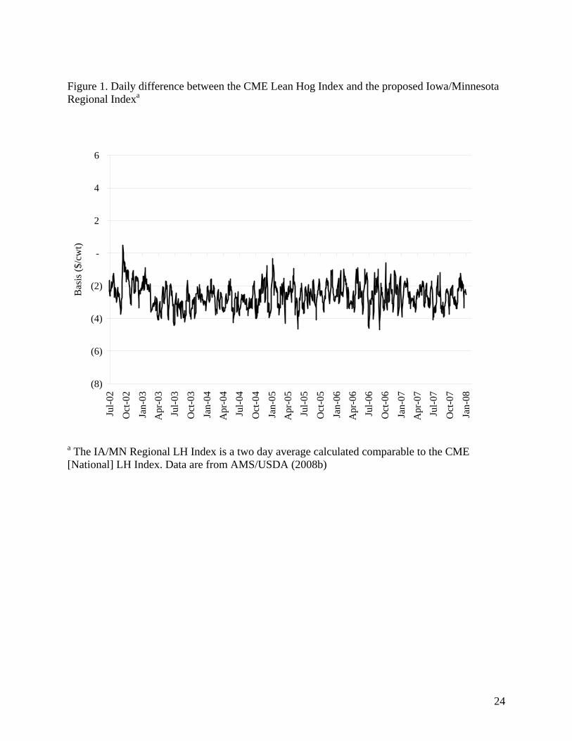
alternative marketing strategies using the regional index relative to other marketing strategies that use the CME Lean Hog Index. The regional index can be used to hedge the component of the total local basis (local cash price minus CME Lean Hog Index) contained in the difference between the regional and national indices (IA/MN Regional Lean Hog Index minus CME Lean Hog Index). The local cash price for the Iowa/Minnesota producer is provided by the Commodity Research Bureau (AMS/USDA 2008c). The resulting difference is defined as a regional basis contract (IA/MN Regional Lean Hog Basis). The regional basis contract cash settles at the difference between the IA/MN Regional Lean Hog Index and the CME Lean Hog Index. The advantage of constructing a regional index is the ability to hedge the basis risk between the regional index and the national index. Figure 1 shows the daily difference between the CME National Index and the IA/MN Regional Lean Hog Index from mid 2002 to the beginning of 2008. Figure 1 suggests considerable differences between the two indices, ranging from $0 to $4 per cwt. This difference is important for the construction of the regional basis contract discussed below.

[Insert Figure 1 here] Five alternative marketing strategies are investigated and hog producer mean returns and their variance are calculated (Table 1). The strategies were constructed using cash settled futures from the CME Lean Hog Index and on the proposed regional index. Cash sales returns represent sales on the first Wednesday of every even month (February, April, June, August, October, and December) for an Iowa/Minnesota (IA/MN) hog producer. The producer’s mean returns are,

1+

==∑

T

t jt

cash

SR

T (6)

where Rcash is the average return to cash sales, and St+j is the spot price every even month.

[Insert Table 1 here] A second strategy represents a hedge placed prior to the cash sales date. The futures contract corresponding to the month in which the cash sale is made is sold to place the hedge and lifted with a purchase on the date of the cash sale. Daily settlement prices are used to place (sell) and lift (buy) the hedge (futures). The average returns for strategy #2 are calculated as

T

FFRR

T

ttjt

cashfuture

∑=

+ −+= 1

)( (7)

where Rfuture is the average return to the hedge using futures for one, three, or five months prior to the date of the cash sale, Ft is the futures price at the beginning of the hedging horizon, Ft+j is the futures price at the end of the hedging period, and T is the number of contracts entering in the simulation.

9

A third strategy is the sale of an IA/MN Regional Basis contract prior to the cash sales date. The IA/MN Regional Basis is the difference between the CME Lean Hog Index and the IA/MN Regional Lean Hog Index. The average daily basis between the IA/MN Regional Lean Hog Index and the CME Lean Hog Index from mid 2002 to the beginning of 2008 is -$2.59/cwt. Since the IA/MN Regional Lean Hog Index is not available prior to mid 2002, an average basis between the IA/MN Lean Hog cash price and the CME Lean Hog futures on the sales dates for mid 1997 through the beginning of 2008 was calculated as -$2.46/cwt. A fairly priced basis contract would reflect the average basis. For this strategy, a selling basis of -$2.50/cwt is used to represent the fairly priced basis. This is a reasonable and conservative assumption based on the historically consistent regional basis. If the IA/MN Regional Basis is less than -$2.50/cwt on the cash sale date, the basis hedge will have a gain in the contract position to offset the weaker basis on the cash sale. The returns from the basis hedge are added to the cash sale returns,

T

BBRR

T

ttjt

cashbasis

∑=

+ −+= 1

)( (8)

where Rbasis is the average return of the hedge using the basis, Bt+j is the IA/MN Regional Lean Hog basis price at the time of cash sale, and Bt is the basis, -$2.50/cwt, for either one, three, or five months prior to the date of the cash sale. The basis hedge provides basis risk protection but not price risk protection. A fourth strategy is a combination of the national price hedge and regional basis hedge strategies. This strategy would be comparable to a hedge on a futures contract that cash settled to the IA/MN Regional Lean Hog Index instead of the CME Lean Hog Index. The combination of a national price and regional basis hedge creates a synthetic regional price hedge.

regional futures basis cashR R R R= + − (9) Using the strategies as defined above, Rcash is subtracted because it is included in both Rfutures and Rbasis formulas. The fifth strategy is the purchase of an at-the-money IA/MN Regional Basis Put Option prior to the cash sales date. The IA/MN Regional Basis is the difference between the CME Lean Hog Index and the IA/MN Regional Lean Hog Index. Recalling the average basis between the IA/MN Lean Hog cash price and the CME Lean Hog futures on the sales dates from mid 1997 to the beginning of 2008 was -$2.46/cwt, the appropriate ATM option would have a strike price of -$2.50/cwt. Using the options pricing model for a spread the premium is estimated at $0.30/cwt for one-month prior to expiration (Kirk and Aron 2005). This premium may be slightly over-priced as the average basis is slightly more, i.e., out-of-the-money, than the closest strike price we are using for the ATM strike. This is mismatching is inevitable as strike prices are customarily only listed in discrete intervals and the closest strike price must be chosen. The spread option model uses 30% annualized volatility for both indices and 98% correlation between the national and regional lean hog indices. If the IA/MN Regional Basis is less than -$2.50/cwt on the cash sale date, the intrinsic value, SP – national lean hog index, is added to the

10

cash sale returns.

( )( )( )1

max 0, + + +=

− + − −= +

∑T

t t j t j t jt

Boption cash

B BP M IR R

T (10)

where RBoption is the average return of the hedge using the basis option, It+j is the national lean hog index price at the time of cash sale, Mt+j is the IA/MN regional lean hog index price at the time of cash sale, BPt+j is the strike price of the basis option, -$2.50/cwt, and Bt is the basis option premium, $0.30/cwt, $0.50/cwt, or $0.70/cwt, for either one, three, or five months prior to the date of the cash sale, respectively. Data We use spot and futures price data for hogs corresponding to the period 1985-2008 from the Commodity Research Bureau. Spot prices are for Iowa/Minnesota. Spot prices for other regions are taken from USDA Livestock & Grain Market News and are only available starting in 2001 when mandatory reporting came into effect. We transform the series prior to the change to carcass weight by multiplying by a factor of 1.35. Contract months during the entire period of study are February, April, June, July, August, October and December. To construct the series for the basis behavior models (1), (2) and (3), we use daily spot and settlement futures prices for a period of 20 days prior to expiration of each contract. We compute the daily basis and its standard deviation for each 20-day period which yields 68 observations for the period 1985-1996 and 68 observations for the period 1997-2008. To assess basis predictability models (4) and (5), we collected prices for the first Wednesday of each contract month. When a Wednesday was not available we use the following Thursday’s price. We consider three hedging horizons: one, three, and five months. The one-month horizon represents hog producers who are in the last production stage, finishing the animal and anticipating near-term sales. The five-month horizon matches the hog production process and focuses on producers who make decisions at an early stage in the production process. Data sets for the forecasting model (5) were constructed to ensure equally spaced observations and non-overlapping data. For the one-month horizon we use the February, April, June, August, October, and December contracts. For the three-month horizon we examine two ways of constructing the dataset, using April, August, and December contracts, and using June, October, and February contracts. For the five-month horizon we use the three sets of contracts, June-December, February-August, and April-October. We test for possible autocorrelation processes to assess the validity of using overlapping data to gain statistical power to test for differences in basis forecasting between physical delivery and cash settlement. In the presence of autocorrelation we correct using Newey-West standard errors. The basis is computed as spot minus futures prices. For example, the January basis at time t using the February contract is the cash price of the first Wednesday of January minus the futures price for the February contract trading the first Wednesday of January. The basis at time t+j is

11

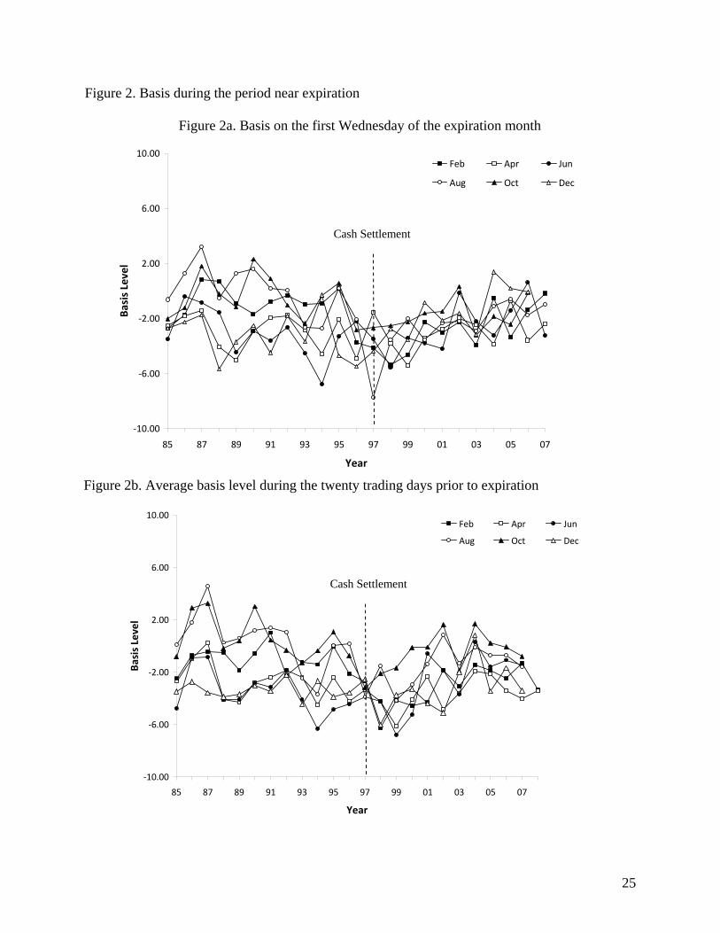
the difference between the cash and the February future price, both collected on the first Wednesday of February. For the hedging analysis we also use the data for the first Wednesday of the contract months listed above with the same 1-, 3-, and 5-month horizons. Results Basis Level Prior to Expiration Figure 2 shows the basis on the fifth day prior to expiration and the average basis during the 20 trading days prior to expiration for the February, April, June, August, October and December contracts. The figure shows that the basis level close to expiration varies over time and across contracts. In general, Figure 2a suggests that the basis widened in the late1990s for most contract months; however, after 2000 the difference between cash and future prices five days prior to expiration appeared to become smaller and comparable to the physical delivery period. The average basis during the 20 trading days prior to expiration shown in Figure 2b suggests a similar basis behavior during the period of analysis.

[Insert Figure 2 here] Table 2 compares the level of the basis before and after the cash settlement contract for each contract month. The top part of the table shows the basis computed the first Wednesday of the expiration month (BW) as a measure of convergence when the contract approaches expiration. The second part shows the average basis for the 20 trading days (approximately one calendar month) before expiration ( B ). We test for significant differences between the two periods (physical delivery versus cash-settlement) using parametric and non-parametric procedures.

[Table 2 here] Results are consistent across the parametric and non-parametric procedures. A comparison between the physical delivery and cash settlement periods indicates that the pooled basis level on the first Wednesday of the expiration month has become wider and more negative with cash settlement, from -$1.42 to -$2.62 per cwt. These differences are driven primarily by the February (-$1.50 versus -$2.84 per cwt), July (-$0.07 versus -$3.75 per cwt), August ($0.46 versus -$2.20 per cwt) and October ($1.19 versus -$0.88 per cwt) contracts. An examination of the average basis on the twenty trading days before expiration, B , yields comparable results. B became wider and more negative during the cash settlement period for the February and August contracts (-$1.05 versus -$3.11 and $0.44 versus -$1.60 per cwt, respectively). The average basis level for October changed from positive ($0.74 per cwt) to negative (-$0.58), but did not became wider with cash settlement. The pooled average basis B indicates that the basis level widened and became more negative by $1 per cwt during the cash settlement period. Overall, results in Table 2 suggest that the basis near expiration became wider and more negative with cash settlement, although not for all contract months. To further examine basis behavior near expiration, Table 3 provides the parameter estimates for equations (1) and (2) using the ending basis BW and tB . The intercepts in Table 3 represent the

12

December contract of the physical delivery period. The main result from Table 3 is that basis level widened during the cash settlement period relative to its physical delivery counterpart. Specifically, the estimated coefficients suggest that the basis increased (and became more negative) by -$1.15 and -$0.99 per cwt during the cash settlement period for BW and tB , respectively. The parameter estimates indicate that the basis levels vary substantially across contract months. For example, the December and June contracts have the most negative basis. The basis level of other contracts tends to be narrower. Overall, results in Table 3 provide additional evidence that during the cash settlement period the basis level became more negative.

[Insert Table 3 here] Basis Variability Prior to Expiration Figure 3 shows the standard deviation of the basis during the twenty trading days prior to expiration, SD( tB ), for the February, April, June, August, October and December contracts. The figure indicates that basis variability varies across contracts and years, roughly ranging from 0.5 to 2.5, except for three contracts in 2004 (June, October, and December) that exhibit higher standard deviations close to four. A possible explanation for this unusually high variability is related to the impact of BSE on US beef exports. During the second semester of 2004, US beef exports were nearly zero, leading to a strong unanticipated growth of US pork exports. Therefore, it is possible that futures did not anticipate the unexpected behavior of cash prices during the second part of 2004 (Lawrence 2008). Except for these three observations, there are no evident differences on basis variability between the cash settlement and physical delivery periods.

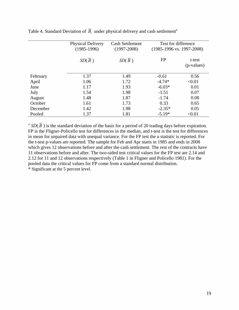
[Insert Figure 3 here] Table 4 provides a comparison of the standard deviation of tB , SD( tB ), between physical delivery and cash settlement periods. Similar to the analysis of basis levels, we test for significant differences between the two periods using parametric and non-parametric procedures. Pooling the contracts, Table 4 suggests that the basis became more variable with the lean hog contract (average SD( tB )) equal 1.37 and 1.81 before and after adoption of cash settlement, respectively). Examination of individual contracts indicates that the difference in the standard deviation of tB is driven by the April, June and December contracts. However, these results should be interpreted with caution, because it is possible that the unusual behavior of cash prices in the second semester of 2004 explained above influences the test results.

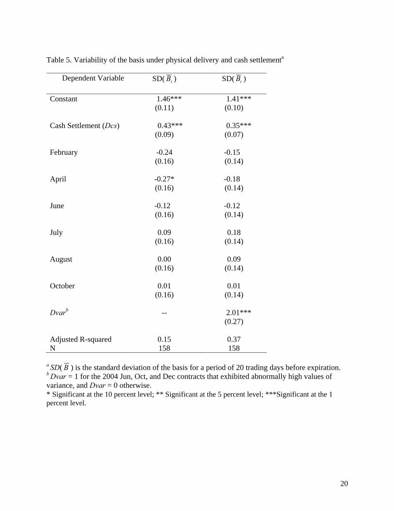
[Insert Table 4 here] To further assess variability of the basis, Table 5 shows the estimated coefficients for the variability model, equation (3). Similar to the basis level analysis the explanatory variables in the first column include a cash settlement and contract month variables. In addition, the regression in the second column incorporates a dummy variable for the 2004 June, October, and December contracts (Dvar). The coefficient of the cash settlement variable is positive and significant, indicating that during the cash settlement period the standard deviation of the basis during the

13

period prior to expiration increased by 0.43 relative to the physical delivery period. Controlling for the unusual behavior of the basis in 2004, the results indicate that the basis in the cash settlement period has a standard deviation $0.35/cwt higher than during the physical delivery contract. Interestingly, none of the contract month variables were significant, except for the April contract in the first column. This suggests that basis variability prior to expiration is comparable across contract months. We tried alternative specifications of the model with various interactions between the cash settlement dummy, the trend, and the contract months, but the results remained the same—basis variability prior to expiration increased after the adoption of cash settlement.

[Insert Table 5 here] Ex-ante Basis Risk To examine ex-ante basis risk we calculate ordinary least squares (OLS) estimates corresponding to equation (4) for the one-, three-, and five-month horizons. We first use non-overlapping and pooled data to obtain the OLS estimates for the physical delivery and cash settlement periods separately. We then use the estimated variance of the regressions of each period to conduct F-tests and examine ex-ante basis risk during the cash settlement period (Table 6). The pooled results indicate that the standard deviations of the errors are moderately higher in the cash settlement period, but not statistically different than the standard deviation of the errors in the physical delivery period. The results are similar for the disaggregate (non-overlapping) equations. The F-tests of employing non-overlapped data indicate that in most cases (except for the April-August-December and the June-December combinations) the standard deviations of the errors are slightly higher in the cash settlement period. Nevertheless, none of these differences are statistically significant. Overall, these results indicate that ex-ante basis risk did not change with cash settlement.

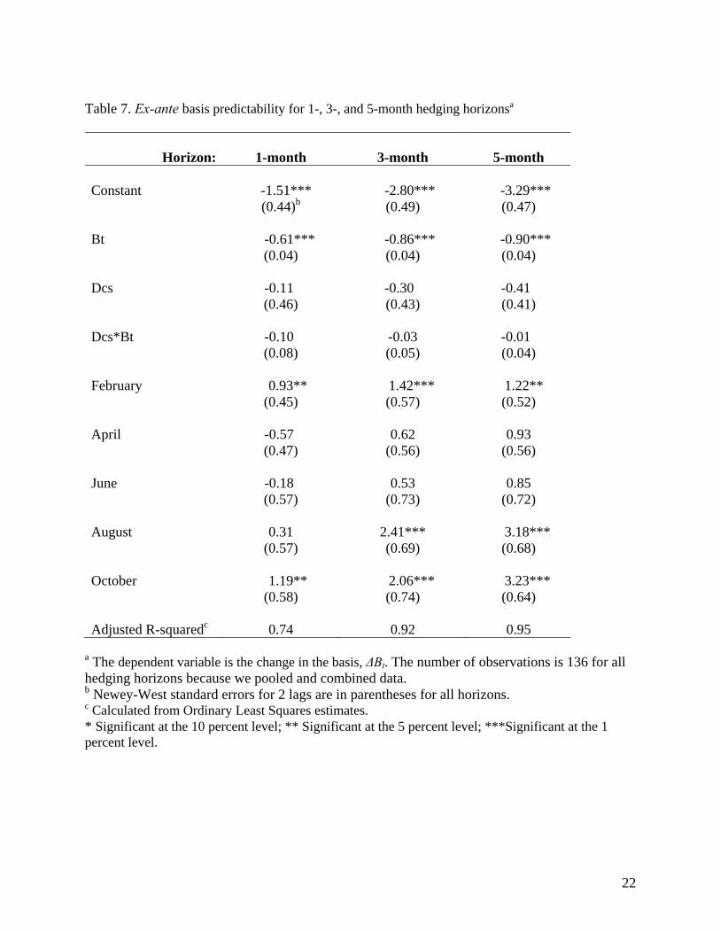
[Insert Table 6 here] In Table 7 we present fitted estimates for equation (5) pooling across contracts and settlement procedures for alternative hedging horizons (one, three and five months). We pooled the physical delivery and cash settlement periods because the results in Table 6 indicate that the standard deviations of the errors between periods do not differ, but use Newey-West standard errors to account for the autocorrelation due to pooling.2 As identified, the basis is perfectly predictable if the estimated intercept equals zero and if the coefficient of the initial basis (Bt) equals -1. The

2 We tested for possible autocorrelation processes using equally-spaced, non-overlapped data for each period. We did not identify autoregressive processes in the physical delivery period. In contrast, an autoregressive structure for the cash settlement period emerged for almost all horizons. Including lagged basis and basis change variables eliminated the autoregressive structure in the error terms, and in some cases resulted in smaller forecast errors in the cash settlement period than in the physical delivery period. Since we focus on the ex-ante basis forecasting, we present results for equation (5) combining data and employing Newey-West standard errors. However, notice the results do indicate a change in the recent dynamics of basis behavior, and suggest that basis in the future can be better forecast in this context.

14

cash settlement variable (Dcs) and its interaction with Bt allow us to assess whether the structure of basis predictability changed in the cash settlement period.

[Insert Table 7 here] For the one-month horizon, the estimated coefficients of the constant (which reflects the December contract) and Bt are significant and equal to -1.51 and -0.61, respectively. Our results show that the coefficient of Bt becomes closer to -1 while the intercept gets farther away from zero for longer hedging horizons. The estimated coefficients of the cash settlement dummy variable are negative, driving the intercept farther away from zero, but are statistically insignificant. In addition, the estimated coefficients of the interaction between the cash settlement variable and Bt are negative for all hedging horizons, making the slopes become closer to -1, but are statistically insignificant. The contract month variables suggest that the intercept becomes closer to zero in the February and October contracts for all three horizons, and in the August contract at the three- and five-month horizon. Similarly, the contract variables suggest little difference between the intercept measures of the April, June and December contracts. The modest forecast differences between periods are illustrated in Figure 4, where the estimated values of the coefficients are mapped net of the monthly effects. Overall, our results show that basis forecasting did not improve, nor worsen in the cash settlement period.

[Insert Figure 4 here] Marketing strategies and the regional index Mean returns and variance of the five simulated hedging strategies are shown in Table 8. The baseline revenue for comparing the hedging strategies is the cash only sale strategy. For the 1997-2008 period, there were 64 observations of sales, with an average cash price of $57.38/cwt and a standard deviation of $12.06/cwt. For all horizons, the mean returns of the option on basis hedges (strategy #5) were largest, except #2 for the three-month horizon. In this context, the options on the basis strategy performed well which may simply reflect the notion that options strategies can result in upside gains while limiting losses. All the futures and options strategies for the horizons showed less risk than the cash only strategy, except #2 for the one-month hedge on futures. The hedges based on the regional index using national price and regional basis had a lower risk for all horizons than strategy #2, a futures price hedge alone. Strategy #4, based on hedging the regional price (futures plus regional basis) had the lowest risk, except the hedge on basis for the one-month horizon.

[Insert Table 8 here] The findings of higher returns and reduced risk from the introduction of regional basis futures and options contracts have implications for hedgers and exchanges. Our findings identify the benefit of listing additional price risk management tools that region specific. It is important to note that liquidity and price discovery of the national market may not fragmented by competing contracts but rather stimulated as regional hedges are placed using both the national price and regional basis contracts. In addition, the analysis suggests considerable benefit from options on the regional basis.

15

Concluding Remarks Cash settlement contracts can stabilize prices because the underlying index is an average of cash prices at different locations, suggesting the basis would be more stable and predictable, and hedging effectiveness would increase. We assess the effect of the cash settlement contract using an expanded dataset of eleven years after its implementation. Our analysis focuses on basis behavior when the contract approaches expiration, changes in its predictability over the hedging period, and the performance of an alternative hedging instrument aimed at overcoming some of the difficulties encountered in the contract’s underlying national index. Our analysis for the lean hog contract suggests that basis level and basis variability increased during the cash settlement period relative to its physical delivery counterpart. Despite wider basis levels and increased variability, the results indicate that the ability to forecast the basis ex-ante at contract expiration has not worsened, nor improved during cash settlement. Conceptually the difference in these findings highlights the importance of the use of an ex-ante decision-making process, and appropriate measures that focus on predictive error to reflect risk. However, in the absence of simple forecasting procedures, producers and market participants may in practice experience additional variability in their returns. Here, we investigate the use of futures, basis, and options to identify useful strategies for producers to manage price risk. Specifying a contract on a regional basis appears to reduce producer price risk and may increase market return. The benefits appear to accrue from providing the producer with an opportunity manage the variability in returns associated with both the price level and basis. Our findings particularly in an ex-post context seem to support recent empirical work that suggests that the cash settlement behavior in the hog market differed from expectations and from behavior in other markets. An explanation for the observed higher basis levels and higher basis variability prior to expiration identified may exist in the recent changes in the hog industry. The industry has gradually become vertically integrated and the volume of hogs negotiated in cash markets is becoming smaller. For instance, in 2001 the number of producer negotiated slaughter hogs was roughly equal to the number of packer-owned slaughter hogs (AMS/USDA 2008a). By 2008 packer-owned slaughtered hogs have nearly doubled, reaching monthly volumes above 2.5 million head, while producer-negotiated volume have declined to as low as to 750,000 head per month. This pattern is relevant as reduced hog numbers accompanied by more variable quality often experienced in declining cash markets (Tomek 1980) may lead to more volatile prices, poorer price discovery and reduced hedging effectiveness. In effect, low volumes of hogs entering the market may be affecting the behavior of the lean hog contract. Part of the increased variability in the cash price can be addressed through the use of the regional basis contract proposed here. Nevertheless, future research should address the relationship between basis behavior and industry structure as more data become available.

16

Table 1. Description of Lean Hog Marketing Strategies

Strategy Explanation of strategy #1

Cash Sale, no hedging

Sale on first Wednesday of every other month from 1997 to the beginning of 2008. (Feb, Apr, Jun, Aug, Oct, Dec)

#2 Hedged with futures on national cash prices

Hedge is placed on the first Wednesday of the month one, three, or five months prior to the sales date. The hedge uses the futures contract that cash settles to the CME Lean Hog Index. (Feb, Apr, Jun, Aug, Oct, Dec)

#3 IA/MN Regional Basis IA/MN Index – CME Index is the IA/MN Basis. Hedge is placed on the basis only. The hedge uses the regional basis contract that cash settles to the difference between the CME Lean Hog Index and the proposed IA/MN Regional Lean Hog Index. An average IA/MN Basis of -$2.50/cwt is used when placing the hedge.

#4 Hedged with futures on regional cash prices

Hedge using futures on national cash prices and IA/MN regional basis to replicate a hedge on regional cash prices. It combines the futures and basis hedges of Strategies #2 and #3, and is comparable to a hedge using a futures contract that cash settles on the IA/MN Regional Lean Hog Index. CME Index + IA/MN Basis = IA/MN Index

#5 IA/MN Regional Basis Option

The hedge is placed using an options on the proposed IA/MN Regional Lean Hog basis. IA/MN Index – CME Index is the IA/MN Basis. The Strike Price is -$2.50/cwt, Premiums are $0.30/cwt, $0.50/cwt, and $0.70/cwt for the one-, three-, and five- month periods.

17

Table 2. Level of the basis under physical delivery and cash settlement ($/cwt)a

Physical Delivery Cash Settlement Test for Differences (1985-1996) (1997-2008) (1985-1996 vs. 1997-2008) BW BW FP t-test (p-

values) February -1.50 -2.84 1.79 0.07 April -2.66 -3.23 0.73 0.35 June -3.86 -3.40 -0.72 0.64 July -0.07 -3.75 4.30* <0.01 August 0.46 -2.20 3.01* 0.01 October 1.19 -0.88 2.77* 0.02 December -3.40 -1.98 -1.21 0.14 Pooled -1.42 -2.62 3.00* <0.01 B B FP t-test February -1.05 -3.11 5.48* <0.01 April -2.70 -3.63 1.07 0.10 June -3.41 -2.73 -0.85 0.43 July -0.37 -1.82 1.01 0.12 August 0.44 -1.60 3.21* 0.02 October 0.74 -0.58 1.62 0.06 December -3.38 -3.17 -0.40 0.72 Pooled -1.40 -2.40 2.66* <0.01

a BW is the basis (St – Ft) on the first Wednesday of the expiration month, B is the average basis of the 20–trading-day period before expiration, FP is the Fligner-Policello test for differences in the median, and t-test is the test for differences in mean for unpaired data with unequal variance. For the FP test the u statistic is reported. For the t-test p-values are reported. The sample for Feb and Apr starts in 1985 and ends in 2008 which gives 12 observations before and after the cash settlement. The rest of the contracts have 11 observations before and after. The two-sided test critical values for the FP test are 2.14 and 2.12 for 11 and 12 observations respectively (Table 1 in Fligner and Policello 1981). For the pooled data the critical values for FP come from a standard normal distribution. * Significant at the 5 percent level.

18

Table 3. Level of the basis under physical delivery and cash settlement

Dependent Variable BWt tB

Cash Settlement (Dcs) -1.15***

(0.34)

-0.99*** (0.27)

February 0.58

(0.63)

1.26** (0.50)

April -0.16

(0.63)

0.14 (0.50)

June -0.85

(0.64)

0.24 (0.51)

July 0.87

(0.64)

2.21*** (0.51)

August 1.91***

(0.64)

2.73*** (0.51)

October 2.85***

(0.63)

3.32*** (0.50)

Constant -2.20***

(0.47)

-2.81*** (0.38)

Adjusted R-squared 0.25 0.37 N 158 158

* Significant at the 10 percent level; ** Significant at the 5 percent level; ***Significant at the 1 percent level.

19

Table 4. Standard Deviation of tB under physical delivery and cash settlementa

Physical Delivery Cash Settlement Test for difference (1985-1996) (1997-2008) (1985-1996 vs. 1997-2008) SD( B ) SD( B ) FP t-test

(p-values)

February 1.37 1.49 -0.61 0.56 April 1.06 1.72 -4.74* <0.01 June 1.17 1.93 -6.03* 0.01 July 1.54 1.98 -1.51 0.07 August 1.48 1.87 -1.74 0.08 October 1.61 1.73 0.33 0.65 December 1.42 1.98 -2.35* 0.05 Pooled 1.37 1.81 -5.19* <0.01

a SD( B ) is the standard deviation of the basis for a period of 20 trading days before expiration. FP is the Fligner-Policello test for differences in the median, and t-test is the test for differences in mean for unpaired data with unequal variance. For the FP test the u statistic is reported. For the t-test p-values are reported. The sample for Feb and Apr starts in 1985 and ends in 2008 which gives 12 observations before and after the cash settlement. The rest of the contracts have 11 observations before and after. The two-sided test critical values for the FP test are 2.14 and 2.12 for 11 and 12 observations respectively (Table 1 in Fligner and Policello 1981). For the pooled data the critical values for FP come from a standard normal distribution. * Significant at the 5 percent level.

20

Table 5. Variability of the basis under physical delivery and cash settlementa

Dependent Variable SD( tB ) SD( tB )

Constant 1.46***

(0.11)

1.41*** (0.10)

Cash Settlement (Dcs) 0.43***

(0.09)

0.35*** (0.07)

February -0.24

(0.16)

-0.15 (0.14)

April -0.27*

(0.16)

-0.18 (0.14)

June -0.12

(0.16)

-0.12 (0.14)

July 0.09

(0.16)

0.18 (0.14)

August 0.00

(0.16)

0.09 (0.14)

October 0.01

(0.16)

0.01 (0.14)

Dvarb -- 2.01***

(0.27)

Adjusted R-squared 0.15 0.37 N 158 158

a SD( B ) is the standard deviation of the basis for a period of 20 trading days before expiration. b Dvar = 1 for the 2004 Jun, Oct, and Dec contracts that exhibited abnormally high values of variance, and Dvar = 0 otherwise. * Significant at the 10 percent level; ** Significant at the 5 percent level; ***Significant at the 1 percent level.

21

Table 6. Ex-Ante basis risk under physical delivery and cash settlement Physical Delivery Cash Settlement Test

Horizon

Standard Deviation

Adjusted R-squared

Standard Deviation

Adjusted R-squared F-test

P-value T k

1 month 1.47 0.78 1.71 0.73 1.35 0.24 68 7 3 month

Apr-Aug-Dec 1.84 0.91 1.68 0.90 1.19 0.63 34 4 Jun-Oct-Feb 1.47 0.85 1.91 0.94 1.67 0.16 34 4 Pooled 1.70 0.83 1.79 0.93 1.11 0.69 68 7

5 months

Jun-Dec 1.80 0.96 2.18 0.97 1.47 0.41 22 3 Feb-Aug 1.88 0.93 1.74 0.95 1.17 0.73 23 3 Apr-Oct 1.47 0.95 1.67 0.96 1.29 0.57 23 3 Pooled 1.70 0.95 1.85 0.96 1.19 0.51 68 7

The F-test statistic is the ratio of the squared sum of the regression for each period, T is the number of observations for each period, and k is the number of independent variables including the constant. The P-value is for a two-tailed test with T-k degrees of freedom (the degrees of freedom of the numerator and denominator are equal).

22

Table 7. Ex-ante basis predictability for 1-, 3-, and 5-month hedging horizonsa

Horizon:

1-month

3-month

5-month Constant

-1.51***

(0.44)b -2.80***

(0.49) -3.29***

(0.47) Bt

-0.61***

(0.04) -0.86***

(0.04) -0.90***

(0.04) Dcs

-0.11

(0.46) -0.30

(0.43) -0.41

(0.41) Dcs*Bt

-0.10

(0.08) -0.03 (0.05)

-0.01 (0.04)

February

0.93**

(0.45) 1.42***

(0.57) 1.22**

(0.52) April

-0.57

(0.47) 0.62

(0.56) 0.93

(0.56) June

-0.18

(0.57) 0.53

(0.73) 0.85

(0.72) August

0.31

(0.57) 2.41*** (0.69)

3.18*** (0.68)

October

1.19**

(0.58) 2.06***

(0.74) 3.23***

(0.64) Adjusted R-squaredc 0.74 0.92 0.95

a The dependent variable is the change in the basis, ΔBt. The number of observations is 136 for all hedging horizons because we pooled and combined data. b Newey-West standard errors for 2 lags are in parentheses for all horizons. c Calculated from Ordinary Least Squares estimates. * Significant at the 10 percent level; ** Significant at the 5 percent level; ***Significant at the 1 percent level.

23

Table 8. Lean hog strategies’ mean returns and variability, 1997-2008

SD ($/cwt) Improvement to Cash Returns

(mean cash return=$57.38/cwt) ($/cwt) Strategy

One month

Three month

Five month

One month

Three month

Five month

#1 cash (no hedging)

12.06

12.06

12.06

-

-

-

#2 hedge on futures

12.23

11.14

9.57

0.14

1.05

-0.04

#3 hedge on basis 11.09 11.09 11.09 -0.04 -0.04 -0.04

#4 hedge on regional 11.44 10.42 8.97 0.10 1.01 -0.08

#5 option on basis 11.68 11.61 11.61 0.51 0.35 0.15

24

Figure 1. Daily difference between the CME Lean Hog Index and the proposed Iowa/Minnesota Regional Indexa

(8)

(6)

(4)

(2)

-

2

4

6

Jul-0

2O

ct-0

2Ja

n-03

Apr

-03

Jul-0

3O

ct-0

3Ja

n-04

Apr

-04

Jul-0

4O

ct-0

4Ja

n-05

Apr

-05

Jul-0

5O

ct-0

5Ja

n-06

Apr

-06

Jul-0

6O

ct-0

6Ja

n-07

Apr

-07

Jul-0

7O

ct-0

7Ja

n-08

Bas

is ($

/cw

t)

a The IA/MN Regional LH Index is a two day average calculated comparable to the CME [National] LH Index. Data are from AMS/USDA (2008b)

25

Figure 2. Basis during the period near expiration

Figure 2a. Basis on the first Wednesday of the expiration month

‐10.00

‐6.00

‐2.00

2.00

6.00

10.00

85 87 89 91 93 95 97 99 01 03 05 07

Year

Basis Level

Feb Apr Jun

Aug Oct Dec

Figure 2b. Average basis level during the twenty trading days prior to expiration

‐10.00

‐6.00

‐2.00

2.00

6.00

10.00

85 87 89 91 93 95 97 99 01 03 05 07

Year

Basis Level

Feb Apr Jun

Aug Oct Dec

Cash Settlement

Cash Settlement

26

Figure 3. Standard deviation of the basis during the twenty trading-days prior to contract expiration

0

1

2

3

4

5

85 87 89 91 93 95 97 99 01 03 05 07

SD(Basis)

Feb Apr Jun

Aug Oct Dec

Cash Settlement

27

Figure 4. Basis prediction for selected hedging periods, 1985-2008a

Figure 4a. One-month hedging horizon

-10

-8

-6

-4

-2

0

2

4

6

8

10

-10 -8 -6 -4 -2 0 2 4 6 8 10

Bt = Initial Basis ($cwt)

dBt =

Cha

nge

in B

asis

($/c

wt)

Physical Delivery

Cash Settlement

fitted Phy. Delivery

fitted Cash Settl.

Figure 4b. Three-month hedging horizon

-10

-8

-6

-4

-2

0

2

4

6

8

10

-10 -5 0 5 10

Bt = Initial Basis ($cwt)

dBt =

Cha

nge

in B

asis

($/c

wt)

Physical DeliveryCash Settlementfitted Phy. Deliveryfitted Cash Settl.

Cash Settlement dBt = -1.62 – 0.71Bt

Physical Delivery dBt = -1.51 – 0.61Bt

Cash Settlement dBt = -3.10 – 0.89Bt

Physical Delivery dBt = -2.80 – 0.86Bt

28

Figure 4c. Five-month hedging horizon

-10

-8

-6

-4

-2

0

2

4

6

8

10

-10 -5 0 5 10

Bt = Initial Basis ($cwt)

dBt =

Cha

nge

in B

asis

($/c

wt)

Physical DeliveryCash Settlementfitted Phy. Deliveryfitted Cash Settl.

a The figures are based on parameter estimates in Table 7, and reflect the December contract net of other monthly effects.

Cash Settlement dBt = -3.70 – 0.91Bt

Physical Delivery dBt = -3.29 – 0.90Bt

29

References

Agricultural Marketing Service, U.S. Department of Agriculture AMS/USDA (2008a). National Daily Direct Hog Prior Day Report (LM_HG201). http://marketnews.usda.gov/gear/

browseby/txt/LM_HG201.TXT, visited on April 15 2008.

Agricultural Marketing Service, U.S. Department of Agriculture AMS/USDA (2008b). Iowa/Minnesota Daily Direct Prior Day Hog Report (LM_HG204). Available at http://marketnews.usda.gov/gear/browseby/txt/LM_HG204.TXT, visited on April 15 2008.

Agricultural Marketing Service, U.S. Department of Agriculture AMS/USDA (2008c). National Direct Hog Price Comparison (NW_LS831). Available at http://marketnews.usda.gov

/gear/browseby/txt/ NW_LS831.TXT, visited on April 15 2008.

Chan, L. and D. Lien (2003). “Using High, Low, Open and Closing Prices to Estimate the Effects of Cash Settlement on Futures Prices.” International Review of Financial Analysis 12: 35-47

Chan, L. and D.L. Lien (2001). “Cash Settlement and Price Discovery in Futures Markets.” Quarterly Journal of Business and Economics. 40, 3-4:65-77

Chan, L. and D.L. Lien (2004). “Cash Settlement and Futures Price Volatility: Evidence from Options Data.” Advances in Quantitative Analysis of Finance and Accounting, New Series, 1, 29-44

CME (Chicago Mercantile Exchange) 2008. The CME Lean Hog Index, http://www.cme.com/trading/prd/ag/lhindex.html, visited in April 11, 2008.

Ditsch, M.W. and R.M. Leuthold (1996). “Evaluating the Hedging Potential of the Lean Hog Futures Contract.” Finance 9609003, Economics Working Paper Archive at WUSTL.

Elam, E. (1988). “Estimated Hedging Risk with Cash Settlement Feeder Cattle Futures.” Western Journal of Agricultural Economics 13: 45-52

Garbade, K. and W. Silber (1993). “Cash Settlement of Futures Contracts: An Economic Analysis.” Journal of Futures Markets 3:451-472. Reprinted in 2000

Garcia, P. and D. Sanders (1996). “Ex Ante Basis Risk in the Live Hog Futures Contract: Has Hedgers’ Risk Increased? Journal of Futures Markets. 16, 4:421-440.

Hollander, M. and D.A. Wolfe (1999). Nonparametric Statistical Methods, 2nd Edition, John Wiley & Sons, Inc., Canada, pp. 779.

Kahl, K., M. Hudson, and C. Ward (1989). “Cash Settlement Issues for Live Cattle Futures Contracts.” Journal of Futures Markets 9:237-248

Kenyon, D., B. Bainbridge and R. Ernst (1991). “Impact of Cash Settlement on Feeder Cattle Basis.” Western Journal of Agricultural Economics. 16: 93–105

Kimle, K.L. and M.L. Hayenga (1994). “Cash Settlement as an Alternative Settlement Mechanism for the Live Hog Futures Contract.” Journal of Futures Markets. 14, 3:347-61

Kirk, E. and J. Aron (1995). "Correlation in the Energy Markets." Managing Energy Price Risk, obtained from http://www.global-derivatives.com

30

Leuthold, R. (1992). “Cash Settlement versus Physical Delivery: The Case of Livestock.” Review of Futures Markets 11:175-183

Lien D.L and Y.K. Tse (2006). “A Survey on Physical Delivery versus Cash Settlement in Futures Contracts.” International Review of Economics and Finance. 15 (2006) 15–29

Lien, D. (1989). “Cash Settlement Provisions on Futures Contracts.” Journal of Futures Markets, 9(3): 263-270

Lien, D. and Y. Tse (2002). “Physical Delivery versus Cash Settlement: An Empirical Study on the Feeder Cattle Contract.” Journal of Empirical Finance 9:361-371

Lien, D., and Y.K Tse (1999). “The Effects of Cash Settlement on the Cash-futures Prices and their Relationships: The Case of Feeder Cattle and Live Hog.” Working Paper, University of Kansas

Paul, Allen (1985). “The Role of Cash Settlement in Futures Contract Specification.” In Futures Markets: Regulatory Issues, edited by Anne Peck, American Enterprise Institute for Public Policy Research, Washington, D.C.

Rich, D. and R. Leuthold (1993). “Feeder Cattle Cash Settlement: Hedging Risk Reduction or Illusion?” Journal of Futures Markets. 13: 497–514

Roswell, J. and W. Purcell (1990). “Impact of Cash Settlement on the Effectiveness of Price Discovery Processes in Feeder Cattle.” Mimeo. Virginia Polytechnic Institute and State University, Blacksburg, Virginia

Schmitz, J. (1997). “Basis Convergence in Cattle Contracts Before and After Changes to Delivery Specifications.” Mimeo, University of Wyoming, Laramie, Wyoming.

Schroder, T. and J. Mintert (1988). “Hedging Feeder Steers and Heifers in the Cash-Settled Feeder Cattle Futures Market.” Western Journal of Agricultural Economics 13:316-326

Tomek, W. G. (1980). “Price Behavior on a Declining Terminal Market.” American Journal of Agricultural Economics. 62, 3:434-444.

Tomek, W. G. (1997). “Commodity Futures Prices as Forecasts.” Review of Agricultural Economics. 19, 1:23-44

Working, Holbrook (1953). “Hedging Reconsidered”. Journal of Farm Economics (now American Journal of Agricultural Economics) 35: 544-561.