Bank of Canada Banque du Canada

Working Paper 2002-3 / Document de travail 2002-3

An Introduction to Wavelets for Economists

by

Christoph Schleicher

ISSN 1192-5434

Printed in Canada on recycled paper

Bank of Canada Working Paper 2002-3

January 2002

An Introduction to Wavelets for Economists

by

Christoph Schleicher

Monetary and Financial Analysis DepartmentBank of Canada

Ottawa, Ontario, Canada K1A 0G9

The views expressed in this paper are those of the author.No responsibility for them should be attributed to the Bank of Canada.

iii

Contents

Acknoweldgements. . . . . . . . . . . . . . . . . . . . . . . . . . . . . . . . . . . . . . . . . . . . . . . . . . . . . . . . . . . . ivAbstract/Résumé. . . . . . . . . . . . . . . . . . . . . . . . . . . . . . . . . . . . . . . . . . . . . . . . . . . . . . . . . . . . . . . v

1. Introduction . . . . . . . . . . . . . . . . . . . . . . . . . . . . . . . . . . . . . . . . . . . . . . . . . . . . . . . . . . . . . . 1

2. Wavelet Evolution . . . . . . . . . . . . . . . . . . . . . . . . . . . . . . . . . . . . . . . . . . . . . . . . . . . . . . . . . 3

3. A Bit of Wavelet Theory . . . . . . . . . . . . . . . . . . . . . . . . . . . . . . . . . . . . . . . . . . . . . . . . . . . . 5

3.1 Mallat’s multiscale analysis . . . . . . . . . . . . . . . . . . . . . . . . . . . . . . . . . . . . . . . . . . . . 10

4. Some Examples. . . . . . . . . . . . . . . . . . . . . . . . . . . . . . . . . . . . . . . . . . . . . . . . . . . . . . . . . . 16

4.1 Filtering. . . . . . . . . . . . . . . . . . . . . . . . . . . . . . . . . . . . . . . . . . . . . . . . . . . . . . . . . . . . 18

4.2 Separation of frequency levels . . . . . . . . . . . . . . . . . . . . . . . . . . . . . . . . . . . . . . . . . . 20

4.3 Disbalancing of energy . . . . . . . . . . . . . . . . . . . . . . . . . . . . . . . . . . . . . . . . . . . . . . . . 21

4.4 Whitening of correlated signals . . . . . . . . . . . . . . . . . . . . . . . . . . . . . . . . . . . . . . . . . 23

5. Applications for Economists. . . . . . . . . . . . . . . . . . . . . . . . . . . . . . . . . . . . . . . . . . . . . . . . 24

5.1 Frequency domain analysis. . . . . . . . . . . . . . . . . . . . . . . . . . . . . . . . . . . . . . . . . . . . . 24

5.2 Non-stationarity and complex functions. . . . . . . . . . . . . . . . . . . . . . . . . . . . . . . . . . . 25

5.3 Long-memory processes . . . . . . . . . . . . . . . . . . . . . . . . . . . . . . . . . . . . . . . . . . . . . . . 26

5.4 Time-scale decompositions: the relationship between money and income . . . . . . . . 27

5.5 Forecasting . . . . . . . . . . . . . . . . . . . . . . . . . . . . . . . . . . . . . . . . . . . . . . . . . . . . . . . . . 28

6. Conclusions . . . . . . . . . . . . . . . . . . . . . . . . . . . . . . . . . . . . . . . . . . . . . . . . . . . . . . . . . . . . . 28

7. How to Get Started. . . . . . . . . . . . . . . . . . . . . . . . . . . . . . . . . . . . . . . . . . . . . . . . . . . . . . . . 29

Bibliography . . . . . . . . . . . . . . . . . . . . . . . . . . . . . . . . . . . . . . . . . . . . . . . . . . . . . . . . . . . . . . . . . 30

iv

Acknowledgements

I would like to thank Paul Gilbert, Pierre St-Amant, and Greg Tkacz from the Bank of Canada for

helpful comments.

v

ent

e of

erve

the

f

aine

nalyse

des

s

nnées

la

e

par

que

onomie.

Abstract

Wavelets are mathematical expansions that transform data from the time domain into differ

layers of frequency levels. Compared to standard Fourier analysis, they have the advantag

being localized both in time and in the frequency domain, and enable the researcher to obs

and analyze data at different scales. While their theoretical foundations were completed by

late 1980s, the 1990s saw a rapid spread to a wide range of applied sciences. A number o

successful applications indicate that wavelets are on the verge of entering mainstream

econometrics. This paper gives an informal and non-technical introduction to wavelets, and

describes their potential for the economic researcher.

JEL classification: C1Bank classification: Econometric and statistical methods

Résumé

Les ondelettes sont des expansions mathématiques qui transforment les données du dom

temporel en différentes strates de fréquences. Elles présentent l’avantage, par rapport à l’a

de Fourier standard, d’être localisées aussi bien dans le domaine temporel que dans celui

fréquences et de permettre au chercheur d’observer et d’analyser des données à différente

échelles. Les ondelettes, dont les fondements théoriques ont été mis au point à la fin des a

1980, se sont rapidement étendues à un large éventail de sciences appliquées au cours de

décennie 1990. À en juger par les résultats fructueux obtenus à l’égard d’un certain nombr

d’applications, elles sont sur le point de s’ajouter à la panoplie d’outils couramment utilisés

l’économètre. Dans cette étude, l’auteur présente une introduction informelle et non techni

aux ondelettes et expose les possibilités qu’elles ouvrent sur le plan de la recherche en éc

Classification JEL : C1Classification de la Banque : Méthodes économétriques et statistiques

1

scape

. In

sect a

urier

nt a

ny

e. In

ng the

. The

for

, they

t way

way

mother

t has

t-lived

Their

., the

ain.

ter the

ded a

ir

sing

ing

wrier

1. Introduction

Wavelets can be compared to a wide-angle camera lens that allows one to take broad land

portraits as well as zoom in on microscopic detail that is normally hidden to the human eye

mathematical terms, wavelets are local orthonormal bases consisting of small waves that dis

function into layers of different scale.

Wavelet theory has its roots in Fourier analysis, but there are important differences. The Fo

transformation uses a sum of sine and cosine functions at different wavelengths to represe

given function. Sine and cosine functions, however, are periodic functions that are inherentlynon-

local; that is, they go on to plus and minus infinity on both ends of the real line. Therefore, a

change at a particular point of the time domain has an effect that is felt over the entire real lin

praxis, this means that we assume the frequency content of the function to be stationary alo

time axis. To overcome this restriction, researchers invented the windowed Fourier transform

data are cut up into several intervals along the time axis and the Fourier transform is taken

each interval separately.

Wavelets, on the other hand, are defined over a finite domain. Unlike the Fourier transform

are localized both in time and in scale (see Figure 1). They provide a convenient and efficien

of representing complex signals. More importantly, wavelets can cut data up into different

frequency components for individual analysis. This scale decomposition opens a whole new

of processing data. As Graps (1995) states, wavelets enable us to see both the forestandthe trees.

A wavelet basis consists of a father wavelet that represents the smooth baseline trend and a

wavelet that is dilated and shifted to construct different levels of detail. This resembles the

building plan of a natural organism that is based on self-similarity. At high scales, the wavele

a small time support, enabling it to zoom in on details such as spikes and cusps, and on shor

phenomena such as delta functions. At low scales, wavelets capture long-run phenomena.

ability to adapt their scale and time support enables them to escape Heisenberg’s curse; i.e

law that says that one cannot be simultaneously precise in the time and the frequency dom

After their theoretical foundations were completed by the late 1980s, wavelets began to en

applied sciences. One of their first applications was in earthquake prediction. Wavelets provi

time dimension to non-stationary seismic signals that Fourier analysis lacked. Realizing the

potential for compressing data, the FBI in 1992 reorganized its entire fingerprint database u

wavelets.1 Another early example, cited by Vidakovic and Mueller (1994), includes the de-nois

1. Most current image-compressing tools, like JPEG, are still based on Fourier analysis, but the neJPEG2000 standard will use both Fourier and wavelets. For sound compression, as in MP3, Fouappears to be preferable, since sound signals naturally consist of sine and cosine signals.

2

w

cs to

y, and

a

rking

ain

long-

y and

ifferent

to

c

of old recordings of Brahms playing his “First Hungarian Dance” on piano. Wavelets are no

applied in a wide range of fields, from fractals and partial differential equations in mathemati

signal and image processing, speech recognition, software design, engineering, meteorolog

statistics, among others.

Figure 1: Time-Frequency Plane for Fourier and Wavelet Transform

Most wavelet-related research in economics has been done in the last few years and only

relatively small number of papers have been published. Judging from the large number of wo

papers on wavelets and their numerous statistical applications in physics, engineering, and

biomedical research, the number of publications is expected to grow rapidly.

Their affinity to the Fourier transform makes wavelets an ideal candidate for frequency dom

analysis in time-series econometrics. Conversely, their capability to simultaneously capture

term movements and high-frequency details are very useful when dealing with non-stationar

complex functions. Wavelet estimators have also been used in connection with fractionally

integrated processes that have long-memory properties. Decomposing a time series into d

scales may reveal details that can be interpreted on theoretical grounds as well as be used

improve forecast accuracy. The theoretical point of interest is the observation that economi

Fourier

freq

uenc

y

Windowed Fourier

freq

uenc

y

Wavelet

scal

e

3

t the

ural

could

nts are

w field

.

m to

be

ous

rates

non-

actions and decision-making take place at different scales. Forecasting seems to improve a

scale level, because forecasting models like autoregressive moving average (ARMA) or ne

networks can extract information from the different scales that are hidden in the aggregate.

2. Wavelet Evolution

In 1807, the French mathematician Joseph Fourier asserted that any -periodic function

be represented by a superposition of sines and cosines. The Fourier series and its coefficie

given by

and .

Using Euler’s result that , the Fourier transform

serves as a bridge between the time domain and the frequency domain. It gave rise to a ne

of mathematics: frequency analysis.

Fourier transforms have played a dominant role in many areas of applied and pure science

Researchers, however, have kept looking for new mathematical structures that enabled the

localize functions in both the time and the frequency domain, a quest that led them from

frequency analysis toscale analysis. The idea was to construct local basis functions that could

shifted and scaled and then reassembled to approximate a given signal.

In 1910, Alfred Haar constructed the first known wavelet basis by showing that any continu

function f(x) on [0,1] can be approximated by a series of step functions. The Haar basis is

described in more detail in section 3. Some of its elements are shown in Figure 2, which illust

the concept of dilation and translation: a basicmother waveletψ00 is dilated by narrowing its

support and shifted (translated) along the unit interval. The individual elements are linearly

independent (in fact, orthogonal) and can represent stepfunctions of increased fineness.

Haar’s discovery played an important part in the work of the physicist Paul Levy, who in the

1930s used the Haar basis function to redefine Brownian motion. Since Brownian motion is

differentiable by definition, the ability of the Haar basis function to describe small and

complicated detail proved superior to the Fourier basis functions.

2π

f x( )a0

2----- ak kx( ) bk kx( )sin⋅+cos⋅( )

k 1=

∞

∑+=

ak f x( ) kx( ) xdcos0

2π∫= bk f x( ) kx( )sin xd

0

2π∫=

eiy

y( ) i y( )sin⋅+cos= F ω( ) f x( )e iwx–

∞–

∞∫=

4

R.

and

rg

ng. In

ow-

velet

Figure 2: The Haar Wavelet at Three Dilation Levels

Further progress was made in the 1960s by the mathematicians Guido Weiss and Ronald

Coifman, who were looking for common “assembly rules” to build all elements of a function

space by its most primitive elements, called “atoms.” In 1980, Grossman, a mathematician,

Morlet, an engineer, gave the first formal definition of a wavelet in the context of quantum

physics. The most commonly used definition, however, dates back to 1981, when Strömbe

constructed orthonormal bases of the formψjk (x) = 2j/2 ψ(2j x - k). Here,ψ(x) is a mother wavelet

that is dilated and translated with parametersj andk, respectively.

Wavelets entered mainstream science with Stephane Mallat’s work in digital signal processi

1985, he discovered the relationship between quadrature mirror filters (a pair of high- and l

pass filters) and orthonormal wavelet bases. Mallat’s multiresolution analysis builds on an

iterative filter algorithm (called a pyramid algorithm) and it is the cornerstone of the fast wa

transform (FWT), the wavelet pendant to the fast Fourier transform (FFT).2 The last important

2. The FFT uses matrix factorization to decrease the number of operations.

0 0.5 1

−1

−0.5

0

0.5

1

ψ 00

0 0.5 1

−1

−0.5

0

0.5

1

ψ 10

0 0.5 1

−1

−0.5

0

0.5

1

ψ 11

0 0.5 1

−1

−0.5

0

0.5

1

ψ 20

0 0.5 1

−1

−0.5

0

0.5

1

ψ 21

0 0.5 1

−1

−0.5

0

0.5

1

ψ 22

0 0.5 1

−1

−0.5

0

0.5

1

ψ 23

5

ed

ction

p

tion,

arsest

r

tion

step in the evolution of wavelet theory occurred in 1988, when Ingrid Daubechies construct

“consumer-ready” wavelets with a preassigned degree of smoothness.

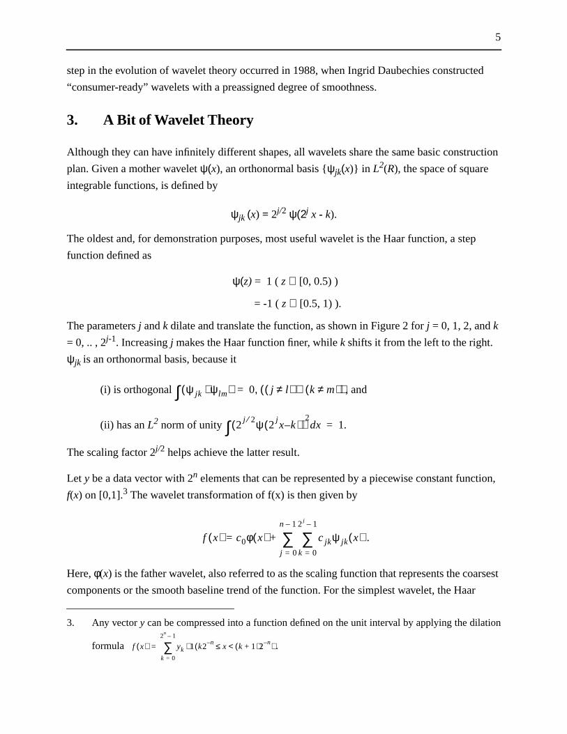
3. A Bit of Wavelet Theory

Although they can have infinitely different shapes, all wavelets share the same basic constru

plan. Given a mother waveletψ(x), an orthonormal basis {ψjk(x)} in L2(R), the space of square

integrable functions, is defined by

ψjk (x) = 2j/2 ψ(2j x - k).

The oldest and, for demonstration purposes, most useful wavelet is the Haar function, a ste

function defined as

ψ(z) = 1 (z ∈ [0, 0.5) )

= -1 (z ∈ [0.5, 1) ).

The parametersj andk dilate and translate the function, as shown in Figure 2 forj = 0, 1, 2, andk

= 0, .. , 2j-1. Increasingj makes the Haar function finer, whilek shifts it from the left to the right.

ψjk is an orthonormal basis, because it

(i) is orthogonal , and

(ii) has an L2 norm of unity

The scaling factor 2j/2 helps achieve the latter result.

Let y be a data vector with 2n elements that can be represented by a piecewise constant func

f(x) on [0,1].3 The wavelet transformation of f(x) is then given by

.

Here,φ(x) is the father wavelet, also referred to as the scaling function that represents the co

components or the smooth baseline trend of the function. For the simplest wavelet, the Haa

3. Any vectory can be compressed into a function defined on the unit interval by applying the dila

formula .

ψ jk ψ lm⋅( )∫ 0 j l≠( ) k m≠( )∨( ),=

2j 2⁄ ψ 2

jx k–( )( )

2xd∫ 1.=

f x( ) yk 1 k2n–

x k 1+( )2 n–<≤( )⋅k 0=

2n 1–

∑=

f x( ) c0φ x( ) cjkψ jk x( )k 0=

2 j 1–

∑j 0=

n 1–

∑+=

6

velet,

let are

s to

o zero.

ce.

e

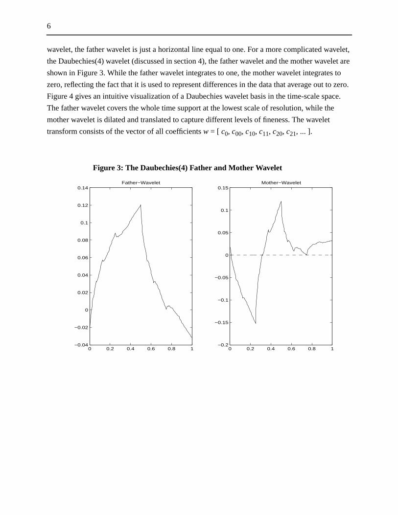
wavelet, the father wavelet is just a horizontal line equal to one. For a more complicated wa

the Daubechies(4) wavelet (discussed in section 4), the father wavelet and the mother wave

shown in Figure 3. While the father wavelet integrates to one, the mother wavelet integrate

zero, reflecting the fact that it is used to represent differences in the data that average out t

Figure 4 gives an intuitive visualization of a Daubechies wavelet basis in the time-scale spa

The father wavelet covers the whole time support at the lowest scale of resolution, while th

mother wavelet is dilated and translated to capture different levels of fineness. The wavelet

transform consists of the vector of all coefficientsw = [ c0, c00, c10, c11, c20, c21, ... ].

Figure 3: The Daubechies(4) Father and Mother Wavelet

0 0.2 0.4 0.6 0.8 1−0.04

−0.02

0

0.02

0.04

0.06

0.08

0.1

0.12

0.14Father−Wavelet

0 0.2 0.4 0.6 0.8 1−0.2

−0.15

−0.1

−0.05

0

0.05

0.1

0.15Mother−Wavelet

7

is

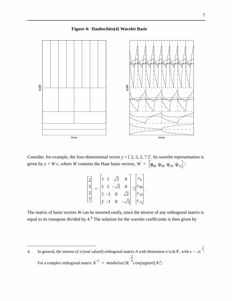
Figure 4: Daubechies(4) Wavelet Basis

Consider, for example, the four-dimensional vectory = [ 2, 5, 2, 7 ]’. Its wavelet representation is

given byy = W c,whereW contains the Haar basis vectors, :

.

The matrix of basis vectorsWcan be inverted easily, since the inverse of any orthogonal matrix

equal to its transpose divided by 4.4 The solution for the wavelet coefficients is then given by

4. In general, the inverse of a (real valued) orthogonal matrixA with dimensionn is , with .

For a complex orthogonal matrix .

time

scal

e

time

scal

e

W φ00 ψ00 ψ10 ψ11=

2

5

2

7

1 1 2 0

1 1 2– 0

1 1– 0 2

1 1– 0 2–

c0

c00

c10

c11

⋅=

αA' α A

2n---–

=

A1–

modulus A

2n---–

conjugate A( )'=

8

entity

our

plying

r [ 4

,

inally,

nal

tail

and

t four

.

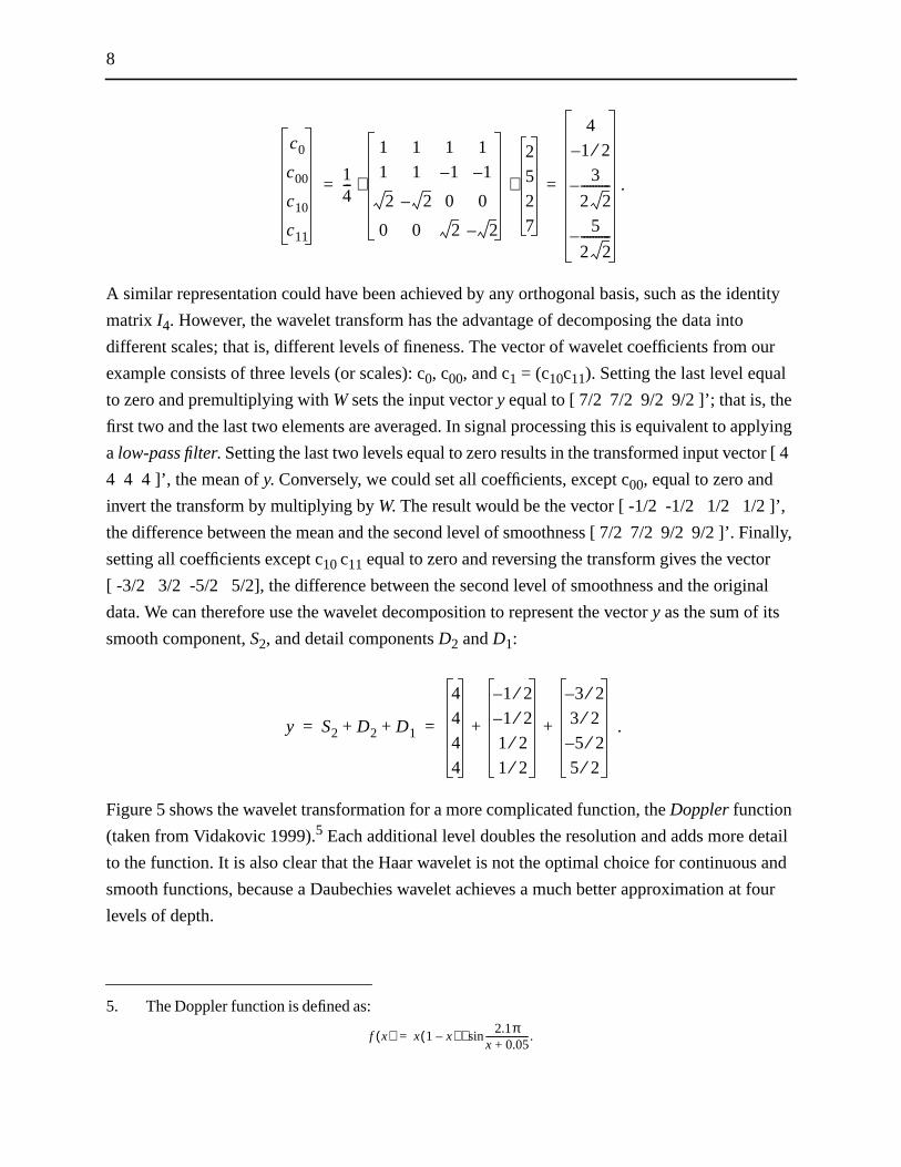
A similar representation could have been achieved by any orthogonal basis, such as the id

matrix I4. However, the wavelet transform has the advantage of decomposing the data into

different scales; that is, different levels of fineness. The vector of wavelet coefficients from

example consists of three levels (or scales): c0, c00, and c1 = (c10c11). Setting the last level equal

to zero and premultiplying withWsets the input vectory equal to [ 7/2 7/2 9/2 9/2 ]’; that is, the

first two and the last two elements are averaged. In signal processing this is equivalent to ap

a low-pass filter. Setting the last two levels equal to zero results in the transformed input vecto

4 4 4 ]’, the mean ofy. Conversely, we could set all coefficients, except c00, equal to zero and

invert the transform by multiplying byW. The result would be the vector [ -1/2 -1/2 1/2 1/2 ]’

the difference between the mean and the second level of smoothness [ 7/2 7/2 9/2 9/2 ]’. F

setting all coefficients except c10c11 equal to zero and reversing the transform gives the vector

[ -3/2 3/2 -5/2 5/2], the difference between the second level of smoothness and the origi

data. We can therefore use the wavelet decomposition to represent the vectory as the sum of its

smooth component,S2, and detail componentsD2 andD1:

.

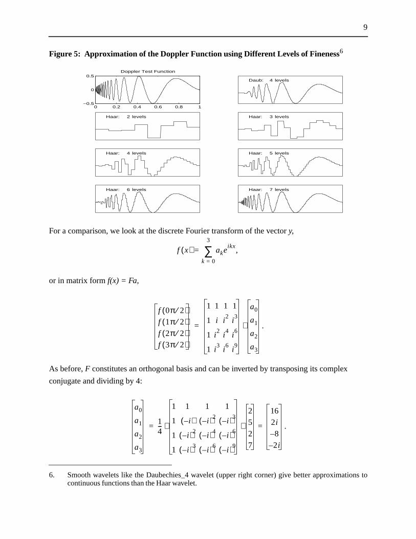
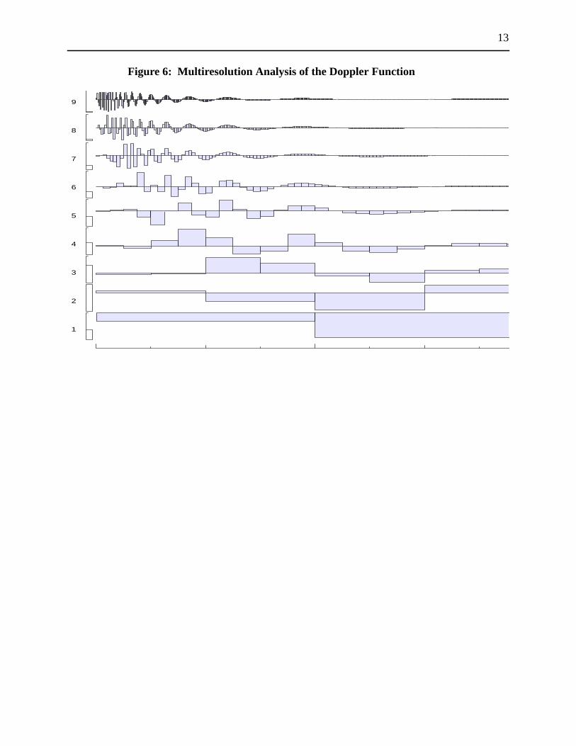
Figure 5 shows the wavelet transformation for a more complicated function, theDopplerfunction

(taken from Vidakovic 1999).5 Each additional level doubles the resolution and adds more de

to the function. It is also clear that the Haar wavelet is not the optimal choice for continuous

smooth functions, because a Daubechies wavelet achieves a much better approximation a

levels of depth.

5. The Doppler function is defined as:

c0

c00

c10

c11

14---

1 1 1 1

1 1 1– 1–

2 2– 0 0

0 0 2 2–

2

5

2

7

4

1 2⁄–

3

2 2----------–

5

2 2----------–

=⋅ ⋅=

y S2 D2 D1+ +

4

4

4

4

1– 2⁄1– 2⁄1 2⁄1 2⁄

3– 2⁄3 2⁄5– 2⁄5 2⁄

+ += =

f x( ) x 1 x–( ) 2.1πx 0.05+-------------------.sin⋅=

9

ons to

Figure 5: Approximation of the Doppler Function using Different Levels of Fineness6

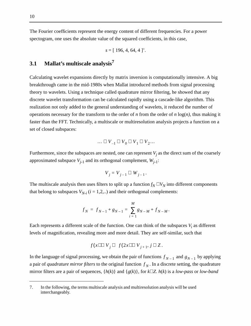
For a comparison, we look at the discrete Fourier transform of the vectory,

or in matrix formf(x) = Fa,

.

As before,F constitutes an orthogonal basis and can be inverted by transposing its complex

conjugate and dividing by 4:

.

6. Smooth wavelets like the Daubechies_4 wavelet (upper right corner) give better approximaticontinuous functions than the Haar wavelet.

0 0.2 0.4 0.6 0.8 1−0.5

0

0.5Doppler Test Function

Daub: 4 levels

Haar: 2 levels Haar: 3 levels

Haar: 4 levels Haar: 5 levels

Haar: 6 levels Haar: 7 levels

f x( ) akeikx

,k 0=

3

∑=

f 0π 2⁄( )f 1π 2⁄( )f 2π 2⁄( )f 3π 2⁄( )

1 1 1 1

1 i i2

i3

1 i2

i4

i6

1 i3

i6

i9

a0

a1

a2

a3

⋅=

a0

a1

a2

a3

14---

1 1 1 1

1 i–( ) i–( )2i–( )3

1 i–( )2i–( )4

i–( )6

1 i–( )3i–( )6

i–( )9

2

5

2

7

⋅

16

2i

8–

2i–

=⋅=

10

big

ing

his

of

on a

ying

re

The Fourier coefficients represent the energy content of different frequencies. For a power

spectogram, one uses the absolute value of the squared coefficients, in this case,

s = [ 196, 4, 64, 4 ]’.

3.1 Mallat’s multiscale analysis7

Calculating wavelet expansions directly by matrix inversion is computationally intensive. A

breakthrough came in the mid-1980s when Mallat introduced methods from signal process

theory to wavelets. Using a technique called quadrature mirror filtering, he showed that any

discrete wavelet transformation can be calculated rapidly using a cascade-like algorithm. T

realization not only added to the general understanding of wavelets, it reduced the number

operations necessary for the transform to the order ofn from the order ofn log(n), thus making it

faster than the FFT. Technically, a multiscale or multiresolution analysis projects a function

set of closed subspaces:

Furthermore, since the subspaces are nested, one can representVj as the direct sum of the coarsely

approximated subspaceVj-1 and its orthogonal complement,Wj-1:

.

The multiscale analysis then uses filters to split up a functionfN ∈VN into different components

that belong to subspacesVN-i (i = 1,2,..) and their orthogonal complements:

.

Each represents a different scale of the function. One can think of the subspacesVi as different

levels of magnification, revealing more and more detail. They are self-similar, such that

.

In the language of signal processing, we obtain the pair of functions and by appl

a pair ofquadrature mirror filtersto the original function . In a discrete setting, the quadratu

mirror filters are a pair of sequences, {h(k)} and {g(k)}, for k∈Z. h(k) is alow-pass or low-band

7. In the following, the terms multiscale analysis and multiresolution analysis will be usedinterchangeably.

… V 1– V0 V1 V2…⊂ ⊂ ⊂ ⊂

V j V j 1–= Wj 1–⊕

f N f N 1– gN 1– gN M– f N M–+i 1=

M

∑=+=

f x( ) V j f 2x( ) V j 1+ j Z∈,∈⇔∈

f N 1– gN 1–

f N

11

lters

the

es

g out

filter, whileg(k) is ahigh-pass or high-band filter. Intuitively, the low-pass filter makes the data

smoother and coarser, while the high-pass filter retains the detailed information. The two fi

are connected through the relation

.

Each wavelet has a scaling function, or father wavelet, , that spans the spaceV0 and can be

represented by a linear combination of functions from the next subspace,V1. Since the subspaces

are self-similar and nested, there exists a relationship between scaling functions of any two

neighbouring subspaces,Vj andVj+1. This relationship is called thescaling equation or dilation

equation and defines the filter coefficients:

.

In praxis, both filters are mappings froml(Z) to l(2Z); that is, they transform a vector withn

elements into two vectors withn/2 elements each, one of which contains the data smoothed by

low-pass filter, with the other containing the detail that was removed. Each wavelet can be

characterized by a finite set of filter coefficients derived from the scaling equation that relat

scaling functions of different subspaces,Vi, to each other. For the Haar wavelet, the filter

coefficients are

and .

Using the vector f(2) = [ 2 5 2 7 ]’ from our earlier example, the filtered vectors are given by

and .

f(1) is a weighted average of the first two and the second two entries off(2), respectively, where

the filter coefficients are used as weights. The same procedure is used forg(1), except that one of

the filter coefficients is negative, so that the weighted average is actually a difference, cuttin

detail fromf(1). It is convenient to use operatorsH andG to denote the filter relations applied to a

sequencea = {an}:

,

g n( ) 1–( )nh 1 n–( )=

φ

φ x( ) hk 2φ 2x k–( )k Z∈∑=

h 1( ) h 2( ) 1

2-------= = g 1( ) 1

2------- g 2( ) 1–

2-------=,=

f 1( ) 7

2------- 9

2-------= g 1( ) 3–

2------- 5–

2-------=

Ha( )k h n k–( )ann∑=

12

ked

is for

d

filters

a 2

.

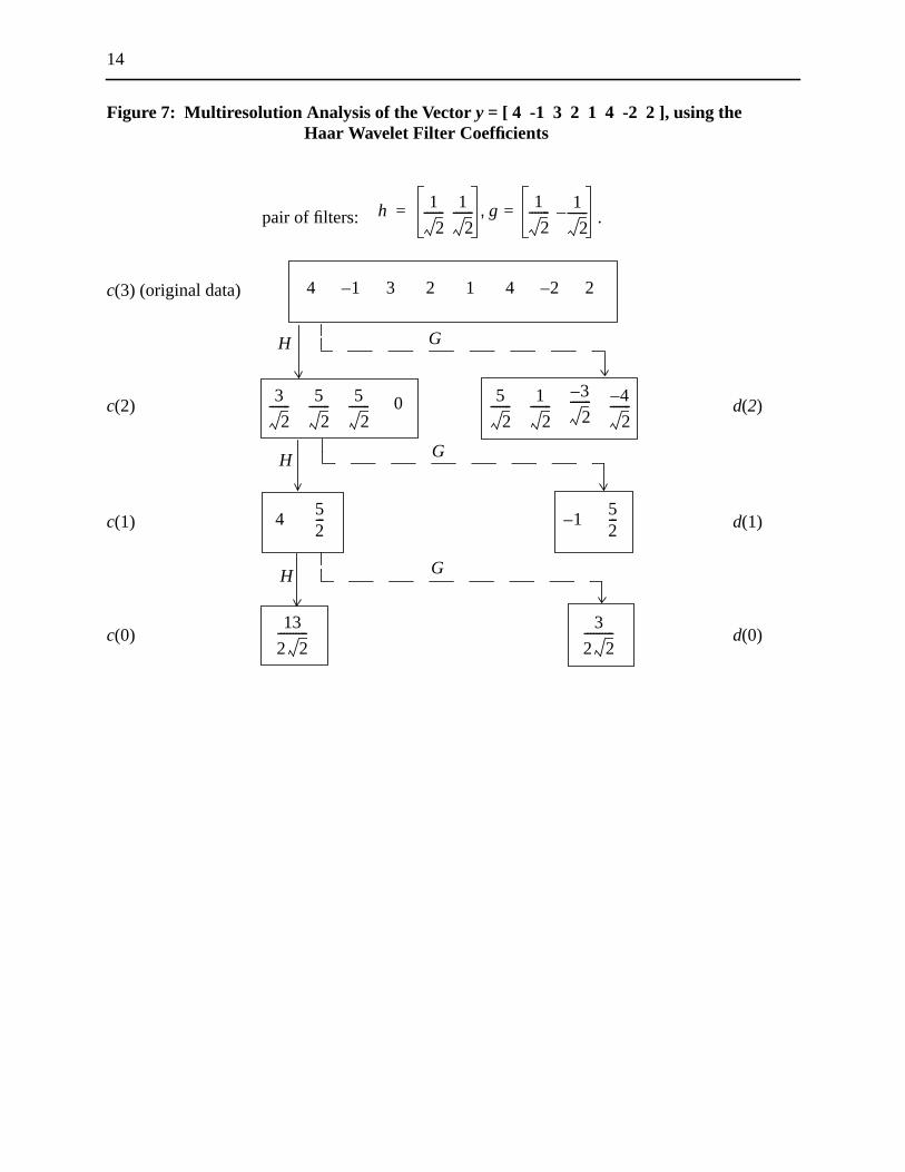
Let the original signal bec(n), a vector with 2n elements. Then,c(n-1) = H c(n) andd(n-1) = G c(n).

Applying the low-pass filter twice yieldsc(n-2) = H2 c(n) andd(n-2) = HG c(n). Using the

multiresolution analysis, the discrete wavelet transform of a sequencey = c(n) of length 2n is

another sequence of equal length, given by

w = [ d(n-1), d(n-2), ... ,d(1), d(0), c(0) ] = [ Gy, GHy, GH2y, ... ,GHn-1y, GHny, Hny ].

That is, the wavelet transform consists of all layers of detail, going from fine to coarse, stac

next to each other. Figure 6 shows the graphical interpretation of the multiresolution analys

the Doppler function from Figure 2 for a Haar wavelet transformation.

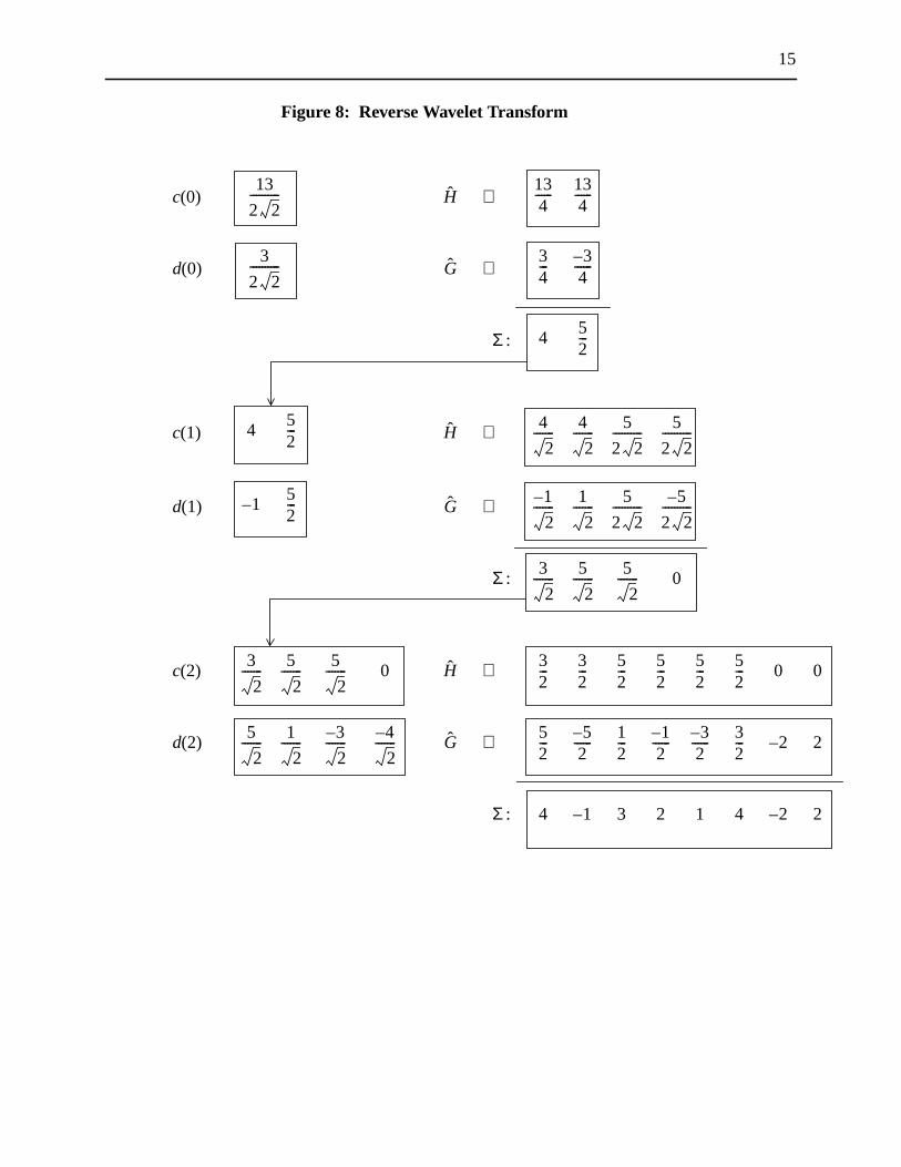
To invert the wavelet transform, an inverse filtering procedure is applied. The operators an

map a sequence froml(2Z) into l(Z), and each element is doubled and multiplied by the filter

coefficients. Consider, for example, applying the inverse low-pass and the inverse high-pass

to the vectorsf(1) andg(1):

.

Adding up the two expressions reproduces the initial vector,f(2).

Figures 7 and 8 give a detailed example of the decomposition and the inverse transform of3

vector using the Haar wavelet.

The wavelet transformation in multiresolution analysis form is then given byw = [ c(0),d(0),d(1),

d(2) ], or

.

To obtain the wavelet coefficients , one needs to multiplyw by , such that for the

equation ,c becomes

,

whereW is the matrix representing the Haar wavelet basis for eight dimensions.

Ga( )k g n k–( )ann∑=

H G

H f 1( ) 72--- 7

2--- 9

2--- 9

2--- Gg 1( ) 3–

2------ 3

2--- 5–

2------ 5

2---=,=

w 13

2 2---------- 3

2 2---------- 1–

52--- 5

2------- 1

2------- 3–

2------- 4–

2-------=

cjk 2N 2⁄–

y Wc=

c' 138------ 3

8--- 1

2 2----------–

5

4 2---------- 5

4--- 1

4--- 3–

4------ 1–=

13

Figure 6: Multiresolution Analysis of the Doppler Function

9

8

7

6

5

4

3

2

1

14

Figure 7: Multiresolution Analysis of the Vector y = [ 4 -1 3 2 1 4 -2 2 ],using theHaar Wavelet Filter Coefficients

pair of filters: .

c(3) (original data)

c(2) d(2)

c(1) d(1)

c(0) d(0)

h 1

2------- 1

2------- g 1

2------- 1

2-------–=,=

4 1– 3 2 1 4 2– 2

3

2------- 5

2------- 5

2------- 0 5

2------- 1

2-------

3–

2------- 4–

2-------

452--- 1–

52---

13

2 2---------- 3

2 2----------

H

H

H

G

G

G

15

0

2

2

Figure 8: Reverse Wavelet Transform

c(0) ⇒

d(0) ⇒

:

c(1) ⇒

d(1) ⇒

:

c(2) ⇒

d(2) ⇒

:

13

2 2---------- H

134------ 13

4------

3

2 2---------- G

34--- 3–

4------

Σ 452---

452--- H

4

2------- 4

2------- 5

2 2---------- 5

2 2----------

1–52--- G

1–

2------- 1

2------- 5

2 2---------- 5–

2 2----------

Σ 3

2------- 5

2------- 5

2------- 0

3

2------- 5

2------- 5

2------- 0 H

32--- 3

2--- 5

2--- 5

2--- 5

2--- 5

2--- 0

5

2------- 1

2------- 3–

2------- 4–

2------- G

52--- 5–

2------ 1

2--- 1–

2------ 3–

2------ 3

2--- 2–

Σ 4 1– 3 2 1 4 2–

16

pact

ents,

re 9

e

chies

.

4. Some Examples

We have already seen the Haar wavelet, but it has some serious limitations because of its

discontinuity. In Figure 4 we saw that a Daubechies wavelet is much more convenient for

approximating smooth functions. Daubechies wavelets were the first wavelet family with com

support and a preassigned degree of smoothness. They have an even number of filter elem

starting at 4. Wavelets within a family are usually denoted by the length of their filters. Figu

shows several specimens of the Daubechies family.

Figure 9: The Daubechies Family

Increasing the number of filter elements increases the support of the wavelet and makes th

wavelet smoother. The limiting case with two filter coefficients is the Haar wavelet. Daube

wavelets are asymmetric, a necessary property for compactly supported wavelets.8 It is, however,

8. In fact, the Haar wavelet is the only compactly supported orthonormal wavelet that is symmetric

0 1 2 3 4

−0.5

0

0.5

1

1.5

φ Daub4

0 1 2 3 4−2

0

2

ψ Daub4

0 2 4 6

−0.5

0

0.5

1

1.5

φ Daub6

0 2 4 6−2

0

2

ψ Daub6

0 2 4 6 8 10 12

−0.5

0

0.5

1

1.5

φ Daub12

0 2 4 6 8 10 12−2

0

2

ψ Daub12

0 5 10 15 20

−0.5

0

0.5

1

1.5

φ Daub20

0 5 10 15 20−2

0

2

ψ Daub20

17

d that

nother

y

by a

efined

s for

irable

tions;

possible to construct wavelets that are closely related cousins to the Daubechies family an

are more symmetric. These wavelets are called least asymmetric wavelets, or symmlets. A

family of wavelets, coiflets (Figure 10), are even less asymmetric than symmlets. Named b

Ingrid Daubechies after Ronald Coifman, these wavelets pay for their increased symmetry

larger support. Compared to Daubechies wavelets, their support is 3L-1 instead of 2L-1, whereL

denotes the number of vanishing moments.9

Figure 10: Coiflets and Biorthogonal Symmetric Wavelets

Biorthogonal wavelets relax the assumption of a single orthogonal basis. Instead, they are d

as a pair of mutually orthogonal bases, neither of which is orthogonal. This relaxation allow

the construction of compactly supported symmetric wavelets. This property is especially des

in image processing. Biorthogonal wavelets have primary and dual scaling and wavelet func

9. A wavelet hasN(>=2) vanishing moments if ,n = 0, 1, ...,N-1.ψ xnψ x( ) xd∫ 0=

0 5 10 15

−0.5

0

0.5

1

1.5

φ Coif18

0 5 10 15−2

0

2

ψ Coif18

0 2 4 6 8

−2

0

2

4

φ1 Biorth

3.3

0 2 4 6−4

−2

0

2

4

ψ1 Biorth

3.3

0 2 4 6 8−1

0

1

2

φ2 Biorth

3.3

0 2 4 6−2

0

2

ψ2 Biorth

3.3

0 2 4 6

−0.5

0

0.5

1

1.5

φ Coif6

0 2 4−2

0

2

ψ Coif6

18

oiflets

ince

main.

ian

olute

an example is shown in the last two rows in Figure 10 for BS_2.2. Figure 11 shows some c

and biorthogonal wavelets with different numbers of filter coefficients.

The following subsections describe some of the most useful ways in which wavelets can be

applied in practice.

4.1 Filtering

One of the main applications of frequency analysis concerns the filtering of noisy signals. S

white noise is uncorrelated at all lags and leads, it is distributed evenly over the frequency do

Graph (a) in Figure 12 shows a digital impulse in the time domain that is covered by Gauss

white noise (Graph (b)). Graphs (c) and (d) show the power spectral density (normalized abs

value of the squared Fourier transform) and the wavelet transformation of the noisy signal.

Figure 11: Coiflets and Biorthogonal Symmetric Wavelets

0 5 10 15

−0.5

0

0.5

1

1.5

φ Coif18

0 5 10 15−2

0

2

ψ Coif18

0 2 4 6 8

−2

0

2

4

φ1 Biorth

3.3

0 2 4 6−4

−2

0

2

4

ψ1 Biorth

3.3

0 2 4 6 8−1

0

1

2

φ2 Biorth

3.3

0 2 4 6−2

0

2

ψ2 Biorth

3.3

0 2 4 6

−0.5

0

0.5

1

1.5

φ Coif6

0 2 4−2

0

2

ψ Coif6

19

idth

ilities

the

rior

e is

Gibbs

in the

eason

ting

one

ising

sting

To filter out the white noise, all coefficients in the frequency domain below a certain bandw

are set equal to zero. This process is called a “hard” thresholding rule. (Several other possib

for thresholding are shown in Figure 13.) The filtered series are then transformed back into

time domain. A comparison between graphs (e) and (f) in Figure 12 shows the clearly supe

performance of the inverse wavelet transform to restore the original signal. The performanc

superior because the Fourier transform relies on a large number of layers to suppress the

effect (that is, the over- and undershooting at discontinuities), because its basis is non-local

time domain and some of the higher layers are rubbed out in the filtering process. Another r

is that the Haar wavelet, which was used in this example, is particularly useful in approxima

step functions like the rectangular pulse signal.

Figure 12: Filtering

The method of using thresholding rules to filter data was developed by Donoho and Johnst

(1994) and it is called wavelet shrinkage, or WaveShrink. Its main advantage is that the de-no

is carried out without smoothing out sharp structures such as spikes and cusps. One intere

application is in seismology, where researchers observe the water levels of wells to predict

0 0.2 0.4 0.6 0.8 1

0

0.5

1

(a) Pure Signal

amp

0 0.2 0.4 0.6 0.8 1

0

0.5

1

(b) Noisy Signal

amp

0 0.2 0.4 0.6 0.8 1−10

−5

0

5

10(d) Wavelet Decomposition

0 0.2 0.4 0.6 0.8 1

0

0.5

1

(e) Inverse Fourier Transform Using a Filter

0 0.2 0.4 0.6 0.8 1

0

0.5

1

(f) Inverse Wavelet Transform Using a Filter

amp

100 200 300 400 5000

5

10(c) Power Spectral Density

20

e

re 14,

ed

r

Since

we

earthquakes. Wavelets can filter out the noise without removing the spikes that characteriz

changes in water levels prior to earthquakes.

Figure 13: Different Thresholding Rules

4.2 Separation of frequency levels

In another application, two sine functions with different frequencies are added up (see Figu

first row). To filter each component of the combined signal, we look at how much energy is

contained in each scale of the wavelet transform. This can be done by adding up the squar

coefficients in each scale to get a scalogram. The scalogram can be compared to the powe

spectral plot in Fourier analysis.

In the scalogram, we can observe two spikes: one at the third level and one at the sixth level.

slow-moving, low-frequency components are represented by wavelets with larger support,

−10 −5 0 5 10−10

−5

0

5

10hard

−10 −5 0 5 10−10

−5

0

5

10soft

−10 −5 0 5 10−10

−5

0

5

10firm

−10 −5 0 5 10−10

−5

0

5

10garrote

−10 −5 0 5 10−10

−5

0

5

10hard

−10 −5 0 5 10−10

−5

0

5

10soft

−10 −5 0 5 10−10

−5

0

5

10firm

−10 −5 0 5 10−10

−5

0

5

10garrote

21

six

first

four

rse

ince

aling

cales.

an

ations.

the

conjecture that level three represents the wavelet transform for function one, and that level

represents the wavelet transform for function two. To filter out function one, we keep only the

four levels and pad the rest of the wavelet transform with zeros. Then we take the inverse

transform. Conversely, we keep levels five to nine for the second function and pad the first

levels with zeros. The last two graphs in Figure 14 show the filtered series given by the inve

transformations. In this particular case, a Fourier transform would be much more efficient, s

the underlying functions are purely periodic. But wavelets are more useful when we are de

with non-periodic data. Many economic data are likely generated as aggregates of different s

Separating these scales and analyzing them individually provides interesting insights and c

improve the forecasting accuracy of the aggregate series. Section 5 describes some applic

Figure 14: Separation of Frequency Levels

4.3 Disbalancing of energy

This is a relatively abstract concept, but it has very interesting implications. By referring to

energy of a signal or data vector, we mean its -norm:

.

0 200 400 600 800 1000−5

−4

−3

−2

−1

0

1

2

3

4

5low frequency

0 200 400 600 800 1000−5

−4

−3

−2

−1

0

1

2

3

4

5high frequency

0 200 400 600 800 1000−5

−4

−3

−2

−1

0

1

2

3

4

5combined signal

0 2 4 6 8 100

200

400

600

800

1000

1200

1400

1600

1800

2000scalogram

cut

0 200 400 600 800 1000−5

−4

−3

−2

−1

0

1

2

3

4

5inv. transform (high freq.)

0 200 400 600 800 1000−5

−4

−3

−2

−1

0

1

2

3

4

5inv. transform (low freq.)

L2

y2

y2i

i∑=

22

nergy.

s and

ct that

om the

ntury

s. A

ifts

of the

torage,

Since the wavelet transform is an orthonormal operation, it preserves the total amount of e

It distorts its distribution, however, making it more unequal. Figure 15 shows the time serie

the wavelet transform of a unit root process. The lower scales hold most of the energy, a fa

makes intuitive sense, because the unit root process is characterized by lasting deviations fr

current mean. The second row of Figure 15 shows the Lorentz curves for the two series.

Figure 15: Disbalancing of Energy

The Lorentz curve was initially developed by economists at the beginning of the twentieth ce

to study the distribution of income. It graphs the cumulative distribution against the quantile

45-degree line would represent a completely homogeneous data set, whereas the curve sh

lower as inequality rises. The Lorentz curve of the wavelet transform is so close to the edge

graph that it can hardly be seen.

Why do we want to disbalance the energy of a signal? There are several reasons. For data s

this means that the signal can be well described by a fairly short sequence. In statistics

200 400 600 800 1000

0

20

40

60

80

Unit Root Process

200 400 600 800 1000−80

−60

−40

−20

0

20

40

60

80Wavelet Transform

0 0.2 0.4 0.6 0.8 10

0.2

0.4

0.6

0.8

1Lorentz−curve of Time Series

0 0.2 0.4 0.6 0.8 10

0.2

0.4

0.6

0.8

1Lorentz−curve of wavelet transform

0 200 400 600 800 1000−20

0

20

40

60

80

100Unit Root Process

0 200 400 600 800 1000−1000

−500

0

500

1000

1500

2000Wavelet Transform

0 0.2 0.4 0.6 0.8 10

0.1

0.2

0.3

0.4

0.5

0.6

0.7

0.8

0.9

1Lorentz Curve of Time Series

0 0.2 0.4 0.6 0.8 10

0.1

0.2

0.3

0.4

0.5

0.6

0.7

0.8

0.9

1Lorentz Curve of Wavelet Transform

23

ies are

ales.

le

del as

f

over

ws a

series

he

ree

disbalancing the energy can increase the variance between different distributions, thereby

increasing the power of a test.

4.4 Whitening of correlated signals

The hierarchical construction of wavelets means that non-stationary components of time ser

absorbed by the lower scales, while non-lasting disturbances are captured by the higher sc

This leads to a phenomenon that Vidakovic (1999) calls the whitening property. The examp

shown in Figure 16 uses an integrated autoregressive moving average (ARIMA) (2,1,1) mo

a data-generating process, a realization of which is illustrated in the first graph. This kind o

process contains a unit root; therefore, the autocorrelation function shows almost no decay

20 periods. On the other hand, the autocorrelation of the differenced ARMA(2,1) model sho

drop after two periods, as predicted by the Box and Jenkins model selection criterion.

Figure 16: Whitening of Correlated Signals

The wavelet transform decomposes the time series into log2 (T) scales. In our case, the time

has 512 observations, so that we have nine scales. The last six graphs in Figure 16 show t

autocorrelation functions of the six highest layers of the original ARIMA series (the bottom th

0 100 200 300 400 500−40

−20

0

20

40

60

80

ARIMA(2,1,1)

0 5 10 15 20−1

−0.5

0

0.5

1

ACFARIMA

0 5 10 15 20−1

−0.5

0

0.5

1

ACFARMA

0 5 10 15 20−1

−0.5

0

0.5

1

ACFw9

0 5 10 15 20−1

−0.5

0

0.5

1

ACFw8

0 5 10 15 20−1

−0.5

0

0.5

1

ACFw7

0 5 10 15 20−1

−0.5

0

0.5

1

ACFw6

0 5 10 15 20−1

−0.5

0

0.5

1

ACFw5

0 5 10 15 20−1

−0.5

0

0.5

1

ACFw4

24

lation

. This

other

h. All

lso be

msey

tionary

a time

write:

ctrum

to

ale-to-

lly all

oints

.

ekly,

do not

e

layers have four or less elements, not enough information to compute the autocorrelation

functions).

Note that the ninth scale looks almost like a white noise signal, while scales six and four, in

particular, show clear signs of autocorrelation at all included lags. Moreover, these autocorre

functions are oscillating, indicating a presence of a mean reverting autoregressive process

mean reverting behaviour at the higher scales is a result of the absorbtion of the trend and

non-stationary components by the lower scales.

5. Applications for Economists

This section discusses some fields where wavelets have been applied to economic researc

applications are related to econometrics; however, it is quite possible that wavelets might a

applied in one way or another directly to theoretical research. Parts of this survey follow Ra

(1996), who the reader is referred to for a more detailed treatment of some of the topics.

5.1 Frequency domain analysis

A general result, called the spectral representation theorem, states that any covariance-sta

process has a representation in both the time domain and the frequency domain. In terms of

series that has a moving average representation, using the Fourier transformation, we can

.

One of the first applications of wavelets to time-series analysis was the estimation of the spe

density for stationary Gaussian processes (Gao 1993).10 Neumann (1996) extends the analysis

non-Gaussian processes. Given the ability of wavelets to break down a time series on a sc

scale basis, each scale corresponding to a range of frequencies, they can be used in virtua

applications that were previously based on Fourier analysis. However, as Priestley (1996) p

out, there is only an intuitive and very indirect connection between frequency and the scale

The Fourier transform is based on periodic functions in the time domain, thus capturing we

monthly, or yearly cycles. However, many economic phenomena, such as business cycles,

follow this strict periodicity, favouring the more flexible wavelet approach. Conway and Fram

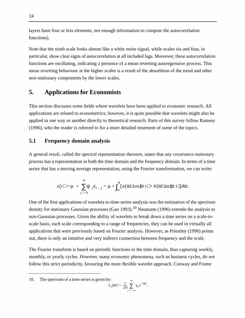
10. The spectrum of a time series is given by:.

x t( ) µ ψ jεt j– µ a ω( ) ωt( ) b ω( ) ωt( )sin+cos[ ] ωd0

π∫+=

j 0=

∞

∑+=

Sx ω( ) 12π------ γ je

i ω j–

j ∞–=

∞

∑=

25

tent of

ers.

a

re

mator

e

based

rs are

e of

is

elet

nging

r time.

ard &

w

s

(2000), for example, use both Fourier and wavelet techniques to analyze the frequency con

output gaps generated by different methods ranging from structural VARs to mechanical filt

5.2 Non-stationarity and complex functions

Nason and von Sachs (1999) and von Sachs and MacGibbon (2000) focus on signals with

possibly time-changing probability distribution; that is, locally stationary processes whose

moments exhibit slow change. Quasi-stationarity can be defined as a situation in which mo

observations per unit period of time would lead to locally asymptotic convergence of the

estimators. The authors suggest the use of a local minimum absolute deviation (MAD) esti

to estimate the variance of the wavelet coefficients within the quasi-stationary levels. An

important consequence is the suitability of wavelet estimators for generalized autoregressiv

conditional heteroscedasticity (GARCH) processes.

Following the seminal paper of Donoho and Johnstone (1994), a whole set of estimators is

on the notion of wavelet shrinkage, filtering noise using thresholding rules. These estimato

discussed in detail in Vidakovic (1999, ch. 6). Gao (1997) applies this technique for the cas

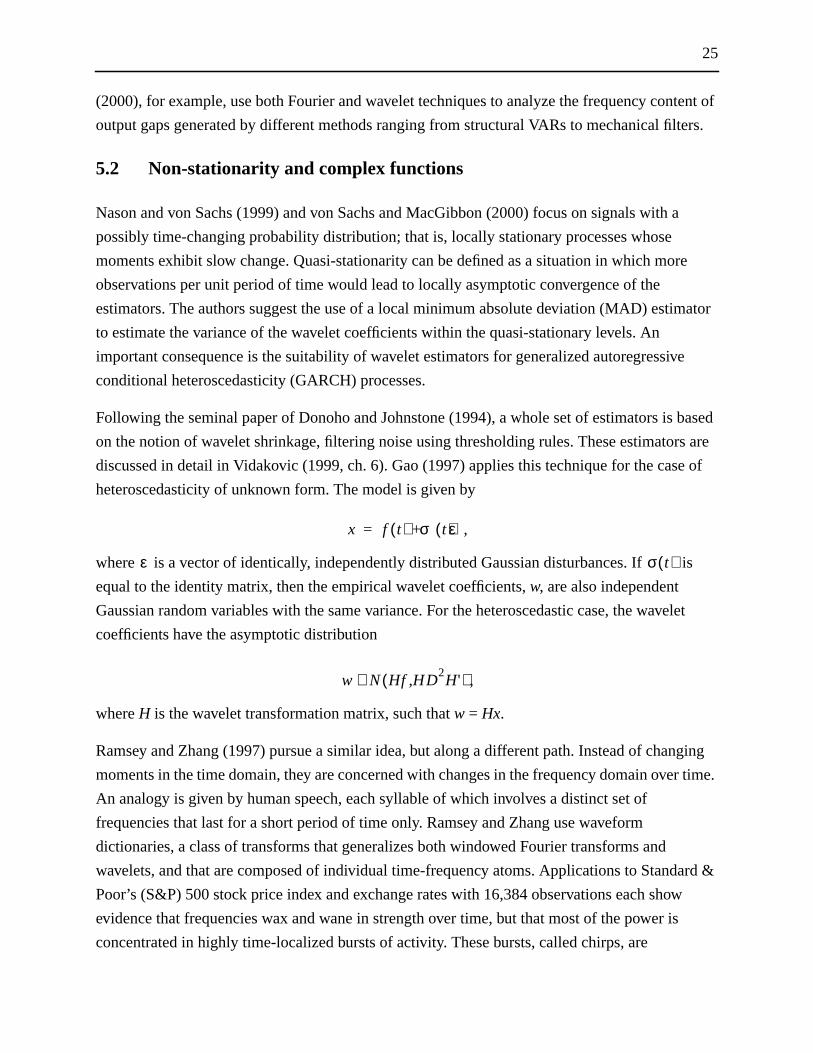
heteroscedasticity of unknown form. The model is given by

,

where is a vector of identically, independently distributed Gaussian disturbances. If

equal to the identity matrix, then the empirical wavelet coefficients,w, are also independent

Gaussian random variables with the same variance. For the heteroscedastic case, the wav

coefficients have the asymptotic distribution

,

whereH is the wavelet transformation matrix, such thatw = Hx.

Ramsey and Zhang (1997) pursue a similar idea, but along a different path. Instead of cha

moments in the time domain, they are concerned with changes in the frequency domain ove

An analogy is given by human speech, each syllable of which involves a distinct set of

frequencies that last for a short period of time only. Ramsey and Zhang use waveform

dictionaries, a class of transforms that generalizes both windowed Fourier transforms and

wavelets, and that are composed of individual time-frequency atoms. Applications to Stand

Poor’s (S&P) 500 stock price index and exchange rates with 16,384 observations each sho

evidence that frequencies wax and wane in strength over time, but that most of the power i

concentrated in highly time-localized bursts of activity. These bursts, called chirps, are

x f t( ) σ t( )ε+=

ε σ t( )

w N Hf HD2H',( )∼

26

at

of

small

has

ears,

ays at

g-

ess

Hurst

(1999)

ption

ed is

the log

s a

mean

ero.

characterized by a rapid buildup of amplitude and rapid oscillation. The authors conclude th

transmission of information is not a swift and effortless process, but that there are periods

adjustment represented by the chirps. Although the data can be represented by a relatively

number of atoms (about 100), there seems to be no way of forecasting the chirps.

5.3 Long-memory processes

The importance of differentiating between stationary I(0) and non-stationary I(1) processes

long been one of the focal points in theoretical and applied time-series analysis. In recent y

the attention of researchers has shifted towards fractionally integrated I(d) processes, that lie in

the grey area between the two sharp-edged alternatives of I(0) and I(1). Specifically, whend lies

between 0 and 0.5, the process still has a finite variance, but its autocovariance function dec

a much slower rate than that of a stationary ARMA process. Such processes are called lon

memory processes. Whend lies between 0.5 and 1, the variance becomes infinite, but the proc

still returns to its long-run equilibrium. The study of long-memory processes dates back to

(1951) and has been applied to a number of economic time series in recent years. Jensen

cites a wide range of applications, including real GDP, interest rates, stock market returns, o

prices, and exchange rates.

A fractionally integrated process, I(d), can be defined by

,

where is white noise or follows an ARMA process.

Because long-memory processes have a very dense covariance matrix, direct maximum-

likelihood estimation is not feasible for large data sets. Instead, the estimator most often us

based on a nonparametric approach, which regresses the log values of the periodogram on

Fourier frequencies to estimated (Geweke and Porter-Hudak (GPH) 1983).

McCoy and Walden (1996) find a log-linear relationship between the wavelet coefficients’

variance and its scale and develop a maximum-likelihood estimator. Jensen (1999) develop

simpler, ordinary least-squares (OLS) estimator that is based on the observation that for a

zero I(d) process, |d| < 0.5, the wavelet coefficients, (for scale (dilation)j and translationk),

are asymptotically normally distributed with mean zero and variance as j goes to z

Taking logs, we can estimated using the linear relationship

,

1 L–( )dx t( ) ε t( )=

ε t( )

djk

σ22

2 jd–

R j( ) σ2d 2

2 jln–ln=ln

27

OLS

nte-

ve

ts to

e

rt-run

llat’s

ifferent

ney

ictory

to

let

ng-run

ul: (i)

ded or

r

thors

riods,

se and

d.

-

e with

ll be a

where R(j) is the sample estimate of the covariance in each scale. The wavelet estimators (

and maximum likelihood) have a higher small-sample bias than the GPH estimator, but Mo

Carlo experiments show that they have a mean-squared error that is about six times lower.

Mandelbrot and van Ness (1968) find self-similarities in fractional Brownian motions that ha

been observed in physical sciences as well as in financial time series. The ability of wavele

dissect data into different scales makes it possible to detect these self-similar phenomena.

Vidakovic (1999, p. 14, pp. 292) gives an overview of some of the related literature.

5.4 Time-scale decompositions: the relationship between money and incom

It has long been recognized that economic decision-making is dependent on the time scale

involved, and economists emphasize the importance of discerning between long-run and sho

behaviour. Wavelets offer the possibility of going beyond this simplifying dichotomy by

decomposing a time series into several layers of orthogonal sequences of scales using Ma

multiscale analysis. These scales can then be analyzed individually and compared across d

series.

Ramsey and Lampart (1998a) use this method to examine the relationship between the mo

supply (M1 and M2) and output. The related literature has produced ambiguous and contrad

results regarding the Granger causality of the two variables, a fact that has been attributed

structural breaks and possible non-linearities. Ramsey and Lampart offer the alternative

explanation that the contradictions may well be explained by the existence of overlaying

timescale-structured relationships. To unmask these relationships, the authors use a wave

transform to decompose the time series into a low-frequency base scale that captures the lo

trend and six higher-frequency levels. Here, two more interesting facets of wavelets are usef

since the base scale includes any non-stationary components, the data need not be detren

differenced; and (ii), the nonparametric nature of wavelets takes care of potential non-linea

relationships without losing detail. Applying causality tests to the decomposed series, the au

find that, at the lowest timescales, income Granger causes money, but at business-cycle pe

money Granger causes income. At the highest scales, the Granger causality goes in both

directions, suggesting some form of feedback mechanism. These results make intuitive sen

also explain why there are ambiguous causal relationships when timescales are aggregate

A second important finding is that the causal relationship between different variables is non

stationary even along individual scales, since the two series are moving into and out of phas

each other. To explain these phase shifts and to differentiate them from structural breaks wi

further challenge for theoretical and applied researchers.

28

lope

cales

each

ty used

l and

is

ator

ntly,

earch;

d

e

first

ral

eural

he

IMA

ughly

quency

n, the

n be

In a companion paper, Ramsey and Lampart (1998b) analyze the relationship between

consumption and income at different timescales. As predicted by theory, they find that the s

coefficient relating consumption and income declines with scale.

5.5 Forecasting

Ariño (1998) and Ariño, Pedro, and Vidakovic (1995) describe a very simple approach for

forecasting time series using wavelets. First, the time series is decomposed into different s

using the wavelet transform. Ariño shows that, by adding up the squared coefficients within

level, one can measure the energy content of each scale, similar to the power spectral densi

in Fourier analysis. Using the properties of the multiscale analysis, the time series is then

decomposed into two separate series. Each individual is then fitted using an ARIMA mode

the aggregate forecast is obtained by adding up the individual forecasts. Ariño shows that h

forecasts are preferable to a standard Box and Jenkins approach, but does not discuss the

distributional properties of his forecast. A useful first step would be to test the wavelet estim

against other estimators using a Monte Carlo simulation.

A second field of application is the use of wavelets in connection with neural networks. Rece

wavelet networks have gained wide acceptance in physics, engineering, and biological res

however, their use for forecasting economic time series has been limited so far. Aussem an

Murtagh (1997) and Aussem, Campbell, and Murtagh (1998) can find an improvement in th

prediction of sunspots and the S&P 500 index. Similar to Ariño’s approach, the time series is

decomposed into different scales. Each scale is then used to train a dynamic recurrent neu

network and the individual forecasts are added up to obtain the combined forecast. Since n

networks need a lot of variation to extract information, only scales with a relatively high

frequency can be used.

The main benefit of wavelets in forecasting appears to be their ability to reveal features in t

individual scales that are dampened by the overlapping scales. It is therefore easier for AR

models or neural networks to extract periodic information in the individual scales.

6. Conclusions

Wavelets open a large, unexplored territory to applied economic researchers that can be ro

decomposed into three areas. The first area covers research that is related to Fourier and fre

analysis. While the Fourier transform maps from the time domain into the frequency domai

wavelet transform decomposes a time series into a set of different scales, each of which ca

29

ures of

n in

ss the

arate

isions

is

el or

ment

tions.

t more

such

) and

ut

his

99)

d

loosely associated with a range of frequencies. The second area exploits several useful feat

wavelets to improve statistical inference. These features are the ability to localize a functio

both time and scale, to deal with non-linear and non-stationary environments, and to compre

energy content of a signal. The third area directly addresses the dissection of data into sep

layers or scales. From a theoretical viewpoint, this is of special interest, since economic dec

and actions take place at different timescales that overlap. For forecasting purposes, there

evidence that the individual scales provide the forecasting mechanism (e.g., an ARIMA mod

an artificial neural network) with more detailed information than the aggregate signal.

All three areas leave ample room for future research. For example, evidence for the improve

of forecasts by decomposing the time series is largely anecdotal and based on individual

examples. A next step would be to calculate small sample properties and asymptotic distribu

The fact that wavelet transforms disbalance the energy of a signal could be used to construc

powerful tests; for example, for structural breaks or unit roots. A lot of statistical techniques,

as wavelet shrinkage estimators, that have been worked out and applied in biometrics and

engineering could be applied to econometrics.

7. How to Get Started

There are a couple of easy and intuitive primers on wavelet theory; for example, Graps (1995

Vidakovic and Mueller (1994). Vidakovic (1999) provides a more complete and technical, b

accessible, treatment.

Most researchers use either MatLab or S-Plus to model wavelets. Both platforms offer

commercial wavelet toolboxes as well as free add-ons. The examples and graphs used in t

survey were made using Ojanen’s (1998) WaveKit toolbox for MatLab (www.math.rutgers.edu/

~ojanen/wavekit). Another free MatLab toolbox is WaveLab, developed by Donoho et al. (19

at Stanford (www-stat.stanford.edu/~wavelab). WaveLab has a very large set of commands an

includes datasets and educational add-ons.

A good link to the newest developments and new publications in wavelet research is

www.wavelet.org.

30

an-

inty,

ecom-

s-

urier0/06.

//

is-

ub-

ime

ni-

Bibliography

Ariño, M.A. 1998. “Forecasting Time Series via Discrete Wavelet Transform.” Unpublished muscript.

Ariño, M.A., M. Pedro, and B. Vidakovic. 1995. “Wavelet Scalograms and Their ApplicationEconomic Time Series.” Institute of Statistics and Decision Sciences, Duke UniversiDiscussion Paper No. 94–13.

Aussem, A., J. Campbell, and F. Murtagh. 1998. “Wavelet-Based Feature Extraction and Dposition Strategies for Financial Forecasting.”Journal of Computational Intelligence inFinance (March/April): 5–12.

Aussem, A. and F. Murtagh. 1997. “Combining Neural Network Forecasts on Wavelet-Tranformed Time Series.”Connection Science 9(1): 113–21.

Conway, P. and D. Frame. 2000. “A Spectral Analysis of New Zealand Output Gaps Using Foand Wavelet Techniques.” Reserve Bank of New Zealand Discussion Paper No. 200

Daubechies, I. 1988. “Orthonormal Bases of Compactly Supported Wavelets.”Communicationson Pure and Applied Mathematics 41: 909–96.

———. 1992.Ten Lectures on Wavelets. Society for Industrial and Applied Mathematics.

Davison, R., W.C. Labys, and J.-B. Lesourd. 1998. “Wavelet Analysis of Commodity PriceBehavior.”Journal of Computational Economics 11: 103–28.

Donoho, D.L. and I.M. Johnstone. 1994. “Ideal Spatial Adaptation via Wavelet Shrinkage.”Bio-metrica 81: 425–55.

Donoho, D.L. et al. 1999.WaveLab. Stanford University, Department of Statistics. <URL: http:www-stat.stanford.edu/~wavelab>.

Gao, H.-Y. 1993. “Wavelet Estimation of Spectral Densities in Time Series Analysis.” PhD Dsertation, Department of Statistics, University of California, Berkeley.

———. 1997. “Wavelet Shrinkage Estimates for Heteroscedastic Regression Models.” Unplished manuscript, MathSoft, Inc.

Geweke, J. and S. Porter-Hudak. 1983. “The Estimation and Application of Long Memory TSeries Models.”Journal of Time Series Analysis 4: 221–38.

Graps, A. 1995. “An Introduction to Wavelets.”IEEE Computational Science and Engineering2(2): 50–61.

Hernandez, E. and G.L. Weiss. 1996. “A First Course on Wavelets.” CRC, Boca Raton.

Hong, Y. 1999. “One-Sided Testing for ARCH Effect Using Wavelets.” PhD thesis, Cornell Uversity.

Hurst, H.E. 1951. “Long-Term Storage Capacity of Reservoirs.”Transactions of the AmericanSociety of Civil Engineers 116: 770–99.

31

tor of

Treat-

nta-

and

em-

Sci-

tion-

ial

cale

lets:

iour

Dic-

Jensen, M.J. 1999. “Using Wavelets to Obtain a Consistent Ordinary Least Squares Estimathe Long-Memory Parameter.”Journal of Forecasting 18: 17–32.

———. 2000. “An Alternative Maximum Likelihood Estimator of Long-Memory Processesusing Compactly Supported Wavelets.”Journal of Economic Dynamics & Control 24:361–87.

Lapenta, E.S., S.M. Abecasis, and C.A. Heras. 2000. “Discrete Wavelet Transforms for thement of Financial Time Series.” Unpublished manuscript. <URL: http://www.sarabe1@infovia.com.ar>.

Mallat, S. 1989. “A Theory for Multiresolution Signal Decomposition: The Wavelet Represetion.” IEEE Transactions on Pattern Analysis and Machine Intelligence 11: 674–93.

Mallat, S. and Z. Zhang. 1993. “Matching Pursuits with Time-Frequency Dictionaries.”IEEETransactions on Signal Processing (December): Vol. 41, No. 12.

Mandelbrot, B.B. and J.W. van Ness. 1968. “Fractional Brownian Motions, Fractional NoisesApplications.”SIAM Review 10(4): 422–37.

McCoy, E.J. and A.T. Walden. 1996. “Wavelet Analysis and Synthesis of Stationary Long-Mory Processes.”Journal of Computational and Graphical Statistics 5(1): 26–56.

Nason, G.P. and R. von Sachs. 1999. “Wavelets in Time Series Analysis.”Philosophical Transac-tions of the Royal Society London, Series A: Mathematical, Physical and Engineeringences 357: 2511–26.

Neumann, M.H. 1996. “Spectral Density Estimation via Nonlinear Wavelet Methods for Staary Non-Gaussian Time Series.”Journal of Time Series Analysis 17: 601–33.

Ojanen, H. 1998.WAVEKIT: A Wavelet Toolbox for Matlab. Department of Mathematics, RutgersUniversity.

Percival, D.B. and A.T. Walden. 2000.Wavelet Methods for Time Series Analysis. New York:Cambridge University Press.

Priestley, M. 1996. “Wavelets and Time-Dependent Spectral Analysis.”Journal of Time SeriesAnalysis 17: 85–103.

Ramsey, J.B. 1996. “The Contribution of Wavelets to the Analysis of Economic and FinancData.” Unpublished manuscript.

Ramsey, J.B. and C. Lampart. 1998a. “Decomposition of Economic Relationships by TimesUsing Wavelets.”Macroeconomic Dynamics 2(1): 49–71.

———. 1998b. “The Decomposition of Economic Relationships by Time Scale using WaveExpenditure and Income.”Studies in Nonlinear Dynamics and Econometrics 3(1): 23–42.

Ramsey, J.B., D. Usikov, and G.M. Zaslavskiy. 1995. “An Analysis of U.S. Stock Price BehavUsing Wavelets.”Fractals 3(2): 377–89.

Ramsey, J.B. and Z. Zhang. 1997. “The Analysis of Foreign Exchange Data using Waveformtionaries.”Journal of Empirical Finance 4: 341–72.

32

resh-

velet

ta-

ion,

Sachs, R. von and B. MacGibbon. 2000. “Non-Parametric Curve Estimation by Wavelet Tholding with Locally Stationary Errors.”Scandinavian Journal of Statistics 27: 475–99.

Sachs, R. von and M. Neumann. 2000. “A Wavelet-Based Test for Stationarity.”Journal of TimeSeries Analysis 21: 597–613.

Spokoiny, V.G. 1996. “Adaptive Hypothesis Testing using Wavelets.”The Annals of Statistics24(6): 2477–98.

Strang, G. 1993. “Wavelet Transforms versus Fourier Transforms.”Bulletin (new series) of theAmerican Mathematical Society 28(2): 288–305.

Strichartz, R.S. 1993. “How to Make Wavelets.”American Mathematical Monthly 100: 539–56.

Tkacz, G. 2000. “Estimating the Fractional Order of Integration of Interest Rates Using a WaOLS Estimator.”Studies in Nonlinear Dynamics and Econometrics 5: 19–32.

Vidakovic, B. 1999.Statistical Modeling by Wavelets. New York: John Wiley and Sons.

Vidakovic, B. and P. Mueller. 1994. “Wavelets for Kids, A Tutorial Introduction.” Institute of Stistics and Decision Sciences, Duke University, Discussion Paper No. 95–21.

Whitcher, B.J. 1998. “Assessing Nonstationary Time Series Using Wavelets.” PhD dissertatDepartment of Statistics, University of Washington.

Bank of Canada Working PapersDocuments de travail de la Banque du Canada

Working papers are generally published in the language of the author, with an abstract in both officiallanguages.Les documents de travail sont publiés généralement dans la langue utilisée par les auteurs; ils sontcependant précédés d’un résumé bilingue.

Copies and a complete list of working papers are available from:Pour obtenir des exemplaires et une liste complète des documents de travail, prière de s’adresser à:

Publications Distribution, Bank of Canada Diffusion des publications, Banque du Canada234 Wellington Street, Ottawa, Ontario K1A 0G9 234, rue Wellington, Ottawa (Ontario) K1A 0G9E-mail: publications@bankofcanada.ca Adresse électronique : publications@banqueducanada.caWeb site: http://www.bankofcanada.ca Site Web : http://www.banqueducanada.ca

20022002-2 Asset Allocation Using Extreme Value Theory Y. Bensalah

2002-1 Taylor Rules in the Quarterly Projection Model J. Armour, B. Fung, and D. Maclean

20012001-27 The Monetary Transmission Mechanism at the Sectoral Level J. Farès and G. Srour

2001-26 An Estimated Canadian DSGE Model withNominal and Real Rigidities A. Dib

2001-25 New Phillips Curve with Alternative Marginal Cost Measuresfor Canada, the United States, and the Euro Area E. Gagnon and H. Khan

2001-24 Price-Level versus Inflation Targeting in a Small Open Economy G. Srour

2001-23 Modelling Mortgage Rate Changes with aSmooth Transition Error-Correction Model Y. Liu

2001-22 On Inflation and the Persistence of Shocks to Output M. Kichian and R. Luger

2001-21 A Consistent Bootstrap Test for Conditional DensityFunctions with Time-Dependent Data F. Li and G. Tkacz

2001-20 The Resolution of International Financial Crises:Private Finance and Public Funds A. Haldane and M. Kruger

2001-19 Employment Effects of Restructuring in the PublicSector in North America P. Fenton, I. Ip, and G. Wright

2001-18 Evaluating Factor Models: An Application toForecasting Inflation in Canada M.-A. Gosselin and G. Tkacz

2001-17 Why Do Central Banks Smooth Interest Rates? G. Srour

2001-16 Implications of Uncertainty about Long-RunInflation and the Price Level G. Stuber

2001-15 Affine Term-Structure Models: Theory and Implementation D.J. Bolder

2001-14 L’effet de la richesse sur la consommation aux États-Unis Y. Desnoyers