by ari glezerl and donald coles2 - california...

J . Fluid Mech. (1990), vol. 211, p p . 243-283 Printed in Great Britain

243

An experimental study of a turbulent vortex ring By ARI GLEZERl AND D O N A L D COLES2

Department of Aerospace and Mechanical Engineering, University of Arizona, Tucson, AZ 8572 1 , USA

California Institute of Technology, Pasadena, CA 91125, USA

(Received 18 July 1987 and in revised form 12 July 1989)

A turbulent vortex ring having a relatively thin core is formed in water by a momentary jet discharge from an orifice in a submerged plate. The necessary impulse is provided by a pressurized reservoir and is controlled by a fast programmable solenoid valve. The main aim of the research is to verify the similarity properties of the mean flow, as defined by ensemble averaging, and to find the distribution of mean vorticity, turbulent energy, and other quantities in the appropriate non-steady similarity coordinates. The velocity field of the vortex is measured for numerous realizations with the aid of a two-channel tracking laser-Doppler velocimeter. The problem of dispersion in the trajectories of the individual rings is overcome by development of a signature-recognition technique in two variables. It is found that the turbulence intensity is largest near the vortex core and that a t least the radial component is not negligible in the near wake. The slow growth of the ring structure is controlled by a slight excess of entrainment over de-entrainment. An important inference is that the growth process and the process of turbulence production probably involve secondary vortices wrapped around the core in azimuthal planes.

1. Introduction The research reported here is a contribution to the subject of coherent structure

in turbulent flow. The structure chosen for experimental study is the turbulent vortex ring, which does not have an extensive literature. Most of the literature on single non-buoyant vortex rings is concerned with laminar rings, with emphasis on the formation process and on an elegant instability in which azimuthal waves appear on the vortex core. Quantitative data a t various locations downstream of the orifice of a vortex generator have previously been obtained using either hot-wire (HWA) or laser-Doppler (LDA) anemometry, mostly for laminar flow, by Akhmetov & Kisarov (1966, HWA), Johnson (1970, HWA), Sullivan, Widnall & Ezekiel (1973, LDA), Sallet & Widmayer (1974, HWA), Kovasznay, Fujita & Lee (1974, HWA), Didden (1977, LDA), and Maxworthy (1977, LDA). Whenever the flow in question is turbulent, serious problems with dispersion in the trajectories of individual rings are either reported explicitly or can be deduced from the nature of the published data. Except for data on celerity and growth rate and a few estimates of the ratio of core diameter to ring diameter, no systematic quantitative information about turbulent structure was obtained in any of the experiments just cited.

The non-steady similarity formulation for the turbulent vortex ring is based on the invariance of the hydrodynamic impulse for an unbounded flow, and has been derived by a number of investigators (e.g. Johnson 1970). The concept of similarity, however, has not been fully exploited to resolve important structural questions

244 A . Glezer and D. Coles

regarding entrainment and turbulent production. The apparatus and inst,rum- ent8ation developed for this purpose during the research are described briefly in $92 and 3. A more detailed account of the apparatus can be found in the thesis by Glezer (1981), and some optical and mechanical specifications for the laser-Doppler instrumentation can be found in Glezcr & Coles (1982).

For present purposes, a vortex ring can be defined as an axially symmetric, spheroidal volume of fluid whose internal mean vorticity lies entirely in the azimuthal direction. This vorticity (better, the ratio vorticity/radius) may be more or less uniformly distributed, in which case the structure is often called a vortex puff (the Hill spherical vortex, although inviscid, falls in this category) ; or the vorticity may be mostly concentrated in a thin toroidal core, in which case t'he term vortex ring is more accurate. The distinction between vortex puff and vortex ring can be neglected for many purposes, including the discussion of similarity for the special case of turbulent flow in $4.

As mentioned above, a formidable obstacle to experimental study of the turbulent vort,ex ring is dispersion in the path followed by successive rings as they travel from the generating device to the point of observation. Any description of the flow in tcrms of ensemble-averaged quantities is therefore likcly to lack resolution and to misrepresent the physical processes actually involved. Section 5 describes the elaborate methods which had to be developed to overcome this problem of dispersion.

From t,he beginning, the object of the research was to determine mean particle paths by exploiting the fact that the property of similarity reduces the Lagrangian particle-path equations to an autonomous system. The spirit of the analysis in $6, and some of the procedures, follow the precedents set by Woodward (1959) for the thermal, by Turner (1964) for a model problem involving the Hill spherical vortex, and by Cant,well, Coles & Dimotakis (1978) for the turbulent spot, in a laminar boundary layer. The t,opological structure of the turbulent vortex ring was found, as expected, to consist of two saddle points on the axis, together with a ring focus. However, special measures described in 5 7 were required to determine mean particle paths that are in agreement with an independent estimate of the net entrainment based on a streamline pattern relative to the moving vortex. In an attempt to resolve this question by different mcans, some flow visualization was carried out using fluorescent dye and high-speed motion-picture photography. The entrainment process is found to involve substantial transfer of fluid into or out of the spheroidal ring structure at different azimuthal positions on the mean interface. These observations are described in $8.

Finally, $9 is a gcneral discussion of the experimental findings and some of their implications.

2. The experimental apparatus The experiments were carried out in water contained in a glass tank 1 m on a side.

Vortex rings were generated at a circular orifice in a ceiling plate suspended just below the free water surface, as indicated schematically in figure 1. The rings moved vertically downward in the tank. The flow could be illuminated and viewed directly from the four sides and could also be viewed from below with the aid of a mirror in the tank.

The impulse necessary to produce the vortex rings camc from a momentary discharge of water from the pressurized reservoir shown abovc the tank in figure 1 .

A n experimental study of a turbulent vortex ring 245

( Accumulator Pressure

regulator

Diaphragm

Solenoid valve

FIGURE 1. Schematic diagram (not to scale) showing the vortex-ring generator used in the present experiments.

The flow out of the reservoir was controlled by a fast annular-outlet solenoid valve? energized by a solid-state relay. The low-mass internal poppet had a total travel of less than 1 mm and could open or close in an interval as short as 6 ms, with repeatability of 0.1 ms under computer control. The stainless-steel reservoir could be pressurized by nitrogen up to 2100 kPa (300 psi). The gas pressure was held constant by a pressure regulator selected for smooth operation a t low flow rates. An accumulator connected to the upper end of the reservoir prevented pressure drops in excess of about 7 kPa (1 psi) during discharge.

The solenoid-valve outlet opened into the top of a cylindrical chamber containing a light-weight plastic piston. The cylindrical space below the piston was open to the tank. For a given reservoir pressure, cylinder length, and piston starting position, the valve time T, could easily be adjusted to within a fraction of a millisecond so that the piston stopped when its bottom surface was flush with the plane wall within 0.1 mm. Thus, a t the beginning of the generation process, the geometric configuration was a simple cylindrical cavity in a plane wall. At the end of the generation process, the wall became an uninterrupted plane. This scheme eliminated any strong secondary flow at the end of the stroke, and it standardized some egects of the image system for the vortex ring during and especially after formation. The piston motion can be described by a simple top-hat velocity program U, = U,[H(t) -H( t - To)]. The piston velocity V, could be varied between 10 and 130 cm/s, and the respective acceleration

t Two of these valves were made available to us through the courtesy of Dr Raymond Goldstein of NASA’s Jet Propulsion Laboratory, Pasadena, California.


FIGURE 2. Photographs, using dye for flow visualization, of (a) a laminar vortex ring at r,/v x 7500, (b) a turbulent vortex ring at T,/v x 27000.

and deceleration a t the beginning and end of the stroke were typically 35 cm/s/ms at moderate reservoir pressures. After each experiment, the piston was restored to its original starting position with the aid of a small pump. Seeding for laser-Doppler measurements was automatic, because the fluid drawn into the cylindrical cavity was seeded fluid from the glass tank.

The lip of the cylinder in the vortex generator was fitted with nine small orifices for dye injection (figure 1) so that water entering the cavity from below could be mixed with dye solution for the purpose of flow visualization. Typical photographs of a laminar and a turbulent ring are shown in figure 2.

3. The experiment Some optical features of the laser-Doppler velocimeter (LDV) designed and

constructed as part of this research have been described elsewhere (Glezer &, Coles 1982). Beam splitting and frequency shifting were accomplished by a pair of overlapping radial phase gratings driven by hysteresis-synchronous motors. Bias

An experimental study of a turbulent vortex ring 247

frequencies during the present experiment were set a t 195 kHz for the axial component of velocity and a t 1755 kHz for the radial component. The sensitivity for both components was 1.299 kHz per cm/s, and the bias frequencies were modulated by Doppler frequencies of, a t most, f 150 kHz. A single silicon avalanche photodiode detector was followed by a transimpedance amplifier. The two data channels were separated electronically a t the amplifier output by band-pass filters which also rejected cross-talk frequencies of 780 kHz and 975 kHz. The signal-tracking circuits incorporated a digital phase-locked loop configured for fast response to a step input. There was no difficulty in tracking signals near the orifice or near the core of the vortex ring for velocity changes as large as 400 m/s/s (i.e. an equivalent acceleration of 40 times gravity), and the velocity field could be resolved to within 1 mm/s. The tank was seeded with styrene divinylbenzene particles of 5.7pm diameter a t a concentration of about 20 000 particles/cm3. On the average, perhaps 10 particles were present in the LDV test volume at any instant.

Two-channel LDV measurements were made of the velocity field associated with one particular turbulent vortex ring. The operating conditions for the vortex generator were chosen to produce a ring for which dye visualization showed a well- defined and reasonably repeatable flow structure. The kinematic viscosity v during the experiment was 0.010 cmz/s (water a t 20 "C). The orifice/piston diameter was

Do = 1.905 f 0.002 em and the piston stroke was

Lo = 6.52f0.01 em.

Hence, Lo/Do = 3.42. The reservoir pressure was 2100 kPa. The valve was open for a period

To = 51.0f0.1 ms

and the nominal piston velocity was therefore

U, = Lo/% = 127.8f0.4cm/s.

An elementary representation of the programmed discharge of fluid, which forms a vortex ring, is a uniform cylindrical-slug model. I n this model, a cylindrical volume of fluid moves a t a constant velocity U, for a time T, through a circular orifice of diameter Do. Based on this model, the nominal impulse (taken to be the momentum associated with the discharge) was

I / p = ~ X D : Lo U, = 2374 f 15 cm4/s

and the nominal circulation, made dimensionless with the kinematic viscosity, was

ro/ v = T, /2v = 41 650 f 300. The motion is conveniently described in a cylindrical polar coordinate system

(2, r , 6), with corresponding velocity components (u, v, w). The axial coordinate x increases downward, with the origin in the plane of the orifice. Velocity measurements were made for an ensemble of 100 vortices at each of numerous probe stations. The data reported here were obtained during an axial traverse along the axis of symmetry from x = 0.1 em to x = 50.0 em and a radial traverse normal to the horizontal optical axis a t x = 35.0 cm.

A 10 MHz crystal-controlled pulse train was used as a master time base for the measurements. Division by lo4 generated a 1 kHz pulse train, or clock, whose primary function was to regulate the sampling interval of 1 ms. The clock signal also controlled the grating rotation, which was thus precisely synchronized with data


U

r

L I I I I I I I I I I I 400 600 800 1000 1200 1400

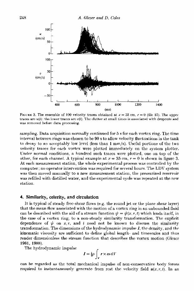
(ms) FICURE 3. The ensemble of 100 velocity traces obtained at z = 35 em. r = 0 (file 15). The upper traces are u( t ) ; the lower traces are v( t ) . The clutter at small times is associated with dropouts and was removed before data processing.

sampling. Data acquisition normally continued for 5 s for each vortex ring. The time interval between rings was chosen to be 90 s to allow velocity fluctuations in the tank to decay to an acceptably low level (less than 1 mm/s). Useful portions of the two velocity traces for each vortex were plotted immediately on the system plotter. Under normal conditions, a hundred such traces were plotted, one on top of the other, for each channel. A typical example a t x = 35 cm, r = 0 is shown in figure 3. At each measurement station, the whole experimental process was controlled by the computer ; no operator intervention was required for several hours. The LDV system was then moved manually to a new measurement station, the pressurized reservoir was refilled with distilled water, and the experimental cycle was repeated a t the new station.

4. Similarity, celerity, and circulation It is typical of steady free-shear flows (e.g. the round jet or the plane shear layer)

that the mean flow associated with the motion of a vortex ring in an unbounded fluid can be described with the aid of a stream function @ = @(x, r , t ) which lends itself, in the case of a vortex ring, to a non-steady similarity transformation. The explicit dependence of $ on x , r , and t need not be known to discuss the similarity transformation. The dimensions of the hydrodynamic impulse I , the density, and the kinematic viscosity are sufficient to define global length- and timescales and thus render dimensionless the stream function that describes the vortex motion (Glezer 1981, 1988).

I = + p J v r x o d V

can be regarded as the total mechanical impulse of non-conservative body forces required to instantaneously generate from rest the velocity field u(x,r,t). In an

The hydrodynamic impulse


unbounded viscous fluid, the hydrodynamic impulse is an invariant of the motion. The vortex interacts briefly with the generator during its formation and as a result may lose some of its initial impulse. For a given fluid, the invariance of I once the vortex ring moves away from the generator makes the hydrodynamic impulse the main dimensional parameter of the flow and allows various vortex ring flows to be ordered according to their strength.

If the flow is laminar, all three independent variables are required to describe the motion. If the flow is turbulent, its dependence on the kinematic viscosity may be neglected ; hence, the similarity transformation for a turbulent vortex ring must fail far from the vortex core because the induced velocity vanishes a t infinity. Maxworthy (1974) has noted that hydrodynamic impulse is continuously lost from the vortex bubble (which includes the core) to the wake and hence concluded that for the vortex bubble a similarity transformation based on the invariance of the impulse is not possible. The present stream-function formulation for unsteady axisymmetric flow in an unbounded domain applies to both the vortex bubble and its wake. This formulation becomes approximate only where viscous effects are important. As will be shown below, the applicability of the similarity transformation is strongly supported by the data.

During the experiment, the origin for x was taken in the plane of the orifice and the origin for t was taken a t the beginning of the generation process. Before the resulting data can be interpreted in similarity variables, however, i t is necessary to define and determine an apparent origin (x,,t,) in space and time.

The non-steady similarity formulation for the stream function $ for a turbulent vortex ring (e.g. Glezer 1981) is

where I is nominal initial impulse or increment of momentum.

stream function can be written In explicit dimensionless form, with the apparent origin taken into account, the

where

s = $ - (t-t,) i = S(C,?/l), ty

The velocity components are defined by u = (l /r)a$/ar, v = -(l /r)a$/ax. In similarity variables, these are

The essence of these relationships is a set of simple rules. For any point which is

( a ) r - (x-x,) , (b ) ( ~ 1 . ~ ) ~ - (!-to), ( c ) u-5 - (t-to)* - (x-xn). The rules just stated have been recognized and applied in several previous studies

of the turbulent puff or the turbulent vortex ring. For example, motion pictures or probe measurements were used with rule ( a ) to verify the property of conical growth,

fixed in similarity coordinates


and thus to determine xo, by Grigg & Stewart (1963), Johnson (1970), and Kovasznay et al. (1973). Kovasznay et al. also invoked rule (c), taking u to be either the overall celerity? or the peak mean velocity on the axis of symmetry. Once the origin for x is known, rule ( b ) allows the origin for t to be determined, as in the papers by Grigg & Stewart (1963), Richards (1965), and Johnson (1970). Roughly speaking, for a vortex puff, both xo and to tend to be positive; i.e. the origin in x is downstream of the orifice, and the origin in time is later than the actual beginning of the motion. For a vortex ring with a thin core, the opposite is usually true, as was first noted by Turner (1957).

In principle, the rules just outlined can readily be used to determine xo and to for the present measurements by using data obtained on the axis of symmetry. However, severe problems with dispersion caused the actual calculation to become quite elaborate. The circulation for a turbulent vortex ring decreases continuously, like (t-t,)-$, during the lifetime of the ring (see (6) below). This decay process is manifested by irregular shedding of vorticity (i.e. smoke or dye) into the wake, as shown in figure 2 ( 6 ) and in similar photographs published, for example, by Northrup (1912)) Johnson (1970), Maxworthy (1974), Sallet & Widmayer (1974), Oshima, Kovasznay & Oshima (1977)) and Schneider (1980). Because the shedding is irregular and unsymmetric, there is substantial dispersion of the trajectories of individual vortex rings in both space and time. The problem is apparent in figure 3, which displays the ensemble of raw traces for axial and radial velocities for 100 vortex rings observed at x = 35 cm, r = 0. The peak in the axial velocity in the upper part of the figure shows considerable scatter, both in amplitude and in arrival time. The radial velocity often shows the N-shaped profile that is characteristic of flow off the axis of symmetry. Resolution of this problem of dispersion was a major preoccupation throughout the present research. The need was to eliminate from a given ensemble the traces showing anomalous behaviour without biasing or prejudicing the mean properties of the remaining data. A procedure was devised for this purpose, after considerable development, and applied to the various data files on the axis of symmetry for the purpose of determining the parameters xo and to. Only an outline of the data processing is given here; details can be found in Glezer (1981).

A preliminary step was data preparation. For each of the 100 vortex rings in a file, a time window was set to capture the non-trivial part of the signal (in both channels) from the passing vortex. The LDV bias frequency for each channel was subtracted. Grating noise was removed, using amplitude and phase information computed from a synchronized data record maintained for this purpose. Occasional small gaps caused by momentary dropout of the Doppler signal during data acquisition were filled in by linear interpolation. The data were crudely low-pass filtered; i.e. each data point was replaced by the mean of five symmetrically located points. The peak axial velocity up and the corresponding arrival time t , for each u-trace were determined by the computer. The time window was set to a standard length (191 ms; hereinafter referred to as the standard time interval) and centred on t , for each trace.

As part of the data processing, vortex rings judged to be unfit on the basis of early or late arrival time, large radial velocity, or atypical axial velocity were discarded during several ite,rations until the population at each measurement station on the axis of symmetry was reduced to approximately 30 vortex rings. When the values

t Although Sallet & Widmayer (1974) did not discuss the question of similarity, this method using celerity could have been applied to their data.

An experimental study of a turbulent vortex ring

0.4

0.3 <u>,i

25 1

-

-

I I I I 1 I

0 10 20 30 40 50

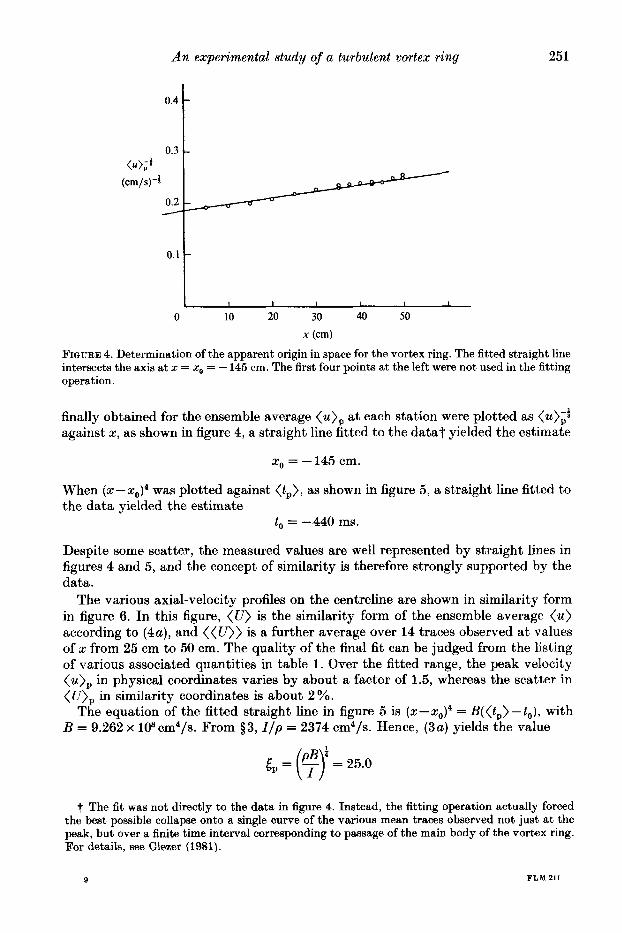
x (cm) FIQURE 4. Determination of the apparent origin in space for the vortex ring. The fitted straight line intersects the axis at x = xo = - 145 cm. The first four points at the left were not used in the fitting operation.

finally obtained for the ensemble average (u), at each station were plotted as (u);i against x , as shown in figure 4, a straight line fitted to the data? yielded the estimate

xo = - 145 cm.

When ( X - X ~ ) ~ was plotted against ( t , ) , as shown in figure 5, a straight line fitted to the data yielded the estimate

to = -440 ms.

Despite some scatter, the measured values are well represented by straight lines in figures 4 and 5, and the concept of similarity is therefore strongly supported by the data.

The various axial-velocity profiles on the centreline are shown in similarity form in figure 6. In this figure, (U) is the similarity form of the ensemble average ( u ) according to (4a), and ((U)) is a further average over 14 traces observed at values of x from 25 cm to 50 cm. The quality of the final fit can be judged from the listing of various associated quantities in table 1. Over the fitted range, the peak velocity (u) , in physical coordinates varies by about a factor of 1.5, whereas the scatter in ( U ) , in similarity coordinates is about 2 %.

The equation of the fitted straight line in figure 5 is ( X - X ~ ) ~ = B(( tp ) - to ) , with B = 9.262 x 108 cm4/s. From 53, I / p = 2374 cm4/s. Hence, (3a ) yields the value

pB 4 E, = (r) = 25.0

t The fit was not directly to the data in figure 4. Instead, the fitting operation actually forced the best possible collapse onto a single curve of the various mean traces observed not just a t the peak, but over a finite time interval corresponding to passage of the main body of the vortex ring. For details, me Glezer (1981).

9 FLM 211


0 200 400 600 800 1000 1200

(f,> (ms)

FIQURE 5. Determination of the apparent origin in time for the vortex ring. The fitted straight line intersects the axis a t t = to = -440 ms. The first four points a t the left were not used in the fitting operation.

24.0 24.8 25.6 5

FIGURE 6. Superposition in similarity variables of 14 mean axial-velocity profiles on the axis of symmetry at various values of 2. The ordinate is normalized to have a peak value of unity for the overall average profile ( ( V ( 5 ) ) ) . The origin for the final global fit is at xo = - 145 cm, to = -440 ms.

for the location of the peak in figure 6. According to (3a) in differential form, the locus of peak axial velocity on the axis of symmetry has the celerity

= 39.7cm/s c , , = ( $ ) = B

p 4(x--2d3 at 2 = 35 cm (or x-xo = 180 cm). The celerity in similarity coordinates follows from (4a) and from the expressions just obtained;

( t - to) : = = 6.25.

The final quantity that was determined from the centreline data is the circulation r, defined by a contour integral as indicated in figure 7. At any fixed time, three of the boundaries of the contour can be placed far enough from the ring (whose far field is essentially an axisymmetric dipole) so that their contribution to the contour


(W, File x 0,) (u), -

number (cm) (ms) (cm/s) ((WP) 5 25 461 96.7 1.010 6 25 461 96.8 1.012 7 30 572 85.6 0.985 8 35 690 76.5 0.966

15 35 695 80.5 0.999 9 37.5 757 75.3 0.984

10 40 824 72.8 0.987 11 42.5 896 73.1 1.025 42 42.5 895 74.1 1.026 61 42.5 891 70.0 0.979 12 45 967 71.8 1.030 13 47.5 1044 64.5 1.008 14 50 1121 59.8 0.968 33 50 1120 64.7 1.022

TABLE 1. Peak u-velocity and its arrival time on axis of symmetry

FIGURE 7. Contour of circulation integral.

integral is negligible. The contribution of the remaining boundary, i.e. the axis of symmetry, is

roo r= J (u)dx.

0

The data stations on the axis of symmetry were not spaced closely enough to define the function (~(2)) accurately. However, by writing ( 5 ) in similarity form with the aid of (3a) and (4a), the integral over x a t fixed t can be interpreted as an integral over t a t fixed x. Thus,

The quantity G , defined by

is evidently a proper constant of the motion. We note in passing that, for a viscous vortex ring, the invariance of the hydrodynamic impulse implies that TO2 = constant, where D is the diameter of the ring (Saffman 1970). Because the diameter of a turbulent vortex ring increases like (t-to):, i t follows that its circulation decreases like (t-to)-a. At x = 35 cm, the function ( U ( 5 ) ) is defined experimentally

9.2

254 A . Glexer and D . Coles

for times up to about 4.8 s (6 = 17.065); the corresponding experimental contribution to the integral in (7) is 7.275. For larger times, the data were extrapolated to 6 = 0 by the formula ( U ) = (0.02245)2.5, which is a good fit to the experimental values in the far wake (1.9 < t < 4.8 8 ) . No particular significance is attached to the exponent 2.5. The further contribution for this range is 0.439, so that finally

G = Jom(U)dt = 7.71.

5. Dispersion In the procedure just described, effects of dispersion were suppressed by retaining

only the 30 % or so of realizations that showed acceptably small excursions from the mean in both the axial and radial components of velocity. When the off-axis data were examined, it was immediately obvious that the radial dispersion in ring trajectory was substantially larger than the radial distance between probe stations. Furthermore, the various rings differed in their displacements normal to the traverse line, in their circulations, and in their small-scale internal details. All of these differences had to be reconciled before the mean flow could be established, which is to say before turbulent fluctuations could be evaluated as excursions from the mean. At the same time, turbulent fluctuations interfered with the reconciliation a t every stage. The main data-processing effort therefore went into schemes designed to finesse the problem of turbulent fluctuations until they could finally be accurately defined.

The first and most important step was to develop a signature-recognition scheme in two variables as a basis for ordering the various realizations. The variables of the scheme are defined in figure 8, which shows, for two typical realizations, the two measured components of velocity as functions of time during passage of the main ring structure. Figure 8 ( a ) represents a slice through the ring between the axis and the core, and figure 8 ( b ) represents a slice near the outer edge of the core. For each such pair of signals, two characteristic quantities were defined that took into account the different natures of the u- and v-traces. One quantity, u,, was the axial velocity a t the time corresponding to location of the probe in the plane of the thin vortex core. This velocity was usually, but not always, a global extreme value, as in figure 8(a). Because the decision was not one that could be confidently delegated to the computer, the value of u, was established manually for each u-trace by displaying the data on a cathode-ray-tube screen, moving a cursor to the proper position on the trace (hence the subscript c), and reading from the discrete data array the values for u, and for the corresponding time t, (tP for the data files on the axis of symmetry). The other quantity, up, was the difference vm,,-vmin. This difference was defined to be positive if vmax preceded vmin in time, and was unambiguously determined by the computer.

Figure 9(a ) is a plot of the two signature parameters u, and up, one against the other. All of the 1800 realizations observed a t 2 = 35 cm are included. Note that neither the radial position of the probe nor the arrival time t, plays any role in construction of the figure. The scatter is appreciable, but the density of data points varies in a reasonably smooth manner, and a definite pattern can be discerned, Several features of figure 9 (a) are worth comment :

(a) There is a gap in up at the right, near the u,-axis, that indicates the magnitude of turbulent fluctuations in v near the axis of symmetry of the vortex ring. There are no traces in this region for which the peak-to-peak excursion in v is less than about


FIGURE 8. Typical experimental velocity traces for two realizations, showing definition of characteristic magnitudes u, and vD. Time interval is 191 ms.

9 cm/s. Note also that a given point lies above (below) the horizontal axis if the positive (negative) extremum in v occurs first in time. Thus, there might be considerable movement of data points in both directions across the axis if the values of up were recalculated for heavily smoothed rather than raw traces. Our decision was not to attempt smoothing in this context because of the risk of smearing the data near the core and in the vicinity oft,.

( b ) The small gap near the origin in the main sequence comes from the fact that data were not obtained at arbitrarily large radii. There is negligible turbulence in these signals near the origin. The appearance of several points in the third quadrant means that some of the toroidal vortex cores passed entirely outboard of the probe station.

( c ) A few points in the interior of the figure are best classified as anomalous data. There are even a few points close to the origin in .he first and fourth quadrants, where no data should be. These points probably represent rings that died from unknown causes on their way to the probe station.

( d ) The observed scatter in up is partly caused by angular dispersion. For rings whose trajectories are displaced partly along the optical axis, the radial component of velocity will be recorded by the data system as v cos B (see figure 11 below for the definition of 0 ) and will be represented in figure 9 by up cos 0 rather than by up. This scatter is therefore most conspicuous when up is large, i.e. when the data represent measurements in or near the vortex core.

Comments (a) and ( d ) above can be read as justification for our strategy of treating the u- and v-signals separately (but see also the remarks in $9 below). The u-signal was

256 A . Clezer nnd D . Coles

L

-60

Partly effect of angular

140 r dispersion

Partly

+ A

differences in circulation

I .. + + *A

H

+

Entirely effect of

turbulence I , I

t +A?

+ +

- 140 t $ +

+ +'

++ I . + + ++ (4 (4

FIGURE 9. (a ) Main sequence of the signature-recognition scheme, with comments on effects of turbulence, differences in circulation, and angular dispersion ; (6 ) reduction of scatter by conversion of abscissa to integral measure. Small-scale fluctuations in axial component of velocity are suppressed.

processed first. On the premise that the observed scatter in u, was caused partly by dispersion, partly by differences in circulation from one ring to another, and partly by turbulent fluctuations, an attempt was made to separate the last effect from the first two. The method was to convert the abscissa in figure 9 (a ) to an integral measure of the u-signal, thereby suppressing the effect of small-scale fluctuations. Thus, put

I" = [:udt, (8)

where t, and t, define a standard time interval (191 ms) centred on t , (cf. ( 5 ) ; the notation r is here intended to suggest a connection, at least for data near the ring axis, with a genuine calculation of circulation by integration around a closed contour). The second signature scheme led to figure 9(b) , in which the abscissa is now I"; the ordinate is unchanged from that in figure 9(a). The scatter in the abscissa is definitely reduced by suppressing the small-scale u-fluctuations, although substantial discrepancies remain. t

A method was next sought for sorting the data in figure 9(b) into a number of reasonably homogeneous populations. The method finally adopted was different

t These discrepancies were tested to see if there was some connection with the arrival time t, (e.g. do weaker rings consistently arrive later ?), but no solid connection was found. For this reason, no attempt was made to adjust the interval of integration for each ring.


from the one used in our first attempt (Glezer 1981); it was to choose an origin centrally located on the I"-axis, to draw a family of equally spaced rays in the upper half of figure 9(b), and to centre on each ray a sector which was expanded symmetrically until a specified number of realizations was included. Two such sectors are indicated by the dashed lines in figure 9(b). The largest (smallest) sector had an included angle of 24.7' (4.7'). After some experimenting, the rays were spaced 2.5' apart, and 120 realizations were included in each sector. There were 63 rays, so that most of the 1329 usable realizations in the upper half-plane appeared in several adjacent populations and were used several times, thus contributing substantially to smoothing of the mean data.

Each population was next screened to eliminate its least representative members. This operation was again carried out on the u-component only, so as not to prejudice the effect of angular dispersion on the v-component. Each u-trace was first shifted in time to minimize the r.m.s. difference E , say, between the u-trace and the mean (u(t ) ) for the population in question over the standard time interval. Any trace for which this quantity E was greater than some specified value was discarded. (On the premise that the reduced population should not have fewer than 25 or 30 members if acceptable statistics were to be obtained, the condition E < 5 cm/s essentially specified itself.) The mean (u(t ) ) was recalculated for the screened population, and the process was iterated to completion. Finally, values of (u), and ( t ) , were determined for each mean u-trace by the same manual method used for the individual traces. The v-component played no active role in the processing just described, although it was adjusted in time and averaged like the u-component a t each stage to yield values for (v),.

The next variable to be considered was the radial coordinate r . A brief digression was made to establish a proper origin for this coordinate, which is formally defined as the displacement of the probe station from the intersection of the axis of symmetry of the ring generator with the plane x = 35 cm. For unedited populations of 100 realizations measured at several probe stations near this axis at x = 35 cm, a brute-force average of the v-traces showed that (v), changed sign at r = 0.18 cm (cf. figure 3, in which the mean v-trace is obviously not flat, although the probe station is on the axis of symmetry). The origin for r was shifted accordingly.

After this digression, the next step was to calculate, for each of the 63 populations, the mean radius associated with the ensemble. Recall that it is dispersion which requires this mean radius to be treated as a dependent rather than an independent variable. Within each original population of 120 samples, some fraction of the data belonged to each of several adjacent probe stations. A Gaussian fit to a histogramt of probe stations for each population yielded a mean radius ( r ) and a standard deviation u. The latter was typically in the range from 0.4 to 0.6 cm, whereas the probe stations were 0.2 cm apart.

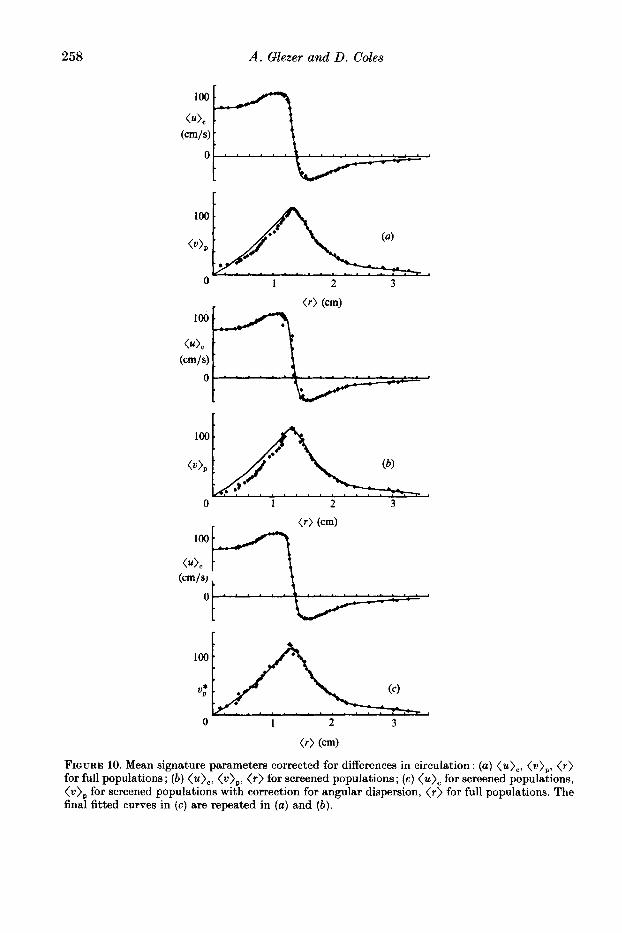
Figure lO(a) shows the dependence of the mean parameters (u), and (v), on the mean radius ( r ) for the full populations. (It was the requirement that the scatter in ( r ) in this figure be comparable with the scatter in the other variables which led, after some experimentation, to the decision to form original populations of 120 samples in figure 9(b) rather than some smaller number.) The same calculation was carried out for the screened populations, with the result shown in figure lO(b). The

t Near each end of the probe traverse, some data were missing from each histogram that would have been present if the traverse had been extended. The fitted Gaussian distributions took this fact into account, together with the fact of larger probe spacing for large r and the presence of a double measurement point on the axis of symmetry.


0 1 2 3

( r> (cm)

FIQURE 10. Mean signature parameters corrected for differences in circulation: (a) (u),, <v),, (r) for full populations; ( b ) (u),, (v),, ( r ) for screened populations; (G) (u), for screened populations, (v), for screened populations with correction for angular dispersion, ( r ) for full populations. The final fitted curves in ( c ) are repeated in (a) and ( b ) .


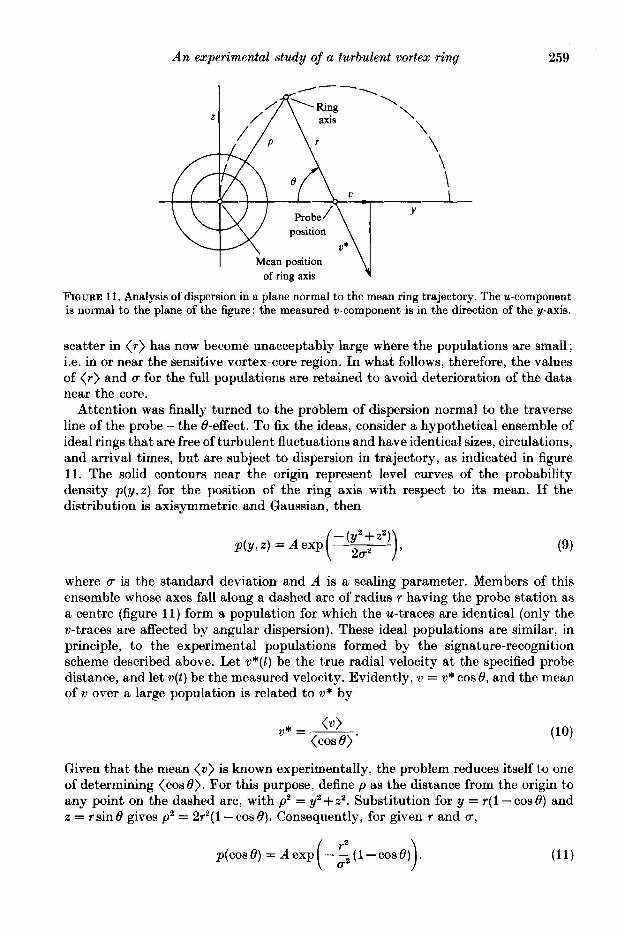
FIGURE 11. Analysis of dispersion in a plane normal to the mean ring trajectory. The u-component is normal to the plane of the figure; the measured v-component is in the direction of the y-axis.

scatter in ( r ) has now become unacceptably large where the populations are small; i.e. in or near the sensitive vortex-core region. In what follows, therefore, the values of ( r ) and u for the full populations are retained to avoid deterioration of the data near the core.

Attention was finally turned to the problem of dispersion normal to the traverse line of the probe - the 8-effect. To fix the ideas, consider a hypothetical ensemble of ideal rings that are free of turbulent fluctuations and have identical sizes, circulations, and arrival times, but are subject to dispersion in trajectory, as indicated in figure 11. The solid contours near the origin represent level curves of the probability density p(y,z) for the position of the ring axis with respect to its mean. If the distribution is axisymmetric and Gaussian, then

where u is the standard deviation and A is a scaling parameter. Members of this ensemble whose axes fall along a dashed arc of radius r having the probe station as a centre (figure 11) form a population for which the u-traces are identical (only the v-traces are affected by angular dispersion). These ideal populations are similar, in principle, to the experimental populations formed by the signature-recognition scheme described above. Let v*(t) be the true radial velocity at the specified probe distance, and let v(t) be the measured velocity. Evidently, v = v* cos 8, and the mean of v over a large population is related to w* by

Given that the mean (w) is known experimentally, the problem reduces itself to one of determining (cose). For this purpose, define p as the distance from the origin to any point on the dashed arc, with p2 = y2 + z2. Substitution for y = r ( 1 - cos 8) and z = r sin 8 gives p2 = 2r2( 1 - COB e), Consequently, for given r and u,

p(cos8) = Aexp

260 A . Clezer and D. Coles

In the present context, only positive values of cose need be considered (because all v-traces of interest lie in the upper half-plane in figure 9). The normalization condition

(12) s,'p(cos e) d cos e = i

yields

and the mean value of cose then follows as

Equation (14) has the proper limiting behaviour, namely, (cose)+ 1 as r/u+co. Another important limit, (cost?)+$ as r /a+0, reflects the fact that all values of cose between 0 and 1 tend to become equally likely when r / u is small.

It remains to associate the statistics of each real experimental population with the statistics of an associated ideal population according to the model just derived. Because the u-traces in the model population are'assumed to be identical, the data in each experimental population were first adjusted for variations in circulation by defining for each u-trace a correction factor a. This correction was designed to make the integral measure I" for each realization agree with the mean (I") for the population in question ;

(I") = r ( u ) d t = a l : u d t = a y . (15) t i

It is obvious, although not central to the argument, that (l/a) = 1. Both velocity components for each realization were multiplied by the appropriate a.

After the circulation correction just described, the remaining variation in the v- traces from one realization to another within a given population should presumably be blamed on angular dispersion and on turbulence. In an attempt to suppress the effects of turbulence, we chose to define a second correction factor p, again using an integral measure in the manner of (15) ;

The absolute value sign on the left indicates that the mean trace (v) is rectified in order to prevent the accidental vanishing of the integral (see figure 8 for some typical v-traces). The overbar on the right indicates that each individual v-trace is reflected in the t-axis (not rectified) in any time interval where (v) is negative, thus ensuring that p will be close to unity if v and (v) differ only through the presence of high- frequency fluctuations in v. The v-component for each realization was multiplied by the appropriate p.

To recapitulate, cos 8 is a dispersion factor that relates each individual v-trace in the ideal problem to the ideal trace v*. Within the limitations of the integral definition (16), 1//3 is a dispersion factor that serves the same purpose for the experimental data. The common element is the ratio r / a . As shown in figure 12 for a typical population near the axis, experimental values for r = ( r ) and u are sufficient to determine the parameter A from (13) and thus p(cos8) from (11) . The mean (cose) follows from (14). Figure 12 also shows the related histogram for 1/p after the ordinate is adjusted so that the two distributions have unit area. In order


- 0.5 0 0.5 1 .o I .5 1 (COSO) $5=cos0 or -- P (118)

F I ~ U R E 12. Probability density for dispersion parameter for ensemble 3, with ( r ) / r ~ = 0.694, f((r)/u) = 0.540.

for the real distribution to be interpreted as a noisy version of the ideal one, it is also necessary that the mean values should coincide. The proper independent variable for the experimental data is therefore not 1/p, but (1/p) (cos O ) / ( 1/p).

For the ideal distribution, (10) implies

For the real distribution, recognition of r/cr as a common element then determines the required correction :

* - (v), , v - f(./cr)

with f ( r / a ) defined by (14). Figure 10 (c ) shows the result obtained by applying (18) to the characteristic mean

parameters (w), plotted in figure lO(b).t For this purpose, as already noted, the quantities ( r ) and cr were calculated for the full populations. There is substantial improvement in the data in going from figure 10 ( b ) to 10 ( c ) , especially near the ring axis, where the ordinate values are roughly doubled. In particular, the expected nearly linear variation of w; with ( r ) near the axis finally emerges from the data. This linear variation is important because the ratio (w ) / ( r ) appears in a non-trivial way in the continuity equation and the equation for turbulence production (see (26) and (31) below).

6. Structure in similarity variables The objective of the procedures laboriously developed in the preceding section was

to invent measures for two conspicuous features of the ring signature in two dimensions. These same procedures were next applied to the whole of the data. For each of the 63 ensembles, the mean profiles obtained for (u(t)) and ( v ( t ) ) were extended to cover a time interval 1000 ms long, starting 400 ms after the trigger

t The data were inadvertently processed with an additional multiplying factor (1/p) on the right side of (18). The mean value (1/8) is not necessarily unity because of the convoluted definition (16). However, the experimental values for (I//?) lie in the range 0.98 to 1.00 for all of the 63 populatiom except for a few near the vortex core. The inadvertence affects only figure 10 (c), and the effect is small. We also failed to notice that it would have been useful a t this point to produce a perfected version of figure 9 in which the variables are taken as au, and a/3v, (with suitable adjustments to a and 8 for realizations appearing in more than one population). Dispersion in such a figure would presumably represent primarily the effect of turbulent fluctuations.

262 A . Glezer and D . Coles

FIGURE 13. Probe trajectory in (&T)-coordinates.

pulse that opened the valve, i.e. starting well before the arrival of the vortex ring at the LDV test volume. For this purpose, each data trace in an ensemble was filtered to remove grating noise, interpolated to fill dropout gaps, and smoothed by five- point averaging, as described in 94. Both velocity components were corrected for variations in circulation, i.e. multiplied by the factor a defined by (15). In addition, the v-velocity traces were corrected for angular dispersion, i.e. multiplied by the factor p defined by (16). Before the mean was calculated, the individual traces were shifted in time by the same amounts found earlier to be appropriate for shorter versions of the data. Finally, the 63 mean profiles, and the profiles in each associated population, were further shifted in time (typically by about 5 to 10 ms) to align the cursor times ( t , ) with the value measured on the axis of symmetry. The effect is to require the extremum in the u-signal to lie always in a plane through the centre of the core. The data were partially processed without this shift, but the results were unsatisfactory, particularly the check of continuity corresponding to figure 17 below.

The next and definitive step in data processing was to transform the mean velocity data to similarity variables U and V in ( E , 7)-space, as defined by (3) and (4) above. The nature of the flow, and the expectation that standard contour-plotting routines would be called, mandated use of a square grid. The associated interpolation and curve-fitting operations were designed to yield not only U and V but also aU/aq,

To simplify the notation in what follows, the apparent origin will be suppressed; i.e. t - t o will be written as t , and x-x,, will be written as x. In the same spirit, (u), (v), ( r ) , ( U ) , and ( V ) will be written as u, v, r , U , and V , respectively.

The mean velocity profiles for each ensemble describe the flow that is observed as t varies for fixed x and r. The data therefore lie along a ray through the origin in (&?)-coordinates, as indicated in figure 13, with time as the parameter along the ray. The time corresponding to the intersection of the ray with a particular grid line E = constant can be calculated from ( 3 a ) ;

au1a.g aviav, and aviag.

t = (f)($. Given t , the axial velocity u can be found by interpolation in the data, and the velocity U can be calculated from ( 4 a ) . The value of 7 at the intersection follows from the proportionality 716 = r/x .

When all of the grid lines E = constant have been treated in this way, there exists along each grid line a population of 63 values for U(7) a t irregularly spaced values of 7 (cf. figure lOc, where the variables are (u), and ( r ) ) . Let these be fitted locally by a cubic polynomial, with the fit centred on each of the various grid lines 7 = constant in turn. The result is a smooth set of values for U(7) a t the grid intersections, with a set of values for the derivative aU/aq as a byproduct.

The same procedure can be carried out for the radial velocity component to obtain V and aV/al;l.


In principle, the methods just described might also be used, after exchanging the roles of E and 7, to obtain aU/aE and aV/a t , together with redundant values for U and V . For a square grid, however, intersections of a ray with the grid lines 7 = constant are much too widely spaced to support the fitting operation. The key to proper processing then becomes the near equivalence of the time derivative and the 6- derivative along the probe trajectory in the sketch. Write (4a) as

from which

But, from (3a) and ( 3 b ) ,

Hence

and finally

au i Eau ? a 3 at 4 t at; t a7

at a t a7

+-- .

u = -(-) 1 a 3 - ( 3 u + p + q , (t- i)

Because aU/at;, aU/aq, and U / v are nominally of the same order, while 715 is not greater than about 0.02, the right-hand side of the last equation is dominated by the first term. This term corresponds to Taylor’s hypothesis, taken in this instance to mean passage of a fixed pattern past the probe at a celerity c, = (dx/dt) a t constant f;. Inasmuch as u(t) is known at equally spaced points in time, the time derivative is easily calculated. This derivative can be interpolated in t and fitted on 6 = constant to obtain values for au/at at the grid intersections, whereupon all of the quantities on the right-hand side of (25) are known, and aU/aE follows.

The same development holds, mutatis mutandis, for V. The six quantities U, V , aU/aq, aV/a7, aU/aE, aV/aE were eventually calculated on

a grid defined by 7 = 0(0.005)0.475 and E = 24.155(0.005)25.850. Contour plots for the two components of mean velocity are shown in figures 14 and 15. Note that the grid increment of 0.005 in 5 corresponds to a time interval of approximately 1 ms. Such high resolution is necessary in and near the vortex core in order to resolve large gradients in this region. Elsewhere in the flow, such high resolution is not necessary, but is maintained to accommodate the requirements of the plotting routine.

An important quantity involving derivatives is the azimuthal vorticity 5 = av/ax-au/ar. This quantity will be denoted in similarity variables by 2. From (3)

Contours for constant Z are shown in figure 16. The vorticity is strongly concentrated in the core, whose dimension (inferred from the contour representing half the peak value) is about 10% of the ring diameter.

The continuity equation in similarity variables is

au av v a t a7 7 -+-+- = 0.


0.4

0.2

t 0

0.2

0.4

24.2 24.4 24.6 24.8 25.0 25.2 25.4 25.6 25.8

5 FIQURE 14. Axial mean velocity (U) in similarity coordinates. Contour labels are -5 (1) 16,

including zero.

0.4 ' I ' ' ' ' ' ' '

24.2 24.4 24.6 24.8 25.0 25.2 25.4 25.6 25.8

5 FIQURE 15. Radial mean velocity (V) in similarity coordinates. Contour labels are -7 (1) 10,

including zero.

The experimentally determined sum on the left-hand side, shown in figure 17, is close enough to zero (e.g. smaller by a factor of 10 than the peak vorticity in the preceding figure) to inspire reasonable confidence in the accuracy of values obtained here for spatial derivatives.

The presence of turbulence in the body of the ring and in the wake is best indicated by a quantity called the intermittency, y , which is usually defined in terms of the presence or absence of small-scale fluctuations in space or time. Because the signals measured during the present experiment are statistically neither stationary nor homogeneous, a local criterion had to be developed. Given a uniformly spaced time series, consider a least-squares fit of a straight line to three successive data points, as shown in figure 18. The fitted line is parallel to a line through the first and third points. The r.m.s. deviation of the three points from the line is .\/2/61u,-2u2+u3l.

To implement this calculation for the variable u(t), each raw-data trace in an ensemble was cleared of grating noise and linearly interpolated in dropout regions,


0.4

0.2

'I 0 -

0.2

0.4

265

.

+ -

.

+ t

t o .

.

FIQURE 16. Vorticity (2) = a(v>/a[-a(U)/aq. Contour labels are 100 (100) 1200.

I

t

FIGURE 18. Least-square fit of straight line to three successive data points; d 2 s is the local r.m.8. deviation of the three points.

but not smoothed. The local r.m.5. deviation in u was computed according to the formula just given. If this deviation 8 was greater than a prescribed threshold (0.5 cm/s was chosen as a suitable value, being well above the LDV noise of about 0.05 cm/s and well below the minimum peak-to-peak excursion in w of about 9 cm/s), the flow was called turbulent, and the intermittency was set to unity for the centre


24.2 24.4 24.6 24.8 25.0 25.2 25.4 25.6 25.8

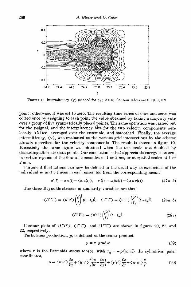
f FIGURE 19. Intermittency (7) (shaded for (7) 2 0.8). Contour labels are 0.1 (0.1) 0.9.

point; otherwise, i t was set to zero. The resulting time series of ones and zeros was edited once by assigning to each point the value obtained by taking a majority vote over a group of five symmetrically placed points. The same operation was carried out for the w-signal, and the intermittency bits for the two velocity components were locally ANDed, averaged over the ensemble, and smoothed. Finally, the average intermittency, ( y ) , was evaluated a t the various grid intersections by the scheme already described for the velocity components. The result is shown in figure 19. Essentially the same figure was obtained when the test scale was doubled by discarding alternate data points. Our conclusion is that appreciable energy is present in certain regions of the flow at timescales of 1 or 2 ms, or at spatial scales of 1 or 2 mm.

Turbulent fluctuations can now be defined in the usual way as excursions of the individual u- and w-traces in each ensemble from the corresponding mean ;

u'(t) = au(t)-(au(t)) , d ( t ) = apw(t)-(apw(t)). (27% 6)

The three Reynolds stresses in similarity variables are then

(U'u') = (u'u') G)" - ( t - t$ , (V'V') = (w'w') ($ - ( t - t0 )$ ,

1

(UV') = (u'w') - @-to): . (g Contour plots of (U'U'), (V'V'), and (U'V') are shown in figures 20, 21, and

Turbulence production, p , is defined as the scalar product 22, respectively.

p = .e-gradu (29)

where T is the Reynolds stress tensor, with rij = -p(uiu;). In cylindrical polar coordinates,

r I I au p = (uu>G+(u 'v~)


0.4

0.2

'I 0 -

0.2

0.4

267

.

.

+

.

.

_ . . . . . . . . . . I . . . . .

0.4

0.2

'I 0

0.2

0.4

24.2 24.4 24.6 24.8 25.0 25.2 25.4 25.6 25.8

5 FIGURE 21. Radial normal Reynolds stress (VV'). Contour labels are 0.5 (0.5)

0.4 t 0.2.

'I 0.

0.2 .

0.4 .

+ +

4.5.

24.2 24.4 24.6 24.8 25.0 25.2 25.4 25.6 25.8

E FIGURE 22. Reynolds shearing stress (U'V'). Contour labels are -0.7 (0.2) 0.3.


E FIGURE 23. Part of turbulence production in (31); (U'U') a(U)/ag. Contour labels are - 100, 100.

and in similarity variables

av v a7 7

+(V'V')-+(WW)-. (31)

Equation (31) differs from the corresponding equation for plane flow only in the last term, which represents stretching or shrinking of circular vortex lines in the fluid as a consequence of mean radial motions. This term was not evaluated experi- mental1y.t Contour plots of the remaining terms in (31) are shown separately in figures 23,24, 25, and 26, and the contour plot of the sum (i.e. the quantity P from (31) without the last term) is shown in figure 27. In this truncated rendition, the turbulence production is dominated by the term (VV')aV/aq. However, the missing term ( W W ) V / q is probably not negligible. The factor V / q is positive in the front half of the ring structure and negative in the rear half, as demonstrated in figure 28, and the contribution to P must have the same property. In the absence of any data, we propose to take as a plausible upper bound for (W'W) the sum of the other two Reynolds normal stresses (U'U')+(VV) (cf. figures 20 and 21). The picture of turbulence production in figure 27 is then replaced by the picture in figure 29. Roughly speaking, two contours are added (subtracted) in regions where P is large and positive (negative). In either figure, there is a conspicuous concentration of turbulence production in a small region close to and ahead of the thin vortex core. An attempt to interpret this finding physically will be postponed until some results of flow visualization have been presented in $8.

t The main data of this experiment were two extensive traverses along and normal to the optical axis at z = 42.5 cm. These traverses provided measurements of (u, w ) and (u, v), respectively. It was simply bad management that another traverse normal to the optical axis at x = 35 cm was chosen (primarily because of lower dispersion) as a vehicle for development of the signature-recognition scheme described in $5. At the end of this difficult development, our resources of energy and fiscal support were close to exhaustion. Not only would the entire analysis of this paper have had to be repeated with the main data, but new problems would have been encountered with effects of angular dispersion on the measured w-component of velocity. As a result, the opportunity was missed to observe the presence or absence of azimuthal velocities in the vortex core (cf. the conjecture by Maxworthy 1977). The question of the site and magnitude of the turbulence production is also left under a small cloud.


0.4

0.2

7 0

0.2

0.4

209 -, . . I . . . , . , , , . . . . .~ .

. -a

-+o .

.

0.4

0.2

71 0

0.2

0.4

.

. +

. +

.

0.4

0.2

?f 0 -

0.2

0.4

7 . . . , . . . . . . . . . . , .

.

. a>+@:*

. o"+@:, +::o

.

0.4

0.2

11 0 .

0.2

0.4

0.4 [

.

. ,. .-’

+ o+ . ._I ,.;a:> .

24.2 24.4 24.6 24.8 25.0 25.2 25.4 25.6 25.8

5 FIGURE 28. Mean radial velocity ( V ) / y . Contour labels are -40 (10) 50 (zero not shown).

0.4

0.2

11 0 .

0.2

0.4

- . . . . . . . . . . . . . . . . . .

,-. . ‘-8 --

+ ,</,**I 3 .__--’ cp .:I:--,

-.c

*-, . ._I

. * . . . . . . . . . . . . . . . .

An experimental study of a turbulent vortex ring 27 1

7. Particle paths and entrainment In contemporary work on coherent structures, the term entrainment is usually

understood to mean the net flow across a mean laminar-turbulent interface bounding a turbulent region. For the present case of a vortex ring, however, the interface in figure 19 and the photographic image in figure 2 ( 6 ) include a long wake of decaying turbulence that is not present in the laminar motion of figure 2(a) and is not properly part of the ring structure. The boundary has to be defined differently. The most appropriate variable for this purpose is the stream function S ( ~ , T ) whose derivatives in similarity coordinates are expressed by (4). The streamlines obtained by integration are extremely sensitive to the velocity of the observer. To track the most prominent feature of the ring, the vortex core, the observer should be moving at the (scalar) celerity C, = = 6.25 defined and evaluated in $4. The stream function is then determined by

as as - = r] (&itp), - = - y v , a t

V - dT - - -~ d t U-t l ,

or by the combination

which defines the surfaces S = constant directly. In practice, it is convenient, particularly when uniform increments of S are wanted, to take (32a) to be definitive, in which case integration yields the instantaneous streamline pattern relative to the moving vortex shown in figure 30. The feature of interest is the closed streamline S = 0 through the front and rear stagnation points, which lie a t (6, r ] ) = (24.850,O) and (25.209,O). In what follows, the instantaneous closed streamline will be taken to define the boundary of the turbulent vortex ring in terms of the mean velocity field.

The total rate of entrainment into the body of the vortex ring as just defined can be calculated immediately as the volume flux across the (transformed) boundary s = o ;

e = - J u, - nda (33)

where a is surface area, u, is fluid velocity relative to the moving boundary, and n is the outward unit normal. In a convenient vector notation, with x = (x, r ) , 5 = (6 , v ) , the velocity of any point on the boundary is dx/dt = [(dx/dt),, (dr/dt),]. Evaluation from (3) then yields

dx x dt -z ' --

Hence e = -((u-:) n da

or, after transformation and normalization,

With the aid of the divergence theorem, the last expression can be written

E = - k i v VdV+a divcdV, s


rl

0.4

0.2

0.2

0.4

24.2 24.4 24.6 24.8 25.0 25.2 25.4 25.6 25.8

5 FIUURE 30. Streamlines S = constant obtained by numerical integration of (32a). External

contour labels are 0 (0.05) 0.65; internal contour labels are 0 (-0.0125) -0.1125.

where V is the spheroidal ring volume. The first integral vanishes because div U = 0 according to (26). In the second integral, d ivt = a[/a[+ (l/r) ar2/lar = 3, so that the dimensionless entrainment becomes finally

E = aV. (38) The same result can also be obtained by a less elegant method. For simplicity,

notice that the experimental surface S = 0 is everywhere convex outward. Then the ring volume in similarity coordinates is given by

V = [l q 2 d t = constant, (39)

where E, and EO denote the rear and front stagnation points on the axis, respectively. After transformation of the right-hand side to physical coordinates, this becomes

Given that the rate of entrainment is e = dv/dt, (38) follows. The volume V and the entrainment E , like the celerity C, and the circulation G

determined in $4, are dimensionless constants of the motion, with the proviso that Vand E depend on the velocity of the observer, i.e. on the particular choice of celerity C,,. The coordinates of the spheroidal surface S = 0 in figure 30 are available experimentally. Numerical integration gives the volume as

V = 0.0480

and consequently gives the entrainment as

E = 0.0360.

It remains to indicate how this entrainment E is distributed over the boundary of the vortex ring. For this purpose, a slightly modified form of (36) is required;


where 6, = (cP,O) . This form anticipates the fact that the pair (32) for the stream function can be written as the single vector equation

1 U-K, = --grad8 x e,

where e, is the unit vector in the direction of increasing 8. The vector on the left is evidently normal to gradS (and to e,), and on the ring boundary is also normal to n. The first integral in (41) therefore vanishes, so that

E = (E-gp)*ndA. (43) i The last equation is readily interpreted. In figure 30, the difference vector <-&, is radius-like ; it represents the recession velocity in physical space of an arbitrary point on the boundary as seen by an observer at the centre of the ring volume. Mean entrainment is completely accounted for by this motion of the boundary. The only role of the fluid velocity is to define the boundary in question as the surface 8 = 0. It follows that the volume flux per unit area into the ring is essentially symmetric fore and aft, like the boundary itself, and has a weak maximum at the largest diameter. If the boundary were a sphere of radius R = lc-epl, (43) would become

E = $RA = iR(4f12) = 34.rcRs)= $J'

in agreement with (38). With the aid of some simple algebra, (38) can also be argued from (43) for the general case.

Finally, it is possible to estimate the magnitude of the entrainment velocity u, in (33) by noting the parallel construction of (33) and (43). The general scaling rule for velocity given by (4) then provides the simple proportionality

IurI als-rpl 0.05 x - x 0.008. _ - - CP CP 6.25

Thus, u, is also closely normal to the ring boundary, with a nearly uniform magnitude of less than 1 ?LO of the celerity cp.

It is very unlikely that the velocity along a particle path at the ring boundary could be evaluated experimentally with sufficient accuracy to match the discussion just given of entrainment. However, particle paths have another important use, which is to establish the topology of the coherent structure.

Particle paths in non-steady axisymmetric flow are defined by the two simultaneous

The derivatives can be expressed in similarity variables by differentiating the definitions (3);

(45a) dt

Substitution for u and v from (4) then yields the simple relationships


5 FIQURE 31. Location of critical points of (35) as intersections of the curves U = it, V = h.

where T = lnt. Except for the factor 4, which comes from the exponent carried by t in the definitions (3) for 6 and 7, these are the same equations obtained by Cantwell et al. (1978) in their study of the turbulent spot. Note that (46) are autonomous ; i.e. the right-hand sides do not depend explicitly on the time, so that they are equivalent to a single equation of the form dy/dE = F(&T,I). Consequently, while the position of a particle along its mean trajectory in ([,q)-space varies with time, the trajectory itself is independent of time.

Critical points in the flow pattern are defined by the condition dV/dt = 010, and therefore lie a t the intersections of the two curves U = 46, V = h. These two curves are plotted in figure 31. As expected, two saddle points are found at ( 6 , ~ ) = (24.849, 0) and (25.208,0), and a ring focus is found at ( 5 , ~ ) = (25.041,0.184). The two saddle points coincide, for all practical purposes, with the corresponding stagnation points in the pattern of instantaneous mean streamlines in figure 30. In physical space, the ring focus moves on a cone with an included angle of 0.0147 radians or 0.84'. The four singular points are marked by small crosses in the various contour plots to facilitate superposition and comparison of different variables in figure 14-17 and 19-30.

In previous work on the topology of coherent structures, instantaneous mean streamlines or mean particle paths have usually been determined by the method of isoclines, in which experimental values for U and I.' on a closely spaced grid generate a vector array through which integral curves are faired by eye, with due regard for the nature and location of known or suspected critical points. More recently, analytical methods have also been used. One example is the work by Perry & Tan (1984), although no details about technique are given.

In the case of mean particle paths, there is no quantity that is constant on a particular path (cf. the quantity X for a streamline). It is therefore necessary to integrate (46) simultaneously. The integration was carried out using a Runge- Kutta-Gill integrator, as described by Ralston & Wilf (1960). The reversibility of the integration along any trajectory was tested and verified. The computation normally continued until the edge of the grid was detected or until a specified number of steps was exceeded.

The initial result of the integration is displayed in figure 32. For clarity, only particle paths passing through the front and rear saddle points are shown. The curves


0.4

0.2

1 0

0.2

24.2 24.4 24.6 24.8 25.0 25.2 25.4 25.6 25.8

f FIQURE 32. Integrated particle paths (equations (46)). Only particle paths passing through the

front and rear saddle points are shown.

in figure 32 are simply not credible. The relative flow being from right to left, the computed paths imply a net de-entrainment of fluid from the rear of the ring structure into the wake. This result directly confronts the estimate of net entrainment obtained earlier in (38).

There are several possible explanations. The data may be wrong, or at least inadequate for the purpose intended. Particle paths computed from the mean velocity field may not represent correctly the mean of an ensemble of particle paths. The methods used to analyse the data may be flawed, beginning with the suppression of viscosity in the similarity argument of $4. I n what follows, the emphasis will be mainly on the last possibility.

There is no question that the critical point corresponding to the vortex-ring core is a stable focus. An expansion in vector form of the flow field near this point in similarity coordinates begins

where the derivatives are evaluated a t the critical point (&, T,,). Two important discriminants are the negative trace and the determinant of the matrix ;

au av 1 a6 ar/+2’ P = ----

If the three conditions p > 0, q > 0, and q+p2 > 0 are satisfied, the critical point is a stable focus (Perry & Fairlie 1974). The first condition follows on use of the continuity equation (26) and the definition of a critical point;

v 1 3 p = -+- = - r/ 2 4 ‘


The second condition can then be written

If i t is assumed that the flow near the critical point is essentially solid-body rotation with angular velocity +Z, where Z is the vorticity defined by (25), this becomes

q = q 2 + 1 4 8'

Thus, q > 0. Finally, according to figure 16, Z a t the focus is 0(103), and therefore q-b2 > O as well.

Circumstantial evidence for laminar flow in the vortex core includes the low values of turbulence intensity and intermittency in figures 19-21 and the photographic evidence of figure 34. Our conjecture is therefore that the similarity argument, because i t neglects viscosity, should be modified for the vortex core. For example, the size of the core might be expected to grow more like ti than like d (although it should be noted that diffusive growth of the core is not consistent with the evidence in figure 34, and in other flow visualizations, showing that the core has a sharp boundary). In the parlance of the similarity argument, the observer may be receding too slowly in this part of the flow field, although i t does not follow that the similarity argument fails in general.

To lay a foundation for a correction procedure, not that the particle-path equations (46) are invariant when rewritten for a coordinate system centred on the critical point. With E' = [-gc, 9' = 7-vc, U' = U-&, and V' = V-$rlc, these eauations become

A further transformation from rectangular coordinates (K, f), with velocity components (U', V'), to cylindrical polar coordinates (R', el), with velocity components (W', T), yields

Equations (50) show explicitly that the rate of displacement of a particle is the vector sum of the mean fluid velocity and the apparent velocity perceived by a receding observer. The use of polar coordinates confirms that only the radial equation is affected by the velocity of recession. Moreover, for a given velocity field (W', T'), the derivative dR'/dr becomes more negative, and the critical point evolves in the direction of a more stable focus, as the coefficient of the recession term becomes larger. The desired correction is implemented by modification of the recession velocity in (50a) ;

- W'-kR'-&'exp(-Rf2/2c2). (51) dR' dr --

The proper value of 8 will presumably be the one that restores order to the entrainment process. The Gaussian amplitude factor is included to ensure that the correction will be limited to the core region. The parameter c measures the size of the core in units of R'.


0.4 I 24.2 24.4 24.6 24.8 25.0 25.2 25.4 25.6 25.8

E FIUURE 33. Integrated partide paths (equations (52)). Only particle paths passing through the

front and rear saddle points are shown.

When the two transformations are undone, the corrected particle-path equations

(52 4 (E-Ec)2++(11-%)2 2a2

(46) become

dr

Note that the correction does not alter the location of the critical point, defined by dq/d[ = 0/0 at 5 = tc, 7 = vC. The core size can be estimated from figure 16 to be about 0.06 in units of 6 or 7. With this value for u, (52) were integrated, using increasing values of E , until the particle path running from the front saddle point to the focus was entirely inside the surface S = 0 (figure 33). If this particular path crossed the surface S = 0, there would be no net entrainment between the saddle point and the crossing point. The smallest satisfactory value for E was E = 20, implying that the core grows like a large power of t , a power close to E . This conclusion is not prepossessing. The best that can be said is that, even for E = 20, the magnitude of the correction term in (52) did not exceed 10% of the absolute value of the right-hand side of (46).

8. Flow visualization Resolution of the entrainment question also requires that some explanation be

found for the fact that a dyed turbulent vortex ring continuously deposits dyed fluid into its wake, aa shown, for example, in figure 2 ( b ) . Some additional flow visualization was therefore undertaken using laser-induced fluorescence and high-speed photography. The cylindrical cavity of the vortex-ring generator was filled with a solution of water-soluble fluorescent dye, and a sheet of laser light was used for illumination. Some of the results obtained are presented in figure 34. In the side view, the ring structure and wake show the apparent de-entrainment that is at issue. Then the light sheet was turned normal to the path of the ring, yielding the sequence of images shown as satellites in the figure (these are alternate frames from a movie taken at 4000 frames per 9). There is a strong suggestion of organized axial vorticity


at certain azimuthal positions. The region outside the core is either visible or not visible throughout the whole sequence, including the sections in the wake. A reasonable inference is that vortex tubes alternating in sense are wrapped around the main core in certain azimuthal planes. The presence of such vortices is consistent with the distribution of fluctuation intensity in figures 20 and 21. At some azimuthal positions, the induced flow corresponds to entrainment ; a t others, to de-entrainment. It is the latter regions that move dyed fluid into the wake, but it is the former regions that prevail in the balance. Thus, there can be a small net entrainment into the ring body. The mechanism that produces this secondary vorticity is not certain, although it may be an instability of Taylor-Gortler type. In any event, the secondary flow seems to present itself as a candidate for the next stage in a hierarchy of scales within the large coherent structure.

We note that the transition from a laminar to a turbulent vortex ring follows an azimuthal instability of the vortex core. This instability involves the appearance and amplification of azimuthal waves around the circumference of the core (Krutzsch 1939; Widnall, Bliss & Tsai 1974; Didden 1977) as the vortex moves away from the generator. The waves may subsequently break down to turbulence if their amplitude is large enough. The final stages of transition to turbulence are marked by the formation of vortex tubes similar in appearance to those observed in the present experiment (Didden 1977 ; Schneider 1980). The present flow visualization study, however, is of a fully developed turbulent ring well past the stage of transition to turbulence, whose core exhibits no azimuthal instability (figure 33). The conjecture that the formation of the vortex tubes in the present experiment is a result of a Taylor-Gortler-type instability reflects this observation.

9. Discussion From the outset of the present research, it was apparent that very little guidance

is available in the literature for experimenters who wish to design a vortex-ring generator to produce a particular kind of ring. In terms of the cylindrical-slug model of $3, the main parameters of the motion are the density and viscosity of the working fluid and the diameter, length, and velocity at the orifice of the cylindrical slug. I n a paper by Glezer (1988), a preliminary attempt was made to organize the experimental literature in terms of these parameters. The present measurements permit a few additional connections to be made, using the precepts of similarity, between the properties of a fully turbulent ring and the conditions a t the generator.

Figures 4 and 5 suggest that similarity is achieved by the time the ring has formed and moved through a distance comparable with the scale of the generator. The four points at the left in each figure were not used in the fitting operation, but are fitted well. Although these four profiles are not included in figure 6 or table 1, a t least two gross measures on the axis of symmetry (peak amplitude and peak arrival time) are consistent with similarity for t as small as 100 ms (the valve is open for 0 < t < 51 ms) and for z as small as 5 cm (the orifice diameter is 1.9 cm and the piston stroke is 6.5 cm). Fluorescent-dye pictures taken of the formation process (Glezer 1988) also suggest that the ring is very nearly mature within a few orifice diameters from the generator.

Given that the ring is nearly mature at the end of the formation process, its diameter, circulation, and celerity were computed by extrapolation backward in time to t = 51 ms. A striking property of the turbulent ring is the very slow growth rate as measured from the apparent origin. It was pointed out in $ 7 that the total


cone angle subtended by the core is 0.0147 radians. When the measured ring diameter D = 2.65 cm at x = 35 cm is extrapolated backward in time to the end of the piston stroke a t t = 51 ms, using (3b), the value obtained is 2.15 cm, as listed in table 2. Given the ratio D/(x-z , ) = 0.0147, the calculated position of the core a t the end of the piston stroke is then x = 1.3 cm (this value is obtained as the difference between two large numbers and is relatively uncertain).

Other variables that can be computed by extrapolation backward in time are the celerity cp (see the equation preceding ( 5 ) in §4), the circulation r (see (7) in §4), and the ring volume v (see (40) in $7) , defined as the volume of fluid inside the stream surface S = 0. The extrapolated values are listed in table 2, together with nominal values obtained from the cylindrical-slug model. For the turbulent vortex ring studied here, the initial celerity is about 60% of the piston velocity, the initial volume of the ring is about half of the piston displacement volume, and the initial momentum cpv is about 30% of the nominal impulse I / p calculated for the cylindrical-slug model.

The discrepancy in circulation deserves a comment. The value r = 536 cmz/s at t = 51 ms is considerably larger than the nominal value ro = 417 cmz/s associated with the cylindrical-slug model. However, this nominal circulation should probably be interpreted as a lower bound. Didden (1977, 1979) has listed two factors that can increase the circulation above the nominal value and one factor that can decrease it. The circulation is increased primarily by the fact that the velocity near the sharp corner at the generator exit must be appreciably larger than V, for small times, and also by the fact that the core flow must accelerate at large times (for constant piston velocity) because the internal boundary layer becomes thicker. A factor that can decrease the circulation is ingestion into the nascent vortex ring of vorticity of opposite sign generated by the pressure field on the external wall. Didden’s second paper is an expert experimental study of these three factors for the case of a laminar ring.

At least two experiments reported in the literature supply enough data for D(x) so that an apparent origin, and thus a cone angle, can be determined. Table 3 lists, in order of increasing circulation, values for D / ( x - zo) inferred from data obtained by these authors. Johnson (1970) used smoke for flow visualization and recorded ring position photographically. In Johnson’s data (see his figure 7) , there is a curious small zigzag variation in D(x) for all five rings, slightly impairing the present application of his measurements. Johnson’s position on the question of similarity was ambivalent, and in a short journal publication (1971) he abandoned similarity in favour of empirical power laws. Sallet & Widmayer (1974) reported data for the three turbulent rings listed in table 3. For these experiments, the circulation calculated according to the cylindrical-slug model has been adjusted to take into account the triangular piston-velocity program. The apparent origin xo has been estimated from the observed celerity, which follows the similarity law. The observed ring growth is not linear, and only the two most downstream stations have been used to represent D(s) . For reasons just explained, it is likely that the circulation r , / v is underestimated in the table, the more so as the ratio Lo/Do becomes smaller.

An occasional ellipsis in the design of the present research is worth mentioning. Our reasons for our failure to measure the third (azimuthal) velocity component have already been set out in $6; one consequence is incomplete documentation of the turbulence production. Larger statistical populations would certainly be useful in reducing the scatter of the data and in yielding a better representation of various quantities involving higher statistical moments. For example, several irregularities


Measured at Extrapolated to Cylindrical-slug model x = 35.0 cm t = 693 ms t = 5 1 m s Value Formula

x = 1.3 cm

Ring diameter (cm) 2.65 2.15 1.9 DO

Celerity (cm/s\ 39.7 74.4 127.8 4

Circulation (cmz/s) , 353.0 536.0 417.0 ro=fqx r = 7.71(1/p)~ ( t - t p

D = 0.368(l/p)S ( t - to)f

cp = 6.25(1/p)z ( t - to)-!

Volume (cm3) 17.9 9.57 18.6 V,=$@Z& v = 0.048(I/p)i ( t - to):

TABLE 2. Estimated ring parameters near the orifice

Source Johnson (1970) (case 5) Sallet & Widmayer (1974) (26 ms) Sallet & Widmayer (1974) (20 ms) Sallet & Widmayer (1974) (18 ms) Johnson (1970) (case 4) Present work Johnson (1970) (case 3) Johnson (1970) (case 2) Johnson (1970) (rase 1 )

LOlDO 0.78 1.33 1.33 1.33 1.50 3.42 1.56 3.13 3.13

TO/ V 13900 17 800 23 200 25 700 40 100 41 700 44 300 93 100

102 000

Dl(x-xo) 0.0149 0.0168 0.0147 0.0135 0.0145 0.0147 0.01 12 0.0103 0.0091

TABLE 3. Growth rate of turbulent vortex rings

in the contour plots, beginning with figures 14 and 15, are directly traceable to thin spots in the main sequence in figure 9. However, to obtain statistical populations larger by an order of magnitude would have increased the working time to unreasonable values, perhaps 20 to 30 working hours at each probe station. A more effective strategy might be to use air as a working fluid and a flying hot wire w main instrumentation. It would also have been better (in hindsight) to carry out a full two- sided traverse, to enforce equal spacing for the probe stations, and to go to larger radii. The anomalous curvature a t large radii in the streamlines of figure 30 is almost certainly caused by non-uniform spacing of the probe stations in this region.

In another incarnation, we would make one major revision in data processing ; this is t o avoid treating the u- and v-signals differently and separately. This practice was thought initially to be necessary because one effect of angular dispersion is to bias the w-traces toward low values, and a policy of discarding the tails of each distribution would distort this bias. Classification of ring signature into populations was done by shifting the data slightly in time and adjusting the amplitude of the u-traces so as to normalize the peak arrival time and the integral magnitude. However, resulting jitter in the v-traces was not accounted for. The derivative (aU/aq) is therefore sharply resolved in the calculation of vorticity from (25), but the derivative (aV/a€J is smeared, and the vorticity contours are distorted in figure 16 (smoke or dye visualization by various experimenters, as in figure 34, uniformly shows an essentially circular cross-section for a thin core). Moreover, the intermittency in figure 19 and the normal Reynolds stress (V'V') in figure 21 are forced toward values that are too large in and near the vortex core.


The problem of dispersion was always in the foreground in the present research, and heroic measures were necessary to deal with it. In most previous work on the turbulent vortex ring, serious problems with dispersion either are reported or can be inferred from the nature of the published data. In several cases in the literature, furthermore, the results are made less useful by effects of probe interference and/or directional ambiguity in the measurements of velocity, whether the main instrumentation was the hot-wire anemometer or the laser-Doppler velocimeter.

Solution of these problems in the research reported here has provided solid evidence in support of the concept of similarity in any description of the turbulent vortex ring. A property of the ring that was not expected is the dominant role in the turbulence production of the turbulent normal stresses, especially the measured term (V'V') a( V)/a.l;l and the estimated term (W'W') ( V ) / q . In figure 29, it is significant that the production is largest in the forward half of the ring volume, where vortex stretching is an important part of the dynamics. Another useful inference is that secondary vorticity in azimuthal planes is important for entrainment. Finally, it is likely that several delicate issues raised in 97 in the discussion of topology and entrainment will recur in future work on coherent structures in other flows, particular structures characterized by slow growth and by a diminished role for the process of coalescence.

The assistance of Dr Thomas Roesgen in making the various contour plots is deeply appreciated. The research described in this paper was supported in part by the National Science Foundation under Grants ENG 75-03694 and ENG 77-23541.

R E F E R E N C E S AKHMETOV, D. G. & KISAROV, 0. P. 1966 Hydrodynamic structure of a vortex ring. J . Appl. Mech.

Tech. Phys. 7 , 87-90. CANTWELL, B., COLES, D. 6 DIMOTAKIS, P. 1978 Structure and entrainment in the plane of

symmetry of a turbulent spot. J . Fluid Mech. 87, 641-672. DIDDEN, N. 1977 Untersuchung laminarer, instabiler Ringwirbel mittels Laser-Doppler-

Anemometrie. Dissertation, University of Gottingen ; also Mitt . MPI und AVA, Giittingen, Nr. 64.

DIDDEN, N. 1979 On the formation of vortex rings: rolling-up and production of circulation. 2. Angew. Math. Phys. 30, 101-116.

GLEZER, A. 1981 An experimental study of a turbulent vortex ring. Ph.D. thesis, California Institute of Technology.

GLEZER, A. 1988 On the formation of vortex rings. Phys. Fluids 31, 3532-3542. GLEZER, A. 6 COLES, I>. 1982 A two-grating method for combined beam splitting and frequency

shifting in a two-component laser-Doppler velocimeter. Phys. Fluids 25, 2142-2146. GRIGG, H. R. & STEWART, R. W. 1963 Turbulent diffusion in a stratified fluid. J . Fluid Mech. 15,

JOHNSON, G . M. 1970 Researches on the propagation and decay of vortex rings. Rep. ARL 70- 0093. Aerosp. Res. Labs., Wright-Patterson AFB.

JOHNSON, G. M. 1971 An empirical model of turbulent vortex rings. AZAA J . 9, 763-764. KOVASZNAY, L. S. G., FUJITA, H. 6 LEE, R. L. 1973 Unsteady turbulent puffs. Adw. Geophys.

KRUTZCH, C. H . 1939 Uber eine experimentele beobachtete Erscheinung an Wirbelringen bei ihrer

MAXWORTHY, T. 1974 Turbulent vortex rings. J . Fluid Mech. 64, 227-239. MAXWORTHY, T. 1977 Some experimental studies of vortex rings. J . Fluid Mech. 81, 465-495. NORTHRUP, E. F. 1912 A photographic study of vortex rings in liquids. Nature 88, 463468.

174-1 86.

18B, 253-263.

translatorischen Bewegung in Wirklichen Fliissigkeiten. Ann. Phye. 35, 497-523.


OSHIMA, K., KOVASZNAY, L. S. G. & OSHIMA, Y. 1977 Sound emission from burning puff. In Proceedings, Symposium on Structure and Mechanisms of Turbulence, Vol. I1 (ed. H. Fielder). Lecture Notes in Physics, vol. 76, pp. 214-230. Springer.

PERRY, A. E. & FAIRLIE, B. D. 1974 Critical points in flow patterns. Adv. Geophys. 18B, 29S315. PERRY, A. E. & TAN, D. K. M. 1984 Simple three-dimensional vortex motions in coflowing jets

RALSTON, A. & WILF, H. S. 1960 Mathematical Methods for Digital Computers. John Wiley & Sons. RICHARDS, J. M. 1965 Puff motions in unstratified surroundings. J. Fluid Mech. 21, 97-106. SAFFMAN, P. G. 1970 The velocity of viscous vortex rings. Stud. Appl. M a t h 49, 371-380. SALLET, D. W. & WIDMAYER, R. S. 1974 An experimental investigation of laminar and turbulent

SCHNEIDER, P. 1980 Sekundanvirbelbildung bei Ringwirbeln und in Freistrahlen. 2. Flugwiss.

SULLIVAN, J. P., WIDNALL, S. E. & EZEKIEL, S. 1973 Study of a vortex ring using laser Doppler

TURNER, J. S. 1957 Buoyant vortex rings. Proc. R. SOC. Lond. A 239, 61-75. TURNER, J. S. 1964 The flow into an expanding spherical vortex. J. Fluid Mech. 18, 195-208. WZDNALL, S. E., BLISS, D. B. & TSAI, C.-Y. 1974 The instability of short waves on a vortex ring.

WOODWARD, B. 1959 The motion in and around isolated thermals. &. J. R. Met. SOC. 85, 14P151.

and wakes. J. Fluid Mech. 141, 197-231.

vortex rings in air. 2. Flugwiss. 22, 207-215.

Weltraumforsch. 4, 307-3 18.

velocimeter. AIAA J. 11, 1384-1389.

J . Fluid Mech. 66, 35-47.

FLM 211

by ari glezerl and donald coles2 - california...

Documents