DATA-SNOOPING BIASES IN TESTS OF FINANCIAL

ASSET PRICING MODELS

by

Andrew W. Lo and A. Craig MacKinlay

Latest Revision: November 1989

Revised Working Paper No. 3020-89-EFA

DATA-SNOOPING BIASES IN TESTS OF FINANCIAL ASSET PRICING MODELS

Andrew W. Lo* and A. Craig MacKinlay**

First Draft: February 1989Latest Revision: November 1989

We investigate the extent to which tests of financial asset pricing models may be biased byusing properties of the data to construct the test statistics. Specifically, we focus on testsusing returns to portfolios of common stock where portfolios are constructed by sorting onsome empirically motivated characteristic of the securities such as market value of equity.We present both analytical calculations and Monte Carlo simulations that show the effectsof this type of data-snooping to be substantial. Even when the sorting characteristic is onlymarginally correlated with individual security statistics, 5 percent tests based on sortedportfolio returns may reject with probability one under the null hypothesis. This bias isshown to worsen as the number of securities increases given a fixed number of portfolios,and as the number of portfolios decreases given a fixed number of securities. We providetwo empirical examples that illustrate the practical relevance of these biases.

*Sloan School of Management, Massachusetts Institute of Technology.**Department of Finance, Wharton School, University of Pennsylvania.

We thank David Aldous, Cliff Ball, Herbert David, Mike Gibbons, a referee, and seminar participants at the Boardof Governors of the Federal Reserve, Columbia, Dartmouth, M.I.T., Northwestern, Princeton, Stanford, the University ofChicago, the University of Michigan, the University of Wisconsin at Madison, and Wharton for useful comments and suggestions.Research support from the Batterymarch Fellowship (Lo), the Geewax-Terker Research Fund (MacKinlay), the John M. OlinFellowship at the National Bureau of Economic Research (Lo), and the National Science Foundation (SES-8821583) is gratefullyacknowledged.

1. Introduction.

The reliance of economic science upon non-experimental inference is, at once, one of

the most challenging and most nettlesome aspects of the discipline. Because of the virtual

impossibility of controlled experimentation in economics, the importance and influence

of statistical data analysis is now well-established. However, there is a growing concern

that the procedures under which formal statistical inference have been developed may not

correspond to those followed in practice.1 For example, the classical statistical approach to

selecting a method of estimation generally involves minimizing an expected loss function

irrespective of the actual data at hand. Yet in practice the properties of the realized data

almost always influence the choice of estimator.

Of course, ignoring obvious features of the data can lead to nonsensical inferences even

when the estimation procedures are optimal in some metric. But the way we incorporate

those features into our estimation and testing strategies can affect subsequent inferences

considerably. Indeed, by the very nature of empirical innovation in economics, the axioms

of classical statistical analysis are violated routinely: future research is often motivated by

the successes and failures of past investigations. Consequently, few empirical studies are

free of the kind of data-instigated pre-test biases discussed in Leamer (1978). Moreover,

we should expect the degree of such biases to be an increasing function of the number of

published studies performed on any single data set. The more scrutiny a collection of data

is subjected to, the more likely will interesting (spurious) patterns emerge. Since stock

market prices are perhaps the most studied economic quantities to date, tests of financial

asset pricing models seem especially susceptible.

In this paper we attempt to quantify the inferential biases associated with one par-

ticular method of testing financial asset pricing models, such as the Capital Asset Pricing

Model (CAPM) and the Arbitrage Pricing Theory (APT). Because there are often many

more securities than there are time series observations of stock returns, asset pricing tests

are generally performed on the returns of portfolios of securities. Besides reducing the

cross-sectional dimension of the joint distribution of returns, grouping into portfolios has

also been advanced as a method of reducing the impact of measurement error.2 However,

1 Perhaps the most complete analysis of such issues in economic applications is given by Leamer (1978). Recent papers byLakonishok and Smidt (1988), Merton (1987), and Ross (1987) address data-snooping in financial economics. Of course, data-snooping has been a concern among probabilists and statisticians for quite some time, and is at least as old as the controversybetween Bayesian and classical statisticians. A satisfactory discussion of such issues would take us too far afield, but interestedreaders should consult Berger and Wolpert (1984, Chapter 4.2) and Leamer (1978, Chapter 9) for further details.

2 Blume (1970) was perhaps the first to suggest this. See also Black, Jensen, and Scholes (1972) and Fama and MacBeth(1973).

7.7 -1- 11.89

III

the selection of securities to be included in a given portfolio is almost never at random,

but is often based on some of the stocks' empirical characteristics. The formation of size-

sorted portfolios, portfolios based on the market value of the companies' equity, is but

one example. Constructing classical statistical tests on portfolios formed this way creates

potentially significant biases in the test statistics. These are examples of "data-snooping

statistics," a term used by Aldous (1989, p. 252) to describe the situation "where you have

a family of test statistics T(a) whose null distribution is known for fixed a, but where you

use the test statistic T = T(a) for some a chosen using the data." In our application the

quantity a may be viewed as a vector of zeros and ones that indicates which securities are

to be included in or omitted from a given portfolio. If the choice of a is based on the data,

then the sampling distribution of the resulting test statistic is generally not the same as

the null distribution with a fixed a; hence, the actual size of the test may differ substan-

tially from its nominal value under the null. Under plausible assumptions our calculations

show that this kind of data-snooping can lead to rejections of the null hypothesis with

probability one when the null hypothesis is true!

Although the term "data-snooping" may have an unsavory connotation, our usage

neither implies nor infers any sort of intentional misrepresentation or dishonesty. That

prior empirical research may influence the way current investigations are conducted is often

unavoidable, and this very fact results in what we have called data-snooping. Moreover, it

is not at all apparent that this phenomenon necessarily imparts a "bias" in the sense that

it affects inferences in an undesirable way. After all, the primary reason for publishing

scientific discoveries is to add to a store of common knowledge on which future research

may build.

However, when scientific discovery is statistical in nature, we must weigh the signifi-

cance of newly discovered relations in view of past inferences. This is recognized implicitly

in many formal statistical circumstances, as in the theory of sequential hypothesis test-

ing. 3 But it is considerably more difficult to correct for the effects of specification searches

in practice since such searches often consist of sequences of empirical studies undertaken

by many individuals.4 For example, as a consequence of the many investigations relating

the behavior of stock returns to size, Chen, Roll and Ross (1986, p. 394) write: "It has

been facetiously noted that size may be the best theory we now have of expected returns.

8 The classic reference is Wald (1947); see Siegmund (1985) for more recent developments.4 Statisticians have considered a closely related problem, known as the "file drawer problem," in which the overall significance

of several published studies must be assessed while accounting for the possibility of unreported insignificant studies languishingin various investigators' file drawers. An excellent review of the file drawer problem and its remedies, which has come to beknown as "meta-analysis," is provided by Iyengar and Greenhouse (1988).

7.7 - 2- 11.89

Unfortunately, this is less of a. theory than an empirical observation." Then, as Merton

(1987, p. 107) asks in a related context: "Is it reasonable to use the standard t-statistic

as a valid measure of significance when the test is conducted on the same data used by

many earlier studies whose results influenced the choice of theory to be tested?" We re-

phrase this question in the following way: Are standard tests of significance valid when

the construction of the test statistics is influenced by empirical relations derived from the

very same data to be used in the test? Our results show that using prior information only

marginally correlated with statistics of interest can distort inferences dramatically.

In Section 2 we quantify the data-snooping biases associated with testing financial

asset pricing models with portfolios formed by sorting on some empirically motivated

characteristic. Using the theory of induced order statistics, we derive in closed-form the

asymptotic distribution of a commonly-used test statistic before and after sorting. This

not only yields a measure of the effect of data-snooping, but aiso provides the appropriate

sampling theory when snooping is unavoidable. In Section 3 we report the results of Monte

Carlo experiments designed to gauge the accuracy of the previous section's asymptotic

approximations. Section 4 provides two empirical examples that illustrate the potential

importance of data-snooping biases in existing tests of asset pricing models, and Section

5 shows how these biases can arise naturally from our tendency to focus on the unusual.

We conclude in Section 6.

-3-7.7 11.89

Ill

2. Quantifying Data-Snooping Biases With Induced Order Statistics.

Many tests of the CAPM and APT have been conducted on returns of groups of se-

curities rather than on individual security returns, where the grouping is often according

to some empirical characteristic of the securities. Perhaps the most common attribute

by which securities are grouped is market value of equity or "size." 5 The prevalence of

size-sorted portfolios in recent tests of asset-pricing models has not been precipitated by

any economic theory linking size to asset prices. It is a consequence of a series of empirical

studies demonstrating the statistical relation between size and the stochastic behavior of

stock returns. 6 Therefore, we must allow for our foreknowledge of size-related phenomena

in evaluating the actual significance of tests performed on size-sorted portfolios. More

generally, grouping securities by some characteristic that is empirically motivated may af-

fect the size of the usual significance tests,7 particularly when the empirical motivation is

derived from the very data set on which the test is based. We quantify these effects in the

following sections by appealing to asymptotic results for induced order statistics, and show

that even mild forms of data-snooping can change inferences substantially. Section 2.1 pro-

vides a brief summary of the asymptotic properties of induced order statistics. Section

2.2 presents results for tests based on individual securities, and Section 2.3 reports corre-

sponding results for portfolios. In Section 2.3 we provide a more positive interpretation of

data-snooping biases as power against deviations from the null hypothesis.

2.1. Asymptotic Properties of Induced Order Statistics.

Since the particular form of data-snooping we are investigating is most common in

empirical tests of financial asset pricing models, our exposition will lie in that context.

Suppose for each of N securities we have some consistent estimator &i of a parameter ai

which is to be used in the construction of an aggregate test statistic. For example, in the

Sharpe-Lintner CAPM &i would be the estimated intercept from the following regression:

R1t-Rft = ci + (Rmt- Rft) i + Eit (2.1)

5 The following is only a partial list of the more recent studies using size-sorted portfolios: Chan and Chen (1988), Chan,Chen, and Hsieh (1985), Chen, Roll, and Ross (1986), Connor and Korajczyk (1988), Kandel and Stambaugh (1987), Lehmannand Modest (1988), MacKinlay (1987), and Shanken (1985).

See Banz (1981), Brown, Kleidon, and Marsh (1983), and Chan, Chen, and Hsieh (1985) for example.7 Unfortunately the use of size" to mean both market value of equity and type I error is unavoidable. Readers beware.

7.7 -4- 11.89

where R/t, Rmt, and Rft are the period-t returns on security i, the market portfolio, and

a risk-free asset respectively. A test of the null hypothesis that ai = 0 would then be

a proper test of the Sharpe-Lintner version of the CAPM; thus, &/ may serve as a test

statistic itself. However, more powerful tests may be obtained by combining the &i's for

many securities. But how to combine them?

Suppose for each security i we observe some characteristic Xi, such as its out-of-sample

market value of equity or average annual earnings, and we learn that X i is correlated em-

pirically with &j. By this we mean that the relation between Xi and &i is an empirical fact

uncovered by "searching" through the data, and not motivated by any a priori theoreti-

cal considerations. This search need not be a systematic sifting of the data, but may be

interpreted as any one of Leamer's (1978) six specification searches which even the most

meticulous of classical statisticians has conducted at some point. The key feature is that

our interest in characteristic X i is derived from a look at the data, the same data to be

used in performing our test. Common intuition suggests that using information contained

in the X i 's can yield a more powerful test of economic restrictions on the &j's. But if this

characteristic is not a part of the original null hypothesis, and only catches our attention

after a look at the data (or after a look at another's look at the data), using it to form

our test statistics may lead us to reject those economic restrictions even when they obtain.

More formally, if we write &i as:

= ai + A (2.2)

then it is evident that, under the null hypothesis where ai = 0, any correlation between X i

and &i must be due to correlation between the characteristic and estimation or measure-

ment error i. Although measurement error is usually assumed to be independent of all

other relevant economic variables, the very process by which the characteristic comes to

our attention may induce spurious correlation between X i and i. We formalize this intu-

ition in Section 5, and proceed now to show that such spurious correlation has important

implications for testing the null hypothesis.

This is most evident in the extreme case where the null hypothesis a i = 0 is tested by

performing a standard t-test on the largest of the &i's. Clearly such a test is biased toward

rejection unless we account for the fact that the largest &i has been drawn from the set

&i}. Otherwise, extreme realizations of estimation error will be confused with a violation

7.7 - 5 - 11.89

III

of the null hypothesis. If instead of choosing &i based on its value relative to other a&'s

our choice is based on some characteristic Xi correlated with the estimation errors of &i,

a similar bias might arise, albeit to a lesser degree.

To formalize the preceding intuition, suppose that only a subset of n securities are

used to form the test statistic and these n are chosen by sorting the Xi's. That is, let us

re-order the bivariate vectors [Xi &i]' according to their first components, yielding the

sequence:

X1N X2N ... XN:N (2.3)all:N/ [2:N / [N:N/

where X1:N < X2:N < .."' < XN:N and the notation Xi:N follows that of the

statistics literature in denoting the i-th order statistic from the sample of N observations

{Xi}. 8 The notation [i:N] denotes the i-th induced order statistic corresponding to Xi:N,

or the i-th concomitant of the order statistic Xi:N.9 That is, if the bivariate vectors

[Xi &i]' are ordered according to the X i entries, &[i:N] is defined to be the second

component of the i-th ordered vector. The &[i:N] are not themselves ordered but correspond

to the ordering of the Xi:N's.l 0 We call this procedure induced ordering of the &i's. It

is apparent that if we construct a test statistic by choosing n securities according to the

ordering (2.3) the sampling theory cannot be the same as that of n securities selected

independently of the data. Due to the following remarkably simple result by Yang (1977),

an asymptotic sampling theory for test statistics based on induced order statistics may be

derived analytically:11

8 It is implicitly assumed throughout that both &i and Xi have continuous joint and marginal c.d.f.'s, hence strict inequalitiessuffice.

9The term concomitant of an order statistic was introduced by David (1973), who was perhaps the first to systematicallyinvestigate its properties and applications. The term induced order statistic was coined by Bhattacharya (1974) at about thesame time. Although the former term seems to be more common usage, we use the latter in the interest of brevity. SeeBhattacharya (1984) for an excellent review.

0°If the vectors are independently and identically distributed and Xi is perfectly correlated with &, then &i:N are alsoorder statistics. But as long as the correlation coefficient p is strictly between -1 and 1 then, for example, &IN:N] will generallynot be the largest &i. In fact, it may readily be shown that for any fixed k:

plim (2a21logN)- / 2XN_k:N = 1 , plim (20 logN)/2&IN._kN = PN-oo N-.oo

thus the largest Xi is almost never paired with the largest &i. See David (1981), David, O'Connell, and Yang (1977) andGalambos (1987) for further details.

1 1 See also David and Galambos (1974) and Watterson (1959). Yang (1977) provides the exact finite-sample distribution ofany finite collection of induced order statistics, but even assuming bivariate normality does not yield a tractable form for thisdistribution. For example, the exact joint c.d.f. of the i-th and j-th induced order statistics is given by:

a - a -p \(Xi:Nl r-ai - a - (Xj:N- )1Pr(&;,:N) < a;, &Lj:N < aj) = E a - (1 p2) `) P2 )

11.897.7 -6-

Theorem 2.1. Let the vectors [Xi &d]'l, i = 1,...,N be independently and identically

distributed and let 1 < i < i 2 < ... < in < N be sequences of integers such that, as

N -- oo, ik/N -, k E (, 1) (k = 1,2,..., n). Then

n

lim Pr(&[il:N] < al,... &[i: N < an) = Pr(k < aklF(Xk)= k) (2.4)k=l

where F,(-) is the marginal c.d.f. of X i .

Proof. See Yang (1977).

I

This result gives the large-sample joint distribution of a finite subset of induced order

statistics whose identities are determined solely by their relative rankings k (as ranked

according to the order statistics Xi:N). From (2.4) it is evident that {&[i:NI} are mutually

independent in large samples. If X i were the market value of equity, or "size," of the i-th

security Theorem 2.1 shows that the &i of the security with size at the 27-th percentile is

asymptotically independent of the &j corresponding to the security with size at the 45-th

percentile, for example.12 If the characteristics {Xi} and {&c} are statistically independent,

the joint distribution of the latter clearly cannot be influenced by ordering according to

the former. It is tempting to conclude that as long as the correlation between X i and &i is

economically small, induced ordering cannot greatly affect inferences. Using Yang's result

we show the fallacy of this argument in Sections 2.2 and 2.3.

2.2. Biases of Tests Based on Individual Securities.

We evaluate the bias of induced ordering under the following assumption:1 3

where 0(.) is the standard normal c.d.f. and the expectation is taken with respect to the joint distribution of the order statistics

(Xi:N, Xj:N).12 This is a limiting result and, in particular, implies that the identities of the stocks with 27-th and 45-th percentile sizes

generally will change as N increases.18 Some of our results are robust to this parametric specification. For example, if we replace normality by the assumption

that &i and Xi satisfy the linear regression equation:

i = 1 + (Xi-is.) + Zi

where Zi is independent of Xi, then our results remain unchanged. Moreover, this specification may allow us to relax therather strong i.i.d. assumption, since David (1981, chapters 2.8 and 5.6) does present some results for order statistics in thenon-identically distributed and the dependent cases separately. However, combining and applying them to the above linearregression relation is a formidable task which we leave to the more industrious.

1~ ~~ ------ _

7.7 -7- 11.89

The simplicity of i's asymptotic distribution follows from the fact that the &[ik :N's

become independent as N increases without bound. The intuition for this seemingly

counterintuitive result follows directly from the bivariate normality of [ X i &i ], which

implies:

&i = + Pa X- ]+zi Zi idi N (0, (1 _ P~(2)) (2.12)

where Xi and Zi are independent. Therefore, the induced order statistics may be repre-

sented as:

&Ii,:N] = + P [Xik:N - Itx] + Z , Zlij .i.d. N (0,u(1 - p2)) (2.13)

where the Zi are independent of the (order) statistics Xik:N. But since Xik:N is an

order statistic, and since the sequence ikiN converges to k, Xik:N converges to the k-th

quantile, F-l(k). Using (2.13) yields the limiting distribution of &[ik:N] to be Gaussian,

with mean and variance given by (2.8) and (2.9).

To evaluate the size of a 5 percent test based on the statistic we need only evaluate

the c.d.f. of the non-central x2(A) at the point C 5/(1 _- p2 ), where C" 5 is given in (2.6).

Observe that the non-centrality parameter A is an increasing function of p2 . If p2 = 0 then

the distribution of reduces to a central X2 which is identical to the distribution of in

(2.5); sorting on a characteristic that is statistically independent of the &i's cannot affect

the null distribution of theta. As &i and Xi become more highly correlated, the non-central

x 2 distribution shifts to the right. However, this does not imply that the actual size of a 5

percent test necessarily increases since the relevant critical value for , C.6 5/(1 - p2 ), also

grows with p2. 17

17 In fact, if p2 = 1 the limiting distribution of j is degenerate since the test statistic converges in probability to the followinglimit:

E= [1-'((h)]

This limit may be greater or less than C. s depending on the values of ~k, hence the size of the test in this case may be eithersero or unity.

7.7 - 10- 11.89

��I__ �

Numerical values for the size of a 5 percent test based on may be obtained by first

specifying choices for the relative ranks { k} of the n securities. We consider three sets of

{k}, yielding three distinct test statistics 81, 2, and 03:

01 k = k (2.14)n+l

f(+k for k = 1,2,...,no.82 X = m * (2.15)

02 X{k = ( + m(no+l) no

where n _ 2no and no is an arbitrary positive integer. The first method (2.14) simply sets

the k's so that they divide the unit interval into n equally-spaced increments. The second

procedure (2.15) first divides the unit interval into m + 1 equally-spaced increments, sets

the first half of the k's to divide the first such increment into equally-spaced intervals

each of width 1/(m + )(no + 1), and then sets the remaining half so as to divide the

last increment into equally-spaced intervals also of width 1/(m + 1)(no + 1) each. The

third procedure is similar to the second, except that the ek's are chosen to divide the

second smallest and second largest m + 1-increments into equally spaced intervals of width

1/(m + 1)(no + 1).

These three ways of choosing n securities allow us to see how an attempt to create (or

remove) dispersion-as measured by the characteristic Xnto - affects the null distribution of

the statistics. The first choice for the relative ranks is the most disperse, being evenly dis-

tributed on (0,1). The second yields the opposite extreme: the &alfN selected are those

with characteristics in the lowest and highest 100/(m + 1)-percentiles. As the parameter

m is increased, more extreme lowest are used to100/ + )-percen2. This is also true for 3, but

to a lesser extent since the statistic is based on &[i:N]'S in the second lowest and second

highest 100/(m + 1)-percentiles.

7.7 11.89- 11-

Table 1 reports the size of the 5 percent test using 01, 02, and 03 for various values

of n, p2 , and m. For concreteness, observe that p2 is simply the R 2 of the cross-sectional

regression of &i on Xi, so that p = .10 implies that only 1 percent of the variation in &i

is explained by X i . For this value of R 2 , the entries in the first panel of Table 1 show that

the size of a 5 percent test using 01 is indeed 5 percent for samples of 10 to 100 securities.

However, using securities with extreme characteristics does affect the size, as the entries in

the '0 2-Test' and '0 3 -Test' columns indicate. Nevertheless the largest deviation is only 8.1

percent. As expected, the size is larger for the test based on 02 than for that of 03 since

the former statistic is based on more extreme induced order statistics than the latter.

When the R 2 increases to 10 percent the bias becomes more important. Although tests

based on a set of securities with evenly-spaced characteristics still have sizes approximately

equal to their nominal 5 percent value, the size deviates more substantially when securities

with extreme characteristics are used. For example, the size of the 02 test that uses the 100

securities in the lowest and highest characteristic-decile is 42.3 percent! In comparison,

the 5 percent test based on the second lowest and highest two deciles exhibits only a 5.8

percent rejection rate. These patterns become even more pronounced for R 2 's higher than

10 percent.

The intuition for these results may be found in (2.8): the more extreme induced order

statistics have means farther away from zero, hence a statistic based on evenly-distributed

&[i:N]'s will not provide evidence against the null hypothesis a = 0. If the relative ranks

are extreme, as is the case for 02 and 03, the resulting &[i:N]'s may appear to be statistically

incompatible with the null.

2.3. Biases of Tests Based on Portfolios of Securities.

The entries in Table 1 show that as long as the n securities chosen have characteristics

evenly distributed in relative rankings, test statistics based on individual securities yield

little inferential bias. However, in practice the ordering by characteristics such as market

value of equity is used to group securities into portfolios and the portfolio returns are used

to construct test statistics. For example, let n noq where no and q are arbitrary positive

integers, and consider forming q portfolios with no securities in each portfolio where the

securities are chosen independently of the data. Under the null hypothesis H we have the

following:

7.7 - 12 - 11.89

____II___________I____1___1____�1___�___ ___�Y·�_�_I__C�

(2.17)k ~ N(o, a j=(k-)no+l no

q

p-- a E q X 2 (2.18)k=1

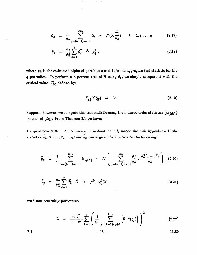
where 4 k is the estimated alpha of portfolio k and Op is the aggregate test statistic for the

q portfolios. To perform a 5 percent test of H using p, we simply compare it with the

critical value Cq5 defined by:

FXq2(C.oS) = 95 (2.19)

Suppose, however, we compute this test statistic using the induced order statistics {&[i:N]}instead of {&i}. From Theorem 2.1 we have:

Proposition 2.2. As N increases without bound, under the null hypothesis H the

statistics qk (k = 1, 2, ... , q) and Op converge in distribution to the following:

kno

j=(k- 1)no+l&lij:N] N (

k _n_, 2~(1 - p2)j=(k-l)no+l no no(2.20)no n)

(2.21)

np2 q) -op2 X -- " kp2

7.7

1 knjk

j=(k-l)no+l

- 13 -

P = 2 d (1 _ p2 ) X(A)

with non-centrality parameter:

[a'(j 2)]

['l 1 )0 (2.22)

11.89

The non-centrality parameter (2.22) is similar to that of the statistic based on individual

securities; it is increasing in p2 and reduces to the central X2 of (2.22) when p = 0. However,

it differs in one respect: because of portfolio aggregation, each term of the outer sum (the

sum with respect to k) is the average of -1(~j) over all securities in the k-th portfolio.

To see the importance of this, consider the case where the relative ranks ey are chosen to

be evenly-spaced in (0,1), i.e.,

3J -- nOq + 1 ' (2.23)noq + 1

Recall from Table 1 that for individual securities the size of 5 percent tests based on

evenly-spaced ij's was not significantly biased. Table 2a reports the size of 5 percent tests

based on the portfolio statistic ep, also using evenly spaced relative rankings. The contrast

is striking. Even for as low an R 2 as 1 percent, which implies a correlation of only ±10

percent between &i and Xi, a 5 percent test based on 50 portfolios with 50 securities in

each rejects 67 percent of the time! We can also see how portfolio grouping affects the

size of the test for a fixed number of securities by comparing the (q = i, no = i) entry

with the (q = j, no = i) entry. For example, in a sample of 250 securities a test based

on 5 portfolios of 50 securities has size 16.5 percent, whereas a test based on 50 portfolios

of 5 securities has only a 7.5 percent rejection rate. Grouping securities into portfolios

increases the size considerably. The entries in Table 2a are also monotonically increasing

across rows and across columns, implying that the test size increases with the number of

securities regardless of whether the number of portfolios or the number of securities in

each portfolio is held fixed.

To understand why forming portfolios yields much higher rejection rates than using

individual securities, recall from (2.8) and (2.9) that the mean of &[i:N] is a function of

its relative rank i/N (in the limit), whereas its variance a2(1 - p 2) is fixed. Forming a

portfolio of the induced order statistics within a characteristic-fractile amounts to averaging

a collection of no approximately independent random variables with similar means and

identical variances. The result is a statistic k with a comparable mean but with a variance

no times smaller than each of the &[i:N]'s. This variance reduction amplifies the importance

of the deviation of the k mean from zero and is ultimately reflected in the entries of Table

2a. A more dramatic illustration is provided in Table 2b, which reports the appropriate 5

percent critical values for the tests in Table 2a: when R 2 = .05, the 5 percent critical value

7.7 - 14 - 11.89

for the X2 test with 50 securities in each of 50 portfolios is 211.67. If induced ordering

is unavoidable, these critical values may serve as a method for bounding the effects of

data-snooping on inferences.

When the R 2 increases to 10 percent, implying a cross-sectional correlation of about

±32 percent between &i and X i , the size approaches unity for tests based on 20 or more

portfolios with 20 or more securities in each portfolio. These results are especially surpris-

ing in view of the sizes reported in Table 1, since the portfolio test statistic is based on

evenly-spaced induced order statistics &[i:Nl. Using 100 securities, Table 1 reports a size

of 4.3 percent with evenly-spaced &[i:N]'s; Table 2a shows that placing those 100 securities

into 5 portfolios with 20 securities in each increases the size to 56.8 percent. Computing

Op with extreme &[i:N] would presumably yield even higher rejection rates. The biases

reported in Tables 2a,b are even more surprising in view of the limited use we have made

of the data. The only data-related information ipounded into the induced order statistics

is the ordering of the characteristics {Xi}. Nowhere have we exploited the values of the

X i 's, which contains considerably more precise information about the &i's.

2.4. Interpreting Data-Snooping Bias As Power.

We have so far examined the effects of data-snooping under the null hypothesis that

ai = 0 for all i. Therefore, the degree to which induced ordering increases the probability of

rejecting this null is implicitly assumed to be a bias, an increase in Type I error. However,

the results of the previous sections may be re-interpreted as describing the power of tests

based on induced ordering against certain alternative hypotheses.

Recall from (2.2) that &i is the sum of ai and measurement error i. Since all ai's are

zero under H, the induced ordering of the estimates &i creates a spurious incompatibility

with the null arising solely from the sorting of the estimation errors i. But if the ci's are

non-zero and vary across i, then sorting by some characteristic X i related to ac and forming

portfolios does yield a more powerful test. Forming portfolios reduces the estimation error

through diversification (or the law of large numbers), and grouping by Xi maintains the

dispersion of the ci's across portfolios. Therefore what were called biases in Sections 2.1-

2.3 may also be viewed as measures of the power of induced ordering against alternatives

in which the ai's differ from zero and vary cross-sectionally with X i. The values in Table

2a show that grouping on a marginally correlated characteristic can increase the power

7.7 11.89- 15 -

III

substantially.18

To formalize the above intuition within our framework, suppose that the ai's were

i.i.d. random variables independent of qi, and have mean /za and variance a 2 . Then the &i's

are still independently and identically distributed, but the null hypothesis that a i = 0 is

now violated. Suppose the measurement error qi were identically zero, so that all variation

in c& were due to variations in a i . Then the values in Table 2a would represent the power

of our test against this alternative, where the squared correlation is now given by:

2 _ Cov2 [Xi, (2.24)P Var[Xil. Var[ai] (2.24)

If, as under our null hypothesis, all ai's were identically zero, then the values in Table 2a

must be interpreted as the size of our test, where the squared correlation reduces to:

2 - Cov2 X' (2.25)Var[Xi]. Var[i]

More generally, the squared correlation p2 is related to p2 and p2 in the following way:

2 Cov2 [X, i] _ (Cov[X, a] + Cov[Xi, i])2P - Var[Xi] Var[&i] Var[Xi]l (Var[ai] + Var[gi])

Ps V,,-- 1-- ) 2 Var[qi], r Var[il (2.27)

Holding the correlations Ps and pp fixed, the importance of the spurious portion of p2,

given by pt, increases with r, the fraction of variability in &c due to measurement error.

Conversely, if the variability of &i is largely due to fluctuations in ai, then p2 will reflect

1 8 However, implicit in Table 2a is the assumption that the &i's are cross-sectionally independent, which may be too restrictivea requirement for interesting alternative hypotheses. For example, if the null hypothesis ai = 0 corresponds to the Sharpe-Lintner CAPM then one natural alternative might be a two-factor APT. In that case, the &i's of assets with similar factor-loadings would tend to be positively cross-sectionally correlated as a result of the omitted factor This positive correlationreduces the benefits of grouping in much the same way that positive correlation among stock returns reduces the benefits ofdiversification in a portfolio. Grouping by induced ordering does tend to cluster &i's with similar (non-zero) means together, butcorrelation works against the variance-reduction that gives portfolio-based tests their power. The importance of cross-sectionaldependence is evident in MacKinlay's (1987) power calculations. We provide further discussion in Section 3.3.

7.7 11.89- 16 -

mostly p2. This suggests a solution to the data-snooping problem in our testing framework:

use the critical values in Table 2b with squared correlation p2.

Of course, the essence of the data-snooping problem lies in our inability to measure r

accurately, except in very special cases (see Section 4.1). We observe an empirical relation

between X i and &i, but we do not know whether the characteristic varies with aq or with

measurement error pi. It is a type of identification problem that is unlikely to be settled

by data analysis alone, but must be resolved by providing theoretical motivation for a

relation, or no relation, between Xi and ai. That is, economic considerations must play a

dominate role in determining r. We shall return to this issue in the empirical examples of

Section 4.

7.7 11.89- 17 -

III

3. Monte Carlo Results.

Although the values in Tables 1 and 2a,b quantify the magnitude of the biases as-

sociated with induced ordering, their practical relevance may be limited in at least three

respects. First, the test statistics we have considered are similar in spirit to those used in

empirical tests of asset pricing models, but implicitly use the assumption of cross-sectional

independence. More common practice involves estimating the covariance matrix of the

N asset returns using a finite number T of time series observations and, under certain

assumptions, an F-distributed quadratic form may be constructed. Both sampling error

from the covariance matrix estimator and cross-sectional dependence will affect the null

distribution of in finite samples.

Second, the sampling theory of Section 2 is based on asymptotic approximations, and

few results on rates of convergence for Theorem 2.1 are available.1 9 How accurate are such

approximations for empirically realistic sample sizes?

Finally, the form of the asymptotics does not correspond exactly to procedures fol-

lowed in practice. Recall that the limiting result involves a finite number n of securities

with relative ranks that converge to fixed constants (i as the number of securities N in-

creases without bound. This implies that as N increases, the number of securities in

between any two of our chosen n must also grow without bound. However, in practice

characteristic-sorted portfolios are constructed from all securities within a fractile, not

just from those with particular relative ranks. Although intuition suggests that this may

be less problematic when n is large (so that within any given fractile there will be many

securities), it is surprisingly difficult to verify. 20

In this section we report results from Monte Carlo experiments that show the asymp-

totic approximations of Section 2 to be quite accurate in practice despite these three

reservations. Section 3.1 evaluates the quality of the asymptotic approximations for the

Op test used in calculating Tables 2a,b. Section 3.2 considers the effects of induced or-

dering on F-tests with fixed N and T when the covariance matrix is estimated and the

data-generating process is cross-sectionally independent. Section 3.3 considers the effects

of relaxing the independence assumption.

IHowever, see Bhattacharya (1984) and Sen (1981).20 When n is large relative to a finite N, the asymptotic approximation breaks down. In particular, the dependence between

adjacent induced order statistics becomes important for non-trivial n/N. A few elegant asymptotic approximations for sumsof induced order statistics are available using functional central limit theory and may allow us to generalize our results to themore empirically relevant case. See, for example, Bhattacharya (1974), Nagaraja (1982a, 1982b, 1984), Sandstrbm (1987), Sen(1976, 1981), and Yang (1981a, 1981b). However, our Monte Carlo results suggest that this generalization may be unnecessary.

7.7 11.89- 18 -

3.1. Simulation Results for Op.

The X2(A) limiting distribution of 0p obtains because any finite collection of induced

order statistics, each with fixed unique limiting relative rank (i in (0,1), becomes mutually

independent as the total number N of securities increases without bound. This asymptotic

approximation implies that between any two of the n chosen securities there will be an

increasing number of securities omitted from all portfolios as N increases. However, in

practice all securities within a particular characteristic fractile are included in the sorted

portfolios, hence the theoretical sizes of Table 2a may not be an adequate approximation to

this more empirically relevant situation. To explore this possibility we simulate bivariate

normal vectors (&i, Xi) with squared correlation R 2 , form portfolios using the induced

ordering by the Xi's, compute 0p using all the &[i:N]'s (in contrast to the asymptotic

experiment where only those induced order statistics of given relative ranks are used), and

then repeat this procedure 5,000 times to obtain the finite sample distribution.

Table 3 reports the results of these simulations for the same values of R 2 , no, and q

as in Table 2a. Except when both no and q are small, the empirical sizes of Table 3 match

their asymptotic counterparts in Table 2a closely. Consider, for example, the R 2 = .05

panel; with 5 portfolios each with 5 securities, the difference between theoretical and

empirical size is 1.1 percentage points, whereas this difference is only 0.2 percentage points

for 25 portfolios each with 25 securities. When no and q are both small, the theoretical

and empirical sizes differ more for larger R 2, by as much as 10.3 percent when R 2 = .30.

However, for the more relevant values of R 2 the empirical and theoretical sizes of the p

test are virtually identical.

3.2. Effects of Induced Ordering on F-Tests.

Although the results of Section 3.1 support the accuracy of our asymptotic approxi-

mation to the sampling distribution of 0p, the closely related F-statistic is more frequentlyused in practice. In this section we consider the finite-sample distribution of this test statis-

tic after induced ordering. We perform Monte Carlo experiments under the now standard

multivariate data-generating process common to virtually all static financial asset pricing

models. Let rit denote the return of asset i between dates t - 1 and t, where i = 1, 2, ... , N

and t = 1, 2,..., T. We assume that for all assets i and dates t the following obtains:

7.7 - 19- 11.89

k

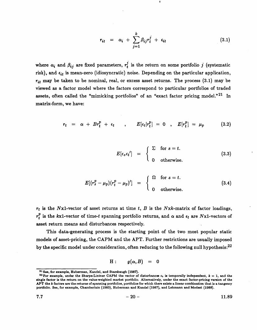
rit = <i + ZE ijr + fit (3.1)j=1

where ai and flij are fixed parameters, r is the return on some portfolio j (systematic

risk), and it is mean-zero (idiosyncratic) noise. Depending on the particular application,

rit may be taken to be nominal, real, or excess asset returns. The process (3.1) may be

viewed as a factor model where the factors correspond to particular portfolios of traded

assets, often called the "mimicking portfolios" of an "exact factor pricing model." 21 In

matrix-form, we have:

rt = a + B + Et , E[tr] = O , E[rP] = p (3.2)

E for s =t.

E [EEt'] = (3.3)El0 otherwise.

f Q for s=t.E[(r - Ap)(rP - Ap)'] = (3.4)

0 otherwise.

rt is the Nxl-vector of asset returns at time t, B is the Nxk-matrix of factor loadings,

rtp is the kxl-vector of time-t spanning portfolio returns, and a and t are Nxl-vectors of

asset return means and disturbances respectively.

This data-generating process is the starting point of the two most popular static

models of asset-pricing, the CAPM and the APT. Further restrictions are usually imposed

by the specific model under consideration, often reducing to the following null hypothesis:2 2

H: g(a,B) = o

21 See, for example, Huberman, Kandel, and Stambaugh (1987).22For example, under the Sharpe-Lintner CAPM the vector of disturbances et is temporally independent, k = 1, and the

single factor is the return on the value-weighted market portfolio. Alternatively, under the exact factor-pricing version of theAPT the k factors are the returns of spanning portfolios, portfolios for which there exists a linear combination that is a tangencyportfolio. See, for example, Chamberlain (1983), Huberman and Kandel (1987), and Lehmann and Modest (1988).

7.7 - 20 - 11.89

where the function g is model-dependent. 2 3 Many tests simply set g(a, B) = a and define

rt as excess returns, such as those of the Sharpe-Lintner CAPM and the exact factor-

pricing APT. With the added assumption that rt and r are jointly normally distributed

the finite-sample distribution of the following test statistic is well-known:

T- k-N=4' = ~ Q FN,T-k- N , (3.5)

1 + p n~ NTk-N

where E and 1 are the maximum likelihood estimators of the covariance matrices of the

disturbances t and the spanning portfolio returns r respectively, and r7 is the vector of

sample means of . If the number of available securities N is greater than the number

of time series observations T less k + 1, the estimator is singular and the test statistic

(3.5) cannot be computed without additional structure. This problem is most often cir-

cumvented in practice by forming portfolios. That is, let rt be a qxl-vector of returns of q

portfolios of securities where q < N. Since the return-generating process is linear for each

security i, a linear relation also obtains for portfolio returns. However, as the analysis of

Section 2 foreshadows, if the portfolios are constructed by sorting on some characteristic

correlated with & then the null distribution of 4' is altered.

To evaluate the null distribution of 4, under characteristic-sorting data-snooping, we

design our simulation experiments in the following way. The number of time series obser-

vations T is set to 60 for all simulations. With little loss in generality, we set the number of

spanning portfolios k to zero so that &i = T=I rit/T. To separate the effects of estimating

the covariance matrix from the effects of cross-sectional dependence, we first assume that

the covariance matrix E of t is equal to the identity matrix I - this assumption is then

relaxed in Section 3.3. We simulate T observations of the Nxl Gaussian vector rt (where

N takes the values 200, 500, and 1000), and compute &. We then form q portfolios (where

q takes the values 10 and 20) by constructing a characteristic X i that has correlation p

with &i (where p2 takes the values .01, .05, .10, .20, and .30), and then sorting the &i's by

this characteristic. To do this, we define:

Xi - + Pi , vi i.i.d. N(O, 2 = 1-p 2 (3.6)~~i =_ an 'i + Ili 17 Tp2

2 8 Examples of tests that fit into this framework are those in Campbell (1987), Connor and Korajczyk (1988), Gibbons (1982),Gibbons and Ferson (1985), Gibbons, Shanken, and Ross (1989), Huberman and Kandel (1987), MacKinlay (1987), Lehmannand Modest (1988), Stambaugh (1982), and Shanken (1985).

7.7 - 21 - 11.89

Having constructed the Xi's, we order {&i} to obtain construct portfolio intercept

estimates which we call kk, k = 1,..., n:

1n knoOk = n E c[i:N] , N - noq (3.7)

i=(k-)no+l

from which we form the F-statistic:

E = , .S-1q Fq,T.q T q, (3.8)q

where b denotes the qxl-vector of Ok's, and ] is the maximum likelihood estimator of the

qxq covariance matrix of the q portfolio returns. This procedure is repeated 5,000 times,

and the mean and standard deviation of the resulting distribution for the statistic are

reported in Table 4a, as well as the size of 1, 5, and 10 percent F-tests.

Even for as small an R 2 as 1 percent, the empirical size of the 5 percent F-test differs

significantly from its nominal value for all values of q and no. For the sample of 1,000

securities grouped into 10 portfolios, the empirical rejection rate of 36.7 percent deviates

substantially from 5 percent both economically and statistically. The size is somewhat

lower - 26.8 percent - when the 1,000 securities are grouped into 20 portfolios, matching

the pattern in Table 2a. Also similar is the monotonicity of the size with respect to

the number of securities. For 200 securities the empirical size is only 7.1 percent with 10

portfolios, but it is more than quintupled for 1,000 securities. When the squared correlation

between and Xi increases to 10 percent, the size of the F-test is essentially unity for

sample sizes of 500 or more. Thus even for finite sample sizes of practical relevance, the

importance of data-snooping via induced ordering cannot be over-emphasized.

3.3. F-Tests Without Cross-Sectional Independence.

The intuition for the substantial bias that induced ordering imparts on the size of

portfolio-based F-tests is that the induced order statistics ({&i:NJ} generally have non-

zero means; 24 hence, the average of these statistics within sorted portfolios have non-zero

24Only those &I..N for which -- will have zero expectation under the null hypothesis H.

7.7 - 22 - 11.89

means and reduced variances about those means. Alternatively, the bias from portfolio-

formation is a result of the fact that the &j's of the extreme portfolios do not approach

zero as more securities are combined, whereas the residual variances of the portfolios (and

consequently the variances of the portfolio c&'s) do tend to zero. Of course, our assumption

that the disturbances Et of (3.2) are cross-sectionally independent implies that the portfolio

residual variance approaches zero rather quickly (at rate ). But in many applications

(such as the CAPM) cross-sectional independence is too strong an assumption. Firm size

and industry membership are but two characteristics that might induce cross-sectional

correlation of security residuals. In particular, when the residuals are (positively) cross-

sectionally correlated the bias is likely to be smaller since the variance-reduction due to

portfolio-formation is less sharp than in the cross-sectionally independent case.

To provide a measure of the importance of relaxing the independence assumption,

in this section we simulate a data-generating process in which disturbances are cross-

sectionally correlated. The design is identical to that of Section 3.2 except that the residual

covariance matrix . is not diagonal. Instead, we set:

E = 66' + I (3.9)

where 6 is an Nxl vector of parameters and I is the identity matrix. Such a covariance

matrix would arise, for example, from a single common factor model .for the Nxl vector

of disturbances t:

et = 6At + vt (3.10)

where At is some i.i.d. zero-mean unit-variance common factor independent of vt, and vt

is (N-dimensional) vector white-noise with covariance matrix I. For our simulations, the

parameters 6 are chosen to be equally-spaced in the interval [-1, 1]. With this design the

cross-correlation of the disturbances will range from -0.5 to 0.5. The Xi's are constructed

as in (3.6) with:

2 (1- p2 )a 2 (ca) I 1 Np2 r2(Ca) _NT Z( + 1) (3.11)i=l

- 23 -7.7 11.89

where p2 is fixed at .05.

Under this design, the results of the simulation experiments may be compared to the

second panel of Table 4a and are reported in Table 4b.2 5 Despite the presence of cross-

sectional dependence, the impact of induced ordering on the size of the F-test is significant.

For example, with 20 portfolios each containing 25 securities the empirical size of the 5

percent test is 32.3 percent; with 10 portfolios of 50 securities each the empirical size

increases to 82.0 percent. As in the cross-sectionally independent case, the bias increases

with the number of securities given a fixed number of portfolios, and the bias decreases as

the number of portfolios is increased given a fixed number of securities. Not surprisingly,

for fixed no and q, cross-sectional dependence of the &i's lessens the bias. However, the

entries in Table 4b demonstrate that the effects of data-snooping may still be substantial

even in the presence of cross-correlation.

26 The correspondence between the two tables is not exact because the dependency introduced in (3.9) induces cross-sectionalheteroscedasticity in the &'s hence p2

= .05 yields an R2 of .05 only approximately.

7.7 - 24 - 11.89

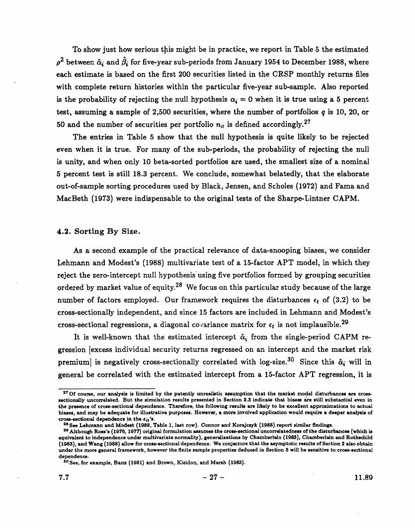
4. Two Empirical Examples.

To illustrate the potential relevance of data-snooping biases associated with induced

ordering, we provide two examples drawn from the empirical literature. The first example

is taken from the early tests of the Sharpe-Lintner CAPM, where portfolios were formed

by sorting on out-of-sample betas. We show that such tests can be biased towards falsely

rejecting the CAPM if in-sample betas are used instead, underscoring the importance of

the elaborate sorting procedures used by Black, Jensen, and Scholes (1972) and Fama

and MacBeth (1973). Our second example concerns tests of the APT that reject the zero-

intercept null hypothesis when applied to portfolio returns sorted by market value of equity.

We show that data-snooping biases can account for much the same results, and that only

additional economic restrictions will determine the ultimate source of the rejections.

4.1. Sorting By Beta.

Although tests of the Sharpe-Lintner CAPM may be conducted on individual securi-

ties, the benefits of using multiple securities is well known.2 6 One common approach for

allocating securities to portfolios has been to rank them by their betas and then group the

sorted securities. Sorting on betas essentially counteracts the Law of Large Numbers, so

that portfolios will tend to exhibit more risk dispersion than portfolios of randomly cho-

sen securities, and may therefore yield more information about the CAPM's risk-return

relation. Ideally, portfolios would be formed according to their true or population betas

However, since the population betas are unobservable, in practice portfolios have grouped

securities by their estimated betas. For example, both Black, Jensen and Scholes (1972)

and Fama and MacBeth (1973) form portfolios based on estimated betas, where the betas

are estimated with a prior sample of stock returns. Their motivation for this more com-

plicated procedure was to to avoid grouping common estimation or measurement error,

since within the sample securities with high estimated betas will tend to have positive

realizations of measurement error, and vice-versa for securities with low estimated betas.

Suppose, instead, that securities are grouped by betas estimated in-sample. Can

grouping common measurement error change inferences substantially? To answer this

question within our framework, suppose the Sharpe-Lintner CAPM obtains so that:

2 6 Blume (1970) was perhaps the first to observe that forming portfolios reduces the errors-in-variables bias in cross-sectionalregressions containing estimated betas as regressors, a problem that received considerable attention subsequently by Black,Jensen, and Scholes (1972), Fama and MacBeth (1973), and Miller and Scholes (1972).

·-- ~~- -------

11.897.7 - 25 -

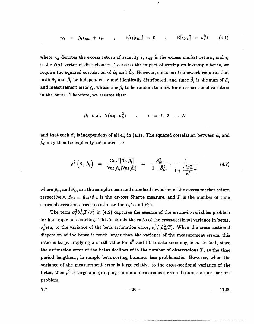
rit = Pirmt + Eit , E[Etlrmt] = 0 , E[EtEt'l] = a2I (4.1)

where rit denotes the excess return of security i, rt is the excess market return, and Et

is the Nxl vector of disturbances. To assess the impact of sorting on in-sample betas, we

require the squared correlation of &i and Pi. However, since our framework requires that

both &i and Pi be independently and identically distributed, and since fi is the sum of liand measurement error qi, we assume Pi to be random to allow for cross-sectional variation

in the betas. Therefore, we assume that:

fi i.i.d. N(AUp, c2) , i = 1, 2,..., N

and that each ,i is independent of all Ejt in (4.1). The squared correlation between ai and

Pi may then be explicitly calculated as:

(vJ (4.2)Var[&i]Var[l] 1+ srn2

where Aim and am are the sample mean and standard deviation of the excess market return

respectively, Sm- m/&m is the ez-post Sharpe measure, and T is the number of time

series observations used to estimate the ai's and li's.

The term a62 T/a2 in (4.2) captures the essence of the errors-in-variables problem

for in-sample beta-sorting. This is simply the ratio of the cross-sectional variance in betas,

ab2eta, to the variance of the beta estimation error, ua2/(2 T). When the cross-sectional

dispersion of the betas is much larger than the variance of the measurement errors, this

ratio is large, implying a small value for p2 and little data-snooping bias. In fact, since

the estimation error of the betas declines with the number of observations T, as the time

period lengthens, in-sample beta-sorting becomes less problematic. However, when the

variance of the measurement error is large relative to the cross-sectional variance of the

betas, then p2 is large and grouping common measurement errors becomes a more serious

problem.

7.7 11.89- 26 -

�___�1_______·����11___1___�_�1_*1^1__1_

Il

To show just how serious this might be in practice, we report in Table 5 the estimated

p2 between and i for five-year sub-periods from January 1954 to December 1988, where

each estimate is based on the first 200 securities listed in the CRSP monthly returns files

with complete return histories within the particular five-year sub-sample. Also reported

is the probability of rejecting the null hypothesis cai = 0 when it is true using a 5 percent

test, assuming a sample of 2,500 securities, where the number of portfolios q is 10, 20, or

50 and the number of securities per portfolio no is defined accordingly. 2 7

The entries in Table 5 show that the null hypothesis is quite likely to be rejected

even when it is true. For many of the sub-periods, the probability of rejecting the null

is unity, and when only 10 beta-sorted portfolios are used, the smallest size of a nominal

5 percent test is still 18.3 percent. We conclude, somewhat belatedly, that the elaborate

out-of-sample sorting procedures used by Black, Jensen, and Scholes (1972) and Fama and

MacBeth (1973) were indispensable to the original tests of the Sharpe-Lintner CAPM.

4.2. Sorting By Size.

As a second example of the practical relevance of data-snooping biases, we consider

Lehmann and Modest's (1988) multivariate test of a 15-factor APT model, in which they

reject the zero-intercept null hypothesis using five portfolios formed by grouping securities

ordered by market value of equity.2 8 We focus on this particular study because of the large

number of factors employed. Our framework requires the disturbances Et of (3.2) to be

cross-sectionally independent, and since 15 factors are included in Lehmann and Modest's

cross-sectional regressions, a diagonal covariance matrix for Et is not implausible. 2 9

It is well-known that the estimated intercept &i from the single-period CAPM re-

gression [excess individual security returns regressed on an intercept and the market risk

premium] is negatively cross-sectionally correlated with log-size. 3 0 Since this &j will in

general be correlated with the estimated intercept from a 15-factor APT regression, it is

2 7 0f course, our analysis is limited by the patently unrealistic assumption that the market model disturbances are cross-sectionally uncorrelated. But the simulation results presented in Section 3.3 indicate that biases are still substantial even inthe presence of cross-sectional dependence. Therefore, the following results are likely to be excellent approximations to actualbiases, and may be adequate for illustrative purposes. However, a more involved application would require a deeper analysis ofcross-sectional dependence in the eit's.

28 See Lehmann and Modest (1988, Table 1, last row). Connor and Korajczyk (1988) report similar findings.2 9 Although Ross's (1976, 1977) original formulation assumes the cross-sectional uncorrelatedness of the disturbances (which is

equivalent to independence under multivariate normality), generalizations by Chamberlain (1983), Chamberlain and Rothschild(1983), and Wang (1988) allow for cross-sectional dependence. We conjecture that the asymptotic results of Section 2 also obtainunder the more general framework, however the finite sample properties deduced in Section 3 will be sensitive to cross-sectionaldependence.

8 0 See, for example, Banz (1981) and Brown, Kleidon, and Marsh (1983).

7.7 - 27- 11.89

likely that the estimated APT-intercept and log-size will also be empirically correlated. 3 1

Unfortunately we do not have a direct measure of the correlation of the APT intercept

and log-size which is necessary to derive the appropriate null distribution after induced

ordering.3 2 As an alternative, we estimate the cross-sectional R 2 of the estimated CAPM

alpha, &i, with the logarithm of size, Xi, and we use this R 2 as well as R 2 and R 2 to

estimate the bias attributable to induced ordering.

Following Lehmann and Modest (1988), we consider four 5-year time periods from

January 1963 to December 1982. Xi is defined to be the logarithm of beginning-of-period

market values of equity. The &i's are the intercepts from regressions of excess returns on

the market risk premium as measured by the difference between an equal-weighted NYSE

index and monthly Treasury bill returns, where the NYSE index is obtained from the

Center for Research in Security Prices (CRSP) database. The R 2 's of these regressions are

reported in the second column of Table 6. One cross-sectional regression of &i on log-size

X i is run for each 5-year time period using monthly NYSE-AMEX data from CRSP. We

run regressions only for those stocks having complete return histories within the relevant

5-year period.

Table 6 contains the test statistics for a 15-factor APT framework using five size-

sorted portfolios. The first four rows contain results for each of the four sub-periods and

the last row contains aggregate test statistics. To apply the results of Sections 2 and 3

we transform Lehmann and Modest's (1988) F-statistics into (asymptotic) X2 variates. 3 3

The total number of available securities ranges from a minimum of 1001 for the first 5-year

sub-period to a maximum of 1359 for the second sub-period. For each test statistic in

Table 6 we report four different p-values: the first is with respect to the null distribution

that ignores data-snooping, and the next three are with respect to null distributions that

account for induced ordering to various degrees.

The entries in Table 6 show that the potential biases from sorting by characteristics

that have been empirically selected can be immense. The p-values range from 0.008

to 0.070 in the four sub-periods according to the standard theoretical null distribution,

yielding an aggregate p-value of 0.00014, considerable evidence against the null. When we

'1 We recognize that correlation is not transitive, so if X is correlated with Y and Y with Z, X need not be correlated withZ. However, since the intercepts from the two regressions will be functions of some common random variables, situations inwhich they are independent are the exception rather than the rule.

82 Nor did Lehmann and Modest prior to their extensive investigations. If they are subject to any data-snooping biases itis only from their awareness of size-related empirical results for the single-period CAPM, and of corresponding results for theAPT as in Chan, Chen, and Hsieh (1985).

88 Since Lehmann and Modest (1988) use weekly data the null distribution of their test statistics is Fs,2 4 0 . In practice theinferences are virtually identical using the X2 distribution after multiplying the test statistic by 5.

7.7 11.89- 28 -

adjust for the fact that the sorting characteristic is selected empirically (using the R 2 from

the cross-sectional regression of &j on Xi), the p-values for these same four sub-periods

range from 0.272 to 1.000, yielding an aggregate p-value of 1.000! Therefore, whether or

not induced ordering is allowed for can change inferences dramatically.

The appropriate R 2 in the preceding analysis is the squared correlation between log-

size and the intercept from a 15-factor APT regression, and not the one used in Table

6. To see how this may affect our conclusions, recall from 251 in Section sec25 that

the cross-sectional correlation between &j and log-size can arise from two sources: the

estimation error i in &, and the cross-sectional dispersion in the "true" CAPM aj (which

is zero under the null hypothesis). Correlation between Xi and i will be partially reflected

in correlation between the estimated APT intercept and log-size. The second source of

correlation will not be relevant under the APT null hypothesis since under that scenario

we assume that the 15-factor APT obtains and therefore the intercept vanishes for all

securities. As a conservative estimate for the appropriate R 2 to be used in Table 6, we set

the squared correlation equal to ½R2 and 1R2 , yielding the p-values reported in the last

two columns of Table 6. Even when the squared correlation is only 41?2, the inferences

change markedly after induced ordering, with p-values ranging from 0.078 to 0.720 in the

four sub-periods and 0.298 in the aggregate. This simple example illustrates the severity

with which even a mild form of data-snooping can bias our inferences in practice.

Nevertheless, it should not be inferred from Table 6 that all size-related phenomena

are spurious. After all, the correlation between X i and aj may be the result of cross-

sectional variations in the population ai's, and not estimation error. Even so, tests using

size-sorted portfolios are still biased if based on the same data from which the size effect

was previously observed. A procedure that is free from such biases is to decide today that

size is an interesting characteristic, collect ten years of new data, and then perform tests on

size-sorted portfolios from this fresh sample. If our maintained assumption (A) holds, this

will yield a perfectly valid test of the null hypothesis H since the Xi's are then independent

of the 's and induced ordering by an independent characteristic cannot disturb the null

distribution of the test statistics.

7.7 11.89- 29 -

III

5. How the Data Get Snooped.

Whether the probabilities of rejection in Table 2a are to be interpreted as size or

power depends, of course, on the particular null and alternative hypotheses at hand, the

key distinction being the source of correlation between &j and the characteristic X i. Since

our starting point in Section 2 was the assertion that this correlation is "spurious," we

view the values of Table 2a as probabilities of falsely rejecting the null hypothesis. We sug-

gested in Section sec25 that the source of this spurious correlation is correlation between

the characteristic and the estimation errors in &i, since such errors are the only source of

variation in &i under the null. But how does this correlation arise? One possibility is the

very mechanism by which characteristics are selected. Without any economic theories for

motivation, a plausible behavioral model of how we determine characteristics to be par-

ticularly "interesting" is that we tend to focus on those that have unusually large squared

sample correlations or R 2 's with the &i's. In the spirit of Ross (1987), economists study

"interesting" events, as well as events that are interesting from a theoretical perspective.

If so, then even in a collection of K characteristics all of which are independent of the

&i's, correlation between the &i's and the most "interesting" characteristic is artificially

created.

More formally, suppose for each of N securities we have a collection of K distinct

and mutually independent characteristics Yik, k = 1, 2, ... , K, where Yik is the k-th

characteristic of the i-th security. Let the null hypothesis obtain so that a i = 0 for all i,

and assume that all characteristics are independent of {&i}. This last assumption implies

that the distribution of a test statistic based on grouped '&'s is unaffected by sorting on

any of the characteristics. For simplicity let each of the characteristics and the &i 's be

normally distributed with zero mean and unit variance, and consider the sample correlation

coefficients:

k = - t=fl(Yik -Yk)( &i-) , k = 1, 2,..., K (5.1)EZ-1N_(Yik-Yk) 2 * KEN 1 (&)2

where Yk and & are the sample means of characteristic k and the &i's respectively. Suppose

we choose as our sorting characteristic the one that has the largest squared correlation with

7.7 11.89- 30 -

the &i's, and call this characteristic Xi. That is, X -Yik* where the index k* is defined

by:

A2* M .2k 1l ax- k (5.2)l<k<K

Xi is a new characteristic in the statistical sense, in that its distribution is no longer the

same as that of the Yik's.3 4 It is apparent that Xi and &i are not mutually independent

since the &i's were used in selecting this characteristic. By construction, extreme real-

izations of the random variables {Xi} tend to occur when extreme realizations of {&ij

occur.

To estimate the magnitude of correlation spuriously induced between X i and &i, first

observe that although the correlation between Yik and is zero for all k, E[,] = xunder our normality assumption. Therefore, m-1 should be our benchmark in assessing

the degree of spurious correlation between X i and &/. Since the 2 's are well-known to

be independently and identically distributed Beta(, (N - 2)) variates, the distribution

and density functions of 2k*, denoted by F(v) and f.(v) respectively, may be readily

derived as:3 5

F*(v) = [Fp(v)]K , v E (0,1) (5.3)

f*(v) = K[F(v)]'K 1ff(v) v E (0,1) (5.4)

where F and f are the c.d.f. and p.d.f. of the Beta distribution with parameters 1 and

1 (N - 2). A measure of that portion of squared correlation between Xi with &4 due to

sorting on is then given by:

'7 -E[P,]- E[pk] = f (v)d N- (5.5)

84In fact, if we denote by Yt the Nxl vector containing values of characteristic k for each of the N securities, then the vectormost highly correlated with & (which we have called X) may be viewed as the concomitant YKKI of the K-th order statistic

pK2 = Pki. As in the scalar case, induced ordering does change the distribution of the vector concomitants.saThat the squared correlation coefficients are i.i.d. Beta random variables follows from our assumptions of normality and

the mutual independence of the characteristics and the &i's (see Stuart and Ord (1987, chapter 16.28) for example). Thedistribution and density functions of the maximum follow directly from this.

�1�1_ 1_1_�_�_

7.7 - 31 - 11.89

III

For 25 securities and 50 characteristics, y is 20.5 percent! 3 6 With 100 securities, y is still

5.4 percent and only declines to 1.1 percent for N = 500. Although there is in fact no

statistical relation between any of the characteristics and the &i's, a procedure that focuses

on the most striking characteristic can create spurious statistical dependence.

As the number of securities N increases, this particular source of dependence becomes

less important since all the sample correlation coefficients Pk converge almost surely to

zero, as does y. However, recall from Table 2a that as the sample size grows the bias

increases if the number of portfolios is held fixed, hence a larger N and thus a smaller wY

does not necessarily imply a smaller bias. Moreover, since is increasing in the number of

characteristics K, we cannot find refuge in the Law of Large Numbers without weighing the

number of securities against the number of characteristics and portfolios in some fashion.

It can be argued that even the most unscrupulous investigator might hesitate at the

kind of data-snooping we have just considered. However, the very review process that

published research undergoes can have much the same effect, since competition for limited

journal space tilts the balance in favor of the most striking and dissonant of empirical re-

sults. Indeed, the "Anomalies" section of the Journal of Economic Perspectives is perhaps

the most obvious example of our deliberate search for the unusual in economics. As a con-

sequence, interest may be created in otherwise theoretically irrelevant characteristics. In

the absence of an economic paradigm, such data-snooping biases are not easily distinguish-

able from violations of the null hypothesis. This inability to separate pre-test bias from

alternative hypotheses is perhaps the most compelling criticism of "measurement without

theory."

86 Note that '- is only an approximation to the squared population correlation:

[ E(X - E[X])(& - E&]) 2/E(X- E[X]) 2

- /E(&, - E[&]) 2

However, Monte Carlo simulations ~with 10,000 replications show that this approximation is excellent even for small samplesizes. For example, fixing K at 50, the correlation from the simulations is 22.82 percent for N = 25, whereas (5.5) yields'- = 20.47 percent; for N = 100 the simulations yield a correlation of 6.25 percent, compared to a of 5.39 percent.

7.7 - 32 - 11.89

___l__l______ll__�_rr__ 1_.. .I�XI--l.l�n�-X�·I�*�1·_�*____

6. Conclusion.

Although the size effect may signal important differences between the economic struc-

ture of small and large corporations, how these differences are manifested in the stochastic

properties of their equity returns cannot be reliably determined purely through data anal-

ysis. Much more convincing would be the empirical significance of size, or any other

quantity, that is based on a model of economic equilibrium in which the characteristic is

shown to be related to the behavior of asset returns. Our findings show that tests using

securities grouped according to theoretically-motivated correlations between X i and &i can

be powerful indeed. Interestingly, tests of the APT with portfolios sorted by such charac-

teristics (own-variance and dividend yield) no longer reject the null hypothesis. 3 7 Sorting

on size yields rejections whereas sorting on theoretically relevant characteristics such as

own-variance and dividend yield does not. This suggests that data-motivated grouping

procedures should be employed cautiously.

It is widely acknowledged that incorrect conclusions may be drawn from procedures

violating the assumptions of classical statistical inference, but the nature of these violations

is often as subtle as it is profound. In observing that economists (as well as those in the

natural sciences) tend to seek out anomalies, Merton (1988, p.104) writes: "All this fits

well with what the cognitive psychologists tell us is our natural individual predilection to

focus, often disproportionately so, on the unusual. .... This focus, both individually and

institutionally, together with little control over the number of tests performed, creates a

fertile environment for both unintended selection bias and for attaching greater significance

to otherwise unbiased estimates than is justified." The recognition of this possibility is

a first step in guarding against it. The results of our paper provide a more concrete

remedy for such biases in the particular case of portfolio formation via induced ordering

on data-instigated characteristics. However, non-experimental inference may never be

completely free from data-snooping biases since the attention given to empirical anomalies,

incongruities, and unusual correlations is also the modus operandi for genuine discovery

and progress in the social sciences. Formal statistical analyses such as ours may serve

as primitive guides to a better understanding of economic phenomena, but the ability to

distinguish between the spurious and the substantive is likely to remain a cherished art.

s7See Lehmann and Modest (1988). Chen, Roll, and Ross (1986, footnote 8) report similar negative findings for the APTwith portfolios formed by sorting on CAPM betas, the standard deviation of returns in a market-model regression, and thelevel of the stock price.

� _rl ___

7.7 - 33- 11.89

References

Aldous, D., 1989, Probability Approximations via the Poisson Clumping Heuristic, NewYork: Springer-Verlag.

Banz, R. W., 1981, The Relationship Between Return and Market Value of CommonStocks," Journal of Financial Economics 9, 3-18.

Berger, J. and R. Wolpert, The Likelihood Principle, Lecture Notes - Monograph SeriesVolume 6, Hayward: Institute of Mathematical Statistics.

Bhattacharya, P. K., 1974, Convergence of Sample Paths of Normalized Sums of InducedOrder Statistics," Annals of Statistics 2, 1034-1039.

, 1984, "Induced Order Statistics: Theory and Applications," in P. R. Krishnaiahand P. K. Sen (eds.) Handbook of Statistics 4: Nonparametric Methods, Amsterdam:North-Holland.

Black, F., Jensen, M., and M. Scholes, 1972, "The Capital Asset Pricing Model: SomeEmpirical Tests," in M. Jensen (ed.) Studies in the Theory of Capital Markets, NewYork: Praeger.

Blume, M., 1970, "Portfolio Theory: A Step Towards Its Practical Application," Journalof Business 43, 152-173.

Brown, P., Kleidon, A. and T. Marsh, 1983, "New Evidence on the Nature of Size RelatedAnomalies in Stock Prices," Journal of Financial Economics 12, 33-56.

Campbell, J. Y., 1987, "Stock Returns and the Term Structure," Journal of FinancialEconomics 18, 373-400.

Chamberlain, G., 1983, "Funds, Factors, and Diversification in Arbitrage Pricing Models,"Econometrica 51, 1305-1323.

, and M. Rothschild, 1983, Arbitrage, Factor Structure, and Mean-Variance Anal-ysis on Large Asset Markets," Fconometrica 51, 1281-1304.

Chan, K. and N. Chen, 1988, An Unconditional Asset-Pricing Test and the Role of FirmSize as an Instrumental Variable for Risk," Journal of Finance 43, 309-325.

, and D. Hsieh, 1985, "An Exploratory Investigation of the Firm Size Effect," Jour-nal of Financial Economics 14, 451-471.

Chen, N., Roll, R. and S. Ross, 1986, "Economic Forces and the Stock Market," Journalof Business 59, 383-403.

Connor, G. and R. Korajczyk, 1988, Risk and Return in an Equilibrium APT: Applicationof a New Test Methodology," Journal of Financial Economics 21, 255-290.

David, H. A., 1973, Concomitants of Order Statistics," Bulletin of the InternationalStatistical Institute 45, 295-300.

, 1981, Order Statistics, Second Edition, New York: John Wiley and Sons.

7.7 11.89- 34 -

III

~--, and J. Galambos, 1974, UThe Asymptotic Theory of Concomitants of Order Statis-tics," Journal of Applied Probability 11, 762-770.

-- , O'Connell, M. J. and S. S. Yang, 1977, Distribution and Expected Value of theRank of a Concomitant of an Order Statistic," Annals of Statistics 5, 216-223.

Fama, E. and J. MacBeth, 1973, "Risk, Return, and Equilibrium: Empirical Tests," Jour-nal of Political Economy 71, 607-636.

Galambos, J., 1987, The Asymptotic Theory of Extreme Order Statistics, Second Edition,Malabar: Krieger Publishing Company.

Gibbons, M. R., 1982, "Multivariate Tests of Financial Models: A New Approach," Journalof Financial Economics 10, 3-27.

~- -- , and W. Ferson, 1985, "Testing Asset Pricing Models With Changing Expectationsand an Unobservable Market Portfolio," Journal of Financial Economics 14, 217-236.

- , Ross, S. A. and J. Shanken, 1989, "A Test of the Efficiency of a Given Portfolio,"Econometrica 57, 1121-1152.

Huberman, G. and S. Kandel, 1987, "Mean Variance Spanning," Journal of Finance 42,873-888.

Huberman, G. Kandel, S. and R. Stambaugh, 1987, "Mimicking Portfolios and ExactArbitrage Pricing," Journal of Finance 42, 1-10.

Iyengar, S. and J. Greenhouse, 1988, Selection Models and the File Drawer Problem,"Statistical Science 3, 109-135.

Kandel, S. and R. Stambaugh, 1987, "On Correlations and Inferences About Mean-VarianceEfficiency," Journal of Financial Economics 18, 61-90.

Lakonishok, J. and S. Smidt, 1988, "Are Seasonal Anomalies Real? A Ninety-Year Per-spective," Review of Financial Studies 1, 403-426.

Leamer, E., 1978, Specification Searches, New York: John Wiley and Sons.

Lehmann, B. N. and D. Modest, 1988, "The Empirical Foundations of the Arbitrage PricingTheory," Journal of Financial Economics 21, 213-254.

MacKinlay, A. C., 1987, "On Multivariate Tests of the CAPM," Journal of FinancialEconomics 18, 341-372.

Merton, R., 1987, "On the Current State of the Stock Market Rationality Hypothesis," inR. Dornbusch, S. Fischer, and J. Bossons (eds.), Macroeconomics and Finance: Essaysin Honor of Franco Modigliani, Cambridge: M.I.T. Press.

Nagaraja, H. N., 1982a, "Some Asymptotic Results for the Induced Selection Differential,"Journal of Applied Probability 19, 233-239.

, 1982b, "Some Nondegenerate Limit Laws for the Selection Differential," Annalsof Statistics 10, 1306-1310.

, 1984, "Some Nondegenerate Limit Laws for Sample Selection Differential AndSelection Differential," Sankhyd 46, Series A, 355-369.

- 35 -

_ _I�__

7.7 11.89

III

Ross, S., 1987, "Regression to the Max," Working Paper, Yale School of Organization andManagement.

Sandstr6m, A., 1987, "Asymptotic Normality of Linear Functions of Concomitants of OrderStatistics," Metrika 34, 129-142.

Sen, P. K., 1976, A Note On Invariance Principles For Induced Order Statistics," Annalsof Probability 4, 474-479.

, 1981, "Some Invariance Principles for Mixed Rank Statistics and Induced OrderStatistics and Some Applications," Communications in Statistics A10, 1691-1718.

Shanken, J., 1985, "Multivariate Tests of the Zero-Beta CAPM," Journal of FinancialEconomics 14, 327-348.

Siegmund, D., 1985, Sequential Analysis, New York: Springer-Verlag.

Stalabaugh, R. F., 1982, "On the Exclusion of Assets from Tests of the Two ParameterModel," Journal of Financial Economics 10, 235-268.

Stuart, A. and J. Ord, 1987, Kendall's Advanced Theory of Statistics, New York: OxfordUniversity Press.

Wald, A., 1947, Sequential Analysis, New York: John Wiley and Sons.

Wang, T., 1988, Essays on the Theory of Arbitrage Pricing, unpublished doctoral disser-tation, Wharton School, University of Pennsylvania.

Watterson, G. A., 1959, "Linear Estimation in Censored Samples from Multivariate NormalPopulations," Annals of Mathematical Statistics 30, 814-824.

Yang, S. S., 1977, "General Distribution Theory of the Concomitants of Order Statistics,"Annals of Statistics 5, 996-1002.

, 1981a, "Linear Functions of Concomitants of Order Statistics With Applicationto Nonparametric Estimation of a Regression Function," Journal of the American Sta-tistical Association 76, 658-662.

1981b, "Linear Combinations of Concomitants of Order Statistics with Applicationto Testing and Estimation," Annals of the Institute of Statistical Mathematics 33 (PartA), 463-470.

7.7 - 36 - 11.89

� �^`�����11�1"`--��`"l�`���'l ~ �`� ~�; �-- -��1"��'������-�c-�"""I ����-"-^^������~��'���"`�-�I-i-------

Table 1

Theoretical sizes of nominal 5 percent X -tests of H: ai = 0 (i = 1,...,n) using the test statistics i, where ,j _

I=1 &2; ():N/'/02, j = 1, 2, 3 for various sample sizes n. The statistic i1 is based on induced order statistics with relative

ranks evenly spaced in (0,1); °2 is constructed from induced order statistics ranked in the lowest and highest 100/(m+ 1)-percentfractiles; and is is constructed from those ranked in the second lowest and second highest 100/(m + 1)-percent fractiles. TheR2 is the square of the correlation between &i and the sorting characteristic.

n il-Test 02-Test is-Test 92-Test 8s-Test h2-Test is-Test(m = 4) (m = 4) (m = 9) (m = 9) (m = 19) (m = 19)

R2

= .01

10 0.049 0.053 0.048 0.056 0.050 0.059 0.05320 0.049 0.054 0.047 0.058 0.050 0.063 0.05450 0.049 0.056 0.046 0.063 0.051 0.071 0.057100 0.049 0.059 0.045 0.069 0.051 0.081 0.059

R2 = .05

10 0.045 0.063 0.041 0.080 0.051 0.101 0.06620 0.045 0.070 0.038 0.096 0.052 0.130 0.07350 0.046 0.086 0.033 0.135 0.053 0.201 0.087100 0.047 0.107 0.028 0.190 0.054 0.304 0.106

R2 = .10

10 0.040 0.076 0.032 0.116 0.052 0.166 0.08320 0.041 0.093 0.028 0.158 0.053 0.244 0.09950 0.042 0.133 0.020 0.267 0.055 0.442 0.137100 0.043 0.192 0.014 0.423 0.058 0.680 0.191

R2 = .20

10 0.030 0.104 0.019 0.202 0.052 0.330 0.12120 0.032 0.146 0.013 0.318 0.054 0.528 0.16350 0.034 0.262 0.006 0.599 0.059 0.862 0.272100 0.036 0.432 0.002 0.857 0.064 0.987 0.429

R2 = .30

10 0.021 0.134 0.010 0.307 0.050 0.520 0.16320 0.023 0.212 0.005 0.511 0.053 0.786 0.24250 0.026 0.428 0.001 0.863 0.060 0.989 0.447100 0.029 0.696 0.000 0.989 0.069 1.000 0.692

7.2.1 2.89

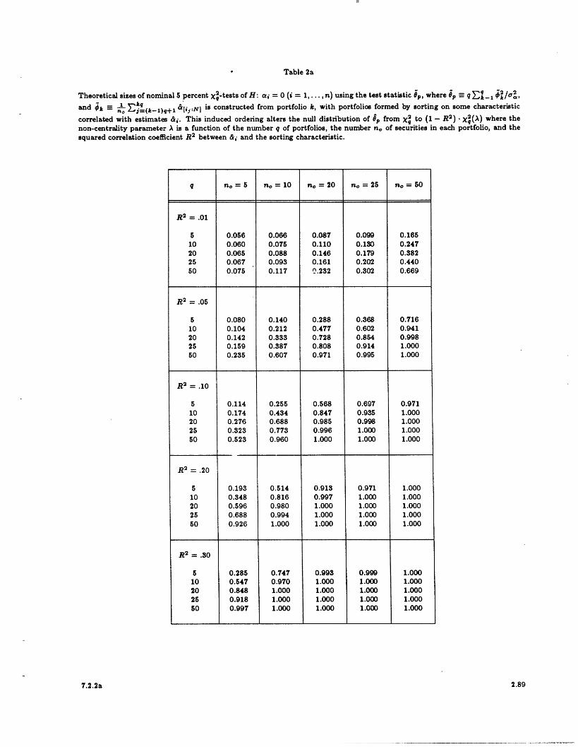
III

Table 2a

Theoretical sizes of nominal 5 percent X2-tests of H: a; = 0 (i = 1 , n) using the test statistic ip, where 6p q _l ~ ° 2

and n o _ $=_(k--1)q+l &li[j:N is constructed from portfolio k, with portfolios formed by sorting on some characteristic

correlated with estimates &;. This induced ordering alters the null distribution of 9p from X to (1 - R2 ) X(A) where thenon-centrality parameter A is a function of the number q of portfolios, the number no of securities in each portfolio, and thesquared correlation coefficient R2 between &i and the sorting characteristic.

7.2.2a

q no = 5 no = 10 no = 20 no = 25 no = 50

R2 = .01

5 0.056 0.066 0.087 0.099 0.16510 0.060 0.075 0.110 0.130 0.24720 0.065 0.088 0.146 0.179 0.38225 0.067 0.093 0.161 0.202 0.44050 0.075 0.117 0.232 0.302 0.669

// = .05

5 0.080 0.140 0.288 0.368 0.71610 0.104 0.212 0.477 0.602 0.94120 0.142 0.333 0.728 0.854 0.99825 0.159 0.387 0.808 0.914 1.00050 0.235 0.607 0.971 0.995 1.000

R = .10

5 0.114 0.255 0.568 0.697 0.97110 0.174 0.434 0.847 0.935 1.00020 0.276 0.688 0.985 0.998 1.00025 0.323 0.773 0.996 1.000 1.00050 0.523 0.960 1.000 1.000 1.000

R2 = .20

5 0.193 0.514 0.913 0.971 1.00010 0.348 0.816 0.997 1.000 1.00020 0.596 0.980 1.000 1.000 1.00025 0.688 0.994 1.000 1.000 1.00050 0.926 1.000 1.000 1.000 1.000

R2 = .30

5 0.285 0.747 0.993 0.999 1.00010 0.547 0.970 1.000 1.000 1.00020 0.848 1.000 1.000 1.000 1.00025 0.918 1.000 1.000 1.000 1.00050 0.997 1.000 1.000 1.000 1.000

2.89

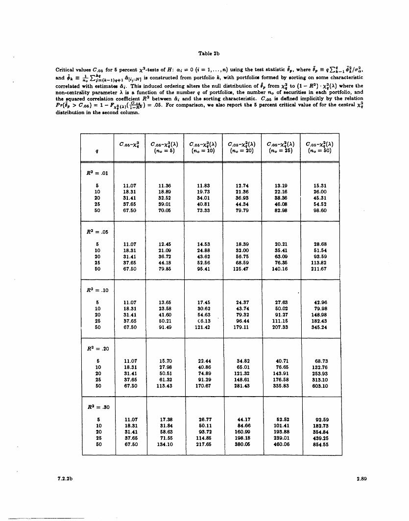
Table 2b

Critical values C.os for 5 percent X2 -tests of H: ai = 0 (i = 1,...,n) using the test statistic Op, where p qrk- i/ c,

and ~k- no j=(-l)q+l &[ij.N] is constructed from portfolio k, with portfolios formed by sorting on some characteristic

correlated with estimates &i. This induced ordering alters the null distribution of av from X2 to (1 - R2 ) X2(A) where thenon-centrality parameter A is a function of the number q of portfolios, the number no of securities in each portfolio, andthe squared correlation coefficient R2 between &i and the sorting characteristic. C.os is defined implicitly by the relationPr(Op > C.0 6 ) = 1 - Fx ()( f) = .05. For comparison, we also report the 5 percent critical value of for the central X2

distribution in the second column.

q (no = 5) (no = 10) (no = 20) (no = 25) (no = 50)

R2 = .01

5 11.07 11.36 11.83 12.74 13.19 15.3110 18.31 18.89 19.73 21.36 22.16 26.0020 31.41 32.52 34.01 36.93 38.36 45.3125 37.65 39.01 40.81 44.34 46.08 54.5250 67.50 70.05 73.33 79.79 82.98 98.60

R2 = .05

5 11.07 12.45 14.53 18.39 20.21 28.6810 18.31 21.09 24.88 32.00 35.41 51.5420 31.41 36.72 43.62 56.75 63.09 93.5925 37.65 44.18 52.56 68.59 76.35 113.8250 67.50 79.85 95.41 125.47 140.16 211.67

R2 = .10

5 11.07 13.65 17.45 24.37 27.63 42.9610 18.31 23.58 30.62 43.74 50.02 79.9820 31.41 41.60 54.63 79.32 91.27 148.9825 37.65 50.21 £6.13 96.44 111.15 182.4350 67.50 91.49 121.42 179.11 207.33 345.24

R2

= .20

5 11.07 15.70 22.44 34.82 40.71 68.7310 18.31 27.98 40.86 65.01 76.65 132.7620 31.41 50.51 74.89 121.32 143.91 253.9325 37.65 61.32 91.29 148.61 176.58 313.1050 67.50 113.43 170.67 281.43 335.83 603.10

R2 = .30

5 11.07 17.38 26.77 44.17 52.52 92.5910 18.31 31.84 50.11 84.66 101.41 182.7320 31.41 58.63 93.72 160.99 193.88 354.8425 37.65 71.55 114.85 198.18 239.01 439.2550 67.50 134.10 217.65 380.05 460.06 854.55

7.2.2b 2.89

11

Table 3

Empirical sizes of nominal 5 percent X~-tests of H: ai = 0 (i = 1,...,n) using the test statistic 7p, where ~p - qI-q 1k '2=

and h -= no ~i=(k-1)q+l &lijNl is constructed from portfolio k, with portfolios formed by sorting on some characteristic

correlated with estimates ai. This induced ordering alters the null distribution of 6p from X to (1- R2 ) X2(A) where thenon-centrality parameter A is a function of the number q of portfolios, the number no of securities in each portfolio, and thesquared correlation coefficient R2 between &i and the sorting characteristic. Each simulation is based on 5,000 replications;asymptotic standard errors for the size estimates may be obtained from the usual binomial approximation, and is 3.08 x 10-3for the 5 percent test.

7.2.3

q no = 5 n = 10 no = 20 no = 25 no = 50

R2=.01

5 0.058 0.064 0.093 0.105 0.17410 0.059 0.076 0.119 0.130 0.25720 0.057 0.083 0.140 0.188 0.38525 0.069 0.100 0.170 0.206 0.44550 0.083 0.118 0.244 0.300 0.679

R2 = .05

5 0.091 0.149 0.310 0.392 0.72310 0.117 0.227 0.493 0.611 0.94320 0.156 0.351 0.744 0.854 0.99925 0.163 0.401 0.818 0.916 1.00050 0.249 0.616 0.971 0.997 1.000

R = .10

5 0.141 0.285 0.601 0.721 0.97310 0.197 0.473 0.854 0.937 1.00020 0.308 0.709 0.985 0.998 1.00025 0.338 0.789 0.995 1.000 1.00050 0.545 0.961 1.000 1.000 1.000

R2 = .20

5 0.267 0.577 0.922 0.974 1.00010 0.405 0.833 0.997 1.000 1.00020 0.635 0.982 1.000 1.000 1.00025 0.728 0.996 1.000 1.000 1.00050 0.933 1.000 1.000 1.000 1.000

R2= .30

5 0.388 0.790 0.992 1.000 1.00010 0.620 0.971 1.000 1.000 1.00020 0.868 1.000 1.000 1.000 1.00025 0.922 1.000 1.000 1.000 1.00050 0.997 1.000 1.000 1.000 1.000

2.89

Table 4a

Empirical size of Fq,T-g tests based on q portfolios sorted by a random characteristic whose squared correlation with &ii isR2. n is the number of securities in each portfolio and n nq is the total number of securities. The number of time seriesobservations T is set to 60. The mean and standard deviation of the test statistic over the 5,000 replications are reported. Thepopulation mean and standard deviation of Flo,so are 1.042 and 0.523 respectively; those of the F2o, 4o are 1.053 and 0.423respectively. Asymptotic standard errors for the size estimates may be obtained from the usual binomial approximation; theyare 4.24 x 10-3, 3.08 x 10 - S , and 1.41 x 10-3 for the 10, 5, and 1 percent tests respectively.

q no n Mean Std. Dev. Size-10% Size-S% Size-l%

R2 = .01

10 20 200 1.225 0.619 0.181 0.071 0.02620 10 200 1.148 0.460 0.148 0.079 0.01810 50 500 1.512 0.728 0.318 0.152 0.07020 25 500 1.301 0.514 0.240 0.143 0.03610 100 1000 '2.030 0.908 0.576 0.367 0.20320 50 1000 1.554 0.596 0.405 0.268 0.098

R2

= .05

10 20 200 1.980 0.883 0.549 0.342 0.18920 10 200 1.505 0.582 0.369 0.241 0.08210 50 500 3.501 1.335 0.945 0.846 0.70020 25 500 2.264 0.801 0.798 0.670 0.38210 100 1000 5.991 1.976 0.999 0.997 0.98620 50 1000 3.587 1.169 0.992 0.972 0.879

R2 = .10

10 20 200 2.961 1.196 0.868 0.713 0.53820 10 200 1.977 0.727 0.658 0.510 0.25710 50 500 6.939 1.931 0.999 0.997 0.98720 25 500 3.526 1.128 0.988 0.968 0.86810 100 1000 10.888 3.050 1.000 1.000 1.00020 50 1000 6.123 1.811 1.000 1.000 0.999

R2 = .20

10 20 200 4.831 1.657 0.997 0.982 0.93720 10 200 2.895 0.992 0.948 0.882 0.66710 50 500 10.796 3.022 1.000 1.000 1.00020 25 500 6.005 1.758 1.000 1.000 0.99810 100 1000 20.695 5.112 1.000 1.000 1.00020 60 1000 11.194 2.988 1.000 1.000 1.000

R2 = .30

10 20 200 6.710 2.119 1.000 0.999 0.99720 10 200 3.841 1.204 0.996 0.987 0.92810 50 500 15.619 3.996 1.000 1.000 1.00020 25 500 8.535 2.366 1.000 1.000 1.00010 100 1000 30.671 7.156 1.000 1.000 1.00020 50 1000 16.183 4.112 1.000 1.000 1.000

7.2.4a

." ~-~-- -

2.89

Table 4b

Empirical size of Fq,T-q tests based on q portfolios sorted by a random characteristic whose squared correlation with &i isapproximately .05. no is the number of securities in each portfolio and n noq is the total number of securities. The &i's of theportfolios are cross-sectionally correlated, where the source of correlation is an i.i.d. zero-mean common factor in the returns.The number of time series observations T is set to 60. The mean and standard deviation of the test statistic over the 5,000replications are reported. The population mean and standard deviation of F1o,1o are 1.042 and 0.523 respectively; those ofthe F20 ,4o are 1.053 and 0.423 respectively. Asymptotic standard errors for the size estimates may be obtained from the usualbinomial approximation; they are 4.24 x 10- 3 , 3.08 x 10- S, and 1.41 x 10- 3 for the 10, 5, and 1 percent tests respectively.

7.2.4b

q no n | Mean Std. Dev. Size-10% Size-5% Size-1%

R2 .05

10 20 200 1.700 0.763 0.422 0.216 0.10020 10 200 1.372 0.528 0.270 0.167 0.047

10 50 500 2.520 1.041 0.765 0.565 0.36720 25 500 1.867 0.693 0.593 0.322 0.205

10 100 1000 3.624 1.605 0.925 0.820 0.68220 50 1000 2.516 0.966 0.844 0.743 0.501

-- I-��-������-�"~"~"""�~"~�""~�""�"""""

"I

2.89

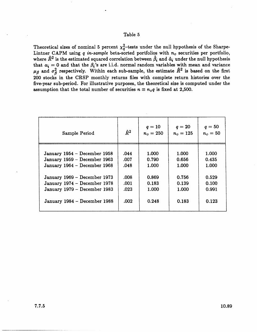
Table 5

Theoretical sizes of nominal 5 percent X2-tests under the null hypothesis of the Sharpe-Lintner CAPM using q in-sample beta-sorted portfolios with no securities per portfolio,where / 2 is the estimated squared correlation between /i and &j under the null hypothesisthat ai = 0 and that the i's are i.i.d. normal random variables with mean and variancepi and ok respectively. Within each sub-sample, the estimate R 2 is based on the first200 stocks in the CRSP monthly returns files with complete return histories over thefive-year sub-period. For illustrative purposes, the theoretical size is computed under theassumption that the total number of securities n- noq is fixed at 2,500.

10.89

q = 10 q = 20 q =50Sample Period /2 no = 250 no = 125 no = 50

January 1954 - December 1958 .044 1.000 1.000 1.000January 1959 - December 1963 .007 0.790 0.656 0.435January 1964 - December 1968 .048 1.000 1.000 1.000

January 1969 - December 1973 .008 0.869 0.756 0.529January 1974 - December 1978 .001 0.183 0.139 0.100January 1979 - December 1983 .023 1.000 1.000 0.991

January 1984 - December 1988 .002 0.248 0.183 0.123

7.7.5

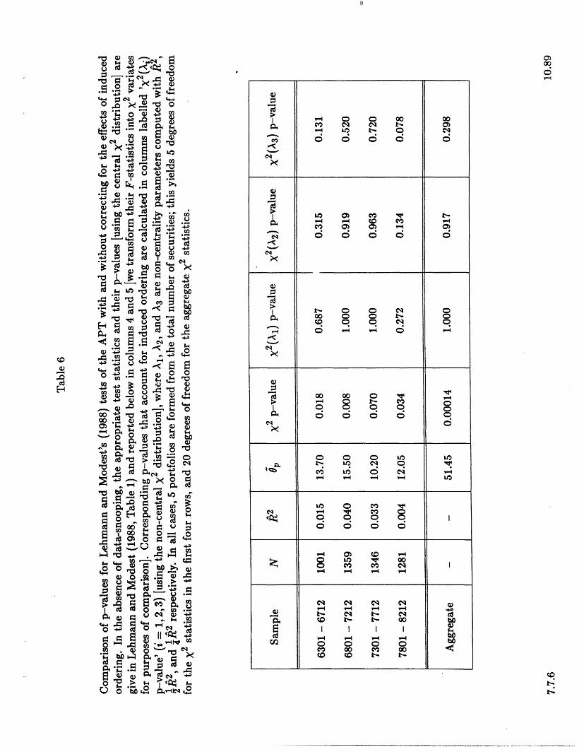
4 - 4) 4 o

>0 > o0 0 0~ .

O . ' '

4- 0 II '-

a A-< .

w * 0"4-1MI '4 ,0 2 .

b h rie0 4

4.0(`'S~

00. I o o o o oI 00 0 0 00 0- I

eq

cx I

00 0 0 -O0 - d c 4-

0 0D 0 0t | o 8 8 0 0r.o o 0 0 oe o o

zY 0

CE0 e~03~~~~ k3-t0

oo00

111