business-cycle anatomy - mit economics
TRANSCRIPT

American Economic Review 2020, 110(10): 3030–3070 https://doi.org/10.1257/aer.20181174
3030
Business-Cycle Anatomy†
By George-Marios Angeletos, Fabrice Collard, and Harris Dellas*
We propose a new strategy for dissecting the macroeconomic time series, provide a template for the business-cycle propagation mech-anism that best describes the data, and use its properties to appraise models of both the parsimonious and the medium-scale variety. Our findings support the existence of a main business-cycle driver but rule out the following candidates for this role: technology or other shocks that map to TFP movements; news about future productivity; and inflationary demand shocks of the textbook type. Models aimed at accommodating demand-driven cycles without a strict reliance on nominal rigidity appear promising. (JEL C22, E10, E32)
One is led by the facts to conclude that, with respect to the qualitative behavior of comovements among series, business cycles are all alike. To theoretically inclined economists, this conclusion should be attractive and challenging, for it suggests the possibility of a unified explanation of busi-ness cycles.
—Lucas (1977)
In their quest to explain macroeconomic fluctuations, macroeconomists have often relied on models in which a single, recurrent shock acts as the main business-cycle driver.1 This practice is grounded not only on the desire to offer a parsimonious, unifying explanation as suggested by Lucas, but also on the prop-erty that such a model may capture diverse business-cycle triggers if these share a common propagation mechanism: multiple shocks that produce similar impulse
1 Examples include the monetary shock in Lucas (1975), the TFP shock in Kydland and Prescott (1982), the sunspot in Benhabib and Farmer (1994), the investment shock in Justiniano, Primiceri, and Tambalotti (2010), the risk shock in Christiano, Motto, and Rostagno (2014), and the confidence shock in Angeletos, Collard, and Dellas (2018).
* Angeletos: MIT Department of Economics (email: [email protected]); Collard: Toulouse School of Economics (CNRS) (email: fabrice.collard@ tse-fr.eu); Dellas: Department of Economics, University of Bern (email: [email protected]). Mikhail Golosov was the coeditor for this article. A preliminary version of the empirical strategy of this paper appeared in Section II of Angeletos, Collard, and Dellas (2015); this earlier exploration is fully subsumed here. We thank the coeditor, Mikhail Golosov, and three anonymous referees for extensive feed-back. For useful comments, we also thank Fabio Canova, Larry Christiano, Patrick Fève, Francesco Furlanetto, Jordi Galí, Lars Hansen, Franck Portier, Juan Rubio-Ramirez, and participants at various seminars and conferences. Angeletos acknowledges the financial support of the National Science Foundation (Award #1757198). Collard acknowledges funding from the French National Research Agency (ANR) under the Investments for the Future program (Investissements d’Avenir, grant ANR-17-EURE-0010).
† Go to https://doi.org/10.1257/aer.20181174 to visit the article page for additional materials and author disclosure statements.
3031ANGELETOS ET AL.: BUSINESS-CYCLE ANATOMYVOL. 110 NO. 10
responses for all variables of interest can be considered as essentially the same shock.2
Is there evidence of such a common propagation mechanism in macroeconomic data? And if yes, what does it look like?
We address these questions with the help of a new empirical strategy. The strat-egy involves taking multiple cuts of the data. Each cut corresponds to a structural vector autoregression (SVAR)-based shock that accounts for the maximal volatility of a particular variable over a particular frequency band. Whether these empirical objects have a true structural counterpart in the theory or not, their properties form a rich set of cross-variable, static and dynamic restrictions, which can inform macro-economic theory. We call this set the “anatomy.”
A core subset of the anatomy is the collection of the five shocks obtained by targeting the main macroeconomic quantities, namely unemployment, output, hours worked, consumption, and investment, over the business-cycle frequencies. These shocks turn out to be interchangeable in the sense of giving rise to nearly the same impulse response functions (IRFs) for all the variables, as well as being highly cor-related with one another.
The interchangeability of these empirical shocks supports parsimonious theories featuring a main, unifying, propagation mechanism. Their shared IRFs provide an empirical template of it.
In combination with other elements of our anatomy, this template rules out the following candidates for the main driver of the business cycle: technology or other shocks that map to TFP movements; news about future productivity; and inflation-ary demand shocks of the textbook type.
Prominent members of the dynamic stochastic general equilibrium (DSGE) liter-ature also lack the propagation mechanism seen in our anatomy of the data, despite their use of multiple shocks and flat Phillips curves and their good fit in other dimen-sions. The problem seems to lie in the flexible-price core of these models. Models that instead allow for demand-driven cycles without a strict reliance on nominal rigidity hold promise.3
A. The Empirical Strategy
We first estimate a VAR (or a vector error correction model (VECM)) on the fol-lowing ten macroeconomic variables over the 1955–2017 period: the unemployment rate; the per capita levels of GDP, investment (inclusive of consumer durables), consumption (of nondurables and services), and total hours worked; labor produc-tivity in the nonfarm business sector; utilization-adjusted total factor productivity (TFP); the labor share; the inflation rate (GDP deflator); and the federal funds rate. We next compile a collection of shocks, each of which is identified by maximizing
2 To echo Cochrane (1994, p. 298): “The study of shocks and propagation mechanisms are of course not sepa-rate enterprises. Shocks are only visible if we specify something about how they propagate to observable variables.”
3 Recent examples include Angeletos, Collard, and Dellas (2018); Angeletos and La’O (2010, 2013); Angeletos and Lian (2020); Bai, Ríos-Rull, and Storesletten (2017); Beaudry and Portier (2014, 2018); Beaudry, Galizia, and Portier (2018); Benhabib, Wang, and Wen (2015); Eusepi and Preston (2015); Huo and Rios-Rull (forthcoming) ;Jaimovich and Rebelo (2009); Huo and Takayama (2015); and Ilut and Saijo (2018). Related is also the earlier literature on coordination failures (Diamond 1982, Benhabib and Farmer 1994, Guesnerie and Woodford 1993).

3032 THE AMERICAN ECONOMIC REVIEW OCTOBER 2020
its contribution to the volatility of a particular variable over either business-cycle frequencies ( 6–32 quarters) or long-run frequencies (80– ∞ ). We finally inspect the empirical patterns encapsulated in each of these shocks, namely the implied IRFs and variance contributions.
This approach builds on the important work of Uhlig (2003). Our main contri-bution vis-à-vis this and other works that employ the so-called max-share identifi-cation strategy (Barsky and Sims 2011, Faust 1998, Neville et al. 2014) lies in the multitude of the one-dimensional cuts of the data considered, the empirical regular-ities thus recovered, and the novel lessons drawn for theory.4
An additional contribution is to clarify the mapping from the frequency domain to the time domain: we show that the shock that dominates the business-cycle fre-quencies ( 6–32 quarters) is a shock whose footprint in the time domain peaks within a year or two. In other words, targeting 6–32 quarters in the time domain does not recover the business cycle.
Our approach also departs from standard practice in the SVAR literature, which aims at identifying empirical counterparts to specific theoretical shocks (for a review, see Ramey 2016). Instead, it sheds light on dynamic comovements by tak-ing multiple cuts of the data, one per targeted variable and frequency band. These multiple cuts form a rich set of empirical restrictions that can discipline any theory, whether of the parsimonious type or the DSGE type.
B. The Main Business-Cycle Shock
Consider the shocks that target any of the following variables over the business-cycle frequencies: unemployment, hours worked, GDP, and investment. These shocks are interchangeable in terms of the dynamic comovements, or the IRFs, they produce. Furthermore, any one of them accounts for about three-quarters of the business-cycle volatility of the targeted variable and for more than one-half of the business-cycle volatility in the remaining variables, and also triggers strong positive comovement in all variables. In expanded specifications that include the output gap or the unemployment gap, the shocks identified by targeting any one of these gaps produce nearly identical patterns as well. Finally, the shock that targets consumption is less tightly connected in terms of variance contributions, but still similar in terms of dynamic comovements.
These findings offer support for theories featuring either a single, dominant, business-cycle shock, or multiple shocks that leave the same footprint because they share the same propagation mechanism. With this idea in mind, we use the term Main Business Cycle (MBC) shock to refer to the common empirical footprint, in terms of IRFs, of the aforementioned reduced-forms shocks. This provides the sought-after template for what the propagation mechanism should be in any “good” model of the business cycle.5
4 A detailed discussion of how our method and results differ from those of Uhlig (2003) and various other works is offered in the next section.
5 As with any other filter that focuses on the business-cycle frequencies of the data, the use of our template for model evaluation is of course based on the premise that business-cycle models ought to be evaluated by such a met-ric. This accords with a long tradition in macroeconomics. See, however, Canova (2020) for a contrarian view based on the property that the business-cycle and lower-frequency predictions of DSGE models are tightly tied together;
3033ANGELETOS ET AL.: BUSINESS-CYCLE ANATOMYVOL. 110 NO. 10
A central feature of this template is the interchangeability property, namely that all the aforementioned shocks produce essentially the same IRFs, or the same prop-agation mechanism. Below, we describe additional stylized facts revealed via our anatomy and discuss the overall lessons for theory. At first, we draw lessons through the perspective of single-shock models. Later, we switch to multishock models and discuss the challenges and the use of our method in such models.
C. Disconnect from TFP and from the Long Run
The MBC shock is disconnected from TFP at all frequencies. It also accounts for little of the long-term variation in output, investment, consumption, and labor pro-ductivity. Symmetrically, the shocks that have the maximal contribution to long-run volatility have a small contribution to the business cycle.
These findings challenge not only the baseline RBC model but also models that map other shocks, including financial, uncertainty, and sunspot shocks, into endog-enous TFP fluctuations. Benhabib and Farmer (1994); Bloom et al. (2018); and Bai, Ríos-Rull, and Storesletten (2017) are notable examples of such models. In these models, the productivity movements over the business-cycle frequencies ought to be tightly tied to the MBC shock, which is not the case.
These findings also challenge Beaudry and Portier (2006), Lorenzoni (2009), and other works that emphasize signals (news) of TFP and income in the medium to long run. If such news, noisy or not, were the main driver of the business cycle, the MBC shock would be a sufficient statistic of the available information about future TFP movements, which is hard to square with our findings. Instead, a semistructural exercise based on our anatomy suggests that the contribution of TFP news to unem-ployment fluctuations is in the order of 10 percent, which is broadly consistent with the estimate provided by Barsky and Sims (2011).
The MBC shock fits better the notion of an aggregate demand shock unrelated to productivity and the long run, in line with Blanchard and Quah (1989) and Galí (1999). However, as discussed below, this shock ought to be non-inflationary, which may or may not fit the New Keynesian framework.
D. Disconnect from Inflation
The shock that targets unemployment accounts for less than 10 percent of the fluctuations in inflation, and conversely the shock that targets inflation explains a small fraction of unemployment fluctuations. A similar disconnect obtains between inflation and the labor share, a common proxy of the real marginal cost in the New Keynesian framework (Galí and Gertler 1999), as well as between inflation and the output or unemployment gap.6 This challenges the interpretation of the MBC shock as a demand shock of the textbook type.
and Beaudry, Galizia, and Portier (2020) for evidence suggestive of predictable boom-bust phenomena that operate at both business-cycle and medium-run frequencies.
6 This disconnect is stronger in the post-Volker period and echoes a large literature that documents, via other meth-ods, the disappearance of the Phillips curve from the data (e.g., Atkeson and Ohanian 2001; Dotsey, Fujita, and Stark 2018; Mavroeidis, Plagborg-Møller, and Stock 2014; Stock and Watson 2007, 2009). McLeay and Tenreyro (2020)
3034 THE AMERICAN ECONOMIC REVIEW OCTOBER 2020
Could this disconnect reflect the confounding effects of an inflationary demand shock and a disinflationary supply shock? The answer is negative if the supply shock in the theory is proxied by the shock that accounts for TFP or labor productivity in the data, or the demand shock is the main driver of the business cycle and the Phillips curve is not exceedingly flat.
This brings us to the topic of how this disconnect and the Keynesian view of demand-driven business cycles fit together in state-of-the-art DSGE models. First, a sufficiently accommodative monetary policy is used to overcome the Barro-King challenge (Barro and King 1984) and undo the negative comovement between employment and consumption induced by demand shocks in the flexible-price core of these models. Second, overly flat Phillips curves for both wages and prices are used to make sure that demand-driven fluctuations are nearly noninflationary. And third, the bulk of the observed inflation fluctuations is accounted by a residual.
Whether this interpretation of the macroeconomic data is consistent with micro-economic evidence on price and wage rigidity is the topic of a large, inconclu-sive literature that is beyond the scope of this paper. A different possibility is that demand-driven business cycles are not tied to nominal rigidity. Below we discuss how our anatomy of the macroeconomic data favors a model that accommodates this possibility.
E. The Anatomy of Medium-Scale DSGE Models
Our empirical strategy was motivated by parsimonious models. Does its retain its probing power in state-of-the-art, medium-scale DSGE models?
Such models pose a direct challenge for the interpretation and use of the identi-fied MBC shock, as this may correspond to a combination of multiple theoretical shocks, none of which individually has its properties.7 But at the same time, such models give rise to a larger set of cross-variable, static, and dynamic restrictions that can be confronted with our multidimensional anatomy of the data.
We demonstrate these ideas in Section V using two off-the-self models. One is the sticky-price model of Justiniano, Primiceri, and Tambalotti (2010); this is essen-tially the same as that developed in Christiano, Eichenbaum, and Evans (2005) and Smets and Wouters (2007). Another one is the flexible-price model found in an earlier paper of ours, Angeletos, Collard, and Dellas (2018): this is an extension of the RBC model that allows business cycles to be driven by variation in “confidence” and “news about the short-run economic outlook.” We view the former as represen-tative of the New Keynesian paradigm and the latter as an example of a literature that aims at accommodating demand-driven business cycles without a strict reliance on nominal rigidity.
In each model, we perform an anatomy similar to that carried out in the data: we take different linear combinations of the theoretical shocks, each one constructed by
argues that this fact may reflect the conduct of monetary policy, rather than a problem with the true, structural Phillips curve. We discuss why our evidence challenges this view in Section IID.
7 This difficulty is not specific to our approach. It concerns any approach that requires a single shock to drive some conditional variance in the data. For instance, Galí (1999) requires that a single shock drives productivity in the long run, an assumption inconsistent with the literature on news shocks.

3035ANGELETOS ET AL.: BUSINESS-CYCLE ANATOMYVOL. 110 NO. 10
maximizing the business-cycle volatility of a different variable. We then compare the model-based objects to their empirical counterparts.
Both of the aforementioned two models match the disconnect of the MBC shock from TFP and inflation. However, the first model has difficulty matching the inter-changeability property of the MBC template: the reduced-form shocks obtained by targeting the key macroeconomic quantities are less similar in the model than their empirical counterparts. This is because this model, like many other members of the DSGE literature, attributes the business cycle to a fortuitous combination of special-ized theoretical shocks, none of which generates the empirically relevant comove-ment patterns in the key macroeconomic quantities. By contrast, the second model fits the patterns seen in the data because it contains a dominant shock, or propaga-tion mechanism, that alone generates these patterns.
As an additional demonstration of the value of our method, we use it to evaluate the model of Christiano, Motto, and Rostagno (2014). This model is a leader in a new strand of the DSGE literature that includes financial frictions and uses finan-cial (risk) shocks to drive the business cycle. We find that this model, too, but to a smaller degree, is subject to the challenge discussed above. It also misses some of the dynamic patterns seen in the data between the MBC shock, the credit spread and the level of credit.
In both Justiniano, Primiceri, and Tambalotti (2010) and Christiano, Motto, and Rostagno (2014), a large part of the difficulty to match the empirical template we provide in this paper can be traced to their flexible-price core. Sticky prices, sticky wages, accommodative monetary policies, and various adjustment costs help amelio-rate the problem but do not really fix it. In our view, this hints again at the value of theories that aim at accommodating demand-driven cycle without a strict reliance on nominal rigidity. But even if one does not accept this conclusion, the conducted exer-cises illustrate the probing power of our empirical strategy for models of any size.
I. Data and Method
The data used in our main specification consist of quarterly observations on the following ten macroeconomic variables: the unemployment rate ( u ); the real, per capita levels of GDP ( Y ), investment ( I ), consumption ( C ); hours worked per person ( h ); labor productivity in the nonfarm business sector ( Y/h ); the level of utilization-adjusted total factor productivity (TFP); the labor share ( wh/Y ); the infla-tion rate ( π ), as measured by the rate of change in the GDP deflator; and the nominal interest rate ( R ), as measured by the federal funds rate. The sample starts in 1955:I, the earliest date of availability for the federal funds rate, and ends in 2017:IV.
Following standard practice, and to ensure compatibility with the models used in Section V, our investment measure includes consumer expenditure on durables, while our consumption measure consists of expenditure on nondurables and ser-vices. Both measures are deflated by the GDP deflator. Section IIIC establishes the robustness of our results to the use of component-specific deflators; to different samples, such as the pre- and post-Volcker periods or excluding the Great Recession and the ZLB period; and to the incorporation of additional information, such as that contained in stock prices and financial variables. Appendix Section A contains the definitions and data sources.
3036 THE AMERICAN ECONOMIC REVIEW OCTOBER 2020
We now turn to the description of the empirical method. As mentioned in the intro-duction, the method involves running a VAR on the aforementioned ten variables and recovering certain “shocks.” As in the SVAR literature, any of the shocks con-structed here represents a particular linear combination of the VAR residuals. What distinguishes our approach is the criterion used in the identification of such a linear combination.
Let the VAR take the form
A (L) X t = ν t ,
where the following definitions apply: X t is an N × 1 vector, containing the mac-roeconomic variables under consideration; A (L) ≡ ∑ τ=0
p A τ L τ is a matrix polyno-mial in the backshift operator L , with A (0) = A 0 = I ; p is the number of lags included in the VAR; and u t is the vector of VAR residuals, with E ( u t u t ′ ) = Σ for some positive definite matrix Σ . Because of its large size, the VAR was estimated with Bayesian methods, using a Minnesota prior.8 Also, our baseline specification uses 2 lags, which is the number of lags suggested by standard Bayesian criteria. Section IIIC shows the robustness of our main findings to the inclusion of additional lags and the use of a VECM instead of a VAR.9
We assume the existence of a linear mapping between the residuals, ν t , and some mutually independent “structural” shocks, ε t , that is, we let
ν t = S ε t
where S is an invertible N × N matrix and ε t is i.i.d. over time, with E ( ε t ε t ′ ) = I . These “structural” shocks may or may not correspond to the kind of structural shocks featured in theoretical models; they are transformations of the VAR residuals, whose interpretation is inherently delicate.
Let S = S ̃ Q , where S ̃ is the Cholesky decomposition of Σ , the covariance matrix of the VAR residuals, and Q is an orthonormal matrix, namely a matrix such that Q −1 = Q′. We then have that ε t = S −1 ν t = Q′ S ̃ −1 ν t , which means that each one of the shocks in ε t corresponds to a column of the matrix Q . Furthermore, Q satisfies QQ′ = I by construction, which is equivalent to S satisfying SS′ = Σ . But this by itself does not suffice to identify any of the underlying shocks: additional restrictions must be imposed on Q in order to identify any of them. The typical SVAR exercise in the literature employs exclusion or sign restrictions motivated by specific theories. We instead identify a shock by the requirement that it contains the maximal share of all the information in the data about the volatility of a particular variable in a particular frequency band.
Let us fill in the details. The Wold representation of the VAR is given by
X t = B (L) ν t ,
8 The posterior distributions were obtained using Gibbs sampling with 50,000 draws, and the reported highest posterior density intervals (HPDI) were obtained by the approach described in Koop (2003).
9 A VECM may be recommended if the analyst believes, perhaps on the basis of theory, that certain variables are co-integrated. But a VECM is also sensitive to the assumed co-integration relations, which explains why we, as much of the related empirical literature, use the VAR as our baseline specification.

3037ANGELETOS ET AL.: BUSINESS-CYCLE ANATOMYVOL. 110 NO. 10
where B (L) = A (L) −1 is an infinite matrix polynomial, or B (L) = ∑ τ=0 ∞ B τ L τ . Replacing ν t = S ̃ Q ε t , we can rewrite the above as follows:
X t = C (L) Q ε t = Γ (L) ε t ,
where C (L) and Γ (L) are infinite matrix polynomials, C (L) = ∑ τ=0 ∞ C τ L τ and Γ (L) = ∑ τ=0 ∞ Γ τ L τ , with C τ ≡ B τ S ̃ and Γ τ ≡ C τ Q for all τ ∈ {0, 1, 2, …} . The sequence { Γ τ } τ=0 ∞ represents the IRFs of the variables to the structural shocks. This is obtained from the sequence { C τ } τ=0 ∞ , which encapsulates the Cholesky transfor-mation of the VAR residuals.
For any pair (k, j) ∈ {1, …, N} 2 , take the k th variable in X t and the j th shock in ε t . As already noted, this shock corresponds to the j th column of the matrix Q . Let this column be the vector q . For any τ ∈ {0, 1, …} , the effect of this shock on the aforementioned variable at horizon τ is given by the (k, j) element of the matrix Γ τ ≡ C τ Q , or equivalently by the number C τ [k] q , where C τ [k] henceforth denotes the k th row of the matrix C τ . Similarly, the contribution of this shock to the spectral density of this variable over the frequency band [ ω ¯ , ̄ ω ] is given by
ϒ (q; k, ω ¯ , ̄ ω ) ≡ ∫ ω∈ [ ω ¯ , ̄ ω ] ( ̄ ¯ C [k] ( e −iω ) q C [k] ( e −iω ) q) dω
= q′ ( ∫ ω∈ [ ω ¯ , ̄ ω ] ̄¯ C [k] ( e −iω ) C [k] ( e −iω ) dω) q
where, for any vector v , v – denotes its complex conjugate transpose.Consider the matrix
Θ (k, ω ¯ , ̄ ω ) ≡ ∫ ω∈ [ ω ¯ , ̄ ω ] ̄ ¯ C [k] ( e −iω ) C [k] ( e −iω ) dω .
This matrix captures the entire volatility of variable k over the aforementioned fre-quency band, expressed in terms of the contributions of all the Cholesky-transformed residuals. It can be obtained directly from the data (i.e., from the estimated VAR), without any assumption about Q . The contribution of any structural shock can then be rewritten as
(1) ϒ (q; k, ω ¯ , ̄ ω ) = q′Θ (k, ω ¯ , ̄ ω ) q,
where, as already explained, q is the column vector corresponding to that shock.The above is true for any shock, no matter how it is identified. Our approach is
to identify a shock by maximizing its contribution to the volatility of a particular variable over a particular frequency band, that is, to choose q so as to maximize the number given in (1). It follows that q is the eigenvector associated to the largest eigenvalue of the matrix Θ (k, ω ¯ , ̄ ω ) .
This approach is similar to the “ max-share” method developed in Faust (1998) and Uhlig (2003), and subsequently used by, inter alia, Barsky and Sims (2011) and Neville et al. (2014), except for two differences. First, we systematically vary the targeted variable and/or the targeted frequency band instead of committing to a specific such choice. That is, we provide multiple cuts of the data, instead of a single one, and draw lessons from their joint properties. Second, we identify shocks in the

3038 THE AMERICAN ECONOMIC REVIEW OCTOBER 2020
frequency domain rather than the time domain. This allows us, not only to adopt the conventional definition of what the business cycle is in the data, namely the frequencies corresponding between 6 and 32 quarters, but also to clarify how this maps to the time domain: targeting 6–32q in the frequency domain is not equivalent to targeting 6–32q in the time domain. We expand on this point in Section IIIB.10
In the next section, we start by targeting unemployment and setting [ ω ¯ , ̄ ω ] = [2π/32, 2π/6] , which is the frequency band typically associated with the business cycle (e.g., Stock and Watson 1999). We then proceed to vary both the tar-geted variable and the targeted frequency band. This produces many different cuts of the data, the collection of which comprises the “anatomy” offered in this paper and forms the basis of the lessons we draw for theory.
II. Empirical Findings
This section presents the main empirical findings and discusses a few tentative les-sons for theory. These lessons are sharpest under our preferred perspective, namely, when seeking to understand the business cycle as the product of a single, dominant shock/mechanism. This is the perspective adopted in this section. Its relaxation in subsequent sections reveals the broader usefulness of our findings.
A. The Main Business-Cycle Shock: Targeting Unemployment
A key finding in this paper is that the shocks that target the aggregate quantities over the business-cycle frequencies can be thought of as interchangeable facets of (what we call) the MBC shock. But as our anatomy consists of individual cuts of the data, we need to start with one of these shocks. We choose the shock that targets unemployment, rather than any of its “sister” shocks, because unemployment is the most widely recognized indicator of the state of the economy.
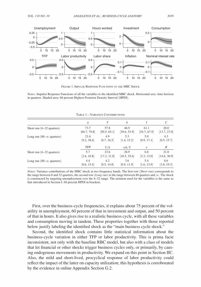
Figure 1 reports the impulse response functions (IRFs) of all the variables to this shock. As very similar IRFs are produced by the shocks that target the other key macroeconomic quantities, this figure plays a crucial role in our analysis: it serves as the empirical template for the propagation mechanism of models that contain a single or dominant business-cycle driver.
Table 1 adds more information about the identified shock by reporting its contri-bution to the volatility of all the variables over two frequency bands: the one used to construct it, which corresponds to the range between 6 and 32 quarters and is referred to as Short run in the table; and a different band, which is referred to as Long run and corresponds to the range between 80 quarters and ∞ . This helps assess whether the identified shock can indeed account for the bulk of the business-cycle fluctuations in the key macroeconomic quantities, as well as how large its footprint is on inflation or the long run.11
What are the main properties of the identified shock?
10 Our method also brings principle component analysis (PCA) to mind. We explore this relation in Section IIIA.11 Online Appendix Figure 12 contains similar information in terms of the contributions of the identified shock
to forecast error variances (FEV) at different horizons.
3039ANGELETOS ET AL.: BUSINESS-CYCLE ANATOMYVOL. 110 NO. 10
First, over the business-cycle frequencies, it explains about 75 percent of the vol-atility in unemployment, 60 percent of that in investment and output, and 50 percent of that in hours. It also gives rise to a realistic business cycle, with all these variables and consumption moving in tandem. These properties together with those reported below justify labeling the identified shock as the “main business cycle shock.”
Second, the identified shock contains little statistical information about the business-cycle variation in either TFP or labor productivity. This is prima facie inconsistent, not only with the baseline RBC model, but also with a class of models that let financial or other shocks trigger business cycles only, or primarily, by caus-ing endogenous movements in productivity. We expand on this point in Section IIC. Also, the mild and short-lived, procyclical response of labor productivity could reflect the impact of the latter on capacity utilization; this hypothesis is corroborated by the evidence in online Appendix Section G.2.
Table 1—Variance Contributions
u Y h I C
Short run (6–32 quarters) 73.7 57.8 46.9 61.1 20.0[66.7, 79.8] [50.5, 65.1] [39.6, 53.9] [54.7, 67.9] [13.7, 27.0]
Long run (80– ∞ quarters) 21.6 4.9 5.3 5.0 4.3[9.2, 38.6] [0.7, 16.5] [1.4, 15.2] [0.9, 17.1] [0.5, 15.7]
TFP Y / h wh / Y π R
Short run (6–32 quarters) 5.7 23.6 26.9 6.8 21.8[2.6, 10.8] [17.2, 31.0] [18.5, 35.6] [3.3, 12.0] [14.6, 30.9]
Long run (80– ∞ quarters) 4.4 4.2 3.6 5.4 8.6[0.6, 15.4] [0.5, 14.8] [0.9, 11.9] [1.6, 13.9] [3.0, 19.3]
Notes: Variance contributions of the MBC shock at two frequency bands. The first row (Short run) corresponds to the range between 6 and 32 quarters, the second row (Long run) to the range between 80 quarters and ∞ . The shock is constructed by targeting unemployment over the 6 – 32 range. The notation used for the variables is the same as that introduced in Section I. 68 percent HPDI in brackets.
Figure 1. Impulse Response Functions to the MBC Shock
Notes: Impulse Response Functions of all the variables to the identified MBC shock. Horizontal axis: time horizon in quarters. Shaded area: 68 percent Highest Posterior Density Interval (HPDI).
5 10 15 20 5 10 15 20 5 10 15 20 5 10 15 20 5 10 15 20
5 10 15 20
0.25 1
−0.25
−0.5
−0.5
0.5
0
−0.5
0.5
0
−0.5
0.5
0
−0.1
0.1
0
−0.1
0.1
0
0
0
0
0.5
1
0
0.5
0.52
0
5 10 15 20 5 10 15 20 5 10 15 20 5 10 15 20
Unemployment Output Hours worked Investment Consumption
TFP Labor productivity Labor share In�ation Nominal interest rate

3040 THE AMERICAN ECONOMIC REVIEW OCTOBER 2020
Third, the effect on macroeconomic activity peaks within a year of its occurrence, fades out before long, and leaves a negligible footprint on the long run. This finding extends and reinforces the message of Blanchard and Quah (1989): what drives the business cycle appears to be distinct from what drives productivity and output in the longer term. This point is further corroborated later.
Fourth, the shock triggers a small, almost negligible, and delayed movement in inflation. This precludes the interpretation of the identified shock as an inflationary demand shock of the textbook variety. But it leaves two other interpretations open: a demand shock of the DSGE variety (a shock that moves output but not inflation due to a very flat Phillips curve); or a demand shock that operates outside the realm of nominal rigidities as in the models cited in footnote 3. We revisit this point in Sections IID and V.
Fifth, the shock triggers a strong, procyclical movement in the nominal interest rate, and in the real interest rate, too, since inflation hardly moves. At face value, this seems consistent with a monetary policy that raises the nominal interest in response to the boom triggered by the identified shock, stabilizes inflation, and per-haps even closes the gap from flexible-price outcomes (or, equivalently, tracks the natural rate of interest). This scenario is ruled out in the prevailing New Keynesian paradigm, because a gap from flexible-price outcomes is needed in order to accom-modate demand-driven business cycles. But there is no way to verify or reject this assumption on purely empirical grounds, because the natural rate of interest and the flexible-price outcomes are not directly observable (and not even defined outside specific models).
Finally, the shock triggers a countercyclical response in the labor share for the first few quarters, which is reversed later on. Relatedly, when looking at the response of the real wage, as inferred by the difference between the response of the labor share and that of labor productivity, we see that the real wage remains relatively flat in response to the identified shock. This is consistent with the well-known, uncon-ditional fact that real wages display very weak procyclicality, which is typically interpreted as being due to some form of real-wage rigidity.
B. The Main Business-Cycle Shock: Targeting Other Quantities
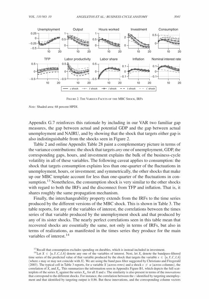
Figure 2 compares the IRFs of the shock that targets the business-cycle volatility of the unemployment rate (black line) to the IRFs of the shocks that are identified by targeting the business-cycle volatility of some other key macroeconomic quantities: GDP, hours, investment, and consumption.
As is evident from the figure, these shocks are nearly indistinguishable: tar-geting any one of the aforementioned variables seems to give rise to the same dynamic comovement properties. This explains the rationale of interpreting these reduced-form shocks as interchangeable facets of the empirical footprint of the same propagation mechanism, or of what we have called the MBC shock.12 Online
12 Recall that, for our purposes, different shocks that are observationally equivalent in terms of IRFs are essen-tially one and the same shock. This perspective is consistent with standard practice in both the SVAR and the DSGE literatures: as echoed in the quote from Cochrane cited in footnote 2, shocks are visible, and hence distinguishable, only through the dynamic comovement patterns they induce in the variables of interest.
3041ANGELETOS ET AL.: BUSINESS-CYCLE ANATOMYVOL. 110 NO. 10
Appendix G.7 reinforces this rationale by including in our VAR two familiar gap measures, the gap between actual and potential GDP and the gap between actual unemployment and NAIRU, and by showing that the shock that targets either gap is also indistinguishable from the shocks seen in Figure 2.
Table 2 and online Appendix Table 28 paint a complementary picture in terms of the variance contributions: the shock that targets any one of unemployment, GDP, the corresponding gaps, hours, and investment explains the bulk of the business-cycle volatility in all of these variables. The following caveat applies to consumption: the shock that targets consumption explains less than one-quarter of the fluctuations in unemployment, hours, or investment; and symmetrically, the other shocks that make up our MBC template account for less than one-quarter of the fluctuations in con-sumption.13 Nonetheless, the consumption shock is very similar to the other shocks with regard to both the IRFs and the disconnect from TFP and inflation. That is, it shares roughly the same propagation mechanism.
Finally, the interchangeability property extends from the IRFs to the time series produced by the different versions of the MBC shock. This is shown in Table 3. The table reports, for any of the variables of interest, the correlations between the times series of that variable produced by the unemployment shock and that produced by any of its sister shocks. The nearly perfect correlations seen in this table mean that recovered shocks are essentially the same, not only in terms of IRFs, but also in terms of realizations, as manifested in the times series they produce for the main variables of interest.14
13 Recall that consumption excludes spending on durables, which is instead included in investment.14 Let X ∈ {u, Y, C, I, h} denote any one of the variables of interest. Next, let X s denote the bandpass-filtered
time series of the predicted value of that variable produced by the shock that targets the variable s ∈ {u, Y, C, I, h} (where s may or may not coincide with X ). We are using the band pass filter suggested by Christiano and Fitzgerald (2003). The typical cell in Table 3 reports, for a variable X (across rows) and a shock s ≠ u (across columns), the correlation of X s and X u . This summarizes the information seen in Appendix Figure B1, which depicts the full scat-terplots of the series X s against the series X u , for all X and s . The similarity is also present in terms of the innovations that correspond to the different shocks. For instance, the correlation between the ε identified by targeting unemploy-ment and that identified by targeting output is 0.86. But these innovations, and the corresponding column vectors
Figure 2. The Various Facets of the MBC Shock, IRFs
Note: Shaded area: 68 percent HPDI.
10 20
Unemployment
10 20
Output
10 20
Hours worked
10 20
Investment
10 20
10 20
0.25
0.5
−0.5
−0.25
−0.5
0
0
0.5
−0.5
0
0.5
−0.5
0
0.1
−0.1
0
0.1
−0.1
0
0
0.5
1
0 00
20.5
0.51
10 20 10 20 10 20 10 20
Consumption
TFP Labor productivity Labor share In�ation Nominal interest rate
u shock Y shock I shock h shock C shock

3042 THE AMERICAN ECONOMIC REVIEW OCTOBER 2020
C. The Long Run and the Short Run
In the preceding analysis we recovered a MBC shock by targeting the business cycle frequencies. We now document the existence of an analogous object for the long-run frequencies. We also discuss the implications of our results for theories that link the business cycle to technology and news shocks.
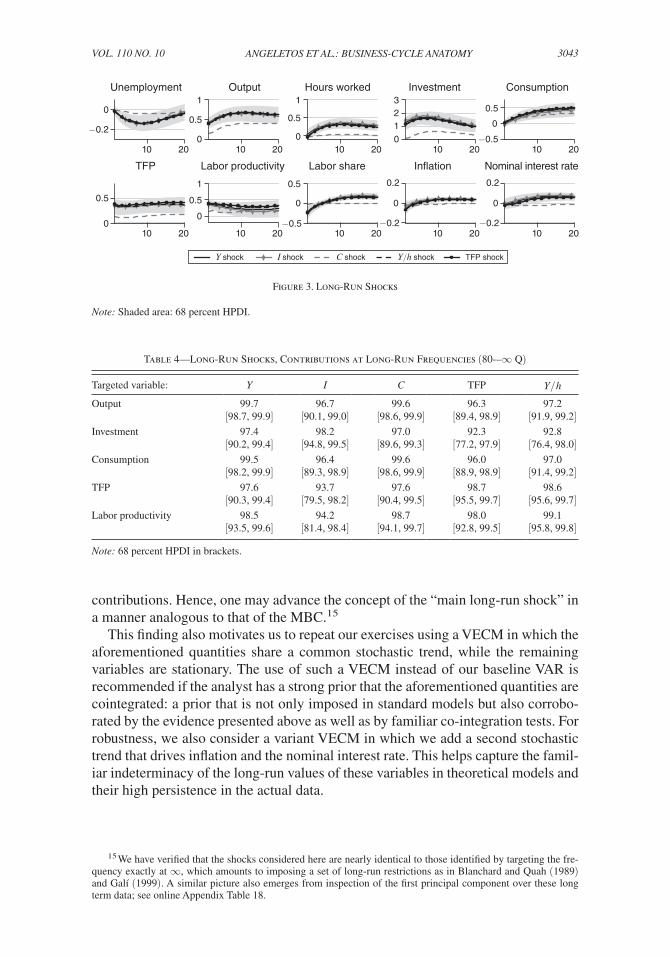
Consider the shocks that target GDP, investment, consumption, TFP, and labor productivity at the frequencies corresponding to 80– ∞ quarters. Figure 3 and Table 4 show that these shocks are nearly indistinguishable in terms of IRFs and variance
of the matrix Q , are not sufficiently meaningful in their own right. What matters is how these innovations propagate over time and across variables, which is what the IRFs seen in Figure 2 reveal, or how they manifest themselves in terms of the predicted time series X s , which explains the focus of Table 3 and Figure 9.
Table 2—The Various Facets of the MBC Shock, Variance Contributions
Targeted variable: u Y h I C
Unemployment 73.7 57.8 46.9 61.1 20.0[66.7, 79.8] [50.5, 65.1] [39.6, 53.9] [54.7, 67.9] [13.7,27.0]
Output 55.6 79.8 44.0 66.5 32.6[49.6, 61.7] [72.9, 86.2] [36.7,51.3] [61.0, 72.6] [26.0,39.2]
Hours worked 49.0 46.5 70.0 46.7 21.7[41.8, 56.3] [38.0, 55.3] [63.0, 76.7] [37.3, 55.6] [15.6,28.5]
Investment 58.2 66.2 44.4 80.1 18.8[52.3, 64.0] [60.2, 72.3] [36.8, 51.9] [73.5, 86.6] [12.5,26.3]
Consumption 18.3 30.9 19.5 16.2 67.8[12.2, 25.8] [22.5, 39.3] [13.4, 26.1] [10.2, 24.1] [60.7, 75.3]
Targeted variable: TFP Y / h wh / Y π R
Unemployment 5.7 23.6 26.9 6.8 21.8[2.6, 10.8] [17.2, 31.0] [18.5, 35.6] [3.3, 12.0] [14.6, 30.9]
Output 4.1 41.0 40.5 10.6 16.8[1.7, 8.4] [35.3, 47.2] [33.7, 46.8] [6.1, 16.1] [10.3, 25.0]
Hours worked 11.5 22.0 19.4 7.0 22.4[6.4, 18.2] [15.4, 29.4] [11.1, 29.5] [3.5, 12.5] [14.6, 31.5]
Investment 3.7 33.9 36.5 7.4 20.6[1.3, 7.9] [27.7, 40.2] [29.5, 43.4] [3.6, 12.5] [13.3, 29.1]
Consumption 1.5 12.6 9.8 9.5 4.5[0.6, 3.4] [7.4, 18.4] [5.0, 16.9] [4.6, 16.9] [1.3, 10.3]
Notes: The rows correspond to different targets in the construction of the shock. The columns give the contributions of the constructed shock to the business-cycle volatility of the variables. 68 percent HPDI in brackets.
Table 3—Correlations of Conditional Times Series
Y shock I shock C shock h shock
Unemployment 0.971 0.981 0.923 0.939Output 0.997 0.997 0.989 0.992Investment 0.990 0.996 0.934 0.989Consumption 0.986 0.982 0.744 0.961Hours worked 0.971 0.981 0.923 0.939
Note: Each row reports the correlation between each bandpass-filtered variable as predicted by the unemployment shock and that predicted by the other facets of the MBC shock.
3043ANGELETOS ET AL.: BUSINESS-CYCLE ANATOMYVOL. 110 NO. 10
contributions. Hence, one may advance the concept of the “main long-run shock” in a manner analogous to that of the MBC.15
This finding also motivates us to repeat our exercises using a VECM in which the aforementioned quantities share a common stochastic trend, while the remaining variables are stationary. The use of such a VECM instead of our baseline VAR is recommended if the analyst has a strong prior that the aforementioned quantities are cointegrated: a prior that is not only imposed in standard models but also corrobo-rated by the evidence presented above as well as by familiar co-integration tests. For robustness, we also consider a variant VECM in which we add a second stochastic trend that drives inflation and the nominal interest rate. This helps capture the famil-iar indeterminacy of the long-run values of these variables in theoretical models and their high persistence in the actual data.
15 We have verified that the shocks considered here are nearly identical to those identified by targeting the fre-quency exactly at ∞ , which amounts to imposing a set of long-run restrictions as in Blanchard and Quah (1989) and Galí (1999). A similar picture also emerges from inspection of the first principal component over these long term data; see online Appendix Table 18.
Figure 3. Long-Run Shocks
Note: Shaded area: 68 percent HPDI.
10
0
0
0
0.5
0.5
1
0
0.5
−0.5
1
00
0.5
−0.5
0
0.2
−0.2
0
0.2
−0.2
00.5
1
3210
−0.2
20
Unemployment
10 20
Output
10 20
Hours worked
10 20
Investment
10 20
10 20 10 20 10 20 10 20 10 20
Consumption
TFP Labor productivity Labor share In�ation Nominal interest rate
Y shock I shock C shock Y/h shock TFP shock
0.5
Table 4—Long-Run Shocks, Contributions at Long-Run Frequencies (80-– ∞ Q)
Targeted variable: Y I C TFP Y / h
Output 99.7 96.7 99.6 96.3 97.2[98.7, 99.9] [90.1, 99.0] [98.6, 99.9] [89.4, 98.9] [91.9, 99.2]
Investment 97.4 98.2 97.0 92.3 92.8[90.2, 99.4] [94.8, 99.5] [89.6, 99.3] [77.2, 97.9] [76.4, 98.0]
Consumption 99.5 96.4 99.6 96.0 97.0[98.2, 99.9] [89.3, 98.9] [98.6, 99.9] [88.9, 98.9] [91.4, 99.2]
TFP 97.6 93.7 97.6 98.7 98.6[90.3, 99.4] [79.5, 98.2] [90.4, 99.5] [95.5, 99.7] [95.6, 99.7]
Labor productivity 98.5 94.2 98.7 98.0 99.1[93.5, 99.6] [81.4, 98.4] [94.1, 99.7] [92.8, 99.5] [95.8, 99.8]
Note: 68 percent HPDI in brackets.

3044 THE AMERICAN ECONOMIC REVIEW OCTOBER 2020
These VECMs produce the same empirical properties for the MBC shock as those derived from the VARs and presented above. They also produce similar pat-terns regarding the properties of the long-run shock. Table 5 demonstrates this with regard to the business cycle footprint of the long-run shock. This table reports the contribution of the main long-run shock, represented by the shock that targets TFP over the 80– ∞ range, to the volatilities of all the variables over the 6–32 range. The emerging picture is essentially the mirror image of that contained in the second row of Table 1. There, we reported that the MBC shock has a small contribution to the long run. Here, we see that the shock that accounts for the long run has a small footprint on the business cycle.
The disconnect between the short and the long run can also be seen in Figure 4, which shows the contribution of the MBC shock to the forecast error variance (FEV) of unemployment, output, and TFP at different time horizons.16 The MBC shock explains more than 60 percent of unemployment and output movements during the first two years, but less than 7 percent of the TFP movements at any horizon; and conversely, the main long-run shock explains nearly all the long-run variation in investment and TFP, but less than 10 percent of the unemployment and investment movements over the first two years.17
How do these findings compare to related ones in the existing literature?First, consider Blanchard and Quah (1989). This paper seeks to represent the data
in terms of two shocks, a “supply shock” and a “demand shock.” To this goal, they run a VAR on two variables, GDP and unemployment; identify the supply shock as the shock that accounts for GDP movements in the very long run (at ∞ ) and the demand shock as the residual shock; and document that the supply shock accounts for about 50 percent of the business-cycle volatility in GDP and a bit more of that in unemployment. The additional information contained in our larger VAR reduces the contribution of the supply shock to about 12 percent for GDP and for unemployment.
16 The MBC shock is still identified in the frequency domain. The same picture emerges when the MBC is identified in the time domain, provided that one uses the “right” mapping between the two domains. See online Appendix Section E.
17 It is worth noting that the disconnect between the short and the long run extends from neutral technology, as measured by TFP, to investment-specific technology, as measured by the relative price of investment; see online Appendix Section G.2.
Table 5—Long-Run TFP Shock, Contributions at Business-Cycle Frequencies
u Y h I C
VAR 9.7 25.7 11.5 18.6 15.7[3.9, 18.9] [11.7, 42.5] [5.1, 20.1] [8.2, 31.3] [6.7, 27.9]
VECM 12.1 11.7 8.0 10.6 8.6[4.8, 22.1] [4.7, 22.4] [2.8, 16.3] [4.5, 19.3] [2.3, 18.5]
TFP Y / h wh / Y π R
VAR 21.4 22.9 10.2 13.1 8.1[6.6, 41.8] [11.4, 36.4] [2.8, 23.2] [4.9, 27.8] [2.8, 16.9]
VECM 11.5 11.2 9.5 7.7 11.1[3.8, 26.6] [5.0, 22.4] [4.2, 18.6] [2.4, 21.1] [3.5, 25.2]
Note: 68 percent HPDI in brackets.

3045ANGELETOS ET AL.: BUSINESS-CYCLE ANATOMYVOL. 110 NO. 10
Second, consider Uhlig (2003), which is the closest predecessor to our paper. Similarly to Blanchard and Quah (1989), Uhlig (2003) pursues a two-shock rep-resentation of the data. The two shocks are identified by jointly maximizing the forecast error variance (FEV) in real GNP for horizons between 0 and 5 years. Uhlig offers a tentative interpretation of one shock as being a productivity shock of the RBC type and the other as a cost-push shock of the New Keynesian type. This interpretation finds little support in our more extensive anatomy of the data, especially due to our finding of a disconnect between our MBC shock and TFP at all horizons.18 Furthermore, as explained in Section IIIB, once we move from the frequency to the time domain, the business cycle is best captured by targeting the FEVs of unemployment and GDP at 1 year, as opposed to longer horizons.
Third, consider Galí (1999) and Neville et al. (2014). Our long-run TFP shock is essentially the same as the technology shock identified in those papers. Tables 4 and 5 confirm their finding that this shock has a small contribution to the business cycle. This extends to the robustness exercises reviewed in Section IIIC.
Finally, consider Beaudry and Portier (2006). The first part of that paper uses a two-variable VAR with TFP and the S&P500 index to identify a shock that has zero impact effect on TFP but accounts for the bulk of both the short-run movements in stock prices and the long-run movements in TFP. This shock is interpreted as “news” about future TFP. The second part proceeds to argue, using 3–5-variable VARs and additional identifying restrictions, that TFP news shocks account for about 50 per-cent of the short-run volatility in hours and total private spending, about 80 percent of that in consumption, and about 80 percent the long-run movements in private spending. In short, TFP news emerges as the main driver of both the business cycle and the long run.
This picture is hard to reconcile with our results, as well as with those of Galí (1999) and Neville et al. (2014). If TFP news was the main driver of both the busi-ness cycle and the long run, one would expect to see a strong connection between the two. But as seen in Table 5, the main long-run shock identified here accounts for only 10 percent of the short-run volatility in unemployment, hours, and investment. A similar disconnect is found in Galí (1999) and Neville et al. (2014).
18 We emphasize that the interpretation offered in Uhlig (2003) was tentative as that paper was not completed. Also note that the approach adopted in that paper allows for the identification of the two shocks together but does not separate one shock from the other, so the aforementioned interpretation relied on particular orthogonalizations. Finally, because the VAR considered in that paper did not contain TFP, the disconnect documented here could not have been detected.
Figure 4. FEVs of Unemployment, GDP, and TFP to the MBC Shock
Note: Shaded area: 68 percent HPDI.
20 40 60 80Quarters
Per
cent
Panel A. Unemployment
20 40 60 80Quarters
Per
cent
Panel B. Output
20 40 60 80Quarters
0
20
40
60
80
100
Per
cent
Panel C. TFP
0
20
40
60
80
100
0
20
40
60
80
100

3046 THE AMERICAN ECONOMIC REVIEW OCTOBER 2020
Perhaps most tellingly, Figure 4 shows that the MBC shock accounts for nearly zero of the FEV of TFP at any horizon. That is, the MBC shock itself contains no news about future TFP.19
We believe that, while TFP news may be a nontrivial contributor to macroeco-nomic fluctuations, the numbers reported by Beaudry and Portier (2006) exaggerate its importance due to the use of smaller VARs and different identifying assumptions. We elaborate on these points in Section IV and Appendix Section C. There, we use a semistructural exercise, based on our anatomy of the data, to shed new light on the business-cycle effects of technology and news shocks. Our explorations suggest that the contribution of news shocks to unemployment fluctuations is about 10 percent, which is much more modest than that suggested by Beaudry and Portier (2006) and closer to that reported in Barsky and Sims (2011).
A similar challenge applies to Lorenzoni (2009). That paper emphasizes the role of noise in the signals of future TFP, but maintains the core hypothesis that the busi-ness cycle is driven by shifts in the rational expectations of the long run, which is hard to reconcile with our findings.20
What is left open is the possibility that the identified MBC shock reflects either irrational beliefs about the long run, or news about the short run. A formalization of the latter kind of news is found in our companion paper (Angeletos, Collard, and Dellas 2018), to which we return in Section V.
D. Inflation and the Business Cycle
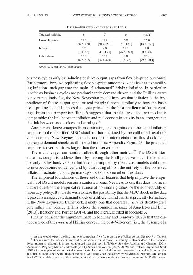
We now turn attention to the nexus of real economic activity and inflation. Our method identifies a weak link. First, as shown in the first row of Table 6 (which repeats a portion of the first row of Table 1), the identified MBC shock accounts for only 7 percent of the business-cycle variation in inflation, which is as low as the corre-sponding number for TFP. Second, the shock that targets inflation explains 83 percent of the business-cycle volatility in inflation and only 4 to 8 percent of that in unem-ployment, output, and investment. Third, the shock that targets inflation explains only 2 percent of the labor share, a proxy of the real marginal cost or the “fundamental” in the New Keynesian Phillips Curve (Galí and Gertler 1999); and symmetrically, the shock that targets the labor share explains 86 percent of the labor share itself but only 4 percent of inflation. Fourth, the shock that targets inflation is essentially orthogonal to the MBC shock, both in terms of innovations and in terms of induced series. For instance, the correlation between the ε identified by targeting inflation and that iden-tified by targeting unemployment is 0.047. Finally, online Appendix Sections G.6 and G.7 show that these findings are robust to different measures of inflation (GDP deflator versus CPI, PPI, or core inflation) and different measures of real slackness (unemployment versus unemployment gap or output gap).
What is the lesson for theory? Because of its transitory nature and its disconnect from TFP, it is tempting to interpret the MBC shock in the data as a demand shock in the New Keynesian model. However, in that model demand shocks generate
19 As verified in row 9 of Table 8, these findings are robust to the inclusion of Stock Prices in the VAR.20 By shifting the focus from the distinct theoretical formulation of news and noise shocks to their shared empir-
ical footprint in terms of VAR representations, we echo Chahrour and Jurado (2018).
3047ANGELETOS ET AL.: BUSINESS-CYCLE ANATOMYVOL. 110 NO. 10
business cycles only by inducing positive output gaps from flexible-price outcomes. Furthermore, because replicating flexible-price outcomes is equivalent to stabiliz-ing inflation, such gaps are the main “fundamental” driving inflation. In particular, insofar as business cycles are predominantly demand-driven and the Phillips curve is not exceedingly flat, the New Keynesian model imposes that inflation is the best predictor of future output gaps, or real marginal costs, similarly to how the basic asset-pricing model imposes that asset prices are the best predictor of future earn-ings. From this perspective, Table 6 suggests that the failure of the two models is comparable: the link between inflation and real economic activity is no stronger than the link between asset prices and earnings.21
Another challenge emerges from contrasting the magnitude of the actual inflation response to the identified MBC shock to that predicted by the calibrated, textbook version of the New Keynesian model under the interpretation of this shock as an aggregate demand shock: as illustrated in online Appendix Figure 25, the predicted response is over ten times larger than the observed one.
These challenges are familiar, albeit through other metrics.22 The DSGE liter-ature has sought to address them by making the Phillips curve much flatter than, not only its textbook version, but also that implied by menu-cost models calibrated to microeconomic evidence; and by attributing almost the entirety of the observed inflation fluctuations to large markup shocks or some other “residual.”
The empirical foundations of these and other features that help improve the empir-ical fit of DSGE models remain a contested issue. Needless to say, this does not mean that we question the empirical relevance of nominal rigidities, or the nonneutrality of monetary policy. But we do wish to raise the possibility that the MBC shock in the data represents an aggregate demand shock of a different kind than that presently formalized in the New Keynesian framework, namely one that operates inside its flexible-price core rather than outside it. This echoes the common message of Angeletos and La’O (2013), Beaudry and Portier (2014), and the literature cited in footnote 3.
Finally, consider the argument made in McLeay and Tenreyro (2020) that the dis-appearance of the empirical Phillips curve in the post-Volker era (i.e., the absence of a
21 As one would expect, the link improves somewhat if we focus on the pre-Volker period. See row 7 of Table 8.22 For instance, the weak comovement of inflation and real economic activity is also evident in the uncondi-
tional moments, although it is less pronounced than that seen in Table 6. See also Atkeson and Ohanian (2001); Mavroeidis, Plagborg-Møller, and Stock (2014); Stock and Watson (2007, 2009); and Dotsey, Fujita, and Stark (2018) for examples of works that document a similar statistical disconnect between gaps and inflation as that documented here, albeit with different methods. And finally see the survey by Mavroeidis, Plagborg-Møller, and Stock (2014) and the references therein for empirical performance of the various incarnations of the Phillips curve.
Table 6—Inflation and the Business Cycle
Targeted variable: u Y π wh/Y
Unemployment 73.7 57.8 6.8 26.9[66.7, 79.8] [50.5, 65.1] [3.3, 12.0] [18.5, 35.6]
Inflation 4.2 8.0 83.3 1.9[1.8, 8.6] [4.0, 13.1] [76.2, 88.3] [0.7, 4.4]
Labor share 26.0 35.6 4.0 85.4[18.7, 33.5] [28.8, 42.6] [1.7, 7.6] [79.8, 90.4]
Note: 68 percent HPDI in brackets.

3048 THE AMERICAN ECONOMIC REVIEW OCTOBER 2020
strong positive relation between inflation and the output gap) may reflect a monetary policy that has done a good job in stabilizing the output gap against demand shocks and has let inflation be driven primarily by “residual” shocks. This argument may explain the disconnect seen in Table 6 in terms of variance contributions. But another key piece of evidence produced by our anatomy is the muted response of inflation to the MBC shock (seen earlier in Figures 1 and 2). This in turn requires either that the structural Phillips curve is exceedingly flat,23 which runs against the thesis of the aforementioned paper, or that the MBC shock is a demand shock that generates real-istic business cycles even when monetary policy replicates flexible-price allocations, which circles back to our preferred interpretation of the evidence.
III. Robustness
In this section we first discuss the relation between our approach and two alterna-tives: principal component analysis, and identification in the time domain. We next report results from an extensive battery of robustness exercises conducted.
A. The MBC Shock and Principal Component Analysis
The finding that there is a single force that drives multiple measures of economic activity naturally invites a comparison to principal component analysis (PCA). Is our MBC shock similar to the first principal component of the data over business-cy-cle frequencies? And if yes, are there any reasons to favor employing our method over PCA in pursuing an anatomy of the business cycle?24
To address the first question, we perform PCA in the frequency domain. For each variable X j ∈ {u, Y, h, I, …} , we construct the bandpass-filtered variable X j bc that isolates its business cycle frequencies ( 6–32 quarters). We then use the cova-riance matrix of all the filtered variables to construct the first principal component, denoted by PC 1 bc . We finally project each X j bc on PC 1 bc and compute the R2 of the projection. This gives the percentage of the business-cycle volatility in variable j accounted for by the principal component.25
Four different versions of this exercise are carried out. In the first version, X bc is derived by applying the bandpass filter directly on the raw data, variable by vari-able. In the second version, we first run a VAR on all the variables jointly, use it to estimate the cross-spectrum of the data, and then construct the band passed vari-ables X j bc . Hence, the bandpass filter is the ideal one in the latter case, whereas it is only an approximate one in the former.
In the third and fourth version, the filtered variables are normalized by their respective standard deviations before extracting the first principal component. Such a normalization is often employed in the PCA literature in order to cope with scaling
23 See online Appendix Section I.1 for the illustration of this point when the MBC shock maps directly to a demand shock in the New Keynesian model; and see online Appendix Section I.2 for the robustness of this point to letting the MBC shock map to a mixture of demand and supply shocks in the model.
24 We thank an anonymous referee for suggesting the exploration of these questions.25 Recall that the first principal component is constructed by taking the eigenvector corresponding to the largest
eigenvalue of the covariance matrix. It is thus designed to account for as much as possible of the volatility and the comovement of all the (filtered) variables at once.
3049ANGELETOS ET AL.: BUSINESS-CYCLE ANATOMYVOL. 110 NO. 10
issues and/or to focus on the comovements in the data. But it also reduces the role played by the more volatile variables (e.g., investment), which may or may not be desirable depending on the context. As we do not have a strong prior on how to properly weight the variables, we carry the exercise on both normalized and nonnormalized data.
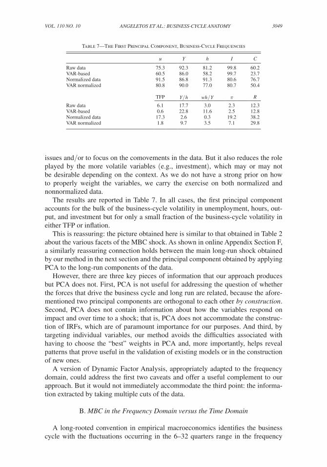
The results are reported in Table 7. In all cases, the first principal component accounts for the bulk of the business-cycle volatility in unemployment, hours, out-put, and investment but for only a small fraction of the business-cycle volatility in either TFP or inflation.
This is reassuring: the picture obtained here is similar to that obtained in Table 2 about the various facets of the MBC shock. As shown in online Appendix Section F, a similarly reassuring connection holds between the main long-run shock obtained by our method in the next section and the principal component obtained by applying PCA to the long-run components of the data.
However, there are three key pieces of information that our approach produces but PCA does not. First, PCA is not useful for addressing the question of whether the forces that drive the business cycle and long run are related, because the afore-mentioned two principal components are orthogonal to each other by construction. Second, PCA does not contain information about how the variables respond on impact and over time to a shock; that is, PCA does not accommodate the construc-tion of IRFs, which are of paramount importance for our purposes. And third, by targeting individual variables, our method avoids the difficulties associated with having to choose the “best” weights in PCA and, more importantly, helps reveal patterns that prove useful in the validation of existing models or in the construction of new ones.
A version of Dynamic Factor Analysis, appropriately adapted to the frequency domain, could address the first two caveats and offer a useful complement to our approach. But it would not immediately accommodate the third point: the informa-tion extracted by taking multiple cuts of the data.
B. MBC in the Frequency Domain versus the Time Domain
A long-rooted convention in empirical macroeconomics identifies the business cycle with the fluctuations occurring in the 6–32 quarters range in the frequency
Table 7—The First Principal Component, Business-Cycle Frequencies
u Y h I C
Raw data 75.3 92.3 81.2 99.8 60.2VAR-based 60.5 86.0 58.2 99.7 23.7Normalized data 91.5 86.8 91.3 80.6 76.7VAR normalized 80.8 90.0 77.0 80.7 50.4
TFP Y / h wh / Y π R
Raw data 6.1 17.7 3.0 2.3 12.3VAR-based 0.6 22.8 11.6 2.5 12.8Normalized data 17.3 2.6 0.3 19.2 38.2VAR normalized 1.8 9.7 3.5 7.1 29.8

3050 THE AMERICAN ECONOMIC REVIEW OCTOBER 2020
domain (FD).26 In line with this tradition, our MBC shock is constructed by identi-fying the shock that accounts the most of the volatility of unemployment and other key macro quantities in that range.
But suppose one wished to identify business cycles in the time domain (TD) instead. Which horizon(s) should one target?
At first glance, one may think that targeting volatility over the 6–32 quarters band in the FD is equivalent to targeting volatility over the 6–32 quarters horizon range in the TD. But this is wrong: such a relation does not hold for arbitrary DGPs (or arbitrary models), nor does it hold in the actual data.
We offer a comprehensive treatment of this issue in Appendix Section E by under-taking two exercises, one theoretical and one empirical.
In the first exercise, we set up a 3 × 3 model (three variables, three shocks). Although the model is deliberately abstract, its variables can loosely be interpreted as unemployment, output, and inflation. Its main purpose is to serve as a controlled laboratory environment, in which we can work out the properties of alternative map-pings between the FD and the TD.
Within this controlled environment, we establish two properties of the MBC shock identified via our method, that is, by targeting the volatility of the first two variables over the 6–32 quarters in the FD: (i) this shock is notably different from the shock that targets 6–32 quarters in the TD; and (ii) this shock is nearly identical to the one that targets 4 quarters in the TD. This serves both as a proof of concept that the mapping between the FD and the TD is nontrivial in general, and as an illus-tration of the kind of model that best fits the data.
The second exercise completes the picture by showing that the two properties mentioned above indeed characterize the data. A hint that the second property is true in the data was already present in Figures 1 and 4, which showed that the footprint of our MBC shock in the TD, in terms of both IRFs and FEVs, peaked within a year or so.
These findings complement the picture painted in the rest of our paper. They also illustrate why TD-based identification strategies that maximize the FEV contribu-tion of a shock to unemployment or output at longer horizons could fail to capture business cycles.
C. Alternative Specifications
We now turn to the robustness of our main results along various dimensions (sample periods, set of variables, assumptions about stationarity, numbers of lags). The main exercises are described below; a few additional ones are relegated to the online Appendix.
Table 8 describes the variance contribution of the MBC shock over business-cy-cle and longer-term frequencies, respectively, and across many alternative specifi-cations (different samples, statistical models estimated, set of variables, numbers of lags). As in Table 1, we use the shock that targets unemployment as the measure of
26 This convention stretches back at least to Mitchell. More recently, when researchers document business-cycle moments whether in the data or in a model, they almost invariably use either the BP filter at the 6–32 quarters band or the HP filter, which is closely related (e.g., Stock and Watson 1999).

3051ANGELETOS ET AL.: BUSINESS-CYCLE ANATOMYVOL. 110 NO. 10
Table 8—Robustness, Variance Contributions
Short-run contribution
u Y h I C
1. Benchmark 73.7 57.8 46.9 61.1 20.0[66.7, 79.8] [50.5, 65.1] [39.6, 53.9] [54.7, 67.9] [13.7, 27.0]
2. 4 lags 74.4 57.7 48.8 62.0 20.8[67.1, 80.6] [49.7, 64.8] [41.7, 55.8] [54.7, 69.0] [13.9, 28.3]
3. VECM(1) 62.5 52.4 48.2 54.6 36.6[56.4, 68.9] [44.6, 59.3] [40.9, 54.8] [47.8, 60.7] [26.9, 47.1]
4. VECM(2) 65.1 54.7 49.8 54.4 43.7[58.7, 72.0] [47.7, 62.3] [43.5, 56.2] [48.3, 61.8] [32.1, 54.5]
5. 1948–2017 78.2 64.8 49.2 63.5 19.9[72.4, 84.1] [58.6, 70.9] [43.4, 55.9] [57.0, 69.7] [13.7, 26.7]
6. 1960–2007 69.1 60.4 49.8 62.7 24.5[61.9, 75.4] [51.6, 67.5] [42.4, 56.7] [54.8, 69.8] [16.6, 34.9]
7. pre-Volcker 73.6 56.1 42.6 60.7 22.1[63.6, 82.3] [46.1, 64.8] [32.2, 52.5] [51.6, 69.2] [12.6, 33.5]
8. post-Volcker 73.4 50.4 50.4 58.3 20.0[64.8, 79.7] [41.8, 58.2] [41.7, 58.8] [50.1, 65.7] [12.3, 29.0]
9. Extended 59.5 50.5 45.8 53.2 22.1[53.8, 65.5] [43.1, 58.2] [39.4, 51.3] [44.7, 59.7] [15.1, 31.3]
10. Financial 68.5 57.9 46.6 59.9 26.0[62.1, 75.1] [50.0, 64.3] [39.5, 54.1] [52.6, 66.7] [17.9, 34.6]
11. Chained C&I 81.7 58.5 46.1 61.1 17.1[75.8, 86.7] [52.1, 64.5] [39.3, 52.1] [55.1, 67.1] [11.7, 23.4]
Short-run contribution Long-run contribution
π TFP Y TFP
1. Benchmark 6.8 5.7 4.9 4.4[3.3, 12.0] [2.6, 10.8] [0.7, 16.5] [0.6, 15.4]
2. 4 lags 6.7 6.3 4.2 3.6[3.1, 12.1] [2.7, 11.3] [0.6, 14.1] [0.5, 13.0]
3. VECM(1) 8.8 13.1 13.7 13.7[3.9, 18.1] [6.3, 23.4] [3.0, 32.0] [3.0, 32.0]
4. VECM(2) 12.2 14.4 15.8 15.8[6.1, 20.4] [7.3, 23.2] [3.7, 33.5] [3.7, 33.5]
5. 1948–2017 5.7 6.2 6.6 6.1[2.3, 10.2] [2.5, 11.2] [1.0, 18.4] [0.9, 18.4]
6. 1960–2007 12.4 5.3 3.3 3.2[6.1, 20.3] [2.2, 11.3] [0.5, 12.6] [0.6, 11.9]
7. pre-Volcker 17.4 7.1 7.1 6.1[9.5, 27.9] [2.7, 15.2] [1.0, 24.1] [0.8, 23.1]
8. post-Volcker 4.8 7.5 3.6 3.1[1.9, 10.6] [3.1, 14.3] [0.7, 12.8] [0.6, 11.2]
9. Extended 11.9 5.0 3.8 4.0[6.3, 20.7] [2.0, 10.3] [0.5, 16.9] [0.6, 17.3]
10. Financial 8.6 7.1 4.8 4.4[3.9, 14.8] [2.9, 13.2] [0.6, 15.6] [0.6, 14.8]
11. Chained C&I 5.6 4.2 3.8 3.5[2.5, 10.2] [1.6, 8.2] [0.6, 13.2] [0.5, 12.3]
Note: 68 percent HPDI in brackets.

3052 THE AMERICAN ECONOMIC REVIEW OCTOBER 2020
the MBC shock. Online Appendix Section G reports similar tables for the shocks that target GDP, hours, etc. The first row in Table 8 corresponds to our baseline specification, that is, it repeats the information from Table 1. The remaining rows correspond to ten alternative specifications.
Row 2 corresponds to a VAR with four lags instead of two; the results with six or eight lags are almost the same and are thus omitted. Rows 3 and 4 correspond to two VECMs: the first allows for a single unit root that drives the real quantities, while the second allows inflation and the nominal interest rate to be driven by the first, “real” root as well as by a second, “nominal” root.
Row 5 extends the sample backwards to 1948, by replacing the Federal Reserve Rate with the 3-month T-bill rate. Row 6 constrains the sample to 1960–2007, leav-ing out the Great Recession and the ZLB; this is also the period used in the estima-tion and validation of the two DSGE models considered in the next section. Rows 7 and 8 split the sample to two subsamples, pre- and post-Volcker.
Row 9 adds the following three variables to the VAR: the S&P500 index, the relative price of investment, and capital utilization. Row 10 adds the credit spread between the interest rate on BAA-rated corporate bonds and the 10-year US gov-ernment bond rate, a common measure of the severity of financial frictions. Finally, row 11 considers a version where consumption and investment are deflated by their respective, chained-type price indices rather than the GDP deflator, as a way to take relative-price effects into account.27
The results speak for themselves. Across specifications (rows), the contribution of the identified shock to the variance of the key macroeconomic quantities remains almost unchanged.28 Similar results obtain in additional robustness exercises which we have undertaken but omit here for the sake of saving space.29
More importantly, the same robustness is present when considering the IRFs. We illustrate this in Figure 5 for the shock that targets unemployment for a select subset of the 11 specifications under consideration.30 This is reassuring as the properties of the IRFs, and in particular the interchangeability of the various facets of the MBC shock, represent the key criterion for judging the empirical plausibility of a model’s propagation mechanism.31
27 Given that consumption is the sum of nondurables and services, and investment is the sum of gross private domestic investment and durables, some care must be taken to build the corresponding chained type price indices. The construction of the indices is detailed in online Appendix Section G.5.
28 The only sensitivities worth mentioning are the following. First, the VECMs raise slightly the long-run footprint of the MBC shock and more noticeably its short-run comovement with consumption. And second, the pre-Volcker sample features a smaller disconnect between real economic activity and inflation than the post-Volcker one.
29 For instance, we have verified that the properties of the MBC shock remain largely the same if we drop any one of the variables in our baseline VAR, or if we add labor market indicators such as vacancies. The results become sensitive only when the size of the VAR becomes very small. See Appendix Section C for an illustration. This is not surprising given the well-known fragility of small VARs. To the contrary, this fact along with the already reported robustness to the addition of stock prices and other variables suggests that our baseline VAR has the “right” size in order to reveal robust properties.
30 The remaining specifications are also similar. They are omitted only because they would have overcrowded the figure.
31 As can been seen by comparing the baseline and the 1960–2007 cases in Figure 5, the interchangeability property and the profile of the MBC shock are not sensitive to the inclusion or exclusion of the ZLB period. This fact may seem puzzling when viewed through the lenses of a model in which the ZLB constraint is binding and dramat-ically changes the propagation of the main driver(s) of the business cycle. But if this constraint is largely bypassed by the effective use of other policy tools, the main propagation mechanism seen in the data need not change as one moves between ZLB and non-ZLB samples; see Debortoli, Galí, and Gambetti (2019) for corroborating evidence.

3053ANGELETOS ET AL.: BUSINESS-CYCLE ANATOMYVOL. 110 NO. 10
Finally, while our anatomy is quite comprehensive, it could be further enriched by more refined cuts of the data. Consider, in particular, the following enrichment. For each variable X ∈ {u, Y, h, I, C} , first filter out the effect of the shock that accounts for most of the business-cycle volatility in that variable (i.e., the kind of shocks we focus in this paper) and then construct the shock that accounts for most of the residual volatility in the same variable. These shocks, too, are largely inter-changeable. They can thus be thought of as different facets of the same, secondary, business-cycle shock. Online Appendix Section K details the empirical profile of this shock and contrasts it to that of the MBC shock.
IV. Interpretation
In this section, we first summarize what can be learned from the properties of our anatomy if one views them from a parsimonious, single-shock perspective. We then discuss the robustness of such lessons and the use of our anatomy outside the realm of single-shock models.
A. The Lesson for Parsimonious, Single-Shock Models
In the introduction, we asked: is it possible to account for the bulk of the business cycle with a parsimonious, single-shock model? And if so, how should this shock look like? Our empirical findings provide the following answer.
Tentative Lesson.—It is possible to account for the bulk of the business-cycle fluctuations in unemployment, hours, GDP, investment, and, to a somewhat lesser extent, consumption using a parsimonious, one-shock model, but only if this shock satisfies the following properties: it triggers strong, positive, and short-lived comove-ments in the aforementioned quantities; it is essentially orthogonal to both TFP and
Yet another possibility is that the ZLB constraint matters for the amplitude of the business cycle but not for the propagation dynamics.
Figure 5. Robustness, IRFs
Note: Shaded area: 68 percent HPDI.
Baseline VECM1 1960–2007 Extended Financial
0.25
−0.25−0.5
−0.5
0.5 0.51
2
0
0.5
00
0
0.5
0
10 20 10 20 10 20 10 20 10 20
10 20 10 20 10 20 10 20 10 20
−0.5
0.5
0
−0.5
0.5
0
−0.2
0.2
0
−0.2
0.2
0
0
TFP Labor productivity Labor share In�ation Nominal interest rate
Unemployment Output Hours worked Investment Consumption
3054 THE AMERICAN ECONOMIC REVIEW OCTOBER 2020
inflation at all horizons; and it contains little news about the medium- and long-run prospects.
As already discussed, these properties are hard to reconcile with the baseline RBC model, as well as with models that attribute the bulk of the business cycle to news about productivity and income in the medium to long run. They also speak against models in which financial, uncertainty, or other shocks matter primarily by triggering endogenous procyclical movements in aggregate TFP.32 In contrast, the evidence seems consistent with a shock that triggers transitory movements in the labor wedge, but only insofar as these movements occur without commensurate movements in aggregate TFP and without opposite movements in the real wage. This rules out shocks to labor supply, as well as productivity shocks intermediated by labor-market frictions. But it leaves open the door to flexible-price models that emphasize other sources of cyclical variation in the labor wedge.33
The evidence is also consistent with the Keynesian narrative that the bulk of the business cycle is due to shifts in aggregate demand, but only insofar as these shifts do not trigger significant movements in inflation. This, in turn, requires either a very flat Phillips curve, as in the DSGE literature, or demand shocks operating outside the realm of sticky prices and Phillips curves, as in Angeletos and La’O (2013), Beaudry and Portier (2014), and the additional literature cited in footnote 3.
B. The Anatomy of Multishock Models
So far, we have attempted to give structural meaning to the identified MBC shock through the lenses of models that aspire to explain the bulk of the observed business cycles with a single shock/propagation mechanism. This choice reflects, in part, a “philosophical” preference for parsimony. But it begs the question of whether and how the provided empirical template can be used to guide theory beyond the comfort zone of one-shock models. As suggested in the introduction, the basic prob-lem is that, in principle, any of the reduced-form objects contained in our anatomy may map into a uninterpretable combination of multiple theoretical shocks, none of which possesses the properties of the empirical object.
In this section, we use two examples to illustrate both this challenge and a partial resolution already embedded in our method. By design, our anatomy contains not only the reduced-form shock that targets unemployment over the business-cycle frequencies but also the other reduced-form shocks we have discussed in the previ-ous section. This additional information comes into play when there is more than one shock in the model and holds the key for the effectiveness of our anatomy in multishock contexts. It turns out, at least within the set of semistructural and fully structural exercises considered in this and the next section, that this extra informa-tion suffices to pin down the nature of the main driving force of the business cycle,
32 Benhabib and Farmer (1994) and Bloom et al. (2018) are notable examples of such models: the former gen-erates procyclical TFP movements out of animal spirits, the latter out of uncertainty shocks.
33 For example, in Angeletos, Collard, and Dellas (2018) the requisite movements in the measured labor wedge are the byproduct of a certain kind of waves of optimism and pessimism about the short-term economic outlook; in Arellano, Bai, and Kehoe (2019) these movements are attributed to the interaction of financial frictions and firm-level uncertainty shocks; and in Golosov and Menzio (2015) they obtain from animal spirits in frictional labor markets.
3055ANGELETOS ET AL.: BUSINESS-CYCLE ANATOMYVOL. 110 NO. 10
corroborating the main claim from the previous section, namely, that this force cor-responds to a noninflationary, demand shock.34
Our first pedagogical example revisits the disconnect between the MBC shock and inflation within the textbook AD–AS paradigm. Let the AD and AS equations be given by, respectively,
(2) y t = − π t + v t d and π t = y t − v t s ,
where y t denotes output, π t denotes inflation, and v t d and v t s are the structural shocks to aggregate demand and aggregate supply, respectively. Imposing equilibrium gives
y t = 1 _ 2 ( v t d + v t s ) and π t = 1 _ 2 ( v t d − v t s ) .
Assume now that v t d and v t s follow independent AR(1) processes, with the same persistence and variance. This implies (i) that each structural shock drives 50 per-cent of the volatility of both output and inflation and (ii) that output and inflation are orthogonal to each other. As a result, our “output shock,” which is here given by output itself, accounts for 100 percent of the fluctuations in output and 0 percent of those in inflation. This matches the MBC shock seen in the data, but rather than rep-resenting a single, noninflationary, business-cycle shock, it is the sum of two distinct structural shocks, an inflationary and a disinflationary one.
Our second example demonstrates that a similar problem may plague the inter-pretation of the finding that the short- and the long-run factors are disconnected. Consider a model that contains two types of TFP shocks, namely, unanticipated and anticipated (news) shocks. Suppose further that each shock contributes 50 percent of the long-run volatility in TFP and 50 percent of the short-run volatility in unemployment. Finally, let the two shocks have symmetrically opposite effects on unemployment, one increasing it and the other decreasing it. The constructed “unemployment shock” then accounts for 100 percent of the short-run fluctuations in unemployment and 0 percent of the long-run fluctuations in TFP, which matches the disconnect of the short run and the long run seen in the data. Yet, the business cycle is not driven by a single, dominant, transitory shock. Instead, it is driven by two unit-root shocks, which have the same long-run effect on TFP but opposite short-run effects on unemployment.
In both of these examples the basic challenge is the same: a reduced-form shock identified via our method does not map into a “true” structural shock. Clearly, this problem is not unique to our method. For instance, the second example also invalidates the interpretation of the “demand and supply shocks” identified in Blanchard and Quah (1989), or the “technology shock” identified in Galí (1999).35
34 Needless to say, this particular conclusion need not extend to arbitrary multishock models, because any structural interpretation is ultimately model-specific. But the use of our anatomy does extend, because the panoply of empirical restrictions contained can help model evaluation regardless of the model structure and the associated interpretation.
35 More generally, for any “structural” shock identified in the existing SVAR literature, one can always concoct examples that deconstruct it into a combination of two or more distinct shocks, none of which resembles the object
3056 THE AMERICAN ECONOMIC REVIEW OCTOBER 2020
Nevertheless, additional, pertinent information can often remove this kind of chal-lenge. Our approach amply provides such information in the form of a panoply of conditional, cross-variable, static, and dynamic restrictions, which can be deployed in both semistructural and fully structural endeavors.
To illustrate the use of our method in a semistructural context, consider the sec-ond example. We used this example to argue that the disconnect between the short and the long run does not suffice to rule out technology, or news thereof, as the main business-cycle driver. But this disconnect is not the only restriction contained in the anatomy. Another restriction is that the MBC shock accounts for essentially zero of the TFP fluctuations at any horizon. This helps reject the story proposed above: if that story were correct, the MBC shock would have been strongly correlated with current TFP, which is not the case.
We expand on this point in Appendix Section C. There, we impose no structure other than the assumption that TFP is driven by exactly two shocks, an unantici-pated, permanent technology shock that has an immediate effect on TFP, and a news shock that has a delayed effect. We then show how two elements of our anatomy, namely the reduced-form shocks that target TFP in the short and the long run, pro-vide an estimate of the contribution of the news shock to the unemployment fluctu-ations. This estimate turns out to be 13 percent in our baseline VAR and a bit lower in extended VARs that add stock prices.36
In online Appendix Section I, we carry out a similar semistructural exercise in the context of the first example: we show that the simple story of offsetting demand and supply shocks does not work insofar as the supply shock can be proxied by the reduced-form shock that captures the bulk of the TFP movements in the data. To put it differently, the supply shock has to be a markup shock. We then proceed to conduct a second, fully structural yet relatively parsimonious, exercise: we revisit the example through the lenses of a two-variable, two-shock, New Keynesian model and ask what it takes for this model to match the relevant elements of our anatomy, namely the dynamic responses of output and inflation to our identified output and inflation shocks. The answer turns out to be consistent with the interpretation of the output shock in the data as a dominant, noninflationary demand shock in the model (and of the inflation shock as the markup shock).
All in all, these exercises illustrate how one can utilize additional elements of our anatomy and/or additional theoretical structure to extend the use of our method to multishock environments. This also serves as a prelude for the analysis in the next section, which makes use of both more elaborate theoretical structures and a broader set of elements from our anatomy, keeping the balance between degrees of freedom and empirical restrictions.
identified in the data. Whether the problem is more severe in our case depends on whether one finds the premise of a dominant business-cycle shock less defensible than those other identifying assumptions in the literature.
36 Another function of Appendix Section C is to show how the estimated contribution of the news shock depends on the number of variables included in the VAR. This corroborates a point made in Section IIC, that our conclusions about the importance of news shocks differ from those of Beaudry and Portier (2006) in large part due to the amount of data used.

3057ANGELETOS ET AL.: BUSINESS-CYCLE ANATOMYVOL. 110 NO. 10
V. An Application to Medium-Scale DSGE Models
We have argued that our method can be of use in multishock environments thanks to the rich set of cross-variable, dynamic restrictions it contains. We now put this argument on trial by applying our method to three off-the-shelf DSGE models. This application illustrates how our method may help identify flaws in the propagation mechanism of such models that may have gone unnoticed otherwise.
We first study the properties of the sticky-price model in Justiniano, Primiceri, and Tambalotti (2010)—henceforth, JPT—and the flexible-price model in Angeletos, Collard, and Dellas (2018)—henceforth, ACD. The first is a representative of the New Keynesian, DSGE paradigm.37 The second is an example of a recent literature that aims at disentangling demand-driven fluctuations from nominal rigidities and Phillips curves (see the references in footnote 3).
Both models have been estimated and evaluated in the respective papers using familiar, preexisting methods.38 The value added here is to revisit their performance through the lenses of our new method. We thus take each model as is and use it to construct the linear combinations of the theoretical shocks that maximize the business-cycle volatility of GDP, investment, consumption, or hours worked in the model. These objects are the theoretical counterparts to the reduced-form shocks that were previously identified in the data via our method. To avoid confusion between these objects and the primitive theoretical shocks, we henceforth refer to the former as “factors” and reserve the term “shocks” for the latter.39
Figure 6 reports the IRFs of the key variables to the various factors in the data (panel A) and in the two models (panel B for JPT, panel C for ACD).40 As seen in this figure, the various factors are highly interchangeable in ACD, as they are in the data, whereas they are more distinct in JPT. This is most evident in the responses of output and consumption to the various factors, as well as in the comparison of the consumption factor to the other factors.41
37 Indeed, it is essentially the same model as that in Smets and Wouters (2007), but with more appropriate map-ping to the data. The measure of consumption used in Smets and Wouters (2007) includes expenditure on durables, which is at odds with the specification in the model. Justiniano, Primiceri, and Tambalotti (2010) fixes this problem by including such expenditure to the measure of investment, just as we have done both here and in Angeletos, Collard, and Dellas (2018).
38 Both JPT and ACD have been estimated with Bayesian maximum likelihood. But whereas ACD has been esti-mated on the frequency domain using the levels of all variables, JPT has been estimated on the time domain using the growth rates of output, investment, and consumption. Another difference concerns the sample used: 1954:III to 2004:IV in JPT versus 1960:I–2007:IV in ACD. As shown in online Appendix Section J.2, re-estimating the JPT in the exact same way as ACD does not change the take-home lesson of this section. With this in mind, and to make sure that the two models are evaluated on the basis of the same sample period as that used in their estimation, the data underlying the top panels of Figure 6 refer to the VAR that appeared earlier as row [6] in Table 8, namely the one that spans the 1960:I–2007:IV period; as already emphasized, this makes little difference from our baseline specification.
39 Our “factors” should not be confused with those in dynamic factor analysis. Also, the construction of the factors in the models abstracts from small-sample issues, because this seems ideal for revealing the theoretical mechanisms of these models. As shown in online Appendix Section J.1, however, the lessons drawn below are robust to a Monte Carlo exercise that accounts for sampling uncertainly.
40 For ACD, we omit the response of inflation because, since prices are flexible, it could be anything we want it to be without a consequence for real quantities.
41 Another noticeable feature is the magnitude of the responses, which are roughly twice as large as in JPT relative to the corresponding ones in either the data or ACD. This is because the original estimation of JPT, which is based on growth rates, produces excess volatility in the levels. As can be seen in online Appendix Figure 27, re-estimating JPT in levels, and in the same way as in ACD, fixes this excess-volatility problem but does not overcome the interchangeability challenge. Finally, the response of inflation appears to be much more sluggish in

3058 THE AMERICAN ECONOMIC REVIEW OCTOBER 2020
We can offer a quantitative measure of these differences by constructing a metric of the interchangeability of factors in the data and in each of the models. Let Z v,k
f denote the impulse response function of variable v ∈ V to factor f ∈ F , where k ≥ 0 indexes the horizon, V is the set of the four key macroeconomic quantities (output, hours, consumption, and investment), and F is the set of the corresponding four fac-tors. Next, let Z
– v,k ≡ (1/4) ∑ f∈F Z v,k
f and consider the following object:
D v = 1 _ 4 ∑ f∈F
√
____________
∑ k=0
20
( Z v,k f − Z
– v,k )
2 .
This is a measure of the dispersion of the IRFs of variable v across the factors. The closer D v is to zero, the greater the degree of interchangeability. Conversely, a large value for D v indicates low interchangeability vis-à-vis that particular variable. Finally, let D
– ≡ (1/4) ∑ v∈V D v This gives a metric of how interchangeable the fac-
tors are over all the variables of interest.Table 9 reports the results of these calculations for the data and the two models
(first row for the data, second row for JPT, third row for ACD). In each case, we report both the variable-specific metrics D v (columns Y through h ) and the average metric D
– (Average column). It is evident that ACD produces nearly the same inter-
changeability as that observed in the data, while JPT produces much less.
the data than in JPT, despite the inclusion of the hybrid versions of the price and wage Phillips curves. This seems interesting, although it may not be directly related to the main point we wish to make here regarding the inter-changeability of factors.
Figure 6. The MBC Shock in the Data and the Models
Output
0.5 0.25
0 00
2
0
11
0 0
0.5
0
5
0
2
1
0.5
0
1
0.5
0.50.2
−0.2
0
0.2
−0.2
0
0.25
0
0.5
0.25
0
1 5 10 15 20 1 5 10 15 20 1 5 10 15 20 1 5 10 15 20 1 5 10 15 20
1 5 10 15 20 1 5 10 15 20 1 5 10 15 20 1 5 10 15 20 1 5 10 15 20
1 5 10 15 20 1 5 10 15 20 1 5 10 15 20 1 5 10 15 20
0.5
0
Consumption Investment Hours worked In�ation rate
Output Consumption Investment Hours worked
Output Consumption Investment Hours worked
In�ation ratePanel B. JPT
Panel A. Data, 1960–2007
Panel C. ACD
Y shock
I shock
h shock
C shock
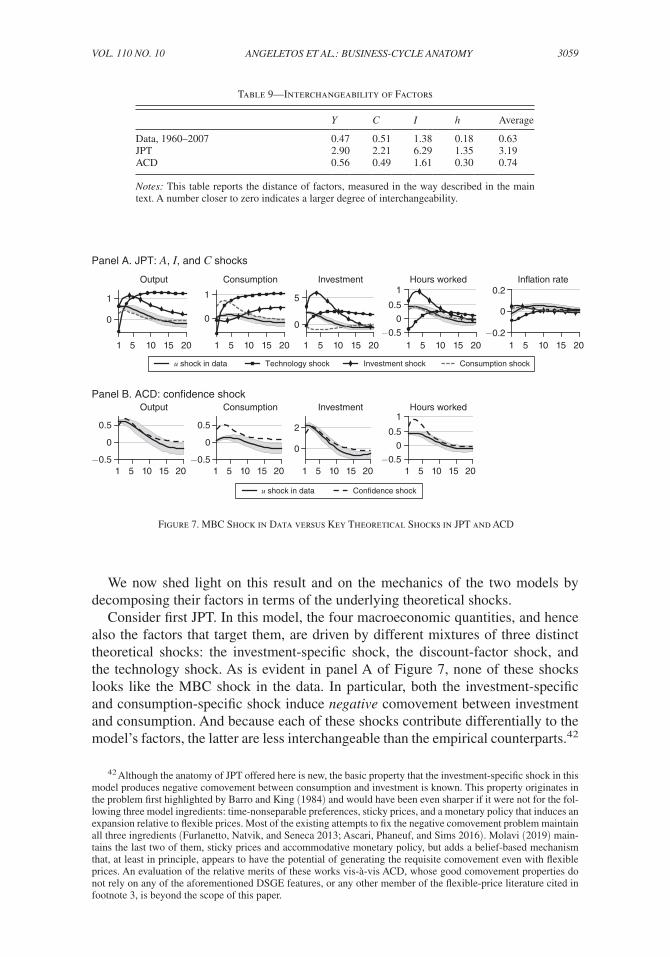
3059ANGELETOS ET AL.: BUSINESS-CYCLE ANATOMYVOL. 110 NO. 10
We now shed light on this result and on the mechanics of the two models by decomposing their factors in terms of the underlying theoretical shocks.
Consider first JPT. In this model, the four macroeconomic quantities, and hence also the factors that target them, are driven by different mixtures of three distinct theoretical shocks: the investment-specific shock, the discount-factor shock, and the technology shock. As is evident in panel A of Figure 7, none of these shocks looks like the MBC shock in the data. In particular, both the investment-specific and consumption-specific shock induce negative comovement between investment and consumption. And because each of these shocks contribute differentially to the model’s factors, the latter are less interchangeable than the empirical counterparts.42
42 Although the anatomy of JPT offered here is new, the basic property that the investment-specific shock in this model produces negative comovement between consumption and investment is known. This property originates in the problem first highlighted by Barro and King (1984) and would have been even sharper if it were not for the fol-lowing three model ingredients: time-nonseparable preferences, sticky prices, and a monetary policy that induces an expansion relative to flexible prices. Most of the existing attempts to fix the negative comovement problem maintain all three ingredients (Furlanetto, Natvik, and Seneca 2013; Ascari, Phaneuf, and Sims 2016). Molavi (2019) main-tains the last two of them, sticky prices and accommodative monetary policy, but adds a belief-based mechanism that, at least in principle, appears to have the potential of generating the requisite comovement even with flexible prices. An evaluation of the relative merits of these works vis-à-vis ACD, whose good comovement properties do not rely on any of the aforementioned DSGE features, or any other member of the flexible-price literature cited in footnote 3, is beyond the scope of this paper.
Table 9—Interchangeability of Factors
Y C I h Average
Data, 1960–2007 0.47 0.51 1.38 0.18 0.63JPT 2.90 2.21 6.29 1.35 3.19ACD 0.56 0.49 1.61 0.30 0.74
Notes: This table reports the distance of factors, measured in the way described in the main text. A number closer to zero indicates a larger degree of interchangeability.
Figure 7. MBC Shock in Data versus Key Theoretical Shocks in JPT and ACD
Output Consumption Investment Hours worked In�ation rate
Output Consumption Investment Hours worked
u shock in data Technology shock Investment shock Consumption shock
1 5 10 15 20 1 5 10 15 20 1 5 10 15 20 1 5 10 15 20
1 5 10 15 20 1 5 10 15 20 1 5 10 15 20 1 5 10 15 20 1 5 10 15 20
Con�dence shock
Panel A. JPT: A, I, and C shocks
Panel B. ACD: con�dence shock
u shock in data
1
0
1
00
51
0.5
−0.5
0
1
0.5
−0.5
0
0.2
−0.2
0
0.5
−0.5
0
0.5
−0.5
0
2
0

3060 THE AMERICAN ECONOMIC REVIEW OCTOBER 2020
Consider next ACD. In this model, all variables are driven, to a large extent, by the same shock, the confidence shock. As explained in more detail in Angeletos, Collard, and Dellas (2018), this shock is formalized as an extrinsic shock to higher-order beliefs but ultimately helps capture the following, broader mechanism: waves of optimism and pessimism about the short-term economic outlook without commensurate shifts in either TFP or the expectations of the long run.
Because optimism about the short run means that firms are bullish about their returns, the demand for both capital and labor goes up. And because such optimism entails relatively small changes in expected permanent income, it induces a rela-tively weak wealth effect on labor supply. This bypasses the problem faced by the literature on news shocks, in which beliefs regard persistent income changes and entail large wealth effects, and allows for a positive comovement between consump-tion, investment, and employment in the short run, even without the assistance of sticky prices and accommodative monetary policy.
The key observation for the present purposes, evident in panel B of Figure 7, is that this shock is quite similar to the MBC shock in the data, in terms of comove-ments and relative volatilities. This helps explain why the factors in ACD are almost as interchangeable as those in the data. Basically, this is because a bare-bones ver-sion of ACD, which shuts down all shocks except the confidence shock, achieves perfect interchangeability without a big sacrifice in terms of matching the MBC shock in the data, a property clearly not shared by any single-shock restriction of JPT and related DSGE models.
These lessons are robust to two additional exercises, which are reported in online Appendix Section J.2. In the first, we re-estimate JPT with the same frequency-domain method as that used in the estimation of ACD. In the second exercise, we re-estimate both JPT and ACD on the basis of our anatomy, namely by minimizing the distance of each model from the data in terms of the IRFs of the output, consumption, invest-ment, and hours to the four factors that target the same quantities. Both exercises help JPT produce more interchangeability, but the model still falls short of that found in the data as well as of that produced by the ACD model. The basic reason is that JPT does not contain a true structural shock/propagation mechanism like that seen in the data through our anatomy.
That said, the goal of these exercises is not to argue that ACD is superior to JPT, nor to question the importance of nominal rigidities, but rather to illustrate the prob-ing power of our empirical method and to give guidance to future research. In the same vein, we have applied our method to another important DSGE model, that of Christiano, Motto, and Rostagno (2014)—henceforth, CMR.
This model is on the forefront of a new strand of the DSGE literature that pays close attention to the real-financial nexus. Its main differences from the model used in Christiano, Eichenbaum, and Evans (2005) and Justiniano, Primiceri, and Tambalotti (2010) are the following three. First, it includes a financial friction that constrains investment, the latter been broadly defined to include consumer durables. Second, it contains a new structural shock (risk shock) that determines the severity of the financial friction.43 And third, it uses financial variables, most notably the
43 To be precise, this shock comes in nine flavors, depending on whether it hits the idiosyncratic volatility of firm returns with a lag of 0, 1, 2, … , 8 quarters.
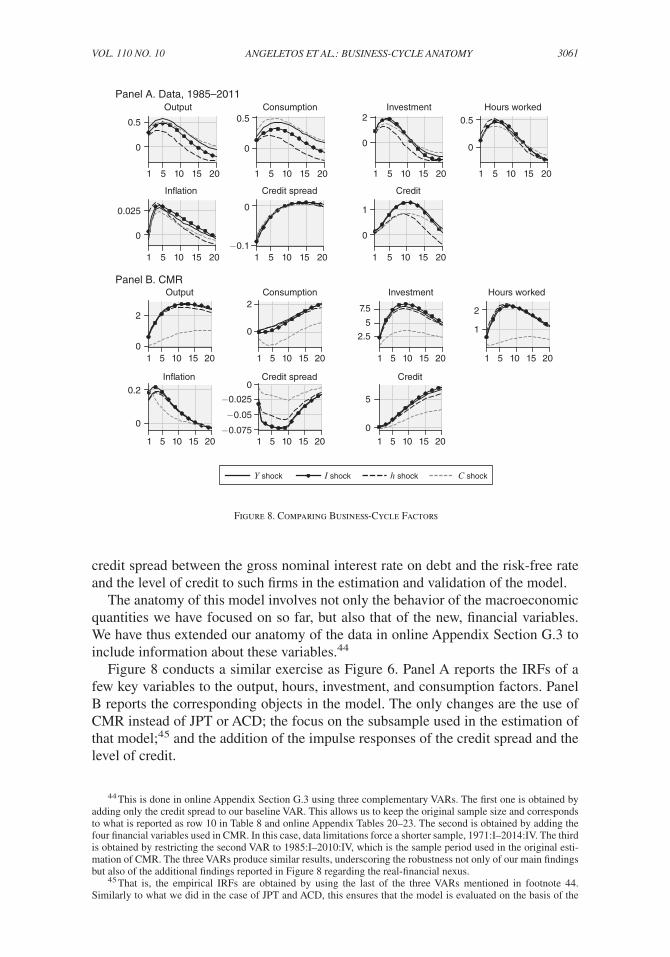
3061ANGELETOS ET AL.: BUSINESS-CYCLE ANATOMYVOL. 110 NO. 10
credit spread between the gross nominal interest rate on debt and the risk-free rate and the level of credit to such firms in the estimation and validation of the model.
The anatomy of this model involves not only the behavior of the macroeconomic quantities we have focused on so far, but also that of the new, financial variables. We have thus extended our anatomy of the data in online Appendix Section G.3 to include information about these variables.44
Figure 8 conducts a similar exercise as Figure 6. Panel A reports the IRFs of a few key variables to the output, hours, investment, and consumption factors. Panel B reports the corresponding objects in the model. The only changes are the use of CMR instead of JPT or ACD; the focus on the subsample used in the estimation of that model;45 and the addition of the impulse responses of the credit spread and the level of credit.
44 This is done in online Appendix Section G.3 using three complementary VARs. The first one is obtained by adding only the credit spread to our baseline VAR. This allows us to keep the original sample size and corresponds to what is reported as row 10 in Table 8 and online Appendix Tables 20–23. The second is obtained by adding the four financial variables used in CMR. In this case, data limitations force a shorter sample, 1971:I–2014:IV. The third is obtained by restricting the second VAR to 1985:I–2010:IV, which is the sample period used in the original esti-mation of CMR. The three VARs produce similar results, underscoring the robustness not only of our main findings but also of the additional findings reported in Figure 8 regarding the real-financial nexus.
45 That is, the empirical IRFs are obtained by using the last of the three VARs mentioned in footnote 44. Similarly to what we did in the case of JPT and ACD, this ensures that the model is evaluated on the basis of the
Figure 8. Comparing Business-Cycle Factors
1 5
0.5
0.025
0
0
0.5 2
0
22 7.5
2.5
5
0
0
0
2
0.2
1
0
−0.025
−0.05
5
0−0.075
1
0
0
−0.1
0
0.5
0
10 15 20
Output
1 5 10 15 20
Consumption
1 5 10 15 20
Investment
1 5 10 15 20
Hours worked
1 5 10 15 20
In�ation
1 15 10 15 20
Credit spread
5 10 15 20
Credit
1 5 10 15 20
Output
1 5 10 15 20
Consumption
1 5 10 15 20
Investment
1 5 10 15 20
Hours worked
1 5 10 15 20
In�ation
1 5 10 15 20
Credit spread
1 5 10 15 20
Credit
Y shock I shock h shock C shock
Panel A. Data, 1985–2011
Panel B. CMR

3062 THE AMERICAN ECONOMIC REVIEW OCTOBER 2020
The following patterns emerge. First, CMR improves upon JPT in terms of the interchangeability of the output, hours, and investment factors (thanks to having an even more dominant business-cycle driver), but it does worse in terms of both the response of consumption to the aforementioned factors and the response of all variables to the consumption factor. Second, CRM produces too much volatility and persistence compared to the data. Third, despite its use of a very flat Phillips curve and very sticky wages, CMR produces a much steeper relation between inflation and real economic activity than that seen in the data, underscoring its reliance on nominal rigidity. Finally, the model fails to capture the dynamics of the response of the credit spread to all of these factors: while in the data the credit spread appears to lead the MBC shock, in the sense that it peaks before the macroeconomic quantities, it does the opposite in the model.46
One may agree to disagree whether such model limitations are minor or signal a deeper problem with the propagation mechanism contained in mainstream DSGE models. Regardless, the exercises conducted in this section have illustrated the prob-ing power of our method in the context of medium-scale models.
VI. Conclusion
We have proposed a new strategy for dissecting macroeconomic time series and have used its findings to guide theory. The strategy involves the construction of a collection of reduced-form shocks, each of which maximizes the volatility of a par-ticular variable at particular frequencies. This yields a rich set of one-dimensional cuts of the macroeconomic data, which comprises our “anatomy.”
Prominent elements of this anatomy are the shocks that target the unemployment rate, GDP, hours worked, investment, consumption, and the output or unemploy-ment gap at the business-cycle frequencies. The near interchangeability of these objects in terms of IRFs motivates the concept of the MBC shock: we use this term to refer to the dynamic comovement patterns that are common to all these cuts of the data. These include a strong, positive, and transient comovement between the aforementioned quantities; little relation with either inflation or TFP at any horizon; and a disconnect between the short run and the long run.
The identified MBC shock can serve as an empirical template for the propagation mechanism that models of any size and complexity must contain. On this basis, we argued that the data speak against theories that seek to attribute the bulk of the business cycle to any of the following forces: technology shocks; financial, uncer-tainty, and other shocks that matter primarily by affecting aggregate TFP; news about medium- to long-run productivity prospects; and inflationary demand shocks. We further showed that our approach helps detect flaws in state-of-the-art DSGE
period used in its estimation. But as already mentioned, the empirical patterns themselves are robust to the longer period spanned by our baseline specification.
46 The excessive persistence appears to be the product of the model’s reliance on very high adjustment costs for investment and very persistent shocks. The property that the business cycle leads, rather than lags, the credit spread appears to be driven by the model’s reliance on a number of news shocks, which have a relatively more pronounced and front-loaded effect on investment, hours, and output than on the credit spread. And the inability to generate the requisite comovement between consumption and investment, or consumption and employment, echoes our earlier discussion of this issue within the context of JPT and the broader DSGE literature.

3063ANGELETOS ET AL.: BUSINESS-CYCLE ANATOMYVOL. 110 NO. 10
models that could have otherwise gone unnoticed, most notably the lack of sufficient interchangeability in the sense described above.
We interpret these findings as signals of deficiency in the propagation mechanism contained in mainstream macroeconomic models, and as support for theories aimed at accommodating demand-driven cycles without a strict reliance on nominal rigid-ities. We hope that the characterization of the data performed in the present paper will stimulate further research in this direction, or otherwise guide macroeconomic theory.
Appendix
A. Data
The data are from the Federal Reserve Economic Database (FRED). TFP corre-sponds to the TFP time series corrected for utilization produced by Fernald (2012) (downloaded 2016). Tables A1 and A2 describe the original data and the transfor-mations used in our VARs. Table A3 reports the raw (unconditional) correlations over the business-cycle frequencies.
B. Interchangeability in the Time Series
In the main text we emphasized the interchangeability of the various facets of the MBC shock in terms of IRFs. Figure B1 shows that a similar interchangeability property is present in terms of the time series generated by the reduced-form shocks. Each row in this figure reports, for each one of the key macroeconomic quantities, the scatterplot of that variable as predicted by the Y , I , C , and h shocks against its value as predicted by the unemployment shock. Table 3 summarizes the information contained in this figure in terms of correlations.
C. Application to News Shocks
In this section, we use our method to identify news shocks and examine how their properties, in particular their contribution to business cycles, vary with the size of the VAR used to identify the shocks. This serves two purposes. It sheds light on the source of the difference reported in the main text between our findings and those of Beaudry and Portier (2006). And it provides yet another example of the usefulness of our method outside the realm of one-shock representations of the business cycle, in particular, in the context of semistructural explorations.
The exercise conducted here is based on the premise that the vast majority, if not all, of the TFP fluctuations at all frequencies can be accounted for by two structural shocks: an unanticipated, permanent shock and a news shock. The former affects TFP both in the short and the long run, while the latter does not have an effect on impact.47
47 One may object to the assumption of only two TFP shocks, on the basis, for instance, that the “right” model features multiple news shocks, each one corresponding to different horizons at which TFP is expected to change.

3064 THE AMERICAN ECONOMIC REVIEW OCTOBER 2020
As explained in Section IV, the accommodation of these two structural shocks complicates the interpretation of the empirical MBC shock and in particular of its disconnect from the long run: this disconnect is consistent with models in which the two structural shocks under consideration have significant but offsetting effects on unemployment in the short run. Still, insofar as only these two shocks drive TFP, and regardless of how many other shocks may drive unemployment, we can identify the news shock and its business-cycle contribution as follows.
We first construct, via our method, the two empirical shocks that have the maximal contribution to the volatility of TFP in the long-run and the business-cycle frequen-cies ( 80−∞ and 6−32 quarters, respectively). Denote these by s t 1 and s t 2 , respectively. These shocks do not have a structural interpretation but are linear combinations of
But this is a slippery road that ultimately leads one to give up hope on “ atheoretic” endeavors and, instead, commit to a particular, fully specified model. Clearly, each approach has its strengths and limitations. We follow the one approach here and the other in Section IV.
Table A1—Description of Data
Data Mnemonic Frequency Transform
Real gross domestic product per capita A939RX0Q048SBEA Q —Gross domestic product GDP Q —Gross domestic product: implicit price deflator GDPDEF Q —Share of GDP: personal consumption expenditures: nondurable goods
DNDGRE1Q156NBEA Q —
Share of GDP: personal consumption expenditures: services
DSERRE1Q156NBEA Q —
Share of GDP: personal consumption expenditures: durable goods
DDURRE1Q156NBEA Q —
Share of GDP: gross private domestic investment A006RE1Q156NBEA Q —Nonfarm business sector: real output per hour of all persons OPHNFB Q —Nonfarm business sector: labor share PRS85006173 Q —Nonfarm business sector: average weekly hours PRS85006023 Q —Civilian non-institutional population CNP16OV M EoPCivilian unemployment rate UNRATE M AveEffective federal funds rate FEDFUNDS M AveTotal factor productivity (growth rate) DTFPu Q —
Note: Q: Quarterly, M: Monthly, EoP: end of period, Ave: quarterly average.
Table A2—Variables in the VARs
Real GDP per capital Y = 100 × log(A939RX0Q048SBEA)Real consumption per capita C = 100 × log((DNDGRE1Q156NBEA
+ DSERRE1Q156NBEA) × A939RX0Q048SBEA)
Real investment per capita I = 100 × log((DDURRE1Q156NBEA + A006RE1Q156NBEA) × A939RX0Q048SBEA)
Hours worked h = 100 × log(PRS85006023 × CE16OV/CNP16OV)Inflation rate π = 100 × log(GDPDEF/GDPDEF(−1))Interest rate R = FEDFUNDS/4
Productivity (NFB) y/h = 100 × log(OPHNFB)Labor share wh/y = 100 × log(PRS85006173)TFP TFP = log(cumulative sum (DTFPu/4))
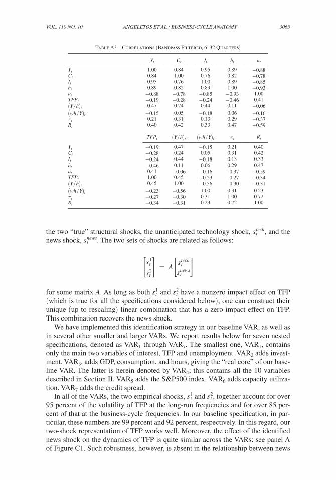
3065ANGELETOS ET AL.: BUSINESS-CYCLE ANATOMYVOL. 110 NO. 10
the two “true” structural shocks, the unanticipated technology shock, s t tech , and the news shock, s t news . The two sets of shocks are related as follows:
[ s t 1
s t 2 ] = A [ s t
tech s t news
]
for some matrix A . As long as both s t 1 and s t 2 have a nonzero impact effect on TFP (which is true for all the specifications considered below), one can construct their unique (up to rescaling) linear combination that has a zero impact effect on TFP. This combination recovers the news shock.
We have implemented this identification strategy in our baseline VAR, as well as in several other smaller and larger VARs. We report results below for seven nested specifications, denoted as VAR 1 through VAR 7 . The smallest one, VAR 1 , contains only the main two variables of interest, TFP and unemployment. VAR 2 adds invest-ment. VAR 3 , adds GDP, consumption, and hours, giving the “real core” of our base-line VAR. The latter is herein denoted by VAR 4 ; this contains all the 10 variables described in Section II. VAR 5 adds the S&P500 index. VAR 6 adds capacity utiliza-tion. VAR 7 adds the credit spread.
In all of the VARs, the two empirical shocks, s t 1 and s t 2 , together account for over 95 percent of the volatility of TFP at the long-run frequencies and for over 85 per-cent of that at the business-cycle frequencies. In our baseline specification, in par-ticular, these numbers are 99 percent and 92 percent, respectively. In this regard, our two-shock representation of TFP works well. Moreover, the effect of the identified news shock on the dynamics of TFP is quite similar across the VARs: see panel A of Figure C1. Such robustness, however, is absent in the relationship between news
Table A3—Correlations (Bandpass Filtered, 6–32 Quarters)
Y t C t I t h t u t
Y t 1.00 0.84 0.95 0.89 −0.88 C t 0.84 1.00 0.76 0.82 −0.78 I t 0.95 0.76 1.00 0.89 −0.85 h t 0.89 0.82 0.89 1.00 −0.93 u t −0.88 −0.78 −0.85 −0.93 1.00 TF P t −0.19 −0.28 −0.24 −0.46 0.41 (Y / h) t 0.47 0.24 0.44 0.11 −0.06 (wh / Y) t −0.15 0.05 −0.18 0.06 −0.16 π t 0.21 0.31 0.13 0.29 −0.37 R t 0.40 0.42 0.33 0.47 −0.59
TF P t (Y / h) t (wh / Y) t π t R t
Y t −0.19 0.47 −0.15 0.21 0.40 C t −0.28 0.24 0.05 0.31 0.42 I t −0.24 0.44 −0.18 0.13 0.33 h t −0.46 0.11 0.06 0.29 0.47 u t 0.41 −0.06 −0.16 −0.37 −0.59 TF P t 1.00 0.45 −0.23 −0.27 −0.34 (Y / h) t 0.45 1.00 −0.56 −0.30 −0.31 (wh / Y) t −0.23 −0.56 1.00 0.31 0.23 π t −0.27 −0.30 0.31 1.00 0.72 R t −0.34 −0.31 0.23 0.72 1.00

3066 THE AMERICAN ECONOMIC REVIEW OCTOBER 2020
shocks and unemployment fluctuations; see panel B of Figure C1. In particular, the news shock switches from being strongly expansionary in the smallest VAR to being slightly contractionary in the largest VAR.
Figure C2 presents this sensitivity in terms of the contribution of the identified news shock to the volatility of unemployment at the business-cycle frequencies. On the horizontal axis, we vary the size of the VAR used in the construction of s t 1 and s t 2 and, thereby, of the news shock: as we move from left to right, we progressively add more data and, accordingly, increase the size of the VAR from 2 variables to a total of 13.
Figure C2 speaks for itself: as more information (in the form of the additional variables) is incorporated, the estimated contribution of the news shock declines dramatically, stabilizing at around 11 percent in the last four specifications. In our baseline specification, the number is 13 percent.
Y s
hock
Y s
hock
Y s
hock
Y s
hock
Y s
hock
C s
hock
C s
hock
C s
hock
C s
hock
C s
hock
I sh
ock
I sh
ock
I sh
ock
I sh
ock
I sh
ock
h sh
ock
u shock u shock u shock u shock
u shock u shock u shock u shock
u shock u shock u shock u shock
u shock u shock u shock u shock
h sh
ock
h sh
ock
h sh
ock
h sh
ock
Panel A. Unemployment
Panel B. Output
Panel C. Hours worked
Panel D. Investment
Panel E. Consumption
0.50
0
0
0
2
1
0
−1
−2
12
0−1−2
1
0
−1
−2
10
−1
1
0
−1−2
5
0
−5
5
0
−5
10
−1
−2
50
−5−10
1
0
−1
−2
0
2
−2
−0.5
−0.5
−1
−1
−10 −5 5
0−2 2
0−1 1 0−1 1 0−1 1 0−1 1
0−2 2 0−2 2 0−2 2
0−10 −5 5 0−10 −5 5 0−10 −5 5
0.5 0−0.5−1 0.5 0−0.5−1 0.5 0−0.5−1 0.5
0 1−0.5
−0.5
0.5
0−0.5
0.5
1
−1
0−0.5
0.51
−1
0
−0.5
0.5
1
0
0.50 1−0.5 0.50 1−0.5 0.50 1−0.5 0.5
10
−10
5
−50
0.5
0
−0.5
−1
0.5
0−0.5
−1
Figure B1. The Various Facets of the MBC Shock, Scatterplots

3067ANGELETOS ET AL.: BUSINESS-CYCLE ANATOMYVOL. 110 NO. 10
Due to the well-known potential fragility of results from small VARs (Forni, Gambetti, and Sala 2019), we trust more the results from the medium and larger ones, especially because size ceases to matter after a certain size. Larger VARs con-tain more information, while smaller ones may mechanically attribute a larger share of the business cycle to the news shock.
To illustrate the latter point, consider VAR 1 . In this specification, the news shock accounts for 97 percent of the short-run fluctuations in unemployment. Why? In a two variables–two shocks specification, s t tech and s t news must together account for all of the fluctuations in unemployment. Due to the assumption that s t tech is the only shock that has an immediate, impact effect on TFP, s t tech is closely associated with actual TFP in the short run. But as we have established, TFP is nearly orthogonal to unemployment at the business-cycle frequencies (and beyond). It then follows that s t tech can account for only a trivial fraction of the unemployment fluctuations, which leaves s t news as the only shock to explain unemployment fluctuations. In short, this VAR mechanically attributes a large fraction of the business cycle to the news shock, simply because the only other allowed shock is a “dead horse” to start with.
Panel A. TFP
Quarters Quarters
Panel B. Unemployment
0.4
0
0
−0.1
−0.2
−0.3
−0.4
1 5 10 15 20 1 5 10 15 20
0.3
0.2
0.1
VAR1 VAR2 VAR3 VAR4 VAR5 VAR6 VAR7
0
20
40
60
80
100
VAR1 VAR2 VAR3 VAR4 VAR5 VAR6 VAR7
Figure C1. IRF of TFP and Unemployment to News Shock
Note: Shaded area: 68 percent HPDI for VAR 4 (baseline).
Figure C2. Variance Contribution of News Shock to Unemployment
Notes: Contribution of news shock to unemployment at business-cycle frequencies. Gray line gives median, upper, and lower black lines give 68 percent HPDI. VAR 1 = {u ,TFP } , VAR 2 = VAR 1 ∪ {I} , VAR 3 = VAR 2 ∪ {Y, C, h} , VAR 4 = Baseline VAR, VAR 5 = VAR 4 ∪ {SP500} , VAR 6 = VAR 5 ∪ { utilization }, VAR 7 = VAR 6 ∪ { credit spread } .

3068 THE AMERICAN ECONOMIC REVIEW OCTOBER 2020
As we move to larger VARs, we add more data but also more shocks that can con-tribute to the fluctuations in unemployment. So the role of news is bound to wither. Figure C2 shows that the decline is precipitous at first, but stabilizes once we reach the baseline specification.
This helps shed light on the main reason why our results differ from those in Beaudry and Portier: we use larger VARs than they do. Another part of the differ-ence comes from using different identifying assumptions.
The exercise conducted here also serves another important purpose. Namely, it helps showcase the usefulness of our approach in the realm of multishock models without a need for the explicit intermediation of a particular, fully specified model. The key is to drop the exclusive focus on the MBC shock and include other fea-tures of the anatomy, here, for instance, the shocks that target TFP in the short and the long run, and to utilize the cross-equation restrictions associated with them. As shown in Section V, the same procedure also proves very effective in the context of fully structural endeavors.
REFERENCES
Angeletos, George-Marios, Fabrice Collard, and Harris Dellas. 2015. “Quantifying Confidence.” NBER Working Paper 20807.
Angeletos, George-Marios, Fabrice Collard, and Harris Dellas. 2018. “Quantifying Confidence.” Econometrica 86 (5): 1689–1726.
Angeletos, George-Marios, Fabrice Collard, and Harris Dellas. 2020. “Replication Data for: Busi-ness-Cycle Anatomy.” American Economic Association [publisher], Inter-university Consortium for Political and Social Research [distributor]. https://doi.org/10.3886/E118082V1.
Angeletos, George-Marios, and Jennifer La’O. 2010. “Noisy Business Cycles.” In NBER Macroeco-nomics Annual 2009, Vol. 24, edited by Daron Acemoglu, Kenneth Rogoff, and Michael Woodford, 319–78. Chicago: University of Chicago Press.
Angeletos, George-Marios, and Jennifer La’O. 2013. “Sentiments.” Econometrica 81 (2): 739–79.Angeletos, George-Marios, and Chen Lian. 2020. "Confidence and the Propagation of Demand
Shocks." NBER Working Paper 27702.Arellano, Cristina, Yan Bai, and Patrick J. Kehoe. 2019. “Financial Frictions and Fluctuations in Vol-
atility.” Journal of Political Economy 127 (5): 2049–103. Ascari, Guido, Louis Phaneuf, and Eric Sims. 2016. “Business Cycles, Investment Shocks, and the
‘Barro-King’ Curse.” NBER Working Paper 22941.Atkeson, Andrew, and Lee E. Ohanian. 2001. “Are Phillips Curves Useful for Forecasting Inflation?”
Federal Reserve Bank of Minneapolis Quarterly Review 25 (1): 2–11.Bai, Yan, José-Victor Ríos-Rull, and Kjetil Storesletten. 2017. “Demand Shocks as Productivity
Shocks.” Unpublished.Barro, Robert J., and Robert G. King. 1984. “Time-Separable Preferences and Intertemporal-Substitu-
tion Models of Business Cycles.” Quarterly Journal of Economics 99 (4): 817–39.Barsky, Robert B., and Eric R. Sims. 2011. “News Shocks and Business Cycles.” Journal of Monetary
Economics 58 (3): 273–89.Beaudry, Paul, Dana Galizia, and Franck Portier. 2018. “Reconciling Hayek’s and Keynes’ Views of
Recessions.” Review of Economic Studies 85 (1): 119–56. Beaudry, Paul, Dana Galizia, and Franck Portier. 2020. “Putting the Cycle Back into Business Cycle
Analysis.” American Economic Review 110 (1): 1–47Beaudry, Paul, and Franck Portier. 2006. “Stock Prices, News, and Economic Fluctuations.” American
Economic Review 96 (4): 1293–307. Beaudry, Paul, and Franck Portier. 2014. “Understanding Noninflationary Demand-Driven Busi-
ness Cycles.” In NBER Macroeconomics Annual 2013, Vol. 28, edited by Jonathan A. Parker and Michael Woodford, 69–130. Chicago: University of Chicago Press.
Beaudry, Paul, and Franck Portier. 2018. “Real Keynesian Models and Sticky Prices.” NBER Work-ing Paper 24223.
Benhabib, Jess, and Roger E. A. Farmer. 1994. “Indeterminacy and Increasing Returns.” Journal of Economic Theory 63 (1): 19–41.

3069ANGELETOS ET AL.: BUSINESS-CYCLE ANATOMYVOL. 110 NO. 10
Benhabib, Jess, Pengfei Wang, and Yi Wen. 2015. “Sentiments and Aggregate Demand Fluctuations.” Econometrica 83 (2): 549–85.
Blanchard, Olivier Jean, and Danny Quah. 1989. “The Dynamic Effects of Aggregate Demand and Supply Disturbances.” American Economic Review 79 (4): 655–73.
Bloom, Nicholas, Max Floetotto, Nir Jaimovich, Itay Saporta-Eksten, and Stephen J. Terry. 2018. “Really Uncertain Business Cycles.” Econometrica 86 (3): 1031–65.
Canova, Fabio. 2020. “FAQ: How Do I Extract the Output Gap?” Unpublished.Chahrour, Ryan, and Kyle Jurado. 2018. “News or Noise? The Missing Link.” American Economic
Review 108 (7): 1702–36.Christiano, Lawrence J., Martin Eichenbaum, and Charles L. Evans. 2005. “Nominal Rigidities and
the Dynamic Effects of a Shock to Monetary Policy.” Journal of Political Economy 113 (1): 1–45.Christiano, Lawrence J., and Terry J. Fitzgerald. 2003. “The Band Pass Filter.” International Eco-
nomic Review 44 (2): 435–65. Christiano, Lawrence J., Roberto Motto, and Massimo Rostagno. 2014. “Risk Shocks.” American
Economic Review 104 (1): 27–65.Cochrane, John H. 1994. “Shocks.” Carnegie-Rochester Conference Series on Public Policy 41: 295–
364.Debortoli, Davide, Jordi Galí, and Luca Gambetti. 2019. “On the Empirical (Ir)Relevance of the Zero
Lower Bound Constraint.” NBER Working Paper 25820.Diamond, Peter A. 1982. “Aggregate Demand Management in Search Equilibrium.” Journal of Politi-
cal Economy 90 (5): 881–94.Dotsey, Michael, Shigeru Fujita, and Tom Stark. 2018. “Do Phillips Curves Conditionally Help to
Forecast Inflation?” International Journal of Central Banking 14 (4): 43–92.Eusepi, Stefano, and Bruce Preston. 2015. “Consumption Heterogeneity, Employment Dynamics and
Macroeconomic Co-Movement.” Journal of Monetary Economics 71: 13–32.Faust, John. 1998. “The Robustness of Identified VAR Conclusions about Money.” Carnegie-Roches-
ter Conference Series on Public Policy 49: 207–44.Fernald, John. 2012. “A Quarterly, Utilization-Adjusted Series on Total Factor Productivity.” Federal
Reserve Bank of San Francisco Working Paper 2012-19.Forni, Mario, Luca Gambetti, and Luca Sala. 2019. “Structural VARs and Noninvertible Macroeco-
nomic Models.” Journal of Applied Econometrics 34 (2): 221–46.Furlanetto, Francesco, Gisle J. Natvik, and Martin Seneca. 2013. “Investment Shocks and Macroeco-
nomic Co-Movement.” Journal of Macroeconomics 37: 208–16.Galí, Jordi. 1999. “Technology, Employment, and the Business Cycle: Do Technology Shocks Explain
Aggregate Fluctuations?” American Economic Review 89 (1): 249–71.Galí, Jordi, and Mark Gertler. 1999. “Inflation Dynamics: A Structural Econometric Analysis.” Jour-
nal of Monetary Economics 44 (2): 195–222.Golosov, Mikhail, and Guido Menzio. 2015. “Agency Business Cycles.” NBER Working Paper 21743.Guesnerie, Roger, and Michael Woodford. 1993. “Endogenous Fluctuations.” In Advances in Eco-
nomic Theory: Sixth World Congress, Vol. 2, edited by Jean-Jacques Laffont, 289–412. Cambridge, UK: Cambridge University Press.
Huo, Zhen, and Naoki Takayama. 2015. “Higher Order Beliefs, Confidence, and Business Cycles.” Unpublished.
Huo, Zhen, and Jose-Victor Rios-Rull. Forthcoming. “Demand Induced Fluctuations.” Review of Eco-nomic Dynamics.
Ilut, Cosmin, and Hikaru Saijo. 2018. “Learning, Confidence, and Business Cycles.” Unpublished.Jaimovich, Nir, and Sergio Rebelo. 2009. “Can News about the Future Drive the Business Cycle?”
American Economic Review 99 (4): 1097–1118.Justiniano, Alejandro, Giorgio E. Primiceri, and Andrea Tambalotti. 2010. “Investment Shocks and
Business Cycles.” Journal of Monetary Economics 57 (2): 132–45.Koop, Gary. 2003. Bayesian Econometrics. Hoboken, NJ: John Wiley & Sons. Kydland, Finn E., and Edward C. Prescott. 1982. “Time to Build and Aggregate Fluctuations.” Econo-
metrica 50 (6): 1345–70.Lorenzoni, Guido. 2009. “A Theory of Demand Shocks.” American Economic Review 99 (5): 2050–84.Lucas, Robert E., Jr. 1975. “An Equilibrium Model of the Business Cycle.” Journal of Political Econ-
omy 83 (6): 1113–44.Lucas, Robert E., Jr. 1977. “Understanding Business Cycles.” Carnegie-Rochester Conference Series
on Public Policy 5: 7–29.Mavroeidis, Sophocles, Mikkel Plagborg-Møller, and James H. Stock. 2014. “Empirical Evidence on
Inflation Expectations in the New Keynesian Phillips Curve.” Journal of Economic Literature 52 (1): 124–88.

3070 THE AMERICAN ECONOMIC REVIEW OCTOBER 2020
McLeay, Michael, and Silvana Tenreyro. 2020. “Optimal Inflation and the Identification of the Phillips Curve.” In NBER Macroeconomics Annual 2019, Vol. 34, edited by Martin S. Eichenbaum, Erik Hurst, and Jonathan A. Parker, 199–255. Chicago: University of Chicago Press.
Molavi, Pooya. 2019. “Macroeconomics with Learning and Misspecification: A General Theory and Applications.” Unpublished.
Neville, Francis, Michael T. Owyang, Jennifer E. Roush, and Riccardo DiCecio. 2014. “A Flexible Finite-Horizon Alternative to Long-Run Restrictions with an Application to Technology Shocks.” Review of Economics and Statistics 96 (4): 638–47.
Ramey, Valerie A. 2016. “Macroeconomic Shocks and Their Propagation.” In Handbook of Macroeco-nomics, Vol. 2A, edited by John B. Taylor and Harald Uhlig, 71–162. Amsterdam: Elsevier.
Smets, Frank, and Rafael Wouters. 2007. “Shocks and Frictions in US Business Cycles: A Bayesian DSGE Approach.” American Economic Review 97 (3): 586–606.
Stock, James H., and Mark W. Watson. 1999. “Business Cycle Fluctuations in US Macroeconomic Time Series.” In Handbook of Macroeconomics, Vol. 1A, edited by John B. Taylor and Michael Woodford, 3–64. Amsterdam: Elsevier.
Stock, James H., and Mark W. Watson. 2007. “Why Has U.S. Inflation Become Harder to Forecast?” Journal of Money, Credit, and Banking 39 (S1): 3–33.
Stock, James H., and Mark W. Watson. 2009. “Phillips Curve Inflation Forecasts.” In Understanding Inflation and the Implications for Monetary Policy: A Phillips Curve Retrospective, edited by Jeff Fuhrer et al., 101–86. Cambridge, MA: MIT Press.
Uhlig, Harald. 2003. “What Moves Real GNP?” Unpublished.