Frank M. Fossen

Risky Earnings, Taxation and Entrepreneurial Choice: A Microeconometric Model for Germany

SOEPpapers on Multidisciplinary Panel Data Research

Berlin, August 2007

SOEPpapers on Multidisciplinary Panel Data Research at DIW Berlin

This series presents research findings based either directly on data from the German Socio-Economic Panel Study (SOEP) or using SOEP data as part of an internationally comparable data set (e.g. CNEF, ECHP, LIS, LWS, CHER/PACO). SOEP is a truly multidisciplinary household panel study covering a wide range of social and behavioral sciences: economics, sociology, psychology, survey methodology, econometrics and applied statistics, educational science, political science, public health, behavioral genetics, demography, geography, and sport science. The decision to publish a submission in SOEPpapers is made by a board of editors chosen by the DIW Berlin to represent the wide range of disciplines covered by SOEP. There is no external referee process and papers are either accepted or rejected without revision. Papers appear in this series as works in progress and may also appear elsewhere. They often represent preliminary studies and are circulated to encourage discussion. Citation of such a paper should account for its provisional character. A revised version may be requested from the author directly. Any opinions expressed in this series are those of the author(s) and not those of DIW Berlin. Research disseminated by DIW Berlin may include views on public policy issues, but the institute itself takes no institutional policy positions. The SOEPpapers are available at http://www.diw.de/soeppapers Editors:

Georg Meran (Vice President DIW Berlin) Gert G. Wagner (Social Sciences) Joachim R. Frick (Empirical Economics) Jürgen Schupp (Sociology)

Conchita D’Ambrosio (Welfare Economics) Christoph Breuer (Sport Science, DIW Research Professor) Anita I. Drever (Geography) Frieder R. Lang (Psychology, DIW Research Professor) Jörg-Peter Schräpler (Survey Methodology) C. Katharina Spieß (Educational Science) Martin Spieß (Statistical Modelling) Viktor Steiner (Public Economics, Department Head DIW Berlin) Alan S. Zuckerman (Political Science, DIW Research Professor) ISSN: 1864-6689

German Socio-Economic Panel Study (SOEP) DIW Berlin Mohrenstrasse 58 10117 Berlin, Germany Contact: Uta Rahmann | urahmann@diw.de

Risky Earnings, Taxation and Entrepreneurial Choice –

A Microeconometric Model for Germany1

Frank M. Fossen

DIW Berlin

(e-mail: ffossen@diw.de)

July 9th, 2007

Abstract:

Which role do individual income prospects play in the decision to be an entrepreneur rather

than an employee? In a model of occupational choice, higher expected after-tax earnings

attract people to self-employment, while more risky net earnings deter risk-averse individuals.

In this paper I analyse the expected value and variance of income in self-employment and

dependent employment empirically, accounting for selection. Based on this analysis,

structural models of self-employment entry and exit under risk are estimated, which include a

standard risk aversion parameter. The model predicts that the German income tax reduction of

2000 induced smaller exit rates out of self-employment for men and smaller entry rates for

women.

JEL classification: J23, H24, D81, C51

Keywords: Entrepreneurship, Risk, Returns to Self-Employment, Taxation

1 Acknowledgements: I would like to thank the Deutsche Forschungsgemeinschaft (DFG, German Research Foundation) for financial support of the project “Tax Policy and Entrepreneurial Choice” (STE 681/7-1). Furthermore, I am grateful to Viktor Steiner and colleagues at the German Institute for Economic Research (DIW Berlin) for valuable advice and helpful comments. The usual disclaimer applies.

1 Introduction

The factors that induce people to start up or close small entrepreneurial ventures have

received increasing attention among academics and politicians alike recently. Entrepreneurs

are agued to introduce new products and new technology, enter new markets and keep the

market economy innovative, dynamic and competitive. Small firms are also often regarded as

an engine for the creation of new jobs, which has made entrepreneurship a key topic in

countries with high unemployment. In Germany, for example, slow economic growth and

high unemployment have been attributed to the lack of start-ups: “In Germany, too few

companies are being born. [..] What is lacking are [..] small entrepreneurial start-ups that have

been the secret of so much development in Britain, America and elsewhere” (The Economist

2006). Consequently, governments in Germany and elsewhere have implemented various

policies to promote entrepreneurship. As among the various potential determinants of

entrepreneurship, taxation is under direct control of the government, tax policy is frequently

suggested as an instrument to stimulate entrepreneurship.

The dominating research approach to analyse the impact of income taxation on

entrepreneurial choice has been the ex-post analysis of certain tax reforms (recent studies

include Moore 2004; Parker 2003; Bruce 2002; Cullen and Gordon 2002; Georgellis and Wall

2002; Bruce 2000; Schuetze 2000; Fossen and Steiner 2006; see Schuetze and Bruce 2004 for

a survey). This branch of research brought about mixed results about the responsiveness of

entrepreneurial choice to taxation. These ex-post studies are however only of limited

applicability for the evaluation of future tax reform options ex-ante, as often demanded by

policy makers. This is a motivation for developing and estimating a structural model of

entrepreneurial choice.

Income taxation may influence entrepreneurial choice, which is understood here as the

decision between dependent employment and self-employment, through its impact on net

(after-tax) earnings in both alternatives. Thus, to understand the effect of income taxation, it is

necessary to analyse the influence of net earnings on this decision. In models of

entrepreneurship as an occupational choice, the probability of choosing self-employment can

be represented as a function of the differential in expected earnings from self-employment and

wage employment. Empirical studies analysing this earnings differential include Fraser and

Greene (2006) and Taylor (1996), who confirmed that higher expected earnings in self-

employment relative to paid employment significantly increase the probability of becoming

self-employed, Dolton and Makepeace (1990) and Rees and Shah (1986), who also found a

1

positive, but insignificant effect, and Hamilton (2000), who in contrast concluded that factors

other than earnings induce people to become self-employed. All these studies only looked at

gross earnings, however, so they did not consider the impact of taxes.

Not only preferences of individuals over net returns, but also over risk may play a role in

entrepreneurial choice, as higher risk associated with income from self-employment may

deter risk-averse individuals from choosing this option. This idea is related to Kanbur (1982)

and Khilstrom and Laffont (1979) who modelled entrepreneurial choice as trading off risk and

returns. They suggested that the less risk-averse become entrepreneurs and may receive a risk

premium as compensation of the greater variance of their earnings. The historical roots of

these models are in the work of Knight (1921), according to whom the central role of the

entrepreneur is to bear risks. Recent empirical works found evidence that risk attitudes play a

significant role in the decision to become self-employed (Cramer et al. 2002; Caliendo,

Fossen and Kritikos 2006).

Taxation alters both the expected value and the variance of net earnings. A progressive

income tax reduces expected net returns of a risky project such as starting up a business

(Gentry and Hubbard 2000), but also flattens the stream of net returns over years, which

reduces the risk associated with self-employment (Domar and Musgrave 1944). The first

effect may discourage, but the second may encourage an entrepreneurial venture. The overall

effect of taxation on entrepreneurial choice remains unclear as long as it is not understood to

what extent both the expected value of net income and the risk associated with it (in terms of

the variance) influence this choice.

A structural model is needed to approach this problem. Attempts to estimate a structural

model of entrepreneurial choice incorporating earnings and risk have been very rare. Rees and

Shah (1986) formulated a model of the probability of being self-employed assuming a utility

function with constant relative risk aversion, but used a much simplified model without an

explicit risk parameter in their empirical estimation. Pfeiffer and Pohlmeier (1992) specified a

similar model and actually estimated its parameters using the first waves of the German

Socio-Economic Panel (SOEP waves 1984-1989, limited to West Germany). They only

considered gross incomes, however, and left out the role of taxation, which is the main

motivation for this paper. Moreover, mean income and variance curves will be estimated

individually in this paper, and duration dependence will be controlled for in the transition

models (see section 3). Rosen and Willen (2002) used the Panel Study of Income Dynamics

and found that in comparison to wage employment, self-employment both comes with an

increase in mean yearly consumption and an increased variance of returns, which is consistent

2

with a risk premium for the self-employed. They used the measured level and variance of

income in the two occupational modes to asses a theoretical model of self-employment

choice, but came to the conclusion that the risk premium was too large to be rationalized by

conventional measures of risk aversion. A possible explanation may be that the authors used

yearly income and did not take into account that the self-employed work more weekly hours

on average than wage employees. They also only looked at gross incomes and neglected the

impact of taxes.

In this paper I develop a structural model of transition probabilities between dependent

employment and self-employment, which takes into account both expected net earnings and

net earnings variance in the two alternative employment states. These first and second

moments of random earnings are estimated empirically for both income from self-

employment and dependent employment, controlling for non-random selection into these

states. Not only one period’s income, but lifetime income matters for the significant decision

to enter or exit self-employment. This is taken into account by predicting the curves of future

expected earnings and earnings variance over each individual’s lifetime conditional on the

choice to be an entrepreneur or a wage worker. Summary statistics of these predicted curves

enter the structural transition models, which enables me to estimate the model parameters

empirically. These parameters include the standard Arrow-Pratt measure of relative risk

aversion, which can be related to results in the existing literature. The estimated model allows

calculating elasticities of the transition probabilities with respect to the expected value and the

variance of net income. To illustrate the results, the model is applied to simulate the effects of

the German Tax Reduction Act 2000 on the self-employment entry and exit rates.

The structural transition model is developed in section 2 of this paper, and translated into

empirical discrete time hazard rate models in section 3.1. Section 3.2 briefly introduces the

data. The methodology for the estimation of gross earnings and their variance, controlling for

selection, is described in sections 3.3 to 3.5. Sections 3.6 and 3.7 deal with the tax rate

function and the calculation of annuities. The empirical results are presented in section 4,

along with the simulation of the tax reform and a sensitivity analysis, and section 5 concludes.

2 The Structural Model

The model presented here is based on a binary representation of the decision to be self-

employed or dependently employed. In a given period, an individual i makes a rational choice

3

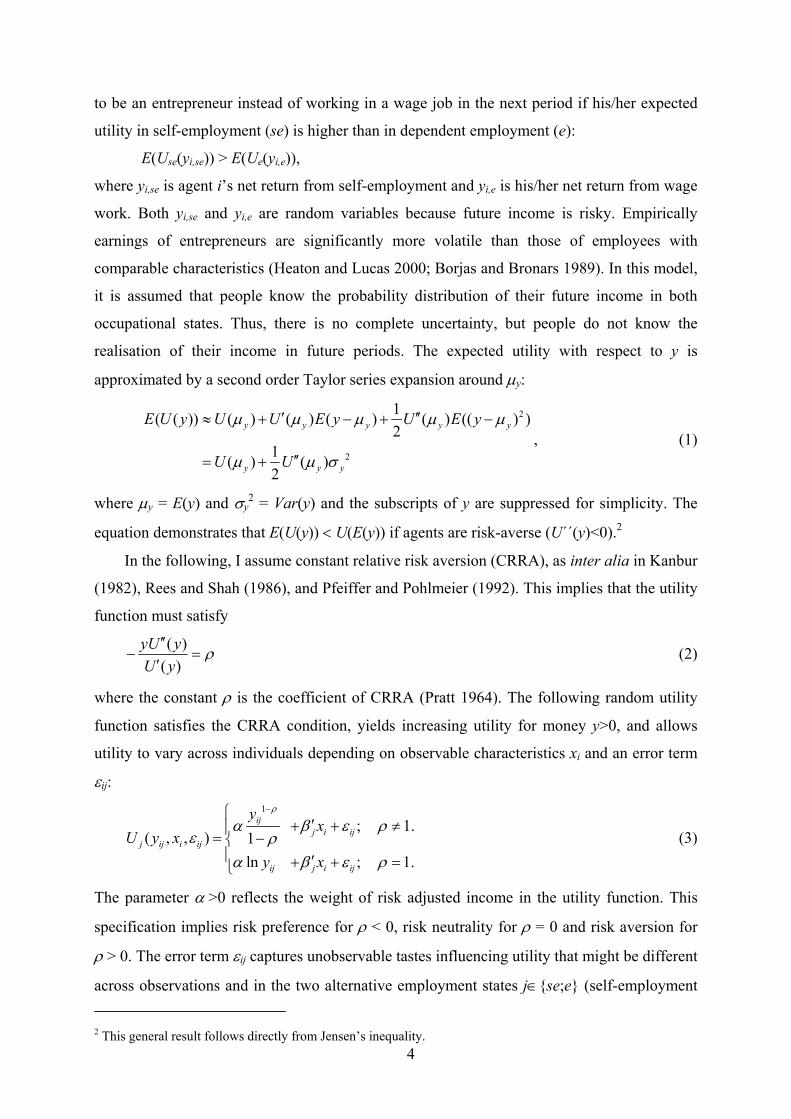
to be an entrepreneur instead of working in a wage job in the next period if his/her expected

utility in self-employment (se) is higher than in dependent employment (e):

E(Use(yi,se)) > E(Ue(yi,e)),

where yi,se is agent i’s net return from self-employment and yi,e is his/her net return from wage

work. Both yi,se and yi,e are random variables because future income is risky. Empirically

earnings of entrepreneurs are significantly more volatile than those of employees with

comparable characteristics (Heaton and Lucas 2000; Borjas and Bronars 1989). In this model,

it is assumed that people know the probability distribution of their future income in both

occupational states. Thus, there is no complete uncertainty, but people do not know the

realisation of their income in future periods. The expected utility with respect to y is

approximated by a second order Taylor series expansion around µy:

2

2

1( ( )) ( ) ( ) ( ) ( ) (( )2

1( ) ( )2

µ µ µ µ µ

µ µ σ

′ ′′≈ + − + −

′′= +

y y y y

y y y

E U y U U E y U E y

U U

)y

, (1)

where µy = E(y) and σy2 = Var(y) and the subscripts of y are suppressed for simplicity. The

equation demonstrates that E(U(y)) < U(E(y)) if agents are risk-averse (U´´(y)<0).2

In the following, I assume constant relative risk aversion (CRRA), as inter alia in Kanbur

(1982), Rees and Shah (1986), and Pfeiffer and Pohlmeier (1992). This implies that the utility

function must satisfy

( )( )

ρ′′

−′

yU yU y

= (2)

where the constant ρ is the coefficient of CRRA (Pratt 1964). The following random utility

function satisfies the CRRA condition, yields increasing utility for money y>0, and allows

utility to vary across individuals depending on observable characteristics xi and an error term

εij: 1

; 1( , , ) 1

ln ; 1.

ρ

α β ε ρε ρ

α β ε ρ

−′+ + ≠= −

′+ + =

ijj i ij

j ij i ij

ij j i ij

yx

U y xy x

.

(3)

The parameter α >0 reflects the weight of risk adjusted income in the utility function. This

specification implies risk preference for ρ < 0, risk neutrality for ρ = 0 and risk aversion for

ρ > 0. The error term εij captures unobservable tastes influencing utility that might be different

across observations and in the two alternative employment states j∈{se;e} (self-employment

42 This general result follows directly from Jensen’s inequality.

and dependent employment). These tastes are unobservable for the researcher and thus treated

as a random variable, but they are known to the individuals in the sample, in contrast to the

error in future earnings y. Unobserved factors influencing utility in self-employment might

include the desire to be independent (Taylor 1996) or the believe in the power of one’s own

actions (Evans and Leighton 1989). The first and second order partial derivations of U with

respect to y (suppressing subscripts j and i) are

1

1

2

; 1( , , )

; 1

; 1( , , )

; 1

ρ

ρ

α ρε

α ρ

αρ ρε

α ρ

−

−

− −

−

≠′ = =

.

.

.

.− ≠′′ = − =

yU y x

y

yU y x

y

(4)

Plugging U’’ into equation (1) yields expected utility with respect to y: 1

1 2

22

1 ; 11 2

( ( , , ))1ln ; 1.

2

ρρµ

α ρµ σ β ερ

ε

α µ σ β ε ρµ

−− −

′− + + − ≈

′− + +

yy y

y yy

x

E U y x

x

.ρ ≠

=

(5)

With α >0, the equation reflects that given expected earnings, for risk-averse agents expected

utility decreases with greater variance of earnings. For risk-neutral agents the variance does

not matter, and for risk-loving individuals, greater variance actually increases expected utility.

Taking the expectation with respect to the random earnings variable y did not remove the

utility error term ε.

As the agent chooses the employment state which gives him/her the highest utility, the

probability that agent i decides to be an entrepreneur in the next period is

Prob(se| yi,se, yi,e, xi) = Prob(E(Use(yi,se, xi, εi,se) > E(Ue(yi,e, xi, εi,e))

= Prob(εi,e - εi,se < α(V(yi,se) - V(yi,e)) + (βse - βe)´ xi)

= F(α(V(yi,se) - V(yi,e)) + β´xi) (6)

where β = βse - βe, F is the cumulative density function of the error term εi = εi,e - εi,se, and 1

1 2

22

1 ; 11 2

( )1ln ; 1.

2

ρρµ

ρµ σ ρρ

µ σ ρµ

−− −

− ≠

−= − =

yy y

ij

y yy

V y. (7)

can be interpreted as risk adjusted income. This random utility model is the basis for the

empirical transition models that will be outlaid next.

5

3 Empirical Methodology

3.1 Transition Models

Equation (6) represents a structural model of binary choice between self-employment and

dependent employment that gives the probability of being self-employed in the next period

t+1. To avoid the strong assumption that the self-employment probability in period t+1 is the

same for somebody who is dependently employed in period t and for somebody who is

already self-employed in t, I condition the model on the current employment state. Thus I

focus on transitions and estimate separate models of the probability of entering self-

employment conditional on being dependently employed and the probability of switching to

dependent employment conditional on being self-employed. Moreover, the probability of

being self-employed not only depends on the current employment state, but the literature has

also shown that the duration of an individual’s spell in dependent employment significantly

influences the probability of entering self-employment, and equally the spell duration in self-

employment influences the probability of exit (Evans and Leighton 1989; Taylor 1999;

Fossen and Steiner 2006). Thus, I additionally condition equation (6) on the duration of the

current spell in self-employment or dependent employment by including a flexible function of

the respective spell duration t in the x vector. This function, the baseline hazard, is specified

as a cubic polynomial (higher order polynomials were not significant, see also section 4.4):

β´xi = β1´x1i + δ1 ti + δ2 ti

2 + δ3 ti3. (8)

The models are estimated using the maximum likelihood method. In the following, the model

of transition from dependent employment to self-employment (entry model) is taken as an

example.3 The likelihood contribution of an observation i is given by equation (6) if a

transition occurs between t and t+1, which is now written as

Prob(transi = 1 | yi,se, yi,e, xi) = F(α(V(yi,se) - V(yi,e)) + β1´x1i + δ ti + δ ti

2 + δ ti3). (9)

If no transition occurs, the likelihood contribution is the complementary probability

Prob(transi = 0 | yi,se, yi,e, xi) = 1 - Prob(se| yi,se, yi,e, xi) = 1 - F(⋅), (10)

where transi is a binary indicator variable that equals 1 if a transition is observed, and 0

otherwise. The log likelihood function for the sample is thus given by

6

3 The model of transition from self-employment to dependent employment (exit model) is specified analogously. The only difference is that the coefficient α of the risk-adjusted income differential (defined as the difference between self-employment and dependent employment in all models) is expected to be negative in the exit model. In the likelihood maximization, α is left unconstrained, so a check if α has the expected sign in all models serves as a test for the models’ consistency.

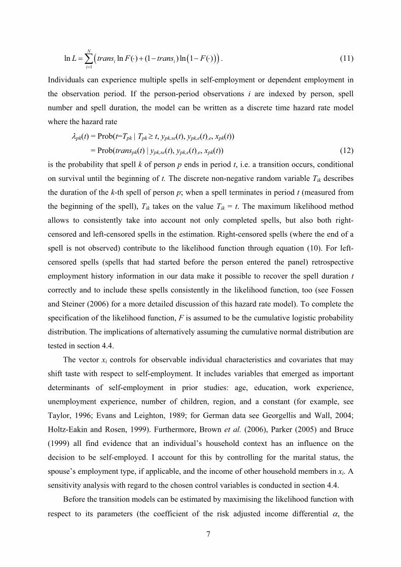
((1

ln ln ( ) (1 ) ln 1 ( )=

= ⋅ + − −∑N

i ii

L trans F trans F ))⋅ . (11)

Individuals can experience multiple spells in self-employment or dependent employment in

the observation period. If the person-period observations i are indexed by person, spell

number and spell duration, the model can be written as a discrete time hazard rate model

where the hazard rate

λpk(t) = Prob(t=Tpk | Tpk ≥ t, ypk,se(t), ypk,e(t),e, xpk(t))

= Prob(transpk(t) | ypk,se(t), ypk,e(t),e, xpk(t)) (12)

is the probability that spell k of person p ends in period t, i.e. a transition occurs, conditional

on survival until the beginning of t. The discrete non-negative random variable Tik describes

the duration of the k-th spell of person p; when a spell terminates in period t (measured from

the beginning of the spell), Tik takes on the value Tik = t. The maximum likelihood method

allows to consistently take into account not only completed spells, but also both right-

censored and left-censored spells in the estimation. Right-censored spells (where the end of a

spell is not observed) contribute to the likelihood function through equation (10). For left-

censored spells (spells that had started before the person entered the panel) retrospective

employment history information in our data make it possible to recover the spell duration t

correctly and to include these spells consistently in the likelihood function, too (see Fossen

and Steiner (2006) for a more detailed discussion of this hazard rate model). To complete the

specification of the likelihood function, F is assumed to be the cumulative logistic probability

distribution. The implications of alternatively assuming the cumulative normal distribution are

tested in section 4.4.

The vector xi controls for observable individual characteristics and covariates that may

shift taste with respect to self-employment. It includes variables that emerged as important

determinants of self-employment in prior studies: age, education, work experience,

unemployment experience, number of children, region, and a constant (for example, see

Taylor, 1996; Evans and Leighton, 1989; for German data see Georgellis and Wall, 2004;

Holtz-Eakin and Rosen, 1999). Furthermore, Brown et al. (2006), Parker (2005) and Bruce

(1999) all find evidence that an individual’s household context has an influence on the

decision to be self-employed. I account for this by controlling for the marital status, the

spouse’s employment type, if applicable, and the income of other household members in xi. A

sensitivity analysis with regard to the chosen control variables is conducted in section 4.4.

Before the transition models can be estimated by maximising the likelihood function with

respect to its parameters (the coefficient of the risk adjusted income differential α, the

7

coefficient of relative risk aversion ρ, the parameters of the baseline hazard δ1, δ2 and δ3

describing the duration dependence, and the parameter vector of the characteristics

influencing taste, β1), the expected value of income µy and its variance σy2 in the two

alternative employment states are required for each individual in each period, as these

statistics enter the likelihood function through V. The strategy for estimating µy and σy2 is

described in sections 3.3 and 3.5, after the data basis for this analysis is shortly described in

the next section.

3.2 Data

This analysis is based on the German Socio-Economic Panel (SOEP) provided by the German

Institute of Economic Research (DIW Berlin). The SOEP is a representative yearly panel

survey covering detailed information about the socio-economic situation of about 22,000

individuals living in 12,000 households in Germany. I use all 22 waves currently available

which cover the years from 1984 to 2005. The SOEP Group (2000) gives a detailed

description of the data.

For the purpose of this analysis, the sample is restricted to individuals between 18 and 64

years of age and excludes farmers, civil servants, and those currently in education, vocational

training, or military service. The individuals excluded presumably have a limited occupational

choice set, or they have different determinants of earnings (e.g. subsidies in the case of

farmers) and of occupational choice that could distort our analysis. Family members working

for a self-employed relative are also excluded from the dataset because they are not

entrepreneurs in the sense of running their own business. After removing observations with

missing values for any of the relevant variables, 117 321 person-year observations are left for

the analysis. Table A 1 in the appendix shows how these observations are distributed over the

possible employment states dependent employment, self-employment, and unemployment or

non-participation, further split by full-time and part-time work (full-time is defined as a

minimum of 35 hours per week) and gender. Working individuals are classified as self-

employed or dependently employed based on whether they report self-employment or

dependent employment as their primary activity. A transition can be identified in the data

when a person is observed in different employment states in two consecutive years t and t+1.

This paper focuses on the choice between full-time dependent employment and full-time

self-employment, because the attention is on the comparison of earnings in the two alternative

employment states, not on the decision to work full-time or part-time or the decision to work

or not to work. Thus, as in Taylor (1996) and Rees and Shah (1986), the structural transition

8

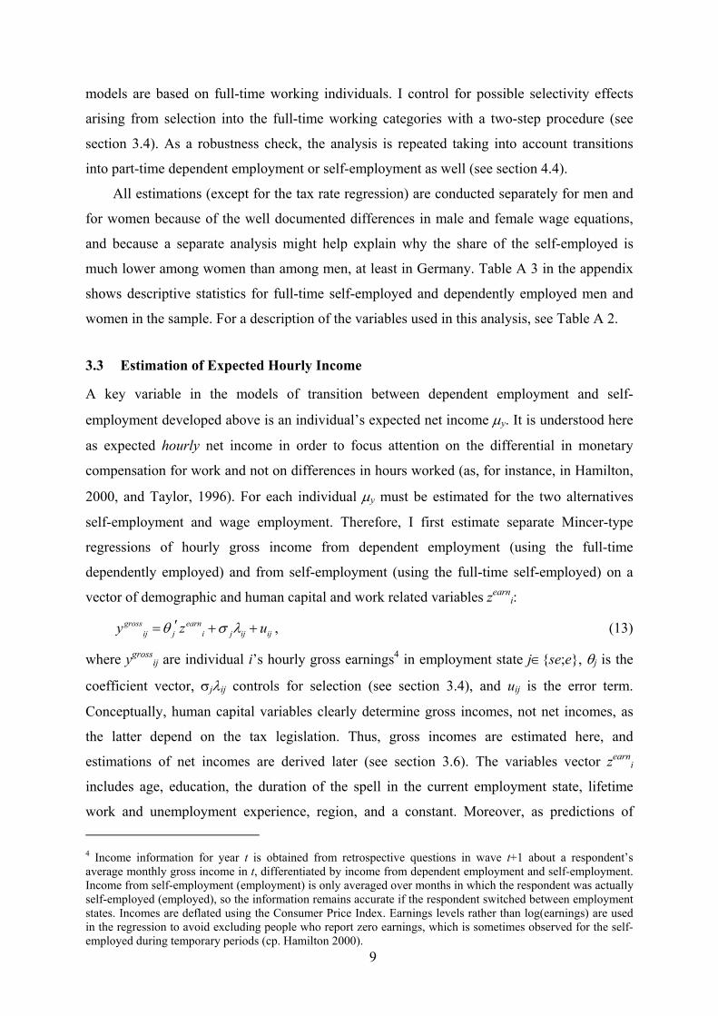
models are based on full-time working individuals. I control for possible selectivity effects

arising from selection into the full-time working categories with a two-step procedure (see

section 3.4). As a robustness check, the analysis is repeated taking into account transitions

into part-time dependent employment or self-employment as well (see section 4.4).

All estimations (except for the tax rate regression) are conducted separately for men and

for women because of the well documented differences in male and female wage equations,

and because a separate analysis might help explain why the share of the self-employed is

much lower among women than among men, at least in Germany. Table A 3 in the appendix

shows descriptive statistics for full-time self-employed and dependently employed men and

women in the sample. For a description of the variables used in this analysis, see T . able A 2

+ u

3.3 Estimation of Expected Hourly Income

A key variable in the models of transition between dependent employment and self-

employment developed above is an individual’s expected net income µy. It is understood here

as expected hourly net income in order to focus attention on the differential in monetary

compensation for work and not on differences in hours worked (as, for instance, in Hamilton,

2000, and Taylor, 1996). For each individual µy must be estimated for the two alternatives

self-employment and wage employment. Therefore, I first estimate separate Mincer-type

regressions of hourly gross income from dependent employment (using the full-time

dependently employed) and from self-employment (using the full-time self-employed) on a

vector of demographic and human capital and work related variables zearni:

θ σ λ′= +gross earnij j i j ij ijy z , (13)

where ygrossij are individual i’s hourly gross earnings4 in employment state j∈{se;e}, θj is the

coefficient vector, σjλij controls for selection (see section 3.4), and uij is the error term.

Conceptually, human capital variables clearly determine gross incomes, not net incomes, as

the latter depend on the tax legislation. Thus, gross incomes are estimated here, and

estimations of net incomes are derived later (see section 3.6). The variables vector zearni

includes age, education, the duration of the spell in the current employment state, lifetime

work and unemployment experience, region, and a constant. Moreover, as predictions of

9

4 Income information for year t is obtained from retrospective questions in wave t+1 about a respondent’s average monthly gross income in t, differentiated by income from dependent employment and self-employment. Income from self-employment (employment) is only averaged over months in which the respondent was actually self-employed (employed), so the information remains accurate if the respondent switched between employment states. Incomes are deflated using the Consumer Price Index. Earnings levels rather than log(earnings) are used in the regression to avoid excluding people who report zero earnings, which is sometimes observed for the self-employed during temporary periods (cp. Hamilton 2000).

income enter the structural transition models, for identification some variables should be

included in the earnings, but not in the transition equations. I follow Fraser and Greene

(2006), Taylor (1996) and Rees and Shah (1986) by including industry dummies, which are

well proven determinants of earnings, in zearni only.5

The estimated income models are then used to obtain individual predictions for gross

earnings in the two alternative states self-employment and dependent employment, one of

which is counter-factual, for every individual and period in the sample of the full-time

working population. If there are unobservable factors that both influence selection into full-

time self-employment or full-time dependent employment and income, it is necessary to

control for selection.

3.4 Selection

A two-step procedure is applied to control for selection effects in the earnings regressions

(13) (and also in the estimation of earnings variance (18) as will be described in the next

section). The earnings regressions are the 2nd step after the estimation of a 1st step equation of

selection into the 5 possible employment states spread out in Table A 1: full-time and part-

time self-employment, full-time and part-time dependent employment and

unemployment/inactivity. The probability of being observed in each of these 5 employment

states j is estimated by a reduced form multinomial logit:

( ) 5

1

exp( )Prob( )

exp( )

γγ

γ=

′′= = =

′∑j i

i i j i

k ik

zJ j z F z

z, (14)

where γj are the coefficient vectors6 and zi is the vector of regressors. This vector consist of

the variables zearni used in the earnings regression (13) (excluding spell duration), and for

identification, it additionally includes variables indicating a self-employed father7, the number

of children, and the marital status.8 After estimation of (14) an individual sample selection

5 Additionally dummy variables for German nationality and physical handicap are added to the earnings equations, as these variables turn out to be important for the prediction of earnings. Year dummies are also included to account for the business cycle. 6 γj is normalised to 0 for the base category j=”unemployment/inactivity” 7 Having a self-employed father is used as an exclusion restriction as this characteristic is likely to have an impact on the probability of being self-employed (e.g. Dunn and Holtz-Eakin 2000), e.g. through an inherited business, but is not expected to have an influence on earnings after controlling for other relevant factors (cp. Taylor 1996). In Germany, self-employed mothers were rare in the generation of most respondents’ parents, so only self-employed fathers are used.

10

8 The number of children and marital status are well known to influence the decision to participate in the labour market and the choice between part-time and full-time work, especially for women (e.g. Mroz 1987), but are not expected to influence gross earnings (cp. Rees and Shah, 1986).

term λij (similar to the “inverse Mill’s ratio”) is calculated for the two states of interest

j∈{se;e} (full-time self-employment and dependent employment):

( )( )( )

1 γλ φ

γ

− ′Φ= ′

j i

ij

j i

F z

F z

, (15)

where φ and Φ−1 are the standard normal density function and the inverse of the cumulative

standard normal density function. Then the term λij enters the earnings equation (13) for

earnings in employment state j∈{se;e}, which allows to estimate its coefficients σj. For the

subsequent prediction of an individual’s earnings in each of the two employment states, σjλij

enters the prediction equation if individual i is actually observed in that state, and in the

counter-factual case, σjλij,cf enters the equation with

( )( )( )

1

,1

γλ φ

γ

− ′Φ= − ′−

j i

ij cf

j i

F z

F z

. (16)

For a detailed description of the two-step procedure for polychotomous-choice models and

selectivity bias see Maddala (1983).

3.5 Estimation of Earnings Variance

Along with an individual’s expected income µy, the first moment of random earnings, the

individual variance of earnings σy2, i.e. the second moment, is also required to estimate the

transition models between dependent employment and self-employment. The literature on the

earnings differential has mostly analysed the first moment only, and if the second moment is

taken into account, as in Pfeiffer and Pohlmeier (1992) and in Rosen and Willen (2002), the

variance is usually modelled as a population parameter and not estimated on an individual

basis, which implies the assumption that income is homoscedastic. This assumption is relaxed

here, allowing the variance of earnings to differ not only between self-employment and

dependent employment, but also with individual characteristics and covariates.9 The point

made in this paper is that individuals do not only worry about the first, but also the second

moment of their individual probability distribution of income in the two alternative

employment states when they consider a transition.

As the error term in the earnings equation (13) uij has an expected value of 0, the

variance of gross random earnings conditional on the explanatory variables is

119 Therefore, heteroscedasticity robust (White) standard errors are reported in the earnings regression (13).

2 ( ) (σ = =gross grossy ijVar y E u 2 )ij

+ e

. (17)

Thus, the squared residuals from the earnings regression can be used to specify a flexible

heteroscedasticity function and estimate σgrossy2. The natural logarithm of the squared

residuals are regressed on the explanatory variables of the earnings model zearni and the

selection term λij from (15) to control for selection, separately for the two employment states

j∈{se;e}:

2ˆln( ) π σ λ′= +earn varij j i j ij iju z , (18)

where eij is the error term. Taking the logarithm of the squared residuals is the common

approach to ensure that predicted values for the variance are strictly positive.10 For the

prediction of the variance in the counter-factual employment state, λij is replaced by λij,cf from

(16) as in the earnings regression. This procedure yields individual predictions of the variance

of gross earnings, which is the basis for the calculation of the variance of net earnings, as will

be described in the next section.

3.6 Estimation of the Tax Function

As individual utility depends on net (after-tax) income, the relevant variables in the structural

transition models are the expected value and the variance of net income. To derive net income

from gross income, the German progressive income tax schedule must be approximated. As

the SOEP provides information about both a respondent’s gross and net income,11 individual

and period specific average tax rates τi, can be calculated:

τ −= i

ii

grossinc netincgrossinc

i

iv

, (19)

where grossinci and netinci are gross and net income per year. These tax rates τi, are regressed

on a vector ztaxi of variables relevant for the tax code:

τ κ ′= +taxi iz , (20)

where κ is the coefficient vector and vi is the error term capturing specifics of the tax

legislation which cannot be taken into account in this approximation.12 The vector ztaxi

includes polynomials of the first, second and third degree of gross yearly income to model the

10 To obtain consistent predictions for the squared residuals, the predicted values from the log model must be exponentiated and multiplied with the expected value of exp(eij). A consistent estimator for the expected value of exp(eij) is obtained from a regression of the squared residuals on the exponentiated predicted values from the log model through the origin. This procedure does not require normality of eij (see Wooldridge 2003). 11 Respondents are asked to state their gross and net income in the week before the interview.

12

12 All working respondents, no matter if full-time or part-time, provide information that is used to estimate this tax function.

non-linear nature of the tax function, a “married” dummy, additionally interacted with a

“female” dummy (to account for the effect of income splitting), the number of children, a

“disabled” dummy, and a “self-employed” dummy (to allow for differential tax treatment).

After this tax function is estimated, it can be used to predict average tax rates dependent on

the predicted gross incomes in both the true and the counter-factual employment state and

individual characteristics.13 This allows deriving the expected value and variance of net

incomes in both alternatives.

3.7 Calculation of Annuities

In the model developed above, agents considering a transition between the two employment

states dependent employment and self-employment compare the expected value µy and the

variance σy2 of net income in the two alternatives. Rational agents will not only take into

account next year’s returns when they consider a decision as important as starting or giving up

a self-employed venture, they will rather take into account the future curves of expected

income and income variance over the remaining years of their economic activity; the horizon

is assumed to be reached at 65 years (the retirement age in Germany). Thus, equations (13),

(18) and (20) are used to predict the expected net income and net income variance for each

individual in each of the two alternative employment states for all years until the individual

reaches the age of 65 by adjusting the duration in the respective employment state within the

explanatory variables. Then the capital value method is applied to calculate an annuity of

expected income:

( )( )

,

1

11

µ=

−=

−∑

i i

i

netn nij k

y knk

yq qqq

, (21)

where q is the real interest rate plus one14, and ni is the number of remaining years of

economic activity for individual i. The difference between net income derived from actual

gross income and net income derived from predicted net income in an individual’s actual

employment state ji in the year of observation is added to ynetij,k for j=ji, as this residual

contains additional information about an individual’s productivity in state ji. An annuity of

income variance is calculated analogously. These annuities finally enter the utility function

and thus the structural transition model (9).

13 Predicted ygross

ij are hourly incomes, whereas the tax function requires yearly income. For the conversion, the average number of hours worked in the sample of full-time working people is used.

1314 The real interest rate is assumed to be 5%. The sensitivity with respect to q is tested in section 4.4.

4 Empirical Results

4.1 Expected Value and Variance of Earnings

The reduced form multinomial logit equation of selection into the different employment states

(14) is estimated first. reports the estimated marginal effects of the variables on the

probabilities of the outcomes “full-time self-employment” and “full-time dependent

employment” for men and women.15 The significant marginal effects of fatherse indicate that

the probability of being full-time self-employed is 7.2 percentage points higher for men with a

self-employed father and 0.8 %-points for women. The higher probability confirms results

found in the literature (e.g. Dunn and Holtz-Eakin 2000; Taylor 1996). A child significantly

reduces the probability of being full-time dependently employed (21.9 %-points for women,

but only 1.8 %-points for men); the probability of being full-time self-employed is not

affected as much, it decreases for women whereas for men it even increases. Married men and

women have a lower probability of being full-time self-employed, whereas the effect for

dependent employment differs strongly between genders: Married women have an 18.8 %-

points lower probability of working full-time in dependent-employment, whereas men have a

13.8 %-points higher probability.

Table 1

INSERT TABLE 1 ABOUT HERE

Now the selectivity terms λij can be calculated using (15), and the 2nd step earnings equation

(13) can be estimated. The results from the earnings regressions are shown in .

Unemployment experience has a significant negative effect on earnings in dependent

employment and even more so in self-employment for both men and women. A university

degree strongly increases earnings for men, especially in self-employment. For women, the

positive effect is smaller in both employment states, and it is insignificant in self-employment.

The duration of the spell in the current employment state has a positive and significant

influence on earnings for self-employed and dependently employed men and for dependently

employed women (the income curves over time will be discussed in detail below). The

coefficient of the selectivity term λ is negative in all models, which indicates that the error

terms in the selection equation (14) and the earnings equation (13) are negatively correlated.

It is significant in the models of dependent employment only. Insignificant and sometimes

Table 2

14

15 The multinomial logit coefficients and the marginal effects for the outcome categories “part-time self-employment” and “part-time dependent employment” are available upon request.

negative selection terms in regressions of earnings from self-employment are often reported in

the literature (Brock and Evans 1986; Rees and Shah 1986; Evans and Leighton 1989; Dolton

and Makepeace 1990; and Borjas and Bronars 1989), suggesting that there is no significant

selection on unobservables; Taylor (1996), in contrast, reports positive and significant

selection effects.

INSERT TABLE 2 ABOUT HERE

Table 3 shows the estimation results of the earnings variance equation (18). For both

employment states and genders, the explanatory variables are jointly significant at

conventional significance levels, which confirms the hypothesis that earnings are

heteroscedastic (Breusch-Pagan test). This result shows that the variance of earnings not only

differs between dependent employment and self-employment, but also between individuals,

dependent on their characteristics and covariates. The coefficient of the selectivity term λ is

significant and positive in dependent employment, which indicates a positive correlation

between the error terms in the selection and the variance equations, and insignificant in self-

employment, like in the earnings regression.

INSERT TABLE 3 ABOUT HERE

Using the estimated earnings and earnings variance equations, the individual expected value

and variance of gross earnings in both dependent employment and self-employment can be

predicted. Before net earnings and the corresponding variance can be calculated, which are

needed for the structural transition models, the tax rate function (20) must be estimated. The

results of this estimation are given in Table 4. They show that the individual average tax rate

increases with gross income at diminishing rates, which reflects the progressive income tax

code in Germany. The coefficient of the self-employment dummy indicates that the average

tax rate of the self-employed is roughly 3.4 percentage points lower than the rate of their

dependently employed counterparts (see Fossen and Steiner (2006) for details on the

differential tax treatment of the self-employed).

INSERT TABLE 4 ABOUT HERE

15

As argued in section 3.7, not only the income in the next year, but in all future years of

economic activity are relevant for an individual considering a transition from dependent

employment to self-employment or vice versa. The predicted gross and net hourly income

curves over the duration of a spell in self-employment or dependent employment are plotted

for self-employed men and women in , and for dependently employed men and

women in (at mean values of the other explanatory variables). The net income curves

run below the corresponding gross income curves (the gap is the tax paid), and they are also

flatter, which reflects the progressive income taxation in Germany. In each diagram, the

income curves in the actual employment state and in the counter-factual employment state can

be directly compared. For reference, the scatter dots mark the mean gross hourly incomes of

people actually observed with the respective spell duration. The numbers at the dots indicate

how many observations with the respective spell duration are available in the sample.

Figure 1

Figure 1

Figure 2

shows that on average, self-employed men would initially earn higher hourly

gross income in dependent employment than in self-employment, but self-employment is

rewarded higher for them after about 15 years. Interestingly, net income is higher for them in

self-employment almost from the beginning on. This finding supports the hypothesis that

higher net earnings in self-employment induce the self-employed to choose this state. The

picture is similar for self-employed women, although women have to endure a considerable

period of slightly lower net earnings in self-employment before these exceed the counter-

factual wages from dependent employment.

INSERT FIGURE 1 ABOUT HERE

Dependently employed people would on average earn more if they were self-employed, both

in gross and in net terms, as Figure 2 shows. On its own, this finding could be interpreted as a

sign that earnings do not play a role in the choice of the employment state, or even of

irrational behaviour. The structural model developed in this paper offers a different

explanation, however: If employees do not only have a higher expected value of earnings in

the counter-factual state of self-employment, but also a higher variance of earnings, it may be

rational for them to choose dependent employment if they are risk-averse.

INSERT FIGURE 2 ABOUT HERE

16

Figure 3 and shed light on the variance of earnings in the two different employment

states. For better comparability, the variation coefficient (the standard deviation over the

mean) is plotted. Again, the curves are drawn by varying the spell duration and keeping the

explanatory variables fixed at their mean values, and the scatter dots indicate the actual mean

variation coefficients of earnings at the respective spell durations. The four diagrams show

that the variation coefficient is larger in self-employment for all groups, i.e. for actually self-

employed and dependently employed men and women, and both before and after tax. The

difference between the earnings variation in self-employment and dependent employment is

more pronounced for those actually dependently employed than for those actually self-

employed. Thus, switching to self-employment would require the dependently employed to

tolerate a much higher earnings risk, and risk aversion could explain why employees do not

switch to self-employment in spite of the higher expected value of earnings.

Figure 4

INSERT FIGURE 3 ABOUT HERE

INSERT FIGURE 4 ABOUT HERE

4.2 Estimation Results of the Transition Models

After the individual net earnings and net variance profiles over time (till the age of 65) are

summarised as annuities (see section 3.7), the structural models of transition probabilities

between the alternative employment states dependent employment and self-employment (9)

can be estimated. Table 5 shows the coefficients resulting from the likelihood maximisation

and the marginal effects in brackets where applicable. For each gender, the model of entry

into self-employment from dependent employment is shown in the left and the model of exit

from self-employment towards dependent employment in the right column. A positive sign of

a coefficient indicates that the corresponding variable increases the probability of a transition

to the alternative employment state, and the marginal effects show by how many percentage

points. A university degree, for example, increases the probability of entering self-

employment ceteris paribus by 0.26 percentage points for dependently employed men.

The estimates for the structural parameters ρ and α are given at the bottom of the table.

The coefficient of the risk adjusted differential between net income from self-employment

and from dependent employment α is significant in all models and positive in the models of

entry into self-employment and negative in the models of exit. The four models thus

17

consistently confirm the hypothesis that a higher risk adjusted net income in self-employment

in comparison to dependent employment induces people both to become and to remain self-

employed as the probability of entry is increased and the probability of exit is decreased.

The coefficient of constant relative risk aversion ρ is positive in all models, indicating

risk aversion, and significant except for self-employed women, for whom the null hypothesis

of risk neutrality cannot be rejected. The estimated degrees of risk aversion are low for self-

employed men, moderate for dependently employed men and high for dependently employed

women and lie in the range reported by the literature (e.g. Holt and Laury 2002; Binswanger

1980). Considering that far more women are dependently employed than self-employed, this

finding is also in line with Dohmen et al. (2005), who found that women are generally more

risk-averse than men. Self-employed men and women are clearly less risk-averse than

employees, which is consistent with the hypothesis that risk aversion deters people from

choosing self-employment. The finding that self-employed women may even be risk-neutral,

and thus less risk-averse than self-employed men, could be explained by the low share of the

self-employed among women in Germany, which may imply that only the least risk-averse

women choose self-employment.

INSERT TABLE 5 ABOUT HERE

Table 6 reports point elasticities of the transition probabilities with respect to the expected

value µy and the variance σy of net income in self-employment and in dependent employment.

They were calculated by evaluating the estimated structural transition model at the mean

values of the independent variables. All elasticities are significant except for the variance

elasticities of the probability of exit from self-employment for women. All elasticities have

the expected sign, indicating that higher net earnings in self-employment in comparison to

dependent employment attract people to this state, whereas higher relative variance deters

people from choosing this option. For example, the leftmost column shows that a 1 % rise in

the annuity of expected hourly net income in self-employment increases the probability of

entering self-employment by 1.4 % if the variance and the income in dependent employment

do not change. Similarly, a 1 % drop in net wages also raises the probability of entry into self-

employment by 1.15 % if the prospects in self-employment are unchanged. The elasticities do

not equal in absolute terms because of the different mean variance in the two employment

states. If the annuity of the net hourly income variance in self-employment increases by 1 %,

18

the probability of entry decreases by 0.16 %, and analogously, a 1 % rise in the variance of

wages increases the probability of entry by 0.05 %.

INSERT TABLE 6 ABOUT HERE

4.3 Illustration: Effect of the German Tax Reform 2000

To illustrate the results given in the previous section, in the following the estimated model is

used to simulate the ex-ante effects of the German Tax Reduction Act 2000

(Steuersenkungsgesetz 2000) on the transition rates between self-employment and dependent

employment. This reform significantly reduced income tax rates in several steps between

2001 and 2005. The top marginal income tax rate dropped from 51 % in 2000 to 42 % in 2005

and the lowest marginal tax rate from 22.9 % to 15 %. Haan and Steiner (2005) calculated the

relative change of net income due to the reform by income deciles using microsimulation

analysis. I draw on these results to calculate the net income individuals would have received

in 2000 if the full reform had already been in effect in that year. This allows comparing the

transition rates predicted by the model in the reform scenario with those in the baseline

scenario (using pre-reform net incomes in 2000); the difference in the transition rates is the

predicted response to the reform.16 For the 5337 individuals observed in 2000, the post-reform

expected values and variances of net incomes are calculated for both alternatives self-

employment and dependent employment and all future years, and lifetime annuities enter the

transition models in the same way as in the baseline scenario. reports the simulation

results. Due to the tax reform, for men the predicted exit rate out of self-employment drops by

almost 2 %-points, whereas the entry rate remains nearly unchanged. For women, the exit rate

virtually does not react to the tax reform, but the entry rate falls by 0.3 %-points. Altogether,

the tax reform promoted male self-employment and discouraged female self-employment.

This finding can be explained by the gender differences in tastes for risk and returns

expressed by ρ and α. On the one hand, the positive net income differential between self-

employment and dependent employment increases on average due to the tax reform, which

makes self-employment more attractive. On the other hand, the reform makes the tax schedule

less progressive, so the extent to which the high variance of earnings from self-employment is

Table 7

19

16 Income information for the year 2005 is not available in the SOEP yet, so the simulation cannot be performed after the full implementation of the reform.

levelled through taxation decreases. This discourages the more risk-averse dependently

employed women from entering self-employment.

INSERT TABLE 7 ABOUT HERE

4.4 Sensitivity Analysis

A number of assumptions were made in this paper in order to take the structural model

developed in section 2 to the data. This section assesses the sensitivity of the results with

respect to these assumptions. shows the structural parameters α and ρ and their robust

standard errors resulting from different specifications of the models. The baseline estimation

results are given in the first rows for reference. Overall, the estimated parameters are similar

in the different specifications and the basic results are thus found to be robust.17 When instead

of annuities over the individually remaining economically active years only the expected

value and variance of net income in the next year are used in the transition models, large

standard errors result and the structural coefficients in the transition models for men become

insignificant. As argued in section 3.7, it seems unlikely that agents only look at next year’s

income prospects when making a decision as important as a transition between dependent

employment and self-employment, and it would be irrational; thus, this special estimation

may not be very informative.

Table 8

INSERT TABLE 8 ABOUT HERE

5 Conclusion

The results of the analysis conducted in this paper show that not only the expected value, but

also the variance of an individual’s future after-tax income play a role in the choice between

self-employment and dependent employment. The probabilities of entry into self-employment

and also of exit are in general found to be significantly elastic with respect to both the first

and the second moments of net income in the two alternative employment states, and the

elasticities have the expected signs: Higher expected earnings in self-employment relative to

dependent employment attract people to become and to remain entrepreneurs, whereas higher

20

17 The probit coefficient of the risk adjusted income differential α can be multiplied by 1.6 for a rough comparison with the logit coefficient (Amemiya 1981).

variance discourages them from choosing this option. This can also be inferred from the

estimated coefficient of relative risk aversion which indicates that agents are moderately risk-

averse. Women’s higher risk aversion in comparison to men could be an explanation for the

low share of female entrepreneurs in Germany. The finding that entrepreneurial choice is at

least in part determined by a trade-off between returns and risks - in the sense of Kanbur

(1982) and Khilstrom and Laffont (1979) - is further supported by the empirical analysis of

incomes in dependent employment and self-employment. The estimated curves show that

controlling for selection, both the expected value and the variation coefficient of hourly net

earnings are on average higher in self-employment than in wage work in Germany, at least

after the initial years have passed.

The estimated structural models of self-employment entry and exit are relevant for policy

makers wishing to estimate the effect of changes to the progressive income tax code on self-

employment. An income tax reform generally influences both the mean of net income

(through the change in the individual average tax rate) and the variance of net income

(through the change in the progressiveness of the tax code). The effect of a reform on the

transition rates between dependent employment and self-employment can be simulated ex-

ante using the estimated structural transition models. This is especially interesting if the tax

reform is explicitly intended to promote the creation and survival of small businesses. The

model predicts that the German Tax Reduction Act of 2000 reduced the exit rates out of self-

employment for men and the entry rates for women, which in effect promoted male self-

employment and discouraged female self-employment.

21

References

Amemiya, Takeshi (1981), “Qualitative Response Models: A Survey,” Journal of Economic Literature 19 (4), pp. 481-536.

Binswanger, Hans P. (1980), “Attitudes toward Risk: Experimental Measurement in Rural India,“ American Journal of Agricultural Economics, Vol. 62, No. 3, pp. 395-407.

Borjas, George J. and Stephen G. Bronars (1989), “Consumer Discrimination and Self-Employment,” Journal of Political Economy, Vol. 97, pp. 581-605.

Brown, Sarah, Lisa Farrel and John G. Sessions (2006), “Self-Employment Matching – An Analysis of Dual Earner Couples and Working Households,” Small Business Economics 26, pp. 155-172.

Bruce, Donald (1999), “Do Husbands Matter? Married Women Entering Self-Employment,” Small Business Economics 13, pp. 317-329.

Bruce, Donald (2000), “Effects of the United States Tax System on Transitions into Self-Employment,” Labour Economics, Vol. 7, Issue 5, pp. 545-574.

Bruce, Donald (2002), “Taxes and Entrepreneurial Endurance: Evidence from the Self-Employed,” National Tax Journal, Vol. LV, No. 1.

Caliendo, Marco, Frank M. Fossen and Alexander S. Kritikos (2006), “Risk Attitudes of Nascent Entrepreneurs – New Evidence from an Experimentally-Validated Survey,” German Institute for Economic Research Research (DIW Berlin). DIW Discussion Paper No. 600.

Cramer, J.S., Joop Hartog, Nicole Jonker, and C. Mirjam Van Praag (2002), ”Low Risk Aversion Encourages the Choice for Entrepreneurship: An Empirical Test of a Truism,” Journal of Economic Behavior and Organization 48, pp. 29-36.

Cullen, Julie B. and Roger H. Gordon (2002), “Taxes and Entrepreneurial Activity: Theory and Evidence for the U.S.,” National Bureau of Economic Research. NBER Working Paper No. W9015.

Dunn, Thomas and Donald Holtz-Eakin (2000), “Financial capital, human capital, and the transition to self-employment: Evidence from Intergenerational Links,” Journal of Labour Economics 18, pp. 282-305.

Dohmen, Thomas, Armin Falk, David Huffman, Uwe Sunde, Jürgen Schupp and Gerd G. Wagner (2005), “Individual Risk Attitudes: New Evidence from a Large, Representative, Experimentally-Validated Survey,” German Institute for Economic Research Research (DIW Berlin). DIW Discussion Paper No. 511.

Dolton, Peter J. and Gerald H. Makepeace (1990), “Self-Employment Among Graduates,” Bulletin of Economic Research, Vol. 42 (1), pp. 35-53.

Domar, Evsey D. and Richard A. Musgrave (1944), “Proportional Income Taxation and Risk-Taking,” Quarterly Journal of Economics, 58, pp. 387-422.

22

Evans, David S. and Linda S. Leighton (1989), “Some Empirical Aspects of Entrepreneurship,” American Economic Review, Vol. 79, No. 3, pp. 519-535.

Fossen, Frank M. and Viktor Steiner (2006), “Income Taxes and Entrepreneurial Choice: Empirical Evidence from Germany,” German Institute for Economic Research (DIW Berlin). DIW Discussion Paper No. 582.

Fraser, Stuart and Francis J. Greene (2006), “The Effects of Experience on Entrepreneurial Optimism and Uncertainty,” Economica 73, pp. 169-192.

Gentry, William M. and R. Glenn Hubbard (2000), “Tax Policy and Entrepreneurial Entry,” American Economic Review, Vol. 90, pp. 283-287.

Georgellis, Yannis and Howard J. Wall (2002), “Entrepreneurship and the Policy Environment,” The Federal Reserve Bank of St. Louis. Working Paper 2002-019B.

Georgellis, Yannis and Howard J. Wall (2004), “Gender Differences in Self-Employment,” The Federal Reserve Bank of St. Louis. Working Paper 1999-008C.

Haan, Peter and Viktor Steiner (2005), “Distributional Effects of the German Tax Reform 2000 - A Behavioral Microsimulation Analysis,” Journal of Applied Social Science Studies 125, pp. 39-49.

Hamilton, Barton H. (2000), “Does Entrepreneurship Pay? An Empirical Analysis of the Returns to Self-Employment,” Journal of Political Economy, Vol. 108, No. 3, pp. 604-631.

Heaton, John and Deborah Lucas (2000), “Portfolio Choice and Asset Prices: The Importance of Entrepreneurial Risk,” The Journal of Finance LV, No. 3, pp. 1163-1198.

Holt, Charles A. and Susan K. Laury (2002), “Risk Aversion and Incentive Effects,” American Economic Review, Vol. 92, No. 5, pp. 1644-1655.

Holtz-Eakin, Douglas and Harvey S. Rosen (2005), “Cash Constraints and Business Start-Ups: Deutschmarks Versus Dollars,” Constributions to Economic Analysis & Policy, Vol. 4, No. 1.

Kanbur, Ravi S. M. (1982), “Entrepreneurial Risk Taking, Inequality, and Public Policy : An Application of Inequality Decomposition Analysis to the General Equilibirum of Progressive Taxation,“ Journal of Political Economy, Vol. 90, No. 1, pp. 1-21.

Kihlstrom, Richard E. and Jean-Jacques Laffont (1979), “A General Equilibrium Entrepreneurial Theory of Firm Formation Based on Risk Aversion,” The Journal of Political Economy, Vol. 87, No. 4, pp. 719-748.

Knight, Frank H. (1921), “Risk, Uncertainty and Profit” (Boston, MA: Hart, Schaffner & Marx; Houghton Mifflin Company).

Maddala, G.S. (1983), “Limited-Dependent and Qualitative Variables in Econometrics” (New York, NY: Cambridge University Press).

23

Moore, Kevin (2004), “The Effects of the 1986 and 1993 Tax Reforms on Self-Employment,” Board of Governors of the Federal Reserve System (U.S.). Finance and Economics Discussion Series Working Paper No. 2004-05.

Mroz, Thomas A. (1987), “The Sensitivity of an Empirical Model of Married Women’s Hours of Work to Economic and Statistical Assumptions,” Econometrica, Vol. 55, No. 4, pp. 765-799.

Parker, Simon C. (2003), “Does Tax Evasion Affect Occupational Choice?,” Oxford Bulletin of Economics and Statistics 63, pp. 379-394.

Parker, Simon C. (2005), “Entrepreneurship Among Married Couples in the United States – A Simultaneous Probit Approach,” Institute for the Study of Labor (IZA). IZA Discussion Paper No. 1712.

Pfeiffer, Friedhelm und Winfried Pohlmeier (1992), “Income, Uncertainty and the Probability of Self-Employment,” Recherches Economiques des Louvain 58 (3-4), pp. 265-281.

Pratt, John W. (1964), “Risk Aversion in the Small and in the Large,” Econometrica 32, pp. 122-136.

Rees, Hedley, and Anup Shah (1986), “An Empirical Analysis of Self-Employment in the U.K.,” Journal of Applied Econometrics 1, pp. 95-108.

Rosen, Harvey and Paul Willen (2002), “Risk, Return and Self-Employment,” mimeo, Princeton and Chicago Universities (2002), http://www.bos.frb.org/economic/econbios/willen/selfemp2.4pw.pdf.

Schuetze, Herbert J. (2000), “Taxes, Economic Conditions and Recent Trends in Male Self-employment: A Canada-U.S. Comparison,” Labour Economics 7 (5).

Schuetze, Herbert J., and Donald Bruce (2004), “Tax Policy and Entrepreneurship,“ Swedish Economic Policy Review 11, pp. 223-265.

SOEP Group (2000), “The German Socio-Economic Panel (GSOEP) after more than 15 years – Overview,” in: Elke Holst, Dr. Dean R. Lillard und Thomas A. DiPrete (ed.): Proceedings of the 2000 Fourth International Conference of German Socio-Economic Panel Study Users (GSOEP2000), Vierteljahrshefte zur Wirtschaftsforschung 70 (1), pp. 7-14.

Taylor, Mark P. (1996), “Earnings, Independence or Unemployment: Why Become Self-Employed?,” Oxford Bulletin of Economics and Statistics, Blackwell Publishing, Vol. 52, No. 2, pp. 253-265.

Taylor, Mark P. (1999), “Survival of The Fittest? An Analysis of Self-Employment Duration in Britain,” The Economic Journal 109, pp. C140-C155.

The Economist (2006), “Special Report: Germany's Export Champions,” The Economist Print Edition, Vol. 379, No. 8478, pp. 75-77.

Wooldridge, Jeffrey M. (2003), “Introductory Econometrics – A Modern Approach” (Mason, OH: Thomson South Western).

24

Tables

Table 1: Multinomial Logit Estimation of Employment State Probabilities Variable Marginal Effect on Outcome Probability

(Robust Standard Error) Men Women Full-Time Self-

Employed Full-Time Dep. Employed

Full-Time Self-Employed

Full-Time Dep. Employed

highschool 0.0057 -0.0303 0.0069 0.0258 (0.0026)* (0.0057)*** (0.0014)*** (0.0072)*** apprenticeship -0.0037 0.0864 -0.0027 0.0956 (0.0022) (0.0042)*** (0.0010)** (0.0056)*** highertechncol 0.0147 0.0546 0.0044 0.0927 (0.0028)*** (0.0040)*** (0.0013)*** (0.0072)*** university 0.0005 0.0761 0.0115 0.2503 (0.0027) (0.0043)*** (0.0019)*** (0.0094)*** age_bgn 0.0120 -0.0002 0.0014 -0.0062 (0.0010)*** (0.0016) (0.0004)*** (0.0022)** age_bgn_sq -0.0001 -0.0002 -0.0000 -0.0003 (0.0000)*** (0.0000)*** (0.0000)*** (0.0000)*** workexp_bgn -0.0001 0.0082 0.0017 0.0261 (0.0005) (0.0009)*** (0.0002)*** (0.0011)*** workexp_bgn_sq -0.0000 -0.0001 -0.0000 -0.0002 (0.0000)* (0.0000)*** (0.0000)*** (0.0000)*** unemexp -0.0140 -0.0576 -0.0054 -0.1013 (0.0013)*** (0.0025)*** (0.0009)*** (0.0035)*** unemexp_sq 0.0005 0.0034 0.0001 0.0058 (0.0001)*** (0.0003)*** (0.0002) (0.0004)*** german -0.0005 0.0551 0.0017 -0.0121 (0.0037) (0.0070)*** (0.0020) (0.0096) disabled -0.0208 -0.0655 -0.0098 0.0057 (0.0025)*** (0.0076)*** (0.0011)*** (0.0102) nchild 0.0046 -0.0175 -0.0034 -0.2187 (0.0008)*** (0.0017)*** (0.0006)*** (0.0031)*** married -0.0117 0.1383 -0.0055 -0.1883 (0.0022)*** (0.0047)*** (0.0012)*** (0.0057)*** fatherse 0.0721 -0.0960 0.0083 0.0270 (0.0048)*** (0.0071)*** (0.0019)*** (0.0081)*** Fed. state dummies YES YES YES YES Year dummies YES YES YES YES constant YES YES YES YES LR χ2 21190.336 33341.201 Pseudo R2 0.252 0.224 N 54157 63164 The table shows the marginal effects on the probabilities of the outcome categories “full-time self-employment” and “full-time dependent employment”. For dummy variables, the change in the probability caused by a discrete change from 0 to 1 are reported. The categories “part-time self-employment” and “part-time dependent employment” are not shown for brevity. The base category is “unemployment / inactivity”. Stars (* / ** / ***) indicate significance at the 5% / 1% / 0.1% level. Source: SOEP 1984-2005.

25

Table 2: Regression of Hourly Gross Earnings Variable Coefficient

(Robust Standard Error) Men Women Self-employed Dependently

employed Self-employed Dependently

employed duration 0.594 0.315 -0.305 0.358 (0.196)** (0.024)*** (0.378) (0.023)*** dur_sq -0.021 -0.005 0.039 -0.013 (0.014) (0.002)** (0.033) (0.002)*** dur_cu 0.000 0.000 -0.001 0.000 (0.000) (0.000) (0.001) (0.000)*** highschool -1.236 2.058 0.774 2.118 (0.938) (0.123)*** (1.170) (0.087)*** apprenticeship -1.715 0.166 -1.941 0.627 (1.075) (0.087) (1.209) (0.072)*** highertechncol -3.561 1.110 -2.020 0.726 (1.066)*** (0.107)*** (1.096) (0.108)*** university 6.652 3.888 1.303 2.634 (0.990)*** (0.147)*** (1.383) (0.106)*** age_bgn 0.367 0.179 0.216 0.095 (0.361) (0.041)*** (0.397) (0.036)** age_bgn_sq -0.004 0.001 -0.004 -0.001 (0.005) (0.001)* (0.005) (0.001) workexp_bgn 0.176 -0.111 -0.067 0.074 (0.120) (0.019)*** (0.283) (0.016)*** workexp_bgn_sq -0.001 -0.002 0.004 -0.002 (0.004) (0.001)*** (0.006) (0.001)** unemexp -1.819 -1.418 -2.993 -0.877 (0.484)*** (0.059)*** (0.887)*** (0.075)*** unemexp_sq 0.105 0.103 0.449 0.069 (0.053)* (0.008)*** (0.226)* (0.016)*** german -2.060 0.589 4.115 0.824 (1.185) (0.094)*** (1.812)* (0.091)*** disabled 0.095 -1.015 -2.987 -0.466 (1.195) (0.116)*** (2.765) (0.135)*** Fed. state dummies YES YES YES YES Year dummies YES YES YES YES Industry dummies YES YES YES YES λ -1.966 -0.642 -2.082 -0.407 (1.475) (0.230)** (3.789) (0.093)*** constant 7.217 5.523 -1.275 4.833 (9.361) (0.704)*** (15.583) (0.542)*** R2 0.186 0.370 0.285 0.313 N 3075 41365 991 22076 Stars (* / ** / ***) indicate significance at the 5% / 1% / 0.1% level. Source: Full-time self-employed and dependently employed individuals in the SOEP 1984-2005.

26

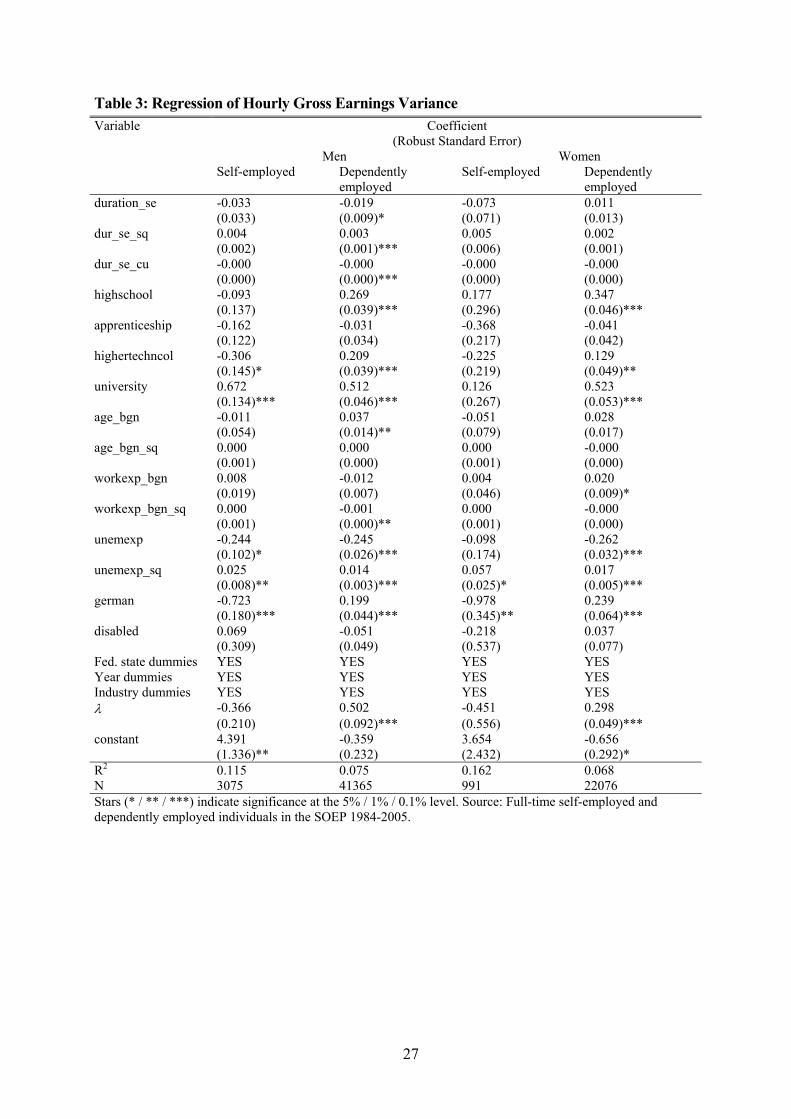
Table 3: Regression of Hourly Gross Earnings Variance Variable Coefficient

(Robust Standard Error) Men Women

Self-employed Dependently employed

Self-employed Dependently employed

duration_se -0.033 -0.019 -0.073 0.011 (0.033) (0.009)* (0.071) (0.013) dur_se_sq 0.004 0.003 0.005 0.002 (0.002) (0.001)*** (0.006) (0.001) dur_se_cu -0.000 -0.000 -0.000 -0.000 (0.000) (0.000)*** (0.000) (0.000) highschool -0.093 0.269 0.177 0.347 (0.137) (0.039)*** (0.296) (0.046)*** apprenticeship -0.162 -0.031 -0.368 -0.041 (0.122) (0.034) (0.217) (0.042) highertechncol -0.306 0.209 -0.225 0.129 (0.145)* (0.039)*** (0.219) (0.049)** university 0.672 0.512 0.126 0.523 (0.134)*** (0.046)*** (0.267) (0.053)*** age_bgn -0.011 0.037 -0.051 0.028 (0.054) (0.014)** (0.079) (0.017) age_bgn_sq 0.000 0.000 0.000 -0.000 (0.001) (0.000) (0.001) (0.000) workexp_bgn 0.008 -0.012 0.004 0.020 (0.019) (0.007) (0.046) (0.009)* workexp_bgn_sq 0.000 -0.001 0.000 -0.000 (0.001) (0.000)** (0.001) (0.000) unemexp -0.244 -0.245 -0.098 -0.262 (0.102)* (0.026)*** (0.174) (0.032)*** unemexp_sq 0.025 0.014 0.057 0.017 (0.008)** (0.003)*** (0.025)* (0.005)*** german -0.723 0.199 -0.978 0.239 (0.180)*** (0.044)*** (0.345)** (0.064)*** disabled 0.069 -0.051 -0.218 0.037 (0.309) (0.049) (0.537) (0.077) Fed. state dummies YES YES YES YES Year dummies YES YES YES YES Industry dummies YES YES YES YES λ -0.366 0.502 -0.451 0.298 (0.210) (0.092)*** (0.556) (0.049)*** constant 4.391 -0.359 3.654 -0.656 (1.336)** (0.232) (2.432) (0.292)* R2 0.115 0.075 0.162 0.068 N 3075 41365 991 22076 Stars (* / ** / ***) indicate significance at the 5% / 1% / 0.1% level. Source: Full-time self-employed and dependently employed individuals in the SOEP 1984-2005.

27

Table 4: Regression of Average Tax Rates Variable Coefficient (Robust Standard Error) grossinc_yr 0.052 (0.002)*** grossinc_yr_sq -0.002 (0.000)*** grossinc_yr_cu 1.45e-5 (0.000)*** self-employed -0.034 (0.002)*** married -0.046 (0.001)*** married x female 0.070 (0.001)*** nchild -0.017 (0.000)*** disabled -0.008 (0.002)*** year dummies YES constant 0.241 (0.003)*** mean avg. tax rate 0.328 R2 0.250 N 83101 Stars (***) indicate significance at the 0.1% level. Source: Self-employed and dependently employed individuals in the SOEP 1984-2005.

28

Table 5: Maximum Likelihood Estimation Results of Structural Transition Probabilities Variable / Structural Parameter

Coefficient / Estimated Value [Marginal Effect]

Men Women Dep. employment to

self-employment Self-employed to dep. employment

Dep. employment to self-employment

Self-employed to dep. employment

duration -0.2880*** -0.4066*** -0.3531*** 0.0987 [-0.0001] [-0.0015] [-0.0000] [-0.0022] dur_sq 0.0144*** 0.0190*** 0.0227** -0.0110 dur_cu -0.0003** -0.0002** -0.0004** 0.0002 highschool 0.0538 -0.3701 0.4431* 0.0367 [0.0001] [-0.0027] [0.0003] [0.0021] apprenticeship 0.6198*** 0.9552*** -0.1486 -0.2523 [0.0012] [0.0081] [-0.0001] [-0.0136] highertechncol 1.0088*** 0.7288** 0.2981 -0.5878 [0.0043] [0.0004] [0.0002] [-0.0089] university 0.6693*** -0.1735 0.0837 -1.0398*** [0.0026] [-0.0001] [0.0001] [-0.0157] age_bgn 0.0166 -0.1965*** 0.0384 -0.0930 [0.0000] [-0.0015] [0.0000] [-0.0052] age_bgn_sq -0.0010 0.0018** -0.0008 0.0005 workexp_bgn 0.0165 0.0007 0.0224 -0.0013 [0.0000] [0.0000] [0.0000] [-0.0001] unemexp 0.0544 -0.0877 0.1293 0.0173 [0.0001] [-0.0007] [0.0001] [0.0010] nchild 0.0664 0.0470 -0.0054 -0.3061* [0.0001] [0.0004] [-0.0000] [-0.0170] east 0.1622 0.1353 0.4067 0.7306* [0.0003] [0.0011] [0.0003] [0.0446] north -0.0900 -0.3605 -0.0967 -0.4851 [-0.0002] [-0.0025] [-0.0001] [-0.0231] south -0.3366** -0.1873 0.0756 -0.2832 [-0.0006] [-0.0014] [0.0000] [-0.0147] otherhhinc 0.0010 0.0019 -0.0149** 0.0014 [0.0000] [0.0000] [-0.0000] [0.0001] spouse_empl 0.2986* -0.0356 -0.1093 -0.3820 [0.0007] [-0.0003] [-0.0001] [-0.0196] spouse_selfempl 0.6352 0.1035 1.6111*** 0.9153*** [0.0018] [0.0008] [0.0023] [0.0677] spouse_notempl 0.1831 0.3229 0.0109 [0.0004] [0.0028] [0.0000] constant -4.5106*** 1.9661 -5.1964*** -0.5233 ρ 0.3901*** 0.1673*** 1.2878*** 0.0394 α 0.2625*** -0.2338*** 0.1378*** -0.3742*** Wald χ2 140.904 132.002 81.822 38.394 log likelihood -1579.163 -522.770 -611.151 -198.612 transitions (N) 388 232 133 78 transitions (rate) 0.009 0.075 0.006 0.083 N 41365 3075 22076 945 For self-employed women in our data, an unemployed/not working husband predicted a negative outcome (no transition) perfectly, so the 46 corresponding observations and the variable spouse_notempl were excluded from this estimation. Stars (* / ** / ***) indicate significance at the 10% / 5% / 1% level, based on heteroscedasticity robust standard errors. Source: Full-time self-employed and dependently employed individuals in the SOEP 1984-2005.

29

Table 6: Elasticities of Transition Probabilities with Respect to After-Tax µy and σy Elasticity Variable: Annuity of...

(Robust Standard Error) Men Women Dep. employment

to self-employmentSelf-employed to dep. employment

Dep. employment to self-employment

Self-employed to dep. employment

1.4359 -2.4640 1.4816 -2.7238 Hourly net earnings from self-employment (0.2501)*** (0.4600)*** (0.6664)** (0.7734)***

-1.1513 1.7619 -0.0848 2.6966 Hourly net earnings from dependent employment (0.2065)*** (0.4641)*** (0.0512)* (0.8283)***

-0.1584 0.5169 -0.6209 0.0526 Variance of hourly net earnings from self-employment (0.0127)*** (0.0386)*** (0.3287)* (0.0408)

0.0472 -0.0043 0.0041 -0.0030 Variance of hourly net earnings from dependent employment (0.0035)*** (0.0003)*** (0.0019)** (0.0023) The elasticities give the percentage change of the transition probabilities induced by a discrete one percent change in the annuities of expected value or variance of income from one of the two employment types, evaluated at the mean values of the explanatory variables in the sample. Stars (* / ** / ***) indicate significance at the 10% / 5% / 1% level. Source: Full-time self-employed and dependently employed individuals in the SOEP 1984-2005.

Table 7: Predicted Transition Rates in 2000 with and without Tax Reduction Act 2000 Predicted Transition Rate in % Men Women Dep. employment

to self-employmentSelf-employed to dep. employment

Dep. employment to self-employment

Self-employed to dep. employment

transition rate 2000 1.105 6.303 0.744 8.909 transition rate 2000 if full tax reform had been in effect already

1.110 4.340 0.440 8.923

difference (effect of tax reform) 0.005 -1.963 -0.304 0.015 N 3301 242 1722 72 All rates reported are significant at the 1% level. Source: Full-time self-employed and dependently employed individuals in the SOEP 1984-2005.

30

Table 8: Sensitivity Analysis of Structural Parameters in the Transition Models Structural Parameter

Estimated Value (Robust Standard Error)

Men Women Dep. employment to

self-employment Self-employed to dep. employment

Dep. employment to self-employment

Self-employed to dep. employment

Main estimation ρ 0.390 0.167 1.288 0.039 (0.051)*** (0.050)*** (0.229)*** (0.040) α 0.263 -0.234 0.138 -0.374 (0.022)*** (0.034)*** (0.025)*** (0.084)***

Exclusion of other household income ρ 0.390 0.168 1.287 0.039 (0.051)*** (0.050)*** (0.219)*** (0.040) α 0.262 -0.233 0.136 -0.374 (0.022)*** (0.034)*** (0.023)*** (0.084)***

Exclusion of number of children, other household income and spouse’s employment state ρ 0.394 0.167 1.213 0.042 (0.052)*** (0.050)*** (0.240)*** (0.040) α 0.261 -0.233 0.146 -0.367 (0.022)*** (0.034)*** (0.027)*** (0.082)***

Exclusion of unemployment experience ρ 0.390 0.168 1.302 0.040 (0.051)*** (0.050)*** (0.225)*** (0.039) α 0.262 -0.234 0.135 -0.374 (0.022)*** (0.034)*** (0.024)*** (0.083)***

Baseline hazard is a polynomial of forth degree ρ 0.390 0.166 1.284 0.039 (0.051)*** (0.050)*** (0.224)*** (0.040) α 0.262 -0.234 0.139 -0.374 (0.022)*** (0.034)*** (0.024)*** (0.084)***

Probit specification of the hazard rate ρ 0.480 1.225 0.081 (0.055)*** did not (0.192)*** (0.051) α 0.107 converge 0.068 -0.164 (0.009)*** (0.010)*** (0.034)***

Transitions to part-time self-employment / dependent empl. counted as positive outcome ρ 0.389 0.175 1.233 0.068 (0.048)*** (0.051)*** (0.199)*** (0.043) α 0.270 -0.236 0.152 -0.362 (0.021)*** (0.033)*** (0.024)*** (0.073)***

Real interest rate 8% (q=1.08) ρ 0.428 0.175 1.256 0.043 (0.061)*** (0.046)*** (0.221)*** (0.040) α 0.237 -0.221 0.136 -0.364 (0.022)*** (0.031)*** (0.024)*** (0.083)***

Real interest rate 2% (q=1.02) ρ 0.364 0.157 1.319 0.039 (0.045)*** (0.056)*** (0.246)*** (0.040) α 0.288 -0.248 0.140 -0.386 (0.022)*** (0.038)*** (0.026)*** (0.084)***

Consideration of next year’s expected income only instead of lifetime annuity ρ -0.489 -0.073 2.242 0.049 (0.701) (0.240) (0.630)*** (0.101) α -0.008 -0.037 0.116 -0.310 (0.022) (0.051) (0.135) (0.075)***

Combined estimation for men and women (including dummy variable for female) ρ 0.477 0.123 (0.050)*** (0.033)*** α 0.242 -0.256 (0.017)*** (0.031)*** Stars (* / ** / ***) indicate significance at the 10% / 5% / 1% level. Source: Full-time self-employed and dependently employed individuals in the SOEP 1984-2005.

31

Figures

Figure 1: Predicted Hourly Earnings of the Self-employed (Euros)

525395

306238

202

144

147128

107

9888

78

66

62

58

57

363237

27

2827

24

2417

21

17

1212

9

9

6

6

3

2

3

4

3 4

5

010

2030

0 10 20 30 40Spell Duration (years)

Gross Self-Empl. Earnings Gross WageNet Self-Empl. Earnings Net WageObserved Means of Gross Self-Empl. EarningsNumber of Observations Respective Tenure

Self-Employed Men

207

148

112

86

6553

5026

2527

21

262418

13

9

8 12

9

7

7

6

5

2

4

3

1

3

4

2

1

2

1

010

2030

0 10 20 30 40Spell Duration (years)

Gross Self-Empl. Earnings Gross WageNet Self-Empl. Earnings Net WageObserved Means of Gross Self-Empl. EarningsNumber of Observations Respective Tenure

Self-Employed Women

Figure 2: Predicted Hourly Earnings of Employees (Euros)

38763820

3427300927362309208518231651152114301309124511361060913797723643621579442435

418388367330292270258234214181179138

12110481

6048

010

2030

0 10 20 30 40Spell Duration (years)

Gross Self-Empl. Earnings Gross WageNet Self-Empl. Earnings Net WageObserved Means of Gross Self-Empl. EarningsNumber of Observations Respective Tenure

Dependently Employed Men

2703262222481873159713361157963845754663619555505454337297272246232216155148135138119

1191071008369

636251

50

503123

2525

010

2030

0 10 20 30 40Spell Duration (years)

Gross Self-Empl. Earnings Gross WageNet Self-Empl. Earnings Net WageObserved Means of Gross Self-Empl. EarningsNumber of Observations Respective Tenure

Dependently Employed Women

32

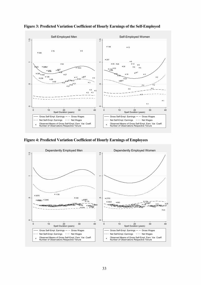
Figure 3: Predicted Variation Coefficient of Hourly Earnings of the Self-Employed

525

395

306

238

202

144147

128

10798

88

78

66

585736

32

37

27

28

27

24

24

1721

17

12

12

9

9

6 6

2

3

43

4

5

0.5

11.

5

0 10 20 30 40Spell Duration (years)

Gross Self-Empl. Earnings Gross WagesNet Self-Empl. Earnings Net WagesObserved Means of Gross Self-Empl. Earn. Var. Coeff.Number of Observations Respective Tenure

Self-Employed Men

207

148

11286

65

53

50

26

25

2721

26

24

18

13

9

812

9

7 7

6

5

2

4

3

1

4

2

2

10

.51

1.5

0 10 20 30 40Spell Duration (years)

Gross Self-Empl. Earnings Gross WagesNet Self-Empl. Earnings Net WagesObserved Means of Gross Self-Empl. Earn. Var. Coeff.Number of Observations Respective Tenure

Self-Employed Women

Figure 4: Predicted Variation Coefficient of Hourly Earnings of Employees

3876

38203427

300927362309

2085

182316511521143013091245

1136

1060913797723643621579442435418388367

330

292270258234

214181179

13812110481

6048

0.5

11.

5

0 10 20 30 40Spell Duration (years)

Gross Self-Empl. Earnings Gross WagesNet Self-Empl. Earnings Net WagesObserved Means of Gross Self-Empl. Earn. Var. Coeff.Number of Observations Respective Tenure

Dependently Employed Men

2703

2622

22481873159713361157

963

845754663619555505454337297272

246232216155148135

138

119119107

10083696362

51505031

23

2525

0.5

11.

5

0 10 20 30 40Spell Duration (years)

Gross Self-Empl. Earnings Gross WagesNet Self-Empl. Earnings Net WagesObserved Means of Gross Self-Empl. Earn. Var. Coeff.Number of Observations Respective Tenure

Dependently Employed Women

33

Appendix

Table A 1: Number of Person-Year Observations in the Different Employment States Employment State Category Men Women Unemployed/inactive 7976 26244 Full-time employed 41365 22076 Part-time employed 1460 13089 Full-time self-employed 3075 991 Part-time self-employed 281 764 Total 54157 63164 Source: SOEP 1984-2005.

Table A 2: Definition of Variables Variable Definition duration Duration of current spell (self-employment or employment). For left-censored spells, the

duration since the last job change is reported, which may be shorter than the overall duration in the current employment state if somebody switched jobs within one of these states before entering the panel

dur_sq, dur_cu Square and cube of duration variable highschool Dummy for individuals who have a high school degree ("Fachhochschulreife" or

"Abitur") apprenticeship Dummy for individuals who finished an apprenticeship ("Lehre") highertechnical Dummy for individuals who finished a higher technichal college or similar

("Berufsschule", "Schule Gesundheitswesen", "Fachschule", "Meister", "Beamtenausbildung", or "Sonstige Ausbildung")

university Dummy for individuals who have a university degree age_bgn Age at the beginning of the current spell in self-employment or dependent employment workexp_bgn Years of work experience at the beginning of the current spell unemexp Years of unemployement experience nchild Number of children under 17 in the household east Dummy for individuals who live in one of the 5 new eastern federal states or East Berlin north Dummy for individuals who live in one of the northern federal states (Schleswig Holstein,

Lower Saxony, Hamburg, or Bremen) south Dummy for individuals who live in one of the southern federal states (Baden-

Wuerttemberg or Bavaria) female Dummy for women otherhhinc Income of other individuals living in the same household per year (in € 1000) married Dummy for married individuals spouse_empl Dummy for married individuals whose spouse is dependently employed and living in the

same household spouse_selfempl Dummy for married individuals whose spouse is self-employed and living in the same

household spouse_notempl Dummy for married individuals whose spouse is unemployed or inactive and living in the

same household german Dummy for individuals with German nationality disabled Dummy for handicapped / physically challenged individuals fatherse Dummy for individuals whose father is/was self-employed grossinc_yr Gross income per year (€ 10 000) self-employed Dummy for self-employed individuals x_sq indicates the square and x_cu the cube of variable x. Dummy variables are equal to one if the condition holds and zero otherwise.

34

35

Table A 3: Descriptive Statistics Self-Employed

Men Women Variable Unit Mean Std Deviation Mean Std Deviationduration years 7.641 7.589 6.226 6.392highschool binary 0.349 0.306 apprenticeship binary 0.434 0.364 highertechncol binary 0.292 0.287 university binary 0.306 0.341 age_bgn years 36.838 9.204 38.532 9.567workexp_bgn years 13.581 9.680 13.911 9.352unemexp years 0.312 0.805 0.363 0.798nchild number 0.824 1.009 0.592 0.840east binary 0.228 0.386 north binary 0.155 0.127 south binary 0.264 0.210 otherhhinc (yr) € 1000 12.328 30.524 15.907 20.437married binary 0.724 0.719 spouse_empl binary 0.319 0.237 spouse_selfempl binary 0.074 0.154 spouse_notempl binary 0.127 0.046 german binary 0.945 0.964 disabled binary 0.035 0.015 fatherse binary 0.209 0.145 transitions (N) 232 78 transitions (rate) 0.075 0.079 N 3075 991

Dependently Employed Men Women Variable Unit Mean Std Deviation Mean Std Deviationduration years 9.915 8.559 8.110 7.611highschool binary 0.215 0.200 apprenticeship binary 0.565 0.529 highertechncol binary 0.205 0.210 university binary 0.182 0.202 age_bgn years 31.043 9.402 30.692 9.284workexp_bgn years 9.271 9.209 8.374 8.393unemexp years 0.390 0.965 0.371 0.866nchild number 0.779 0.992 0.387 0.696east binary 0.244 0.358 north binary 0.127 0.116 south binary 0.286 0.243 otherhhinc (yr) € 1000 12.682 20.808 16.209 20.368married binary 0.700 0.531 spouse_empl binary 0.283 0.264 spouse_selfempl binary 0.017 0.034 spouse_notempl binary 0.180 0.039 german binary 0.911 0.935 disabled binary 0.054 0.046 fatherse binary 0.066 0.082 transitions (N) 388 133 transitions (rate) 0.009 0.006 N 41365 22076 Standard deviations are given for continuous variables only. Source: Full-time self-employed and dependently employed individuals in the SOEP 1984-2005.