business analytics - 2. cluster analysis · 2020-06-04 · business analytics 1. k-means &...
TRANSCRIPT
Business Analytics
Business Analytics2. Cluster Analysis
Lars Schmidt-Thieme
Information Systems and Machine Learning Lab (ISMLL)University of Hildesheim, Germany
Lars Schmidt-Thieme, Information Systems and Machine Learning Lab (ISMLL), University of Hildesheim, Germany
1 / 36
Business Analytics
Outline
1. k-means & k-medoids
2. Hierarchical Cluster Analysis
3. Gaussian Mixture Models
4. Conclusion
Lars Schmidt-Thieme, Information Systems and Machine Learning Lab (ISMLL), University of Hildesheim, Germany
2 / 36
Business Analytics 1. k-means & k-medoids
Outline
1. k-means & k-medoids
2. Hierarchical Cluster Analysis
3. Gaussian Mixture Models
4. Conclusion
Lars Schmidt-Thieme, Information Systems and Machine Learning Lab (ISMLL), University of Hildesheim, Germany
2 / 36
Business Analytics 1. k-means & k-medoids
Partitions
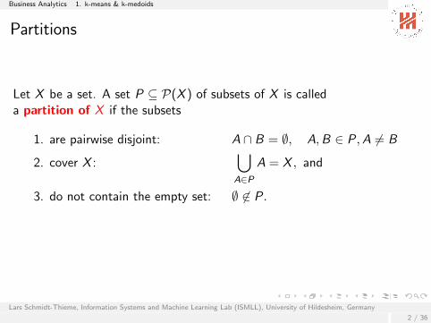
Let X be a set. A set P ⊆ P(X ) of subsets of X is calleda partition of X if the subsets
1. are pairwise disjoint: A ∩ B = ∅, A,B ∈ P,A 6= B
2. cover X :⋃A∈P
A = X , and
3. do not contain the empty set: ∅ 6∈ P.
Lars Schmidt-Thieme, Information Systems and Machine Learning Lab (ISMLL), University of Hildesheim, Germany
2 / 36

Business Analytics 1. k-means & k-medoids
Partitions
Let X := {x1, . . . , xN} be a finite set. A set P := {X1, . . . ,XK} of subsetsXk ⊆ X is called a partition of X if the subsets
1. are pairwise disjoint: Xk ∩ Xj = ∅, k , j ∈ {1, . . . ,K}, k 6= j
2. cover X :K⋃
k=1
Xk = X , and
3. do not contain the empty set: Xk 6= ∅, k ∈ {1, . . . ,K}.
The sets Xk are also called clusters, a partition P a clustering.K ∈ N is called number of clusters.
Part(X ) denotes the set of all partitions of X .
Lars Schmidt-Thieme, Information Systems and Machine Learning Lab (ISMLL), University of Hildesheim, Germany
2 / 36
Business Analytics 1. k-means & k-medoids
Partitions
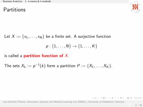
Let X := {x1, . . . , xN} be a finite set. A surjective function
p : {1, . . . ,N} → {1, . . . ,K}
is called a partition function of X .
The sets Xk := p−1(k) form a partition P := {X1, . . . ,XK}.
Lars Schmidt-Thieme, Information Systems and Machine Learning Lab (ISMLL), University of Hildesheim, Germany
2 / 36
Business Analytics 1. k-means & k-medoids
Partitions
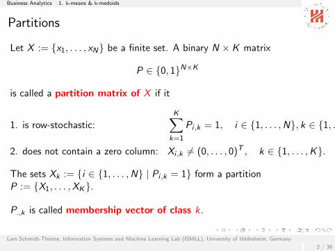
Let X := {x1, . . . , xN} be a finite set. A binary N × K matrix
P ∈ {0, 1}N×K
is called a partition matrix of X if it
1. is row-stochastic:K∑
k=1
Pi ,k = 1, i ∈ {1, . . . ,N}, k ∈ {1, . . . ,K}
2. does not contain a zero column: Xi ,k 6= (0, . . . , 0)T , k ∈ {1, . . . ,K}.
The sets Xk := {i ∈ {1, . . . ,N} | Pi ,k = 1} form a partitionP := {X1, . . . ,XK}.
P.,k is called membership vector of class k .
Lars Schmidt-Thieme, Information Systems and Machine Learning Lab (ISMLL), University of Hildesheim, Germany
2 / 36
Business Analytics 1. k-means & k-medoids
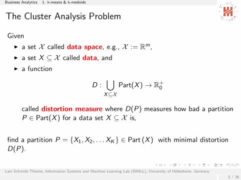
The Cluster Analysis Problem
Given
I a set X called data space, e.g., X := Rm,
I a set X ⊆ X called data, and
I a function
D :⋃
X⊆XPart(X )→ R+
0
called distortion measure where D(P) measures how bad a partitionP ∈ Part(X ) for a data set X ⊆ X is,
I a number K ∈ N of clusters,
find a partition P = {X1,X2, . . .XK} ∈ Part (X ) with minimal distortionD(P).
Lars Schmidt-Thieme, Information Systems and Machine Learning Lab (ISMLL), University of Hildesheim, Germany
3 / 36
Business Analytics 1. k-means & k-medoids
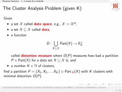
The Cluster Analysis Problem (given K)
Given
I a set X called data space, e.g., X := Rm,
I a set X ⊆ X called data,
I a function
D :⋃
X⊆XPart(X )→ R+
0
called distortion measure where D(P) measures how bad a partitionP ∈ Part(X ) for a data set X ⊆ X is, and
I a number K ∈ N of clusters,
find a partition P = {X1,X2, . . .XK} ∈ Part K (X ) with K clusters withminimal distortion D(P).
Lars Schmidt-Thieme, Information Systems and Machine Learning Lab (ISMLL), University of Hildesheim, Germany
3 / 36
Business Analytics 1. k-means & k-medoids
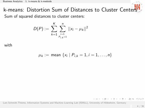
k-means: Distortion Sum of Distances to Cluster CentersSum of squared distances to cluster centers:
D(P) :=K∑
k=1
n∑i=1:
Pi.k=1
||xi − µk ||2
with
µk := mean {xi | Pi ,k = 1, i = 1, . . . , n}
Minimizing D over partitions with varying number of clusters leads tosingleton clustering with distortion 0; only the cluster analysis problemwith given K makes sense.
Minimizing D is not easy as reassigning a point to a different cluster alsoshifts the cluster centers.
Lars Schmidt-Thieme, Information Systems and Machine Learning Lab (ISMLL), University of Hildesheim, Germany
4 / 36
Business Analytics 1. k-means & k-medoids
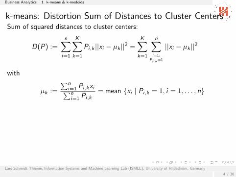
k-means: Distortion Sum of Distances to Cluster CentersSum of squared distances to cluster centers:
D(P) :=n∑
i=1
K∑k=1
Pi ,k ||xi − µk ||2 =K∑
k=1
n∑i=1:
Pi.k=1
||xi − µk ||2
with
µk :=
∑ni=1 Pi ,kxi∑ni=1 Pi ,k
= mean {xi | Pi ,k = 1, i = 1, . . . , n}
Minimizing D over partitions with varying number of clusters leads tosingleton clustering with distortion 0; only the cluster analysis problemwith given K makes sense.
Minimizing D is not easy as reassigning a point to a different cluster alsoshifts the cluster centers.
Lars Schmidt-Thieme, Information Systems and Machine Learning Lab (ISMLL), University of Hildesheim, Germany
4 / 36
Business Analytics 1. k-means & k-medoids
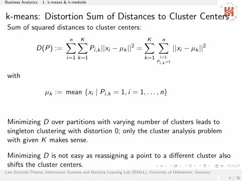
k-means: Distortion Sum of Distances to Cluster CentersSum of squared distances to cluster centers:
D(P) :=n∑
i=1
K∑k=1
Pi ,k ||xi − µk ||2 =K∑
k=1
n∑i=1:
Pi.k=1
||xi − µk ||2
with
µk := mean {xi | Pi ,k = 1, i = 1, . . . , n}
Minimizing D over partitions with varying number of clusters leads tosingleton clustering with distortion 0; only the cluster analysis problemwith given K makes sense.
Minimizing D is not easy as reassigning a point to a different cluster alsoshifts the cluster centers.
Lars Schmidt-Thieme, Information Systems and Machine Learning Lab (ISMLL), University of Hildesheim, Germany
4 / 36
Business Analytics 1. k-means & k-medoids
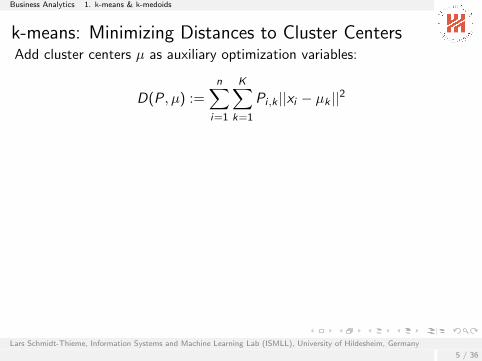
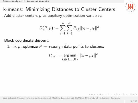
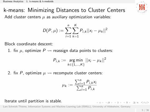
k-means: Minimizing Distances to Cluster CentersAdd cluster centers µ as auxiliary optimization variables:
D(P, µ) :=n∑
i=1
K∑k=1
Pi ,k ||xi − µk ||2
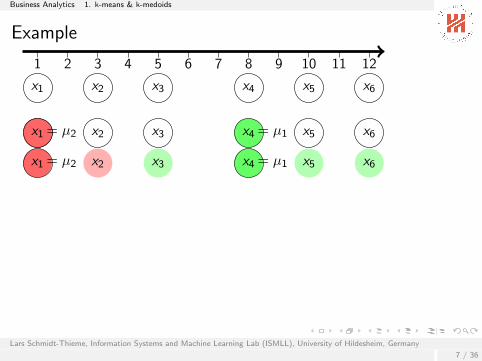
Block coordinate descent:
1. fix µ, optimize P reassign data points to clusters:
Pi ,k := arg mink∈{1,...,K}
||xi − µk ||2
2. fix P, optimize µ recompute cluster centers:
µk :=
∑ni=1 Pi ,kxi∑ni=1 Pi ,k
Iterate until partition is stable.
Lars Schmidt-Thieme, Information Systems and Machine Learning Lab (ISMLL), University of Hildesheim, Germany
5 / 36
Business Analytics 1. k-means & k-medoids
k-means: Minimizing Distances to Cluster CentersAdd cluster centers µ as auxiliary optimization variables:
D(P, µ) :=n∑
i=1
K∑k=1
Pi ,k ||xi − µk ||2
Block coordinate descent:
1. fix µ, optimize P reassign data points to clusters:
Pi ,k := arg mink∈{1,...,K}
||xi − µk ||2
2. fix P, optimize µ recompute cluster centers:
µk :=
∑ni=1 Pi ,kxi∑ni=1 Pi ,k
Iterate until partition is stable.Lars Schmidt-Thieme, Information Systems and Machine Learning Lab (ISMLL), University of Hildesheim, Germany
5 / 36
Business Analytics 1. k-means & k-medoids
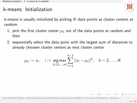
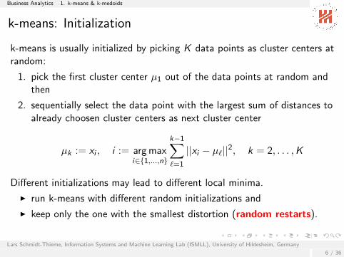
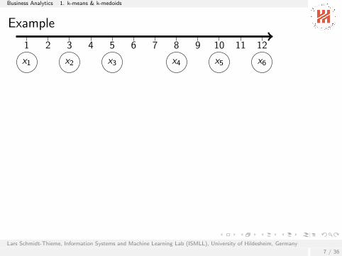
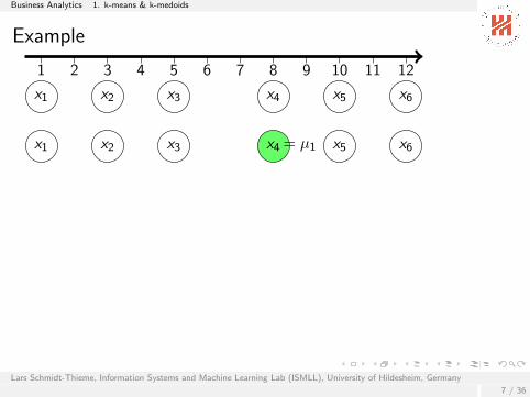
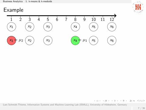
k-means: Initialization
k-means is usually initialized by picking K data points as cluster centers atrandom:
1. pick the first cluster center µ1 out of the data points at random andthen
2. sequentially select the data point with the largest sum of distances toalready choosen cluster centers as next cluster center
µk := xi , i := arg maxi∈{1,...,n}
k−1∑`=1
||xi − µ`||2, k = 2, . . . ,K
Different initializations may lead to different local minima.
I run k-means with different random initializations and
I keep only the one with the smallest distortion (random restarts).
Lars Schmidt-Thieme, Information Systems and Machine Learning Lab (ISMLL), University of Hildesheim, Germany
6 / 36
Business Analytics 1. k-means & k-medoids
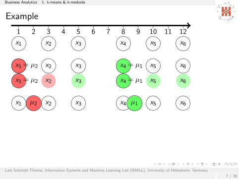
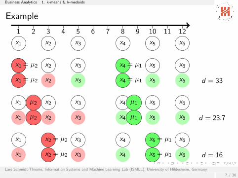
Example
1 2 3 4 5 6 7 8 9 10 11 12
x1 x2 x3 x4 x5 x6
x1 x2 x3 x4 = µ1 x5 x6
x1 = µ2 x2 x3 x4 = µ1 x5 x6
x1 µ2 x2 x3 x4 µ1 x5 x6
x1 µ2 x2 x3 x4 µ1 x5 x6
x1 x2 = µ2 x3 x4 x5 = µ1 x6
x1 x2 = µ2 x3 x4 x5 = µ1 x6
d = 33
d = 23.7
d = 16
Lars Schmidt-Thieme, Information Systems and Machine Learning Lab (ISMLL), University of Hildesheim, Germany
7 / 36
Business Analytics 1. k-means & k-medoids
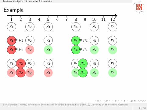
Example
1 2 3 4 5 6 7 8 9 10 11 12
x1 x2 x3 x4 x5 x6
x1 x2 x3 x4 = µ1 x5 x6x1 = µ2
x1 = µ2 x2 x3 x4 = µ1 x5 x6
x1 µ2 x2 x3 x4 µ1 x5 x6
x1 µ2 x2 x3 x4 µ1 x5 x6
x1 x2 = µ2 x3 x4 x5 = µ1 x6
x1 x2 = µ2 x3 x4 x5 = µ1 x6
d = 33
d = 23.7
d = 16
Lars Schmidt-Thieme, Information Systems and Machine Learning Lab (ISMLL), University of Hildesheim, Germany
7 / 36
Business Analytics 1. k-means & k-medoids
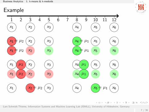
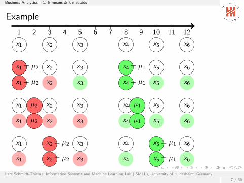
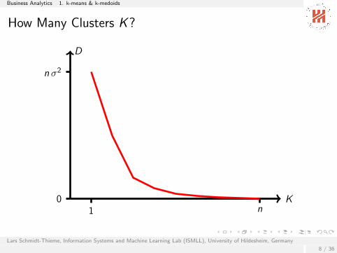
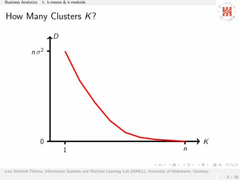
How Many Clusters K?
K
D
n σ2
01 n
Lars Schmidt-Thieme, Information Systems and Machine Learning Lab (ISMLL), University of Hildesheim, Germany
8 / 36
Business Analytics 1. k-means & k-medoids
How Many Clusters K?
K
D
n σ2
01 n
Lars Schmidt-Thieme, Information Systems and Machine Learning Lab (ISMLL), University of Hildesheim, Germany
8 / 36
Business Analytics 1. k-means & k-medoids
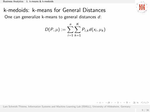
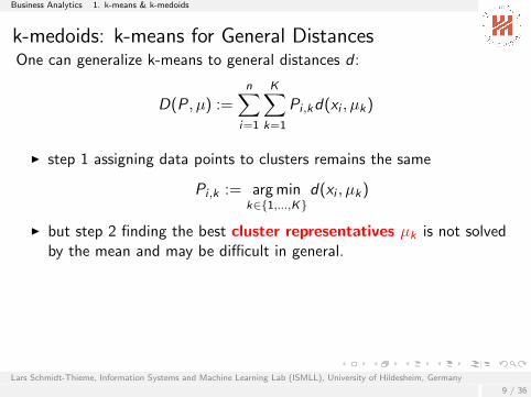
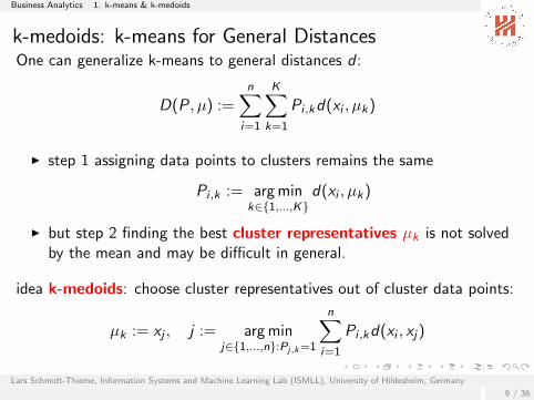
k-medoids: k-means for General DistancesOne can generalize k-means to general distances d :
D(P, µ) :=n∑
i=1
K∑k=1
Pi ,kd(xi , µk)
I step 1 assigning data points to clusters remains the same
Pi ,k := arg mink∈{1,...,K}
d(xi , µk)
I but step 2 finding the best cluster representatives µk is not solvedby the mean and may be difficult in general.
idea k-medoids: choose cluster representatives out of cluster data points:
µk := xj , j := arg minj∈{1,...,n}:Pj,k=1
n∑i=1
Pi ,kd(xi , xj)
Lars Schmidt-Thieme, Information Systems and Machine Learning Lab (ISMLL), University of Hildesheim, Germany
9 / 36
Business Analytics 1. k-means & k-medoids
k-medoids: k-means for General Distances
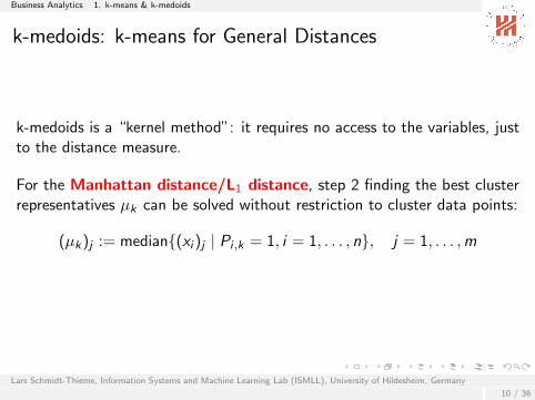
k-medoids is a “kernel method”: it requires no access to the variables, justto the distance measure.
For the Manhattan distance/L1 distance, step 2 finding the best clusterrepresentatives µk can be solved without restriction to cluster data points:
(µk)j := median{(xi )j | Pi ,k = 1, i = 1, . . . , n}, j = 1, . . . ,m
Lars Schmidt-Thieme, Information Systems and Machine Learning Lab (ISMLL), University of Hildesheim, Germany
10 / 36
Business Analytics 2. Hierarchical Cluster Analysis
Outline
1. k-means & k-medoids
2. Hierarchical Cluster Analysis
3. Gaussian Mixture Models
4. Conclusion
Lars Schmidt-Thieme, Information Systems and Machine Learning Lab (ISMLL), University of Hildesheim, Germany
11 / 36
Business Analytics 2. Hierarchical Cluster Analysis
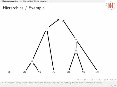
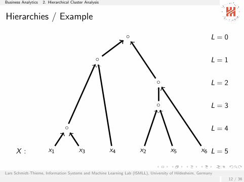
Hierarchies
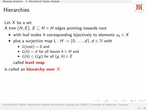
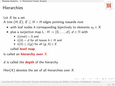
Let X be a set.A tree (H,E ), E ⊆ H × H edges pointing towards root
I with leaf nodes h corresponding bijectively to elements xh ∈ XI plus a surjective map L : H → {0, . . . , d}, d ∈ N with
I L(root) = 0 andI L(h) = d for all leaves h ∈ H andI L(h) ≤ L(g) for all (g , h) ∈ E
called level map
is called an hierarchy over X .
d is called the depth of the hierarchy.
Hier(X ) denotes the set of all hierarchies over X .
Lars Schmidt-Thieme, Information Systems and Machine Learning Lab (ISMLL), University of Hildesheim, Germany
11 / 36
Business Analytics 2. Hierarchical Cluster Analysis
Hierarchies
Let X be a set.A tree (H,E ), E ⊆ H × H edges pointing towards root
I with leaf nodes h corresponding bijectively to elements xh ∈ XI plus a surjective map L : H → {0, . . . , d}, d ∈ N with
I L(root) = 0 andI L(h) = d for all leaves h ∈ H andI L(h) ≤ L(g) for all (g , h) ∈ E
called level map
is called an hierarchy over X .
d is called the depth of the hierarchy.
Hier(X ) denotes the set of all hierarchies over X .
Lars Schmidt-Thieme, Information Systems and Machine Learning Lab (ISMLL), University of Hildesheim, Germany
11 / 36
Business Analytics 2. Hierarchical Cluster Analysis
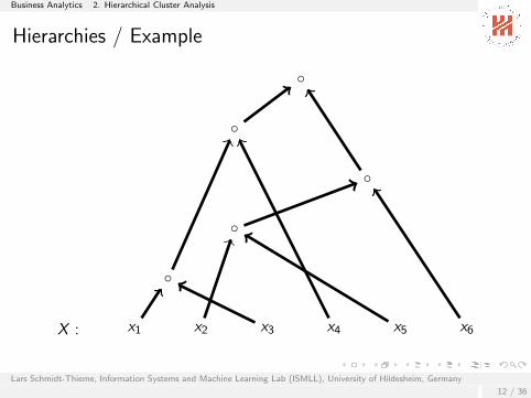
Hierarchies / Example
X : x1 x2 x3 x4 x5 x6
◦
◦
◦
◦
◦
Lars Schmidt-Thieme, Information Systems and Machine Learning Lab (ISMLL), University of Hildesheim, Germany
12 / 36
Business Analytics 2. Hierarchical Cluster Analysis
Hierarchies / Example
X : x1 x2 x3 x4 x5 x6
◦
◦
◦
◦
◦
Lars Schmidt-Thieme, Information Systems and Machine Learning Lab (ISMLL), University of Hildesheim, Germany
12 / 36
Business Analytics 2. Hierarchical Cluster Analysis
Hierarchies / Example
X : x1 x3 x4 x2 x5 x6
◦
◦
◦
◦
◦
L = 0
L = 1
L = 2
L = 3
L = 4
L = 5
Lars Schmidt-Thieme, Information Systems and Machine Learning Lab (ISMLL), University of Hildesheim, Germany
12 / 36
Business Analytics 2. Hierarchical Cluster Analysis
Hierarchies / Example
X : x1 x3 x4 x2 x5 x6
◦
◦
◦
◦
◦ L = 0
L = 1
L = 2
L = 3
L = 4
L = 5
Lars Schmidt-Thieme, Information Systems and Machine Learning Lab (ISMLL), University of Hildesheim, Germany
12 / 36
Business Analytics 2. Hierarchical Cluster Analysis
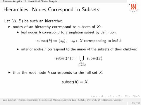
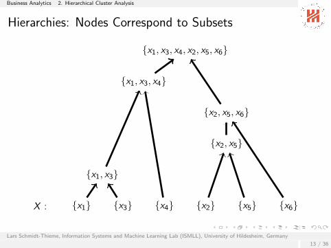
Hierarchies: Nodes Correspond to Subsets
Let (H,E ) be such an hierarchy:I nodes of an hierarchy correspond to subsets of X :
I leaf nodes h correspond to a singleton subset by definition.
subset(h) := {xh}, xh ∈ X corresponding to leaf h
I interior nodes h correspond to the union of the subsets of their children:
subset(h) :=⋃g∈H
(g,h)∈E
subset(g)
I thus the root node h corresponds to the full set X :
subset(h) = X
Lars Schmidt-Thieme, Information Systems and Machine Learning Lab (ISMLL), University of Hildesheim, Germany
13 / 36
Business Analytics 2. Hierarchical Cluster Analysis
Hierarchies: Nodes Correspond to Subsets
X : {x1} {x3} {x4} {x2} {x5} {x6}
{x1, x3}
{x2, x5}
{x2, x5, x6}
{x1, x3, x4}
{x1, x3, x4, x2, x5, x6}
Lars Schmidt-Thieme, Information Systems and Machine Learning Lab (ISMLL), University of Hildesheim, Germany
13 / 36
Business Analytics 2. Hierarchical Cluster Analysis
Hierarchies: Levels Correspond to Partitions
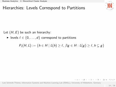
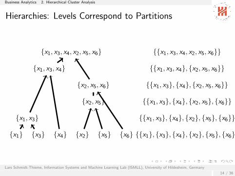
Let (H,E ) be such an hierarchy:
I levels ` ∈ {0, . . . , d} correspond to partitions
P`(H, L) := {h ∈ H | L(h) ≥ `, 6 ∃g ∈ H : L(g) ≥ `, h ( g}
Lars Schmidt-Thieme, Information Systems and Machine Learning Lab (ISMLL), University of Hildesheim, Germany
14 / 36
Business Analytics 2. Hierarchical Cluster Analysis
Hierarchies: Levels Correspond to Partitions
{x1} {x3} {x4} {x2} {x5} {x6}
{x1, x3}
{x2, x5}
{x2, x5, x6}
{x1, x3, x4}
{x1, x3, x4, x2, x5, x6} {{x1, x3, x4, x2, x5, x6}}
{{x1, x3, x4}, {x2, x5, x6}}
{{x1, x3}, {x4}, {x2, x5, x6}}
{{x1, x3}, {x4}, {x2, x5}, {x6}}
{{x1, x3}, {x4}, {x2}, {x5}, {x6}}
{{x1}, {x3}, {x4}, {x2}, {x5}, {x6}}
Lars Schmidt-Thieme, Information Systems and Machine Learning Lab (ISMLL), University of Hildesheim, Germany
14 / 36
Business Analytics 2. Hierarchical Cluster Analysis
The Hierarchical Cluster Analysis Problem
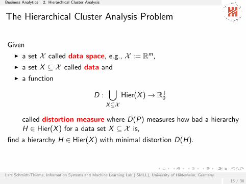
Given
I a set X called data space, e.g., X := Rm,
I a set X ⊆ X called data and
I a function
D :⋃
X⊆XHier(X )→ R+
0
called distortion measure where D(P) measures how bad a hierarchyH ∈ Hier(X ) for a data set X ⊆ X is,
find a hierarchy H ∈ Hier(X ) with minimal distortion D(H).
Lars Schmidt-Thieme, Information Systems and Machine Learning Lab (ISMLL), University of Hildesheim, Germany
15 / 36
Business Analytics 2. Hierarchical Cluster Analysis
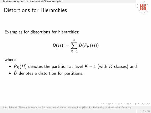
Distortions for Hierarchies
Examples for distortions for hierarchies:
D(H) :=n∑
K=1
D̃(PK (H))
where
I PK (H) denotes the partition at level K − 1 (with K classes) and
I D̃ denotes a distortion for partitions.
Lars Schmidt-Thieme, Information Systems and Machine Learning Lab (ISMLL), University of Hildesheim, Germany
16 / 36
Business Analytics 2. Hierarchical Cluster Analysis
Agglomerative and Divisive Hierarchical Clustering
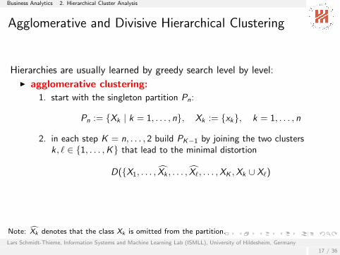
Hierarchies are usually learned by greedy search level by level:I agglomerative clustering:
1. start with the singleton partition Pn:
Pn := {Xk | k = 1, . . . , n}, Xk := {xk}, k = 1, . . . , n
2. in each step K = n, . . . , 2 build PK−1 by joining the two clustersk, ` ∈ {1, . . . ,K} that lead to the minimal distortion
D({X1, . . . , X̂k , . . . , X̂`, . . . ,XK ,Xk ∪ X`)
Lars Schmidt-Thieme, Information Systems and Machine Learning Lab (ISMLL), University of Hildesheim, Germany
17 / 36
Note: X̂k denotes that the class Xk is omitted from the partition.
Business Analytics 2. Hierarchical Cluster Analysis
Agglomerative and Divisive Hierarchical Clustering
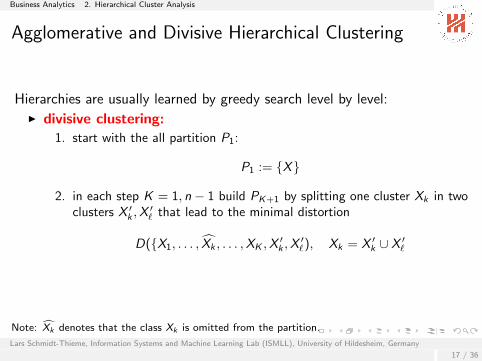
Hierarchies are usually learned by greedy search level by level:I divisive clustering:
1. start with the all partition P1:
P1 := {X}
2. in each step K = 1, n − 1 build PK+1 by splitting one cluster Xk in twoclusters X ′k ,X
′` that lead to the minimal distortion
D({X1, . . . , X̂k , . . . ,XK ,X′k ,X
′`), Xk = X ′k ∪ X ′`
Lars Schmidt-Thieme, Information Systems and Machine Learning Lab (ISMLL), University of Hildesheim, Germany
17 / 36
Note: X̂k denotes that the class Xk is omitted from the partition.
Business Analytics 2. Hierarchical Cluster Analysis
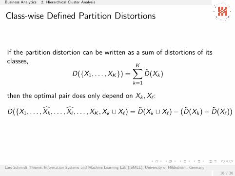
Class-wise Defined Partition Distortions
If the partition distortion can be written as a sum of distortions of itsclasses,
D({X1, . . . ,XK}) =K∑
k=1
D̃(Xk)
then the optimal pair does only depend on Xk ,X`:
D({X1, . . . , X̂k , . . . , X̂`, . . . ,XK ,Xk ∪ X`) = D̃(Xk ∪ X`)− (D̃(Xk) + D̃(X`))
Lars Schmidt-Thieme, Information Systems and Machine Learning Lab (ISMLL), University of Hildesheim, Germany
18 / 36
Business Analytics 2. Hierarchical Cluster Analysis
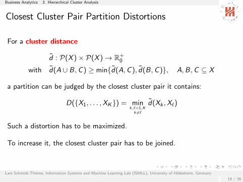
Closest Cluster Pair Partition Distortions
For a cluster distance
d̃ : P(X )× P(X )→ R+0
with d̃(A ∪ B,C ) ≥ min{d̃(A,C ), d̃(B,C )}, A,B,C ⊆ X
a partition can be judged by the closest cluster pair it contains:
D({X1, . . . ,XK}) = mink,`=1,K
k 6=`
d̃(Xk ,X`)
Such a distortion has to be maximized.
To increase it, the closest cluster pair has to be joined.
Lars Schmidt-Thieme, Information Systems and Machine Learning Lab (ISMLL), University of Hildesheim, Germany
19 / 36
Business Analytics 2. Hierarchical Cluster Analysis
Single Link Clustering
dsl(A,B) := minx∈A,y∈B
d(x , y), A,B ⊆ X
Lars Schmidt-Thieme, Information Systems and Machine Learning Lab (ISMLL), University of Hildesheim, Germany
20 / 36
Business Analytics 2. Hierarchical Cluster Analysis
Complete Link Clustering
dcl(A,B) := maxx∈A,y∈B
d(x , y), A,B ⊆ X
Lars Schmidt-Thieme, Information Systems and Machine Learning Lab (ISMLL), University of Hildesheim, Germany
21 / 36
Business Analytics 2. Hierarchical Cluster Analysis
Average Link Clustering
dal(A,B) :=1
|A||B|∑
x∈A,y∈Bd(x , y), A,B ⊆ X
Lars Schmidt-Thieme, Information Systems and Machine Learning Lab (ISMLL), University of Hildesheim, Germany
22 / 36
Business Analytics 2. Hierarchical Cluster Analysis
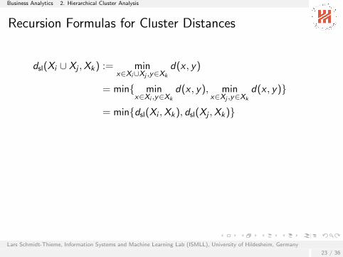
Recursion Formulas for Cluster Distances
dsl(Xi ∪ Xj ,Xk) := minx∈Xi∪Xj ,y∈Xk
d(x , y)
= min{ minx∈Xi ,y∈Xk
d(x , y), minx∈Xj ,y∈Xk
d(x , y)}
= min{dsl(Xi ,Xk), dsl(Xj ,Xk)}
dcl(Xi ∪ Xj ,Xk) = max{dcl(Xi ,Xk), dcl(Xj ,Xk)}
dal(Xi ∪ Xj ,Xk) =|Xi |
|Xi |+ |Xj |dal(Xi ,Xk) +
|Xj ||Xi |+ |Xj |
dal(Xj ,Xk)
agglomerative hierarchical clustering requires to compute thedistance matrix D ∈ Rn×n only once:
Di ,j := d(xi , xj), i , j = 1, . . . ,K
Lars Schmidt-Thieme, Information Systems and Machine Learning Lab (ISMLL), University of Hildesheim, Germany
23 / 36
Business Analytics 2. Hierarchical Cluster Analysis
Recursion Formulas for Cluster Distances
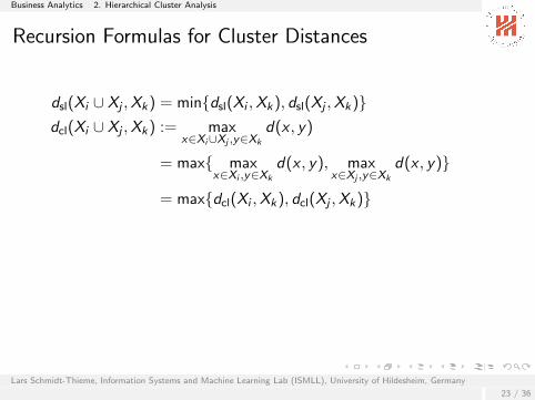
dsl(Xi ∪ Xj ,Xk) = min{dsl(Xi ,Xk), dsl(Xj ,Xk)}dcl(Xi ∪ Xj ,Xk) := max
x∈Xi∪Xj ,y∈Xk
d(x , y)
= max{ maxx∈Xi ,y∈Xk
d(x , y), maxx∈Xj ,y∈Xk
d(x , y)}
= max{dcl(Xi ,Xk), dcl(Xj ,Xk)}
dal(Xi ∪ Xj ,Xk) =|Xi |
|Xi |+ |Xj |dal(Xi ,Xk) +
|Xj ||Xi |+ |Xj |
dal(Xj ,Xk)
agglomerative hierarchical clustering requires to compute thedistance matrix D ∈ Rn×n only once:
Di ,j := d(xi , xj), i , j = 1, . . . ,K
Lars Schmidt-Thieme, Information Systems and Machine Learning Lab (ISMLL), University of Hildesheim, Germany
23 / 36
Business Analytics 2. Hierarchical Cluster Analysis
Recursion Formulas for Cluster Distances
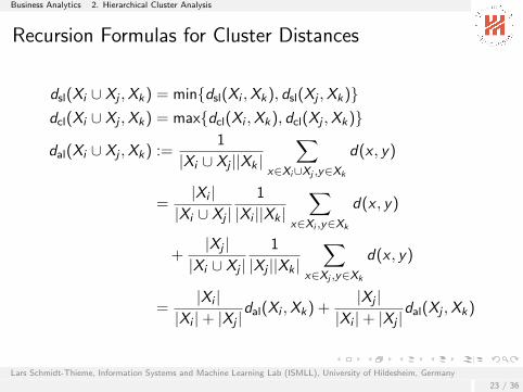
dsl(Xi ∪ Xj ,Xk) = min{dsl(Xi ,Xk), dsl(Xj ,Xk)}dcl(Xi ∪ Xj ,Xk) = max{dcl(Xi ,Xk), dcl(Xj ,Xk)}
dal(Xi ∪ Xj ,Xk) :=1
|Xi ∪ Xj ||Xk |∑
x∈Xi∪Xj ,y∈Xk
d(x , y)
=|Xi |
|Xi ∪ Xj |1
|Xi ||Xk |∑
x∈Xi ,y∈Xk
d(x , y)
+|Xj |
|Xi ∪ Xj |1
|Xj ||Xk |∑
x∈Xj ,y∈Xk
d(x , y)
=|Xi |
|Xi |+ |Xj |dal(Xi ,Xk) +
|Xj ||Xi |+ |Xj |
dal(Xj ,Xk)
agglomerative hierarchical clustering requires to compute thedistance matrix D ∈ Rn×n only once:
Di ,j := d(xi , xj), i , j = 1, . . . ,K
Lars Schmidt-Thieme, Information Systems and Machine Learning Lab (ISMLL), University of Hildesheim, Germany
23 / 36
Business Analytics 2. Hierarchical Cluster Analysis
Recursion Formulas for Cluster Distances
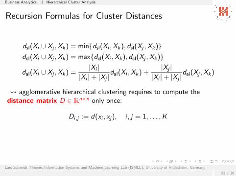
dsl(Xi ∪ Xj ,Xk) = min{dsl(Xi ,Xk), dsl(Xj ,Xk)}dcl(Xi ∪ Xj ,Xk) = max{dcl(Xi ,Xk), dcl(Xj ,Xk)}
dal(Xi ∪ Xj ,Xk) =|Xi |
|Xi |+ |Xj |dal(Xi ,Xk) +
|Xj ||Xi |+ |Xj |
dal(Xj ,Xk)
agglomerative hierarchical clustering requires to compute thedistance matrix D ∈ Rn×n only once:
Di ,j := d(xi , xj), i , j = 1, . . . ,K
Lars Schmidt-Thieme, Information Systems and Machine Learning Lab (ISMLL), University of Hildesheim, Germany
23 / 36
Business Analytics 3. Gaussian Mixture Models
Outline
1. k-means & k-medoids
2. Hierarchical Cluster Analysis
3. Gaussian Mixture Models
4. Conclusion
Lars Schmidt-Thieme, Information Systems and Machine Learning Lab (ISMLL), University of Hildesheim, Germany
24 / 36
Business Analytics 3. Gaussian Mixture Models
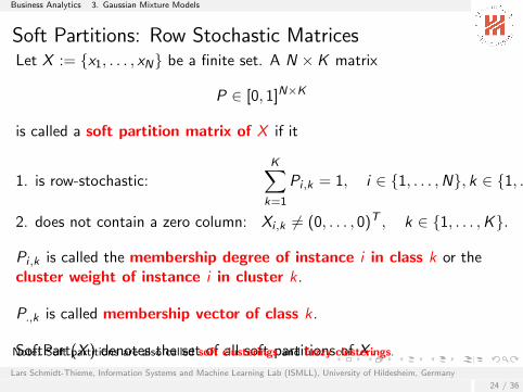
Soft Partitions: Row Stochastic MatricesLet X := {x1, . . . , xN} be a finite set. A N × K matrix
P ∈ [0, 1]N×K
is called a soft partition matrix of X if it
1. is row-stochastic:K∑
k=1
Pi ,k = 1, i ∈ {1, . . . ,N}, k ∈ {1, . . . ,K}
2. does not contain a zero column: Xi ,k 6= (0, . . . , 0)T , k ∈ {1, . . . ,K}.
Pi ,k is called the membership degree of instance i in class k or thecluster weight of instance i in cluster k .
P.,k is called membership vector of class k .
SoftPart(X ) denotes the set of all soft partitions of X .
Lars Schmidt-Thieme, Information Systems and Machine Learning Lab (ISMLL), University of Hildesheim, Germany
24 / 36
Note: Soft partitions are also called soft clusterings and fuzzy clusterings.
Business Analytics 3. Gaussian Mixture Models
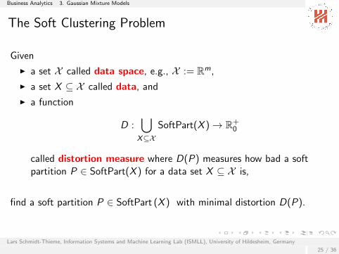
The Soft Clustering Problem
Given
I a set X called data space, e.g., X := Rm,
I a set X ⊆ X called data, and
I a function
D :⋃
X⊆XSoftPart(X )→ R+
0
called distortion measure where D(P) measures how bad a softpartition P ∈ SoftPart(X ) for a data set X ⊆ X is,
I a number K ∈ N of clusters,
find a soft partition P ∈ SoftPart (X ) with minimal distortion D(P).
Lars Schmidt-Thieme, Information Systems and Machine Learning Lab (ISMLL), University of Hildesheim, Germany
25 / 36
Business Analytics 3. Gaussian Mixture Models
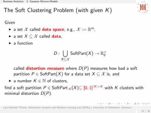
The Soft Clustering Problem (with given K )
Given
I a set X called data space, e.g., X := Rm,
I a set X ⊆ X called data,
I a function
D :⋃
X⊆XSoftPart(X )→ R+
0
called distortion measure where D(P) measures how bad a softpartition P ∈ SoftPart(X ) for a data set X ⊆ X is, and
I a number K ∈ N of clusters,
find a soft partition P ∈ SoftPart K (X )⊆ [0, 1]|X |×K with K clusters withminimal distortion D(P).
Lars Schmidt-Thieme, Information Systems and Machine Learning Lab (ISMLL), University of Hildesheim, Germany
25 / 36
Business Analytics 3. Gaussian Mixture Models
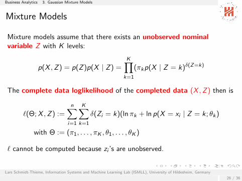
Mixture Models
Mixture models assume that there exists an unobserved nominalvariable Z with K levels:
p(X ,Z ) = p(Z )p(X | Z ) =K∏
k=1
(πkp(X | Z = k)δ(Z=k)
The complete data loglikelihood of the completed data (X ,Z ) then is
`(Θ;X ,Z ) :=n∑
i=1
K∑k=1
δ(Zi = k)(lnπk + ln p(X = xi | Z = k ; θk)
with Θ := (π1, . . . , πK , θ1, . . . , θK )
` cannot be computed because zi ’s are unobserved.
Lars Schmidt-Thieme, Information Systems and Machine Learning Lab (ISMLL), University of Hildesheim, Germany
26 / 36
Business Analytics 3. Gaussian Mixture Models
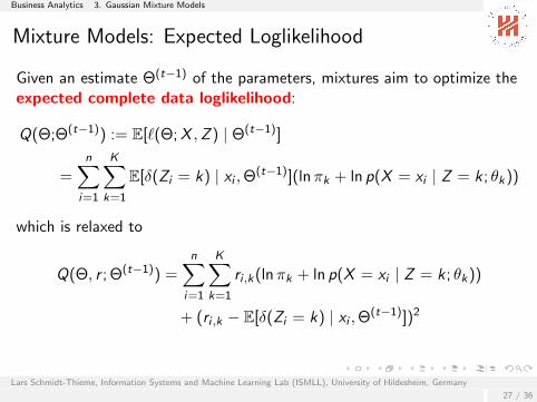
Mixture Models: Expected Loglikelihood
Given an estimate Θ(t−1) of the parameters, mixtures aim to optimize theexpected complete data loglikelihood:
Q(Θ;Θ(t−1)) := E[`(Θ;X ,Z ) | Θ(t−1)]
=n∑
i=1
K∑k=1
E[δ(Zi = k) | xi ,Θ(t−1)](lnπk + ln p(X = xi | Z = k ; θk))
which is relaxed to
Q(Θ, r ; Θ(t−1)) =n∑
i=1
K∑k=1
ri ,k(lnπk + ln p(X = xi | Z = k ; θk))
+ (ri ,k − E[δ(Zi = k) | xi ,Θ(t−1)])2
Lars Schmidt-Thieme, Information Systems and Machine Learning Lab (ISMLL), University of Hildesheim, Germany
27 / 36
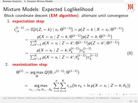
Business Analytics 3. Gaussian Mixture Models
Mixture Models: Expected LoglikelihoodBlock coordinate descent (EM algorithm): alternate until convergence
1. expectation step:
r(t−1)i ,k := E[δ(Zi = k) | xi ,Θ(t−1)] = p(Z = k | X = xi ; Θ(t−1))
=p(X = xi | Z = k ; Θ(t−1))p(Z = k ; Θ(t−1))∑K
k ′=1 p(X = xi | Z = k ′; Θ(t−1))p(Z = k ′; Θ(t−1))
=p(X = xi | Z = k ; θ
(t−1)k )π
(t−1)k∑K
k ′=1 p(X = xi | Z = k ′; θ(t−1)k )π
(t−1)k
(0)
2. maximization step:
Θ(t) := arg maxΘ
Q(Θ, r (t−1); Θ(t−1))
= arg maxπ1,...,πK ,θ1,...,θK
n∑i=1
K∑k=1
ri ,k(lnπk + ln p(X = xi | Z = k ; θk))
Lars Schmidt-Thieme, Information Systems and Machine Learning Lab (ISMLL), University of Hildesheim, Germany
28 / 36
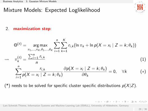
Business Analytics 3. Gaussian Mixture Models
Mixture Models: Expected Loglikelihood
2. maximization step:
Θ(t) = arg maxπ1,...,πK ,θ1,...,θK
n∑i=1
K∑k=1
ri ,k(lnπk + ln p(X = xi | Z = k ; θk))
π(t)k =
∑ni=1 ri ,kn
(1)
n∑i=1
ri ,kp(X = xi | Z = k ; θk)
∂p(X = xi | Z = k ; θk)
∂θk= 0, ∀k (∗)
(*) needs to be solved for specific cluster specific distributions p(X |Z ).
Lars Schmidt-Thieme, Information Systems and Machine Learning Lab (ISMLL), University of Hildesheim, Germany
29 / 36
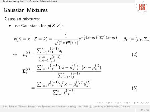
Business Analytics 3. Gaussian Mixture Models
Gaussian Mixtures
Gaussian mixtures:
I use Gaussians for p(X |Z ):
p(X = x | Z = k) =1√
(2π)m|Σk |e−
12
(x−µk )T Σ−1k (x−µk ), θk := (µk ,Σk)
µ(t)k =
∑ni=1 r
(t−1)i ,k xi∑k
i=1 r(t−1)i ,k
(2)
Σ(t)k =
∑ni=1 r
(t−1)i ,k (xi − µ
(t)k )T (xi − µ
(t)k )∑n
i=1 r(t−1)i ,k
=
∑ni=1 r
(t−1)i ,k xTi xi − µ
(t)k
Tµ(t)k∑n
i=1 r(t−1)i ,k
(3)
Lars Schmidt-Thieme, Information Systems and Machine Learning Lab (ISMLL), University of Hildesheim, Germany
30 / 36
Business Analytics 3. Gaussian Mixture Models
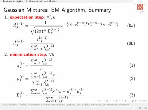
Gaussian Mixtures: EM Algorithm, Summary1. expectation step: ∀i , k
r̃(t−1)i ,k =
1√(2π)m|Σ(t−1)
k |e−
12
(xi−µ(t−1)k )T Σ
(t−1)k
−1(xi−µ(t−1)k ) (0a)
r(t−1)i ,k =
r̃(t−1)i ,k∑K
k ′=1 r̃(t−1)i ,k ′
(0b)
2. minimization step: ∀k
π(t)k =
∑ni=1 r
(t−1)i ,k
n(1)
µ(t)k =
∑ni=1 r
(t−1)i ,k xi∑n
i=1 r(t−1)i ,k
(2)
Σ(t)k =
∑ni=1 r
(t−1)i ,k xTi xi − µ
(t)k
Tµ(t)k∑n
i=1 r(t−1)i ,k
(3)
Lars Schmidt-Thieme, Information Systems and Machine Learning Lab (ISMLL), University of Hildesheim, Germany
31 / 36
Business Analytics 3. Gaussian Mixture Models
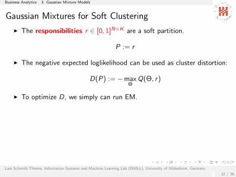
Gaussian Mixtures for Soft Clustering
I The responsibilities r ∈ [0, 1]N×K are a soft partition.
P := r
I The negative expected loglikelihood can be used as cluster distortion:
D(P) := −maxΘ
Q(Θ, r)
I To optimize D, we simply can run EM.
For hard clustering:
I assign points to the cluster with highest responsibility (hard EM):
r(t−1)i ,k = δ(k = arg max
k ′=1,...,Kr̃
(t−1)i ,k ′ ) (0b′)
Lars Schmidt-Thieme, Information Systems and Machine Learning Lab (ISMLL), University of Hildesheim, Germany
32 / 36
Business Analytics 3. Gaussian Mixture Models
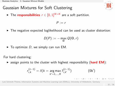
Gaussian Mixtures for Soft Clustering
I The responsibilities r ∈ [0, 1]N×K are a soft partition.
P := r
I The negative expected loglikelihood can be used as cluster distortion:
D(P) := −maxΘ
Q(Θ, r)
I To optimize D, we simply can run EM.
For hard clustering:
I assign points to the cluster with highest responsibility (hard EM):
r(t−1)i ,k = δ(k = arg max
k ′=1,...,Kr̃
(t−1)i ,k ′ ) (0b′)
Lars Schmidt-Thieme, Information Systems and Machine Learning Lab (ISMLL), University of Hildesheim, Germany
32 / 36
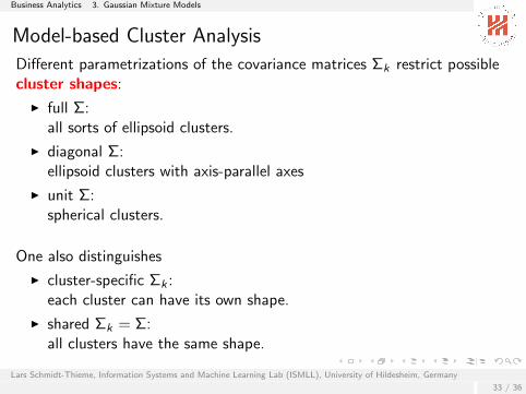
Business Analytics 3. Gaussian Mixture Models
Model-based Cluster Analysis
Different parametrizations of the covariance matrices Σk restrict possiblecluster shapes:
I full Σ:all sorts of ellipsoid clusters.
I diagonal Σ:ellipsoid clusters with axis-parallel axes
I unit Σ:spherical clusters.
One also distinguishes
I cluster-specific Σk :each cluster can have its own shape.
I shared Σk = Σ:all clusters have the same shape.
Lars Schmidt-Thieme, Information Systems and Machine Learning Lab (ISMLL), University of Hildesheim, Germany
33 / 36
Business Analytics 3. Gaussian Mixture Models
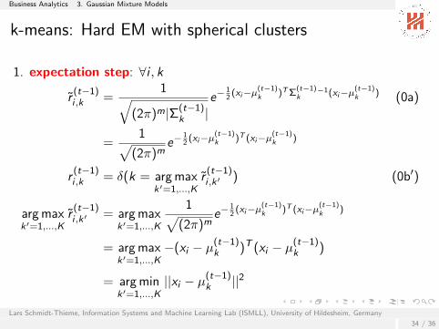
k-means: Hard EM with spherical clusters
1. expectation step: ∀i , k
r̃(t−1)i ,k =
1√(2π)m|Σ(t−1)
k |e−
12
(xi−µ(t−1)k )T Σ
(t−1)k
−1(xi−µ(t−1)k ) (0a)
=1√
(2π)me−
12
(xi−µ(t−1)k )T (xi−µ
(t−1)k )
r(t−1)i ,k = δ(k = arg max
k ′=1,...,Kr̃
(t−1)i ,k ′ ) (0b′)
arg maxk ′=1,...,K
r̃(t−1)i ,k ′ = arg max
k ′=1,...,K
1√(2π)m
e−12
(xi−µ(t−1)k )T (xi−µ
(t−1)k )
= arg maxk ′=1,...,K
−(xi − µ(t−1)k )T (xi − µ
(t−1)k )
= arg mink ′=1,...,K
||xi − µ(t−1)k ||2
Lars Schmidt-Thieme, Information Systems and Machine Learning Lab (ISMLL), University of Hildesheim, Germany
34 / 36
Business Analytics 4. Conclusion
Outline
1. k-means & k-medoids
2. Hierarchical Cluster Analysis
3. Gaussian Mixture Models
4. Conclusion
Lars Schmidt-Thieme, Information Systems and Machine Learning Lab (ISMLL), University of Hildesheim, Germany
35 / 36
Business Analytics 4. Conclusion
Conclusion (1/2)I Cluster analysis aims at detecting latent groups in data,
without labeled examples (↔ record linkage).
I Latent groups can be described in three different granularities:I partitions segment data into K subsets (hard clustering).I hierarchies structure data into an hierarchy,
in a sequence of consistent partitions (hierarchical clustering).I soft clusterings / row-stochastic matrices build overlapping groups
to which data points can belong with some membership degree (softclustering).
I k-means finds a K -partition by finding K cluster centers withsmallest Euclidean distance to all their cluster points.
I k-medoids generalizes k-means to general distances; it finds aK -partition by selecting K data points as cluster representativeswith smallest distance to all their cluster points.
Lars Schmidt-Thieme, Information Systems and Machine Learning Lab (ISMLL), University of Hildesheim, Germany
35 / 36
Business Analytics 4. Conclusion
Conclusion (2/2)
I hierarchical single link, complete link and average link methodsI find a hierarchy by greedy search over consistent partitions,I starting from the singleton parition (agglomerative)I being efficient due to recursion formulas,I requiring only a distance matrix.
I Gaussian Mixture Models find soft clusterings by modeling data bya class-specific multivariate Gaussian distribution p(X | Z ) andestimating expected class memberships (expected likelihood).
I The Expectation Maximiation Algorithm (EM) can be used tolearn Gaussian Mixture Models via block coordinate descent.
I k-means is a special case of a Gaussian Mixture ModelI with hard/binary cluster memberships (hard EM) andI spherical cluster shapes.
Lars Schmidt-Thieme, Information Systems and Machine Learning Lab (ISMLL), University of Hildesheim, Germany
36 / 36
Business Analytics
Readings
I k-means:I [HTFF05], ch. 14.3.6, 13.2.3, 8.5 [Bis06], ch. 9.1, [Mur12], ch. 11.4.2
I hierarchical cluster analysis:I [HTFF05], ch. 14.3.12, [Mur12], ch. 25.5. [PTVF07], ch. 16.4.
I Gaussian mixtures:I [HTFF05], ch. 14.3.7, [Bis06], ch. 9.2, [Mur12], ch. 11.2.3, [PTVF07],
ch. 16.1.
Lars Schmidt-Thieme, Information Systems and Machine Learning Lab (ISMLL), University of Hildesheim, Germany
37 / 36
Business Analytics
References
Christopher M. Bishop.
Pattern recognition and machine learning, volume 1.springer New York, 2006.
Trevor Hastie, Robert Tibshirani, Jerome Friedman, and James Franklin.
The elements of statistical learning: data mining, inference and prediction.The Mathematical Intelligencer, 27(2):83–85, 2005.
Kevin P. Murphy.
Machine learning: a probabilistic perspective.The MIT Press, 2012.
William H. Press, Saul A. Teukolsky, William T. Vetterling, and Brian P. Flannery.
Numerical Recipes.Cambridge University Press, 3rd edition, 2007.
Lars Schmidt-Thieme, Information Systems and Machine Learning Lab (ISMLL), University of Hildesheim, Germany
38 / 36