SM RENTALS REPORT

SM RENTALS REPORT Team 6

JLLY CONSULTING

SM RENTALS REPORT

i

EXECUTIVE SUMMARY

In order to aid the fictional organization SM Rentals, a budget car rental service, we simulated

the operation of a midsize airport location. Using data provided that pertained to the arrivals and

departures of customers, we developed a simulation model that will process the route taken by

customers as they arrive in order to discover the total amount of time that they spent in the

system. SM Rentals set a threshold of less than 18 minutes spent waiting on departure and 20

minutes upon arrival to determine satisfaction. The purpose of this case is to determine the

required resources to achieve satisfaction rates of 85% and 90%. Upon analyzing the case, we

came to the conclusion that the three significant variables determining the time that customers

spent in the system were:

1. Van Size

2. Number of Rental Counter Agents

3. Number of Drivers

Upon running multiple regression on the van size, we found that the large, 30 seat van was the

least significant and therefore removed it as an option for this model. This multiple regression

also found that the optimal number of agents and drivers for reducing the time customers spent in

the system was 18 and 16, respectively. However considering the satisfaction threshold set by

SM Rentals of 18 minutes for arrivals and 20 minutes for departures, it was possible to analyze a

smaller subset of options. 24 combinations were simulated using Arena software and their data

recorded and analyzed in Excel.

The results processed in Excel revealed that in order to meet the 85% satisfaction threshold, SM

Rentals was best served with 12 agents and drivers, while using small sized vans. The total cost

SM RENTALS REPORT

ii

of these resources is $1,743.31. This arrangement allowed for a steady flow of customers into the

rental counter, which prevented any bottlenecks that could cause customers to exceed their limit.

In order to reach the 90% threshold, 2 additional drivers were required, bringing the total number

of drivers and small vans to 14, with 12 rental counter agents. The total cost of the inputs

required is $1,932.96. The improvements yielded by the additional 2 drivers and vans were

primarily in increasing the number of drivers available at peak hours, preventing a bottleneck

from forming and allowing for more regular van service.

By using these combinations of resources, SM Rentals will be able to maintain their low cost

service while at the same time maintaining high levels of customer satisfaction. This will serve

them well as more competitors enter the markets that SM Rentals currently occupies, or if SM

Rentals intends to expand in the future. Utilizing these recommendations will allow for SM

Rentals to retain their customers and grow their customer base, which will allow for greater

revenue, and consequently more profit, in both the short- and long-term.

SM RENTALS REPORT

iii

TABLE OF CONTENTS Introduction: ................................................................................................................................................. 1

Case Background ....................................................................................................................................... 1

Challenges ................................................................................................................................................. 2

Objectives ................................................................................................................................................. 2

Limitations ................................................................................................................................................ 3

METHODS ...................................................................................................................................................... 4

Data used .................................................................................................................................................. 4

Flow of model ........................................................................................................................................... 5

Actual Model ............................................................................................................................................. 6

Metrics tracked ......................................................................................................................................... 9

Wait time ............................................................................................................................................ 10

Average Flow Time .............................................................................................................................. 10

Multi Regression Analysis ....................................................................................................................... 10

Writing into Excel .................................................................................................................................... 12

RESULTS ...................................................................................................................................................... 13

DISCUSSION ................................................................................................................................................. 15

INNOVATION IN APPROACH AND METHODOLOGY .................................................................................... 16

FURTHER CONSIDERATIONS ....................................................................................................................... 19

CONCLUSION ............................................................................................................................................... 19

APPENDIX .................................................................................................................................................... 21

SM RENTALS REPORT

iv

LIST OF FIGURES

Figure 1: Van Route ........................................................................................................................ 5

Figure 2: Create Customers ............................................................................................................ 6

Figure 3: Create Van Drivers .......................................................................................................... 7

Figure 4: Retail Counter Loading ................................................................................................... 7

Figure 5: Drop-off Station .............................................................................................................. 7

Figure 6: Terminal 1 and Terminal 2 Loading................................................................................ 8

Figure 7: Retail Counter 1............................................................................................................... 9

Figure 8: Retail Counter 2............................................................................................................... 9

Figure 9: Small Van Output .......................................................................................................... 10

Figure 10: Medium Van Output .................................................................................................... 11

Figure 11: Large Van Output ........................................................................................................ 11

Figure 12: Excel Data Summary ................................................................................................... 13

Figure 13: Simulation Results ....................................................................................................... 14

Figure 14: Drop-off Queue at the Rental Counter ........................................................................ 16

SM RENTALS REPORT

1

INTRODUCTION

Case Background This project is based on Case Competition 5 provided by Dr. Payman Jula from the IIE/RA

Contest Problems. The scenario pertains to a fictional budget car company that is facing an

increasingly challenging environment and is aiming to increase their efficiency. In order to do so

they have hired JLLY Consulting, who will simulate the processes involved in their business.

They have provided data pertaining to the arrivals from two separate terminals along with those

who are returning to the airport.

The basic premise of the model is to simulate the route taken by the vans as they travel between

the Rental Counter to the Drop-off Point, to Terminal 1, Terminal 2, and then back to the Rental

Counter. The end goal is to have a minimum of 85% satisfaction rate from the customers, which

is determined by the amount of time they spend in the system. For those arriving, this

benchmark is 20 minutes, and for those departing it is 18 minutes. The reason we will aim for an

85% satisfaction is that there will be those customers who, for various reasons, will require an

extra amount of time. We will also find what combination of variables will be necessary to

maintain a 90% satisfaction rating, and what the end cost will be for both the 85% and 90% rate.

The variables available to find the optimal model are:

1. The number of customer service agents at the Rental Counter,

2. The number of vans and corresponding van drivers,

3. The size of the vans.

The hourly cost for the customer service agents and van drivers are $11.50 and $12.50

respectively. The cost for a large, 30 seat van is $0.92/mile, a midsize, 18 seat van is $0.73/mile

SM RENTALS REPORT

2

and a small, 12 seat van is $0.48/mile. We will assume that the size of vans will be constant for

the simulation period, which is from 4:00pm to 8:30pm as outlined in the case.

Challenges This model will face a number of challenges as we work to simulate a real world scenario which

will have a variety of different factors.

One of these challenges is determining the appropriate base set of variables to use in the

simulation. Ideally, we would have some idea from the existing business of what has worked for

the business. However, this is not available. With a wide variety and combination of variables,

we will need to narrow this field.

Another challenge is the analysis of the data. Due to the structure of the model, it may be

necessary to analyze the output in another program for ease of use.

Objectives The end goal of this simulation is to manipulate the customer service agent, number of vans and

van size variables to uncover the optimal combination that will maximize customer satisfaction

and minimise the overall costs.

The benchmark for this goal is to have a minimum of 85% satisfaction by the customers, which

is determined by the amount of time they spend in the system. For those arriving, this

benchmark is 18 minutes, and for those departing it is 20 minutes. The reason we will settle for

an 85% satisfaction is that there will be those customers who for various reasons will require an

extra amount of time. We will also find what combination of variables will be necessary to

maintain a 90% satisfaction rating, and what the end cost is for both the 85% and 90%

satisfaction.

SM RENTALS REPORT

3

Limitations

Since we are using a software program to simulate events that would happen in the real world,

we must address the limitations of Arena for real world events, as well as the challenges

presented by the information presented, and not presented, in the case

Among the information deficits is the information regarding the luggage. Theoretically, a

customer with more luggage would require more time to load and disembark from the van, and

may restrict the amount of space available for other customers. However, this information was

not provided for the case, and we therefore must consider it something that will be dealt with in

future models.

Another limitation is more specific to the real world; more precisely, traffic and pedestrians.

While the model will assume the vans will travel unimpeded, this will not always be the case as

airports can be very busy. Since there is no information regarding the traffic cycles and delays,

we will assume ideal situations for the car rental vans, although this is highly unlikely.

We also must consider the role of human error in a real world situation. Since there is no way to

build this completely random element into the model, it will have to be a limitation that is

considered when implementing any findings.

Another consideration is that of back-up plans. When working with machinery, it is highly

likely that there will be some issue at various points of the day, such as the need to refuel, low air

pressure in the tires, or low oil. However, this goes beyond the scope of our model in this

iteration, and therefore can be dealt with in future models.

SM RENTALS REPORT

4

METHODS

Data used

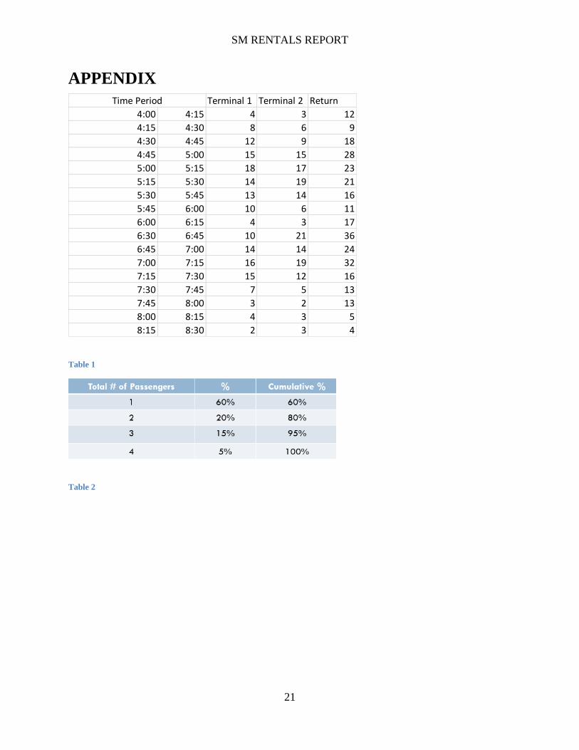
In the appendix we have provided the data set pertaining to the arrival times at the various entry

points to the model (Table 1). This data has been entered into Arena in the create entities

section. The data is focussed on the peak business period for the car rental, and therefore we will

only simulate for the peak period of 4:00pm until 8:30pm. The data is presented in intervals, with

the number of arrivals per 15 minutes.

Also included in the create entities is the likelihood that they will have a passenger with them.

60% have no passenger, 20% have 1 passenger, 15% have 2 passengers, and 5% have three

passengers. The table containing this information can be accessed in the appendix (Table 2).

In order to properly model this scenario, we needed to include the distances between the various

points that the vans would travel in the model. These distances were:

Rental Counter to Terminal 1: 1.5 miles

Rental Counter to Drop-off Point: 1.7 miles

Drop-off Point to Terminal 1: 0.5 miles

Terminal 1 to Terminal 2: 0.3 miles

Terminal 2 to Rental Counter: 2.0 miles.

Figure 1 below illustrates the route for the model:

SM RENTALS REPORT

5

Figure 1: Van Route

This data is important as the cost of the vans is based on the distance travelled, and therefore an

important component of the model.

The average speed of the vans that we will assume for the purposes of this model is 20 miles per

hour.

Flow of model The flow of model consists of customers who are returning their rented cars to the Rental

Counter arriving at the Rental Counter and meeting with the first available rental agent then

queuing for the next available van. The van will arrive, pick up all the passengers, or as many as

will fit, and then move onto the Drop-off Point where all the customers will disembark.

The van will then move to Terminal 1, pick up the customers and their passengers that are

awaiting the van, then repeat the process at Terminal 2 until all the customers are picked up, or

there are no more available seats.

From here, the van will return to the Rental Counter where the passengers will disembark and the

van will collect the next group of passengers and repeat the process, beginning with the Drop-off

SM RENTALS REPORT

6

Point (unless there are no customers waiting, in which case it will proceed directly to Terminal

1).

Those who have arrived with the van to the Rental Counter will proceed inside, and will queue

up for the next available agent. When they have been served by the agents present, they will

then move on and out of the system with their rental car.

These processes will repeat for the time period of 4:30 until 8:30.

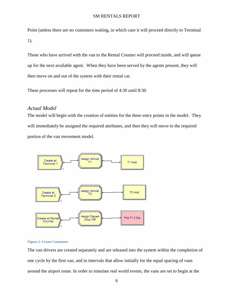
Actual Model The model will begin with the creation of entities for the three entry points in the model. They

will immediately be assigned the required attributes, and then they will move to the required

portion of the van movement model.

Figure 2: Create Customers

The van drivers are created separately and are released into the system within the completion of

one cycle by the first van, and in intervals that allow initially for the equal spacing of vans

around the airport route. In order to simulate real world events, the vans are set to begin at the

SM RENTALS REPORT

7

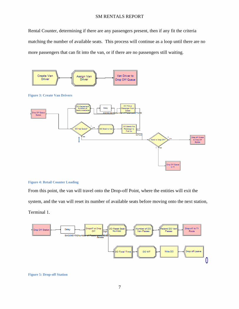
Rental Counter, determining if there are any passengers present, then if any fit the criteria

matching the number of available seats. This process will continue as a loop until there are no

more passengers that can fit into the van, or if there are no passengers still waiting.

Figure 3: Create Van Drivers

Figure 4: Retail Counter Loading

From this point, the van will travel onto the Drop-off Point, where the entities will exit the

system, and the van will reset its number of available seats before moving onto the next station,

Terminal 1.

Figure 5: Drop-off Station

SM RENTALS REPORT

8

At Terminal 1, it will repeat the same procedure that it did with the Drop-off Point, determining

if there are passengers waiting, and then if there are any that will fit into the remaining seats.

Upon satisfying this procedure, it will move on to Terminal 2 and repeat the procedure once

more. Then it will return to the Rental Counter.

Figure 6: Terminal 1 and Terminal 2 Loading

At the Rental Counter, the van will empty and reset its seats, then load up passengers waiting to

be dropped back off at the airport, and repeat its path. For those who have just disembarked

from the van, they will proceed to the Rental Counter, where they will queue up at the rental

counter alongside passengers who are returning their cars and dropping off their keys. After

getting processed by the agent at the rental counter, all the customer entities will pass through a

decision that will distinguish them from those who have picked up their car (arrived at T1 and

T2), and those who have just dropped off their car (needs to be dropped off). Those who have

picked up their car will proceed to leave the rental counter and depart from the system.

SM RENTALS REPORT

9

Customers who have dropped off their cars and needs to be dropped back off at the airport will

queue up for a van, which will take them back to the airport to be dropped off and disposed off.

Figure 7: Retail Counter 1

Figure 8: Retail Counter 2

If there are no customers lined up at the rental counter to get dropped, the van will proceed from

the rental counter directly to T1, bypassing the Drop-off Area. It is important to note that if there

are no passengers waiting at a station, the van will proceed straight through, as they would in a

real world situation.

Metrics tracked In order to gain an understanding of what the model illustrates, there was a variety of data

captured from the simulations.

SM RENTALS REPORT

10

Wait time

Since wait time is a key portion of the model’s end goals, it was important to record these

statistics for analysis. The wait time consists of the time that the customer spent within the

system, from arrival to departure. This was collected under a variety of different scenarios, using

a different combination of agents, van sizes, and number of drivers each time.

Average Flow Time

Average flow time was captured in order to illustrate the amount of time the entity spent in the

system from creation to disposal.

Multi Regression Analysis

Running this module, it was found that the 30-seat van was negligible, with results that were

highly similar to the 18-seat van. Therefore, the simulation will be limited to testing variations

of inputs with the small and medium sized vans.

Figure 9: Small Van Output

SM RENTALS REPORT

11

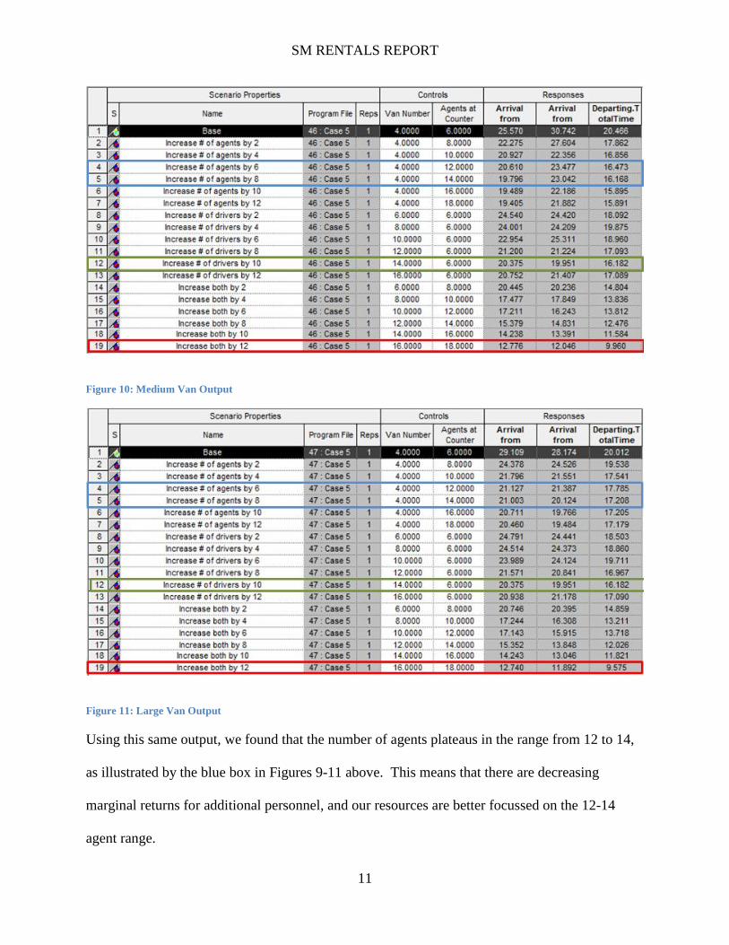
Figure 10: Medium Van Output

Figure 11: Large Van Output

Using this same output, we found that the number of agents plateaus in the range from 12 to 14,

as illustrated by the blue box in Figures 9-11 above. This means that there are decreasing

marginal returns for additional personnel, and our resources are better focussed on the 12-14

agent range.

SM RENTALS REPORT

12

The drivers’ output shows that the number of drivers that will minimize time is 13, as illustrated

in Figures 9-11 above in the green box. However, we will analyze more options around this

number in order to ascertain the best option.

It is important to note that the goal of this model is not solely minimizing time however; we must

also consider the cost of the inputs required to reduce the time.

Based off this information, we will run simulations for 24 different variations of the

small/medium size vans, number of drivers, and number of agents. The goal of the combinations

will be to satisfy the 85%, and 95%, satisfaction rates while minimizing the costs.

In order to ensure accuracy, we will run each simulation for 5 days, and take the average from

this set of 5.

Writing into Excel

In order to summarize the information produced by the model, we utilized the Write module in

Arena to copy the data into Excel. In particular, we focussed on the total time the customers

spent within the system in order to test the satisfaction levels with each combination of variables.

From Excel, we will then average the data points collected from each run of the model, and bin

them in order to determine the distribution and test their satisfaction against the standards we

have set. Figure 12 below illustrates the summary of data for one combination of variables.

SM RENTALS REPORT

13

Figure 12: Excel Data Summary

As shown above, the time is averaged, and the distribution is shown in the bins below, along

with the total number of customers that were in the system for the simulation. The satisfaction

rate is found by summing the total number customers that were under the time limit, and then

divided by the total count.

For instance, the arrival bins 0, 5, 10, 15, and 20 have values that sum to 1,357. Divide this

value by the total count, 1656, and the satisfaction rate is 81.9%.

RESULTS

Referring to Figure 13 below, we can see the outcome for the 24 simulated scenarios.

It is immediately apparent from looking at the satisfaction section that the least expensive

combination for a minimum of 85% satisfaction is combination 3, with 87.9% satisfaction for

arrivals and 91.72% for departures. This entails:

Arrival Dropoff

Avg. time in system: 15.54439 12.49364

Bins # Bins #

0 0 0 0

5 0 5 0

10 108 10 501

15 755 15 573

20 494 18 208

25 253 25 183

30 45 30 0

Count 1656 1465

Sat. Rate 0.819444 0.875085

SM RENTALS REPORT

14

Van = Small (Fuel Cost = $447.31)

12 Drivers (Wages = $675)

12 Agents (Wages = $621)

Total cost $1,743.31

In order to satisfy the 90% satisfaction goal, combination 11 is the least expensive option. This

provides a satisfaction rate of 95.17% for arrivals and 95.96% for departures. The variables are:

Van = Small (Fuel Cost = $524.46)

14 Drivers (Wages = $787.50)

12 Agents (Wages = $621.00)

Total Cost = $1,932.96

Figure 13: Simulation Results

<= 20 Mins <= 18 Mins

Comb. # Car Types Fuel Costs #s of Drivers Cost #s of Agents Cost Total Cost Satisfaction Rate for Arrival Satisfaction Rate for DO

1 Small (12) 403.82$ 11 618.75$ 12 621.00$ 1,643.57$ 81.94% 87.51%

2 Small (12) 403.82$ 11 618.75$ 13 672.75$ 1,695.32$ 82.44% 87.98%

3 Small (12) 447.31$ 12 675.00$ 12 621.00$ 1,743.31$ 87.92% 91.72%

4 Small (12) 403.82$ 11 618.75$ 14 724.50$ 1,747.07$ 82.67% 87.09%

5 Small (12) 447.31$ 12 675.00$ 13 672.75$ 1,795.06$ 87.79% 89.96%

6 Small (12) 490.00$ 13 731.25$ 12 621.00$ 1,842.25$ 89.20% 91.64%

7 Small (12) 447.31$ 12 675.00$ 14 724.50$ 1,846.81$ 87.69% 90.01%

8 Medium (18) 612.45$ 11 618.75$ 12 621.00$ 1,852.20$ 78.76% 85.71%

9 Small (12) 490.00$ 13 731.25$ 13 672.75$ 1,894.00$ 85.59% 88.42%

10 Medium (18) 612.45$ 11 618.75$ 13 672.75$ 1,903.95$ 82.00% 88.16%

11 Small (12) 524.46$ 14 787.50$ 12 621.00$ 1,932.96$ 95.17% 95.96%

12 Small (12) 490.00$ 13 731.25$ 14 724.50$ 1,945.75$ 89.68% 91.10%

13 Medium (18) 612.45$ 11 618.75$ 14 724.50$ 1,955.70$ 82.61% 87.44%

14 Medium (18) 683.55$ 12 675.00$ 12 621.00$ 1,979.55$ 85.52% 90.96%

15 Small (12) 524.46$ 14 787.50$ 13 672.75$ 1,984.71$ 92.75% 94.19%

16 Medium (18) 683.55$ 12 675.00$ 13 672.75$ 2,031.30$ 88.29% 90.97%

17 Small (12) 524.46$ 14 787.50$ 14 724.50$ 2,036.46$ 93.05% 94.53%

18 Medium (18) 683.55$ 12 675.00$ 14 724.50$ 2,083.05$ 89.67% 92.48%

19 Medium (18) 738.64$ 13 731.25$ 12 621.00$ 2,090.89$ 92.10% 94.19%

20 Medium (18) 738.64$ 13 731.25$ 13 672.75$ 2,142.64$ 92.39% 93.01%

21 Medium (18) 738.64$ 13 731.25$ 14 724.50$ 2,194.39$ 91.62% 92.95%

22 Medium (18) 796.92$ 14 787.50$ 12 621.00$ 2,205.42$ 90.27% 92.11%

23 Medium (18) 796.92$ 14 787.50$ 13 672.75$ 2,257.17$ 92.82% 94.19%

24 Medium (18) 796.92$ 14 787.50$ 14 724.50$ 2,308.92$ 92.03% 92.68%

Outcomes

SM RENTALS REPORT

15

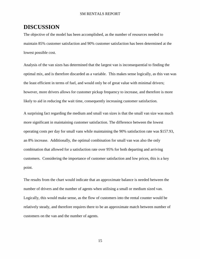
DISCUSSION

The objective of the model has been accomplished, as the number of resources needed to

maintain 85% customer satisfaction and 90% customer satisfaction has been determined at the

lowest possible cost.

Analysis of the van sizes has determined that the largest van is inconsequential to finding the

optimal mix, and is therefore discarded as a variable. This makes sense logically, as this van was

the least efficient in terms of fuel, and would only be of great value with minimal drivers;

however, more drivers allows for customer pickup frequency to increase, and therefore is more

likely to aid in reducing the wait time, consequently increasing customer satisfaction.

A surprising fact regarding the medium and small van sizes is that the small van size was much

more significant in maintaining customer satisfaction. The difference between the lowest

operating costs per day for small vans while maintaining the 90% satisfaction rate was $157.93,

an 8% increase. Additionally, the optimal combination for small van was also the only

combination that allowed for a satisfaction rate over 95% for both departing and arriving

customers. Considering the importance of customer satisfaction and low prices, this is a key

point.

The results from the chart would indicate that an approximate balance is needed between the

number of drivers and the number of agents when utilising a small or medium sized van.

Logically, this would make sense, as the flow of customers into the rental counter would be

relatively steady, and therefore requires there to be an approximate match between number of

customers on the van and the number of agents.

SM RENTALS REPORT

16

INNOVATION IN APPROACH AND METHODOLOGY

Because we chose to model our vans using entities, we had to come up with a way that would

allow for the customers (also entities) to travel with the van-entity. We chose to use a Hold

module to represent the passenger entities queuing up for a van at T1, T2 and at the Rental

Counter waiting to get dropped off. The methodology that we decided to use involves a search

and pick loop, where the van will travel through the loop, picking up as many passengers as

possible, and then exiting the loop.

Figure 14: Drop-off Queue at the Rental Counter

For example, in the Drop-off Queue at the Rental Counter Loop the van-entity will enter the

station and reach the decision node. The decision node contains the expression ((NQ(Drop Off

Hold.Queue))>0) && (Seats>0), asking if the length of Drop Off Hold.Queue is greater than 0

(is there someone in the queue?) and if the van-entity’s seat-attribute is greater than 0 (does my

van have at least 1 empty seat?). If both conditions are satisfied, the van-entity will proceed to

assign a variable, in this case DO Seats Var, to be equal to its current Seats-attribute. This step is

necessary because the search module following it requires that a variable be used in its search

condition.

SM RENTALS REPORT

17

The van-entity then reaches the search module, where we have specified that it is to search

through the entire Drop Off Hold.Queue (NQ = length of queue), and to assign the letter-variable

J to the first entity in the queue that satisfies the search condition (Number of Passengers <= DO

Seats Var), meaning the first customer-entity in the queue whose number of passengers-attribute

is less than or equal to the number of seats available in the van. This equation gives us the

advantage of being able to bypass a customer-entity if their number of passengers exceeds the

seats available, and pick up the next customer-entity whose number of passengers is equal to or

less than the number of seats available, reflecting the real-world situation. If none of the

customer-entity fulfill the requirement (all of the customers have more passengers than the

number of seats available), they will exit the loop.

The van-entity then picks up the customer-entity that we have identified and labeled in the search

condition with the variable J. Following the pickup, there is a delay for the boarding time in the

van. This is represented by a Delay block, with the delay time being AG(NG,NSYM(Number of

Passengers))*12/60. As the most recent entity picked up joins the end of the group, the Delay

time formula specifies that we want to find the number of passengers-attribute from the last

entity in the group (NG = group size), and multiply it by 12 seconds for boarding time. We then

also have to divide the formula by 60 seconds since our base unit is in minutes.

The usage of a Delay block, which is almost at the lowest level of building blocks in Arena,

rather than using a Delay module or even accounting for delay in the Leave modules is because

this method allows for a more accurate animation of delay. Using the other two modules listed

above will cause the van-entity to disappear from the animation while the delay is taking place.

The Delay block allows for the input of a Storage ID, allowing us to create a Storage and place

SM RENTALS REPORT

18

one on the animation, thus creating a place for the animated van-entity to be stored at while the

delay is taking place.

Next, the Assign module allows for the Seats-attribute of the Van-entity to be decreased, to

reflect the updated number of seats available. The Seats-attribute is assigned a new value of

Seats -AG(NG,NSYM(Number of Passengers)), which means current seats available minus the

number of passengers-attribute from the last customer-entity that we just picked up. The van will

then proceed to the decision node again, and the loop will continue.

If the conditions of the decision node are not met, or if the van-entity is unsuccessful in its search

for a customer-entity whose passenger number-attribute meets the search condition requirements,

the van-entity (and all the customer-entity grouped with it) exits the loop.

In the beginning of Van Driver Creation, we also assigned another attribute, Seats Constant, to

the van driver to track whether the van needs to proceed to the Drop Off area after the Rental

Counter, or if they can go directly to T1. The Decision node asks if number of Seats in van <

Seats Constant, meaning whether the number of available seats in the van is less than the number

of seats that are supposed to be in the van. If the number of seats in the van is less than Seats

Constant, this indicates that there is at least one customer-entity in the van, and so it would

therefore route the van-driver to the Drop-off Area to drop off the customer-entity.

Seats Constant is also used to reset the number of seats in the van following the drop-off of the

customer-entities at either the Rental Counter (for arrivals at T1 and T2) or the Drop-off Area

(departures).

SM RENTALS REPORT

19

FURTHER CONSIDERATIONS

It is important to note that there are additional costs to consider when implementing this model

that are not included here. Among the most significant is that with the use of small vans, SM

Rental will be required to purchase more vehicles than if they were to utilize medium or large

vans. There will also be more vehicles to maintain, and this would likely increase the

maintenance costs.

Additionally, with more vehicles used, SM Rentals will need to hire more drivers, which will

cost them additional resources as they train these new employees.

Both of these costs were not included in the model, but should require some consideration before

implementation.

Another consideration should be valuing the marginal increase in satisfaction with different

combinations and costs. While we have ascertained that there is an 8% increase in cost in order

to gain a further 5% satisfaction (from 85% to 90%), it could be illuminating to gain a clearer

picture of what the marginal cost is at different levels. This would require further simulations

and further analysis beyond the scope of this report.

CONCLUSION

SM Rental is best served with the use of a small van and 12 agents and drivers if they wish to

accomplish a satisfaction rate of 85%, assuming they maintain their threshold of 18 minutes in

the system for those arriving and 20 minutes for those departing. This will amount to a total cost

of $1,743.31.

SM RENTALS REPORT

20

If they wish to maintain a 95% satisfaction rate, they will instead require 12 agents, 14 drivers

while still using the small van. The total cost for this combination of resources is $1,932.96.

Again, this holds the satisfaction thresholds of 18 and 20 minutes constant.

These two options detail different approaches for SM Rentals. The difference between the

simulated cost for 90% customer satisfaction and 85% customer satisfaction is $157.93, or an 8%

increase in cost. This will be something that SM Rentals should consider as they debate the

benefits of the extra 5% satisfaction.

Overall, this gives SM Rentals meaningful results that they can apply to improve the

performance of their service in terms of customer satisfaction.

SM RENTALS REPORT

21

APPENDIX

Table 1

Table 2

Terminal 1 Terminal 2 Return

4:00 4:15 4 3 12

4:15 4:30 8 6 9

4:30 4:45 12 9 18

4:45 5:00 15 15 28

5:00 5:15 18 17 23

5:15 5:30 14 19 21

5:30 5:45 13 14 16

5:45 6:00 10 6 11

6:00 6:15 4 3 17

6:30 6:45 10 21 36

6:45 7:00 14 14 24

7:00 7:15 16 19 32

7:15 7:30 15 12 16

7:30 7:45 7 5 13

7:45 8:00 3 2 13

8:00 8:15 4 3 5

8:15 8:30 2 3 4

Time Period