burlington street bridge in iowa city on june 30, 2014 ... · question #2: neral, was the monthly...

WOC Flash Flood Simulation Application #1

Burlington Street Bridge in Iowa City on June 30, 2014

(Photo Credit: Adam Wesley/The Gazette-KCRG-TV9)

Warning Operations Course: Flash Flood

Simulation Application #1 Hydrometeorological Forecasting

June 30 – July 1, 2014 Des Moines, IA event

Designed by the National Weather Service

WARNING DECISION TRAINING DIVISION (WDTD) Office of the Chief Learning Officer (OCLO)

Release Date: March 2017

http://whotv.com/2014/07/02/latest-crest-forecast-road-trail-closures/


Table of Contents (Labels are clickable links to navigate to that section)

I. Introduction ...............................................................................................................................3

II. Receiving Credit ..........................................................................................................................3

III. Simulation Details ......................................................................................................................4

IV. Starting the Simulation ...............................................................................................................4

V. Performance Objectives ..............................................................................................................5

1. Antecedent Conditions/Topography ........................................................................................5

2. Synoptic Pattern Analysis ...................................................................................................... 10

3. Meteorological Ingredients ................................................................................................... 14

4. Standardized Anomalies ........................................................................................................ 20

5. Quantitative Precipitation Forecasts (QPFs) ........................................................................... 23

6. Write an Area Forecast Discussion (AFD) ............................................................................... 24


I. Introduction Simulation Application #1 is a displaced real-time simulation within the Des Moines, IA county warning area (CWA). The primary goal of this simulation application is to apply the learning objectives from training modules into forecasting the heavy rainfall and flash flood potential for the Des Moines CWA. The trainee will use forecast model data, including forecast standard anomalies and quantitative precipitation forecasts (QPFs), throughout the analysis. The trainee then applies the analyses to write an Area Forecast Discussion (AFD) describing the heavy rain and flash flood potential over the F000-F036 hour forecast period. Defining effective performance objectives and evaluation criteria are essential to a successful simulation. The performance objectives outlined here (and in the embedded quizzes) coincide with the learning objectives from the WOC Flash Flood Track. However, the facilitator is encouraged to enhance the learning experience by creating supplemental objectives that tailor the training to any specific needs at their office. The student should have a clear understanding of the objectives prior to starting the simulation.

II. Receiving Credit In order to receive credit for Simulation Application #1, the trainee must pass all five quizzes embedded in the recorded presentation within the WESSL script. At the end of each quiz, there is a code that should be written down. Upon completion of Simulation Application #1, the trainee must log into the LMS, navigate to the lesson “Flash Flood Simulation #1 - DMX”, and provide the five codes in order to be marked complete. Additionally, the final performance objective requires that the trainee write an Area Forecast Discussion (AFD), to be reviewed by his/her facilitator. We encourage both the trainee and facilitator to discuss the AFD, as this is the most operationally relevant component of this section. However, there is no trackable completion requirement for the AFD.


III. Simulation Details WFO Localization Des Moines, IA (DMX) Simulation Start Date/Time June 29, 2014 – 1400 UTC Simulation End Date/Time June 29, 2014 – 1600 UTC Case Name Hydro Case WFO Capability AWOC FF WESSL Script WOC_Flash_Flood_Sim_Application_1 Simulation Mode Displaced Real-Time Estimated Completion Time 90 minutes (NOTE: While we expect this

exercise to take 90 minutes, we provide an additional 30 minutes of simulation time in case some forecasters take longer to perform the prescribed analyses)

IV. Starting the Simulation In the upper-left corner of the WES-2 Bridge desktop, navigate to the Applications menu, and then the WDTD submenu. Click “WDTD Training Resources” (see figure below).

Figure. Link to the WDTD Training Resources webpage.


By clicking this button, a Firefox web browser will open a local web page with a link to “WOC Flash Flood Simulation Documents” (see figure below). Clicking this link will lead you to supplemental documentation for this course, including a PDF titled “Instructions for Launching Simulations”. Please refer to this document for details on how to load, launch, and start the simulation.

Figure. WDTD Training Resources webpage, with links to supplemental documentation.

V. Performance Objectives

1. Antecedent Conditions/Topography Evaluate the antecedent soil moisture profile and recent precipitation that can impact the flash flood potential in the Des Moines county warning area (CWA). Also evaluate the topographic features of the Des Moines CWA. Evaluation Criteria 1.1 – First, we will evaluate the precipitation that the area received during May 2014. Figure 1 shows the NWS Advanced Hydrologic Prediction Service (AHPS) total observed precipitation for the month of May 2014. Figure 2 shows the percent of normal precipitation for the month of May 2014. For more information about these plots, visit: http://water.weather.gov/precip/

Question #1: Approximately how much rain fell in central Iowa in the month of May?

http://water.weather.gov/precip/


Question #2: In general, was the monthly precipitation for central Iowa above or below normal, based on Figure 2?

Figure 1. NWS Advanced Hydrologic Prediction Service (AHPS) Monthly Observed Precipitation for May 2014.

Figure 2. NWS Advanced Hydrologic Prediction Service (AHPS) Monthly Percent of Normal Precipitation for May 2014.


Evaluation Criteria 1.2 – Now we will analyze the soil moisture content and anomalies. Figure 3 contains the calculated soil moisture ranking percentile at the end of May 2014. For more information about this plot, visit: http://www.cpc.ncep.noaa.gov/products/Soilmst_Monitoring/US/Soilmst/Soilmst.shtml

Question #1: Describe the predominant soil moisture conditions for central Iowa, based on the ranking percentile data.

Question #2: Based on your analyses of the precipitation totals and soil moisture for May, how would you describe the flash flood potential going into June?

Figure 3. NWS Climate Prediction Center (CPC) Calculated Soil Moisture Ranking Percentile for May 2014. Warm colors denote below average soil moisture, while cool colors denote above average soil moisture.

http://www.cpc.ncep.noaa.gov/products/Soilmst_Monitoring/US/Soilmst/Soilmst.shtml

http://www.cpc.ncep.noaa.gov/products/Soilmst_Monitoring/US/Soilmst/Soilmst.shtml


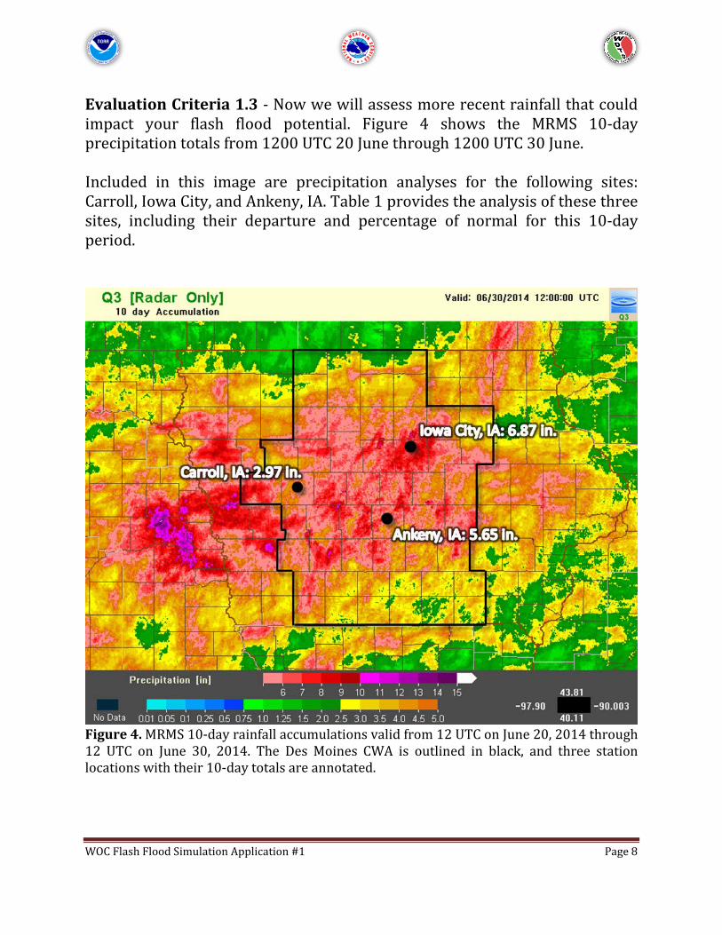
Evaluation Criteria 1.3 - Now we will assess more recent rainfall that could impact your flash flood potential. Figure 4 shows the MRMS 10-day precipitation totals from 1200 UTC 20 June through 1200 UTC 30 June. Included in this image are precipitation analyses for the following sites: Carroll, Iowa City, and Ankeny, IA. Table 1 provides the analysis of these three sites, including their departure and percentage of normal for this 10-day period.

Figure 4. MRMS 10-day rainfall accumulations valid from 12 UTC on June 20, 2014 through 12 UTC on June 30, 2014. The Des Moines CWA is outlined in black, and three station locations with their 10-day totals are annotated.


Location Observed Precip

Normal Precip

Departure from Normal

Percentage of Normal

Carroll, IA 2.97 in. 1.70 in. +1.27 in. +175% Iowa City, IA 6.87 in. 1.82 in. +5.05 in. +377% Ankeny, IA 5.65 in. 1.72 in. +3.93 in. +328% Table 1. 10-day precipitation analyses (valid during the same time as Figure 4) for three sites within the Des Moines CWA.

Question #1: Within the Des Moines CWA, how do the 10-day totals in Figure 4 compare to the May totals? Question #2: Using the site data from Table 1, was the total precipitation from 1200 UTC 20 June to 1200 UTC 30 June above or below the average precipitation for this period? Question #3: We will now evaluate the rarity of Iowa City’s 10-day total in terms of Average Recurrence Intervals (ARIs). Figure 5 shows the ARIs for an Iowa City station, including 90% confidence intervals under each frequency estimate. For more information about this table, visit: http://hdsc.nws.noaa.gov/hdsc/pfds/index.html Using information from Figure 5, how would you describe the rarity of Iowa City’s 10-day total of 6.87”? Question #4: What impact would this precipitation have on the soil moisture content and future flash flood potential?

Evaluation Criteria 1.4 - In CAVE, set a pane to the “WFO” scale and load the “HighRes Topo Image” from the Maps menu. You can also load the “CWAs” product to help delineate the Des Moines CWA.

Question #1: How could the topographic features of DMX impact the flash flood and runoff potential?

http://hdsc.nws.noaa.gov/hdsc/pfds/index.html


Figure 5. Average recurrence intervals (ARIs; in years) from the NOAA Atlas 14 Point Precipitation Frequency Estimates for Iowa City, IA, managed by the NWS Hydrometeorological Design Studies Center.

2. Synoptic Pattern Analysis Evaluate the synoptic-scale pattern for a short-term forecast (F000-F036 hour period) using the available model data from the GFS. This performance objective applies the research performed by Maddox et al. (1979) on identifying basic synoptic-scale patterns associated with heavy rainfall and flash flood events. A “top-down” synoptic-scale analysis will be performed on the 250 mb, 500 mb, the 850 mb constant pressure level charts,


as well as the surface. Afterwards, the student will then identify which Maddox pattern(s) exist and how the synoptic setup evolves. Throughout this section, hand analysis may be completed (using Figure 6) to aid in the student’s understanding. Use the “Procedures Details” PDF to see detailed information about each procedure in this section. Evaluation Criteria 2.1 - Load the 250mbAnalysis procedure from the SimApp1 procedure bundle.

Question #1: Focusing on the F000-F036 period, look through the GFS model loop forecast for the 250 mb constant pressure level. Consider the evolution of pressure waves and jet streams affecting the Des Moines CWA over this forecast period. Identify the jet max at F030 hour. Question #2: Between F030 and F036, how could you interpret the location of the Des Moines CWA, as it relates to the jet max axis? [Hint: use the four-quadrant model.]

Evaluation Criteria 2.2 - Load the 500mbAnalysis procedure from the SimApp1 procedure bundle.

Question #1: Focusing on the F000-F036 period, look through the GFS model loop for the 500 mb constant pressure level. Be sure to toggle between 500 mb wind speed and dew point depressions ≤ 6°C. Describe the evolution of the pressure waves and areas of dew point depressions ≤ 6°C.

Evaluation Criteria 2.3 - Load the 850mbAnalysis procedure from the SimApp1 procedure bundle.

Question #1: Focusing on the F000-F036 period, look through the GFS model loop for the 850 mb constant pressure level. Consider the evolution of pressure waves and dew point temperatures ≥ 10°C affecting the Des Moines CWA. Over the forecast period, describe the axis of greatest 850 mb


winds (i.e. the low-level jet) as it relates to moisture flux near the Des Moines CWA.

Evaluation Criteria 2.4 - Load the SurfaceAnalysis procedure from the SimApp1 procedure bundle.

Question #1: Focusing on the F000-F036 period, look through the GFS model loop for the surface. Consider the evolution of air masses, fronts, and dew point temperatures ≥ 60°F affecting the Des Moines CWA. Over the forecast period, identify highs/lows, fronts, general surface flow, and areas of dew point temperatures ≥ 60°F.

Evaluation Criteria 2.5 – You have now completed your top-down analysis. Recall the IC1 Conceptual Models lesson on heavy rainfall and flash flood synoptic-scale patterns (Lesson 1).

Question #1: Which Maddox heavy rainfall pattern best represents the set-up analyzed at F030 hour? Question #2: Based on your top-down analysis, identify the region that you would expect to contain the greatest rainfall potential at F030 hour (18Z on June 30, 2014).


Figure 6. Blank map for hand analysis, if needed for the synoptic pattern analyses.


3. Meteorological Ingredients Apply ingredients-based methodologies and sounding analysis in the short-term forecast (F000-F036 hour period) using the available model data to evaluate the favorability of heavy rainfall ingredients. This performance objective applies the research by Junker et al. (1999) on how to use an ingredients-based approach to estimate the scale and intensity of heavy rainfall events (recall IC1 Conceptual Models: Lesson 2). The student will evaluate several meteorological ingredients and interpret sounding data to determine the extent of forecasted heavy rainfall. Load the “MoistureAnalysis” procedure from the SimApp1 procedure bundle. This is a four-panel procedure that you will use throughout this performance objective. Use the “Procedures Details” PDF to see detailed information about this procedure. Evaluation Criteria 3.1 – We will first evaluate the moisture/temperature transport and moisture flux convergence with respect to the work by Junker et al. (1999). Start with Panel #1, which contains the 850 mb winds, 850 mb moisture transport, 850 mb equivalent potential temperature, and surface wind streamlines. Step through the F000-F036 hour forecast period.

Question #1: Junker et al. found that the heaviest rainfall in the events they observed fell downwind (N or NE) of the axis of greatest 850 mb winds and moisture flux in the area of 850 mb Ɵe. Based on this, where should the heaviest rainfall occur at F030? Question #2: Look at the 850 mb moisture transport at F030 hour. Consider the extent of the moisture transport axis (width, location, movement). Describe the axis characteristics at F030, and whether they support a heavy rainfall event.

Rotate over to Panel #2. We will now discuss how the 850 mb moisture transport relates to the 850 mb moisture flux convergence. [NOTE: the


AWIPS-2 product is Moisture Flux Divergence. Thus, negative values will show areas of convergence.]

Question #3: At the F030 hour, toggle between viewing the 850 mb Moisture Transport Magnitude and 850 mb Moisture Flux Divergence products. Recall the schematic from IC1 Lesson 2. Does the set-up at F030 match the diagram, indicating a favorable set-up for a heavy rain event?

Evaluation Criteria 3.2 – We will now evaluate the magnitude of the available moisture in the atmosphere, using findings from Funk (1991). Figure 7 shows a chart with precipitable water values on the x-axis and 1000-500 mb thickness on the y-axis. The line shown in the graph is the 70% saturation thickness line defined by Funk (1991). Any point to the right of the line is assumed to have a mean relative humidity around or above 70%. The work by Funk (1991) showed that heavy rainfall events can have values near the 70% saturation thickness level with the most significant heavy rainfall events having values above the 70% saturation thickness level. Rotate to Panel #3. This procedure contains an image combination of precipitable water greater than 1.00 inch and 1000-500 mb mean relative humidity greater than 70%. Turn on sampling.

Question #1: For F030, plot the model precipitable water value vs. the model-estimated 1000-500 mb thickness near Des Moines, IA on the plot given in Figure 7. Question #2: Describe the potential for heavy rainfall based on this analysis. NOTE: You may toggle to the mean relative humidity product to help with this question. Values are also available if sampling is on.


Figure 7. Blank plot of precipitable water (PW) along the x-axis and 1000-500 mb thickness (dm) along the y-axis. Annotated line is the 70% saturation thickness defined by Funk (1991). Evaluation Criteria 3.3 - Now we will examine some forecast point soundings within the Des Moines CWA.

1. Switch to a new pane. 2. Set the zoom to “State Scale.” 3. In the Maps menu, add the “Cities” map.

a. Set the map density to 0.33, so you just see the major cities. 4. Go to the Tools menu and click on the “Points” tool. 5. Right-click “Interactive Points” in the lower right, and click “Edit

Points…” 6. In the Points List window, highlight Point A and click “Edit…” 7. Set the coordinates of Point A to:

a. Lat: 41° 34’ 36.123” N b. Lon: 93° 37’ 3.465” W


8. Open the Volume Browser. 9. To the right of the Tools menu (across the top left of the window),

change the product type to “Sounding”. 10. Select “GFS40” from Sources Volume. 11. Create a sounding for Point A.

You may use Table 2 to help keep track of your analyses. NOTE: The forecast times are located in the far right upper panel of the NSHARP editor tab.

Question #1: Describe the vertical moisture profile of the sounding at 1800 UTC on June 30.

Question #2: What are the heights of the LCL and Freezing Level at 1800 UTC on June 30? What is the Warm Cloud Layer at 1800 UTC on June 30? Question #3: Using your Warm Cloud Layer depth from the previous question, is this a favorable condition for heavy precipitation? Why? Question #4: What is the direction and magnitude (in kts) of the SFC-6 km mean wind (MnWind) at 1800 UTC on June 30? Question #5: What does this SFC-6 km mean wind tell you about the potential for heavy rainfall? Question #6: Is the CAPE profile supportive of heavy precipitation at 1800 UTC on June 30? Question #7: What is the precipitable water (PW) value (in inches) at 1800 UTC on June 30?


Skew-T Parameter 1800 UTC 30 June 2014 Moisture Profile: Describe the vertical moisture profile of the GFS40 sounding.

LCL Height: Write down the values of LCL (in mb and feet). Use the sounding sampling at the height of the green LCL line.

Height of the Freezing Level: Write down the value of FZL (in feet).

Warm Cloud Layer: Determine the depth of the warm cloud layer (in feet). Subtract the LCL height from the freezing level height.

0-6 km Mean Flow: Write down the direction and magnitude (in kts) of the SFC-6km MnWind.

CAPE Profile: Describe the CAPE profile of this sounding. Write down the 100mb ML CAPE value.

Precipitable Water: Write down the value of PW (in inches).

Table 2. Blank table to help evaluate the Des Moines forecast sounding information at 1800 UTC on June 30, 2014.


Question #8: The precipitable water climatology for Omaha, NE (OAX; Figure 8) is provided, with statistics below the plot corresponding to daily soundings launched at 1200 UTC on June 30 (of any year). For more information about this plot, please visit: http://www.spc.noaa.gov/exper/soundingclimo/. Compare the June 30 18Z PW value from your analysis to the OAX precipitable water climatology. Where does the DMX NSHARP sounding value rank on the OAX climatology? What can we infer about the moisture content of the atmosphere?

Figure 8. Precipitable Water (PW) climatology plot for the Omaha, NE (OAX) sounding location. Statistics are based on soundings launched at 12 UTC on June 30.

http://www.spc.noaa.gov/exper/soundingclimo/


4. Standardized Anomalies Apply standardized anomalies to a forecast period and use the anomaly data to identify potentially significant or high impact, heavy rainfall patterns. Standardized anomalies provide context to the overall pattern and add confidence when forecasting high impact or significant heavy rainfall that could lead to flash flood events. For this performance objective, you will apply standardized anomalies to a forecast period and use the anomaly data to identify potentially significant or high impact, heavy rainfall patterns.

Figure 9. Anomaly GUI that launches in WESSL. The anomaly data for this task is provided within an interaction that launches from WESSL in a separate window (Figure 9). More details regarding the information contained in the “NAEFS Standardized Anomalies SA Table” can be found in Section 3.7 of the Background Information document for this case, as well as at http://ssd.wrh.noaa.gov/satable/. Remember that the standardized anomalies in this exercise were derived from the NCEP/NCAR reanalysis data. Interpretation of the means and

http://ssd.wrh.noaa.gov/satable/


standard deviations created from this dataset are described by Hart and Grumm (2001). The standardized anomalies shown here are computed using the following equation:

𝑆𝑆𝑆𝑆 = (𝐹𝐹 −𝑀𝑀)/𝜎𝜎 F is the value from the model data at each grid point, M is the climatological mean for that date and time at the same grid point, and σ is the value of one standard deviation at each grid point. Evaluation Criteria 4.1: With the Anomaly GUI loaded, start with the five-panel Geopotential Height (Z) and Mean Sea-Level Pressure (SLP) plots for each six-hour forecast period in the table. The plots are zoomed in on the northern Central Plains. Click on the values in the table for Z and SLP to view the data for each time frame and then answer the following questions:

Question #1: Over the first 36 hours of the forecast period, at which level is the standard height (Z) anomaly generally the strongest in magnitude?

Question #2: In the 24-36 hour timeframe of the mean surface level pressure (SLP), a surface front approaches the DMX CWA. During that time, the standardized anomalies are increasingly _____ with time, indicating the surface front is becoming more seasonally _____.

Evaluation Criteria 4.2: In the Anomaly GUI, switch over to Mean Wind Speed (WSP) at the six-hour forecast period. Step through the five-panel plots at each forecast period and then answer the following questions:

Question #1: How does the level of the strongest mean wind speed (WSP) standardized anomalies compare to the height of strongest height (Z) anomalies?

Question #2: As mentioned previously, a low-level jet develops over the Central Plains just south of Iowa in the 24-36 hour time frame. What additional information from the NAEFS Wind Speed (WSP) data helps you evaluate the significance of this threat?


Evaluation Criteria 4.3: In the Anomaly GUI, review both the Zonal (U) and Meridional (V) Wind standardized anomalies five-panel plots for each six-hour forecast period. After reviewing the data for both sets of plots, answer the following question:

Question #1: During the standardized anomaly lesson, it was mentioned that extraordinary Synoptic Pattern events have strong poleward, or meridional (V), flow at low levels (i.e., V anomalies of 3-5 SD). Based on the 00-36hr NAEFS data, would you think this Synoptic Pattern event would be classified as extraordinary?

Evaluation Criteria 4.4: In the Anomaly GUI, click on the six hour forecast for Specific Humidity (Q). Step through the plots out to the 36-hour forecast and then answer the following question:

Question #1: What additional information do the mean specific humidity (Q) anomaly fields tell us about the nature of the air mass over Iowa during the 24-36 hour forecast period?

Evaluation Criteria 4.5: In the Anomaly GUI, select the six-hour forecast of the Precipitable Water (PW) product. Remember in a previous section we discussed the Precipitable Water climatology of observed sounding data. These PW standardized anomaly plots allow us to look at PW climatological data over a broader area. Step through the PW plots out to 36 hours, and then answer the following question:

Question #1: Remembering the sounding analysis that you performed back in Section 3, how do the GFS PW values at DMX compare with the PW NAEFS data over Iowa at the 30-hr forecast time (i.e., 18Z on the June 30th)?


5. Quantitative Precipitation Forecasts (QPFs) Evaluate quantitative precipitation forecasts (QPFs) from both model data and the Weather Prediction Center (WPC) during the F000-F036 hour forecast period. This will be compared with the previous hydrometeorological analysis for the Des Moines CWA to build confidence in the forecast. Evaluation Criteria 5.1: Load the procedure called ModelQPF from the procedure bundle SimApp1. Analyze the six-hour accumulation precipitation over the F000-F036 hour period for both the GFS40 and NAM20 models. (Note: We use different resolution models due to a double-contouring issue with NAM40. This will not affect your analysis.)

Question #1: Is there agreement between the NAM and GFS when the heaviest precipitation will occur during the 00-36 hour forecast period?

Question #2: During which period is the heaviest precipitation most likely to occur in the DMX CWA based on the NAM and GFS forecast data?

Evaluation Criteria 5.2: Figure 10 shows the WPC Forecast QPF viewer that launches in your WESSL. Review the “WPC 6 Hourly Precipitation Amounts” forecasts from the WPC in the interaction, then answer the following questions based on those plots and the information gleaned previously during this exercise. For more information about these plots, please visit: http://www.wpc.ncep.noaa.gov/qpf/qpf2.shtml.

Question #1: During which period is the heaviest precipitation most likely to occur in the DMX CWA based on the WPC forecast products? Question #2: According to the WPC forecast products, what is the maximum QPF values expected in the DMX CWA at the peak precipitation time. Question #3: In general, how do the WPC forecast values compare to the QPF values from the NAM and GFS during the forecast peak rainfall period? Question #4: In general, how do the QPF values from WPC compare with the 6-hour FFG values for the DMX CWA?

http://www.wpc.ncep.noaa.gov/qpf/qpf2.shtml


Figure 10. Weather Prediction Center (WPC) Forecast QPF viewer that launches in WESSL.

6. Write an Area Forecast Discussion (AFD) Combine the results from the first five performance objectives and apply the analysis to operationally relevant products. In this case, the forecast analysis will be used to write an Area Forecast Discussion. Evaluation Criteria 6.1: Based on the analysis you just completed, determine the potential of heavy rainfall and flash flooding in the Des Moines CWA. Use this information to compose an Area Forecast Discussion (AFD). The AFD will focus on the F000-F036 hour forecast period only with an emphasis on the flash flood threat.