Burger’s equation

Internship report

Louis Garenaux

ENS Rennes

Universidad de Sevilla - Espana

Departemento EDAN

2016-2017

Contents

Introduction 2Notations . . . . . . . . . . . . . . . . . . . . . . . . . . . . . . . . . 2Aknowledgments . . . . . . . . . . . . . . . . . . . . . . . . . . . . . 3

1 Heat equation 41.1 Caso homogeneo . . . . . . . . . . . . . . . . . . . . . . . . . . . . . 41.2 Caso de una condicion inicial nula . . . . . . . . . . . . . . . . . . . . 71.3 Caso general y unicidad . . . . . . . . . . . . . . . . . . . . . . . . . 8

U acotado . . . . . . . . . . . . . . . . . . . . . . . . . . . . . 9U = Rn . . . . . . . . . . . . . . . . . . . . . . . . . . . . . . 9

1.4 Otra ecuacion del calor . . . . . . . . . . . . . . . . . . . . . . . . . . 10

2 Characteristics method 112.1 Changing coordinates . . . . . . . . . . . . . . . . . . . . . . . . . . . 112.2 Reduction to an ODE . . . . . . . . . . . . . . . . . . . . . . . . . . 122.3 Conditions on the boundary . . . . . . . . . . . . . . . . . . . . . . . 132.4 Construct solution . . . . . . . . . . . . . . . . . . . . . . . . . . . . 15

3 Conservation laws 203.1 Characteristics method, weak formulation . . . . . . . . . . . . . . . 213.2 Case of dimension one . . . . . . . . . . . . . . . . . . . . . . . . . . 21

Rankine-Hugoniot condition . . . . . . . . . . . . . . . . . . . 21Riemann’s problem . . . . . . . . . . . . . . . . . . . . . . . . 23Other initial conditions . . . . . . . . . . . . . . . . . . . . . . 25

3.3 Case of dimension two . . . . . . . . . . . . . . . . . . . . . . . . . . 26

4 Numerical resolution 284.1 Notations . . . . . . . . . . . . . . . . . . . . . . . . . . . . . . . . . 28

Schemes . . . . . . . . . . . . . . . . . . . . . . . . . . . . . . 28Convergence . . . . . . . . . . . . . . . . . . . . . . . . . . . . 29

4.2 Conservative methods . . . . . . . . . . . . . . . . . . . . . . . . . . 29Consistency, convergence . . . . . . . . . . . . . . . . . . . . . 30

Appendix 33A Various results . . . . . . . . . . . . . . . . . . . . . . . . . . . . . . 33B Legendre transform . . . . . . . . . . . . . . . . . . . . . . . . . . . . 34C From weak to integral formulation . . . . . . . . . . . . . . . . . . . . 34

1

Introduction

I write this internship report with a precise idea in mind. This text must reflectmy 2 months work with as much fidelity as possible. For this reason, and because Ispoke Spanish when working, it seems important for me that – at least – one chapteris writen in Spanish.

∴

Escribo este reporte de practica con una idea precisa en la mente. Este texto debeser el reflejo mas exacto de mis 2 meses de trabajo. Por eso, y porque hable Espanolcon los otros matematicos, me parece importante que – por lo menos – uno capitulosea escrito en Espanol.

This report is structured as follow. First we study the heat equation, mainly forsmooth solutions. Then we talk about the characteristics method, a general resultsabout existence and uniqueness of first order partial differential equation (PDE).In a third chapter we study the theory of conservation law. We restrict ourself tothe scalar case. See [4] for systems of conservation laws. Finally we take a lookat numerical resolution of this conservation laws. The transition between each partmay be a little confuse, I wanted to summarize what interest me the most duringthis internship.

Notations

We will note

Ja, bK if a, b ∈ Z, to stand for n ∈ Z : a ≤ n ≤ b,

u · v if u, v ∈ Rn, to stand for the euclidean scalar product between u and v,

λ× u if u ∈ Rn and λ ∈ R to stand for the scalar multiplication of u by λ. We maynote this by simply λu,

ui if u ∈ Rn and i ∈ J1, nK, to stand for the i-th component of u,

uxi if xi is a variable of a function u, to stand for ∂u∂xi

, we may also use the notation∂xiu,

Df(x) if f : E −→ F is a function and x ∈ E, to stand for the differential of f atpoint x. As this object is a linear application, we will note its evaluation byDf(x) · h, for h ∈ E,

2

ν(x) to stand for a unit normal at point x to a surface,

δa,b if a, b ∈ Z to stand for the Kronecker symbol: δa,b := 1 if a = b, else δa,b := 0,

∆u if u is a twice differentiable function (in the classical sens, or in the distributionsens) of x, to stand for ux,x,

‖x‖ if x = (x1, · · · , xn) ∈ Rn to stand for the euclidean norm√x1

2 + · · ·+ xn2,

|x| if x ∈ R to stand for the absolute value of x,

B(x, r) if x ∈ Rn and r ∈ R∗+ to stand for the open ball of center x and radius r,

D(Ω) if Ω is open in an normed vector space, to stand for C∞c (Ω) the set of C∞functions with compact support.

Agradecimientos

Quiero agradecer a

Manuel Gonzales Burgos por haber dirigido esta practica,

la Universidad de Sevilla por acogerme en sus despachos y su biblioteca,

todos los estudiantes en doctorado del departamento EDAN,

Karine Beauchard por ponerme en contacto con Manuel Gonzales Burgos.

3

Chapter 1

Ecuacion del calor

Se puede dividir las EDP sencillas en tres grandes familias. Las parabolicas, elıpticase hiperbolicas. En este capitulo vamos a estudiar el ejemplo mas simple de ecuacionparabolica. Este estudio nos ensena tecnicas simples para resolver otras ecuacionessimilares.

La ecuacıon del calor que vamos a estudiar es un modelo simple de la evolucionde la temperatura de un sistema con una fuente de calentamiento. Veremos quelas soluciones que vamos a obtener tienen comportamientos que no satisfacen leyesfısicas.

Trabajemos en U abierto de Rn que representa el espacio, y en R+ para el tiempo.Suponemos que U no es acotado. Supongamos conocidos

? una funcion f : U× −→ R, que representa una fuente de calor en cada puntox del espacio y para cada tiempo t ;

? otra funcion g : U −→ R, que representa la temperatura para el tiempo inicial– tomamos t = 0 – en cada punto x del espacio.

Notaremos entonces

(1.1)

ut − ux,x = f U × R∗+u(0, x) = g(x) x ∈ U

la ecuacion – y su condicion inicial – estudiada.

1.1 Caso homogeneo

Para resolver la ecuacion, empezamos por el caso donde f = 0. Vamos a buscarprimero una solucion particular. Supongamos que existen soluciones que conservansu estructura cuando dilatamos el tiempo y el espacio. Es decir que existe α, β talesque para todo λ ∈ R∗+,

u(t, x) = λαu(λt, λβx).

Para λ := 1t

– trabajamos aquı con t > 0 – obtenemos una expresion para u :

u(t, x) =1

tαv( xtβ

),

4

donde v(x) := u(1, x), para x ∈ U . Si inyectemos esta expresion en (1.1), obtenemos

αt−α−1v(y) + βt−α−1y ·Dv(y) + t−α−2βvx,x(y) = 0

para y := xtβ

. Nos gustaremos simplificar esta ecuacion, elegimos β = 12. Ası

multiplicando por tα+1 obtenemos

(1.2) αv(y) +1

2y ·Dv(y) + ∆v(y) = 0.

Para simplificar aun mas, pasamos en dimension una. Para eso suponemos que lasolucion particular que buscamos es radial. Es decir que existe w : R −→ R tal quev(y) = w(‖y‖). Entonces (1.2) vuelve

αw +1

2rw′ + w′′ +

n− 1

rw′ = 0.

Si tomamos α = n2, podemos poner esta ecuacion bajo la forma

(rn−1w′

)′+

1

2(rnw)′ = 0,

y entonces existe a ∈ R tal que

(1.3) rn−1w′ +1

2rnw = a.

Podemos suponer que nuestra solucion desaparece rapidamente al infinito – masrapidamente que cualquier polinomio – y entonces tomamos a = 0. Finalmente(1.3) da

w′ = −1

2rw,

cuyas soluciones son de la forma

w(r) = be−r2

4

para b ∈ R. Eso nos permite decir que

u(t, x) :=b

tn2

e−|x|24t

es solucion de (1.1) para tiempos t > 0.

Definicion – Solucion fundamental Definemos, para t, x ∈ R× Rn :

(1.4) φ(t, x) :=

1

(4πt)n2e−‖x‖24t si t ∈ R∗+,

0 sino.

Llamamos solucion fundamental de la ecuacion (1.1) esta funcion.

Hemos elegido una constante b particular para que el resultado siguiente aguanta.

5

Proposicion Para todo t ∈ R∗+

(1.5)

∫Rnφ(t, x)dx = 1.

Demostracion. Hacemos un cambio de variable y = x2√t

:∫Rnφ(t, x)dx =

1

πn2

∫Rne−‖y‖

2

dy

=1

πn2

n∏j=1

∫Re−y

2jdyj

segun Fubini-Tonelli. Cada una de estas integrales es una integral de Gauss, y vale√π.

Para resolver totalmente (1.1), tenemos que encontrar una funcion que cumpletambien la condicion de transborde.

1.1. Theorema – Solucion en caso homogeneo Suponemos que g ∈ C ∩ L∞,y notamos, para (t, x) ∈ R× Rn

(1.6) ψ(t, x) :=

∫Rnφ(t, x− y)g(y)dy.

Entonces, ψ satisface (1.1) en el caso homogeneo f = 0.

Demostracion.1. La definicion de ψ no es clara. En efecto g solamente es definido para y ∈ U .Por eso en el teorema, y en resto de la seccion, prolongamos g sobre Rn por 0 sobreRn − U .2. Si para (t, x) ∈ R+×Rn notamos φt(x) := φ(t, x), podemos notar que ψ(t, x) =(φt?g)(x), donde ? denota la convolucion. Ası, podemos poner las derivadas parcialessobre φt, o sea sobre φ. Sea (t, x) ∈ R∗+ × Rn, entonces

ψt(t, x)−∆ψ(t, x) =

∫Rn

[φt(t, x− y)−∆φ(t, x− y)] g(y)dy = 0,

puesto que φ satisface la ecuacion del calor para t > 0.3. Sea x0 ∈ Rn, y ε > 0. Por continuidad de g sobre el abierto U , elegimos δ ∈ R∗+tal que para todos x ∈ Rn tales que ‖x0 − x‖ < δ, tenemos

(1.7) |g(x0)− g(x)| < ε.

Entonces para x ∈ Rn tal que ‖x0 − x‖ ≤ δ2, tenemos gracias a (1.5)

|ψ(t, x)− g(x0)| =∣∣∣∣∫

Rnφ(t, x− y) [g(y)− g(x0)] dy

∣∣∣∣≤∫B(x0,ε)

φ(t, x− y) |g(y)− g(x0)| dy

+

∫Rn−B(x0,ε)

φ(t, x− y) |g(y)− g(x0)| dy

6

Notamos I y J estas dos integrales.Primero por (1.7) y (1.5), tenemos

(1.8) I ≤ ε

∫B(x0,ε)

φ(t, x− y)dy ≤ ε.

Por otra parte, en J tenemos ‖x0 − x‖ ≤ δ2

y δ ≤ ‖y − x0‖. Por eso

‖y − x0‖ ≤ ‖y − x‖+δ

2≤ ‖y − x‖+

1

2‖y − x0‖ ,

y entonces 12‖y − x0‖ ≤ ‖y − x‖. Por eso

J ≤ 2 ‖g‖L∞∫Rn−B(x0,ε)

φ(t, x− y)dy

≤ C

tn2

∫Rn−B(x0,ε)

e−‖y−x0‖

2

16t dy.

Si hacemos otro cambio de variable z = y−x04√t

, obtenemos

J ≤ C

∫Rn−B

(0, δ

4√t

) e−z2dz,y para t → 0, J → 0. Entonces para t bastante pequeno, y x cerca de x0 tenemos|ψ(t, x)− g(x0)| ≤ 2ε. Es decir que ψ satisface la condicion de transbordo.

Para obtener una solucion de nuestra problema, basta restringir ψ sobre U .Mostraremos luego que es la unica solucion del caso homogeneo.

1.2 Caso de una condicion inicial nula

Estudiamos ahora el caso donde g = 0. f puede ser no-nula.La idea es imaginar que la fuente de calor f(., s) a tiempo s es el dato inicial

para el tiempo inicial s. Se puede tambien verlo al reves : en el caso precedente, sepodıa ver la condicion inicial g como una impulsion que se dara al sistema a tiempo0. Es decir que una condicion inicial parece a una fuente de calor a tiempo 0.

Luego sumaremos las contribuciones de todos tiempos s ∈ [0, t] (la ecuacion eslineal), es el principio de Duhamel. Para x ∈ Rn, t, s ∈ R, se nota

(1.9) v(t, x; s) :=

∫Rnφ(t− s, x− y)f(s, y)dy.

Fijamos s ∈ R. Al ver las soluciones (1.6) en el caso homogeneo, v(.; s) esta soluciondel problema siguiente :

(1.10)

vt −∆u = 0 R+ × Rn

v(0, ·; s) = f(s, ·) Rn

Como dicho antes, sumamos cada una de esta soluciones : para t, x ∈ R∗+ × Rn

notamos

(1.11) u(t, x) =

∫ t

0

v(t, x; s)ds.

7

1.2. Theorema – Solucion para condicion inicial nula Definimos u por (1.11).Suponemos que f ∈ C2

1(R+×Rn) tiene soporte compacto. Entonces u satisface(1.1) para g = 0.

Demostracion. La notacion C21 significa que f es C2 en espacio y C1 en tiempo

1. Empezamos por un cambio de variable

u(t, x) =

∫ t

0

∫Rnφ(s, y)f(t− s, x− y)dyds.

Derivamos con respeto al tiempo :

(1.12) ut(t, x) =

∫ t

0

∫Rnφ(s, y)ft(t− s, x− y)dyds+

∫Rnφ(t, y)f(0, x− y)dy,

y dos veces en espacio :

(1.13) uxi,xj(t, x) =

∫ t

0

∫Rnφ(s, y)fxi,xj(t− s, x− y)dyds

Para mas comodidad, introducimos el operador \ : \u = ut − ∆u. (1.12) y (1.13)dan

\u(t, x) =

∫ t

0

∫Rnφ(s, y)\f(t− s, x− y)dyds+

∫Rnφ(t, y)f(0, x− y)dy,

=

∫ ε

0

∫Rnφ(s, y)\f(t− s, x− y)dyds

+

∫ t

ε

∫Rnφ(s, y)\f(t− s, x− y)dyds

+

∫Rnφ(t, y)f(0, x− y)dy,

=: Iε + Jε +K.

2. Iε se acota facilmente por Cε, donde C ∈ R∗+. Para Jε, se pone las derivadasparciales sobre φ (integracion por partes) que satisface la ecuacion del calor. Ası seencuentra

(1.14) Jε +K =

∫Rnφ(ε, y)f(t− ε, x− y)dy.

Para acotar la parte derecha en (1.14), basta utilizar una tecnica similar a la etapa3 de la prueva del theorema 1.1. Para mas detalle, ver [4] p. 50.

1.3 Caso general y unicidad

Como la ecuacion es linear, se puede sumar las soluciones de las dos partidas prece-dentes. En el caso general

u(t, x) =

∫Rnφ(t, x− y)g(y)dy +

∫ t

0

∫Rnφ(t− s, x− y)f(s, y)dyds

es una solucion.¿ Quid la unicidad ? Vamos a mirar primero el caso donde U no es Rn.

8

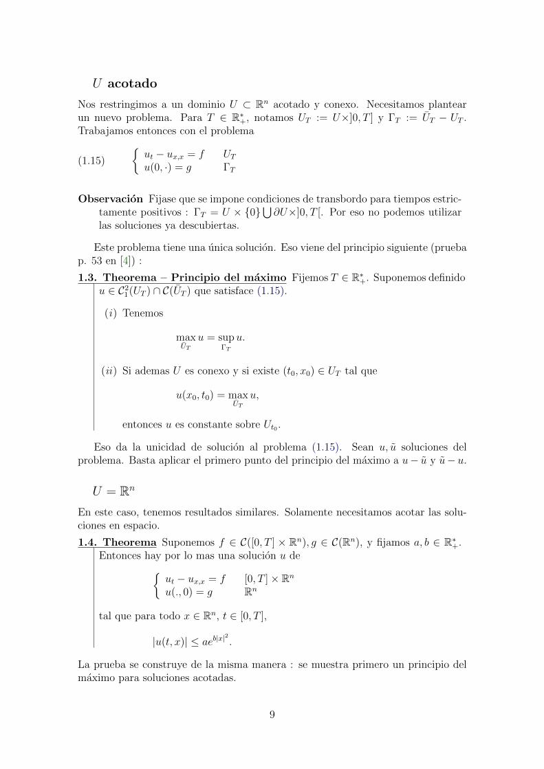
U acotado

Nos restringimos a un dominio U ⊂ Rn acotado y conexo. Necesitamos plantearun nuevo problema. Para T ∈ R∗+, notamos UT := U×]0, T ] y ΓT := UT − UT .Trabajamos entonces con el problema

(1.15)

ut − ux,x = f UTu(0, ·) = g ΓT

Observacion Fijase que se impone condiciones de transbordo para tiempos estric-tamente positivos : ΓT = U × 0

⋃∂U×]0, T [. Por eso no podemos utilizar

las soluciones ya descubiertas.

Este problema tiene una unica solucion. Eso viene del principio siguiente (pruebap. 53 en [4]) :

1.3. Theorema – Principio del maximo Fijemos T ∈ R∗+. Suponemos definidou ∈ C2

1(UT ) ∩ C(UT ) que satisface (1.15).

(i) Tenemos

maxUT

u = supΓT

u.

(ii) Si ademas U es conexo y si existe (t0, x0) ∈ UT tal que

u(x0, t0) = maxUT

u,

entonces u es constante sobre Ut0 .

Eso da la unicidad de solucion al problema (1.15). Sean u, u soluciones delproblema. Basta aplicar el primero punto del principio del maximo a u− u y u− u.

U = Rn

En este caso, tenemos resultados similares. Solamente necesitamos acotar las solu-ciones en espacio.

1.4. Theorema Suponemos f ∈ C([0, T ] × Rn), g ∈ C(Rn), y fijamos a, b ∈ R∗+.Entonces hay por lo mas una solucion u de

ut − ux,x = f [0, T ]× Rn

u(., 0) = g Rn

tal que para todo x ∈ Rn, t ∈ [0, T ],

|u(t, x)| ≤ aeb|x|2

.

La prueba se construye de la misma manera : se muestra primero un principio delmaximo para soluciones acotadas.

9

1.4 Otra ecuacion del calor

Esta ecuacion tiene un efecto regularizante muy fuerte : aun que g sea solamenteC0, la convolucion con φ hace que para todo tiempo t > 0, la solucion es totalmenteregular. Esta regularizacion no es fısicamente aceptable (la informacion viaja conuna velocidad infinita).

Otro fenomeno de transporte es el siguiente. Suponemos que g ≥ 0 y que g noes identicamente nula. Entonces para t > 0, la expresion de φ (1.6) nos asegura enel caso homogeneo que para todo x ∈ U , φ(t, x) > 0. Para ver eso basta elegir unx0 ∈ U tal que g(x0) 6= 0, y por continuidad de g sobre U , existe ε tal que∫

B(x0,ε)

φ(t, x− y)g(y)dy > 0.

Esto vale para todo t > 0, tan pequeno sea. Es decir que la solucion se vuelveinmediatamente no-nula en todo U , aun que g sea nula en algun lugar. Entra encontradiccion con el echo fısico de que la informacion solamente puede propagarse avelocidad finita.

Para obtener un modelo mas realista, se puede cambiar el termino de conduc-tividad ux,x. Para establecer la ecuacion clasica a partir de leyes fısicas, se utiliza laley de Fourier

q(t, x) = −λgrad(T (t, x))

como expresion del flujo de calor, donde λ es una constante. Gurtin y Pipkin – ver[5] – han utilizado otra formula para el flujo de energıa

(1.16) q(t, x) = −T (t, x)γ∫ t

0

K(t− τ)Tx(τ, x)dτ,

donde γ ≥ −1 y K es el nucleo de relajacion. La integral entre 0 y t representa unefecto de memoria. La idea es que el calor no se transmite inmediatamente. Paraconocer la temperatura en x a tiempo t, es entonces necesario saber lo que ha pasadopara los tiempos τ ≤ t (por eso hay una convolucion, una integral) en los puntosdel espacio cercanos de x (por eso se utiliza Tx). Utilizar (1.16) en vez de la ley deFourier lleva a la ecuacion del calor con memoria

(1.17) ut −∂

∂x

∫ t

0

K(t− τ) (T γTx) (τ, x)dτ = 0.

Las soluciones de (1.17) ya no tienen una velocidad infinita para el transporte deinformacion. Si se utiliza para K un dirac 1 y γ = 0, se encuentra la ecuacion delcalor clasica.

1Hay que tomar K = ρε una aproximacion de la unidad, y hacer ε→ 0

10

Chapter 2

Characteristics method

This chapter contains a general result about PDE.We will work on nonlinear first-order PDE. In the general case, we can note the

studied equation as

(2.1) F (Du(x), u(x), x) = 0.

For this we fix in the hole chapter U ⊂ RN open, the set of all x. Then u : U −→ Rrepresent the unknown function and F : RN × R × U −→ R is a function whosevariables will be noted later as p, z, x.

We will also need some boundary condition. We suppose that ∂U is smooth, andwe fix Γ ⊂ ∂U . Then the bondary condition is noted

(2.2) u = g on Γ,

with g : Γ −→ R.We intend to prove here that for x0 ∈ U , there exist V an open neighborhood

of x0, such that our problem is well-posed on V , i.e. has exactly one solution. Wewill suppose for the rest of this chapter that F , which defines our equation, is a C1

function, and that the boundary condition g is a C2 function. If this conditions donot hold, the existence and uniqueness are not guaranteed (see proof of 2.2).

For those who have studied the resolution of transport equation, the idea will besimilar: we try to find curves along which the solutions of our general equation areeasy to compute.

2.1 Changing coordinates

In order to make our problem easier, we will suppose that Γ ⊂ ∂U is flat. We showwe can do this without loss of generality. U is supposed to be C1, hence for x0 ∈ Uwe can find Φ : Rn −→ Rn a C1 bijection that straightens Γ near x0. We supposefor example that Φ(U) ⊂ RN−1 × 0.

Let u be a C1 solution of (2.1), (2.2). We note Ψ := Φ−1, and v := u Ψ, suchthat

(2.3) u = v Φ.

11

By differentiate (2.3), we obtain

Du(x) = Dv(Φ(x)) ·DΦ(x),

and hence (2.1) gives

(2.4) G(Dv(y), v(y), y) := F (Dv(y) ·DΦ(Ψ(y)), v(y),Ψ(y)) = 0,

with y := Φ(x). We finaly note

(2.5) h(y) := g Ψ(y),

and our initial problem has now the formG(Dv(y), v(y), y) = 0 on Φ(U)v = h on Φ(Γ)

with G, h defined by (2.4), (2.5). This new problem is similar to the initial problem,and we can assume for the following that Γ is flat near some special point x0.

2.2 Reduction to an ODE

We first assume that we dispose of u ∈ C2(U,R) a solution of (2.1), in order to finda system of ordinary differential equations (ODE) satisfied by u. We hope this ODEsystem to be easier to solve.

Let’s note x a curve of U :

x :R −→ U ⊂ RN

s 7−→ x(s).

Then we define from this curve

(2.6) z(s) := u(x(s)), p(s) := (Du)(x(s)),

for all s ∈ R. For i ∈ J1, NK, if we differentiate (2.1) with respect to xi, we find withthe chain rule:

(2.7)n∑j=1

∂F

∂pj(Du, u, x)uxjxi +

∂F

∂z(Du, u, x)uxi +

∂F

∂xi(Du, u, x) = 0.

The firsts terms comprise second order derivative which could be complicate to dealwith. But as

(2.8) pi(s) = uxi(x(s)),

we compute

(2.9) pi(s) =n∑j=1

uxjxi(x(s))xj(s).

12

So if we suppose that ∀j ∈ J1, NK

(2.10)∂F

∂pj(p(s), z(s), x(s)) = xj(s),

then we can use (2.9) to get rid of this second order terms in (2.7).We assume for the moment that (2.10) hold, and see what we can deduce. First,

we compute that

z(s) =n∑j=1

uxj(x(s))xj(s),

which gives with (2.8)

(2.11) z(s) = x(s) · p(s).

Then, evaluate (2.7) at x(s) and using (2.9), (2.10) as we said earlier, we obtain

(2.12) pi(s) = −∂F∂z

(p(s), z(s), x(s))pi(s)−∂F

∂xi(p(s), z(s), x(s)).

(2.10), (2.11) and (2.12) are the characteristic equations. If we write them invectorial form, they looks like

(2.13)

(a) x(s) = DpF (p(s), z(s), x(s)),(b) z(s) = DpF (p(s), z(s), x(s)) · p(s),(c) p(s) = −DxF (p(s), z(s), x(s))−DzF (p(s), z(s), x(s))× p(s).

This is a a system of 2N + 1 first order ODE. We can resume what we have doneby

2.1. Theorem – Structure of characteristics equation Let u be a solutionof (2.1). Let s ∈ R 7→ x(s) be a curve of RN . If we define z and p by (2.6),and assume that (p, z, x) satisfies (1.10.a), then (p, z, x) satisfies also (1.10.b)and (1.10.c).

We have successfully obtained an ODE system for any curves of U .

2.3 Conditions on the boundary

In the previous paragraph we toke an arbitrary curve x, and supposed we had asolution u to construct z and p. In the next paragraph we will chose 3-tuples(p, z, x) that satisfy the characteristic equations (2.13) and some initial conditions,and will use them to construct u a local solution of (2.1) (intuitively, we want totake u(x(s)) := z(s), for a well-chosen 3-tuple). Here we talk about this initialconditions.

Let’s take x0 ∈ Γ. We choose a 3-tuple such that x(0) = x0. As we want (2.2)to be satisfied by our future local solution u, we can assume that

(2.14) z(0) = g(x0).

13

What about p = (p1, · · · , pN)? As Γ ⊂ RN−1 × 0 near x0, differentiate (2.2) withrespect to xi (for i ∈ J1, N − 1K) gives

uxi(x0) = gxi(x0).

Hence we can assume that for i ∈ J1, N − 1K, our 3-tuple satisfies

(2.15) pi(0) = gxi(x0).

We obtain an N -th equation for p0 with

(2.16) F (p0, z0, x0) = 0

– where p0 and z0 refer to p(0) and z(0) – as (2.1) must hold at x0.(2.14), (2.15) and (2.16) are the compatibility conditions. A 3-tuple (p, z, x)

with x0 := x(0) ∈ Γ that satisfies them will be qualified as admissible.We want to solve the ODE system near x0, and control its solution with respect

to the initial condition. The following result ensure we can find 3-tuples that areadmissible.

2.2. Theorem – Non-characteristic problem We suppose that

(2.17) FpN (p0, z0, x0) 6= 0,

and that our problem is regular: F is a C1 function, and g is a C2 function.

Then there exist V an open neighborhood of x0, and a unique solution q :V −→ RN of the following problem.

(2.18)

qi(y) = gxi(y) for i ∈ J1, N − 1KF (q(y), g(y), y) = 0

Furthermore, q ∈ C1.

Proof. This result is obtained using the implicit function theorem (see appendixA) to G : RN × RN −→ RN defined for p, y ∈ RN by

Gi(p, y) := pi − gxi(y) i ∈ J1, N − 1K,GN(p, y) := F (p, g(y), y).

G is C1 because of the regularity of F and g ; G(p0, x0) = 0 thanks to compatibilityconditions (2.15) and (2.16) ; finally we have det(DpG(p0, x0)) 6= 0 by calculus:

DpG(p0, x0) =

1 0 0

. . ....

0 1 0Fp1(p0, z0, x0) · · · FpN−1

(p0, z0, x0) FpN (p0, z0, x0)

.

Hence there exist q : V −→ W that satisfies the equivalence given by the implicitfunction theorem. Then for x ∈ V , we haveG(q(x), x) = 0, we are done for existence.For uniqueness, note that the (x, q(x)) are the only couples that can satisfy this lastequality. Suppose we have r a solution of (2.18). Then for x ∈ V , G(r(x), x) = 0and so r(x) = q(x).

14

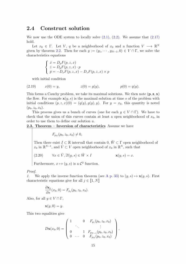
2.4 Construct solution

We now use the ODE system to locally solve (2.1), (2.2). We assume that (2.17)hold.

Let x0 ∈ Γ. Let V , q be a neighborhood of x0 and a function V −→ RN

given by theorem 2.2. Then for each y := (y1, · · · , yN−1, 0) ∈ V ∩ Γ, we solve thecharacteristics equations

x = DpF (p, z, x)z = DpF (p, z, x) · pp = −DxF (p, z, x)−DzF (p, z, x)× p

with initial condition

(2.19) x(0) = y, z(0) = g(y), p(0) = q(y).

This forms a Cauchy problem, we take its maximal solutions. We then note (p, z,x)the flow. For example x(y, s) is the maximal solution at time s of the problem withinitial conditions (p, z, x)(0) = (q(y), g(y), y). For y = x0, this quantity is noted(p0, z0, x0).

This process gives us a bunch of curves (one for each y ∈ V ∩ Γ). We have tocheck that the union of this curves contain at least a open neighborhood of x0, inorder to use them to define our solution u.

2.3. Theorem – Inversion of characteristics Assume we have

FpN (p0, z0, x0) 6= 0,

Then there exist I ⊂ R intervall that contain 0, W ⊂ Γ open neighborhood ofx0 in RN−1, and V ⊂ V open neighborhood of x0 in RN , such that

(2.20) ∀x ∈ V ,∃!(y, s) ∈ W × I x(y, s) = x.

Furthermore, x 7→ (y, s) is a C2 function.

Proof.1. We apply the inverse function theorem (see A p. 33) to (y, s) 7→ x(y, s). Firstcharacteristic equations give for all j ∈ J1, NK

∂xj∂s

(x0, 0) = Fpj(p0, z0, x0).

Also, for all y ∈ V ∩ Γ,

x(y, 0) = y.

This two equalities give

Dx(x0, 0) =

1 0 Fp1(p0, z0, x0)

. . ....

0 1 FpN−1(p0, z0, x0)

0 · · · 0 FpN (p0, z0, x0)

,

15

and so det(Dx(x0, 0)) 6= 0.2. According to the inverse function theorem, it is enough to have regularity onx to obtain the regularity on x 7→ (y, s). Since x is obtained by solving a Cauchyproblem, we are done if we suppose that F is – at least locally – smooth.

From now on we note V := V and W := W the open neighborhoods given bytheorem 2.3. Then for x ∈ V , we define

(2.21) u(x) := z(y, s), p(x) := p(y, s)

where (y, s) is given by 2.20.

2.4. Theorem The function u : V −→ R defined by (2.21) satisfies

F (Du(x), u(x), x) = 0

for x ∈ V , and

u(y) = g(y)

for y ∈ V ∩ Γ.

Proof.1. We begin by the second part of the theorem: let y ∈ V ∩Γ, we show u(y) = g(y).The theorem 2.3 of inversion of characteristics and the definition of u (2.21) ensurethat u(y) = z(y, 0). We conclude by the definition of z (2.19).2. Let y ∈ V ∩ Γ. For s ∈ I – see theorem 2.3 for notations – we define

f(y, s) := F (p(y, s), z(y, s),x(y, s)),

and prove this function is constantly null. Let y ∈ V ∩ Γ. Since p(y, 0) = q(y), and(q(y), z(y), y) is admissible – see (2.16) – we have

(2.22) f(y, 0) = 0.

Furthermore,

fs(y, s) =N∑j=1

pjfpj + zfz +N∑j=1

xjfxj

=N∑j=1

(−fxj − fzpj

)fpj +

(N∑j=1

fpjpj

)fz +

N∑j=1

(fpj)fxj

= 0

The second equality come from the fact that (p, z,x) satisfies (2.13). This calculationand (2.22) show that s 7→ f(y, s) is solution of a Cauchy problem, as well as the nullfunction. Uniqueness of the solution to this problem conclude.3. In 2 we proved – see (2.21) – that for x ∈ V

F (p(x), u(x), x) = 0.

16

To finish up the proof it’s enough to show that for x ∈ V

(2.23) p(x) = Du(x).

For this, we first show

(2.24) zs(y, s) =N∑j=1

pj(y, s)∂xj∂s

(y, s)

for all (y, s) ∈ W × I, and

(2.25) zyi(y, s) =N∑j=1

pj(y, s)∂xj∂yi

(y, s)

for all (y, s) ∈ W × I, and i ∈ J1, N − 1K.The first one of these equalities come from the characteristics equations that

(p, z,x) satisfies. For the second one we fix y ∈ V ∩ Γ. We note, for i ∈ J1, N − 1Kand s ∈ I

(2.26) ri(s) := zyi(y, s)−N∑j=1

pj(y, s)∂xj∂yi

(y, s),

and prove this function is null.Let i ∈ J1, N − 1K. By definition of z,

z(y, 0) = g(y).

Derivating this expression with respect to yi gives zyi(y, 0) = gxi(y). A similarmethod leads to ri(0) = gxi(y) − qi(y). As (q(y), g(y), y) is admissible (q satisfiesproblem (2.18)), this last quantity is null.

On the other hand, for i ∈ J1, N − 1K

(2.27) ri(s) = zyi,s −N∑j=1

(∂pj∂s

∂xj∂yi

+ pj∂2xj∂yi∂s

(y, s)

).

We simplify this expression by differentiating (2.24) with respect to yi:

zs,yi =N∑j=1

[∂pj∂yi

∂xj∂s

+ pj∂2xj∂s∂yi

],

wich gives with (2.27)

ri(s) =N∑j=1

(∂pj∂yi

∂xj∂s− ∂pj

∂s

∂xj∂yi

).

As (p, z,x) satisfies the characteristic equations, we obtain

(2.28) ri(s) =N∑j=1

[∂pj∂yi

Fpj −(−Fxj − pjFz

) ∂xj∂yi

].

17

Finally, differentiate f(y, s) = 0 with respect to yi

N∑j=1

∂pj∂yi

Fpj + zyiFz +N∑j=1

∂xj∂yi

Fxj = 0

and combine it with (2.28) leads to

ri(s) = Fz

(N∑j=1

pj∂xj∂yi− zyi

)= −Fz ri(s).

This, with ri(0) = 0, is a Cauchy problem satisfied by the null function. Henceri = 0, and (2.25) hold.4. Finally, we show that (2.24) and (2.25) implies (2.23). Let k ∈ J1, NK. Thenby definition of u (2.21)

uxk =N−1∑i=1

∂yi∂xk

zyi + sxkzs.

We use (2.25) and (2.24)

uxk =N−1∑i=1

∂yi∂xk

(N∑j=1

pj∂xj∂yi

)+ sxk

(N∑j=1

pj∂xj∂s

),

and we rearrange

uxk =N∑j=1

pj

(N−1∑i=1

∂yi∂xk

∂xj∂yi

+ sxk∂xj∂s

).

We can recognize here – see for example (2.20) –

uxk =N∑j=1

pj∂xj∂xk

=N∑j=1

pjδj,k = pk.

This conclude the proof.

Nota In the special case where our equation is quasilinear, i.e. has the form

N∑j=1

fj(u)uxj = 0,

with fj functions, we can note that (2.13) gives z = 0 and so the solutions weconstruct are constant along the characteristics curves. because of this we donot need the theorem 2.2 (p. 14) and we can use F and g functions that areless regular.

18

Nota In the general case where Γ is not flat, the noncharacteristic condition write

(2.29) DpF (p0, z0, x0) · ν(x0) 6= 0,

where ν(x0) denote a unit normal to Γ at x0.

We can finally sumarize what we have done in this chapter with the followingresult.

2.5. Theorem Let x0 ∈ Γ and W be a neighborhood of x0 such that F ∈ C1, andg ∈ C2 on W . Let (p0, z0) ∈ Rn × R.

If (2.29) hold at (p0, z0, x0), then there exist V ⊂ W open neighborood of x0

such that there exist a unique u solution of (2.1) and (2.2) on V and such thatu(x0) = z0 and ∇u(x0) = p0.

For example the equation

ut + uux = 0

in U := R∗+ × R can be represented by the following application.

F :R2 × R× U −→ R

(p1, p2, z, t, x) 7−→ p1 + zp2

19

Chapter 3

Conservation laws

Here we study a particular equation. Let F : R→ Rn and g : Rn → R be functions.We suppose g ∈ L1. We want to solve the following problem:

(3.1)

ut(t, x) + div(F u)(t, x) = 0 (t, x) ∈ R∗+ × Rn

u(0, x) = g x ∈ Rn

where div denote the divergence with respect to space variable: div(F u) =∑nj=1 Fj(u)xj . The interesting fact about this equation is that the integral of so-

lutions is conserved as the time evolves.Let u be a solution of (3.1). For simplicity we suppose in this paragraph that u

is continuous and has compact support. We note for t ∈ R∗+

I(t) :=

∫Rnu(t, x)dx

and show that for all t ∈ R∗+, I(t) = I(0). We compute that

I ′(t) =

∫Rnut(t, x)dx

= −n∑j=1

∫Rn

(Fj u)xjdx

= −n∑j=1

∫Rn−1

[Fj u]+∞−∞dxj,

where dxj means dx1 · · · dxj−1dxj+1 · · · dxn.As u has compact support, for each j ∈ J1, nK we have [Fj u]+∞−∞ = F (0)−F (0) = 0,and so I ′(t) = 0. This calculus show that the integral of solution doesn’t changewith time. For this reason we call problem (3.1) a conservation law.

In [4] chapter 11 it is studied systems of conservations laws. In this case u :R∗+ × Rn → Rm and F : Rm → Rm×n. This correspond to a system where mphysical quantities are conserved as time evolve, we do not talk about it.

This equations can models fluid flow: for F (u) = uV (u), with u representingthe fluid density and V (u) the fluid speed. It can for example be used to describea traffic flow – though not perfectly, a driver react essentially to what’s happen infront of him, meanwhile a fluid particle is sensible to front and back environment –see [2].

20

3.1 Characteristics method, weak formulation

We want to apply the characteristics method we have exposed earlier. We note

G(q, z, y) = q0 + F ′(z) · p

with y = (t, x), and q = (p0, p) = (p0, p1, · · · , pn). This is the right form to applycharacteristics method. As

DqG(q, z, y) = (1, F ′(z))

and a unit normal to ∂U = 0×Rn is given by (1, 0, · · · , 0), the non characteristiccondition hold and there is a local unique smooth solution to our problem.

Furthermore, DyG = 0 and so characteristics equation ensure that z = 0. Thismean that every smooth solution of a conservation law is constant along the char-acteristics curves.

What about non-regular solutions? If we multiply by v ∈ D(R+ × R) andintegrate, an integration by part gives the weak formulation of this equation(3.1):

(3.2)

∫ +∞

0

∫Rnuvt + f(u) divx vdxdt+

∫Rng(x)v(0, x)dx = 0

Hence we say that u satisfy our problem in the weak sense if (3.2) hold for allv ∈ D(R+ × R).

3.2 Case of dimension one

We begin by interesting ourself to the case n = 1. Then the problem write

(3.3)

ut + f(u)x = 0 R∗+ × Ru(0, ·) = g R

Nota If we take f(x) := 12x2, we obtain the Burger’s equation

ut + uux = 0

we have already see at the end of chapter 2.

In this section we suppose that f is strictly convex.

Rankine-Hugoniot condition

Let suppose we have u a solution that is C1 on V open subset of R∗+ × R, up to acurve γ that goes through V . We assume γ cut V into two distinct regions V− andV+.

21

x

t

VV−

V+

γ

We chose v a test function with compact support in V−. Then the weak formu-lation gives∫

V−

uvt + f(u)vxdxdt = 0

as v vanishes near ∂V . u is then smooth on V− and we can integrate by part∫V−

utv + f(u)xvdxdt = 0.

This equality hold for all v ∈ D(V−), so u satisfy

(3.4) ut + f(u)x = 0 V−.

We obtain the equation on V+ with similar method. Now taking v ∈ D(V ), weobtain from the weak formulation that

0 =

∫V−

uvt + f(u)vxdxdt+

∫V+

uvt + f(u)vxdxdt.

Integrating by part1 and with (3.4), this becomes

(3.5) 0 =

∫γ

[u−n1 + f(u−)n2] vds−∫γ

[u+n1 + f(ur)n2] vds.

Here n = (n1, n2) is the unit normal to γ pointing from V− to V+, and u−(γ(s)) is thelimit of u(t, x) as (t, x) goes to γ(s) and staying in V−. (3.5) hold for all v ∈ D(V ),and so

(3.6) [u− − u+]n1 + [f(u−)− f(u+)]n2 = 0 on γ.

We now make the hypothesis that γ can be write as

γ = (t, h(t)) : t ∈ Wt0(ε),where Wt0(ε) :=]t0−ε, t0 +ε[. We’ll see later that this is not a big restriction. Hence

we have (n1, n2) = α · (−h′, 1), with α = (1 + h′)−12 . Using this expression in (3.6)

finally gives the Rankine-Hugoniot condition

(3.7) f(u−)− f(u+) = h′ (u− − u+) on V ∩ γ.For simplicity, we note from now JuK(t, x) := u−(t, x)−u+(t, x) the jump in u acrossγ at point (t, x). The condition above write

(3.8) Jf uK = σJuK on V ∩ γ,with σ := h′ is the speed of γ.

1See the Gauss-Green theorem p. 33.

22

Riemann’s problem

With the previous paragraph in mind, we try to find solutions of our problem (3.3),in the case where

g(x) :=

u− if x < 0,u+ if x > 0.

x

u−

u+

With this initial condition, we call (3.3) a Riemann problem.First, we uses the characteristics method. We already saw that a solution of a

Riemann problem is constant along the characteristics curves, which are defined by

(3.9) t(s) = 1

and

x(s) = f ′(z(s)) = f ′(z0)

as z is constant along the characteristics curves. Hence

x(t) = tf ′(g(x0)) + x(0).

Note that (3.9) show t(s) = s. This is consistent with the hypothesis we made p. 22on the structure of γ.

Shock

Let suppose first that

u− > u+

As f ′ is increasing we have f ′(u−) > f ′(u+). Then there exist some t ∈ R∗+ for whichtwo characteristics curves will meet, and our solution is no longer smooth. Fromthis time on, we can not use the characteristic method.

x

t

u− = 1.5 u+ = −0.5

The left and right curves will meet, we say there is a shock. We use the Rankine-Hugoniot condition to dicover what happen after this shock. We have a curve ofdiscontinuity – where the shocks takes place – that has to satisfy (3.8). If we take forexample the Burger’s equation – i.e. f(x) := 1

2x2 – with u− = 1.5 and u+ = −0.5,

23

we obtain that Jf(u)K = 1 and JuK = 2. Hence σ = 12

and the shock is the curvegiven by

γ =

(t,t

2

): t ∈ R+

.

This cut U := R+ × R into U− := (t, x) : x < 2t and U+ := (t, x) : x > 2t.Hence we can construct a solution

u(t, x) :=

u− if (t, x) ∈ U−u+ if (t, x) ∈ U+

of Burger’s equation.

x

t

u = 1.5 u = −0.5

γ

Rarefaction wave

We now suppose that

u− < u+,

hence f(u−) < f(u+). In this case, the characteristics curves never cross, the mainproblem here is that there exist point which will never be joined by this curves. Thismean we have to find the correct value of u in this area.

u− = 0.2 u+ = 1

0.2 1?

The first possibility is to choose a solution continuous everywhere – except at (0, 0)– we set for (t, x) in the empty area:

(3.10) u(t, x) = x/t,

which define a continuous solution – called a rarefaction wave – that indeed satisfythe Rankine-Hugoniot condition.

u− = 0.2 u+ = 1

0.2 1x/t

24

But we can also define a non physical shock solution, by setting u = 0.2 inU− := (x, t) : x < αt and u = 1 in (x, t) : x > αt. This define a discontinuitycurve γ defined by (x, t) : x = αt which satisfy the Rankine-Hugoniot condition

for α = f(1)−f(0.2)1−0.2

= 0.6

0.2 1

γ

As this second solution seems non-physical, we would like to find a second con-ditions that the rarefaction wave satisfy, but not this last solution. The problemin the shock is that there is no collision: characteristics curves go away from thediscontinuity. Hence it does not satisfy the entropy condition for a shock withspeed σ:

f ′(u−) > σ > f ′(u+).

As f is supposed strictly convex, this condition becomes u− > u+ at each disconti-nuity.

Other initial conditions

Here we suppose that g ∈ L1 ∩ L∞, and that F is smooth, and F (0) = 0. This lastcondition is not a problem, as F is defined up to a constant.

There is a lot of things we know about solutions in this case. There exist anexpression for weak solutions that uses f ∗ the Legendre transformation2 of f , and(f ′)−1 – which is defined as long as f is strictly convex. It is the Lax-Oleinik formula.

It is also possible to refine the entropy condition, such that we have uniquenessof weak solutions that satisfy the jump condition and this new entropy condition –see [4] p. 150.

The behavior of solution is also known for large t. There is a decay in t−12 of

‖u‖∞, and a limit for ‖·‖L1 . We define, for p, q, d > 0 and σ ∈ R some constants,the N -wave

N(t, x) :=

1d

(xt− σ

)if −

√tpd < x− σt <

√tqd,

0 otherwise.

For well-chosen constants p, q, d, σ – see [4] p. 159 – we have the following result.

3.1. Theorem If g has compact support, the entropy solution u of (3.3) satisfy

2See appendix B.

25

for t ∈ R∗+ ∫R|u(t, x)−N(t, x)| dx ≤ C√

t

for some constant C.

We have numerically check this theorem for simple g. We represent u in function oft and x, see figures 3.1, 3.2 and 3.3.

3.3 Case of dimension two

We now work on the n = 2 case. Here the problem wright

(3.11)

ut + f1(u)x + f2(u)y = 0 on U := R∗+ × R2,u(0, x) = g(x) on R2.

As in the case n = 1, we can establish a Rankine-Hugoniot condition. NowV ⊂ R∗+×R2, and we note S a surface – of dimension 2 – that cut V into two parts.Using the same method as in case n = 1, we obtain an equivalent to identity (3.6):

(3.12) JG(u)K · n = 0 on S,

with G = (idR, f1, f2). As in the previous case, we now suppose that S can be writeas

S = (h(ξ, η), ξ, η) : ξ ∈ Wξ0(ε), η ∈ Wη0(ε) .

Then

v1 = (hξ, 1, 0) and v2 = (hη, 0, 1)

are two tangent vectors to S, hence n is collinear to

v1 ∧ v2 = (1,−hξ,−hη).

With this expression of n, (3.12) becomes

(3.13) JuK = hξJf1(u)K + hηJf2(u)K = ∇h · JF (u)K on S,

with F = (f1, f2).It is also possible to establish an entropy condition, see [8] p. 90.

26

Figure 3.1: Numerical solution of Burger’s equation with g = 1[0,1].

Figure 3.2: The solution goes to a N -wave for large times.

Figure 3.3: Decay in t−12 of ‖u‖∞.

27

Chapter 4

Numerical resolution

We now look at numerically solving the conservation laws. We chose to study the1D Burger’s equation that we have already meet in chapter 3.

4.1 Notations

We begin by fixing the usual notations. We discretize the space by constructing amesh with constant step. For j ∈ Z and n ∈ N, we note

xj := jδx and tn := nδt.

The evaluation of the true solution u is noted

unj := u(tn, xj).

For this particular equation, we will rather use

unj :=1

δx

∫ xj+1

2

xj− 1

2

u(tn, x)dx,

as we already know that integral with respect to space is really stable. We hope thatusing this space average rather than a pointwise evaluation will lead us to betterresults. The computed solution will be write as Un

j , and approximate either unj orunj in function of the used method.

The algorithm is to first construct U0 :=(U0j

)j∈Z by simply taking the initial

condition we have, and then construct Un+1 in function of Un by using the PDE.

Schemes

There is a lot of implicit or explicit method that can be used here, see for example[7] p. 101. We remind here only a few:

? Upwind method: usesUn+1j −Unjδt

andUnj −Unj−1

δxto approximate ut and ux ;

? Downwind method: usesUn+1j −Unjδt

andUnj −Unj−1

δxto approximate ut and ux ;

? Lax-Friedrichs method: uses 1δt

[Un+1j − Unj−1+Unj+1

2

]and 1

2δx

[Unj+1 − Un

j−1

]to

approximate ut and ux.

28

Convergence

We want to know if our computation are useful. We introduce an error function:

E(t, x) = Unj − u(t, x) if (t, x) ∈ [tn, tn+1[×

[xj− 1

2, xj+ 1

2

[.

or:

E(t, x) = Unj − u(t, x)

Remind that this error term depends of δx and δt. We then say that our solutionconverge if ‖E‖L1 → 0 as δt and δx goes to 0.

4.2 Conservative methods

The equation we study is nonlinear, with discontinuous solutions. For those reasons,results like the Lax equivalence theorem – see [7] p. 107 – doesn’t hold, and somemethods will converge – in the above sense – to non solution. For example, let’stake a look at 1D Burger’s equation with upwind scheme. We obtain

Un+1j = Un

j −δtδxUnj

(Unj − Un−1

j

).

If we use

U0j =

1 if j < 0,0 if j ≥ 0.

as initial condition, we can check that for all n ∈ N, we have Un = U0. But this isnot a solution of Burger’s equation, the discontinuity doesn’t satisfy the Rankine-Hugoniot condition.

To prevent this false solutions to appear, we can use method in conservativeform:

(4.1) Un+1j = Un

j −δtδx

[G(Un

j , Unj+1)−G(Un

j−1, Unj )],

with G the numerical flux function. This form comes from the integral formula-tion of the conservation law.1∫ x

j+12

xj− 1

2

u(tn+1, x)dx =

∫ xj+1

2

xj− 1

2

u(tn, x)dx+

∫ tn+1

tn

[u(t, ·)]xj+1

2xj− 1

2dt.

Dividing by δx we obtain

un+1j = unj −

1

δx

∫ tn+1

tn

[f(u)(t, ·)]xj+1

2xj− 1

2dt.

We have obtain (4.1) if G represent the average of the theoretical flux f throughxj+ 1

2, during [tn, tn+1]

G(Unj , U

nj+1) ∼ 1

δt

∫ tn+1

tn

f(u)(xj+ 12, t)dt.

1How to obtain this formulation from the weak one is described in appendix C.

29

Consistency, convergence

We introduce the concepts of consistency. We want to decide if a method is stablelocally. Controlling the whole error can be hard, so we use a local error, defined asfollow. We take u a weak solution of the equation we study, and we compute Un+1

by directly using Unj := u(tn, xj). This way,

L(t, x) =1

δt

[u(t, x)− Un+1

j

]if (t, x) ∈ [tn, tn+1[×

[xj− 1

2, xj+ 1

2

[is the local error corresponding to the method used. Hence we can say this methodis consistent if L(t, x) → 0 as δt, δx go to 0. For conservatives method, we use thefollowing definition of consistency.

Definition – Consistency We say that a conservative method is consistent if

? for all constant function u, the numerical flux equal the theoretical flux

G(u, u) = f(u),

? G is a continuous function of its two variables.

In conservative form, the upwind method becomes

Un+1j = Un

j −δtδx

[(Un

j )2

2−(Un−1j

)2

2

].

Nota This method isn’t always stable, see figure 4.1. In the case of Burger’sequation, it needs that Un

j ≤ 0. If we have Unj , it is more interesting to use the

downwind method. If Unj take both sign, we must alternate the two method,

or change for another one, like the Lax-Friedrichs scheme.

Figure 4.2 show this last scheme, the issues for negative values of Unj have

disappear. The drawback of this method is that it introduce an oscillatingbehavior near discontinuity. For this kind of method, it is interesting to studya convergence in total variation, which also use the ‖·‖1 of ”derivative” of u.

TVt(u) := lim supε→0

1

ε

∫R|u(t, x)− u(t, x− ε)| dx.

More precisely, we say that (Uη)η∈N a sequence of computed solutions converge tothe weak solution u if

? For all K compact of R∗+ × R

‖Uη − u‖L1(K) −→ 0

as η goes to +∞;

? For all T ∈ R∗+, there exist an R > 0 such that for all t ∈ [0, T ] and for allη ∈ N we have

TVt(Uη) < R.

30

Figure 4.1: When upwind method is used, there is numerical issues where Unj ≤ 0.

Figure 4.2: If we rather use the Lax-Friedrichs scheme, this issues disappear. How-ever, an oscillating phenomenon appears near the discontinuity.

31

With this convergence, we have the following result.

4.1. Theorem – Lax-Wendroff We note η ∈ N a grid parameter, such thatδt(η), δx(η)→ 0 as η → +∞. We then note Uη(t, x) the numerical solution ofthe conservation law, computed with a consistent conservative method in theη-th grid.

If (Uη)η converges – in the above sense – to some function u, then u is a weaksolution of the conservation law.

Proof. See [7] p. 131.

32

Appendix

A Various resultsA.1. Theorem – Implicit function Let E, F and G be normed vector spaces.

E × F is a vector space with norm

‖(x, y)‖ := max ‖x‖E , ‖y‖F .

Let U be an open subset of E×F . Let (a, b) ∈ U and f ∈ C1(U,G), such thatf(a, b) = 0 and ∂f

∂y(a, b) be a bijection F −→ G.

Then there exist

? V open neighborood of a in E,

? W open neighborood of b in F such that V ×W ⊂ U ,

? ϕ ∈ C1(V,W ) ;

such that for all (x, y) ∈ E × F ,

(x, y) ∈ V ×W and f(x, y) = 0 iff x ∈ V and ϕ(x) = y.

If furthermore f ∈ Ck(U,G), then ϕ ∈ Ck(V,W ).

A.2. Theorem – Local inversion Lets E,F be Banach spaces, Ω open subsetof E. Let f ∈ C1(Ω, F ), a ∈ Ω such that Df(a) : E −→ F is a bijection. Then,there exist

? V , open neighborhood of a in Ω,

? W , open neighborhood of f(a) in F ,

such that f : V −→ W is bijective and f−1 ∈ C1(W,V ).

If furthermore f ∈ Ck(V,W ), then f−1 ∈ Ck(W,V ).

A.3. Theorem – Gauss-Green Let U be a open bounded subset of Rn, suchthat ∂U is C1. Let u ∈ C1(U), then for i ∈ J1, nK∫

U

uxidx =

∫∂U

unidS,

where ni is the i-th component of a unit outward normal of ∂U .

33

If we apply the Green-Gauss theorem to uv, we obtain an integration by parts formula∫U

uvxidx = −∫U

uxivdx+

∫∂U

uvnidS.

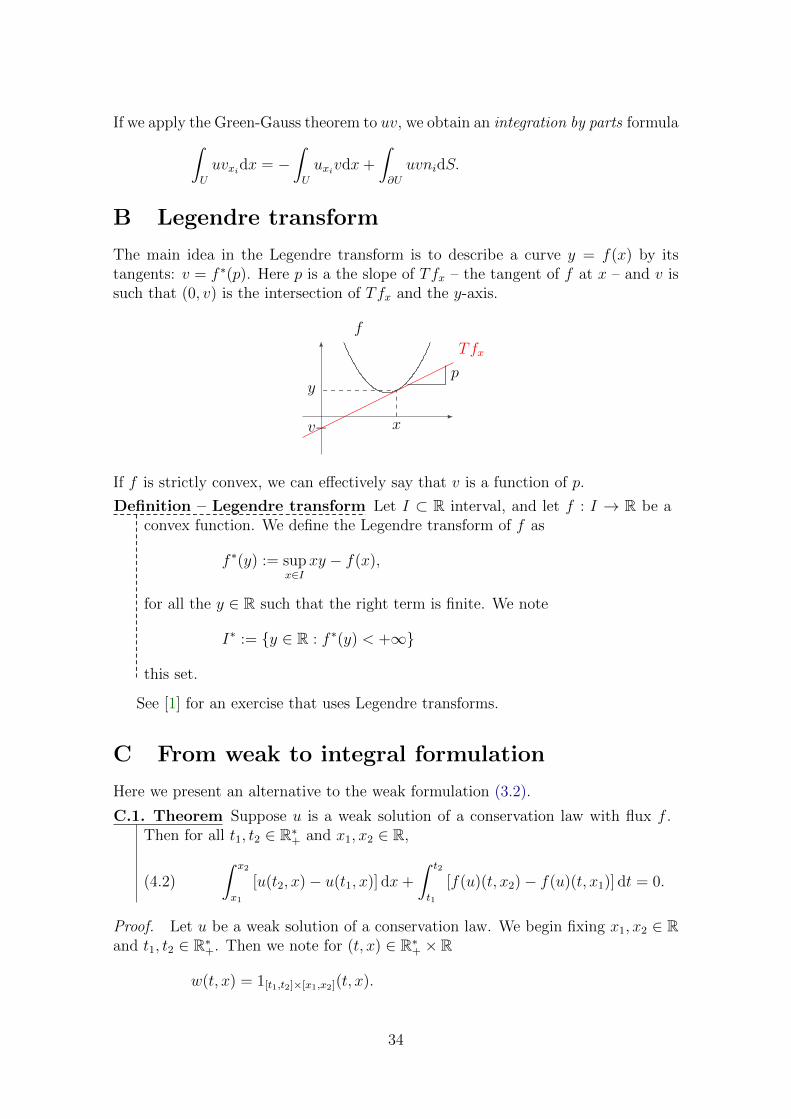
B Legendre transform

The main idea in the Legendre transform is to describe a curve y = f(x) by itstangents: v = f ∗(p). Here p is a the slope of Tfx – the tangent of f at x – and v issuch that (0, v) is the intersection of Tfx and the y-axis.

f

Tfx

x

y

−v

p

If f is strictly convex, we can effectively say that v is a function of p.

Definition – Legendre transform Let I ⊂ R interval, and let f : I → R be aconvex function. We define the Legendre transform of f as

f ∗(y) := supx∈I

xy − f(x),

for all the y ∈ R such that the right term is finite. We note

I∗ := y ∈ R : f ∗(y) < +∞

this set.

See [1] for an exercise that uses Legendre transforms.

C From weak to integral formulation

Here we present an alternative to the weak formulation (3.2).

C.1. Theorem Suppose u is a weak solution of a conservation law with flux f .Then for all t1, t2 ∈ R∗+ and x1, x2 ∈ R,

(4.2)

∫ x2

x1

[u(t2, x)− u(t1, x)] dx+

∫ t2

t1

[f(u)(t, x2)− f(u)(t, x1)] dt = 0.

Proof. Let u be a weak solution of a conservation law. We begin fixing x1, x2 ∈ Rand t1, t2 ∈ R∗+. Then we note for (t, x) ∈ R∗+ × R

w(t, x) = 1[t1,t2]×[x1,x2](t, x).

34

Then for ε ∈ R∗+, we note wε = w ? ρε, with (ρε)ε a unity approximation. Thenwε ∈ D, and we have

(4.3)

∫ +∞

0

∫Ru∂twε + f(u)∂xwεdxdt+

∫Rg(x)wε(0, x)dx = 0.

As ε goes to 0, the second integral goes to 0 because t1, t2 > 0. Furthermore,

∂twε = (∂tρε) ? w

−→ε→0 δt0w.

where δt is the derivative of the Dirac distribution. Hence∫R∗+×R

u∂twεdxdt −→∫ x2

x1

[u(·, x)]t2t1dx.

We do the same with the second part of the first integral to conclude.

35

Bibliography

[1] http://perso.eleves.ens-rennes.fr/~lgare802/documents/oral_

concours_3a_corentin.pdf, 2017.

[2] A. Aw and M. Rascle. Resurrection of ”second order” models of traffic flow.Feb-Mar 2000.

[3] J. M. Burger. A mathematical model illustrating the theory of turbulence – Ad-vances in applied mechanics, Vol 1. 1948.

[4] Lawrence C. Evans. Partial Differential Equations. American MathematicalSociety, 1997.

[5] Pietro H. Harris and Roberto Garra. Nonlinear heat conduction equations withmemory: Physical meaning and analytical results. May 2016.

[6] Frederic Lagoutiere. Equation aux derivees partielles et leurs approximations.

[7] Randall J. LeVeque. Numerical method for conservation laws. Birkauser, 1992.

[8] Yuxi Zheng. System of conservation laws, Two-dimensional Riemann problem.Springer science+Business media, LLC, 2001.

36