AN ANNU L LfCATION VOLU ME 14 - 15 /1 985 -1986

HACEllEPE BUllETl1i Df

NATURAl SCIIICIS AND IIGINIIRI

A BULLETIN PUBLISHED BY HACETTEPE UNIVERSITY, FACULTY OF SCIENCE

H\CETTEPF III UETIN OF NATUR.\L SClEi\:CES AND E!,;GI1'EI:I{\;\(;

AN ANNU,\1~ PL'I3L1CATION VOLUME 14-15;1985-19H6

SAH1BI OWNER

Hacetrepe Oniversitesi On Behalf of Hacerrepe

Fen Fakultes i Adina Uru ver s it v Faculty of Science

OKYAY ALPAUT

EDtTOR EDITOR

AYSE BOSGELMEZ

YAYIN KURULU OYELERi EDITORIAL BOARD

LAWRENCE M. BROWN

SONER GONEN

KAzlM GONER

A~KIN TOMER

TEKN1K ED1TOR TECHNICAL EDITOR

FAHRETTtN SAVCI

A BULLETIN PUBLISHED BY HACETTEPE UNIVERSIlY, FACULTY OF SCIENCE

OverseasTurkeySubscription Rate (Yurt DI~d( Yur tici )(Abone Bedeti) S 8.004000 TL.

Address for Correspondenc\: (Yazrsma Adresi)

HACETTEPE ONIVERSITESI FEN FAKOLTESI

BEYTEPE. ANKARA 06532 TORKiYE

PRINTED AT THE FACULTY PRESS (FAKULTE MATBAASINDA BASILMl~TIR)

@ 1986

CONTENTS

C. Clrakoglu, G. omurtay, M. Ankan Application of Microcarr i e rs

to a Rabbit Kidney Cell

Line 1-6

M. I. Khanfar Modular Representations

of PSL(2,7) in Character­

istics 3 and 7 7-14

M. Kutkut. On the Class of Paranormal

Operators 15-24

M. Kutkut Ergodicity of Hiltert

Space Operator s 25-33

O. AltInta~

On the Coefficients cf Certair

Meromorphic Functions ..... 35-40

A. YIlmaz

A Characterization of

Units in 2S4...•..•. : ....•41-52

H. E~

P Ncte on Fuzzy Nearly

Compact Spaces 53-59

A. Hannanci Matrix Baer*-Rings 61-67

A. Harmanci Some Remarks on the

Commutativity cf Rings .... 69-75

iCINDEKiLER

C. Clrakoglu, G. omurtay, M. Ankan MH,rota~lYlcllarln Tavsar

Bbbregi Daimi HOcte KOltOrOne

L'ygulanmasl i-6

M. I. Khanfar PSL(2,7)'nln Karakteristik

3 ve 7 i~in Modular

Tems i Ici Ie r i 7-1a

M. Kutkut Paranormal Oper sto- ler

Slnlfl Hakklnda 15-24

M. Kutkut Hilbert Uzay OperatOr­

l er i nin Erqodik l i9i 25-32

O. AltInta~

Bazl Meromorf Fonksiyonlarln

Katsayllarl 35-40

A. YIlmaz

ZS4'On Birimselleririn

bir Karakterizasyonu 41-52

H. E~

Belirtisiz Topolojik Uzay­

larda vek m Trk i z l ik ......52.·:.9

A. HarmanCI Matds Bae'*-Halkalar 1 •••• 61-67

A. Harmanci Halkalar In KomOtati f1 iginde

Bazl Katklla t 69-75

H. TatlIdil Power Comparisons of Some Out! ier

Tests 77-90

E. E. SOzer, M. Sucu Partial Solution for

Stackelbelg Disequilibl ium in Duopoly 91-99

C. Erdemir, S. Cak.mak A Dynamic Regression Analysis

of the Energy Consumption

BasE:e or. Income 101-108

Editorial Board . Preperation of Final Typescript

-Applied and Experimental

Sciences- 109-112

Editorial Board Preperation of Final Typescript

-Mathematics and Theoretical Statistics- 113-116

H. Tat l rdi l

Baz 1 Ayk 1 I 1 Deger Testlerinin Etkinliklelini~

Ka'~1Ia~tlrllmasl 77-S0

E. E. Sozer, M. Sucu iki Satlclll Piyasada

Stackelberg Dengesizli£i DUlumunda Klsmi ~ozOm ..... 91-99

C. Erdemir, S. Cakmak Gel i Ie Dayanan Enerj i TOketiminin Dina~ik

Regresycn ~nalizi 'O'-'C8

Yaytn Kurulu

Yaz i n1n Son Sek lin in Hall rl art 1~ 1

-UY9ulamal1 ve Deneysel

Bilimler- 109-112

YaYln Kurulu Yazi run Son Sek l i ni n Haz i r-l arus i -Matematik ve Teorik istatistik- 113-116

SERIES A

BIOLOGY

Hacettepe Bulletin of Natu~al Sciences and rnginee~ing

1985/ Volu.e 14/pp. 1-6

APPLICATION OF MICROCARRIERS TO

A RABBIT KIDNEY CELL LINE

k -1 (1) G (2) M Arlkan(2) C. Clra og u , • Omurtay , .

Microcarriers (Cytodex 1) were applied to a rabbit kid­ney (RK) cell line.

We found that 1 mg/ml Cytodexl was optimal for growth of rabbit kidney cells. Rabbit kidney cells were subculte­red every seven days when they were grown as a monolayer in glass culture bottles. On the other hand RK cells grown on microcarriers were subcultered every fifteen days. Cyto­dex beads provide a large surface area for the cells and therefore cells grown on Cytodex 1 maintain excellent grow­th kinetics over long periods.

We conclude that microcarrier cultures are more econo­mical than the ordinary monolayer cultures.

Key words: Microcarriers, Cytodex I, Cell line

INTRODUCTION

Microcarriers are a new idea in cell culture techniques pionee­

red by van Wezel [7].

In microcarl'ier cell culture; cell s prol iferate as a monola­

yer on small posHive(y charced beads of sephadex which are sus­

pended in a medium contained in culture bottles [3] .

The large surface to volume ratio offered by the microcarrier

system results in high yields of anchorage derendentceTIs(oftenas

high as 5xl06 cells/ml with 3-5 mg microcarriers/ml) [1].

(1) Hacettepe Urrive r sj.ty , Faculty. of Science, Department of Biology , Ankara,T~RKEY

(2) Hacettepe Universi~y, Sc~oo} of Medidne, Medical B'io l oav Department, Ankara ,TURKEY

2

More than 80 different cell tYres have been reported to orow successfuly on Cytodex 1 microcarriers [2] .

Cytodex 1 microcarriers are based on a cross-linked dextran matrix which is substituted with positively charqerl N,N-diethyl aminoethyl (DEAE) groups to a denree which is optimal for cell

growth. The charged grours are found throughout the entire matrix of the microcarrier (Fig.1).

In this study we tried to arow a rabbit kidney cell line on

Cytodex 1. This cell line grew perfectly on it.

Also we established the microcarrier culture method in our laboratory. So we can try to arow other kinds of cells, par t tcu­

larly transformed ones by this method.

MATERIALS AND METHODS

I. CELLS AND MEDIA

The rabbit kidney cell line was obtained from World Health

Organization (WHO) Geneva, Switzerland. RK cells were grown in Eaole's minimal essential medium (MEM)

supplemented with 10 % newborn calf serum and antibiotics.

II. PREPARING CYTODEX 1 FOR CULTURE

Cytodex 1 was obtained from Pharmacia Fine Chemicals, Upsala,

Sweden. The dry Cytodex 1 microcarriers (1 mg/ml) were added to a glass bottle and were swo l l en in Ca++, t1q++ free PBS (50-100

ml/qr Cytodex) for at least 3 hours at room temnarature with occa­sional agitation [6J. The sunernatant was decanted and the mic­

rocarriers were washed once with gentle aaitation for a few minu­. ++ ++tes ln fresh Ca , Mq free PBS.

After swell ina the microcarriers in Ca++, ~g++ free PBS, they

were allowed to settle, the supernatant being decanted and repla­

ced by 70 % (v/v) ethanol in distilled water.

3

The microcarriers were washed with this ethanol solution and then

incubated over~ight in70 % (v/v) ethanol (50-100 ml/gr Cytodex)

for sterilization. The ethanol solution was remowed and the steri ­lized microcarriers rinsed three times in sterile Ca++, Mg++ free

PBS and once in culture medium before use. Sterilized microcar­riers were resuspended in a small volume of culture medium and

transferred to the glass petri dish.

III. INITIATING A MICROCARRIER CULTURE

Rabbit kidney cells were put on the petri dish containing

Cytodex 1 and 30 ml MEM supplem@nted with 10 % serum was added to

the culture. Microcarrier culture was incubated at 370C with

occasional agitation.

IV. HARVESTING CELLS AND SUBCULTERING

The medium was drained from the culture and the microcarriers washed for 5 minutes in a Ca++: Mg++ free PBS solution containing

D.02 % (w/v) EOTA,pH 7.6. The amount of EOTA PBS solution should

be 50-100 ml/9r Cytodex. The EOTA PBS was remowed and replaced

by trypsin-EOTA at 37 0C with occasional aaitation.

After 15 minutes the action of tryrsin was stopped by the addi­

tion of a culture medium containing 10 % (v/v) serum.

The products of the harvestina stens were then transferred to a

test tube. After 5 minutes the microcarriers settle to the bottom

of the tube and the cells can then be collected in the SUDer­

natant.

RESULTS

Rabbit kidney cells attached themselve~ to the microcarriers

3 hours after the cells were put ", Cv t nnex 1. Rf; cells ClrevJ we l l 10 hours af tei s t.a r t i no the 1I1l( lUI"I! 1('1' ,ul LUI'e.

Cells ~rown on beads of Cytodex 1 maintained excellent qrowth

4

kinetics over long periods (Fig.2). We changed the culture me­

dium with MEM containinq 3 serum a week after the microcarrier

cul ture started.

Culture orown on Cytodex 1 were more homogeneous than monola­

yer and harvesting was achieved without centrifuging the medium.

Cylodex ,

Charges

1hroughoul 1he matrix

FIGURE 1. Schematic Representation of the Charged Grours

on the Cytodex 1 Ricrocarrier

16.0

lI'l

0 4.0 )(

E- 1.0 ~ QI u

0.25

0 100 200 300

Hours

FIGURE 2. ~e Growth of RK Cells on Cytodex 1 Microcarriers

and in Glass Bottles as Monolayer

5

DISCUSSION

We applied a microcarrier culture method to rabbit kindey cell line. Cells easily adapted to cytodex beads. Cytvdex beads provide a large and smooth surface for the cells

to attach on [5] . We modified some of the stages of the microcarrier culture

method. We did not stir the suspension culture [4J , because the magnetic stir bar can cause collision of the beads. Collision of beads was harmful for cells. Also stirrino causes the detac­hing of mitotic cells from the beads. We therefore put 30 ml of medium in petri dishes containing the microcarrier culture of RK cells. The occasional aoitation on the petri dishes was enough to keep this kind of suspension culture healthy. The optimal concentration of Cytodex 1 beads was 1 mg/ml for RK cells. When the concentration of Cytodex 1 was high, they preci­pitated at the bottom of the petri dish, and they stuck to each other. But when the Cytodex r concentration was decreased to 1 mg/ml, an ideal culture condition was obtained. The microcarrier culture method we used in this study is more economic than the monolayer culture, since we used a low serum concentration in maintaining the culture medium, e.g. 3 % serum supplemented MEM was used in the microcarrier culture, while 5 %

serum supplemented MEM was used in the monolayer culture. Also RK cells in the microcarrier culture were subcultured only every 15 days, w~'er.eas RK cells in the monolayer culture were subcultured every 7 days. We can say that Cytodex 1 saves up to 50 % of our labour becaus~

it is no longer necessary to process large numbers of petri dis­hes or culture bottles.

We plan to try to grow some of the poorly growing transfor­med cells on microcarriers.

,. ;

6

OZET

Tavsan b~bre~i daimi hUcre k~tUrUne mikrotaS1Y1Cllar (Cytodex 1) uygulandl. Tavsan bobreni daimi hUcre kUltUrUne opti ­

mal uremesi icin mikrotaSlylcl konsantrasyonunun 1 mg/ml Cytodex 1 oldugu saptandl.

KUltUr siselerinde monolayer olarak Uretilen RK hUcreleri her 7 gUnde bir pasaj yaplldlol halde, mikrotaS1Ylcllarda Uretilen RK hUcreleri 15 gUnde bir pasaj yaplldl.

Cytodex bilyeler hUcreler l~ln genis yUzey sa91adlolndan Cytodex 1 Uzerinde Ureyen RK hUcreleri uzun zaman periyodunda sagllkll Ureme kinetini qosterdiler.

MikrotaS1Ylcl kUltUrlerin monolayer kUltUrlerden daha ekonomik olduau soylenebilir.

REFERENCES

1. Clark, J.M. and Hirtenstein, M.D. Optimizing culture conditi ­ons for the production of animal cells in microcarrier culture. Annals.N.Y. Acad. Sci. 369, 33-46, 1981.

2. Clark, J.M. and Hirstein, M.D. AmerIcan Tissue Culture Assn. 31s Annual Meeting. St. Louis. Abstract 96, 1980.

3. Grinnel, F., Hays, D.G. and Winter, D. Cell adhesion and spreading factor partial purification and properties. Exp, Cell. Res. lID, 175-190,1977.

4. Ham, R.G. and He Keehan, W.L. Media and growth requirements Methods in Enzymo]opy 58, 44-93, 1979.

5. Maroduas, N.G. Adhesion and spreading of cells on charged surfaces. J. Theor. BioI. 49, 417-424, 1975.

6. Pharmacia Fine Chemicals Microcarrier cell culture. Technical Booklet Series. 1981.

7. van Wezel, A.L. Growth of cell strains and primary cells 1n homogeneolls culture. Nature 216, 64-65, 1967.

SERIES B

MATHEMATICS AND

STATISTICS

7 Hacettepe Bulletin of Natural Sciences and Engineering

1985/ Volu.e l'/pp. 7-1'

MODULAR REPRESENTATIONS OF PSL(2,7)

IN CHARACTERISTICS 3 and 7. *

M. I. Khanfar (l)

In [6], the ordinary representations of the unimodular group G = PSL(2,7) of dimensions 3,6,7 and 8 were explicitly constructed over the complex field. The aim of this work is to investigate the modular representations of G over finite fields. This paper determines the irreducible modular repre­sentations of G in characteristics 3 and 7.

Key words: Modular representation, Characteristic, Decompo­sition matrix, Blocks.

1980 Subject Classlflcation: 20C20

(. INTRODUCTI ON

Most of modular representation theory is due to R. Brauer. His

results were stated in the language of modular charac­

ters in ( [I] , [2] ).

1.1.DEFINITION. Let G be a finite group and p a rational prime. An

element g in G is p - regular if its order is relatively prime to

p, and p - singular if its order is a power of p.

Sinceall conjagateelements inGareof the same order,.' we speak

of the p - regular conjugacy classes of G.

The following two established results ([3 ],[7 I) will be applied

wi thout further ret erence ,

-----_.-------- ._- -- . .. - -- _. - ._-- ' ..

(1 Matl:«ti :", 1)'>1'\., i-..itlif f".l"lUj,\ZJZ iiIl1'/., .Jeudan , SAUDI ARABIA.

* This work wa~ suppcirted by a grant t'rom Yarmouk University.

8

(l) The number of absolutely irreducible modular representations

of G in a modular field of characteristic p is equal to the number

of p - regular conjugacy classes of G.

(2) Let e oe an absolutely ir-reduc ib l e ordinary representation

of G. If pm is the highest power of p dividing the order of G and

the degree of ~,then ~ remains absolutely irreducible as a modular

representation of G in characteristic p.

The following proposition is needed and can be applied in any

characteristic p t 2.

1.2. PROPGSITlON. Let K be an algebraically closed field of charac­

teristic pt2. Then G = PSL(2,P) has no faithful representation of

deqree 2 in K [7]

Proof. Let f G -->GL(2,K) be a monomorphism. Then

det : f(G) ---~K* is a homomorphism onto a finite subgroup of K*.

All such subgroups of K* are cyclic.

If p>3, then f(G), being 'simple, is a subgroup of SL(2,K).

If p=3, then G=A4 and so at least det (f(G)) ~{l,-l}.

Choose an involution x in G such that f(x) is in SL(2,K). Putting

f(x) in rational canonical form. we find that f(x) is similar to

l ' and therefore f (x) = But then th i s

• -I.L 'J implies that f(x) is in the center of the simple group f(G); a

contradiction.

2. REPRESENTATrONS IN BLOCKS

Wp cons i der a metnod of d i-.; iIHI:'U\C] the rspresenta t i ons ot a

fl:II:P qruu:.,G i nt o b l ock s I 1'3) 141, [5J). Let K be an algeb­

ra ic number t ield which IS d S[.J11 LLillg field for' G, and R the !'in\] of algebraic integers in K. Let S be d prIne ideal in R containing

- -

- -

- -

9

the unique rat i onal prime p. Let R be the ring of S - integrals elements in K. Then R is a principal ideal ring with quotients field K; and R=R/ = R/ is a ~odular field of characteristic p

R s s ( [1] , [3] , [4] ). Theory of integral representations of finite

groups asserts that, every irreducible representation of Gover K

can be written as an integral represent.at i on of Gover R ' s -

Let Ci be the sum of the elements in the conjugacy class Ci of

G, i = I, ... , n. Let e , be all Irreduc i ble integral representa­1 _

tions of G, and xi the character' of t i . The sums Ci form a K-basis

for the center of the group ring KG as well as a K-basis for the

center of KG. !hus each Ck commutes wi th each gin G, and therefore

the matr i x e, (Ck) commutes with the matr-Ix e. (g) for each LSchur's1 _ 1

Lemma asserts that each t i (C is a scalar matrix; that isk)

(*) t i (Ck) = f i (C k) I, I < k < n .

-Since t i is an integral representation, we have each fi(C k) is in

R ' Taking traces in (*), we haves

- ICkl xi (gk)fi(C k ) = . <i k<n

xi (l)

Extending f to a map on the center of KG by linearity, we havei

f i (Cj Ck) = f i (C j) f i (Ck) .

We define Ti center (KG) ------~K by

f i (Ck) = f i (Ck) , i < k < n

Whel'e the bar denotes reduction modulo S. Two irreducible repre­

sentations t · and t of G be lonq t o [he same block iff T = T . 1 J I J

If t belongs to a block B, t her .r l ! !IJP\lilcjl,lt-> modu l er cons t i­i tuents of e . belong necessuri ly tu l50

1

, Ie

2.1. DEFINITION. Let p be a rational prime, n a rational integer. We write v (n) e if pe divides nand pe+l does not divide n.p Assume v (IGI) m.p 2.2. DEFINITION. The defect d of a p - block B is given by

d = m - mi n {vp ( xi (l)) : ~ i in B} •

Clearly each d?O. A P - block of defect 0 contains only one ir ­reducible representation ~i whose degree is di visible by pm [I].

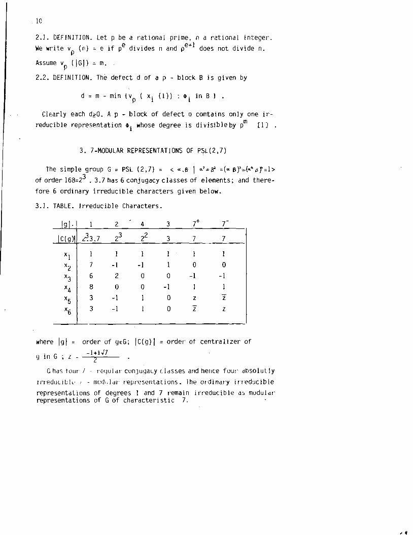
3. 7-MODULAR REPRESENTATIONS OF PSL(2,7)

1 =The simple group G = PSL (2,7) = < «.8 I 0. 13:< =(<< ar:,,.(Q.4~j:l>

of order 168=23 .3.7 has 6 conjugacy classes of elements; and there­fore 6 ordinary irreducible characters given below.

3.1. TABLE.

Igl·

IC( g)l

Xl x2 x3 x4 Xs x6

Irreducible Characters.

I 2 .

4 3 +7 7 ­

~3.7 23 22 3 7 7

I 1 1 1 I 1

7 -I -1 1 0 0

6 2 a 0 -1 -1

8 a a -1 I 1

3 -I 1 0 z z 3 -1 I a z z

where Igi = order of gEG; IC(9)1 = order of centralizer of -1+i ../7

g in G ; z 2.---- ­0: - ......

Ghas tour' 1 l'eLjuldl' conjuqat.y c lasses and hence four' absolut ly

trredui.Iul« j - modular represent.at i ons • 1he ordinary irreduc ib le

representations of degrees I and 7 remain i r reducib Ie as modu lar representations of G of characteristic 7.

.. t

11

By Proposition 1.2 the two ordinary irreducible representations

of degree 3 are irreducible as modular representations of

G in characteristic 7; but of course these representations are

equivalent in this characteristic.

To determine the fourth irreducible 7 - modular representation

of G, we detemine first the blocks of the ordinary irreducible

representations of Gand the defects of these blocks. To distribute

these representations into 7 - blocks, we form the table:

21 42 56 24 24

7 -4 -4

- -7 3 3 f i (Ck) = -7 14 46 46

-7 14 46 46

-3 -6 8

o=-1+iJ7.

Reducing the table modulo a prime ideal containing 7, we obtain:

3 3

3 3 3 3

3 3

3 3

-3

Thus there are two 7-blocks:

B {I,3,3,6,8,} of defect I, andI=

{7} of defect 0;B2=

where the representations in each block are indicated by their

degrees. If n is the degree of the unkown irreducible 7 - modular

12

representation of G, then 1,3, n are in B The possible valuesi. for n are 4,5,6,8 . Since B is of defect I, each entry in theI decomposition matrix D associated with B is either 0 or 1([2],[3] )l 1 It follows that the only possible value for n is 5 and 01 has the

form:

mod. deg. 5 3

ord. deg. 1

6

8 1

3 1 3 1

Hence the decomposition matrix D of G is of the form:

= I 1] .D2

In fact the ordinary 6 - dimensional representation of G obtained

in [6] , when reduced in characteristic 7, fixes the hyperplane

<ej - e l > • If we restrict to this hyperplane,

then with respect to the"basis {e - e ' j = 2, .••. 6 } j l

we obtain:

2 1 1 1 --1 -1 -1 -1 -I ­

I 2 I 1 1 cr __> 1 1 2 I 'a->

1 I I 2

1 1 I I

4. 3- MODULAR REPRESENTATIONS OF PSL(2,7)

G = PSL(2,7) has five 3 - regular' conjugacy classes of elements,

..

13

and hence five irreducible 3 - modular representations. The ordinary

irreducible representations of Gof degrees 1,3,3,6 remain absolutely

irreducible as modular representations of G in characteristic 3.

Following the methods of the preceding section, we find that the

ordinary irreducible representations of G are distributed into four

3 - blocks:

Bl = { 1,7,8 } of defect 1,

and B = {3} , B = {3} , B4 = {6} of defect 0;2 3

where the representations in blocks are indicated by their degrees.

Let the unknown irreducible modular representation of G be of

degree n, Then n is in B The possible values for n are then 4,5,l• 7,8. Since B is of defect I, each entry in the decomposition matrixl 01 associated with Bl is either 0 or 1. It follows that the only

possible value for n is 7; and thus D is constructed as follows~l

mod. deg. 7

ord. deg. 1

7

8

Hence the decomposition matrix 0 of G is of the form:

o -02

o = o

where 0i [1], i=2,3,4.

aZET

Karma~lk saYllar cismi Ozerinde boyutlarl 3,6,1 ve 8 olmak u­

14

zere bir G=PSL(2,7) unimcdul ar qrubunun adi temsi l Iert yapr lmi st i r [6]. Bu ~a11~manln amaCl, sonlu cisim1er Ozerindeki G grubunun mo­dLirer temsillerini arast i rmakt u-. Bu arest irma 3 ve 7 karakt.er-t s­tikleri i~in G nin indirgenemeyen temsi11erini be1ir1er.

REFERENCES

1. Brauer, R. and Nesbitt, C. On the Modular Characters of Groups, Ann. of Math. 42,556 - 590, 1941.

2. Brauer, R. Investigations on Group characters, Ann. of Math, 42, 936-958, 1941.

3 . Curtis, C. and Reiner, 1. Representation Theory of Finite Groups and Associative Algebras, Wiley-Interscience, N.Y., 1962.

4 . Dornhoff, L" Group Representation Theory Part B, Marcel Dekker, Inc. N.Y. lY72.

'5 • feit, W. Representations of Fini te Groups 1. Notes, Yale Univer­sity, 1909.

6 . Khanf'ar , M. Complex Representations of PSL (2,7), Hacet.t.e pe Bull. of Natural Sc i , and Eng.,l3, 69-79, 1984.

7 . Serre, J. -P. Linear Representations of Finite Groups, Springer - Verlag, N.Y. Inc., 1977.

15 Hacettepe Bulletin of Natural Sciences and Engineering

1985/ Volu.e l~/pp. 15-2~

ON THE CLASS OF PARANORMAL OPERATORS

~.Kutkut (1)

In this article we study some properties of the class of paranormal operators on an infinite dimensional separable complex Hilbert space H. We prove the following.

1. The tensor product and the direct sum of two paranormal operators are paranormal.

2. The set of paranormal operators is strongly (uniformly) closed and arcwise connected.

3. Every paranormal weighted shift is hyponormal.

4. If T is a paranormal weighted shift on H then Pn(T) is paranormal on H(but P (T) may not be hy ponor-mal ) . for any

npolynomial P .

n Key words: Paranormal operators, weighted shift, Hy~onor­mal operator.

1980 Subject ClassIfIcation: 47B20

1. INTRODUCTION

We consider an infinite dimensional separable complex Hilbert

space H. We denote by L(H), all bounded linear operators on H. As

in [1] , an operator T E L(H) is said to be paranonnal if IITxl12s

IIT2xll, for all unit vectors XE H, ( or equivalently

IITx!IZs 11TZxll.llxll, for' every xEH). Recall that an operator

hL(H) is said to be hyponorme l , if IITx Ii ~I rr'~x II, for' every x £ H

(or equivalently T*T,:T T"'). An uperdtl'~ 1 LL(H) is called nonnaloid

(1) MathematICS Uept.,King Abdulazlz UnIV., Jeddah, SAUDi ARABIA.

16

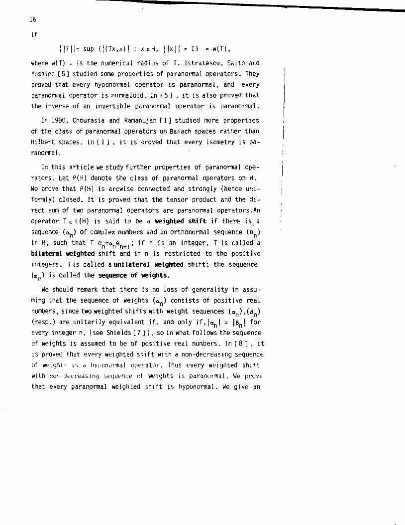
4

if

I/TI/= sup {1(Tx,x)1 : XEH, IIxll = 1} = w(T),

where w(T) = is the numerical radius of T. Istratescu, Saito and Yoshino [5] studied some properties of paranormal operators. They proved that every hyponormal operator is paranormal, and every paranormal operator is normaloid. In [5] , it is also proved that the inverse of an invertible paranormal operator is paranormal.

In 1980, Chaurasia and Ramanujan [I] studied more properties of the class of paranormal operators on Banach spaces rather than Hilbert spaces. In [I] , it is proved that every isometry is pa­ranormal.

In this article we study further properties of paranormal ope­rators. Let P(H) denote the class of paranormal operators on H. We prove that P(H) is arcwise connected and strongly (hence uni­formly) closed. It is proved that the tensor product and the di­rect sum of two paranormal operators are paranormal operators.An operator T E: L(H) is said to be a weighted shift if there is a

e.

sequence (~n) of complex numbers and an orthonormal sequence (en) in H, such that T en=~nen+l; if n is. an integer, T is called a bilateral weighted shift and if n is restricted to the positive integers, Tis called a unilateral weighted shift; the sequence (an) is called the sequence of weights.

We should remark that there Is no loss of generality in assu­ming that the sequence of weights (~n) consists of positive real numbers, since two weighted shifts with weight sequences (~n) ,(Bn) (resp.) are unitarily equivalent if, and only if,l~nl = IBnl for every integer n, (see Sh ie Ids [7 ] ), so in what fa 11 ows the sequence of weights is assumed to be of positive real numbers. In [8], it IS proved that every weighted shift with a non-decreasing sequence of weight:, 1" d hYJ'llnUI1TldI upel'dtl11·. Thus every weighted srurt with Ilufl-ueUed"ITlQ "elluence ut weIghts is pe renorme l . We [wove that every paranormal weighted shift is hyponormal. We gi ve an

17

example of ~ paranormal operator which is not hyponormal. Shields [7] asked whether Pn(T) is a hyponorma l operator for a hyponormal unilateral weighted shift T and every polynomial P . In 1984, Pengn . Fan [6] gave a negative answer to Shield's question; he construc­ted a hyponormal unilateral weighted shift T for which Pn(T) is not hyponormalfor a given polynomial Pn. Here we prove that Pn(T) is a paranormal operator for a paranormal weighted shift T and any polynomial P In fact t(T) is a paranormal operator for a pa­n. ranormal weighted shift T and any function t, which is analytic on the spectrum otT) of T.

Z. RESULTS

To be precise let HI~ HZ denote the completion of the tensor product of the two Hilbert spaces HI and HZ. If Te:L(H I), Se:L(HZ) then the tensor product TiS of T and S belongs to L(H I i HZ). Con­cerning the tensor product we prove the following.

2.1. PROPOSITION. If T,S are paranormal operators on HI,HZ(resp), then TiS is paranormal.

Proof. If x,y are unit vectors, then x ~ y is a unit vector and we have

l! ' i S xi y lIZ = IITxIlZ. IIsyllZ 5 IITZxll.IISZyll

511 T2 i sZ x i y II= II (T is)z x i y" ,

which implies the conclusion of the proposition.

2.2. PROPOSITION. If TE L(H I), S E: L(HZ) are paranormal, then the direct sum T ~ SE: L(H I i HZ) is paranormal.

Proof. If x = Xl ~ Xz is a unit vector in HI i HZ then,

liT ia SX" Z "I iT xI liZ + lIS XzliZ ~ . . 2

':: 111 ( x J I I • 1 I x I 1\ -+ lis xzll . 11 Xz II ~

" .,e

18

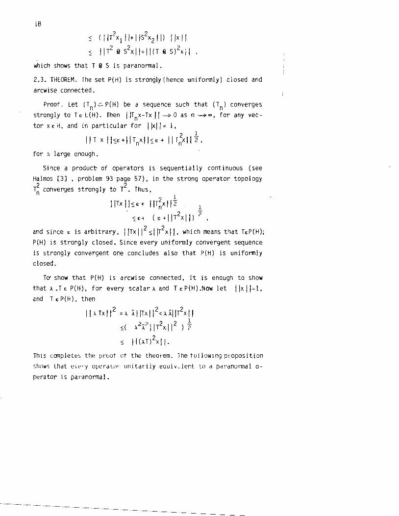
s: (IIT2xI 1/+ Ils2x2 II) !Ix II

IITz6aSzxll=IHT6aS)zxll,~

which shows that T ~ S is paranormal.

2.3. THEOREM. The set P(H) is strongly (hence uniformly) closed and

arcwise connected.

Proof. Let (Tn)C.P(H) be a sequence such that (Tn) converges

strongly to TE: L(H). Then IITnx-Tx II ~ 0 as n ~"', for any vec­

tor x £ H, and in particular for Ilxll = I, 2 1

II T x II ~E: +IITnX II~ E: + II TnX II "2 , for n large enough.

Si nce a product- of operators is sequent i a lly cant i nuous (see

Halmos [3] , problem 93 page 57), in the strong operator topology

T~ converges strongly to T2• Thus,

l/Tx 11-:;£+ IIT2x l l"2

1 1n

'S e + (£ + IIT2xII) "2 and since e is arbitrary, IITxllZs11T2xll, which means that hP(H);

P(H) is strongly closed. Since every uniformly convergent sequence

is strongly convergent one concludes also that P(H) is uniformly

closed.

TCY show that P(H) is arcwise connected, it is enough to show

that A.TE: P(H), for every scalar A and T£P(H).Now let IIxll=l,

and T£P(H), then

II ATx 11 2 =A ~ IITx liZ < A~lIT2x II $( A2~211T2xl ,Z ) ~

s 11(;~,T)2xll.

This conp le tes the uroot ot the theorem, The t nl l owi no propcs i t ion

shows that eVf:"y ope ra tor uni t ari ly equiv ..lent to a perenornat o­

perator is paranormal.

19

2.4. PROPOSITION. Let TE P(H), then for any unitary operator u on

H, uTu*EP(H).

Proof. If TEP(H). u is a unitary operator on H, then for a unit

vector x EH, we have x = uy for some unit vector y E H. and 2

II uTu*xl1 2 =IITu*xI1 = IITyl12 2u*xl I~IIT2YII =1 IT

-::lluT2u*x 11 sl !(uTU* )2x 11,

which is as desired.

2.5. PROPOSITION. If T. SE P(H). S is an isometry which commutes

with T, then TSEP(H).

Proof. If x is a unit vector in H, S is an isometr~ then y=Sx

is a unit vector and one obtains 2 2 2y

IITSx 11 = I/Ty 11 < IIT II

-:: IIT2Sxli 2Sxl I= I IST

-::1~(TS)2xl"

since S commutes with T, i.e., TS is paranormal.

The following proposition is concerned with the integral powers

of a paranormal operator.

2.6. PROPOSITION. Let TE P(H), then for every positive integer n,

TnE p(H) .

Proof. If T is paranormal then it is norrnaloid (see [5] ) which

is equivalent to saying IlTnxll = llTx lin, for every positive inte­

ger n, sincellTxlf-:: I\T2xll for any unit vector XE H, one conclu­

des that IITnxl1 2 2)n<IIT2xll n

= (I\TxI1

IIT2nxii < = II(Tn)2 x l l .

which means that Tn is paranormal.

20

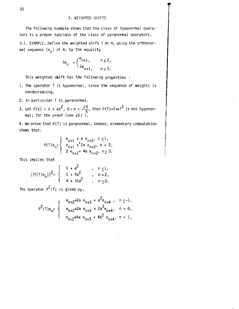
3. WEIGHTED SHIFTS

The following example shows that the class of hyponormal opera­tors is a proper subclass of the class of paranormal operators.

3.1. EXAMPLE. Define the weighted shift T on H, using the orthonor­mal sequence (en) of H, by the equality

Ten ={en+ l• n $ 2, 2en+l , n <: 3 •

This weighted siift has the following properties

1. The operator T is hyponormal, since the sequence of weights is nondecreasing.

2. In particular T is paranormal.

3. Let P(z) = z + ai, 0 < a < v';, then p(T)=T+aT2 is not hyponor­mal; for the proof (see [6J ).

4. We prove that PIT) is paranormal. Indeed, elementary computation shows that:

e +l + a e +2 , n ~l,n ne +l +#2a e +2, n = 2,n n2 e +1+ 4a e +2, n» 3. n n

This impl i es that

f +i n-;:l, 2=IIP(T) e I1 1 1 + 4a2 n =2,n

4 + 16i n >3.

The operator p2( T) is given by,

2 en+3 + a en+4 ' n -;: -I,en+2+2a

2p2(T)en~ { en+2+2a en+3 + 2a en+4, n = 0,

en en+3 + 4a 2 n = I,+2+4a en+4,

21

From which we conclude,

2 4+ 4a + a , n 'S-1 ,

i + 4a2 + 4a4 n 0,

2(T)e 2 2+ 4IIP 11 = + 16a 16a n 1,n

4 + 64a2+ 64a4 , n = 2,

2 416+ (16) 2i + (16) a , n e 3.

4By comparing the value of IIp(T)e 11 and IIP2(T)enI12 one concludes n thatllp(T)enll2 ::;lIp2(T)eril ' which is as desired.

3.2. REMARK. The restriction on a to be such that 0 < a < 4 is

needed in [ 6] to show that P(T) is not hyponorma1 but it is not

needed to show that P(T) is paranormal.

3.3. EXAMPLE. Let T be the weighted shift defined on (en) by

i , n <0en+ l T(e = n) {

, n? O.en+l

It is clear that T is hyponormal and therefore it is paranormal.

Hartman [4] showed that the spectrum o(T) of T is not a spectral

set of 1. Recall that ~ subset X of the complex plane is said to

be a spectral set of T if 0 (T) C X and for any rational function

,twith poles off X we havell«T)II<~~~I~(Z) I (=II~IICXl)'

This example shows also that it is not necessary for the spectrum

of a paranormal operator to be a spectral set.

The following proposition shows that every paranormal weighted

shift must be hyponormal.

3.4. PROPOSITION. If T is a paranormal weighted shift, then its

22

sequence of weights (an) satisfies the inequality

Proof. If (en) is the orthonormal sequence on which T is defi­

ned, then liTenl12 = a~, and IlT2en II=an.an+1 and since T is para­2normal then a <a.a I'n - n n+

Example 3.1(4) is not only true for P{z) :: z + ai but it is true for any polynomial. This is shown in the following.

3.5. THEOREM. Let TEP{H) be a weighted shift, Let P(z) be a poly­nomial of degree k. Then P{T) is a paranormal operator.

Proof. Let (en) be an orthonormal sequence in H, (an) the weight sequence. If T defined by Ten =anen+ l is paranormal then an.:.an'~+l

for every integer n. If P(z) is a polynomial of degree k, i ,e .• P(z): l+alz + a2i + + akzk, ai complex numbers, i::1,2 •...•k, then an elementary computation s~ows that,

IIP{T)enI12:: 1 +lalI2a~ + la212a~+1 +•.• + lakI2a~.1i+l"~~+k

and 2{T) 2

I IP e l 1 :: I + 41al 12a~ +12a2 + al al 12 a~.a~+l + '" +n

+1 akl2 a~.a~+l •.•a~+2k·

By comparing IIp{T)e 114 and IlpZ(T)enIIZ one concludes thatn IIp{T)e liZ :.11 pZ{T)enll. for every integer n, which shows that n P{T) is paranormal as desired.

3.6. THEOREM. Let TEP{H) be a weighted shift. 1ft is any analytic function on the spectrum o(T) of T. then t{T) E P{H).

Proof. Since t is an analytic function then there is a sequenCE of polynomials (Pk) which converges uniformly to~. By Theorem 3.! Pk(T) is paranormal for every k, By Theorem 2.3 the unifonn l i mit t(T) = u-lim Pk(T) is paranormal.

23

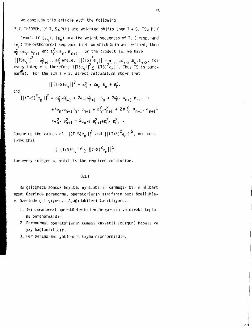
We conclude this article with the following

3.7. THEOREM. If T, Se:P(H) are weighted shifts then T + S, TS£ P(Hl.

Proof. If (~n)' (Bn) are the weight sequences of T, S resp; and (en) the orthonormal sequence in H, on which both are defined, then

~~ '::'~n· ~n+l and B~'::'~n' Bn+l· For the product TS, we have

IITsen,, 2 = a~+l . B~ while, II(TS)Ze l l = an+l.an+3.Bn.Bn+Z' fornevery integer n, therefore IITSe liZ< IPS) Ze II. Thus TS is para­

, n - n normal. For the sum T + S, direct calculation shows that

and

IlfT+S)2en I f ~ a~.a~+l + 2an·a~+1· Bn + 2a~. an+1 Bn+ l +

Comparing the values of II(T+~)en If and II(T+S)2en I f, one conc­ludes that

for every integer n, which is the required conclusion.

OZET

Bu cal i snada sonsuz boyutlu ayr-i.l ebi l i r karmas ik bir H Hilbert uzayl uzerinde paranormal operatorlerin Slnlflnln bazl ozellikle­ri Ozerinde c;all~lyoruz. A~agldakileri kanltllyoruz.

1. lki paranormal operatorlerin tensor carp inn ve direkt topla­ml paranormaldir.

2. Paranormal operator-Ier in kUmesi kuvvetli (dUzgOn) kapel i ve yay baQlantllldlf.

3. Her paranormal yOklenml~ kayma hiponormaldir.

24

4. T,H uzer inde paranormal yuk l enrni s kayma ise bu duromde , her

P polinomu i~in Pn(T),H (izerinde paranormaldir (ama hipo­n normal olmayabilir).

REFERENCES

1. Chaurasia N. and Ramanujan P.B. Paranormal operators on Banach spaces, Bull. Austral. Math. Soc. Vol. 21, 161-168, 1980.

2. Douglas R.G. Banach algebra techniques in operator theory. A­cad. Press N.Y. 1972.

3. Halmos P.R. A Hilbert space problem book. Van Nostrand 1967.

4. Hartman J.A hyponormal weighted shift whose spectrum is not a spectral set. J. Operator Theory. 8, 401-403, 1983.

5. Istratescu V.,Saito T &rl YOShino T. On a class of operators. Tohoku Math. Journ. Vol. 18, no. 4, 410-413, 1966.

6. Peng Fan. A note on hyponormal weighted shifts. Proceedings of the Amer. Math. soc. Vol. 92, no. 2, 271-272, 1984.

7. Shields A.L. Weighted shift operators and analytic function theory, Math. Surveys, no. 13, Math. Soc. Providence R.I. 1914.

8. Stampfli J.G. Which weighted shifts are subnormal. Pacific J. of Math. vol. 11, no. 2, 367-318, 1966.

25 Hacettepe Bulletin of latural Sciences and [ngineering

19851 Volu.e l\/pP' 25-}}

ERGODICITY OF HILBERT SPACE OPERATORS

M. Kutkut (1)

In this article the following theorem is proved. Theorem: If T is an ergodic operator (in the uniform, strong or weak operator topology) on an infinite dimensional complex Hilbert space and F is a continuous multiplicative function then F(T) is ergodic (in the respective tooology). Th t e result implies that S T S-~ is er~ndic for any invertible operator S : the adjo Lnt, 'f*of 'f is ergodic. If T is subnor­mal then the minimal normal extension N of T is ergodic. Moreover the dual S of a pure subnormal operator T is ergodic.

Key words: H~lbert space, Mult~pl~cative function, Ergod~c

operator

1980 Subject Class~f~cation: 47A35

I. I NTRODUCTl ON

Let X be a Banach space, and L(X) the algebra of all bounded

linear operators on X. totz in [3] introduced" the following defi­

nition of ergodicity.

1.1. DEFINITION. Let GcL(X) be a multiplicative semi-group of opera­

tors. Denote by chG the convex hu11 of G. Then Gis sai d to be

ergodic if the closure of chG has a zero element, i.e., there exists

a projection operator P in the closure of chG such that PS = SP=P

for every operator'S in the c Iosure of chG. If the closure of ch G

" is taken in the uniform operator topology then G i s called uniforwly ergodic and if the closure of chG i s t aken In till-' str onq operator

(t\, ~H&theinatl.cs Dept. I King Abdu Iaz rz Univ., Jeddah, SAUDI ARABIA.

26

operator topology then G is called strongly ergodic. If the underlying

space is an inner product space then weakly ergodic may be simi larly

defined. Denote these closures of chG by uchG, schG and wchG res­

pecti vely.

1.2. DEFINITION. Let TEL(X), then T is said to be ergodic (in the

unifonn, strong, or weak topology (for inner product space)) if the

cyclic semigroup GltTn: n::O ,1,2, ... } is ergodic in the respec­

tive topology.

2. RESULTS

In this paper we study ergodicity of operators on Hilbert space.

If H is an infinite dimensional complex Hilbert space, L(H) deno­

tes the algebra of all bounded linear operators on H.

Let U be the unitary group on H. The unitary orbit U(T) of TeL(H)

is defined by

U(T)= {u T u* : u EU, u* :: adjoint of u l •

The similarity orbit S(T) of TeL(H) is defined by

S(T) :: ( s T S-l: 5 is invertible L

Now, we are ready to introduce our results.

2.1. LEMMA. If F is a 1-1 mul t ip l l cat Ive function, and TeL(H), such

that F(T)eL(H) , then F induces a multipl icati ve function F between

GT and GF(T)' which is one to-one and onto.

Proof. Define F : GT -->GF(T)' by

F(Tn) .= Fn (T).

It is an easy matter to show that F is multiplicative, one-to­

one and onto.

2.2. REMARK. F t 0, I , P : P is a prcj ect ion,

2.3. LEMMA. The multiplicative function F defined in Lemma 2.1 is

27

extendable to a multiplicative function denoted by F (for simplicity) between ChGT and ch GF(T)' which is also one-to-one and onto.

Proof. If AECh GT then there exist positive integers nl'··n~ nk and non-negative real numbers al, •.. ,ak:~i ai = 1 and A=~i aiT 1

n . n. Now the extension of F is defined by F(A) = ~,aiF(T 1)=~, aiF I(T).

m. 1 1

If BECh GT then B = 3b T J, for some positive integers ml, ••. ,mj l and some non-negative real numbers bl, •.• ,b l whose sum is one, and

ni +mjthus AB= f rai bj T , and since i 7j aibj = 1,AB EChGT that is, chGT is a semi-group (See Lotz [3] .p , 146). The function F is multiplicative, since

n.+m. F(AB) = .z. a.b . F(T 1 J)

1 ,J 1 J n. m.

. z . aI'b . F(T 1) F(T J)1 , J J

n. m. = z a. F(T 1)) ( 4 b . F(T J))

i 1 J J

= F(A).F(B).

It is not difficult to show that F is one-to-one and onto.

2.4. LEMMA. If the multiplicative function F is continuous, then the function Fdefined in Lemma 2.3 is extendable to a multiplicative function (denoted by F) between the closure of ch GT and the closure

of ch GF(T)' which is also on~-to-one, onto and continuous.

Proof: In the um torm.rtopoloqy, if AE uch GT, then there is (Ai)cCh GT such that IIA:"Aill ~>O as i _>CD. Since F is con­tinuous and multiplicative ChGF(T) and F(chGT) can be identified. By continuity of F, F(A i) converges uniformly to F(A) and we can define F: uch GT -----;>uch GF(T) by F(A) = u-lim. F(A i) , where u-Itm, means uniform limit. From the definition of F, it is clear that F is continuous on uchGT. Since F is one-to-one in Lemma2.3then by linearity, F is one-to­

28 r one on uch GT. If B f: ucn GF(T) , then there is a sequence (B i) -cn GF(T) such that (B i) converges uniformly to B. Since BiECh GF(T)'

then there is Ai Ech GT such that Bi = F(A i) (because F is onto by

lemma 2.3).Since F is continuous and one-to-one, it is invertible

and thus (Ai) converges uniformly to AEuch GT, so that by the de­

finition of F, F(A) = B or F is onto.

If A,B Euch GT then A=u-lim. Ai,B=u-lim Bi for(Ai),(Bi)cChG T"

Since multiplication is continuous (and in particular sequentially

continuous) in the uni form topology( see Halmos[ 2] , probl em 91,page

57) we have, AB=u-lim AiB This implies that~i•

F(A B)= u-lim F(AiB i) = u-lim F(A i). F (Bi)

= u-lim F(Ai)u-lim F(Bi) = F(A) F(B),

since F is multiplieative on ch GT by Lemma 2.3. Thus F is multip­

licative on uch GT.

For the strong topology, a s'imi lar argument can be gi ven, since the

product is sequentially continuous in the strong operator topology

(see Halmos [2] , problem 93 page 57).

Since the product is not even sequentially continuous in the weak

operator topology, (see Halmos[ 2], problem 93 page 57) we provide

the following argument to show that the extension F:wch GT ~wch

GF(T) is mUltiplicative.

It is known that if Ai -;> A weakly then AiB ~AB, BA i -"BA weakly

for any fixed operator B(see Halmos [2] problem 92 page 57).

If A Ewch GT and B Ech GT' then there is (Ai) in ch GT such that

(Ai) -.;. A, weakly and thus (AiB) -;:>AB weakly, as i -,,<Xl; and by

the continuity of F, (by the definition of F in the weak operator

topology), and since F is multiplicative on ch GT,

F(A B)=w-lim F(AiB)= w-lim F(A i ) F(B)

=F(A). F(B), (2.1)

29

wher'e w-lim means weak-limit.

Now, assume that both A, BEwch GT, then there ext st (B i) in en GT: B=w-l im Bi. Therefore AB i ~ AB weak ly as i ---7 ex> and AB Ech GT• this implies that (by continuity of F in the weak topology):

F(AB) = w-lim F(A.B i) = w-lim F(A).F(Bi),by (2.1)

= F(A) .F(B) •

i.e., F is multiplicative on wch ~T.

2.5. THEOREM. Let TE L(H) be an ergodic (in the uniform, strong or weak operator topology) operator, then for a 1-1 continuous multip­licative function F, for which F(T) E L(H), F(T) is ergodic.

Proof. By Lemma 2.4, F induces a continuous mu lt i pl icati ve function denoted by F, (for simplicity) which is one-to-one and onto between

the closure of ch GT and the closure of ChGF(T)' (in the uniform, strong, or weak operator topology). If P is a zero element of the closure of ch GT then F(P) is a zero element of the closure of ch

GF(T)' (in the respective topology). Indeed, since P is a zero e­lement, then PS = SP = P, for every S in the closure of ch GT. If

A is an element in the closure of ch GF(T) there is S in the clo­sure of ch GT such that A= F(S), since F is one-to-one and onto. Since F is also multiplicative one obtains,

F{P).A=F{P).f{S)=F{P.S)=F(P) =F.{S.P) = F(S). F{P) =A.F(P).

This implies that F{T) is ergodic.

We prove the following results as corollaries of the Theorem.

We should remark that the term ergodic is understood in the three topologies unless otherwise mentioned.

2.6. COROLLARY. Let TE L(H) be ergodic. If S is an invertible ope­rator on H, then ST S-1 is ergodic.

30

Proof. Define F:GT ~G -1 by F(Tn): S TnS-l• It is clear' that STS

F is I-I, mUltiplicative and continuous (for any fixed operator S,

see Halmos (2] problem 92). It is' also one-to-one and onto. By the

Theorem F(T) : S T S-I is ergodic.

2.7. REMARK. Corollary 2.6. means that if T is ergodic then every

element in the similarity orbit S(T) of T is ergodic.

2.8. REMARK. Since every unl t ary operator u is invertible and u-l=u*,

the adjoint of u, it follows from Corollary 2.0, that u T u*is er'­

godic and thus, every element of the unitary orbit U(T) is ergodic.

2.9. COROLLARY. If T £ L(H) is ergodic then the adjoint T* of T is

ergodic. n

Proof. Define F: G -:>GT*by F(Tn):T* which is a multiplicativeT isometry (one-to-one) and onto. Moreover, F is continuous (in the

unifonn and weak topology but not in the strong,see Halmos [2 ] problem

90 page 56). By the Theorem F(T) = T* is ergodic (in the uniform

and weak operator topologies).

Since, uch GT* c sch GT * C wch GT * , one concludes that schGT*has

a zero element, i.e.T* is strongly ergodic.

2.IO.COROLLARY. If T £ L(H) is ergodic, then F(T) is ergodic, for

every analytic multiplicative function F, on the spectrum a(T) of T.

Proof. It is not difficult to show that a multipl ication analytic

function is one-to-one, onto, and continuous. (see lenati< 2.11).By

the Theorem,· F(T) is ergodic.

2.11. REMARK. If F(z) is analytic, where z is a complex variable,

then

F(z)= ~ anzll and F(z) F(z) = F(z2), thus

( I a zn)(Ia zn) = Ia z2n o non 0 n

I for some n and this is true if a = and thus F(Z)=Zn.{ ' n J otherwi se

31

2.12. REMARK. Corollary 2.:C:and the preced i nq remark imply that if

T is ergodic then r'' is ergodic tor every positive integer nand

thus every element in the cyclic semi-group GT is ergodic.

For a subnormal operator T, let N be the minimal nonnal exten­

sion of T (which is unique up to unitary equivalence, see Halmos

[2], problem ISS, page 101). Conway [1] showed that N can be writ­

ten as a two-by-two matri x with oper-ator entries.

N= [~ where NE L(K), N is normal and Kis a Hilbert space such that K=HiH I • If the decomposition K=HliH is considered then the adjoint N*of N

is given by

A*l T*J

The operator T is said to -be pure subnormal if T is subnormal

and neither A nor Tis norma 1. 011 n( [4] Lemma 5.3) has observed

that T is pure subnormal if, and only if, N*is the minimal normal

extension of S, and S is called the dual of T.

2.13. COROLLARY. Let T EL(H) be an ergodic subnormal operator. If

N is the (unique) minimal extension of T, then N is ergodic.

Proof. If f is an analytic function, then it is proved in Conway

Il l that f(N) is the minimal normal extension of f(T). Using the

decomposition mentioned above,

f (T) F(N)= 0[

where N is defined on H i HI.

In part Icu lar let f be multipl icaUve and ana.lytic endsc, b;Y'~r*-i;'

. 2.11, f(z)= zn, for some n.DE!fine themulttplicdti~e·\'C06t:·,

funetion r. Gr ~ ~~f(~~"oi~eti"i,"J"d .....

32

the minimal normal extens ion of Tn, F is one-to-one and onto. By

the theorem. N=F(T) is ergodic.

2.14. REMARK. SInce N is unique, by symmetry the proof of Corollary

2.13 implies that if N is ergodic then T is also.

Finally, we arrive at the following result concerning the dual of

a pure subnormal operator.

2.15. COROLLARY. If hL(H) is a pure subnormal operator, and if S

is the dual of T, then T is ergodic if and only if S is ergodic.

Proof. Let N be the minimal normal extension of T, then (by O­

lin's result (4] ) the adjoint tf is the minimal normal extension

of the dual S of T if, and only if, T is pure. Thus if T is ergo­

dic then by corollary 2.13, N is also ergodic. By Corollary 2.9 N*

is ergodic, and by Remark 2.14, S is ergodic. By the symmetry of

the proof we have if S is ergodic then T is ergodic too.

bZET

Bu \all~mada a~agidaki teorem kanltlanml~tlr.

TEOREM. T, bir sonsuz boyutlu karma~lk Hilbert uzaYI uzerinde

(duzgun, kuvvetli veya zaylf operator topolojisine gore), bir er­

godik operator ve F carp imsa l surek l i bir fonksiyon ise ayru topo­

lojiye gore F(T) ergodiktir. Boy lece herhangi b i r terslenebilir S

operet.oru i c i n STS- 1 ergodiktir; T nin T*eki ergodiktir. T alt nor>

mal ise T nin minimal normal qeni s Iemesi N erqod i kt i r , Ostelik, bir

pur alt normal T 0peratorunun S duali ergodiktir.

REFERENCES

'",nWil'. 'lhe dual o r a subnormal ope r-a t.o r , Journal o t "i'd'arOI' '" lI'Y \i,'J, 110.;', PI':>-2ll, l':J8i.

iLdIIIJ:.: , i! i I bed, s pa c '"'! pm book, I)'HI Nostrand N. 'l .l9f"t .

3. L.otz, H.P. Un i for-rn e r-god i.o th.,,,ren,;J for r"br"wv Operators on C(Xi.

33

Mathematisch p Z~itschrift If8,145-156-Springer-Verlag 19B1.

4. Olin, H,.. ,~ncLional reldtionships between a subnormal ope­rator and ~ts minimal normal extension, Pacific J. Math., 63 221-229, 1976.

35 Hacettepe Bulletin of latural Sciences and Engineering

1985/ Vol..e l'/pp. 35-'0

ON THE COEFFICIENTS OF CERTAIN MEROMORPHIC FUNTIONS

The aim of this work is to obtain the sharp bounds for the coefficients of the functions belonging to the class of meromorphic functions which are analytic in o<lzl<l. Key words: Analytic function, function of order a .

Meromorphic function, Starlike

1980 Subject Classification: 30030

1. INTRODUCTION

An analytic function 1 2g(z)=-+b 1Z+b2z +... z

is said to be starlike of ordera ,(O~a<1) in the punctured disc

K={z:o<lz\ <1} if and only if Re {-zg'(z) }>a

g(z)

for all z in the unit disc E={z: IZ1<1}. Let F be the cl ass of, functions u

1 2f (z)= -z- + a1z-e2z +...

which are analytic in K and satify the condition

zfl(z)zf'(z) +1 1<1 u ( -1,I (0~ 0::;1) .z E E .•• ( 1. 1 ) g(z) 9 z)

(1) Hacettepe Univ.,Fac. of Sci., Hath. Dept., Ankara, TURKEY.

36

where 1 2g(z)= --z-- + b z+b2z +...

is analytic and starlike of order ~ in K. Owa[3J has obtained some coefficient relations for the class Fu

taking 00 n

f(z)=z+ n~2anz

analytic in the unit disc E,

g(z)=z- 'f b z" , (bn~O)n=2 n

analytic and starlike of order o i n E.

A special subclass of Fu was studied by Kaczmarkski [1].

Pommerenke [4] has obtained the relation

Ibnl~ 2(1-0.) n=1,2,... . (1.2)n+1

for the meromorphic function 1 _ 2g(z)= -Z + ...+b 1z+b2z

which is starlike of order 0. in K.

In this paper, using this result we obtain the coefficients re­

lation for the class Fu '

2. RESULT

2.1. THEOREM. If f(z)EF u and Re akbk~o for k=1,2,3, ... (n-2) then

2(1-0.)n I an k1+u+ ,n~1 •

n+1 The bounds are sharp.

Zf I (z) -1 J ... (2.1)g(z)

+•.• and Iw(z)! <1 in E. On substituting the

f(z), g(z) and w(z) in (2.1) we have

37

1+u -- +Z

kI1 [-(1+U)+ k~1 (u k a (2.2)(ka k+bk)zk+1= k-bk)l+1]W(z)...

Equating coefficients of z2 and z3 on both sides of (2.2)

we get

and

~ -(1+u)C2a2+b2 3"

Using IC21~1, IC31~1 and from (1.2) we obtain

I a 11~la 1+b11 + I b11 ~ 1+u+1- ~ ... (2.3)

and 2(1-~)

... (2.4)3

Equating the coefficients of zn (n>2) on both sides of (2.2) we get

... -t u(n-2)a _ ] C •. :(2.5)n 2-bn_2 2

-. From (2.2) and (2.5) we obtain

n-2 . .k+1. kCD..

:[ -(1+u)+ k~1 (u k ak-bk)z ] w(z) + k~n+2 dkz .•• (2.6)

CD CD •k+1 k Since k~n+1 (kak+bk)z = k~n+2 [(k-1 )a k_ 1-bk_1] z

dnd 1rom (2.6) we have

(2.7).

38

Us i ngIw(z ) 1<1 in E and Parseval identi ty(L2J,p: 100) on both sides

of (2.7) we obtfin

n I ' 2 2(k 1) 2 . r < (1+u)2 +k~1 kak+bk ; . r + + k~n+2 jekl 2k

. •. (2.8)

If we let r --->1, from (2.8) we have

n 2· 2 n-2 k~1 !kak+bkl ~(1+u) + k~1 I uk ak-bkl 2 •.• (2.9)

or

2 - j(n-1)a _ _ 1 •.• (2.10)n 1+bn 1

Since o~u~1 and Re ak5 ~ 0 (k=1 ,2, •.• (n-2) it follows thatk

nan+bn 1~ 1+u •.. (2.11)

From (1.2) and (2.11) we have

nlanklnan+bnl +Ibnl-:S 1+u+ 2~:;a) , n=3,4,5, ...... (2.12)

Hence from (2.3), (2.4) and (2.12) we obtain

n ja 1<1+u+ _2..U~) for n=1 ,2,3, .•. n ..... n+1

Now let us show that the bounds are sharp.

We take zf I (z ) _(1+z n+1)

= g(z) 1_uzn+1

and 2 ( 1-0.)

, 1)q(z) (1+z l l+ I ii 'I

, ..

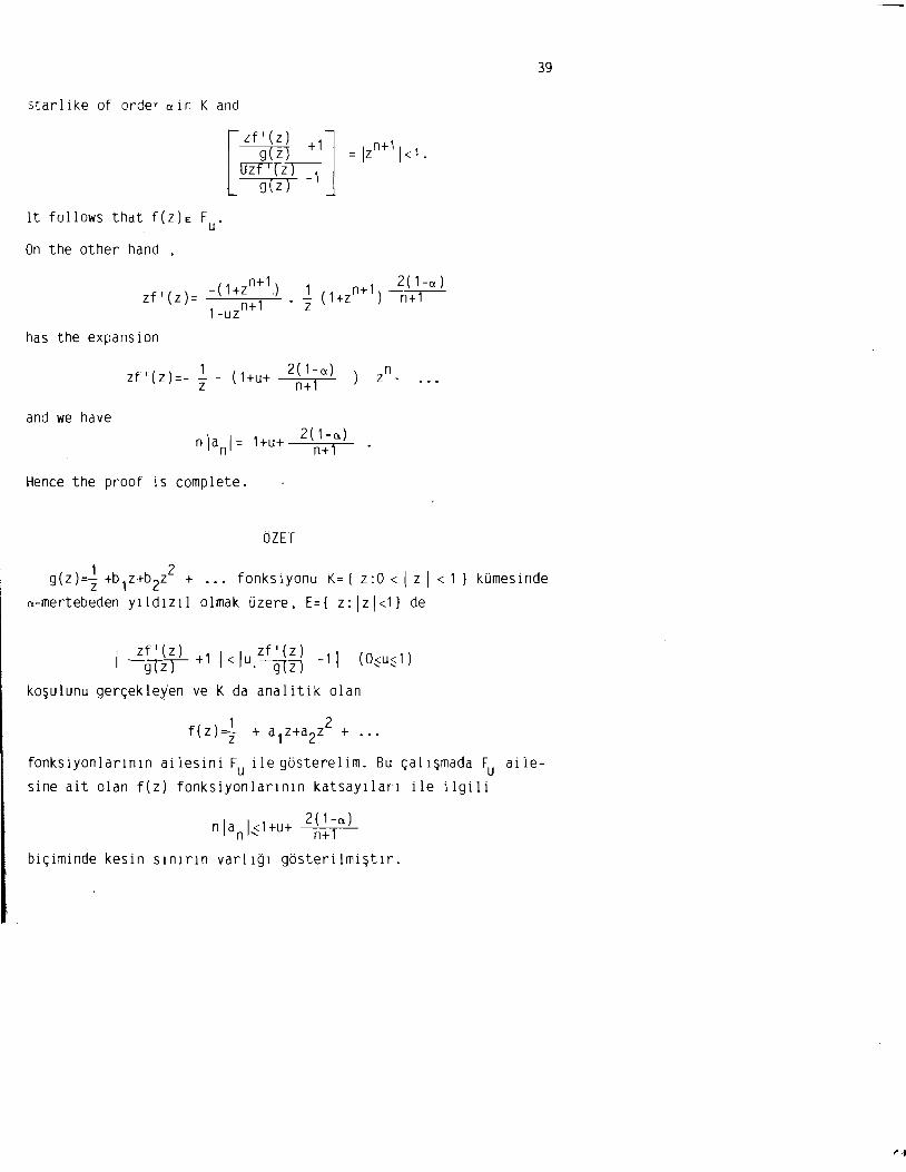
39

starlike of order ain K and

[

Zf l (Z) . 9 (z)

Uzf I (z ) g(z)

It follows that f(Z)E F u

On the other hand ,

_(1+z n+1.) 1 n+1)~~Zf I ( Z ) = ----'------.,.---'- ( 1-z n+ In+1 Z1-uz

has the expansion

n(1+u+ 2( 1- a )zf'(z)=- ~ z -n+ 1

and we have 2(1-a)

n janl= 1+u+ n+1

Hence the proof is complete.

OZET

g(Z)=~+b1Z+b2Z2 + fonksiyonu K={z:O<lzl<1} kUmesinde a-mertebeden y r ld i z i l olmak Uzere, E={ z:lzl<1} de

zf I (z ) 1 I I zf I (z ) 1I (O~u~ 1) I -9T"2T- + < u. ---g{Z) - - ­

ko~ulunu ger~ekleyen ve k da analitik olan

f(z)=z1 2 + .,.+ a1z+a2z fonksiyonlar i nm ailesini F i le qostere l i m. Bu cal i smada F aile­u u sine ait olan f(z) fonksiyonlarlnln katsayllarl ile ilgili

nl ank1+u+ 2~:1a)

bi~iminde kesin Slnlrln varllgl gosterilmi~tir.

40

'f

REFERENCES

1. Kaczmarski, J. On the coefficients of some classes of starlike functions. Bulletin De L'Academie polonaise Des Sciences Serie Des Sciences Math., Astr., et Phys. 1'7(8), 495-501, 1969~

2. Nehari, Z. Conformal mapping, New York. McGraw Hill 1952.

3. Owa, S. A remark on certain c laSses of analytic functions. Math.

Japonica 28 (1),15-20,1983.

4. Pommerenke, CH. On meromorphic functions. Pacific Journal of

Math. 13, 221-235, 1963.

41 Hacettepe Bulletin of Natural Sciences and Engineering

1985/ VolWle 14/pp. 41-52

A CHARACTERIZATION OF UNITS IN ZS4

A. VI Imaz( 1)

In this work we characterize the units in the integral group ring ZS4 by using their images in certain general linear groups under the distinct inequivalent irreducible 'repre­sentations of the group S4' The group of units in ZS4 Of a­ugmentat ion 1 is shown to be isomorphic wi th a certain subgroup. of GL(2,Z)~GL(3,Z)~GL(3,Z) .

Key words: Group, Ring, Representation, Unit, Character 1980 Subject Classification: 16A26

1. INTRODUCTI ON

Let U(ZG) denote the group of units of the integral group ring

ZG of a group G over the ring Z of integers. Hughes and Pearson

[4]and Allen and Hobby[ 1] gave characterizations of U(ZS3) and

U(ZA4), respectively. Milies[3]did the same for U(ZD4). Dennis

[6] and Sehgal [5] pointed to the need for additional work with

some small groups, inc ludi ncdetermi nat ion of the units of the ra­

tional group ring QG. In this article we restrict ourselves to in­

tegral group rings and obtain a characterization of U(Z54), where

S4 is the symmetric group,of degree 4.

Let V(ZG) denote the units raig i in ZG which have coefficient sUm

The technique used by Hughes and Pearson consists of making ra i=1. use of the distinct irreducible inequivalent representations of 53

to obtain a 6x6 matrix P that describes a faithful representation.

(1) Hacettepe University, Faculty of Science, Ankara. TURKEY.

42

Q

e :V(ZS3) -/" e(V(ZS3))CGL(2,Z).

When r=LaigiEZs3, the entries of e(r) are obtained from the matrix

product ap=B, wherea=[a la 2... a J is the row-matrix of coefficients of6

r. Finally, by computing the inverse matrix p-l and solving the linear

system of congruences obtained by requiring that a=f,p-l have entr-i es

in Z, they obtained necessary and sufficient conditions that descr-ibe

the matrices in GL(2,Z) which belong to e(V(ZS3)).

2. RESULT

Just following this method, we use the inequivalent irreducible

representations of the group S4 to find conditions determining the

elements of U(ZS4). The group S4 can be generated by the cycles a=(12)

and b=(234) which are subject to the relations 2=b 3=(1) ab2=(ba)3.a and

We agree always to list the elements of S4 in accordance with the

conjugate cla',',~s In the tol lodm

~(12)=a =gi

(13)=bab2 =g3

(14)=b2ab =g4

(23)=abab2a =g5

(24)=ab 2aba =g6

(34)=ab2abab2 =g7

(1234)=ab =q16 (1243)=ab2

=g17

(1324)=bab =CJ 18 (1432)=b2a

=g19 (1342)=ba =g20 (1423)=b2ab2

=g21

order: . 2 (123)=bab a =g8

(124)=b2aba . =g9

( 134)=aba =glO (234)=b =g11 ( 132)=abab2

=g12 (142 )=ab2ab

=g13 (143)=ab 2a

=g14

(243)=b2 =g15

( 12 )(34 )=(bab)2

( 13 )(24) =(ab )2 [ (14)(23)=(ab2)2

The group S4 has five inequivalent irreducible representations

43

P1 ,P2,P3,P4 and Ps of degrees 1,1,2,3 and 3, respect ive l y; P1 being

the 1-representation and P2 the representation assigning to each

cycle its sign. For ease of computation we choose the representations

P3,P4' and Ps slightly different from those arising naturally from

Young diagrams:

P1 (a) = 1 P1(b)

P2( a)

P3( a) =

-1

=I~A ~

P2(b)

P3(b) B G -J-1

1

.4(a) : C : ~ a -1 ~

P4(b) 0 ~ a a n

a 1

PS(a)=-c= 'a~O -1

a 1 a

-~ .s(b) : D : ~ a a ~

Let P1 Q) P2Q) P3Q) P4Q)PS denote the direct sum of the i rreduc i bIe

representations of 54' When gE54, p(g)=X* is a 1Ox 10 matrix with

blocks on the main diagonal as follows:

x1- -x2 x 0

­

x43 x .. (2.1)X* :: "s 6 x xx7 s 9

x10x 11 x12 x13 x14 x 15 D

3

n x16 x17 x18 x19 x20 x21 x22 x23 x24

, ­' ­

vk lj~e K,X"X dlld X to dpII()ll', IP',pl'ctlvely, tile d i aqona l 2 3

mdtl'l' wltll x"X;; (ill tIll' ma i n dld'J':lldi: 1111 /x'c' fild:' j, wt)(;, (' Plit·

ru: !Ii' '3'x tilt, .:1>-.1 IllJllIA Will,~'-' eut.r t es dre x7.x S •. ·.,4,x 5"u,

44

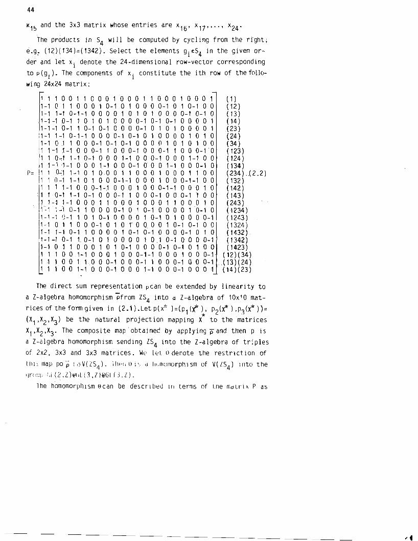
~15 and the 3x3 matrix whose entries are Xl?"'"x16' x24·

The products in S4 will be computed by cycling from the dght;

e.g: (12)(134)=(1342). Select the elements giES4 in the given or­

d~r and let Xi denote the 24-dimensional row-vector corresponding

to p (g ). The components of x . const i tute the i th row of the follo-I I

wing 24x24 matrix:

111001100010001100010001 1-1 0 1 100 0 1 0-1 0 1 000 0-1 0 1 0-1 0 0 1-1 1-1 0-1-1 0 0 0 0 1 010 1 0 0 0 0-1 0-10 1-1-10-1101010000-10-10-100001 1-1 -10 -1 1 0-1 0-1 0 0 0 0- 1 0 1 0 1 0 0 0 0 1 1-1 1""1 0-1-1 0 0 0 0-1 0-1 0 1 0 0 0 0 1 0 1 0 1-1 01 1 0 0 0-1 0-1 0-1 0 0 0 0 1 0 1 0 1 0 0 1 1-1 :1-1 0 0 0-1 1 0 0 0-1 0 0 0-1 1 0 0 0-1' 0 1 1 0-;1 1-10-10 0 0 1-1 0 0 0-10 0 0 1-1 0 0 1 1-1 '1-1 0 0 0 1-1 0 0 0-1 0 0 0 1-1 0 0 0-1 0

P= 1 , 0-,1 1-, 0 1 0 0 0 1 1 0 0 0 1 0 0 0 1 1 0 0 1 1 0-1 1-10 1 0 0 0-1-1 000 1 0 0 0-1-1 0 0 1 1 1 1-1 0 0 0-1-1 000 1 0 0 0-1-1 000 1 0 1 10 -1 1-1 0-1 0 0 0-1 1 0 0 0-1 0 0 0-11 0 0 1 1-1 1-1 000 1 1 000 1 000 1 1 000 1 0 j'~ 1. 1-'1 0-1 1 0 0 0 0":'1 0 1 0-1 0 0 0 0 1 0-1 0 1-1-1 IJ-1 1 0 1 0-1 0 0 0 0 1 0-1 0 1 0 0 0 0-1 1-1 0 1 1 0 0 0-1 0 1 0 roo 0 0 1 0-1 0-1 0 0 1-1 1-1 0-1 1 0 0 0 0 1 0-1 0-1 0 0 0 0-1 0 1 0 , -1 -1 0-1 to -1 0 1 0 0 0 0 1 0 1 0-1 0 0 0 0-1 1-1 0 1 1 0 0 0 1 0 1 0-1 0 0 0 0-1 0-1 0 1 0 0 1 1 1 0 0 1-1 0 0 0 1 0 0 0-1-1 0 0 0 1 0 0 0-1 111 0 0 1 1. 0 0 0-1 0 0 0-1 1 0 0 0-1 0 0 0-1 1 1 1 0 0 1-10 0 0-1 0 0 0 1-1 0 0 0-1 0 6 0 1

( 1) (12) ( 13) ( 14) (23) (24 ) (34 ) ( 123) (124) (134) (234) ..( 2 .2 ) ( 132) (142) (143) (243) (1234 ) ( 12Ll3 ) (1324) (1432) (1342) ( 1423)

( 12)( 34) ( 13)( 24) (14)(23)

The direct sum representation pcan be extended by linearity to

a Z-algebra homomorphi~m pfrom ZS4 into d Z-algebra of 10x10 mat­

rices of the form given in (2.1).Letplx1' )=(P1(x*~' P2(X*),Pj(X*))=

be the natural projection mapping X to the 'matrices(X1,X2,X3) The composite mapobtained by applyingpand then pisX1,X2,X3.

a Z-algebra homomorphism sending ZS4 into the Z-algebra of triples

of 2~2, 3x3 and 3x3 matrices. We 1<'1 0 denote the restrict Ion of

t hi , map pop I \)V(ZS4)' 111PII 0 i-, d II'Jmomorphism of VllS ) Into the4

qn :III! :, i (2 , Z) llillL( j , Z )&IG I (j , Z) •

lhe nomomorptu sm e cen be described III terms of t.ne ma t ri x P as

45

follows: 24

Letcx=[a 1a2.·.a24] represent the element r=i;'1 aig i, where the supporting elements gi are listed as mentioned before~ It follows

tuat the matrix product aP=x* gives the row-vector x" associated

with p(r)=X*. Then 8(r)=P(x*). The image of V(ZS4) under 8consists

of the elements (X of GL(2,Z) (j) GL(3,Z) (j) GL(3,Z) which are1,X2'X3) projections of those matrices X* such that aP=X~ where ais the row­

vector of coefficients of some rEV(ZS4)' Thus, once p- 1 is known,

we can say that the range of e is contained in the set of all (X 1'.'- -1X in GL(2,Z) (j) GL(3,Z) (j) GL(3,Z) such that X"P is a row­2'X3) vector of integers whose sum is 1.

The matrix P can be inverted using Schur relations, as mentioned

in [1,2]. We list the steps of this inversion process for the sake

of ccmpIeteness , (Pk's are the irreducible representations of S4

(1) Determine the fixed i,j and k such that the mth column of P

consists of {Pk(g)ij I gES4}· (2) Once i,j and k are known, select the column of P; say the

mtt h column, which consists of {Pk(g)ji I gES4} .

(3) Rearrange the mtt'l co-lumn by interchanging the entries for

Pk (g)ji and Pk (g-1)ji' Then multiply each entry by nk/24 where

nk is the degree of Pk .

(4) Transpose the result of step (3) to obtain the mth row of p-1 .

--------------------------------

46

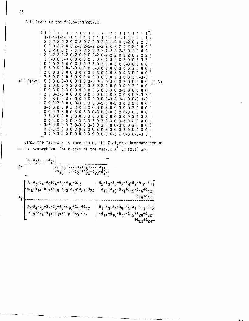
This leads to the following matrix:

111111111111111111111111 1-1-1-1-1-1-1 1 1 1 1 1 1 1 1-1-1-1-1-1-1 1 1 1 2 0 2-2-2 2 0 0-2 0-2-2 0-2 0 2-2 0 2-2 0 2 2 2 o 2 0-2-2 0 2 2-2 2-2-2 2-2 2 0-2 2 0-2 2 0 0 0 o 2-2 0 0-2 2-2 2-2 2 2-2 2-2-2 0 2-2 0 2 0 0 0 2 0-2 2 2-2 0-2 0-2 0 0-2 0-2-2 2 0-2 2 0 2 2 2 3 0-3 0 0-3 0 0 0 0 0 0 0 0 0 3 0 0 3 0 0-3 3-3 o 0 0 3-3 0 0 0-3 0 3 3 0-3 0 0 3 0 0-3 0 0 0 0 o 3 0 0 0 0-3-3 0 3 0 0-3 0 3 0 0-3 0 0 3 0 0 0 o 0 0 3-3 0 0 3 0-3 0 0-3 0 3 0-3 0 0 3 0 0 0 0 3-3 0 0 0 0-3 0 0 0 0 0 0 0 0 0 0 3 0 0 3 3-3-3 o 0 3 0 0-3 0 0 3 0 3-3 0-3 0-3 0 0 3 0 0 0 0 0 o 3 0 0 0 0-3 0-3 0 3-3 0 3 0 0 0 3 0 0-3 0 0 0 o 0 3 0 0-3 0-3 0-3 0 0 3 0 3 3 0 0-3 0 0 0 0 0 3 0 0-3-3 0 0 0 0 0 0 0 0 0 0 0-3 0 0 3 0-3-3 3 3 0 3 0 0 3 0 0 0 0 0 0 0 0 0-3 0 0-3 0 0-3 3-3 o 0 0-3 3 0 0 0-3 0 3 3 0-3 0 0-3 0 0 3 0 0 0 0 0-3 0 0 0 0 3-3 0 3 0 0-3 0 3 0 0 3 0 0-3 0 0 0 o 0 0-3 3 0 0 3 0-3 0 0-3 0 3 0 3 0 0-3 0 0 0 0 3 3 0 0 0 0 3 0 0 0 0 0 0 0 0 0 0-3 0 0-3 3-3-3 o 0-3 0 0 3 0 0 3 0 3-3 0-3 0 3 0 0-3 0 0 0 0 0 0-3 0 GOO 3 0-3 0 3-3 0 3 0 0 0-3 0 0 3 0 0 0 o 0-3 0 0 3 0-3 0-3 0 0 3 0 3-3 0 0 3 0 0 0 a 0 3 0 0 3 3 0 0 0 boo 0 0 0 0 0-3 0 0-3 0-3-3 3

(2.3)

Since the matrix P is invertible, the Z-a1gebra homomorphism ~

is an isomorphism. The blocks of the matrix X* in (2.1) are

K=

X -r

a1+a3-a4-aS+a6-aS-a10-a13

-a,S+a16-a'7+a19-a20+a22+a23+a24

a2-a4-aS+a7-a8+a9-a10+a11+a12

-a13+a14-a1S-a17+a18-a20+a21

a2-a3-a6+a7+aS-a9+a10-a11

-a12+a13-a14+a1S-a16+a1S -a 19+a21

a1-a3+a4+aS-a6-a9-a,,-a12

-a14-a16+a17-a19+a20+a22 +a23+a24

47

al-a3-a6+a16

+a19-a22+a23-a24

a4-aS+aS-al0

-a13+alS-a17+a20

a2-a 7-a 9+a11

-a12+a14+alS-a21

al+a3+a6-a16

-a19-a22+a23-a24

..., a4-aS-a9+all : (2.4)

+a12-a14+a17~a20 , -a13+alS-alS+a21

a2-a 7-a S+alO

-----------------t----------------­a1-a2-a7+a1S a3-a6+a9+al1

+a21+a22-a23-a24 -a12-a14-a16+a19-----------------1-----------------­

! al-a4-aS+a17a3-a 6-aS-a lO

+a13+alS+a16-a19 II +a20-a22-a23+a24

-a4+aS-a9+all I -a2+a7-aS+al0 I

+a12-a14-a17+a20! -a13+alS+alS-a21

=~~:~~:~~=~~~--- -~~:~;:~;=~~~----l-=~;:~~:~~:~~~-----

~:~:::~=::~::::~--:::~:::::::::::~~-::~:::~~::~~::~:---a3+a6-aS-al0-a 2+arag+a11 I a1+a4+aS-a 17

-a12+a14-alS+a21 +a13+a1S-a16+a19 -a20-a22-a23+a24

Consider a vector x*=( x •.. 'x The vector (a l,a2.. ,a 2LlJ1,x2' 24]. whose image under e is x* wi 11 be computed from the product x* p-l.

For each of a i to be an integer, the system x*p - \:O( mod 24) must beso 1ved.

We list some properties of the matrices Xl 'X and X which can be2 3 drawn from the forms of these matrices (2.4'.

l3 x~ ,. 7 Xs xg UFor X X = x x xl= Xs x 2 10 l l 12;6 x x x13 14 l S f

we have

(a) in Xl: x (mod 3)3+xS=x4+x6 (b) in x7+xl0+x13::xS+x1l+x14 ::X9+x12+x1S (mod 2)X2:

in x16+x19+x22=x17+x20+x23::xlS+x21+x24(mod 2) X3: (c) the corresponding entries of X and X are congruent (mod 2):

2 3 xl,:x IC (mod 2); x (mod 2) ; ... ; x (mod 2)

H=-x 17 1S=-x 24

1(1 .lescribe "0111i:' lither' re l a t lUll' l'I" ''''''''1. lilt' rn i l r It t,S X !lId X;,3

we dd,f1~-Ltle t o i Iowi uq surns dliLl pro.luc t s :

48

4

I, = x7xl1x15

12 xSx12x13

,I3 x9x'Ox'4 14 =-x 9x"x'3 t 5 =-x8x'Ox'5 t 6 =-x 7x'2x'4

t, = x16 +x20 +x24 'q x16x20x24 t 2=-x 17 +x21 -x 22 t 2 x17x21x22

t 3 =-x'8 +x19 -x 23 t 3 x18x19x23 t 4= X18 -x 20 +x22 'f4 =-x 18x20x22

t s= x17 +x19 -x 24 t s =-x 17x19x24 t 6=-x 16 +x21 +x23 f 6 =-x16x2,x23.

In terms of these t and t k s we have the following relationsk between X2 and x3: (k=1, .•.• 6)

(d) Let xi and be any two elements of X belonging to t k andxj 2 let xi and xi be the corresponding elements of X3 in t k . Then

(a ') IfXi,xj(respxi,xj)belongtot1,t2 ort3(resp.ti,t2ort3)then x.+x .=-(x!+x') (mod 4) and x, -x .=-(x' -x!) (mod 4)

1 J 1 J 1 J 1· J

(b ') If Xi ,x (resp. xi ,xj) belong t 6 (resp.t4,tsj to t 4,t5 or

or t 6) then

X.+X. =x'.+x! (mod 4) and x.vx . =x~-x~ (mod 4).IJ IJ . IJ IJ

We know that for a vector x" to belong to e (V(ZS4)) a necessary

and sufficient condition is that the vector x* satisfy the congru­

ences x* p-' =0 (mod 24). This gives 24 equations represented by

the matrix equ ali ty [a, ,a2, ... ,a ] = x* p-1 for calculating the24 integers a"a2, ... ,a24•

24Summing up these equat ions we see that L i=l a = 24x,l24=xi l,

from which we derive the conclusion that the first component Xl of

the vector x* must be chosen to be 1. Because the diagonal entries

49

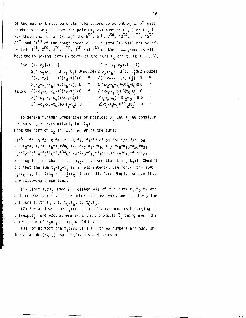
of the matrix K m~st be units, the second component xz of ? will be chosen to be j 1. Hence the pair (x1;xZ) must be (1,1) or (1,-1).

7t h, 10t h, 11 t h, 1Zt h, For these choices of the 5t h, 6th,(x1,xZ)Z3 rd and 24t h of the congruences x* p-1 ~O(mod 24) will not be at ­

1st, 2nd, 3rd, 4t h, 8t h andfected; 9t h of these congruences will have the followi ng forms in terms of the sums t k and t k.(k=1 , ... ,6).

For (x, ,x2)=(1,1) For (x1,x2)=(1,-1)

2( 1+x3+x6) +3(t 1+t; )=0(mod24) 2(x3+x6) +3(t 1+q )=0(mod24) 2(x4+x5) +3(t4-t,p=0 2(1+x+X5)+(t4-t4) =0II II

2(x3-x5-x6) +3(t6-ttP=0 II 2(1+x3-><s-~)+3(t6-tf)=:° " (2.5). 2( -x3-x4+x6)+3(t5-t~P=0 " 2(1-x3-x4+~)+3(t".s-tS)= 0 II

2(1+x4-x5-x6)+3(t3+t3)=0 2(»f><s-~)+3(t3+t3) =0II

2(1-x3-x4+x5)+3(~+"t2)=0 " 2(-~-x4+><s)+3(t2+t2) =: 0 II

To derive further properties of matrices X2 and X3 we consider

the sums t i of X2(similarly for X3). From the form of X2 in (2.4) we write the sums:

t1=3a1-a2-a3-a4-a5-a6-a7+a16+a17+a18+a19+a20+a21-a22-a23-a24

t2=-a2+a3-a4+a5-a6+a7+3ag-d11-a1Z-a14-a16-a17-a1S+a19+a20+a21 t3=-a2-a3+a4-a5+a6+a7+3aS-a10-a13-a1S-a16-a17+a1S+a19+a 20-a 21.

Keeping in mind that we see that t 1+t2+t3+1 =O(rocd 2)a1+ ...+a24=1, and that the sum an odd integer. Similarly, the sumst 1+t2+t3 is

t;+t2+t3 and odd. Accordingly, we can listt 4+t5+t6, t 4+tS+t6 are

the following properties:

(1) Since ti=ti (mod 2), either all of the sums aret 1,t2,t3 odd, or one is odd and the other two are even, and simi Iar ly for

the sums t"t2,t3 ; t 4,ts,t6; t 4,tS,t6. (2) For at least one t.(resp.t~) all three numbers belonging to

1 1 ti(resp.ti) are odd; otherwise, all six products t i being even, the determinant of X2=t1+ ...+t6 would beF~l.

(3) For at most one ti(resp.ti) all three numbers are odd. Ot­herwise be even. det(X2),(resp. det(X3)) would

50

Accordingly, for the matrices X2 and x~, for exactly one t i ai 1 three numbers belonging to these t. ,t! are odd, the remaining

1 1

elements of these matrices are even. (4) If the odd entries of X2 and X3 belong to t l and ti then

at least one of the entries on t2,t3(t2,t3) must be divisible by 4.

(mod 3)} C GL (2 ,Z)

xa xg ~ co1umn sums are congruent (mod 2)} "u and exactly one t i contains odd CGL(Z,3)x12

entries; the other entries allx14 x15 being even.

G3cGL(3,Z) defined similarly for GZ. Now let G=G Q G2 Q G31

" Q GL(3,Z) IXl 'X2' X{ (X l,X2, X3)EGL(2,Z) Q GL(3,Z) 3 satisfy conditions (a)-(d) and (2.5) J.

Then G is a group containing e(V(ZS4)) and we can characterize the group of units under consideration as fQllows:

2.1. PROPOSITION.

Proof. The only thing we need to show is that e :V(ZS4) ->G is an isomorphism and that the inclusion e(V(ZS4))cG is an equ ­ality. Let 12 and 1 denote identity matrices of order 2 and 3,3

resp. and K the diagonal matrix with entries xl,x2• Consider the matrix

K I

]*X "

r If wf·III)(J, "l,'.:i i her thdfl II.li: t nat iS,if ()(j,x

2 )=(l , -1) ,

tiler, Wl tjt'l :1'UrTl t he f,rrJduct -""'1,-1. "l,lrles other' than integers;

e.g. the first four entries of x*p- l are 11/12, 1112, 1112 and 1112

I

51

Therefore, the natural projection p restricted to P(V(ZS4)) has trivial kernel. Since p is already an isomorphism, it follows that 6 ~ an isomorphism.

Finally, we show thateis onto by observing that [a" ... ,a24]: x*p-' has integer entries. Choose From the forms of(X"X2,X3)EG. the blocks in (2.4) we obtain, by a long computation, the congru­ence

det(X, ):x 3x6-x4x5 =x,x2 (mod 3):: x2 (mod 3)

from which we determine the second entry of K to be x2=det(X,).Now we use the choice (x"x2)=("det(X,)) toqether with the entries of X1,X2,X3 to determine the vector x*= [x 1, ... ,x24]=[', detX"x3

the vector of coefficients a= [a 1, ... ,a 24]for, ... ,x24]and find an element r=Iai9i in V(ZS4) which satisfies the equality aP=x*. That the coefficients a1,a2,a3,a4,a8 and a9 are integers follows from the conditions (2.5) and that the remaining coefficients are integers from conditions (a), (b), (c), (d).

Example. We observe that the triple

~ 5 2 -30 -21]

-6 -3 -2 ) -57 -34 -24

belongs to the group G described above. Because det (X 1)=-1 we ma­

ke the choice (x"x2)= (1,-') and form the vector x*= [1,-' ,46,-19,-63,26,4,-30,33,-6,51 ,-58,-3,22,-24,-52,-30,-21,

-6,-3,-2,-57,-34,-24]. Now the product x~'~1 gives the vector

a= [0,0,0,0,O,u,-27,0,0,6,-30,0,0,0,0,28,0,0,0,0;24,0,0 ]

'with non-zero entries a7=-27,a1Q=6,a11=-30,a16=28, a22=24 group ring elementand a,+ ...+a24=1.Hence the

r=a7g7+a10g10+a11g11+a16916+a22g22 :-27(34)+6(134)-30(234)+28(1234)+24(12)(34)EZS4 '. -1 -1 ( -1-1IS a unIt with inverse r EZS4 determined by a = x*) P ; where (x*)-1 is a vector obtained by using 1, detX 1 and the entries of

52

1 -1 -1the matrices X, , X ' X . Si nce 2 3

-1 -1 -1 [- 26 - 19l ~5 ~ ~ 7J ~4 6 ~l (X 1 'X2 'X3 ) =( -63 -461, ~1 2 24 , t~~-§~-~~ )

and det(x,1 )=-1 ,we again make the choice (X ,X ,-1) and form1 2)=(1

(x)* -1 =[ 1, -1,-26, -19, -63, -46,52,6,57,30,3,34,21,2,24,-4,6,3,30

-51,-22,-33,58,24].

Accordingly, -1 (*)-1 -1 a = X P =[0,0,0,0,0,0,-27,0,0,0,0,0,0,-6,30,0,0,0,

28,0,0,-24,0,0]

with non-zero elements a7=-27;a14=-6;a15=30;a19=28;a22=-24, 1and the desired inverse element r- is obtained as

-1 r =a7g7+a14g14+a15g15+a19g19+a22g22

=-27(34)-6(143)+30(243)+28(1432)-24(12)(34).

bZET

Bu cal i smade Z54 grup na lkas iru n bi rimselleri, 54 grubunun f ark l i

denk olmayan indirgenemez representasyonlan a l t mdak i muayyen genel

lineer gruplar i c t ndek i gorUnUmleri kul l aru l arak karakterize edi lmi s

olup, Z5 de ogmentasyonu 1 olan birimseller grubunun GL(2,Z) ~ 4 GL(3,Z) i GL(3,Z) nin bir alt grubuna izomorf o Iduqu gosterilmi~tir.

REFERENCES

1. Allan, P.J and Hobby, C. A characterization of units in ZA4,J. Algebra 66,534-543, 1980.

2. Hall, M. The theory of groups, Chelsea, New York, 1976.

3. M~l~es, C.P. The units of the integral group ring ZD4,Bol.Soc.Math.Brasil 4,85-92,1972.

4. Hughes 1. and Pearson, K.R. "The group of units of the integral group ring ZS3' Canad.Math.Bull.15, 529-534 1972.

5. Sehgal, S.K. Topics in group rings Dekker, New York, 1978. 6. Denn~s, R.K. The structure of the unit group of group rings

Lecture notes in pure and applied math. vol.26; Dekker, New York 1977.

53 Hacettepe Bulletin of latDral Sciences and Engineering

1986/ Volu~ 15/pp. 53-59

A NOTE ON FUZZY NEARLY COMPACT SPACES

This paper discusses fuzzy near compactness in fuzzy to­pological spaces. We give some characterizations of fuzzy near compactness in terms of regular open and regular closed fuzzy sets.

Key Words: Fuzzy topological spaces, Fuzzy near compactness

1980 Subject Classification: 54A40

1. INTRODUCTION

Zadeh in [8] introduced the fundamental concept of a fuzzy set. Fuzzy topological spaces were first introduced in the literature by Chang [2] , who studied several basic concepts including fuzzy continuous maps and compactness. In this paper we study fuzzy nearly compact spaces. We give some characterizations of near compactnes in terms of reguIar open or reguIar closed fuzzy sets. We first give some necessary preliminaries.

Let Xbe a nonempty set and F(X)= {fIf: X--;>[ O,1]} • The elements of F(X) are called fuzzy subsets of X[8] . We denote by Ox and 1 the functions on X identically equal to °and 1 respectively. x

Now we recall that a fuzzy topology in the sense of Chang [2] is a subset t of IX such that x

(t ) 0xEtx and 1xEtx'

(1) Hacettepe Univ.Fac.of Science, Mathematics Dept., Ankara,TURKEY

54

A collection {fi} id ,where fiE\, iEl, is a cover of X iff i~Ifi=1x. A fuzzy topological space is compact iff every open co­ver has a finite subcover [2] .

Let Xbe a fuzzy topological space. For a fuzzy set of X, the clo­o

sure T and the interior f of f are defined respectively as

T=inf {g:g>f,g'E't }x and

of=sup { g:g <f, gE't } •

X

A fuzzy set f ois_ called regularly open iff f=(r)° and regularly closed iff f=(f) [1].

A fuzzy topological space X is almost compact iff every open cover has a finite subcollection whose closures cover X[ 3 ] . A

fuzzy topological space X is called nearly compact iff every open cover of X has a finite subcollection such that the interiors of ue closures of fuzzy sets in thi s collection covers X[ 4 ] .

If't x is a fuzzy topology on X, a collection B£-rxis a base of 't iffeachf£'t is of the form .VIf., where f.EB,Vi; and its mem­x x 1£ 1 .1 bers are called the "basic open sets of the topology r ". A col­x lection ~'t is a subbase iff {f.A •.. Af · } fiES is a base ot e.. x 1 1 1n x

2. RESULTS

The following theorem shows that we may work with fuzzy regularly closed or fuzzy regularly open sets:

2.1. THEOREM. In a fuzzy topological soace X with base B the fol­lowing conditions are equivalent:

(i) X is nearly compact.

55

(ii) Every basic fuzzy open cover of X has a finite subcollec­

tion such that the interiors of cLosures of fuzzy sets in this

subcollection covers X.

(iii) Every cover of X by fuzzy regularly open sets has a f ini te

subcover.

(IV) Every collection of fuzzy regularly closed sets having the

finite intersection property has nonempty intersection.

(V) Every collection {f i} id of fuzzy closed sets having the

property that for any finite subcollection {f.: i=1, ... .n) of n 0 1

{f i} id' i~1(fif#Ox' has nonempty intersection.

Proof. (i=:>ii) follows easily.

(ii==>iii). Let {f i£I be any fuzzy regularly open co­i} ver of X and let B be a base for ~x. For each i£I,

f i= V {9j:jd i, 9{B} Then A= {gj: jd iEl} is a basic openi,

cover of X. By(ii), A has a finite subcollection {gk:k=1, •.. ,n } n -

such that k¥1 (9k P=1 x• Now for each k=1,2, ... ,n there exists a

f k£ A such that gks. f Therefore we have (9k)°S.(f'k)0=fk andk• n

k~1 f k=1x:

(iii ==>iv). Let {gil id be a collection of fuzzy regularly

closed sets with the finite intersection property and suppose that

.A g.=o . Then {1-g.} . I is a collection of fuzzy regularly1£I 1 XIIe

open sets with the finite interspction property and by assumption

there existsa finite subset F~I such that iYF This(1-g i)=1 X. implies .AF9·=ox' W"iich is a contradiction. Hence l·AI g.#o .1£ 1 e 1 x

(tv ==>v) . Let {g.}. I be a collection of fuzzy closed sets1 1£

having the given property. Then {(8·)-} . I is a family of fuzzy1 1£ regularly closed fuzzy sets having the finite intersection property.

o 0 By (tv ), i~I (gi)-#Ox' But, from (gi)- S.gi we have i~l gi#Ox'

56

(v =>i). Let {f.} I be a fuzzy open cover of X.0

1 lE

If loVF (fo)o does not cover X for every finite subcollection e 1 \

{fi } iE:F' then i~F (v), i.e.((l-f i)o)-#ox· By ih (1-f i)#oX'

i~l (1-(1-f i))#l x and hence the contradiction i~I f i#l X· Obviously every nearly compact fuzzy topology is almost compact.

The reverse imJi ication does not hold in general:

2.2. EXAMPLE. Now let X={a,b,c,d} and .x be the fuzzy topology with subbase

where 1 1 1

f n(a)=l- n ' f n(b)=l- n ' fn(c)= L ' 1

f n(d)=l- n 1 1kn(a)= n ' kn(b)= ~' kn(c)=O, kn(d)=O,

Then (X"x) is almost compact but not nearly compact.

2.3. REMARK. This example may also be used to show that one cannot replace "base" by "subbase" in Theorem 2.1. (ii). For consider the subbase {Pn'qn,r } wheren,hn,kn:n=1,2, •.•.

P = (V (fnAgn)) V fn'n n

Q = (V (fnAg n)) Vgn n,n

r =f Vg •n n n

For this family B the condition (ii) of Theorem 2.1 is satisfied - 0 - 0 - 0

since (Pn) =(qn) = (rn) ='x· However as we have noted this fuzzy

57

topological space is not nearly fuzzy compact.

Recall t.he t a fuzzy space (X.'tx) is called a fuzzy semiregular space iff the collection of all fuzzy regularly open sets of Xforms a base for the fuzzy topology 't [ 1 ] .x 2.4. THEOREM. A nearly compact semiregular fuzzy topological space X is compact.

Proof. Let {fi}iEI be an open. cover of~. that is i~I f i=1 x' Since X is semi requl ar , f,=,V I g.~ • where gJ~ is a fuzzy regularly

1 J E i J

open set. But. from ,V I 'V I g~ =1 X' there exists a finite subcol-IE JE i J n

lection {gk: k=1, ... ,n} such that k~1 gk=1 x' Now for each k=1, • ... ,n t~ere exist' a f k in {f i} id such that gkS.fk' Hence we have k~1 as required.f k=1 x 2.5. COROLLARY. A fuzzy semiregular space is nearly compact iff it is compact.

Proof. This is immediate from Theorem 2.4.

In Azad [1] some weaker forms of continuity, fuzzy semicontinuity fuzzy almost continuity and fuzzy weak continuity, are considered for the first time. For a fuzzy almost continuous function we have: A fUzzy almost continuous image of an almost compact fuzzy topolo­gical space is almost compact [3] and a fuzzy strongly continuous image of an almost compact space is compact [4] . The same holds for nearly compact spaces:. . 2.6.COROLLARY. An almost ccrntinuous image of a fuzzy nearly compact space is fuzzy almost compact.

2.7. COROLLARY. The image of a fuzzy nearly compact space under a strongly continuous mapping is compact.

The proofs are simi larto the almost compact case, and areanitted.

A. Di Concilio and G. Gerla [3] studied products of fuzzy almost compact topological spaces and proved that in general almost com­pactness for fuzzy topological space is not product invariant.

58

although if X and Yare almost compact fuzzy topological spaces

and if X is product-related to Y, then their fuzzy topological

product is almost compact. Recall that a fuzzy space X is product related to another fuzzy space Y, if for' any fuzzy set f of X and

g of Y whenever h'lf and k'ig implies (h'x 1)V(1 x k') ~fxg, whe­

re h£'t and ke r y' there ex i sts h1£'tl: and k1e r Y such that h\~f orx k:~ and (h~XI)V(IXk~)=(hlxl)V(lXk) [1] Itilere hi and k' are the

complements of hand k, respectively. If f is a fuzzy set of X, g

a fuzzy set of Y and Xis ptoduct-re1ated to Y, then f x g=fxg holds[1 J. We omit the proof which is simi lar to the almost conact case.

2.8. COROLLARY. If (x,'tx),(Y, 'ty) are nearly c~pact fuzzy topo­logical spaces and X is product-related to Y, then their fuzzy to­

pological product is nearly compact.

A product of two nearly compact fuzzy topological spaces need

not be nearly compact.

2.9. EXAMPLE. Let X be a nonempty set,

't ={ faE f (X) : a>~} U{ox}

and

where we denote by f the fllrtioo 00 X identically equal to a[ 3] • OU .

We have that (fa) ='X' )L faE't, a#O. Then 't is nearly compact since every open cover of 't* must contain 1 and then also 't* is x nearly compact. Their standard product is (f1EF(XxX): 0;S1<1}.

Then (fl)o=f 1 , )L 1. Thus the open cover {f1}, 0 $.1< 1, does not

contain any finite proximate subcover.

Acknowledgment. The author would like to thank Asoc, Prof.Dr. Do­gan ~oker and Dr. Lawrance Brown for some very helpful suggestions.

59

oztr

Bu ~all~mada belirtisiz topolojik uzaylarda yakln tlklZllk in­celendi. Belirtisiz yakin t ik i zl i qm belirtisiz regUler acik ve regUler kapall kUmelerle karakterizasyonu verildi.

REFERENCES

1. Azad, K.K. On fuzzy semicontinuity, fuzzy almost continuity and fuzzy weakly continuity. Journal of Math. Anal. Appl. 82, 14-32, 1981.

2. Chang, C.L. Fuzzy topological spaces. Journal of Math. Anal. Appl. 24, 182-190, 1968.

3. Concilio, A. D1. and Gerla, G. Almost compactness in fuzzy topological spaces. Fuzzy sets and Systems, 13, 187-192, 1984.

4. Eli', A. Haydar. Almost compactness and near compactness in fuzzy topological spaces. Fuzzy sets and Systems, to appear.

5. Coker, Dogan and Eli', A.Haydar. On fUzzy S-closed spaces (sub­mitted) •

6. Singal, M.K. and Mathur, A. On nearly compact spaces. Boll. Un. Mat. Ital. 11,702-710, 1969.

7. ~zer, O. On lightly compact spaces. Acta Sci. Math. 116,115­119, 1983.

8. Zadeh, L.A. Fuzzy sets. Inform. Control. 8, 338-353, 1965.

Hacettepe Bulletin of Natural Sciences and Engineering 61

1986/ Vol~e 15/pp~ 61-61

MATRIX BAER* - RINGS

A. Harmanc 1 ( 1 )

Let R be a ring with involution * and R denote the ring of all nxn matrices over R. We assume every

nprime homomorphic

image of R has proper induced involution. Under this assumption it is proved that R is Baer*-ring for all n with transpose involution if and o~ly if P=P* for all prime ideals P, the induced involution on RIP is positive definite and R is a semi-hereditary ring.

KeyWords: Baer*-rings, Semi-hereditary rings, Ring of quotients

1980 Subject Classification: 16A~8

1. INTRODUCT ION

Throughout R will denote an associative ring with identity 1.

We follow the terminology of [1) in general. If R is a ring with

an involution *, we may define an involution on the nxn matrix

ring R by applying both the transpose, and the involution to n, each of its entries.

1.1. DEFINITION. Let R be a ring with involution *.The involution

is positive definite if, for all finite subsets {ri}af R,Lrir7 =0

implies all the r i are zero. An element r of R is said to be bounded if

there ex i sts a posit i ve integer k such that r~< r-ck 1. The set of all

bounded elements is denoted by R it is called the bounded subringb; of R.

(1) Hacettepe University, Department of Mathematics, Ankara. TURKEY

" jI

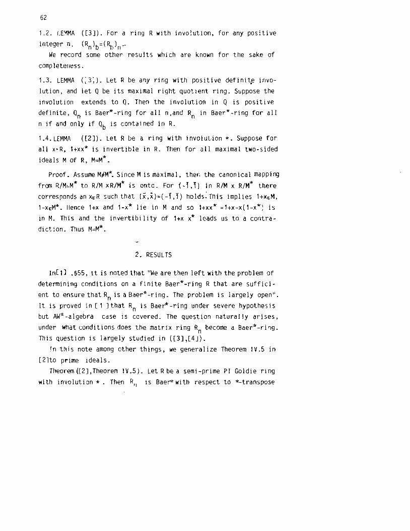
62

1.2. LEMMA ([3]). For a ring R with involution, for any positive

integer n , (Rn)b==(Rb)n" We record some other results which are known for the sake of

completeness.

1.3. LEMMA (;3~). Let R be any rir,g with positive def im te invo­

lution, and let Q be its maximal right quotient ring. Suppose the

involution extends to Q. Then the involution in Q is positive

definite, Qn is Baer*-ring for all n,and Rn in Baer*-ring for all

n if and only if Qb is contained in R.

1.4. LEMMA ([2]). Let R be a ring with involution *. Suppose for

all x-R, l+xx* is invertible in R. Then for all maximal two-sided

ideals Mof R, M=M*.

Proof. Assume M;lM*. Since Mis maximal, then the canonical mapp irq

from R/MliM* to RIM xR/M* is onto. For {-1, 1) in RIM x R/M* there

corresponds an xER such that (x,x)=( -1,1) holds: This impl ies l+xEM, l-x EM*. Hence l+x and l-x* lie in M and so l+xx* =l+x-x(l-x*) is

in M. This and the invertibility of l+x x* leads us to a contra­

diction. Thus M=M*.

2. RESULTS

In] 1] ,§55, 'it is noted that "We are then left with the problem of

determining conditions on a finite Baer*-ring R that are suffici­

ent to ensure that Rn is a Baer*-ring. The problem is largely open".

It is proved in[l ]that R is Baer*-ring under severe hypothesisn but AW*-algebra case is covered. The question naturally arises,

under what conditions does the matrix ring R become a Baer*-ring.n This question is largely studied in ([3],[4]).

Tn this note among other things, we generalize Theorem IV.5 in

[21to prime ideals.

Theorem ([2],Theorem IV.5). Let Rbe a semi-prime PI Goldie ring

with involution *. Then Rn is Baer* with respect to *-transpose

63

· .

for all n, if and only if

(a) P=P* for all primitive Ideals of R

(b) The induced involution on RIP is positive definite for all

primitive ideals P

(c) R is semihereditary.

We begin with the following

2.1. LEMMA. Let R be a ring with involution*. Suppose R has a two

sided prime ideal P satisfying

x X*E P implies XEP (xER).

Then P=P*.

Proof. Assume we have an xEP* and xiP. Then for all rER,

(rx)(x* r*)=(rx)(rx)*EP* and (rx)(rx)*EP. Since P is prime we ob­

tain rXEP from hypothesis, thus RxP and so xEP. This contradiction

proves that P=P* .

We consider the following condition in rings with involution.

(el) .. The invertibility of ltxx* implies P=P*

2.2. LEMMA. Let R be a ring with a positive definite involution.

Then for every xER ltxx* is not a zerO divisor.

Proof. Assume (ltxx* )t=O for some tER. We right multiply by ~

and we obtain ttt(tx)(t*xJ*=O. This and the positive definiteness

of involution implies t*t=O, t*x=O which implies t=O.

2.3. PROPOSITION. Let R be a semi-prime Goldie ring with involution

and assume every prime homomorphic image of R is regular ring. If

R satisfies the following conditions

1) For each primp ideal P in R,P=P*,

2) The induced involution on RIP is posi ti ve definite.

3) R l S semI-hereditary.

Then l~ is 8aer"'-rinn for all 1)()';1 11/ f - i nt.eqer II. n

Proof. R IS semi-pnme Goldie, therefore Rn is semi-prime

64 «

Goldie. The maximal ring Q(Rn) of quotients of R is semi-simplen artinian [5,(2.3.7)J , so for any subset S of Q(R the rightn), annihilator r(S) is induced from the annihilator of an element a

in Q(R Since R is semihereditary, by [3 J R is principallyn). n projective, therefore r(S)=r(a)=eR for some idempotent e€R To n n. prove R a Baer* -ring it is enough to show l+xx* is invertible n [6, Theo.26J. For if K is a primitive ideal in R then K=P for n n some primitive ideal P in R [7, page 71 J ~ Sioce each primitive

ideal is prime ideal, 1) and 2) imply P=P* and the induced invo­

lution on RIP is positive definite. Since (R/P)n=R/P and alln hypothesis of R are satisfied by R then Rn/P has positive de­n, n finite involution. Lemma 2.2 implies, in (R/P)n=R/P l+xx* isn, not zero divisor. Since RIP is regular, Rn/P is regular and therefore n l+xx* is invertible in R/P Then for each xER and for everyn- n, primitive ideal Pn, 1+xx* is invertible in Rn/Pn• Thus l+xx* is

invertible in R which proves the proposition.n

2.4. PROPOSITION. Let Rbe a semi prime Goldie ring with involution

*and assume every prime homomorphic image of R is von Neuman regular

and R is Baer*-ring with respect to transpose involution for all n n. If (el) holds for prime ideals ~ in R then

1) P=P'" for all prime ideals P,

2) The induced involution on RIP is positive definite, for all

prime ideals P in R,

3) R is semi-hereditary.

Proof. Since R is semi-prime Goldie, it has a semi-simple arti ­

nian maximal ring Q(R)=Q of quotients. Then * extends to Q and Qn is Baer*-ring and Qb the ring of bounded elements of Q is contain­

ed in RDJ.As in [2] we give a detailed proof that l+xx*is inver­

tibleinlLSlnceR2 is Baer*-ring, wetakeXER and we put X=(~ ~),

and r(X)=pR2 for some projection p in R Denote Y=(-~ ~ )ER22. and then XY=O, so YEr(X) and pY=Y and Xp=O. Since R2 has transpose

involution then p must have the from (~* ~) where a=a*. We use

55

Xp=O and pY=Y and we obtain a+xb*=O, -ax+b=-x. We apply the invo­

lution to the second and use the first equality to obtain a=xx*(1-a).

We add 1-a to both sides this equality and we conclude that 1+xx*

is invertible. We here invoke (CI) to get P=P* for every prime

ideal P of R,and so 1) follows. Let P be a prime ideal of R, then

RiP has an induced involution, and since it is regular, then RIP

is a *-regular ring [5.Theo.25J and so xx*EP implies XEP. Since

Rn/P satisfies all the hypotheses of R then XX*EP implies~Pn n n for all prime ideals P in Now we prove the induced involution n Rn• of RIP is positive definite. For this it suffices to show 1:X iXiEP implies xiEP where {xiJt;R,(i=1,2, ••• .t ) .

Set

x1 x2 Xt X= 0 0 0

0 0 0

then x*=

* x1 0 0 * x2 0 0

and

x* 0 0t

[XiX! ° *XX*= since0 0 E Pn 1:X iXiEP.

0 0 ~J HenceXEP which impliesxiEP (i=1,i, ... .t ) , It completes the proofn of 2). As for 3), R is Baer* -ring hence the right annihi lator of n any subset of R is generated by a projection (idempotent), and n therefore R is .pr inc iaa l ly projective, thus [ 3 J implies that R is n semihereditary.

2.5. THEOREM. Let R be a semi-prime PI Goldie ring satisfying (C1)

for all prime ideals with involution. Then R is Baer* -ring with n respect to the transpose involution for all n, if and only if

1) For all prime ideals P, we have P=P*,

2) The induced involution on RIP is positive definite for all

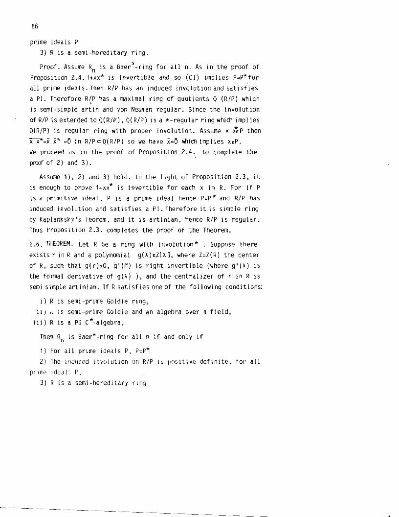
66

prime ideals P

3) R is a semi-hereditary ring.

Proof. Assume R is a Baer*-ring for all n. As in the proof of n Proposition 2.4.1+xx* is invertible and so (CI) implies P:::P*for

all prime ideals. Then RIP has an induced involution and satisfies

a Pl. Therefore RIP has a maximal ring of quotients Q (RIP) which \

is semi-simple artin and von Neuman regular. Since the involution

of RIP is exterded to Q(R/P), Q(R/P) is a *-regular ring whicr. impl ies

Q(R/P) is regular ring with proper involution. Assume x ~p then

XX*:::x x* :::0 in R/Pc:Q(R/P) so we have x:::O Wlich implies XEP.

We proceed as in the proof of Proposition 2.4. to complete the

pnxrr of 2) and 3).

Assume 1), 2) and 3) hold. In the light of Proposition 2.3, it

is enough to prove 1+xx* is invertible for each x in R. For if P

is a primitive ideal, P is a prime ideal hence P:::P* and RIP has

induced involution and sat.t sf i es a Pl. Therefore it is simple ring

by Kaplanks~v's Teorem, and it is artinian, hence RIP is regular.

Thus Proposition 2.3. completes the proof of the Theorem.

2.6. THEOREM. Let R be a ring with involution* . Suppose there

exists r in R and a polynomial g(;\)EZ[;\], where Z:::Z(R) the center

of R, such that g(r):::O, g'(lr) is right invertible (where g'(;\) is

the formal derivative of g(;\) ), and the centralizer of r in R is

semi simple artinian. If R satisfies one of the following conditions:

i ) R is semi-prime Goldie ring,

i 1 } 1\ is semi-prime Goldie and an algebra over a field,

iii) R is a PI C*-a Igebra,

Then R is Baer*-ring for all n if and only if n

1) For all prime ideals P, p:::p*

2) The induced invo lut ion on RIP 1" pos i t i ve definite, for all

prime i dea l: P,

3) R is a semi-hereditary rlng

6/

Proof. Each prime homomorphic image of R is simple artinian in the case ii). In the case i) each prime image is simple artinian.

In these cases the Theorem is clear. Case iii). R is semi-prime algebra and the hypothesis implies that each prime homomorphic i ­mage of R is simple artinian[B]. Hence each prime ideal P and primitive ideal P is maximal, therefore RIP is a regular ring.Hence the proofs of previous Propositions 2.3 and 2.4 carryover verbatim and we complete the proof.

OZET

Bu ~all~mada involOsyonlu halkalarln matris halkalarlnln Baer*

halka olmasl i~in gerek ve yeter ko~ullar ara~tlrlldl. R halkaSI­nln matris halkalarlnln Baer*-halka olmasl i~in R semi-prime Gol­die, her asal ideali P i c i n P=P*, RIP pozitif definite involUs­yonlu ve R nin semi-hereditary sert l er i rn saql amas iru n gerek ve yeter olacagl, R nin PI halka; R nin C~cebir olmasl durumlarlnda i spat l and i ,

REFERENCES

1. Berberian, S.K. Baer*-rings, Springer-Verlag, 1972

2. Handelman, D. Rings with involution, as partially ordered abelian groups, preprint.

3. Handelman, D. Coordinatization applied to finite Baer*-rings, Trans. Amer. t1lith. Sere. 235,1-34,1978.

4. Handelman, D. PrUfer domains and Baer*-rings. Arch. der. Math. 29,242-257, 1977.

5. Jategaonkar, A.V. Localization in Noetherian Rings, Cambridge Univ. Press,1986.

6. Kaplansky, I. Rings of Operators, Benjamin, 1968.

7. Lambek, J. Lectures on rings and modules, Blaisdell, 1966.

8. Rowen, L. Monomial conditions on prime rings, Isr. Jour.Mat. 23,19-30,1976.

69 Hacettepe 1IIIetin of lat.ral Scielces and [~ineeri.g

1986/ Vol... 15/pp. 69-15

SOME REMARKS ON THE COMMUTATIVITY OF RINGS

A. Harmancl(l)

Let R be a ring with identity. For any elements x,y in R we consider the following relations:

i) [xn,y] _[x,yn]EZ(R)

ii) [xm,y] _[x,ym]EZ(R) where m,n are~relatively prime integers

222iii) (xy) - x y EZ(R)

Iv ) (xy)3 _ x3y3 EZ(R)

v ) [x 3,y] - [x,y\Z(R) In this article we prove the commutativity of semi-prime

rings satisfying i) and Li ) .or ili) or rv) , v) gives the commutativi ty of the ring provided that R+ is 6- torsion free.

Key words: Commutativity, Commutator, Engel condition

1980 SUbject Classification: 16A70

1. INTRODUCTION

Let R be an associative ring with identity. It is proved in[3] that if R satisfies the identities

n n n+1· n+1[x ,y] = [x,y], [x ,y] = [x,y ]

for all x,y£R and a fixed integer ns t , then R is corrmutative.Recently Gupta [2] generalized this result and nroved the commutativity of semiprime rings with identity satisfying \

[xn,y] _ [x,y~ Z(R), [Xn+1,y ] _ [x,yn+1] El(R)E

(1) Hacettepe University, Department of Mathematics, ANKARA, TURKEY

70

for all x,y£Rand a fixed integer nst , where Z(R) denotes the center of R.

2. RESULTS

Throughout this paper [X ,y ] shall denote the conmutator xy-yx and C(R) the commutator ideal of R.

We begin with the following theorem which is a generalisation of Theorem 3 in [2] and Theorem B in [3] .

2.1. THEOREM. Let R be a semi-prime ring with identity satisfying

(i) (xn,y] - (x,y'1 £ Z(R) (i i ) (xm,y] - (x ,ymh Z(R) for all x,y in R

where m and n are relatively prime integers. Then R is commu­tative.

Proof. We first assume that R is a prime ring. We remark that in a prime ring R,ytZ(R) ,x~O and xYEZ(R) implies xtZ(R). We replace x by 1+x in the condition (i) and substract it from (i).We obtain by using the previous remark

n-1 n k (1) n[x,y] +kh (k) (x ,y]EZ(R).

Similarly, we replace x by 1+x in the condition ii) and we obtain

m-1 n k (2) m[x,y] + k:2 (k) [X ,Y]EZ(R).

Since mand n are relatively prime, we can find integers p and q

satisfying

(3) pn+qm=1.

We use p and q in(1) and(2) respectively and we obtain m-1 m

(4) pn (x,y] +p k;2 (k) [Xk,Y]EZ(R).

71 m'3:1 m k

(5 ) qml x.y ] +q k=2 (k) [x ,Y]E Z(R).

We add(4) to(5) and we invoke(3) and then we obtain

(6) [if(x)-x,y] EZ(R).

As in [2] we replace Y by yx in (6) to get

[x2f(x)-x,y] xEZ(R).(7)

If for all x and y in R[if(x)-x,y]=O then it is well known that R is commutative [ 6 J. Assume [if(X)-x,y] -1-0 for some x and y in R. Then since R is prime ring, the remark in the fi rst paragraph of the proof, together with (7), implies x£Z(R). This leads us to a contradiction if [x2f(x)-X,y]-I-0. Hence for all x,y in R.

[X2f(X)-x,y ]=0 proving R to be commutative.

Assume now R is semi-prime ring. Then P(R)=O, the prime radical of R, and if P is any prime ideal in R, then C(R)c:P since RIP is commutative as the prime homomorphic image of R. Hence C(R)cP(R)=(O) proving R to be commutative.

2.2. PROPOSITION. Let R be a ring with identity 1.

Assume R is a prime ring satisying the condition

(8) (xy)n_XnynEZ(R) for all x,YER, n>1 fixed integer. Then R has no zero divisors.

Proof. We claim first that Rdoes not contain nilpotent elements. k- 1-1-0,For if xk=O and x then

k- 1RHence the right ideal x is nil of bounded nilpotency index.

Lemma 1.1 [5] implies xk-,=O since R is a prime ring. This contra­diction proves the claim.

72

Assume xy=O. Then yx=O. Hence xry=O for all Y'E R. Since R is prime x=O or y=O. Thus R has no zero divisors.

Let R be a prime ring with identity satisfying (8) in the pro­position. For any xlO, and y in R, commute (8) by x and left can­ceal x to obtain

(9) (yx)n_xn-1 ynx£Z.

We interchange x and \y in (8) to give

(10) (yx)n_ynxn£Z.

We use (9) and (10)and we get

(11) ynxn_xn-1 yn x= [yn,x n-1] x£Z.

We apply the condition (11)to prime rings for n=2 and n=3 and we prove the corollaries.

2.3. COROLLARY (GUPTA [2 HLet R be a prime ri ng wi th identi ty 1 satisfying

(*) (Xy)2_x2y2£Z(R) for all x,y£R.

Then R is commutative.

Proof. For n=2, the condition (8) in the proposition takes the form (*) hence (11) gives rise to

(12) [l,x] xEl(R).

Since R has no zero divisiors

2 2 2[y ,x] xEl(R) implies [y ,x] x=x[y .x l .

Assume Ch R=2. Replace y by x+y in (12)to obtain

[[x,y],x] x d(R).Hence R satisfies the 3-rd Engel condition

[[[ x,y],x] ,x] =0.

If ChR#2, Replace y by 1+y in (12)to get [y,x] x£Z(R). Thus

73

[[x,y],x] =0 which is the 2-nd Engel condition. In both cases R satisfies the finite Engel condition. Hence R is commutative [4].

2.4. COROLLARY. Let R be a prime ring with identity satisfying 333(**) ••• (xy) -x Y EZ(R) for all x,YER. Then R is commutative.

Proof. For n=3,(4) takes the form 3 2(13) •.. [y ,x ]xEZ(R).

Assume ChR=2. Replace y by 1+y in (13)and we obtain [y2+y,X2]XEZ(R). In this we replace y by X+Y and we get

[[X,y],X2]XEZ(R). In this, replace x by l+x we have [[X,y],X2]EZ(R). This and primeness of R implies xEZ(R).

If ChR#2, replace x by l+x in (13)two times to get

(11) [ y3,X] E:l(R).

We replace y by yx in (14)and use primeness of R to conclude that X3EZ(R). This implies the commutativity of R as it is well known.

2.5. THEOREM. Let R be a semi-prime ring with identity 1 and sa­tisfiying one of the following conditions

(i) (x y)2_x2l E Z(R)

(t t ) (Xy)3_x3i EZ(R) for all x,y in R.

Then R is commutative.

Proof. Every prime homomOrphic image of R satisfies the condi­, "

tions (i) and (i!i)', and then we combine the Corollaries 2.3 and 2.4 with (i) and (ii) to obtain the commutativity of R.

Note that in the general case n~ it is not known if condition (11)implies the commutatity of R. Some restrictions on the rings are needed since nilpotp.~t non-commutative rings of bounded nilpo­tent index t>4 satisfy (11j.The ring remarked on by Bell in[ 1] shows that some restrictions are needed to obtain commutativity for rings satisfying the condition,

...

74

[xn,y] _ [x,l] r::Z(R) for n:::2. In this direction Bell proved the commutativity of rings R satisfying [xn,y]=[y,xn]ifR+is n-torsion free. For n=2 Gupta generalized this to semi-prime rings satisfying

2 2[x .yl-Iy,x ]£l(R).

As in the previous proofs, by using the Engel condition for prime rings, we may prove

2.6.THEOREM • Let R be a semi-prime ring with identity satisfying

[x 3,y]-[x,y~ £l(R), for all x,y in R.

If R+is 6-torsion free then R is commutative.

ozr:

R birimli bir halka olsun. R de a~a~ldaki ba~lntiiarl goz bnOne alallm:

i) [xn,y] - [x,yn]EZ(R)

ii) [xm,y] - [x,ym]£l(R)

burada m,n araiarinda asal pozitif tam saYllar,

iii) (xy)2 - llEl(R)

iv) (xy)3 _ x3y3 EZ(R)

[x3,y]v) - [x,y3 h Z(R).

Bu ~all~mada yukarldaki i) ve ii) yada iii) yada iv) ba~lntlla­rInl sa~layan halkanln komOtatifli~i ispatiandi. v) ba~lntl hal­kan~n, R+ grubunun karakteristi~i aitl olmamasl durumunda, komOta­tifli~ini gerektirdiQi gosterildi.

75

REFERENCES

1. Bell, H.E. On the power map and ring commutativity, Canad. Math. Bull. 21(4), 399-403, 1978.

2. Gupta, V. Some remarks on the commutativity of rings. Acta Math. Acad. Sci. Hungr. 36(3-4),233-236, 1980.

3. Harmanc1, A. Two elementary commutativity theorems for rings, Acta Math. Acad. Sci. Hungr. 29, 23-29, 1977.

4. Herstein, I.N. Sugli Anelli Soddis, ad una Condo di Engel, Atti. Acad. Naz. Mat. Natur. 32, 177-180, 1962.

5. Herstein, I.N. Topics in· Ring Theory, Chicago Press, 1972.

6. Herstein, I.N. Two remarks on the commutativity of rings. Can. J.Math. 7, 411-412, 1955.

77 Hacettepe Bulletin of lat.ral Sciences and Engineering

19861 Yolu_ 15/pp. Tl-90

POWER COMPARISONS OF SO~1E OUTLIER TESTS

H.Tet l idt I (l)

In this paper test ~tatistics introduced by Gentleman ­Wilk, Cook and Andrews - Pregibon for detecting outliers in regression models are considered. The critical values for these tests are obtained and the powers of the tests are com­pared by performing Monte Carlo technique for various sample sizes and probability levels. The performances of the under­lying test procedures are also demonstrated by using the app­roximated percentiles in a numerical example.

Key words : Outlier, Power of a test, Monte Carlo technique

1. INTRODUCTION

A common nroblem in re~ression analysis is the detection of out­liers in the data set. It is well known that an outlier usually provides a lar~e residual when the chosen model is fitted to the data. Therefore, most of the outlier detection Drocedures are based on residuals or some functions of residuals such as student­ized residuals and stande rdized residuals [21. , ,

l :-;

In this caner some outlier detection tests \·,hich are mostly based on residuals are' examined. These ,rocedures have been introduced by Gentleman and ~'Jil k [8] , Cook [3, 41 , /'Indrel'/s and Prel1ibon 111. The statistics of these tests are res~ectively called QK,Cij and AP(AP1, AP2). At first their percenta~e ~oints are ohtained by ~lonte Carlo ')enerations as in f6,9,111. and these values are tabulated. In the second steo of t~e simulation, the powers of the

(l)Hacettepe Univ. "'ac. of Sc i enc e , Statistics Derrt •Ankara, TUPKEv

78

tests are compared a~a;nst each other when a single contaminant exist for various p, n and a values. At last, the performances of these procedures are examined applied to a numerical example.

2.S0ME MATRIX NOTATIONS

Let Y be an nx1 vector of reSQonse, X is an nxp matrix of ex­. p1anatory variables with rank ~, a is a 9x1 vector of unknown na­

rameters and £ is an nxl vector of residuals. Let also Y= XB+£ be a multiple reoression model. In usual notation, the basic mo­del for the case when some outliers exist can be expressed as ;

E(Y) =EIT ~1= [~~ s .. (2. 1)

Here the observations are divided into two 9rou~s, Yz consists of k observations which are bein~ considered as nossib1e outliers or influential observations, YI consist of the remainino n-k observa­tions [7, 10]. The least squares residuals of this model is ~iven

by,

E::: Y-Xb = (I-R)Y = n-Rn -Rl2lrv~ =fe11 ..(2.2)L:RZ1 I-R~ l!~ Le~ -I I Iwhere b = (X'X, XIV and Rij= Xr(X'xj XJ ts a submatrix of

R=X(X'XfX ' [7,10].

Deleting the suspicious Yz observations ~ives the model E(Y1) = X1~ . On the other hand Oraner and John f71 offered an al ­ternative model to model (2.2) by using the matrix form,

E G~=~~ ~ ryJ .. (2.3)

where y is a kxl vector of additional Qarameters. The estimators of s and yare respective1v ty*and c, defined by,

* (' -)1 I .. (2.4)b::: Xl Xl XrY 1

c::: (I-Rzz) -I "'2. .(2.5)

Then extra sum of squares or outl ier sum of squares has been shown by Gentleman and Wilk [8] and also DraJ1er and John [6,7,9)

--

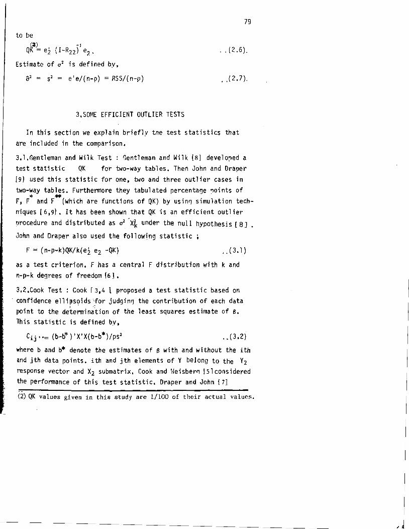
79

to be (2) -I

QK:::: ez (I-R22 ) ez. .. (2.6).

Estimate of cr2 is defined by,

&2 :::: S2 :::: e'e/(n-p) :::: RSS/(n-p) . ,(2.7).

3.S0ME EFFICIENT OUTLIER TESTS

In this section we explain briefly the test statistics that are inclUded in the comparison.

3.1 ,Gentleman and Wilk Test: Gentleman and Wilk [8] develored a test statistic QK for two-way tables. Then John and Draper [9] used this statistic for one, two and three outlier cases in two-way tables. Furthermore they tabul ated percentane ~oi nts of F, F * and F** (which are functions of QK) by usin~ simulation tech­niques [6,9], It has been shown that QK is an efficient outl ier procedure and distributed as cr2-X~ under the null hypothesis [8] .

John and Draper also used the following statistic i

F = (n-p-k)QK/k(e2 e2 -QK) ,.(3,1)

as a test criterion. F has a central F distribution with k and n-p-k degrees of freedom [61 •

3.2.Cook Test: Cook r 3,4 1 proposed a test statistic based on . confidence elli~soids~for judgin~ the contribution of each data

j' .-,­

point to the determination of the least squares estimate of B, This statistic is defined by,

Cij' '= (b-b") 'X'X(b-b*)/ps2 •• (3.2)

where band b* denote the estimates of 8 with and without the ith and jth data points. ith and jth elements of Y belong to the Y2 response vector and X2 sUbmatrix. Cook and Weisber~ [51 considered the performance of this test statistic. Draper and John [7]

(2) QK values given in this study are 1/100 of their actual values.

80

expressed Cij" as,

Cij •• = c ' Rzz C/pS2 .. (3.3),

and because of the equality

Cij" = ~2 [c;K- ] 3.3.Andrews and Pregibon Test

c'R22 c = c'c-QK, Cij"

: The Andrews and Pre~ibon

is

.. (3.4).

statistic AP is based on matrix of X* = (X:Y), the matrix of explanator:' variables appended with Y vector. This matrix for model in equa­tion (2.1) is,

Xl* = (X:Y) .(3.5),

and for mQdel in equation (~.3) is

X2 * = (X:D:Y) .. (3.1;)

where 0 = [~]. The Andrews-Pre~ibon statistic AP is defined as

* * * * R1j" = IXZ'X21II Xl'X l' .. (3.7),

ij •• denote the k subscrints selected to form Y2 [1]. Test statis­tic is based on the ryroportion of volume in xt attributable to the k observations which are nossible outliers. Dra~er and John [7]

established that. k

Rij"= (l-QK/RSS) II-R 221 = APlxAP2 =AP .. (3.8).

where AP1= (l-QK/RSS) and AP2= I I-R22, al so pronosed as two new outlier tests. Then Tatlldil [12] showed that APl has a beta dis­tribution with (n-9-k)/2 and k/2 degrees of freedom under the as­sumption that APl and AP2 are inde~endent. Tatlldil also showed that APl and AP (which has a central beta distribution with (n-r-l)/2 and p/2 de~rees of freedom) tests can be used for test­inq outliers in multivariate data. The critical values of AP and APl have been obtained by usin~ first and second order Bonferroni inequalities and these values have been tabulated for k=1(1)5 p=2(1)9 i n=5(1) 30(5)5()(1'»120 and a= n.01,O.05,f).10 [12].

i

81

4. SIllULATION STUDY

In this section. the ryercenta1e points of the test statistics QK. AP1. AP2. AP and Cij are obtained for each combination of o(num­ber of parameters) and n(samr>le size) while k(number of outlier)=l. The percentiles are estimated from the equations (2.6). (3.4) and (3.8) by using t10nte Carlo techn iques , 500 samo les Ilre generated for each case. Then the ~owers of the precedures are obtained for the same values of the narameters.

In the simulation study. a multirle renression model as

y. = X· B+ ••••+ X1.' Bp + ~.1. 1.1. 1. . P ~ i=1.2 •••• n .. (4.1)

is considered and it has two main stages.

In the first stage of the simulation the following steps are employed. i) n values of first column of X matrix are filled with 1 while other nx(p-l) values of the p-l columns wi~~ the valup.5 0 and 1. ii) n values of the residual vector £ are qenerated from N(O.l). oopulation. iii) n values of the response vector Yare obtained from the equa­tion in (4.1) iv) Test statistics QK. Cij • AP1. AP2 and AP are calculated from equations (2.6). (3.4) and (3.8). After repeating the process 500 times. the values of each test sta­tistic are sorted in ascendinn order. Then the upper percenta~e

points of QK and Cij and lower percenta~e points of AP1. AP2 and AP are recorded as critical values of these tests statistics. They are tabulated and given in A~ryendix A. Table A.l for p=2(l)5; n=10(5)40 and a=O.Ol.0.05 and 0.10.

The second stage of the simulation consist of two substanes. In the first sUbsta~e all the above stens are emnloyed except a dif­ference in the second step. That is a !lerturbation in the nth

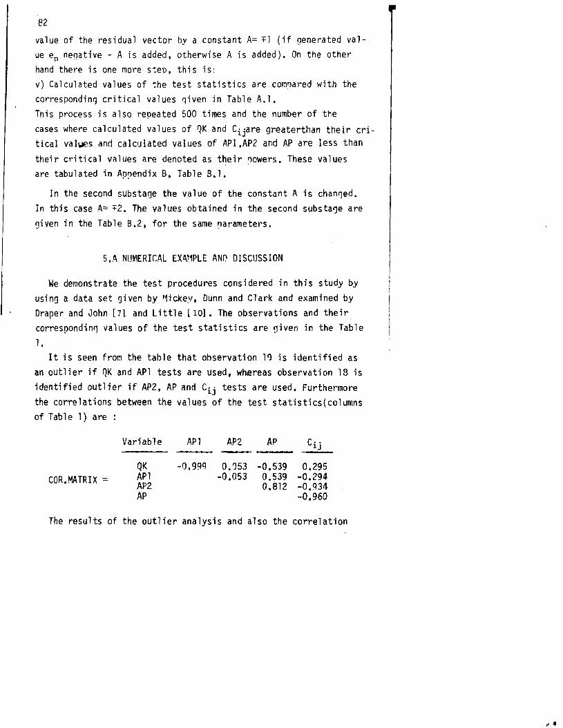
82

value of the residual vector by a constant A= +1 (if generated val­ue en negative - A is added, otherwise A is added). On the other hand there is one more step, this is: v) Calculated values of the test statistics are co~ryared with the corresponding critical values qiven in Table A.l. This process is also repeated 500 times and the number of the

cases where calculated values of QK and Cijare greaterthan their cri ­tical values and calculated values of APl,AP2 and AP are less than

their critical values are denoted as their ~owers. These values are tabulated in Ap~endix B. Table B.l.

In the second sUbsta~e the value of the constant A is chan~ed.

In this case A= +2. The values obtained in the second substa~e are ~iYen in the Table B.2, for the same narameters.

5•.n. NIJ\1ERlf.AL EXn.rWLE ANI') DISCUSSION

We demonstrate the test procedures considered in this study by usin~ a data set given by '1icke.v. Dunn and Clark and examined by Draper and John [71 and Little [101. The observations and their correspondin0 values of the test statistics are ~iven in the Table 1•

It is seen from the tahle that ohservation lq is identified as an outlier if QK and APl tests are used. whereas observ.ation 18 is identified outlier if AP2, AP and Cij tests are used. Furthermore the correlations between the values of the test statistics{columns of Table 1) are:

Variable APl AP2 AP C· .1J

QK -0.999 0.053 -0.539 0.295 APl -0.053 0.539 ~0.294COR.MATRIX = AP2 0.812 -0.Cl3tl AP -0.960

The resul ts of the outlier analysis and also the correlation

B3

TABLE 1.A~e at First Word(X), Gessel Adantive Score(Y) and their

correspond og Test Statistics Values.­

Case X Y '1K APl AP2 AP C.. ~J

1 15 95 0.043 0.998 0.952 0.950 0.009 2 26 71 1.084 0.953 0.845 0.806 0.081 3 10 83 2.598 0.887 0.937 0.832 0.072 4 9 91 0.820 0.964 0.929 0.896 0.026 5 15 102 0.857 0.963 0.952 0.917 0.017 6 20 87 0.001 1.000 0.927 0.927 0.000 7 18 93 0.124 0.995 0.942 0.937 0.003 8 11 100 0.067 0.997 0.943 0.941 0.002 9 8 104 0.107 0.995 0.920 0.916 0.')04

10 20 94 0.479 0.979 0.927 0.908 0.015 11 7 113 1.334 0.942 0.909 0.857 0.055 12 9 96 0.150 0.994 0.929 0.923 0.005 13 10 83 2.598 0.887 0.937 0.832 0.072 14 11 84 1.925 0.917 0.943 0.865 0.048 15 11 102 0.217 0.991 0.943 0.934 0.005 16 10 100 0.021 0.999 0.937 0.936 0.000 17 12 105 0.789 0.966 0.948 0.915 0.018 18 42 57 0.881 0.962 0.348* 0.335* 0.678* 19 17 121 9.686*0.580* 0.947 0.550 0.223 20 11 86 1. 396 0.939 0.943. 0.886 0.035 21 10 100_0..021 0.2,37 0.936 0.000, . 0.9.~9 .I • 'If ..

Unusual values High Low Low Low High are ~

matrix showed that QK and APl statistics tends to ~rovide similar results for outliers. In the discussions of the various authors such as Little [101. observation 19 was also identified as an out­lier. AP2, AP and Ci j statistics a~~roximatelv ~rovide the similar

results which was also mentioned in the ~revious works. These sta­tistics are sensitive to influential observations which have much affect on the fitted e~uation. As a conclusion ~K is the most

nowerful test amonq them.

Acknowledqements : The author would like to thank Prof.Or. Aydln tlztijrk and Associate Prof'.Dr. Soner ~~nen for their helnfu l com­ments and criticism.

.. <ii

ex> ~APPENDIX A CPITICAL VALUES OF TEST ~TATI~TJCS

TABLE A.1. Critical Values of QK. API. A~2. An and Cii ~tatistics Obtained fram S~0 ~enerations

for Various Values of nand p. .

P: 2 3 4 5

\est n n: 0.01 0.05 0.10 0.01 0.05 0.10 0,01 0.05 0.10 0.01 0.05 0.10

10 3.424 1.981 1.60~ 3.R24 2.172 1.67R 4.6h~ ~.700 2.25Q 1.024 2.527 1.902 15 3.783 1.986 1.542 3.217 2.961 1.542 1.616 2.685 1.845 1.192 2.710 2.027 20 3.881 1.805 1.365 2.447 2.098 1.456 1.892 2.078 1.701 4.001 2.6~9 ~.101

OK 25 3.588 2.678 1.648 4.599 2.486 1.Q84 4.165 3.208 2.131 1,961 2,466 1,772 . 30 2,440 2.148 1.803 3.851 1,874 1.60n 4.140 ?,73? 1.5~4 2,~87 1.868 1.436

35 3.617 2.328 1.840 3.345 2.553 2.052 3.096 2.562 1.640 1.511 2,01~ 1.597 40 1.504 1.872 1.648 2.979 1.678 1,407 1,318 2.855 1.851 4.476 2.501 1.754

10 0.389 0.589 0.649 0,437 0.563 0,660 0,197 0,412 0,475 0.301 0.410 0.466 15 0.604 0,750 0.837 0,508 0.729 0.770 0.h44 0.701 0,774 0.414 n.5~4 0,687 20 0,692 0.847 0.8Q6 0.724 0,801 0.852 0.662 0.785 0.829 0,660 0.725 O,R25

APi 25 0.693 0.840 0.894 0.757 0,828 0.860 0,677 0.769 0.791 0.657 0.8~4 n,87~

30 0.819 0,868 0.889 0,770 0.817 0.836 n,727 ~,826 0.~~2 0,78° 0.8Q5 n.Q0R 35' 0.843 0.881 0,921 ~.8h7 0.909 0.012 n.850 0.873 0,015 ~.77~ 0.81J 0,904 40 0,900 0,917 0.938 0.859 0.905 0,91° 0.846 0.884 0.~12 0.R13 0.8~1 n,q~8

10 0,421 0.543 0,579 0.387 0,428 0.513 0,282 0,141 0.102 0,137 0,lR7 0,277 15 0.545 0.612 0..718 0,445 0,469 n.5H 0.:152 0.45ft 'l.4Cl-R 0.171) 'l,{~04 n.S21 20 0,685 0,741 0.768 0,565 0,640 ~,682 0,501 0,59:1 0.~25 0.528 0.581 ~,~14

AP2 25 0.702 0.817 0,819 0.623 n.71S 0.777 0,571 0,657 0.692 0.623 0,680 0.732 30 0,771 0.829 0.881 0.620 0,711 0,769 0.644 0,725 0,760 0.670 0.725 0.753 3S 0.770 O,82Q 0.862 0.681 0,764 0,810 0.769 0,801 0.810 0.704 n.756 0.778 40 0.839 0.875 a.88q ,0.677 0,743 0,796 0,805 0.818 0,831 0.776 0.800 O.Rno

,

•

P. i¥.. ;; $ ij,. 4 .. >. ''')if, .><; .;0 "-.-'q.---­

TABLE A,l.(Continued)

P: 2 3 4 5

Test n a:0~010~0~ 0,10 0,01 n,05 n,10 O,n1 ~.n5 O,ln O,n1 n,05 n~ln

10 0,247 0,416 0,456 0,264 0,370 0.413 0,108 0,174 0,226 ",074 n.146 n,lhCl 15 0,513 O,56LO,631 0,369 0,448 0,492 0,326 0,370 0,440 n,264 n.152 n,181 20 0,618 0,671 0,728 0,449 0,565 0,~18 0,434 ",521 ".552 n,45Q n,SO" n.541

AP 25 0,665 0.780 '0,809 0,511 0,623 0,718 n,478 0,548 0,646 n,452 0,605 0,663 30 0,746 0,808 0,819 0,619 0,647 n,711 O,~06 O,6~5 0.705 0,616 0.669 0,706 35 0,743 O,79tl~~~~3 0,625 0,727 n,81~ ",711 n,7~4 n,77~ n,617 O,~85 0,728 40 0,803 0,852 0,8610,629 0,743 0,796 0,756 0,779 0.790 0.658 n,744 n,767

10 ~,413 0,688 0,487 1,154 0,471 0,308 '1,463 1,017 0,790 2,9n6n,900 n.666 15 0,501 0,258 0,148 0.916 0,374 0,298 0,747 n,471 0,349 n,870 0,518 ",183 20 0,404 0,226 0.161 0,884 0,288 0,116 0,551 O,3~1 n.2"5 0,407 0,362 0,216

c· .l.J 25 30

0,165 0,104 O,n76 0,160 0,128 0,089

0,430 0,282 0,135 0,274 0,147 0,092

0,553 0,408 0,237 0,300 n,l~4 n,l18

0.426 0,206 0,121 0,298 ".150 0,105

35" "O,288,O,170,/),110,0.155J).1180..096, 0,170 0.125 0.n810,2960.181 n,096 ~o 0,160 0,n93 0,"80 0,116 0,064 0,048 0,157 n,129 0,091 0,109 n,143 n.ln1

(X) (J1

... "II>,

APPENDIX B : POWERS OF TESTS OBTAINED F~O~ MnNTE-CA~L0 SIMULATIONS

co O"l

TABLE B.l. ?owers of the Tests and a while A= 1.

~K, API, AP2, AP and Cij for various Values of n, p

a: o.r» 1),05 n.ll) P n Test: QK API AP2 AP CLj nK AnI AP2 An CLi n~ API AP 2 An eii

In O,2n n.ln 0.n2 n.n5 O,n4 n.4b n.35 n.06 n.26 n.lS n,5Q n.47 n.ll n,12 n.2n 15 n.21 0,18 n,OO 0.18 n.16 n,55 n.43 n,n2 n,44 n.42 n,65 n,68 n.11 n,40 n.55 2n f),ln n,05 O,n2 n.lO 0.n7 n,56 f),54 n.ns n,ln n.2l I),~Q n,7l n.ll 1),1~ 1),29

2 25 3n

0,24 n,06 n,nl n,13 0.30 0,51 0.29 0.02 0.21 n,23

0.45 n.44 n.ln n,45 n,42 1).58 n.30 f).ln 0.39 n.2Q

n.nS n,n8 1),15 n.58 n,52 n.n7 n,5l n,17 n.42 n.37

35 4n

0,24 n,23 0,03 0.13 n,n9 0.18 n.34 0.03 0,16 n.lS

0.44 n.40 l).n4 n,21 n.22 n,S5 n,43 n.n7 n,37 n.3S

n,6l n.62 n.n8 n,37 1),18 n,n5 n,59 n.n9 0.46 n.4n

10 n,22 n,15 0.n4 n.12 0,03 0.42 n,32 n.os n.28 0,2n n.S5 n.45 0.16 n.35 n.35 15 n.20 n.07 n,02 0,03 n,n2 n.24 1).17 n,03 n,lO O.lQ n.n5 n.47 n.ns 1).26 n.14 20 0.3n 0.19 o.nl O,n7 n.02 0,51 0,36 o.n} 0,19 0,31 n.7l n.4Q f),nQ 0.3n n,48

3 25 0.19 0.27 0,02 0.02 n.OS n,5l n,4S n,n6 n,lS n.IS n.nS n,56 n,f)q n.45 n,47 30 0,27 0,07 0.01 0,05 n.lq 0.62 0,35 0,nl n.ll n,42 n,nS n,4Q n,12 n.ll n.57 35 0,37 0,43 0.00 n,Ol n,24 0,54 0.56 O,n2 n,21 0,29 ·0.62 n,76 0.09 n,54 0,37 40 n,30 O.2n 0,00 n,n2 n.2l O,n3 0.43 I),()n n,I)Q n.51 1),84 (J,6n n.n2 n.23 n.59

--._----­ .

......~ ...... I(14"'=t' .,,"oJ? """"".""..•...." .... ,.,

TABLE B.1. (Continued)

".10 qK API AP2 AP Cij.

n.45 n.11 n.ln n.2n fl.18 n.58 fl.59 fl.fl5 fl.26 fl.21 n,61 n,6? fl.l1 fl,24 0.44 n.sn n.24·0,14 fl,32 fl,25 fl.72 fl.64 fl,fl9 fl.31 n.44 fl,64 0.54 n.22 0.37 n,43 0,65 n.57 fl,12 n.37 n.38

fl,16 ",26 0.18 fl,2fl fl.18 0.40 n.41 n.1 0 n.29 0,28 n,48 n.S7 0.2fl n,32 O,2Q n.s7 0,58 0.26 1).36 n,41 fl,68 n,64 n.2no.43 0.44 0.61 0,52 n.21 n.44 0,51 n,64 n.54 n.18 n.3l fl,26

" a:

n Test:

4

In 15 21) 25 30 35 liB

5

10 15 21) 25 30 35 40

t·.

o.oi 1'1, os OK API AP2 AP C; j OK API AP2 AP Ci j

0.11 O,fl5 0,01 ",n5 fl.06 n,16 0.25 0.fl6 n,lo fl.14 0,23 0.3rrfl~no 0,09 0.060.4n O.4fl n.fl2 n.1S fl.ln 0.20 1).09 ~.01 0.n8 0.10 n.53 n.44 fl.fl5 0.22 n.17 0.20 0.11 I).no 0.n6 0.1)7 0.25 0.22 1'1.09 ",14 n,ll 0.20 0.07 .O~Ol 1),12 0,13 n.41 0.31 n.1)6 0.18 f'l.28 O.3n 1).24 0:03 n.13 0.22 0.35 1'1.31 n.ll n.34 0.26 0.32 0.22 0.08 0.24 0.17 n.40 n.44 O.I)~ n.11 n.26

0.19 O,n7 0.n1 0.04 0.010~290.1S n.05 n.13 n.1S 0.14 0,04 0.03 n.ns 0,06 0.36 0.17 0.17 n.23 O,lQ n.16 0.17 0.07 0.17 0.12 0.35 n.28 0.13 0.26 n,18 0.12 0,05 0,06 0.11 n.ll) n.41 ",37 n.17 0,22 0.20 0,34 0.23 0.06 0.22 0.11 0,56 n,54 n,ll fl,31 0.32 0.31.0.16.0,1)6 0.160.12 0.50 ..0,28 O,lS ..fl.2s ..n.21 0,14 O,O~ O,OS 0.07 0.n4 fl.45 0,38 0,13 0.25 fl.lS

en -...J

...

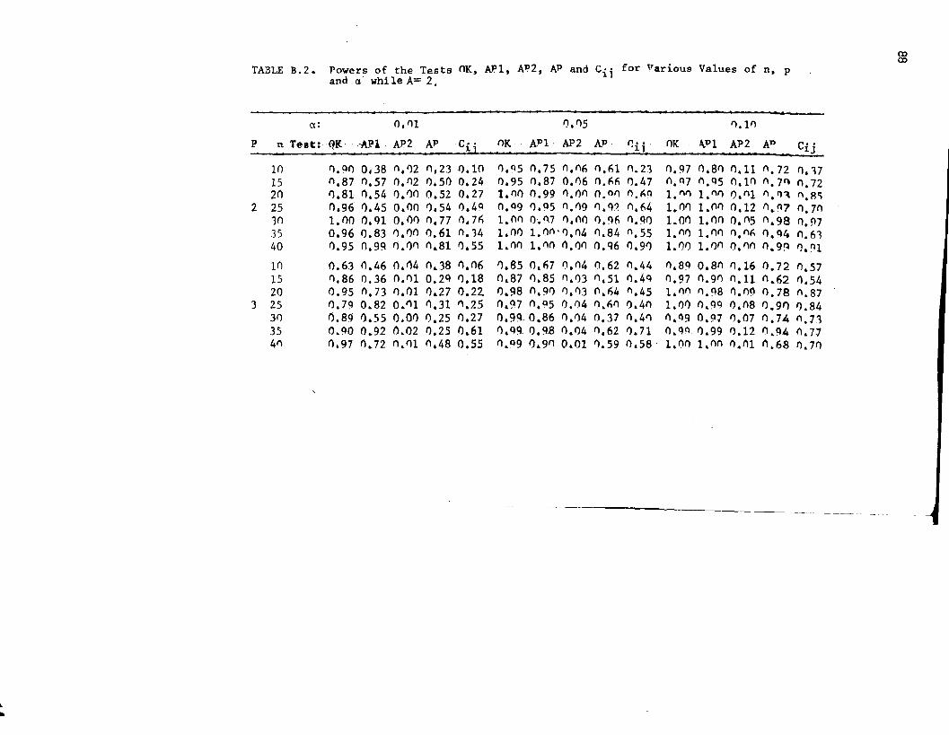
co

TABLE B.2. Powers of the Tests OK, A))l, ATJ2, A'P and Cii for Var Loue Values of n , p CD

and a' while A= 2.

P

2

3

(1: 0,1)1

nTelt:QK -,API· AP2 A'P C~.j

10 15 20 25 10 35 40

In 15 20 25 30 35 4n

1).~0 0,38 n,02 1).230.10 n,87 0,57 0,1)2 0,50 0,24 0,81 0,54 0.00 0.52 0,27 0,96 0.45 0.00 0,54 0.40

1.00 0,91 c.oo 0.77 n.7(, 0.96 0,83 1),00 0.61 n.14 0,95 0.99 0,on 0,81 0,55

0.63 0,46 0.04 n,38 1),06 n,86 0.36 0./)1 0.29 1).18 0,95 n,73 /).01 0.27 0.22 0.79 0,82 0,'11 1).31 '1.7.5 0,89 1.55 0.00 0.25 n.27 0.9-0 0.92 0.02 0.25 0,61 0.97 0.72 n,I)l 0,48 0.55

•

0,1)5

f)K - ATJl - A1'2 A'P - ~i i.

0,q5 0,75 1),1)6 1),61 1).21 0.95 0.87 0.06 0.~6 0.47 1.1)0 0.99 ~,on 0.01) n.~~

0,99 0.95 l).n9 I).9~ 0.64 1.M 0.007 0,00 1).96 1).90 1.00 1.(1)'/).04 n.84 n.55 1,1)0 1.nn n.on 0.96 n,90

0,85 0.~7 0,n4 0.62 n.44 0.87 1).85 1),1)3 n,51 0.49 0,98 n.90 1).f)3 0,64 n,45 0.~7 n,05 0.04 0.61) 0.40 0.99 0.86 0,04 0,37 0,41) 1).99 0.9.8 0,04 1).62 0.71

'I. If)

OK , TJ1 AP2 AT) Cij

0,97 0,81) 0.11 1),72 0,17 O.Q7 n.95 o,ln I). 7~ 0,72 1."f) 1."'1 0,n1 n.o~ n.R~

1.(1) l,nn 0.12 n,Q7 n.70 1.01'1 10M 0.n5 0,98 0.!'!7 1. n/) 1./)n n.n~ 1).94 0.61 1.00 1.l)n 0.1)0 0.9~ I).Ql

0,89 0.80 n.16 0.72 n.57 1).97 0.91) 0,11 0.62 0,54 1.0n 1).98 n,n9 0.78 n.87 1.00 0.99 n,n8 1).9n 0.84 1).99 0.91 1).07 0,74 n,71 O,9Q 0.99 1).12 n.94 0.71

n,09 0,91) 0.01 /),59 0,58' l.flO 1.nn 0.01 0.68 0,70

TABLE B.2. (Continued)

ex: 1).'11 n.1)5 n.1'l P n Test: OK AP1 AP2 A.P Cij 11K AP1 AP 2 AP Cij, ()K A.P 1 AP2, AP Cij

In 15

0.58 0.11 1),1)1 1).'14 0.11) 1).65 0,66 O.()2 0,27 n.22

n.~7

0,86 n,41 1).'11 n,15 n,17 n.7~ '1.'15 1).4'1 '1.17

1).lln n,Q1

n.~7

1).8Q 'l.1)1 'l.11) 'l.28 'l.ln '1.59 n.52

2n 1).75 n.61 l).n2 1).32 n.1~ 1).95 1).81 'l.'15 1').55 n.48 n.98 1),91 n.1l 'l.67 O,~5

4 25 0,74 1).45 o.nl) 0.22 1).23 1),91 1).81 n.I)Q 1).45 1).27 n.Q7 1).86 n.14 n.71 'l.54 30 0.81 1).45 'l.l)n 0.23 1).28 l,nl) n.8~ n,nn 0,41) n.~~ L nn l,n'l 1).1)1 'l.51 n.~7

35 n.97 0.85 n.1)2 ~.44 1).2~ 1.f)1) n.9A 1).02 n.71 1).42 L nn 1.n'l 'l,'15 '1.71 'l.51 41) O,Q7 n,84 0.n1 'l.33 1).52 1.0n 'l.Q4 1').1)1 1).54 n.78 1. nn l.'ll) 0.05 n.81 0.81

11) 0.51 0.3n 0.03 O.Oq '1.1)2 1).~4 1).54 n.1)5 1).13 n,24 '1.71 1).61 '1,18 n.4n n.32 15 n.71 n.28 0.03 0.25 0.16 'l.81 1).~5 1).17 n.48 '1.12 n.87 '1.sn n,l~ 'l.52 n.42 21') 'l.41 0.51 n.09 1).48 1).4n 1).85 n.?n 1).17 0.5Q '1.44 n.Q2 n,88 'l.lQ 0.74 '1,69

5 25 0.79 ~.43 0.07 'l.25 0.27 1').~1 n.88 0.1')8 'l.66 '1.57 n.96 n.97 '1.17 1).84 o,8n 3n 35 41)

0.85 0.60 0.04 n.50 1).30 0.87n~56,0.08 0.45 0.25 O.70 o.611) ,'090 .28 n.16

I).Q5 I).Q2 n.12 n.~5 n.~~

.n.Q7,,1).31 n.12.,n.5Q n.4~

0. <18 n.~.4 n.14 o, 75 o. ~ 1

n.~,:,

n.Q9 1).1'l1'l

'1,96 n.1~ 1).82 n.81 1).9Q n.15 'l.71 0.74 '1,Q6'1,14 '1,86 n.78

ex> 10

"

90 OZET

Bu cal rsmada daha 1nce Gentleman - !~ilk. Cook ve Andrews ­Prenibon taraf indan reeresvon modellerindeki ayk i r t de~erlerin

(outliers) test edilmesi icin ~nerilen y~ntemler incelenmistfr. ~onte-Carlo benzesim yontemi kullanllarak bu testlere iliskin kri ­tik de~erler ~=2(1)5; n=10(5)40 ve a=O.Ol. 0.05.0.10 icin tablo­l astt r-t lmts t i r , daha sonra ise yine aym parametre ler i cin y~ntem­lerin g~C de~erleri bulunarak karSllastlrllmlstlr. Son olarak da bu yontemlerin ~ecerlilikleri (elde edilen kritik de~erler kulla­m l arak) sayi sal bir ornek 'Izer inde incelenmistir.

RF.FF:ItENCES

1. Andrews. D.F. and Pre~ibon. D.~indin~ the outliers that matter. J.Roy. Sta.~oc•• Ser.B. 4n. 8s-Q3. 1978.

2. Beckman. R.J. and Cook. R.D. nutlier•••• s. Technometrics. 25. 2. 119-149. 1983.

3. Cook. R.D. Detection of influential .observation in linear re~ression. Technometrics. 19. 15-18. lQ77.

4. Cook. ~D. Influential observations in linear regression. JA~A. 74. 169-174. lQ79.

5. Cook. p.D. and Weisberg. S. Characterization of an emperical influence function for detectin? influential cases in regress­ion. Technometrics, 22. 4Qs-s08. lQ8n.

6. Draper. N.p. and John. J.A. Testin~ for three or fewer outliers in two-way tables. Technomet r i cs cvZz , 9-15. ll'l~O.

7. Draper. N.p. and John, J.A. lnfluential observations and out­liers in regression. Technometrics. 21. 21-26, 1981.

8. Gentleman. J.F. and Wilko M.B. Detectin~ outliers II: supple­mentin~ the direct analysis of residuals. Biometrics, 31. 387­410. 1975.

9. John. J.A. and Draper. N.R. nn testing for two outliers or one outlier in two-wav tables. Technometrics. 2n. fiQ- 78. lQ78.

lO.Little • .I .K. Influence and a quadratic form :tn the Andrews ­Pregibon statistics. Technometrics, 27. 11-1,. 1985.

ll.~osner. B. Percentage points for a generalized ESD manv out­lier procedure. Techn~etrics, 25, 2. 16,-172. lll83.

l2.Tatl~dil.~ Testing outliers in linear regression and multi ­variate data. Unpublished Doctoral Thesis, Hacettepe Univer­sity, Ankara, 1981.

.. I

acettepe Bulletin of lateral SCiences and Engineering 91

986/ Yol.-e 15/pp. 91-99

PARTIAL SOLUTION FOR STACKELBERG DISEQUILIBRIUM IN DUOPOLY

( 1) M S ( 1 ) ..E S " ozer • . ucu

In this study. we obtained a partial solution for the Stackelberg disequilibrium situation in a duopolistic market. by assuming the sum of the profit functions of two firms as the objective function of the multicriterion decision making problem and using two-person zero-sum game approach.

In order to get better understanding of the solution an application is given in Section 4.

Key words: Stackelberg disequilibrium. Duopoly

I. INTRODUCllON

In a duopolistic industry there are two sellers.There rare no generally accepted behavior assumptions for duopo­lists as there are for perfect competitors and monopolists. Different assumptions produce different solutions for 'duopolistic market. The well known solutions are cour not ,

collusion. Stackelberg. market shares and kinked demand curve,

In the Stackelberg solution one duopolist is leader ,while the other is follower. Duopolist. I is leader in the sence that he knows II I S reaction function. Each duopo­list determines his 'max.imum profit levels from both leader­

:ship and followership and desires to play the role which

(1) H~ccttcpe University. Ficulty of Science. Department of Statistics,

Ankara. TURKEY.

,. '.

·92

yields the larger profit. Four outcomes are possible: i) I desires t be leader and II a follower, ii) II desires to be a leader and I a follower, iii) both desire to be followers or, iv) both desire to- be leaders. The first two outcomes result in a determinate equilibrium which is known as Stackelberg solution. The third outcome results in Cournot's solution as shown in Henderson and Quandt [2,pp.230]. The fourth outcome is known as Stackelberg disequilibrium.

In this st4dy a solution for the Stackelberg disequilibrium case l ,. ,1

is obtained. In the duopolistic market when each of the duopolist desires to be leader, each duopolist thinks that he knows the other' reaction pattern and determines the profit-maximizing supply based a the other's reaction function but neither of the reaction functions is observed and Stackelberg disequilibrium comes into existence. Und this condition, over-production and different prices result in the market. After they become conscious of this situation they may reach an agreement in determining the price and the profit shares to maximize profits of each .other. This leads the market to a new part solution for the Stackelberg disequilibrium case. It is a partial, 'solution and not a definite solution because it comes about only if agreement between duopolists is reached.

2. METHOD

A game with two players where a gain to one player equals a loss to the other is known as a two-person zero-sum game [3,pp.339]. Each

. player has a finite number of strategies. The matrix which summarize the outcomes in terms of the gain (or loss) to one player, for all possible strategies of both 1l1ayers.-is -cal led the pay-off matrix.

The entries of the pay-off matrix lT kt (k= 1, .. 'I'P, t= 1, ... .p)

represent the expected gain for player I when he uses strategy k and player II uses strategy t. Let Ak be the probability that. player I will use strategy k, and ~t be the probability that player II will use strategy t. then

P A =1 ..(2. 1) l: k k=l

l:P JI. t=1 J.I t ~ 0 for all t .(2.2).

t=l

The expected pay-off for the game is given by,

p p p =~ l: IT kt Ak J.I t .,(2.3),k;;;'l t=l

Let Po be the minimum value of P and pO be the maximum value of P. T~e solution of the game con be obtained by solving either of the

following pairs of linear progranvning problems r 1,1973]:

1 ~ Min (-PQ ) =k~l .. (2.4)r k

s.t. ~ lT kt rk~l, ..(2.5) k=l

or

..(2.6)Max ( 1 )T p -.

S.t. ~ St ~ 1 s ~O . .<2.7) 7l kt t t=l

At the optimality,

* p* = pO = P* . ,<2.8) o

94

and

. (2.9)

where P* is optimal solution.

3. MODEL

Two firms are assumed to proQuce a homogenous product. The inverse demand function states the price as a function of the aggregate quantity sold:

.. (3.1)

where p is price. ql and q2 are quantities of the duopolists outputs. The profit of each equals his total revenue less his cost. which depends upon his output alone.

. .(3.2)

,,(3.3)

~Ihere lr1 and 11'2 are profits. Rl and R2 revenues. C1 and C2 costs of the first and the. second firms.

By assuming the sum of the profit functions of the firnls as the objective function of the multicriterion decision making prob­lem and using two person zero-sum game approach we may reach a par­tial solution for the Stackelberg disequilibrium situation.

Solving for tne leadership functions of I ur~ 'II "individually

we can determine q:'s and 1I'.·s under Stackelberg assumptions: 1 1

Forming pay-off matrix with entries of profits of the firms under leadership function of each of the firms. then using two person

95

zero-sum game method. optimal weights X.'s are obtained. and the1

compromise objective function "is.

2 'Ir= ~ X . 'Ir1 (q . ) . ,(3.4)

i=l 1 1

where Xi's are the optimal weights that firm I will use strategy i.

Then

•

4. APPLICATION

We use the example in Henderson and Quandt in order to get

a clear explanation of the partial solution [2.pp 226-231 l .

p =100-0.5 (ql q2) ..(4.1 )

Cl =5 ql . .(4.2)

_ 2 C2 ­ 0.5 q2 ..(4.3)

and the profits of the duopolists are

.. (4.4)

..(4.5).

For maximizing conditions of I and II we set appropriate

partial derivatives equal to zero:

()'lrl

d-"~-= 95 -ql-0.5 q2 = 0 . .(4.6)ql

chr _ ~ 2 = 100-0.5 ql -2 q2- 0 •. (4.7) •

2

96

The corresponding reaction functions are. q(= 95 -0.5 q2 .. (4.8) q2== 50 -0.25 ql .. (4.9).

The max imum leadership profit of I is obtained by substituting II's reaction function (4.9) into lIs profit equation(4.4).

..(4.10)

and maximizing with respect to ql we obtain

ql== 93.33 ~l== 3266.66

Under the leadership of I. the II's production and profit are

and ~2 =711.11 •

That is

-Lq - (93.33. 26.66) .

Likewise for the II's leaderahip and lIs followership assumptions the profit function of II is

. .<4.11)

and the solutions for maximizing are

q = 35 ~2=9l8.752

ql == 775 1T 1 = 3003. 125

that is

Each duopolist receives a greater profit from leadership. and both desire to act as leaders. Under this situation the reaction functions will never be observed and Stackelberg disequilibrium

, .

97

The pay-off matrix with entries 'II'.. is fanned aslJ

* Iq *t': q

'1'1 3266.66 3003.125

'11'2 . 711.11 918.75

Solving for optimal profit shares as in the case of two-

person zero-sum game technique, we get

3003.125 Al~ 918.75 A2 ;> p

where P is the value of the game, and

A*1 = . 440678

A* = .5593222

Maximize '1'= A1 7/'1 + A2 '1'2

=A1(95 ql ~0.5 q/) - 0.5 ql q2

. 2 .+A~ (l00 q2 -q2 ~0.5 ql q2 ) •

For maximization

The solutions are

ql =77 .64.705911

~2= 15.29411744

In that case we obtain the profits as

11'1 = 3768.17

11'2 =701.73

11' = 4469.2.

Also different solutions of the duopolistic market under different assumptions are summarized in lable 1 for comparison.

Table 1. Eguilibrium Values of the Price. Quantity Produced and Profit of the Duopolistic ~~rket

ell I h.~I,", C....r .... t St~ckr 1WI',! SoI"t I"n" H.... _Sulullun SOI.. tl .... I C~U. " " ". SOl.. l Ion._----­

""r~."l rrl<e ~1.a5 45 40 41.75 S).~~

Ikrket 'IS \10 IZO lIZ.5 90:.'" >,.., rt,.. I 90 80 93.33 11.5 n.ss~'I'- ... FI ... II 5 30 iIi.66 . 3S 15.29•• =' .:".. "-, ~"'...

Ivrkl:t 4525 "100 3~1J.18 3921.1175 ""fi9.!!.. Ora I 411S 3;,nn 3266.66 .3003.125 31LO.2...

0 F1 .. II 2!oO 900 m.lI!> 918.75 701.1~ ... -_._---­

a) The entries are taken from Henderson and Quandt 2. pp 175-186. b) This entry is different from the book.

99

aZET

Bu ~all~mada, iki satlclll piyasada, iki firmanln kar fonk­siyonlarl toplaml, ~ok ama~ll karar fonksiyonu varsayllarak, iki ­ki~ili slflr toplamll oyun yakla~lml ile Stakelberg dengesizligi durumunda klsmi ~ozOm elde edilmi~tir.

~ozOmOn daha iyi anla~llabilmesi i~in bir uygulama da ya­pi lm st i r ,

REFERENCES

1. Belenson, M. and Kapur, K.C. An algorithm for solving multi ­criterion Lt near- or-ogr-amminz with examples, Operat.ion Research Quarterly, 24 (1), 1973.

;:. Henderson, J.M. and Quandt, R. E. Microeconomic theory a mathe­matical approach, Mc Graw-Hill. Inc. 226-231, 1971.

3. Taha, H.A. Operation research an introduction, Second Ed. MacMillan Publishing Co. Inc. New York, 239-243. 1976.

.. 1

101 Hacettepe Bulletin of Natural Sciences and £ngineeriRg

1986/ Volu.e 15/pp. 101-108

A DYNAMIC REGRESSION ANALYSIS OF THE ENERGY CONSUMPTION BASED ON INCOME

C. Erdemir (1) S. Cakmak (1)

Based on annual data a dynamic regression model is built for the endo~enous time series Y = ener~y consumption and

. . t . 1exogenous ser~es x = per cap~ta gross nat~ona product. Dynamic regressiontmodels of which error terms fits to AR(n. AR(2), MA(n. ARMA(1. n . stationary stochastic processes are reviewed and maximum likelihood estimators of these models are introduced. It is concluded that the dynamic regression models are found more efficient than the classical regression model.

Key words: Dynamic Regression~ ARMA(p.q) Models. ML Estimators

INTRODUCTION

One of the assumptions of the classical linear regression model is the serlal independence of the disturbances, that is E(uu') =iI .

n A general linear model can be written in matrix notation in

the following manner:

Y = Xb + u

where. X is n x k matrix of the observations on exnlanatory variables and is assumed to be full rank, b is a k x 1 vector of parameters to be estimated, u is an n x 1 vector of stochastic disturbances. Fundamental assumptions of a normal classical linear regression model can be written out in the following

(l)Hacettepe Univ., Fac.of Sci., Statistics Dept., Ankara,TURKEY

102

manner: (1) Zero mean assumption: E(u) ~ O. (2) Homoscedasticity assumption + non-autocorre1ated error assumption: E(uu') = iI when In is an n by n identy-matrix. (3) Lackn, of simultaneity assumption: E(X'u) = O.

In practice, using ordinary least squares (QLS) estimates when disturbances of the model are autocorrelated is the possi­bility of non-sense relationships between time series when in reality there is no correlation between the series under investi ­gation. This point was first emphasized by Cochrane and Orcutt [3] and was later on formalized by Champernowne [2]. In order to avoid many complications and spurious results of the QLS regres­sion, some models are proposed; called dynamic regression models, where it is assumed that the ut error term follows a stationary stochastic process such as autoregressive process, AR(1), first order moving average process, MA(1), second order autoregressive process, AR(2) and the first order mixed autoregressive moving average process, ARMA(l,1): A brief review of the literature on the problem of dynamic regression can be found in Paseran and Slater [71.

DYNAMIC REhRESSION MODELS

Dynamic specifications of the models may occur in the stochastic parts as explained above. Besides that, the dynamic specifications of the regression model may occur in the deter­ministic part, named the distributed lag model. So, general linear regression equation can be written as:

k-2 00 , ,

Yt~ L b.xt· + bk 1 E AJ

xt_' k_1+bk. E AJ

Xt-J'.k+Uti =l' 1 - j =0 J , J =0 2 •

where ut is assumed to be specified by the process

ut - P1 - P2 ~ YVt - 1 + vt 'ut-1 ut-2 and vt is a pure random process. The notation P1 is used for

103

autoregressive parameters and Y is used for moving-averaqe process parameter. A is the parameter of the lao distribution and is assumed to be in the range 0 ~ A < 1.

The general model can be reduced to specific dynamic models under some assumptions on the parameters of >.., o , Y such as:

1) A1 = A2 = P1 = P2 = Y = 0, ordinary least squares, so that ut = vt. 2) A1 = A2 = P2 = Y = 0, first order autoregressive error specification with fixed initial value. AR(1), so that,

u - P1 ut _1 = v ' t t

3) >"1 = A2 = P2 =y= 0, first order autoregressive error *specification with stochastic initial values, AR (1), so that,

Ut - P1 Ut-1 = vt' 4) x1 = >"2 = Y = O. second order autoregress i ve error specification with stochastic initial value, AR(2), so that

- - P2 "i-z =ut P1 ut-1 vt' .

5) >"1 = >"2 = P1 = P2 = 0, first order moving averaqe error specification, MA(1), so that

u = v + YV ­t t t 1

6) >"1 = A2 = P2 = 0, first order mixed autoregressive-movinq average error specification, ARMA(1 ,1), so that

ut - P1 ut-1 = YVt -1 + vt' more dynami c model s depending on these parameters can be written.

7) P1 = P2 = Y = 0, distributed lag model with non-autorecor­related disturbances, so that

A1 ~ 0 and >"2 ~ 0 and ut = vt' 8) P2 = Y = 0, distributed lag model with first order auto­regressive error specification. so that

>"1 ~ 0, A ~ 0 and u - P12 t ut_1 = vt' Paseran and Slater [7].

104

The estimation method is based on maximum likelihood (ML) criterion as well as most of the estimation procedures currently used for all dynamic models. The ML estimators of the models with autocorrelated errors are computed using some iterative techniques.

These techniques carry out the estimation of dynamic regression models with autocorrelated errors under three different error specifications: (1) The Cochrane-Orcutt iteration procedure to compute P1 for AR(1) error specification with fixed initial values. (2) the inverse interpolation to calculate the AR(1) with stochastic initial values. (2) the modified Newton-Raphson iterative technique to compute P1 and P2 for the AR(2) error specification with stochastic initial values [3, 4, 1 ] •

Box and Jenkins [11. gives the ML estimators of the parameters of the regression model with first order moving-average disturb­ances. The derivation of the likelihood function of the ARMA process has been pursued recently by Newbold [6].

AN APPLICATION

In this chapter. a dynamic regression model of the consumption of energy was built based on per capita gross national product in 1968 retail prices in Turkey. The annual observations

for the variables are shown in Table 1. Some apPlications on the same data was done by Kocberber [51. Although use has tried to be made of first and second differences due to the autocor­relation in the data. nonacceptable results were obtained. In this study some dynamic regression models are tried and ML parameter estimates for different error specifications are given. The empirical work has been performed with computer programs developed by Pesaran and Slater [7]. Programs have been modified and applied to the B6800 system.

ML estimates of the parameters for dynamic models with differ­ent error specifications are given in Table 2.

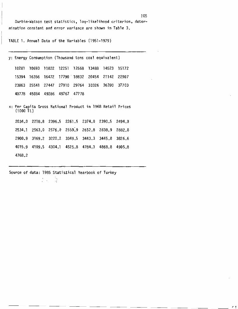
105 Durbin-Watson test statistics, log-likelihood criterion, deter­

mination constant and error variance are shown in Table 3.

TABLE 1. Annual Data of the Variables (1951-1979)

y: Energy Consumption (Thousand tons coal equivalent)

10281 10693 11822 12251 12568 13488 14523 15172

15394 16356 16472 17790 . 18832 20454 21142 22907

23863 25541 27447 27910 29764 33326 36390 37703

40778 45084 49286 49767 47778

x: Per Capita Gross National Product in 1968 Retail Prices (1000 TL)

2034.0 2218.8 2396.5 2261.5 2374.0 2390.5 2494.0

2534.1 2563.0 2576.0 2559~9 2652.8 2838.9 2882.8

2900.9 3169.2 3220.2 3349.5 3443.3 3445.8 3826.6

4015.9 4109.5 4304.1 4525.8 4784.3 4868.8 4905.8

4768.2

Source of data: 1985 Statistical Yearbook of Turkey

...

106

4

5

TABLE 2. Error Specifications and Related Models

Model Error Number Specification Model

AR( 1) Fixed Initial Values

2 *AR(1) Stochastic Initial Values

3 A(2) Stochastic Initial Values

Yt = -19924.8 + 13.75 xt u = 0.50 ut-1 x vt •t

Yt = -18629.4 + 13.43 xt = 0.55ut ut-1 x vt

Y = -13609.3 x 13.40 xtt u = 0.63 u ut t_ 1-O.l7 t_2+v t

MA(1) Y = -18958 x 13.50 xtt ut = 0.53 xt - 1 x vt

ARMA( 1.1) Yt = 18665 x 13.42 xt ut - 0.20 Ut_1=0.4lvt_1+Vt

6 Stochastically Yt = -19197.1 + 13.55 Xt Independent Error ut = v(SIE) t

107

TABLE 3. The Test Statistics of the Models

Model Error Durbin- Log­ R2 2 cr

No. Specification Watson Li keli hood Residual

1 AR( 1) 1.76 -195.03 0.99 1161 2 *AR( 1) 1.82 -202.84 0.99 1122 3 AR(2) 1.93 -202.49 0.99 11 09 4 MA(l) 1.70 .-202.84 0.99 1135 5 ARMA( 1.1) 1.86 -202.67 0.99 1124 6 SIE 0.90 -207.06 0.90 1307

The detennination constants, R2, obtained for each model area very high. There is no statistically significant difference between the constants. On the other hand, it is shown that the error variances are not different from each other except in the sixth model. Hence, the 10g-likQlihood function value is an ac­ceptable criterion for selecting the best model. Finally, the first model was accepted as a useable model which has a maximum log-likelihood value.

CONCLUSION

As a result, a dynamic moder which can be used for prediction and description is propose~ at the end of the modelling process.

It has been shown that dynamic regression models must be prefered when data arises as a time series and autocorrelations cannot be removed from residuals.

108

tYZET

Dlssal degisken Yt=Yllllk enerji tUketimini icsel degisken xt=kiSi baSlna ulusal gelir olan t yllllk veriye dayall bir dinamik regresyon mode1i kuru1mustur. Hata terimini AR(l)t AR(2), MA(l), ARMA(l ,1) duragan stokastik sllrec lere uyduqu

dinamik regresyon mode11eri ince1enmis ve bun1arln en cok olabilirlik tahmin edicileri tanltllmlstlr. Sonucta, dinamik regresyon modellerinin klasik regresyon modellerine gore daha etkin oldugu gorU1mUstUr.

REFERENCES

1.Box, G.E.P. and Jenkins, G.M. Time series analysis forecasting and control, Holden Day, San Francisco, 1970.

2. Champernowne, D.G., An experimental investigation of the robust­ness of certain procedures for estimating means and regression coefficients, J. Roy. Stat. Soc. A 123, 39B-4l2, 1960.

3.Cochrane, D. and Orcutt, G.H., Application of least squares regression to relationships containing autocorrelated error terms, J. Am., Stat. Ass. t 44, 32-61, 1949.

4.Hartree, D.R. Numerical analysis (2nd ed.), Charendon Press, Oxford, 195B.

5.Ko~berber, E., Tlirkiye enerji tliketim"analizleri, DiE, 19B4.

6.Newbold, P., The exact likelihood function for a mixed auto­regressive-moving average process, Biometrica 61, 423-426, 1974.

7.Pesaran, M.H. and Slater, L.J. t Dynamic regression: Theory and algorithms. John Wiley, New York, 19BO.

. ..

APPENDIX

I

I

109 Hacettepe lulletin of latural Sciences and Engineering

1985-1986/ Vol... 1~-15/pp. I09-11Z

PREPERATION OF FINAL TYPESCRIPT* - APPLIED AND EXPERIMENTAL SCIENCES ­

E. Board( 1)

This article gives instructions for preparing the final typescript of your paper. It is laid out according to these rules, and may be used as a guide. Please indent the abstract three spaces from the left and right margins, as shown here.

Key words: Type styles, Layout, Spacing

INTRODUCTION

The rules below amplify the mrormat ton given in [1] , and aim at giving the bulletin a uniform and pleasing appearance. Please follow them carefully. The Editorial Board are under no ob l igation to publish typescripts not conforming to these rules. Please note that the page numbers and publication identifier (top of page one) will be added during publication, but you should number the pages well outside the printing area, so they may be kept in order.

~ATERIALS AND METHODS

The final typescript should be prepared on an electric typewriter employing a black plastic ribbon and one of the following typefaces

(a) For the main text: IBM letter Goth 96 or OLYMPIA 808

(1) Hacettepe University, Faculty of Science, Ankara, TURKEY.

* Replaces all previous instructions.

110

(b) For the abstract, references, footnotes, subscripts, and super­scripts:

IBM Prestige Elite 96 or OLYMPIA 802

12 Pitch (12 characters per inch) should be used throughout. The main title and subheadings should be in upper case. Bold face type may be used to highlight newly defined terms, important phrases, etc. Do not use underlining. Special symbols, foreign letters, etc., should be typed whenever possible.

The typing area is 14cmx22cm, giving 52 lines and 66 characters per line at 12 pitch. Only material within this area will appear in print.

The main title and subheadings should be centred. Displayed formulae, etc., may also be centred if desired.

There should be an indentation of three spaces at the beginning of each new paragraph. Part identifiers, such as (a), (b), etc., should also be indented three spaces from the left hand margin.

The (first line of the) ~ain title should be typed on line 8, the authors name(s) on line 14 and the first line of the abstract on line 17. Where there is more than one author the format for the names is A. Abe I ( 1), B. Cox ( .), ••• • Af.ter the fi rst page the text should begin on line 3. The following table gives the rules for line spacing.

TABLE 1. Line Spacing.

Spacing Application

1/2 { Subscripts, superscripts. 1 { Abstract. Two lines of the same reference or footnote

Norma I text. Between two references or footnotes. Double-lined title or heading. Bet ween text and heading to a table or figure.

2 { To emphasize a formula or block of text. 2 1/2 { Between a subheading and following text or item. 3 1/2 { Between text and following subheading.

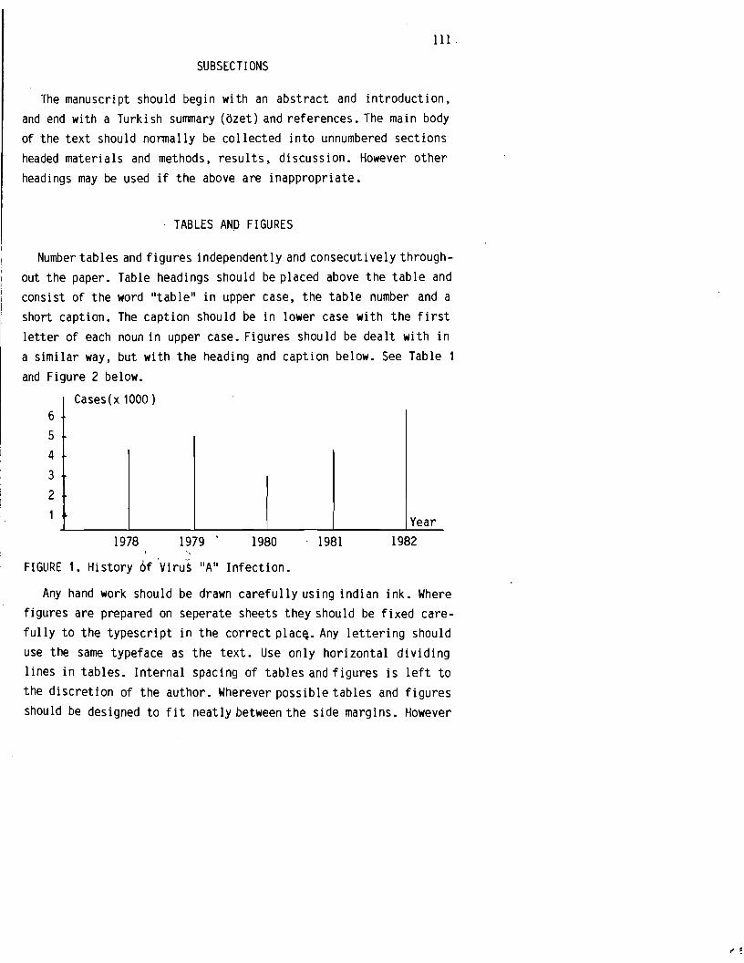
111

SUBSECTIONS

The manuscript should begin with an abstract and introduction, and end with a Turkish summary (ozet ) and references. The main body of the text should normally be collected into unnumbered sections headed materials and methods, results, discussion. However other headings may be used if the above are inappropriate.

TABLES ANp FIGURES

Number tables and figures independently and consecutively through­out the paper. Table headings should be placed above the table and consist of the word "table" in upper case, the table number and a short caption. The caption should be in lower case with the first letter of each noun in upper case. Figures should be dealt with in a similar way, but with the heading and caption below. See Table 1 and Figure 2 below.

Cases (x 1000 ) 6

5

4

3

2

1 Year 1978 1979 . 1980 , 1981 1982

FIGURE 1. History 6f 'Viru~ "A" Infection.

Any hand work should be drawn carefully using indian ink. Where figures are prepared on seperate sheets they should be fixed care­fully to the typescript in the correct plac~. Any lettering should use the same typeface as the text. Use only horizontal dividing lines in tables. Internal spacing of tables and figures is left to the discretion of the author. Wherever possible tables and figures should be designed to fit neatly between the side margins. However

112

very long tables or figures may, together with their headings, be set lengthwise along the page. A page may contain more than one figure or tab le set lengthwi se , but on no account should it contain any text.

MISCELLANEOUS NOTES

(a) footnotes. Footnotes to page one should give the address(es) of the author(s) and acknowledments for financial assistance. In other cases footnotes should be avoided.

(b) References. The punctuation of references is given inside the back cover of the bulletin, to which reference'should be made.

(c) Acknowledgments. Personal acknowledgments may be placed just before the Turkish Summary (~zet), as shown below.

Acknowledgment. The author would like to thank ...

~ZET

Bu makale, yezim zm son sekl inin nazir leru sr ile ilgili kural lar i ic;ermektedir. Aym zamanda kendisi bu kuraI-lara gore hez i r landrqr

ic;in bir ornek te~kil etmektedir.

REFERENCES

1. Board, E. Submission of manuscripts. Hacettepe Bulletin of Natural Sciences and Engineering, 14, Inside back cover, 1985.

Hacettepe Bulletin of Natural Sciences and Engineering II3 1985-1986/ Volule 14-15/pp. 11'-116

PREPERATION OF FINAL TYPESCRIPT* - MATHEMATICS AND THEORETICAL STATISTICS ­

E. Board ( 1)

This article gives instructions for preparing the final typescript of your paper. It is laid out according to these rules, and may be used as a guide. Please indent the abstract three spaces from the left and right margins, as shown here.

Key words: Type styles, Layout, Spacing

1980 Subject Classification: 00A20

1. INTRODUCTION

The rules below amplify the. information given in [1] , and aim at giVing the bulletin a uniform and pleasing appearance. Please follow them carefully. The Editorial Board are under no obligation to publish typescripts not conforming to these rules. Please note that the page numbers and publication identifier (top of page one) will be added during publication, but you should number the pages well outside the printing area, so they may be kept in order.

2. APPROVED TYPE STYLES

The final typescript should be prepared on an electric typewriter employing a black plastic ribbon and one of the following typefaces

(a) For the main text: IBM letter Goth 96 or OLYMPIA 808

(1) Hacettepe University, Faculty of science, Ankara, TURKEY.

* Replaces all previous instructions.

" i

114

(b) For the abstract, references, footnotes, subscripts and super­scri pts:

IBM Prestige Elite 96 or OLYMPIA 802

12 Pitch (12 characters per inch) should be used throughout. The main title, subheadings and numbered section headings should be in upper case. Bold face type may be used to highlight newly defined terms, important phrases, etc. Do not use underlining. Mathematical symbols, foreign letters, etc., should be typed whenever possible. Where script letters are called for, but not available, please use the nearest typeable alternative (eg. upper case italic or bold­face) •

3. LAYOUT AND SPACING

The typing area is 14cmx22cm, gIVIng 52 lines and 66 characters per l Ine at 12 pitch. Only material within this area will appear in print.

The main title and subheadings should be centred. Displayed formulae, etc., may also be centred if desired.

3.1. DEFINITION. Text which forms part of a numbered item (remark, definition, statement or proof of a theorem, etc.) will be called bound, all other text will be called free.

There should be an indentation of three spaces at the beginning of each new paragraph. Each new block of free text should begin with a paragraph indentation, but bound text should not contain para­graph indentations. However the word "proof II, and part identi f iers such as (a), (b), etc., should be indented three spaces. An example IS seen in the layout of Theorem 3.2 below •

3.2. THEOREM. let (x ) be a convergent sequence in the Hausdorff n

space X. Then: (a) Every subsequence of (x ) is convergent.

n (b) The limit of (x ) is unique.

n

115

Proof. (a.) Immediate from the definition. (b) Suppose x ~ yare lImlt s of (x ). Then if Mand N are

n arbitrary neighbourhoods of x, y respectively

The (first line of the) main title should be typed on line 8, the authors name(s) on line 14 and the first line of the abstract on li ne 17. Where there is more than one author the format for the names is A. Abel (1) , B. Cox (.), •... After the fi rst page the text should begin on line 3. The following table gives the rules for line spacing.

3.3. TABLE. Line Spacing.

Spacing Application

1/2 { Subscripts, superscripts. 1 { Abstract. Two lines of the same reference or footnote

Normal text. Between two references or footnotes. Double-lined title or heading. Bet ween statement-and proof of a theorem, etc.

2 { Between bound and free or bound and bound text. 2 1/2 { Between a subheading and following text or item. 3 1/2 { Between text and following subheading.

Where subscripts, superscripts, etc., are involved the above spacing may be increased the minimum necessary to maintain clarity.

3.4. EXAMPLE. Increased Spacing. •• x •••••• • •••• x •••

(a) a (b) a .•••••2n •• • ••• 2n

•••

Try to avoid case (b) by rearranging the text. Also avoid the use of subscripted subscripts, etc.

4. MISCELLANEOUS NOTES

(a) Tables, Diagrams, Graphs, etc. These should be treated as

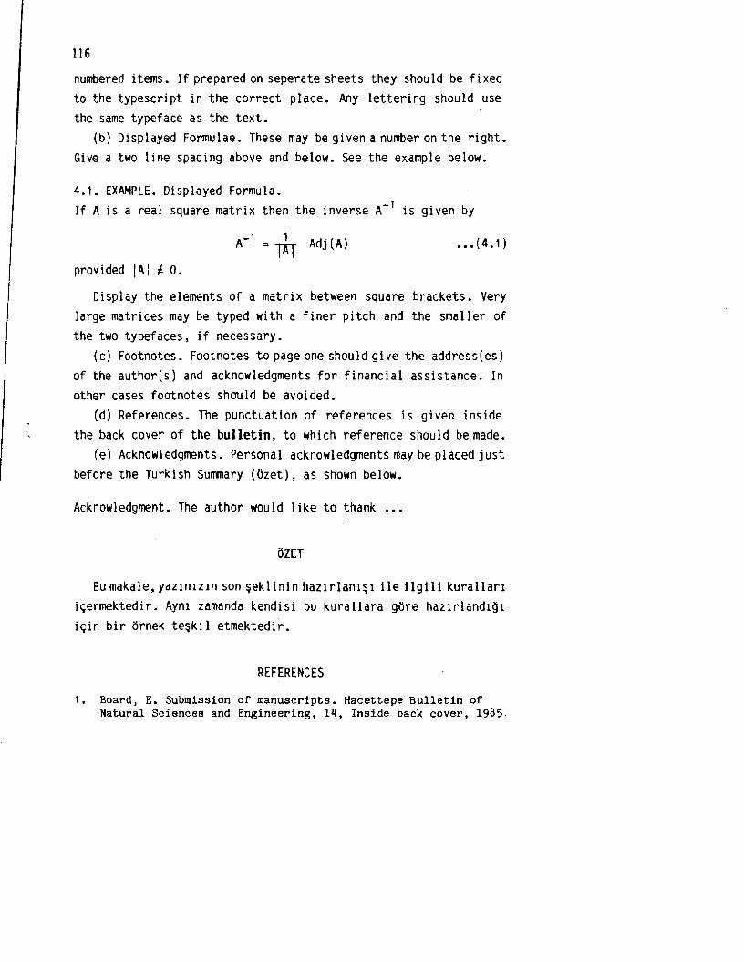
116

numbered items. If prepared on seperate sheets they shou ld be fi xed to the typescript in the correct place. Any lettering should use the same typeface as the text.

(b) DispIayed Formu Iae. These may be given a number on the ri ght. Give a two line spacing above and below. See the example below.

4.1. EXAMPLE. Displayed Formula. If A is a real square matrix then the inverse A- 1 is given by

A- 1 = ~ Adj(A) .•• (4.1)

provided IAI ~ o. Display the elements of a matrix between square brackets. Very

large matrices may be typed with a finer pitch and the smaller of the two typefaces, if necessary.

(c) Footnotes. Footnotes to page one should give the address(es) of the author(s) and acknOWledgments for financial assistance. In other cases footnotes should be avoided.

(d) References. The punctuation of references is given inside the back cover of the bulletin, to which reference should be made.

(e) Acknowledgments. Personal acknowledgments may be placed just before the Turkish Summary (Ozet). as shown below.

AcknOWledgment. The author would like to thank

DIET

Bu makale, yaziru zm son sekl inin haz i r larus i i Ie ilgi l i kureIl ar i i~ermektedir. Aynl zamanda kendisi bu kurallara gore hazlrlandl~i

i~in bir ornek te~kil etmektedir.

REFERENCES

1. Board, E. Submission of manuscripts. Hacettepe Bulletin of Natural Sciences and Engineering, l~, Inside back cover, 1985,